Remarks on the Bernstein inequality for higher order operators and related results

Abstract.

This note is devoted to several results about frequency localized functions and associated Bernstein inequalities for higher order operators. In particular, we construct some counterexamples for the frequency-localized Bernstein inequalities for higher order Laplacians. We show also that the heat semi-group associated to powers larger than one of the laplacian does not satisfy the strict maximum principle in general. Finally, in a suitable range we provide several positive results.

1. Introduction

This note is devoted to several results about frequency localized functions and associated Bernstein inequalities for higher order operators. We consider a class of fractional Laplacian operators acting on frequency localized functions on the whole space $\mathbb{R}^{d}$ or the periodic torus. To fix the notation, we use the following convention for Fourier transform on $\mathbb{R}^{d}$, $d\geq 1$:

$$f(x)=\frac{1}{(2\pi)^{d}}\int_{\mathbb{R}^{d}}\widehat{f}(\xi)e^{i\xi\cdot x}d\xi;$$ (1.1)

$$\widehat{f}(\xi)=\int_{\mathbb{R}^{d}}f(x)e^{-i\xi\cdot x}dx.$$ (1.2)

For $s>0$, we define the fractional Laplacian operator $\Lambda^{s}=(-\Delta)^{\frac{s}{2}}$ via the Fourier transform:

$$\widehat{\Lambda^{s}f}(\xi)=|\xi|^{s}\widehat{f}(\xi),\qquad\xi\in\mathbb{R}^{d}.$$ (1.3)

In yet other words $\Lambda^{s}$ corresponds to the Fourier multiplier $|\xi|^{s}$. Note that for $s=2$ we have $-\Lambda^{s}=\Delta$, i.e. the usual Laplacian operator. For $0<s\leq 2$, it is known (cf. [2], [7], [11] and the references therein) that the following frequency-localized Bernstein-type inequality hold: for $1<p<\infty$ and any band-limited $f\in L^{p}(\mathbb{R}^{d},\mathbb{R})$ with

$$\text{supp}(\widehat{f})\subset\{\xi:\;\gamma_{1}\leq|\xi|\leq\gamma_{2}\},$$ (1.4)

there are constants $A_{1}>0$, $A_{2}>0$ depending only on $(d,p,s,\gamma_{1},\gamma_{2})$ such that

$$A_{2}\|f\|_{p}^{p}\leq\int_{\mathbb{R}^{d}}(\Lambda^{s}f)|f|^{p-2}fdx\leq A_{1}\|f\|_{p}^{p}=A_{1}\int_{\mathbb{R}^{d}}|f|^{p}dx.$$ (1.5)

Note that for $p=2$, the above inequality is trivial thanks to the usual Plancherel theorem. The main point of (1.5) is that it continues to hold for $p\neq 2$ where the Fourier support of the associated functions have nontrivial overlapping interactions.

By a scaling argument, if $h\in\mathcal{S}(\mathbb{R}^{d})$ has frequency localized into $\{|\xi|\sim N\}$ where $N\gg 1$, then it follows from (1.5) that (below $0<s\leq 2$ and $1<p<\infty$)

$$\int_{\mathbb{R}^{d}}\Lambda^{s}h|h|^{p-2}hdx\geq\;\mathrm{const}\cdot N^{s}\|h\|_{p}^{p}.$$ (1.6)

Such powerful estimates have important applications in the regularity theory of fluid dynamics equations (cf. [11]). For example, consider the dissipative two-dimensional surface quasi-geostrophic equation

$$\partial_{t}\theta=-\Lambda^{s}\theta+\Lambda^{-1}\nabla^{\perp}\theta\cdot\nabla\theta,$$ (1.7)

where $0<s\leq 2$. Applying the Littlewood-Paley project $P_{j}$ which is localized to $\{|\xi|\sim 2^{j}\}$ and calculating the $L^{p}$ norm of $P_{j}\theta$, we obtain

$$\frac{1}{p}\partial_{t}(\|P_{j}\theta\|_{p}^{p}) =-\int_{\mathbb{R}^{d}}(\Lambda^{s}P_{j}\theta)|P_{j}\theta|^{p-2}P_{j}\theta dx+\text{Nonlinear terms}$$ (1.8)

$$\leq-\mathrm{const}\cdot 2^{js}\|P_{j}\theta\|_{p}^{p}+\text{Nonlinear terms},\qquad(\text{by Bernstein}).$$ (1.9)

From this and using additional (nontrivial) commutator estimates, one can deduce fine regularity results in various critical and subcritical Besov spaces (see recent [8] for an optimal Gevrey regularity result and the references therein for earlier results). On the other hand, it has been long speculated whether the above Bernstein inequalities also hold for higher order Laplacian operators $\Lambda^{s}$ for $s>2$. The purpose of this note is to demonstrate some counterexamples around these higher operators $\Lambda^{s}$. Our main results are the following.

• Biharmonic operator. See Theorem 2.1. We show via an explicit construction the failure of Bernstein inequalities for the biharmonic operator $\Delta^{2}$ with $p=4$.

• Lack of positivity for higher order $e^{-\Lambda^{s}}\delta_{0}$, $s>2$. See Theorem 3.1. We give two proofs to show the general lack of positivity for the higher order heat operators. Some sharp asymptotic decay at spatial infinity is also shown.

• Counterexamples for Bernstein for $s>2$, $p\in(1,p_{0})$ or $p\in(p_{1},\infty)$ for some $p_{0}<2<p_{1}$. See Theorem 3.2 and Theorem 3.3. For general operators $\Lambda^{s}$ with $s>2$, we show generic failure of Bernstein inequalities for $p=1+$ or $p=\infty-$.

• Some periodic Bernstein inequalities for $\Lambda^{s}$, $0<s\leq 2$. See Theorem 4.1 and Theorem 4.2. By using a nontrivial complex interpolation argument together with some concentration inequality, we prove a family of Bernstein inequalities for mean-zero periodic functions for all $p\in(1,\infty)$. We also show frequency-localized versions in Theorem 4.2.

• A Liouville theorem for $\Lambda^{s}$, $s>0$. See Theorem 5.1. We prove a rigidity type for the ancient solutions to a fractional heat equation.

The rest of this note is organized according to the above summary.

Notation

For any two positive quantities $X$ and $Y$, we write $X\lesssim Y$ or $X=O(Y)$ if $X\leq CY$ for some unimportant constant $C>0$. We write $X\ll Y$ if $X\leq cY$ for some sufficiently small constant $c>0$. The needed smallness is clear from the context. We write $f\in L^{p}(\Omega,Y)$ if $f:\;\Omega\to Y$ and is in $L^{p}$. For example $f\in L^{2}(\mathbb{R}^{3},\mathbb{R}^{2})$ means $f$ is $\mathbb{R}^{2}$-valued and

$$\|f\|_{2}^{2}=\int_{\mathbb{R}^{3}}|f|^{2}dx=\int_{\mathbb{R}^{3}}(f_{1}^{2}+f_{2}^{2})dx<\infty,\qquad\text{here $f=(f_{1},f_{2})^{\mathrm{T}}$}.$$ (1.10)

For a complex number $z=a+bi$ with $a,b\in\mathbb{R}$, we denote $\mathrm{Re}(z)=a$ and $\mathrm{Im}(z)=b$.

We denote the usual sign function $\mathrm{sgn}(x)=1$ for $x>0$, $-1$ for $x<0$ and $0$ if $x=0$.

We use the Japanese bracket notation $\langle x\rangle=\sqrt{1+|x|^{2}}$ for any $x\in\mathbb{R}^{d}$, $d\geq 1$.

2. Failure of Bernstein inequalities

Theorem 2.1.

Let the dimension $d\geq 1$. There exists a sequence of Schwartz functions $f_{j}:\;\mathbb{R}^{d}\to\mathbb{R}$ with frequency localized around $N_{j}\to\infty$, such that

$$-C_{2}<\frac{\int_{\mathbb{R}^{d}}\Delta^{2}f_{j}f_{j}^{3}dx}{N_{j}^{4}\int_{\mathbb{R}^{d}}f_{j}^{4}dx}<-C_{1}<0.$$

In the above $C_{1}>0$, $C_{2}>0$ are constants depending only on $d$. More precisely, the frequency support of $f_{j}$ satisfies

$$\mathrm{supp}(\widehat{f_{j}})\subset\{\xi:\,\alpha_{1}N_{j}<|\xi|<\alpha_{2}N_{j}\},$$

where $\alpha_{1}>0$, $\alpha_{2}>0$ are constants depending only on $d$.

Remark 2.1.

By a perturbative argument, one can also show counterexamples for $\Lambda^{s}$, $|s-4|\ll 1$.

Lemma 2.1.

Consider $f_{1}(x)=\log(1+x^{2})$, $x\in\mathbb{R}$. Denote $f_{1}^{(4)}(x)=\frac{d^{4}}{dx^{4}}(f_{1}(x))$. Then

$$I_{1}=\int_{\mathbb{R}}f_{1}^{(4)}(x)f_{1}(x)^{3}dx<0.$$

Remark 2.2.

One can take for example $f_{2}(x)=x+e^{-x^{2}}$ to obtain

$$\int f_{2}^{(4)}(x)(f_{2}(x))^{3}dx\approx-2.47784<0.$$ (2.11)

However the issue with $f_{2}$ is that it is not amenable to localization. Namely if we consider

$$\int(f_{2}(x)\phi(\frac{x}{R}))^{(4)}(f_{2}(x)\phi(\frac{x}{R}))^{3}$$ (2.12)

for a bump function $\phi$ and $R$ large, then the main order term is

$$\int(x\phi(\frac{x}{R}))^{(4)}(x\phi(\frac{x}{R}))^{3}dx=R\int(x\phi(x))^{(4)}(x\phi(x))^{3}dx$$ (2.13)

which may not take a favorable sign. This subtle issue disappears for the function $f_{1}(x)=\log(1+x^{2})$ due to its mild growth at spatial infinity.

Remark 2.3.

Interestingly, if we work with $\frac{d^{8}}{dx^{8}}$ instead of $\frac{d^{4}}{dx^{4}}$, then we have for $f_{2}(x)=x+e^{-x^{2}}$,

$$\int f_{2}^{(8)}(x)(f_{2}(x))^{3}dx\approx-219.804<0.$$ (2.14)

One may then take $f_{2,R}(x)=f_{2}(x)\phi(x/R)$ for $R$ sufficiently large to show

$$\int f_{2,R}^{(8)}(x)(f_{2,R}(x))^{3}dx<0.$$ (2.15)

This can be used to construct frequency localized counterexamples for $\Lambda^{8}=(-\partial_{xx})^{4}$.

Remark 2.4.

To obtain $I_{1}<0$, we can also adopt a more numerical approach in lieu of exact contour integral computation. To this end, denote

$$g(x)=f_{1}^{(4)}(x)f_{1}(x)^{3}=-12\frac{(1-6x^{2}+x^{4})(\log(1+x^{2}))^{3}}{(1+x^{2})^{4}}.$$ (2.16)

A schematic drawing of $g(x)$ for $x\in[0,0.5]$ and $x\in[0,10]$ can be found in the figures below.

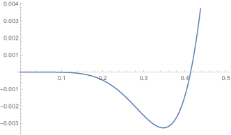
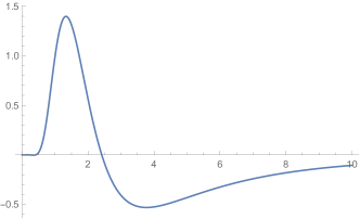
Figure 1. The plot of $g(x)$ for $0\leq x\leq 0.4$ and $0\leq x\leq 10$

By examining the polynomial $1-6x^{2}+x^{4}$ in the definition of $g(x)$, it is easy to check that $g(x)>0$ for $x\in(\sqrt{2}-1,\sqrt{2}+1)$ and $g(x)<0$ for $x<\sqrt{2}-1$ or $x>\sqrt{2}+1$. In particular

$$I_{1}<2\int_{0\leq x\leq 10}g(x)dx\approx-1.65835.$$ (2.17)

Proof.

To ease the notation we write $f_{1}$ as $f$ and $\int_{\mathbb{R}}dx$ as $\int$. By successive integration by parts, we have

$$I_{1} =\int f^{\prime\prime}(f^{3})^{\prime\prime}=\int f^{\prime\prime}(3f^{2}f^{\prime})^{\prime}$$

$$=3\int f^{2}(f^{\prime\prime})^{2}+\int 6f^{\prime\prime}(f^{\prime})^{2}f$$

$$=3\int f^{2}(f^{\prime\prime})^{2}-2\int(f^{\prime})^{4}.$$

Note that $f^{\prime}(x)=2x/(1+x^{2})$. By a contour integral computation, it is not difficult to check that

$$2\int(f^{\prime})^{4}=2\pi.$$

On the other hand (see Appendix A), we have

$$3\int f^{2}(f^{\prime\prime})^{2}=-\frac{29}{6}\pi+\pi^{3}+(\log 4)(-7+\log 64)\pi.$$ (2.18)

Thus

$$I_{1}=-\frac{41}{6}\pi+\pi^{3}+(\log 4)(-7+\log 64)\pi\approx-2.83.$$

∎

We now complete the proof of Theorem 2.1.

Proof of Theorem 2.1.

We proceed in several steps.

Step 1. We first construct $f_{j}$ in the one dimensional case. To ease the notation we shall denote

$$I(f)=\int_{\mathbb{R}}\partial_{x}^{4}ff^{3}dx.$$

We choose $f_{1}$ as in Lemma 2.1. Clearly

$$I(f_{1})=\int_{\mathbb{R}}\partial_{x}^{4}f_{1}f_{1}^{3}dx\approx-2.83<0.$$

Define for $R\geq 2$

$$f_{R}(x)=f_{1}(x)\phi(x/R)=\log(1+x^{2})\phi(x/R),$$

where $\phi\in C_{c}^{\infty}(\mathbb{R})$ is such that $\phi(z)=1$ for $|z|\leq 1$ and $\phi(z)=0$ for $|z|\geq 2$. By taking $R$ sufficiently large, it is not difficult to check that $I(f_{R})<0$. As a matter of fact $I(f_{R})\to I(f_{1})$ as $R\to\infty$. We now fix $R=R_{0}$ such that $I_{R_{0}}<0$. Clearly $f_{R_{0}}\in C_{c}^{\infty}(\mathbb{R})$.

Next we take $\epsilon>0$ and define $h_{\epsilon}\in\mathcal{S}(\mathbb{R})$ such that

$$\widehat{h_{\epsilon}}(\xi)=\phi(\epsilon\xi)\left(1-\phi\Bigl{(}\frac{\xi}{\epsilon}\Bigr{)}\right)\widehat{f_{R_{0}}}(\xi),\qquad\xi\in\mathbb{R}.$$

Clearly $I(h_{\epsilon})\to I(f_{R_{0}})$ as $\epsilon\to 0$. Thus we can fix $\epsilon_{0}>0$ sufficiently small such that $I(h_{\epsilon_{0}})<0$.

Finally we define $f_{j}\in\mathcal{S}(\mathbb{R})$ such that

$$\widehat{f_{j}}(\xi)=N_{j}^{-\frac{3}{4}}\widehat{h_{\epsilon_{0}}}\Bigl{(}\frac{\xi}{N_{j}}\Bigr{)}.$$

On the real side, we have

$$f_{j}(x)=N_{j}^{\frac{1}{4}}h_{\epsilon_{0}}(N_{j}x).$$

Apparently $\|f_{j}\|_{4}=\|h_{\epsilon_{0}}\|_{4}$ for all $j$. Clearly $f_{j}$ satisfies the desired constraints in dimension $d=1$.

Step 2. Higher dimensions. With no loss we consider dimension $d=2$. The case for $d\geq 3$ is similar and omitted. Define

$$f_{j}(x_{1},x_{2})=N_{j}^{\frac{1}{4}}h_{\epsilon_{0}}(N_{j}x_{1})\psi(x_{2}),$$

where $h_{\epsilon_{0}}$ was specified in Step 1, and $\psi\in\mathcal{S}(\mathbb{R})$ is chosen to have frequency localized to $\frac{1}{2}\leq|\xi|\leq 1$. Clearly

$$\int_{\mathbb{R}^{2}}\Delta^{2}f_{j}f_{j}^{3}dx =\int_{\mathbb{R}^{2}}\partial_{x_{1}}^{4}f_{j}f_{j}^{3}dx+\mathrm{l.o.t.}$$

The desired conclusion follows easily. ∎

Consider $s>2$, and fix any $p\neq 2$. A general question is whether one can find smooth frequency localized $f$ such that

$$\int_{\mathbb{R}^{d}}(-\Delta)^{\frac{s}{2}}f|f|^{p-2}fdx<0.$$

All these have deep connections with the lack of positivity of the fundamental solution for higher order heat propagators. In the next section we investigate somewhat more general situation concerning $\Lambda^{s}$, $s>2$.

3. Lack of positivity for $e^{-\Lambda^{s}}\delta_{0}$, $s>2$

Lemma 3.1 ([14]).

Let $\alpha>0$. Define

$$F_{\alpha}(x)=\int_{0}^{\infty}e^{-t^{\alpha}}\cos xtdt,\quad x>0.$$

Then

$$\lim_{x\to\infty}x^{\alpha+1}F_{\alpha}(x)=\Gamma(\alpha+1)\sin\frac{\pi\alpha}{2}.$$

Figure 2. Contours $\Gamma_{1}$ and $\Gamma_{2}$

Proof.

We briefly recall the argument of Polya as follows. First by using partial integration one has

$$x^{\alpha+1}F_{\alpha}(x) =x^{\alpha}\int_{0}^{\infty}(\sin xt)e^{-t^{\alpha}}d(t^{\alpha})$$

$$=\int_{0}^{\infty}\sin u^{\frac{1}{\alpha}}e^{-x^{-\alpha}u}du\qquad(\text{ $u=t^{\alpha}x^{\alpha}$ })$$

$$=\mathrm{Im}\Bigl{(}\int_{0}^{\infty}e^{iu^{\frac{1}{\alpha}}-x^{-\alpha}u}du\Bigr{)}.$$

Now first deform the contour $\Gamma_{0}=[0,\infty)$ (see Figure 2) to $\Gamma_{1}=\{u=re^{i\theta_{0}}:\;0\leq r<\infty\}$ for $0<\theta_{0}\ll 1$, one has

$$\lim_{x\to\infty}x^{\alpha+1}F_{\alpha}(x)=\mathrm{Im}\Bigl{(}\int_{\Gamma_{1}}e^{iu^{\frac{1}{\alpha}}}du\Bigr{)}.$$

One can then deform the latter integral from $\Gamma_{1}$ to $\Gamma_{2}=\{u=re^{i\frac{\alpha\pi}{2}}:\,0\leq r<\infty\}$ to obtain

$$\mathrm{Im}\Bigl{(}\int_{\Gamma_{1}}e^{iu^{\frac{1}{\alpha}}}du\Bigr{)}=\sin(\frac{\pi\alpha}{2})\int_{0}^{\infty}e^{-r^{\frac{1}{\alpha}}}dr=\Gamma(\alpha+1)\sin\frac{\pi\alpha}{2}.$$

∎

Remark 3.1.

We shall need to use the standard Bessel functions: for $\nu>0$ and $z=\rho e^{i\theta}$ with $-\pi<\theta\leq\pi$,

$$J_{\nu}(z)=C_{\nu}z^{\nu}\int_{-1}^{1}(1-s^{2})^{\nu-\frac{1}{2}}e^{isz}ds,$$

where $C_{\nu}>0$ depends only on $\nu$. In particular we recall the usual formula for Bessel functions (cf. pp. 11 of [3]):

$$\frac{d}{dz}(J_{\nu+1}(z)z^{\nu+1})=J_{\nu}(z)z^{\nu+1}.$$ (3.19)

We also recall (cf. pp. 168 of [12] and pp. 149 of [10]): for $\mathrm{Re}(\nu+\frac{1}{2})>0$, $-\frac{1}{2}\pi<\mathrm{arg}(z)<\frac{3}{2}\pi$,

$$H_{\nu}^{(1)}(z)=\left(\frac{2}{\pi z}\right)^{\frac{1}{2}}\frac{1}{\Gamma(\nu+\frac{1}{2})}e^{i(z-\frac{1}{2}\nu\pi-\frac{1}{4}\pi)}\int_{0}^{\infty}e^{-u}u^{\nu-\frac{1}{2}}(1+\frac{iu}{2z})^{\nu-\frac{1}{2}}du.$$ (3.20)

Lemma 3.2 ([1]).

Consider $d\geq 2$. Let $\alpha>0$ and define

$$F_{\alpha}(x)=\int_{\mathbb{R}^{d}}e^{-|\xi|^{\alpha}}e^{ix\cdot\xi}d\xi,\qquad x\in\mathbb{R}^{d}.$$ (3.21)

Then

$$\lim_{|x|\to\infty}|x|^{d+\alpha}F_{\alpha}(x)=C_{d,\alpha}\sin\frac{\alpha\pi}{2},$$ (3.22)

where $C_{d,\alpha}>0$ depends only on ($d$, $\alpha$).

Figure 3. Contours $\Gamma_{3}$ and $\Gamma_{4}$

Proof.

To simplify the notation we shall denote by $C$ a positive constant depending only on ($d$, $\alpha$) which may vary from line to line. Denote $r=|x|$ and $t=|\xi|$. By passing to hyper-spherical coordinates, we have

$$r^{d+\alpha}F_{\alpha}(x) =Cr^{d+\alpha}\int_{0}^{\infty}e^{-t^{\alpha}}t^{d-1}\int_{0}^{1}(1-s^{2})^{\frac{d-3}{2}}\cos(rts)\;dsdt$$

$$=Cr^{\alpha}\int_{0}^{\infty}e^{-r^{-\alpha}t^{\alpha}}t^{d-1}\int_{0}^{1}(1-s^{2})^{\frac{d-3}{2}}\cos(ts)dsdt\qquad(\text{$rt\to t$}).$$

It is not difficult to check that (see (3.19), or one can verify directly the computation)

$$\frac{d}{dt}\Bigl{(}t^{d}\int_{0}^{1}(1-s^{2})^{\frac{d-1}{2}}\cos(ts)ds\Bigr{)}=Ct^{d-1}\int_{0}^{1}(1-s^{2})^{\frac{d-3}{2}}\cos(ts)ds.$$

Thus

$$r^{d+\alpha}F_{\alpha}(x) =C\int_{0}^{\infty}e^{-r^{-\alpha}t^{\alpha}}t^{d+\alpha-1}\int_{0}^{1}(1-s^{2})^{\frac{d-1}{2}}\cos(ts)dsdt$$

$$=C\int_{0}^{\infty}e^{-r^{-\alpha}t^{\alpha}}t^{\frac{d}{2}+\alpha-1}J_{\frac{d}{2}}(t)dt=C\mathrm{Re}\left(\int_{0}^{\infty}e^{-r^{-\alpha}t^{\alpha}}t^{\frac{d}{2}+\alpha-1}H^{(1)}_{\frac{d}{2}}(t)dt\right).$$

By (3.20), it suffices for us to examine (below $0<\theta_{0}\ll 1$ is a fixed angle)

$$\lim_{\epsilon\to 0}\mathrm{Re}\left(\int_{0}^{\infty}e^{-\epsilon t^{\alpha}}t^{\frac{d}{2}+\alpha-1}\Bigl{(}t^{-\frac{1}{2}}e^{it-i\frac{d+1}{4}\pi}\int_{0}^{\infty}e^{-s}s^{\frac{n-1}{2}}(1+\frac{is}{2t})^{\frac{d-1}{2}}ds\Bigr{)}dt\right)$$

$$= \mathrm{Re}\left(\int_{\Gamma_{3}}z^{\frac{d}{2}+\alpha-\frac{3}{2}}e^{iz-i\frac{d+1}{4}\pi}\Bigl{(}\int_{0}^{\infty}e^{-s}s^{\frac{d-1}{2}}(1+\frac{is}{2z})^{\frac{d-1}{2}}ds\Bigr{)}dz\right)\qquad(\text{ $\Gamma_{3}:\{z=re^{i\theta_{0}}:\;0\leq r<\infty\}$})$$

$$= \mathrm{Re}\left(\int_{\Gamma_{4}}z^{\frac{d}{2}+\alpha-\frac{3}{2}}e^{iz-i\frac{d+1}{4}\pi}\Bigl{(}\int_{0}^{\infty}e^{-s}s^{\frac{d-1}{2}}(1+\frac{is}{2z})^{\frac{d-1}{2}}ds\Bigr{)}dz\right)\quad(\text{ $\Gamma_{4}:\{z=\rho i:\;0\leq\rho<\infty\}$})$$

$$= (\sin\frac{\alpha\pi}{2})\int_{0}^{\infty}\rho^{\frac{d}{2}+\alpha-\frac{3}{2}}e^{-\rho}\Bigl{(}\int_{0}^{\infty}e^{-s}s^{\frac{d-1}{2}}(1+\frac{s}{2\rho})^{\frac{d-1}{2}}ds\Bigr{)}d\rho.$$

The desired result clearly follows.

∎

Theorem 3.1 (Lack of positivity for the propagator $e^{-\Lambda^{s}}$ when $s>2$).

Define for $s>0$,

$$K_{s}(x)=\frac{1}{2\pi}\int_{\mathbb{R}}e^{-|\xi|^{s}}e^{i\xi\cdot x}d\xi.$$

If $s>2$, then

$$\min_{x\in\mathbb{R}}K_{s}(x)<0.$$

More generally define

$$K_{s,d}(x)=\frac{1}{(2\pi)^{d}}\int_{\mathbb{R}^{d}}e^{-|\xi|^{s}}e^{i\xi\cdot x}d\xi.$$

If $s>2$, then

$$\min_{x\in\mathbb{R}^{d}}K_{s,d}(x)<0.$$

Proof.

We first consider the 1D case. By Lemma 3.1, it is not difficult to check that $K_{s}(x)<0$ for $2<s<4$. We claim that for any $s\geq 4$, we must have $\inf K_{s}(x)<0$. Assume this is not true and for some $s_{0}\geq 4$, it holds that $K_{s_{0}}(\cdot)$ is always nonnegative. By using the usual subordination principle, for any $\beta\in(0,1)$, $t>0$, it holds that

$$e^{-t^{\beta}}=\int_{0}^{\infty}e^{-\lambda t}d\mu_{\beta}(\lambda),$$

where $d\mu_{\beta}$ is a positive measure. Taking $\beta_{0}\in(0,1)$ sufficiently small, we have

$$e^{-|\xi|^{s_{0}\beta_{0}}}=\int_{0}^{\infty}e^{-\lambda|\xi|^{s_{0}}}d\mu_{\beta_{0}}(\lambda),$$

where $s_{0}\beta_{0}\in(2,4)$. But then it follows that $K_{s_{0}\beta_{0}}$ must be nonnegative. This is clearly a contradiction. This finishes the proof for the 1D case. The higher dimensional case is similar by using Lemma 3.2. ∎

We now give yet another proof of Theorem 3.1 based on a contradiction argument. We first recall the usual Bochner theorem: namely if $F(\xi)=\mathbb{E}e^{-i\xi\cdot x}$ ($\mathbb{E}(\cdot)$ denotes taking expectation with respect to some probability measure on $\mathbb{R}^{n}$), then $F(\cdot)$ must be a positive definite function. In particular we must have

$$|F(\xi)|\leq|F(0)|,\qquad\forall\,\xi\in\mathbb{R}^{d}.$$ (3.23)

With this we now give an alternative proof of Theorem 3.1.

$2^{\mathrm{nd}}$ proof of Theorem 3.1.

We argue by contradiction. Assume that

$$e^{-|\xi|^{s}}=\int_{\mathbb{R}^{d}}f(x)e^{-ix\cdot\xi}dx,$$ (3.24)

where $f$ is nonnegative for all $x\in\mathbb{R}^{d}$. We shall deduce a contradiction.

By using Fourier transform it is not difficult to check that $|\cdot|^{2}f(\cdot)\in L_{x}^{1}(\mathbb{R}^{d})$. In particular we have

$$\tilde{F}(\xi)=-\Delta_{\xi}(e^{-|\xi|^{s}})=\int_{\mathbb{R}^{d}}f(x)|x|^{2}e^{-ix\cdot\xi}dx$$ (3.25)

and $\tilde{F}(\cdot)$ is continuous and positive definite. Thus we must have

$$|\tilde{F}(\xi)|\leq|\tilde{F}(0)|,\qquad\forall\,\xi\in\mathbb{R}^{d}.$$ (3.26)

However since $s>2$, it is easy to check that $\tilde{F}(0)=0$ which clearly gives a contradiction! ∎

We now draw some consequences of the previous theorem.

Theorem 3.2.

Let the dimension $d\geq 1$. Let $s>2$. There exists $p_{0}>2$ depending only on ($s$, $d$) such that for any $p\in[p_{0},\,\infty)$, we can find $f\in C_{c}^{\infty}(\mathbb{R}^{d},\mathbb{R})$ such that

$$\int_{\mathbb{R}^{d}}(\Lambda^{s}f)|f|^{p-2}fdx\leq-C_{p,d,s}<0,$$ (3.27)

where $C_{p,d,s}>0$ depends only on ($p$, $d$, $s$).

Furthermore for the same $p\in[p_{0},\,\infty)$, there exists a sequence of Schwartz functions $f_{j}:\;\mathbb{R}^{d}\to\mathbb{R}$ with frequency localized around $N_{j}\to\infty$, such that

$$-D_{2}<\frac{\int_{\mathbb{R}^{d}}\Lambda^{s}f_{j}|f_{j}|^{p-2}f_{j}dx}{N_{j}^{s}\int_{\mathbb{R}^{d}}|f_{j}|^{p}dx}<-D_{1}<0.$$

In the above $D_{1}>0$, $D_{2}>0$ are constants depending on ($p$, $d$, $s$). More precisely, the frequency support of $f_{j}$ satisfies

$$\mathrm{supp}(\widehat{f_{j}})\subset\{\xi:\,\alpha_{1}N_{j}<|\xi|<\alpha_{2}N_{j}\},$$

where $\alpha_{1}>0$, $\alpha_{2}>0$ are constants depending on ($p$, $d$, $s$).

Proof.

It suffices for us to prove (3.27). The frequency localized version follows from similar arguments as in Theorem 2.1. Fix $s>2$ and denote $K=e^{-\Lambda^{s}}\delta_{0}$ as the kernel function corresponding to $e^{-\Lambda^{s}}$. By Theorem 3.1, we clearly have $\|K\|_{L_{x}^{1}(\mathbb{R}^{d})}>1$. By using the spatial decay of $K$, we have for some $L_{0}$ sufficiently large

$$\int_{\mathbb{R}^{d}}K(y)\mathrm{sgn}(K(y))\chi_{|y|\leq L_{0}}dy>1.$$ (3.28)

By suitably mollifying the function $\mathrm{sgn}(K(y))\chi_{|y|\leq L_{0}}$, we obtain for some $\psi\in C_{c}^{\infty}(\mathbb{R}^{d})$ with $\|\psi\|_{\infty}\leq 1$ that

$$\int_{\mathbb{R}^{d}}K(y)\psi(y)dy>1.$$ (3.29)

Thus for some $\beta_{1}>0$,

$$\|e^{-\Lambda^{s}}\psi\|_{\infty}\geq(1+2\beta_{1})\|\psi\|_{\infty}.$$ (3.30)

Since $\lim_{p\to\infty}\|\psi\|_{p}=\|\psi\|_{\infty}$ and $\lim_{p\to\infty}\|e^{-\Lambda^{s}}\psi\|_{p}=\|e^{-\Lambda^{s}}\psi\|_{\infty}$, we can find $p_{0}$ sufficiently large such that for all $p\in[p_{0},\infty)$,

$$\|e^{-\Lambda^{s}}\psi\|_{p}\geq(1+\beta_{1})\|\psi\|_{p}.$$ (3.31)

Define $\psi_{1}=\psi/\|\psi\|_{p}$. Clearly $\|\psi_{1}\|_{p}=1$ and

$$\int_{0}^{1}\frac{d}{dt}\Bigl{(}\|e^{-t\Lambda^{s}}\psi_{1}\|_{p}^{p}\Bigr{)}dt=\|e^{-\Lambda^{s}}\psi_{1}\|_{p}^{p}-1\geq(1+\beta_{1})^{p}-1=:\tilde{c}_{1}>0.$$ (3.32)

Thus for some $t_{0}\in(0,1)$, we must have

$$\frac{d}{dt}\Bigl{(}\|e^{-t\Lambda^{s}}\psi_{1}\|_{p}^{p}\Bigr{)}\biggr{|}_{t=t_{0}}\geq\frac{1}{2}\tilde{c}_{1}>0.$$ (3.33)

Denote $\psi_{2}=e^{-t_{0}\Lambda^{s}}\psi_{1}$. For some constant $\tilde{c}_{2}>0$, we clearly have

$$\int_{\mathbb{R}^{d}}\Lambda^{s}\psi_{2}|\psi_{2}|^{p-2}\psi_{2}dx\geq\tilde{c}_{2}>0.$$ (3.34)

It follows that for some $\psi_{3}\in C_{c}^{\infty}(\mathbb{R}^{d})$ and some $\tilde{c}_{3}>0$,

$$\int_{\mathbb{R}^{d}}\Lambda^{s}\psi_{3}|\psi_{3}|^{p-2}\psi_{3}dx\geq\tilde{c}_{3}>0.$$ (3.35)

Thus (3.27) is proved. ∎

Theorem 3.3.

Let the dimension $d\geq 1$. Let $s>2$. There exists $1<p_{1}<2$ depending only on ($s$, $d$) such that for any $p\in(1,p_{1}]$, we can find $f\in C_{c}^{\infty}(\mathbb{R}^{d},\mathbb{R})$ such that

$$\int_{\mathbb{R}^{d}}(\Lambda^{s}f)|f|^{p-2}fdx\leq-C_{p,d,s}<0,$$ (3.36)

where $C_{p,d,s}>0$ depends only on ($p$, $d$, $s$).

Furthermore for the same $p\in(1,p_{1}]$, there exists a sequence of Schwartz functions $f_{j}:\;\mathbb{R}^{d}\to\mathbb{R}$ with frequency localized around $N_{j}\to\infty$, such that

$$-D_{2}<\frac{\int_{\mathbb{R}^{d}}\Lambda^{s}f_{j}|f_{j}|^{p-2}f_{j}dx}{N_{j}^{s}\int_{\mathbb{R}^{d}}|f_{j}|^{p}dx}<-D_{1}<0.$$ (3.37)

In the above $D_{1}>0$, $D_{2}>0$ are constants depending on ($p$, $d$, $s$). More precisely, the frequency support of $f_{j}$ satisfies

$$\mathrm{supp}(\widehat{f_{j}})\subset\{\xi:\,\alpha_{1}N_{j}<|\xi|<\alpha_{2}N_{j}\},$$ (3.38)

where $\alpha_{1}>0$, $\alpha_{2}>0$ are constants depending on ($p$, $d$, $s$).

Proof.

We only need to show (3.36). The idea is to use the construction in Theorem 3.2 and duality. Denote $T=e^{-\Lambda^{s}}$. Let $p_{0}>2$ be the same as in Theorem 3.2. Denote $p_{1}=p_{0}/(p_{0}-1)$. For $p\in(1,p_{1}]$, denote $p^{\prime}=p/(p-1)\in[p_{0},\infty)$. By using the proof of Theorem 3.2, we can find $f\in C_{c}^{\infty}(\mathbb{R}^{d})$ with $\|f\|_{p^{\prime}}=1$ such that for some constant $\gamma_{1}>0$,

$$\|Tf\|_{p^{\prime}}\geq 1+2\gamma_{1}.$$ (3.39)

Since

$$\|Tf\|_{p^{\prime}}=\sup_{\|\psi\|_{p}=1}\langle\psi,Tf\rangle,$$ (3.40)

we can find $\psi\in C_{c}^{\infty}(\mathbb{R}^{d})$ with $\|\psi\|_{p}=1$ such that

$$1+\gamma_{1}\leq\langle\psi,Tf\rangle=\langle T\psi,f\rangle\leq\|T\psi\|_{p}\|f\|_{p^{\prime}}=\|T\psi\|_{p}.$$ (3.41)

We can then use the inequality

$$\int_{0}^{1}\frac{d}{dt}\Bigl{(}\|e^{-t\Lambda^{s}}\psi\|_{p}^{p}\Bigr{)}dt=\|e^{-\Lambda^{s}}\psi\|_{p}^{p}-1\geq(1+\gamma_{1})^{p}-1$$ (3.42)

to obtain (3.36). ∎

Remark 3.2.

The previous theorems show the failure also for $s>2$ of the Strook-Varopoulos inequality.

Remark 3.3.

In [6], Lieb considered maximizers for the problem:

$$\sup_{f}\frac{\|\mathcal{G}f\|_{q}}{\|f\|_{p}},$$ (3.43)

where $\mathcal{G}$ is an integral operator with Gaussian kernel $G$, and $1<p,q<\infty$. For degenerate and centered Gaussian kernel $G$ (see equation (1.3) in [6]) the supremum can be shown to be taken over centered Gaussian functions. In particular if we consider the problem

$$\sup_{f}\frac{\|e^{\Delta}f\|_{p}}{\|f\|_{p}},$$ (3.44)

for $p\in(1,\infty)$, then it is clear that one may take $f_{n}=e^{t_{n}\Delta}\delta_{0}$, with $t_{n}\to\infty$ as $n\to\infty$ in order to saturate the optimal operator norm bound $1$. On the other hand, for general signed kernel $G$ an intriguing problem is to classify the maximizers or the maximizing sequence. These type of results will improve our understanding of the Bernstein-type inequalities.

4. Bernstein inequality for the periodic case

In this section we show some positive results for the fractional Laplacian operator $\Lambda^{s}$, $0<s\leq 2$ on the periodic torus. Let $\mathbb{T}^{d}=\mathbb{R}^{d}/\mathbb{Z}^{d}=[-\frac{1}{2},\frac{1}{2}]^{d}$.

For any integrable $f:\mathbb{T}^{d}\to\mathbb{C}$, denote

$$\boxed{\langle f\rangle=\int_{\mathbb{T}^{d}}f(x)dx.}$$

We use the following convention for Fourier transform on $\mathbb{T}^{d}$:

$$\widehat{f}(k)=\int_{\mathbb{T}^{d}}f(x)e^{-2\pi ik\cdot x}dx,\qquad k\in\mathbb{Z}^{d};$$ (4.45)

$$f(x)=\sum_{k\in\mathbb{Z}^{d}}\widehat{f}(k)e^{2\pi ik\cdot x},\qquad x\in\mathbb{T}^{d}.$$ (4.46)

The fractional laplacian operator $\Lambda^{s}=(-\Delta)^{s/2}$, $s>0$ on $\mathbb{T}^{d}$ is defined as

$$\widehat{\Lambda^{s}f}(k)=|k|^{s}\widehat{f}(k),\qquad k\in\mathbb{Z}^{d}.$$ (4.47)

In yet other words it corresponds to the Fourier multiplier $|k|^{s}$. Note that $\widehat{f}(0)=\langle f\rangle$.

Theorem 4.1 (Bernstein inequality on the torus).

Let $0<s\leq 2$ and consider $\Lambda^{s}$ on $\mathbb{T}^{d}=[-\frac{1}{2},\frac{1}{2}]^{d}$, $d\geq 1$. Let $1<p<\infty$. For any smooth $f:\mathbb{T}^{d}\to\mathbb{R}$ with $\langle f\rangle=0$, we have

$$\|e^{-t\Lambda^{s}}f\|_{p}\leq e^{-c_{p,s,d}t}\|f\|_{p},\qquad\forall\,t>0.$$ (4.48)

Here $c_{p,s,d}>0$ depends only on ($p$, $s$, $d$). Consequently for any smooth $f$ with $\langle f\rangle=0$ we have

$$\int_{\mathbb{T}^{d}}(\Lambda^{s}f)|f|^{p-2}{f}dx\geq\tilde{c}_{p,s,d}\|f\|_{p}^{p},$$ (4.49)

where $\tilde{c}_{p,s,d}>0$ depends only on ($p$, $s$, $d$).

Remark 4.1.

Similar results hold if $f$ is complex-valued or vector-valued. For example if $f:\mathbb{T}^{d}\to\mathbb{R}^{d_{1}}$ and $\int_{\mathbb{T}^{d}}fdx=0$, then we have

$$\||e^{-t\Lambda^{s}f}|\|_{p}\leq e^{-ct}\||f|\|_{p},$$ (4.50)

where $|f|=\sqrt{f_{1}^{2}+\cdots+f_{d_{1}}^{2}}$. For complex-valued $f$, (4.49) should be replaced by

$$\int_{\mathbb{T}^{d}}(\Lambda^{s}f)|f|^{p-2}{f^{*}}dx\geq\tilde{c}_{p,s,d}\|f\|_{p}^{p},$$ (4.51)

where $f^{*}$ denotes the complex conjugate of $f$.

Remark 4.2.

We briefly explain the heuristics as follows. Consider the case $s=2$, i.e. the usual Laplacian $\Delta=-\Lambda^{2}$. Clearly we have

$$\|e^{t\Delta}f\|_{2}\leq e^{-ct}\|f\|_{2},\qquad\forall\,f\text{ with $\langle f\rangle=0$};$$

$$\|e^{t\Delta}f\|_{\infty}\leq\|f\|_{\infty};$$

$$\|e^{t\Delta}f\|_{1}\leq\|f\|_{1}.$$

By formally interpolating the above two inequalities, it is natural to expect that for any $p\in(1,\infty)$,

$$\|e^{t\Delta}f\|_{p}\leq e^{-c_{p}t}\|f\|_{p},\qquad\forall\,f\text{ with $\langle f\rangle=0$},$$

where $c_{p}>0$. However due to the presence of the constraint $\langle f\rangle=0$, this requires some nontrivial interpolation of Riesz-Thorin type. The technical difficulty is that the usual Riesz-Thorin interpolation employs a nonlinear functor which in general does not preserve the condition $\langle f\rangle=0$. Nevertheless in Theorem 4.1 we overcome this difficulty by proving some nontrivial concentration-type inequalities.

Lemma 4.1 (Strong Phragman-Lindelof estimate).

Suppose $h$ is an analytic function on the strip $0<\mathrm{Re}(z)<1$ and is continuous up to the boundary. Assume for some constant $\alpha<\pi$ and constant $A$,

$$|h(z)|\leq e^{Ae^{a|\mathrm{Re}(z)|}},\qquad\forall\,\text{$z$ in the closed strip}.$$ (4.52)

Then for any $0<\theta<1$, we have

$$|h(\theta)|\leq\exp\left(\frac{\sin\pi\theta}{2}\int_{-\infty}^{\infty}\Bigl{(}\frac{\log|h(iy)|}{\cosh\pi y-\cos\pi\theta}+\frac{\log|h(1+iy)|}{\cosh\pi y+\cos\pi\theta}\Bigr{)}dy\right).$$ (4.53)

Proof.

See for example Chapter 5.4 of [16]. ∎

Lemma 4.2 (Small mean implies short-time decay).

Let $s>0$ and consider the torus $\mathbb{T}^{d}$, $d\geq 1$. Suppose $f:\;\mathbb{T}^{d}\to\mathbb{C}$ and $f\in L^{2}$. If $\frac{1}{\|f\|_{2}}|\int_{\mathbb{T}^{d}}fdx|\leq\lambda<1$, then

$$\|e^{-t\Lambda^{s}}f\|_{2}\leq e^{-\alpha_{1}t}\|f\|_{2},\quad\forall\,0<t<t_{0}.$$ (4.54)

Here $\alpha_{1}>0$, $t_{0}>0$ are constants depending only on ($s$, $d$, $\lambda$).

Proof.

With no loss we assume $\|f\|_{2}=1$. Denote $\langle f\rangle=\int_{\mathbb{T}^{d}}fdx$. Clearly

$$\|e^{-t\Lambda^{s}}f\|_{2}^{2} \leq e^{-ct}\|f-\langle f\rangle\|_{2}^{2}+|\langle f\rangle|^{2}$$ (4.55)

$$\leq e^{-ct}(\|f\|_{2}^{2}-|\langle f\rangle|^{2})+|\langle f\rangle|^{2}$$ (4.56)

$$\leq e^{-ct}+(1-e^{-ct})\lambda^{2}\leq e^{-c_{1}t},\qquad\text{for $0<t\ll 1$}.$$ (4.57)

∎

Proof of Theorem 4.1.

We shall present the proof for the simplest case $s=2$, $d=1$ and $2<p<\infty$. It is not difficult to adapt the proof to the most general situations.

It suffices for us to prove (4.48) for $0<t\leq t_{0}$ where $t_{0}>0$ can be taken as a small constant depending on ($s$, $d$, $p$). This is because for $t>t_{0}$,

$$\|e^{-t\Lambda^{s}}f\|_{p} =\|e^{-t_{0}\Lambda^{s}}e^{-(t-t_{0})\Lambda^{s}}f\|_{p}$$ (4.58)

$$\leq e^{-ct_{0}}\|e^{-(t-t_{0})\Lambda^{s}}f\|_{p},\qquad(\text{since $\langle e^{-(t-t_{0})\Lambda^{s}}f\rangle=0$}).$$ (4.59)

One can then iterate the estimates to get the decay for all $t>0$.

Let $\frac{1}{p}=\frac{1-\theta}{2}$, $0<\theta<1$. Take simple real-valued functions $f$, $g$ with $\langle f\rangle=0$, $\|f\|_{p}=1$, $\|g\|_{p^{\prime}}=1$ (here $p^{\prime}=p/(p-1)$). Consider

$$h(s)=\langle e^{t\Delta}(|f|^{p(\frac{1-s}{2}+\frac{s}{\infty})}\operatorname{sgn}(f)),|g|^{p^{\prime}(\frac{1-s}{2}+\frac{s}{1})}\operatorname{sgn}(g)\rangle,$$

where $\langle f_{1},f_{2}\rangle:=\int_{\mathbb{T}}\bar{f}_{1}f_{2}dx$. Here $\bar{f}_{1}$ denotes the complex conjugate of $f_{1}$.

(Here we recall the usual Riesz-Thorin setup: namely in going from $L^{p_{0}}\to L^{q_{0}}$, $L^{p_{1}}\to L^{q_{1}}$ to $L^{p}\to L^{q}$, one needs to employ the general interpolation formula for simple functions $f$ and $g$:

$$f_{z}=|f|^{p(\frac{1-z}{p_{0}}+\frac{z}{p_{1}})}\mathrm{sgn}(f),$$

$$g_{z}=|g|^{q(\frac{1-z}{q_{0}^{\prime}}+\frac{z}{q_{1}^{\prime}})}\mathrm{sgn}(g),$$

where $q_{j}^{\prime}$ are conjugates of $q_{j}$. Our case corresponds to $p_{0}=q_{0}=2$, $p_{1}=q_{1}=\infty$.)

We verify the interpolation as follows.

• The case $\operatorname{Re}(s)=1$. Clearly

  $$|h(s)|\leq\|e^{t\Delta}(|f|^{p\frac{-i\mathrm{Im}(s)}{2}}\mathrm{sgn}(f))\|_{\infty}\||g|^{p^{\prime}}\|_{1}\leq\|g\|_{p^{\prime}}^{p^{\prime}}=1.$$ (4.60)

• The case $\operatorname{Re}(s)=0$, i.e. $s=iy$, $y\in\mathbb{R}$. First for all $y\in\mathbb{R}$, we clearly have

  $$|h(iy)| \leq\|e^{t\Delta}(|f|^{p\frac{1-iy}{2}}\mathrm{sgn}(f))\|_{2}\||g|^{p^{\prime}(\frac{1-iy}{2}+iy)}\mathrm{sgn}(y)\|_{2}$$ (4.61)

  $$\leq\||f|^{\frac{p}{2}}\|_{2}\||g|^{\frac{1}{2}p^{\prime}}\|_{2}\leq 1.$$ (4.62)

  It remains for us to show that for $|y|\leq 1$ and $0<t\leq t_{0}$ (for some small $t_{0}>0$),

  $$|h(iy)|\leq e^{-ct},$$ (4.63)

  where $c>0$ is some constant. If this holds, we can just use Strong Phragman-Lindelof Theorem to conclude the interpolation argument. Indeed by using (4.53), we have

  $$|h(\theta)|\leq\exp\left(\frac{\sin\pi\theta}{2}\int_{|y|\leq 1}\frac{-ct}{\cosh\pi y-\cos\theta}dy\right)\leq e^{-\tilde{c}t},$$ (4.64)

  where $\tilde{c}>0$ is a constant.

• It remains for us to verify (4.63). By Lemma 4.2, it suffices for us to establish for $|y|\leq 1$,

  $$|\mathbb{E}((|f|^{p})^{\frac{1-iy}{2}}\operatorname{sgn}(f))|\leq\lambda<1,$$ (4.65)

  where $\lambda>0$ is some constant. Here and below we denote

  $$\mathbb{E}h=\int_{\mathbb{T}}hdx.$$ (4.66)

  We recall that $\|f\|_{p}=1$ and $\langle f\rangle=0=\mathbb{E}f$.

  The proof of (4.65) follows from the following steps.

• If $\mathbb{E}|f|\leq\lambda_{1}<1$, then by using the interpolation $\|f\|_{\frac{p}{2}}\leq\|f\|_{p}^{\frac{p-2}{p-1}}\|f\|_{1}^{\frac{1}{p-1}}$, we have

  $$|\mathbb{E}(|f|^{\frac{p}{2}})|\leq\lambda_{1}^{\frac{1}{p-1}\cdot\frac{p}{2}}<1.$$

  This clearly implies (4.65). Therefore we can assume $\lambda_{1}<\mathbb{E}|f|\leq 1$ and $\lambda_{1}\to 1-$. Since $\|f\|_{2}\leq\|f\|_{p}\leq 1$, we have

  $$\mathbb{E}||f|-1|^{2}\leq 2-2\mathbb{E}|f|\leq 2(1-\lambda_{1})=:\delta_{1}\ll 1.$$

  We shall view $\delta_{1}$ as a tunable parameter which can be taken sufficiently small.

• By using the inequality $|x^{\frac{p}{2}}-1|\lesssim|x-1|\langle x\rangle^{\frac{p-2}{2}}$, we have

  $$\mathbb{E}||f|^{\frac{p}{2}}-1|\leq\delta_{2}=O(\delta_{1}^{\frac{1}{2}})\ll 1.$$

• We now take $\eta>0$ whose smallness will be specified momentarily. Clearly

  $$|\mathbb{E}((|f|^{p})^{\frac{1-iy}{2}}\operatorname{sgn}(f))| \leq|\mathbb{E}((|f|^{p})^{\frac{1-iy}{2}}\operatorname{sgn}(f))\chi_{|f|\geq\eta}|+\eta^{\frac{p}{2}}$$ (4.67)

  $$\leq\mathbb{E}||f|^{\frac{p}{2}}-1|+\mathbb{E}|e^{-i\frac{p}{2}y\log|f|}-1|\chi_{|f|\geq\eta}+|\mathbb{E}\mathrm{sgn}(f)|+\eta^{\frac{p}{2}}$$ (4.68)

  $$\leq\mathbb{E}||f|^{\frac{p}{2}}-1|+\frac{p}{2}\mathbb{E}|\log|f||\chi_{|f|\geq\eta}+|\mathbb{E}\mathrm{sgn}(f)|+\eta^{\frac{p}{2}}.$$ (4.69)

• Observe that for $x\geq\eta$ ($\eta<1$ will be taken sufficiently small), we have

  $$|\log x|=|\log x-\log 1|\leq\frac{1}{\eta}|x-1|.$$ (4.70)

  Thus

  $$\mathbb{E}|\log|f||\chi_{|f|\geq\eta}\leq\frac{1}{\eta}\mathbb{E}||f|-1|.$$ (4.71)

  On the other hand, observe (below we use the crucial property that $\mathbb{E}f=\mathbb{E}|f|\mathrm{sgn}(f)=0$)

  $$|\mathbb{E}\mathrm{sgn}(f)|=|\mathbb{E}\operatorname{sgn}f(|f|-1)|\leq\mathbb{E}||f|-1|.$$

• Thus we obtain

  $$|\mathbb{E}((|f|^{p})^{\frac{1-iy}{2}}\operatorname{sgn}(f))| \leq\mathbb{E}||f|^{\frac{p}{2}}-1|+(\frac{p}{2\eta}+1)\mathbb{E}||f|-1|+\eta^{\frac{p}{2}}$$ (4.72)

  $$\leq O(\delta_{1}^{\frac{1}{2}})\cdot(1+\frac{p}{2\eta})+\eta^{\frac{p}{2}}.$$ (4.73)

  Taking $\eta=\delta_{1}^{\frac{1}{4}}$ with $\delta_{1}$ sufficiently small clearly yields the result.

∎

In what follows, we shall explain a somewhat more simplified approach to the proof of Theorem 4.1.

We begin with a simple yet powerful lemma.

Lemma 4.3.

Let $\Omega=\mathbb{R}^{d}$ or the periodic torus $\mathbb{T}^{d}$. Suppose $K\in L^{1}(\Omega)$ is nonnegative with unit $L^{1}$ mass. For any $p\in[2,\infty)$, we have

$$\|K*f\|_{L^{p}(\Omega)}\leq\|K*(|f|^{\frac{p}{2}})\|_{L^{2}(\Omega)}^{\frac{2}{p}}.$$ (4.74)

Here $*$ denotes the usual convolution, i.e.

$$(K*f)(x)=\int K(x-y)f(y)dy.$$ (4.75)

For $p\in(1,2]$, we have

$$\|K*f\|_{p}\leq\|K*(|f|^{\frac{p}{2}})\|_{2}^{2}\cdot\|f\|_{p}^{2-p}.$$ (4.76)

Proof.

Observe that for each fixed $x$, $K(x-y)dy$ can be viewed as a probability measure. Thus if $p\in[2,\infty)$, then

$$\int|f(y)|K(x-y)dy\leq\left(\int|f(y)|^{\frac{p}{2}}K(x-y)dy\right)^{\frac{2}{p}}.$$ (4.77)

This yields the first inequality. Now for $p\in(1,2)$, by using the inequality $\|g\|_{\frac{2}{p}}\leq\|g\|_{1}^{p-1}\|g\|_{2}^{2-p}$ with $g=|f|^{\frac{2}{p}}$ and $d\mu=K(x-y)dy$, we have

$$\int|f(y)|K(x-y)dy\leq\left(\int|f(y)|^{\frac{p}{2}}K(x-y)dy\right)^{\frac{2(p-1)}{p}}\left(\int|f(y)|^{p}K(x-y)dy\right)^{\frac{2-p}{p}}.$$ (4.78)

Thus

$$\|K*f\|_{p}\leq\|K*(|f|^{\frac{p}{2}})\|_{2}^{2}\cdot\|f\|_{p}^{2-p}.$$ (4.79)

∎

We now sketch a different proof of Theorem 4.1 for the Laplacian case (i.e. $-\Lambda^{2}=\Delta$) as follows. With no loss we consider the case $\mathbb{T}^{d}=\mathbb{T}$ and $p\in(2,\infty)$. Take $f$ with mean zero and $\|f\|_{p}=1$. Discuss two cases.

• Case 1: $\|f\|_{\frac{p}{2}+1}\ll 1$. Clearly then $\|f\|_{\frac{p}{2}}\ll 1$. By Lemma 4.3, we obtain

  $$\|e^{t\Delta}f\|_{p}\leq\|e^{t\Delta}(|f|^{\frac{p}{2}})\|_{2}^{\frac{2}{p}}.$$ (4.80)

  By Lemma 4.2, since $\mathbb{E}|f|^{\frac{p}{2}}\ll 1$ and $\||f|^{\frac{p}{2}}\|_{2}=1$, we obtain

  $$\|e^{t\Delta}(|f|^{\frac{p}{2}})\|_{2}\leq e^{-ct}\||f|^{\frac{p}{2}}\|_{2}=e^{-ct},\qquad 0<t\leq t_{0}.$$ (4.81)

  This clearly implies the desired estimate $\|e^{t\Delta}f\|_{p}\leq e^{-\tilde{c}t}\|f\|_{p}$ for $0<t\leq t_{0}$. Note that this part of the argument can be adapted to $e^{-t\Lambda^{s}}$ for $0<s<2$.

• Case 2: $\|f\|_{\frac{p}{2}+1}\gtrsim 1$. Note that

  $$\langle|f|^{\frac{p}{2}}\operatorname{sgn}(f),f\rangle=\int|f|^{\frac{p}{2}+1}dx\gtrsim 1.$$

  Since $f$ is spectrally localized to $|k|\geq 1$, it follows that (below $P_{k}$ is the Fourier projection to all modes $|k|\geq 1$)

  $$\|P_{|k|\geq 1}(|f|^{\frac{p}{2}}\operatorname{sgn}(f))\|_{2}\|f\|_{2}\gtrsim 1.$$

  On the torus, we obviously have $\|f\|_{2}\leq\|f\|_{p}=1$. Thus

  $$\|P_{|k|\geq 1}(|f|^{\frac{p}{2}}\mathrm{sgn}(f))\|_{2}\gtrsim 1.$$ (4.82)

  In yet other words, the $L^{2}$-mass of $|f|^{\frac{p}{2}}\operatorname{sgn}(f)$ must have a nontrivial portion in $|k|\geq 1$. Now observe that

  $$\int(-\Delta f)|f|^{p-2}fdx =\mathrm{const}\int|\nabla f|^{2}|f|^{p-2}dx$$ (4.83)

  $$=\mathrm{const}\int|\nabla(|f|^{\frac{p}{2}}\mathrm{sgn}(f))|^{2}dx$$ (4.84)

  $$\gtrsim\|P_{|k|\geq 1}(|f|^{\frac{p}{2}}\mathrm{sgn}(f))\|_{2}^{2}\gtrsim 1=\|f\|_{p}^{p}.$$ (4.85)

  Thus the desired inequality follows.

Next we shall state and prove a frequency localized Bernstein inequality on the torus. Let $\psi\in C_{c}^{\infty}(\mathbb{R}^{d})$ be such that $\psi(\xi)=1$ for $|\xi|\leq 1$ and $\psi(\xi)=0$ for $|\xi|\geq 1.01$. For integer $N\geq 2$ and $f:\,\mathbb{T}^{d}\to\mathbb{C}$, define

$$\widehat{P_{N}f}(k)=\widehat{f}(k)(\psi(\frac{k}{2N})-\psi(\frac{k}{N})).$$ (4.86)

In yet other words, $P_{N}$ is a smooth frequency projection to $\{|k|\sim N\}$. Here on the torus we use the convention

$$\widehat{f}(k)=\int_{\mathbb{T}^{d}}f(x)e^{-i2\pi x\cdot k}dx;$$ (4.87)

$$f(x)=\sum_{k\in\mathbb{Z}^{d}}\widehat{f}(k)e^{2\pi ik\cdot x}.$$ (4.88)

We need the following lemma from Kato [9]. The inequality stated therein is for the whole space. We adapt it here for the torus with essentially the same proof.

Lemma 4.4 (Kato [9]).

Let $1<p<\infty$. Assume $\phi\in W^{2,p}(\mathbb{T}^{d}\to\mathbb{R}^{d_{1}})$, where $d\geq 1$, $d_{1}\geq 1$. Then

$$-\langle|\phi|^{p-2}\phi,\,\Delta\phi\rangle\geq\min\{1,p-1\}\int_{\phi\neq 0}|\nabla\phi|^{2}|\phi|^{p-2}dx.$$ (4.89)

Here for $f$, $g:\mathbb{T}^{d}\to\mathbb{R}^{d_{1}}$,

$$\langle f,\,g\rangle=\sum_{j=1}^{d_{1}}\int_{\mathbb{T}^{d}}f_{j}g_{j}dx.$$ (4.90)

Proof.

We briefly recall Kato’s proof. For $p>2$, we use the identity

$$-\langle|\phi|^{p-2}\phi,\Delta\phi\rangle =\int|\phi|^{p-2}|\partial_{k}\phi_{j}|^{2}+(p-2)|\phi|^{p-2}\frac{\phi_{l}\phi_{j}}{|\phi|^{2}}\partial_{k}\phi_{l}\partial_{k}\phi_{j}$$ (4.91)

$$\geq\int|\phi|^{p-2}|\partial_{k}\phi_{j}|^{2}.$$ (4.92)

For $1<p<2$, we use

$$-\langle|\phi|^{p-2}\phi,\Delta\phi\rangle=-\lim_{\epsilon\to 0}\langle(|\phi|^{2}+\epsilon)^{\frac{p-2}{2}}\phi,\,\Delta\phi\rangle.$$ (4.93)

Denote $\phi_{\epsilon}=\sqrt{|\phi|^{2}+\epsilon}$. Then (note below $p-2<0$ and $\frac{\phi_{l}\phi_{l}}{|\phi_{\epsilon}|^{2}}$ is bounded by $1$ in matrix norm)

$$-\langle|\phi_{\epsilon}|^{p-2}\phi,\Delta\phi\rangle =\int|\phi_{\epsilon}|^{p-2}|\partial_{k}\phi_{j}|^{2}+(p-2)|\phi_{\epsilon}|^{p-2}\frac{\phi_{l}\phi_{j}}{|\phi_{\epsilon}|^{2}}\partial_{k}\phi_{l}\partial_{k}\phi_{j}$$ (4.94)

$$\geq(p-1)\int|\phi_{\epsilon}|^{p-2}|\partial_{k}\phi_{j}|^{2}\geq(p-1)\int_{\phi\neq 0}|\phi_{\epsilon}|^{p-2}|\nabla\phi|^{2}.$$ (4.95)

The result follows from dominated convergence (for the LHS) and monotone convergence (for the RHS).

∎

Theorem 4.2 (Bernstein inequality on the torus, frequency localized version).

Let $0<s\leq 2$ and consider $\Lambda^{s}$ on $\mathbb{T}^{d}=[-\frac{1}{2},\frac{1}{2}]^{d}$, $d\geq 1$. Let $1<p<\infty$. For any smooth $f:\mathbb{T}^{d}\to\mathbb{R}$ and any integer $N\geq 2$, we have

$$\|e^{-t\Lambda^{s}}P_{N}f\|_{p}\leq e^{-c_{p,s,d}N^{s}t}\|P_{N}f\|_{p},\qquad\forall\,t>0.$$ (4.96)

Here $c_{p,s,d}>0$ depends only on ($p$, $s$, $d$, $\psi$) (Recall $\psi$ is the same cut-off function used in the definition of the operator $P_{N}$). Consequently

$$\int_{\mathbb{T}^{d}}(\Lambda^{s}P_{N}f)|P_{N}f|^{p-2}P_{N}fdx\geq\tilde{c}_{p,s,d}N^{s}\|P_{N}f\|_{p}^{p},$$ (4.97)

where $\tilde{c}_{p,s,d}>0$ depends only on ($p$, $s$, $d$, $\psi$).

Remark 4.3.

See [7] for a proof using a nontrivial perturbation of the Lévy semigroup near low frequencies.

Proof.

We follow [2]. For the Laplacian case, the idea is based on an ingenious partial integration trick dating back to Danchin [4] ($p$ being even integers), Planchon [13] ($p>2$) and Danchin [5] ($1<p<2$).

To simplify the notation we shall write $f=P_{N}f$ keeping in mind that $f$ is frequency-localized. We shall write $\int_{\mathbb{T}^{d}}dx$ simply as $\int$.

Step 1. Laplacian case. We first show

$$-\int\Delta f|f|^{p-2}f\gtrsim N^{2}\|f\|_{p}^{p}.$$ (4.98)

We first deal with the case $p>2$. We have

$$\|f\|_{p}^{p} =\int f^{2}|f|^{p-2}=\int(\nabla\cdot\nabla\Delta^{-1}f)f|f|^{p-2}$$ (4.99)

$$\lesssim\int|\nabla\Delta^{-1}f||\nabla f||f|^{p-2}$$ (4.100)

$$\leq C_{\epsilon}N^{-2}\int|\nabla f|^{2}|f|^{p-2}+{\epsilon}N^{2}\int|\nabla\Delta^{-1}f|^{2}|f|^{p-2}$$ (4.101)

$$\leq C_{\epsilon}N^{-2}\int|\nabla f|^{2}|f|^{p-2}+{\epsilon}\cdot\mathrm{Const}\|f\|_{p}^{p}.$$ (4.102)

Choosing $\epsilon$ to be sufficiently small then yields the result for $p>2$. For $1<p<2$, we use

$$N^{p}\|f\|_{p}^{p} \lesssim\|\nabla f\|_{p}^{p}=\int_{f\neq 0}(|\nabla f|^{2}|f|^{p-2})^{\frac{p}{2}}(|f|^{p})^{\frac{2-p}{2}}dx$$ (4.103)

$$\lesssim(\int_{f\neq 0}|\nabla f|^{2}|f|^{p-2})^{\frac{p}{2}}(\int|f|^{p})^{\frac{2-p}{2}}.$$ (4.104)

The desired result then follows from Lemma 4.4.

Step 2: The estimate (4.96) in the case $s=2$ follows from Step 1 by examining $\frac{d}{dt}\Bigl{(}\|e^{-t\Lambda^{s}}f\|_{p}^{p}\Bigr{)}$ and an energy estimate. The general case $0<s<2$ follows from subordination. The estimate (4.97) follows from differentiating at $t=0$. ∎

5. Liouville theorem for general fractional Laplacian operators

We now consider the fractional heat equation of the form

$$\partial_{t}u=-\Lambda^{s}u,\quad(t,x)\in(-\infty,0]\times\mathbb{R}^{d}.$$ (5.105)

Here $\Lambda^{s}=(-\Delta)^{s/2}$ is the fractional Laplacian of order $s$, and we assume $s>0$. Note that for $0<s\leq 2$ the corresponding semigroup has positivity but this is no longer the case for $s>2$, i.e. the higher order Laplacians.

Theorem 5.1.

Suppose $u$ is an ancient solution to (5.105) satisfying

$$|u(t,x)|\leq\frac{C}{|x|^{a}},\quad\forall\,(t,x)\in(-\infty,0]\times\mathbb{R}^{d},$$

where $0<a<d$ and $C>0$ are constants. Then $u$ must be identically zero.

Proof.

Take any $\phi\in C_{c}^{\infty}(\mathbb{R}^{d})$ and consider $u_{\phi}=\phi*u$. By splitting into $|y|\leq 1$ and $|y|>1$ respectively, it is not difficult to check that $u_{\phi}$ is smooth and $u_{\phi}\in L^{p}$ for any $\frac{d}{a}<p<\infty$. Fix any $t_{0}\in(-\infty,0]$. We then have $u_{\phi}(t_{0})=e^{-(t_{0}-t)\Lambda^{s}}u_{\phi}(t)$ for any $t<t_{0}$. By sending $t$ to $-\infty$ and invoking the usual decay estimates (for the kernel $e^{-\tau\Lambda^{s}}$), i.e.

$$\|u_{\phi}(t_{0})\|_{\infty}\lesssim(t_{0}-t)^{-\frac{d}{s}\cdot\frac{1}{p-1}}\|u_{\phi}(t)\|_{p}\lesssim(t_{0}-t)^{-\frac{d}{s}\cdot\frac{1}{p-1}},$$

we obtain $\|u_{\phi}(t_{0})\|_{\infty}=0$. Thus $u_{\phi}(t_{0})=0$ for any $\phi\in C_{c}^{\infty}$. This implies that $u$ must be identically zero. ∎

Remark 5.1.

The hypothesis that $|u|\lesssim|x|^{-a}$ can be replaced by the more general condition that

$$\sup_{t}\|u(t)\|_{L^{p_{1}}+L^{p_{2}}}<\infty$$

for some $1\leq p_{1},p_{2}<\infty$.

Remark 5.2.

The rigidity result Theorem 5.1 plays an important role in e.g. the infinite-time blow up problem for the half-harmonic map flow from $\mathbb{R}$ to $\mathbb{S}^{1}$ [15].

Appendix A Computation of the contour integral

In this appendix we show (2.18). Recall that $f(x)=\log(1+x^{2})$, $f^{\prime}(x)=\frac{2x}{1+x^{2}}$, $f^{\prime\prime}(x)=2\frac{1-x^{2}}{(1+x^{2})^{2}}$ and we need to show

$$3\int f^{2}(f^{\prime\prime})^{2}=12\int_{-\infty}^{\infty}(\log(1+x^{2}))^{2}\frac{(1-x^{2})^{2}}{(1+x^{2})^{4}}dx=-\frac{29}{6}\pi+\pi^{3}+(\log 4)(-7+\log 64)\pi.$$ (A.106)

For this we need to compute

$$I_{j}=\int_{-\infty}^{\infty}(\log(1+x^{2}))^{2}\frac{1}{(1+x^{2})^{j}}dx,\quad j=1,\cdots,4.$$ (A.107)

We shall proceed in several steps.

Step 1. Preliminary reduction. Observe that

$$I_{n+1} =\int_{-\infty}^{\infty}(\log(1+x^{2}))^{2}\frac{1+x^{2}-x^{2}}{(1+x^{2})^{n+1}}dx$$ (A.108)

$$=I_{n}+\int_{-\infty}^{\infty}(\log(1+x^{2}))^{2}\cdot\frac{x}{2n}\frac{d}{dx}\Bigl{(}(1+x^{2})^{-n}\Bigr{)}dx$$ (A.109)

$$=(1-\frac{1}{2n})I_{n}-\frac{2}{n}\int_{-\infty}^{\infty}\frac{x^{2}}{(1+x^{2})^{n+1}}\log(1+x^{2})dx$$ (A.110)

$$=(1-\frac{1}{2n})I_{n}-\frac{2}{n}\Bigl{(}\int_{-\infty}^{\infty}(1+x^{2})^{-n}\log(1+x^{2})dx-\int_{-\infty}^{\infty}(1+x^{2})^{-n-1}\log(1+x^{2})dx\Bigr{)}.$$ (A.111)

By using the above iterative relation, to compute $I_{n}$ for all $n$, it suffices for us to compute

$$I_{1}=\int_{-\infty}^{\infty}(\log(1+x^{2}))^{2}\frac{1}{1+x^{2}}dx$$ (A.112)

and

$$F_{n}=\int_{-\infty}^{\infty}(1+x^{2})^{-n}\log(1+x^{2})dx,\qquad n=1,\cdots,4.$$ (A.113)

Step 2. Computation of $I_{1}$. We shall perform a contour integral computation.

For $z=\rho e^{i\theta}$ with $-\pi\leq\theta<\pi$, we denote

$$\mathrm{Log}z=\log\rho+i\theta.$$ (A.114)

In yet other words we use the standard principal branch of the multi-valued function $\log z$ with argument in $[-\pi,\pi)$. By a slight abuse of notation, we shall write $\mathrm{Log}z$ simply as $\log z$.

Denote $g(z)=(1+z^{2})^{-1}$. Note that $g$ has poles at $z=\pm i$. First we observe that

Figure 4. Contour $\Gamma_{A}$

$$\int_{-\infty}^{\infty}(\log(x+i))^{2}g(x)dx=\lim_{R\to\infty}\int_{\Gamma_{A}}(\log(z+i))^{2}g(z)dz=2\pi i\mathrm{Res}((\log(z+i))^{2}g(z);i).$$ (A.115)

By using our choice of the branch cut for the logarithm function, we have for $x>0$

$$\log(x+i)=\frac{1}{2}\log(x^{2}+1)+i\theta_{x},\qquad\theta_{x}=\frac{\pi}{2}-\arctan x;$$ (A.116)

$$\log(-x+i)=\frac{1}{2}\log(x^{2}+1)+i(\pi-\theta_{x}).$$ (A.117)

Thus (A.115) becomes

$$\int_{0}^{\infty}\frac{\frac{1}{2}(\log(1+x^{2}))^{2}}{1+x^{2}}dx-\int_{0}^{\infty}\frac{\theta_{x}^{2}+(\pi-\theta_{x})^{2}}{1+x^{2}}dx=\mathrm{Re}\Bigl{(}2\pi i\mathrm{Res}((\log(z+i))^{2}g(z);i)\Bigr{)}.$$ (A.118)

This implies

$${I_{1}=2\int_{0}^{\infty}\frac{(\log(1+x^{2}))^{2}}{1+x^{2}}dx=4\frac{\pi^{3}}{3}+4\mathrm{Re}\Bigl{(}2\pi i\mathrm{Res}((\log(z+i))^{2}g(z);i)\Bigr{)}.}$$ (A.119)

Since $\mathrm{Res}((\log(z+i))^{2}g(z);i)=\frac{1}{8}i(\pi-2i\log 2)^{2}$, we obtain

$$\boxed{I_{1}=\frac{1}{3}\pi^{3}+4\pi(\log 2)^{2}.}$$ (A.120)

Step 3. Computation of $F_{n}$. This is analogous to the previous step. Note that

$$\int_{-\infty}^{\infty}\frac{\log(x+i)}{(1+x^{2})^{n}}dx=2\pi i\mathrm{Res}(\log(z+i)(1+z^{2})^{-n};i).$$ (A.121)

This yields

$$\int_{0}^{\infty}\frac{\frac{1}{2}\log(x^{2}+1)+i\theta_{x}}{(1+x^{2})^{n}}dx+\int_{0}^{\infty}\frac{\frac{1}{2}\log(x^{2}+1)+i(\pi-\theta_{x})}{(1+x^{2})^{n}}dx=2\pi i\mathrm{Res}(\log(z+i)(1+z^{2})^{-n};i).$$ (A.122)

Thus

$$F_{n}=2\int_{0}^{\infty}\frac{\log(x^{2}+1)}{(1+x^{2})^{n}}dx=4\pi\mathrm{Re}\Bigl{(}i\mathrm{Res}(\log(z+i)(1+z^{2})^{-n};i)\Bigr{)}.$$ (A.123)

We obtain for $n=1,\cdots,4$,

$$F_{1}=\pi\log 4,\qquad F_{2}=\pi(-\frac{1}{2}+\log 2);$$ (A.124)

$$F_{3}=\pi(-\frac{7}{16}+\frac{3}{4}\log 2);\qquad F_{4}=\pi(-\frac{37}{96}+\frac{5}{8}\log 2).$$ (A.125)

Step 4. Verification of (A.106). Clearly

$$\text{LHS of \eqref{A.102}}=12I_{2}-48I_{3}+48I_{4}.$$ (A.126)

By using Step 1, we have

$$I_{n+1}=(1-\frac{1}{2n})I_{n}-\frac{2}{n}(F_{n}-F_{n+1}).$$ (A.127)

Clearly

$$I_{2}=\frac{1}{2}I_{1}-2(F_{1}-F_{2})=-\pi+\frac{1}{6}\pi^{3}+\frac{1}{2}\pi(-2+\log 4)\log 4.$$ (A.128)

Similarly

$$I_{3}=\frac{1}{16}\pi(-11+2\pi^{2}+(\log 16)(-7+\log 64));$$ (A.129)

$$I_{4}=\frac{1}{288}\pi\Bigl{(}-155+30\pi^{2}+6(\log 4)(-37+15\log 4)\Bigr{)}.$$ (A.130)

The identity (A.106) then follows easily.

References

- [1] R.M. Blumenthal, R. M.and R.K. Getoor. Some theorems on stable processes. Trans. Amer. Math. Soc. 95, 263–273 (1960).
- [2] D. Chamorro and P. Lemarié-Rieusset. Quasi-geostrophic equations, nonlinear Bernstein inequalities and -stable processes. Rev. Mat. Iberoam. 28 (2012), no. 4, 1109–1122.
- [3] A. Erdelyi. Higher transcendental functions, vol. II, New York, Bateman Manuscript Project, 1953.
- [4] R. Danchin. Poches de tourbillon visqueuses. J. Math. Pures Appl. (9) 76 (1997), no. 7, 609?647.
- [5] R. Danchin. Local theory in critical spaces for compressible viscous and heat-conductive gases. Comm. Partial Differential Equations 26 (2001), no. 7-8, 1183-1233; Erratum: Comm. Partial Differential Equations 27 (2002), no. 11-12, 2531-2532.
- [6] E.H. Lieb. Gaussian kernels have only Gaussian maximizers. Invent. Math. 102 (1990), 179–208.
- [7] D. Li. On a frequency localized Bernstein inequality and some generalized Poincaré-type inequalities. Math. Res. Lett. 20 (2013), p.933–945.
- [8] D. Li. Optimal Gevrey regularity for supercritical quasi-geostrophic equations. arXiv:2106.12439
- [9] T. Kato: Liapunov functions and monotonicity in the Navier–Stokes equation. In Functional-analytic methods for partial differential equations (Tokyo, 1989), 53–63. Lectures Notes in Mathematics 1450, Springer, Berlin, 1990.
- [10] N. Lebedev, Special Functions and Their Applications, Dover, New York, 1972.
- [11] J. Wu. Lower bounds for an integral involving fractional laplacians and the generalized Navier-Stokes equations in Besov spaces. Comm. Math. Phys. 263, 803–831(2006).
- [12] G. Watson, A Treatise on the Theory of Bessel Functions, Cambridge Univ. Press, Cambridge UK, 1944.
- [13] F. Planchon. Sur un inégalité de type Poincaré. C. R. Acad. Sci. Paris Sér. I Math. 330 (2000), no. 1, 21–23.
- [14] G. Polya. On the zeros of an integral function represented by Fourier’s integral. Messenger of Math. vol. 52 (1923), pp. 185–188.
- [15] Y. Sire, J. Wei and Y. Zheng. Infinite time blow-up for half-harmonic map flow from into . American Journal of Mathematics 143 (2021), no.4, 1261–1335.
- [16] E.M. Stein and W. Guido. Introduction to Fourier Analysis on Euclidean Spaces (PMS-32), Volume 32. Princeton university press, 2016.