Efficient Scaling of Dynamic Graph Neural Networks

Abstract

We present distributed algorithms for training dynamic Graph Neural Networks (GNN) on large scale graphs spanning multi-node, multi-GPU systems. To the best of our knowledge, this is the first scaling study on dynamic GNN. We devise mechanisms for reducing the GPU memory usage and identify two execution time bottlenecks: CPU-GPU data transfer; and communication volume. Exploiting properties of dynamic graphs, we design a graph difference-based strategy to significantly reduce the transfer time. We develop a simple, but effective data distribution technique under which the communication volume remains fixed and linear in the input size, for any number of GPUs. Our experiments using billion-size graphs on a system of 128 GPUs shows that: (i) the distribution scheme achieves up to 30x speedup on 128 GPUs; (ii) the graph-difference technique reduces the transfer time by a factor of up to 4.1x and the overall execution time by up to 40%.

1 Introduction

Graphs are ubiquitous in diverse domains, ranging from finance to bio-informatics. Building on classical deep learning, a variety of Graph Neural Networks (GNN) have been developed for learning graph structured data under multiple paradigms such as spectral, convolutional and recurrent GNN [27].

Scaling GNN. Motivated by the success of graph neural networks on real-life learning tasks, several recent work have studied the scalability aspects of GNNs. PinSage [29] reports an implementation that can handle billions of edges. Ma et al. [14] and Jia et al. [8] describe efficient distributed and multi-GPU implementations. General purpose GNN libraries, DGL [25], PyG [5] and AGL [30], and distributed platforms, Aligraph [31] and ${\rm TuX}^{2}$ [28], have been developed. A discussion on software and hardware solutions for efficient GNN scaling can be found in the survey by Abadal et al. [1]. Recent work by Tripathy et al. [23] presents a detailed study on the data partitioning aspects of GNN scaling.

As part of the above work, various optimization strategies have been developed, particularly addressing two critical bottlenecks: GPU memory and communication volume. Since the GPU memory is limited when compared to the main memory, it is typically infeasible to store large graphs in the GPU in their totality. Instead, the input graph is transferred in chunks from the CPU to the GPU. The CPU-to-GPU data transfer affects the overall execution time and prior work (e.g., [14, 8]) has designed optimizations based on mechanisms such as data streaming. In large multi-node, multi-GPU systems, the communication volume is a significant factor in determining the scaling behavior and different data partitioning methods have been proposed. As an example, Aligraph [31] distributes the vertices among the processors using a hypergraph partitioner and augments it with neighborhood caching. Tripathy et al. [23] argue in favor of multi-dimensional block-wise partitioning methods adapted from classical techniques utilized in scaling sparse linear algebra.

Dynamic GNN. In many scenarios, graphs are dynamic in nature and evolve over time, e.g., social networks and financial transaction graphs. Broadly, two frameworks have been developed to represent dynamic graphs [9]: Continuous Time Dynamic Graphs (CTDG) and Discrete Time Dyanamic Graphs (DTDG). Under the first framework, the evolution of the graph is captured in terms of insertion/deletion of vertices/edges and updates to the attributes. The second framework represents the dynamic graph by taking snapshots at regular intervals to derive a sequence $G_{1},G_{2},\ldots,G_{T}$, where $T$ is the number of timesteps and $G_{t}$ is the graph as it stood at timestep $t$. Various models have been designed for learning within both the CTDG (e.g., [18, 12, 24, 15, 20]) and the DTDG (e.g., [3, 22, 17, 13, 19, 16]) frameworks. We refer to the survey by Kazemi et al. [9] for a detailed discussion on the topic.

Scaling Dynamic GNN and Our Work. Our objective is to develop a scalable implementation for training Dynamic GNN models on distributed multi-node, multi-GPU systems. While the scalability of GNN models (dealing with static graphs) has been well explored, to the best of our knowledge, this is the first scaling study for the Dynamic GNN setting.

Our study focuses on the discrete time framework of DTDG. Dynamic GNN models for DTDG combine GNN from the domain of graph learning and Recurrent Neural Networks (RNN) from the domain of timeseries analysis. We consider a generic framework where the model consists of multiple layers, and each layer involves a graph convolution component applied over the individual snapshots, followed by an RNN component applied over the individual vertices across the timeline. The former aggregates features from neighboring vertices and aids in learning the spatial graph characteristics. The latter captures the temporal aspects.

Multiple dynamic GNN models for DTDG proposed in the literature follow the above framework (see survey [9]). We design optimization strategies catered to the framework and apply them to the three representative models: CD-GCN, EvolveGCN and TM-GCN [17, 19, 16]. All the three models use the popular Graph Convolutional Network (GCN) [11] as the GNN component. Regarding the RNN component, CD-GCN employs the popular LSTM [7] model, whereas TM-GCN utilizes the M-product [10]. The EvolveGCN model applies LSTM over the GCN weight matrices so that the weights evolve by learning the temporal characteristics. Prior work has demonstrated the effectiveness of the above models on tasks such as link prediction and node classification.

Strategies developed for scaling static GNN models are also applicable to the dynamic GNN setting. However, we demonstrate that the timeseries aspect provides specific opportunities, which we exploit to design optimization techniques tailored to dynamic GNN.

Communication Volume: A natural data-distribution strategy is to partition the vertices and distribute each snapshot according to the above partition among the processors. Similar to the prior work on GNN, hypergraph partitioners can be utilized to derive an efficient vertex-partitioning. Under this scheme, the communication volume is dependent on the density properties of the input graph and increases with increase in system size. Furthermore, the communication pattern is highly irregular involving significant implementation overheads, resulting in poor scaling behavior.

We show that dynamic GNN models allow for an alternative, simple, but effective strategy based on partitioning the snapshots, instead of vertices. Under this scheme, the GNN component happens to be communication free and the RNN component is accommodated via data redistribution. The salient feature of the approach is that the communication volume is constant at $O(T\cdot N)$ units, irrespective of the input graph characteristics and number of processors, where $T$ and $N$ are the number of timesteps and vertices, respectively. In contrast to vertex-partitioning based on hypergraphs, the communication pattern is highly regular with minimal implementation overheads. This enables efficient scaling to large systems, as demonstrated in our experimental study.

Single Node Optimizations: In multi-node systems with multiple GPUs per node, the architecture offers significantly higher intra-node CPU-GPU data transfer speeds among GPUs on the same node, as compared to inter-node communication. Consequently, the execution time speedup grows sub-linearly with increase in number of nodes, leading to diminished marginal gains in terms of the ratio of performance to monetary cost. Hence, it is of interest to consider single node systems (with multiple GPUs) as well. With the above motivation, we design two optimization strategies that are particularly effective on a single node: gradient checkpoint and graph-difference based CPU-GPU data transfer.

Gradient Checkpoint: The GPU memory bottleneck is particularly severe while handling large datasets on a single node. For instance, most of the model-dataset configurations in our experiments do not execute on fewer than $8$ GPUs. We address the issue by adapting the well-known gradient checkpoint technique [4]. Originally designed in the context of deep neural networks with large number of layers, the method has been applied to classical RNN models as well [6]. Based on the technique, our implementation stores only a subset of snapshots in the GPU at any execution point, thereby reducing the overall GPU memory usage.

Graph-Difference Based CPU-GPU Data Transfer: Under the checkpoint-based implementation, the snapshots are not stored permanently in the GPU, but get transferred from CPU to GPU on a per-demand basis, leading to increased execution time. We mitigate the effect based on a crucial observation that, in real world data-sets, the snapshots evolve at a slow pace and each snapshot is similar in topology (set of edges) to the previous one. Based on the observation, we design a graph-difference based snapshot transfer method that offers significant reduction in the transfer time.

Experimental Evaluation: Applying the above strategies, we develop distributed implementations for the three representative models: TM-GCN, EvolveGCN and CD-GCN. Our experimental study on a system having $128$ GPUs ($16$ nodes with $8$ GPUs each) over real-life datasets having up to a billion edges demonstrates that: (i) the snapshot partitioning scheme enables good scaling behavior and achieves up to $30$x speedup on $128$ GPUs compared to a single GPU; (ii) in the singe-node setting, the graph-difference based strategy offers up to $4.1$x speedup in CPU-GPU transfer time, resulting in up to $40\%$ reduction in the overall execution time. As part of the study, we also present a preliminary evaluation comparing snapshot-partitioning and hypergraph-based vertex-partitioning approaches that demonstrates the better scaling of snapshot-partitioning.

2 Preliminaries

2.1 Discrete Time Dynamic Graphs (DTDG)

A DTDG consists of a dynamic graph ${\cal G}$ and associated input features ${\cal X}$. The former is a sequence ${\cal G}=G_{1},G_{2},\ldots,G_{T}$ over $T$ timesteps, where each $G_{t}=(V,E_{t})$ is a graph, referred as a snapshot. They are defined over the same set of $N$ vertices $V$, but may differ in terms of the spatial topology $E_{t}$. Let $A_{1},A_{2},\ldots,A_{T}$ be the corresponding sparse adjacency matrices of size $N\times N$, which can be viewed as sparse tensor ${\cal A}=(A_{1},\ldots,A_{T})$ of size $T\times N\times N$. The input features ${\cal X}$ is a sequence ${\cal X}=X_{1},X_{2},\ldots,X_{T}$, where each $X_{t}$, called a frame, is a matrix of size $N\times F$ that specifies a feature-vector of length $F$ for each vertex in $G_{t}$. The sequence ${\cal X}$ can viewed as a dense tensor of size $T\times N\times N$. Throughout the paper, we use uppercase letters for referring the individual frames/snapshots and the corresponding calligraphic letters to mean the tensor.

2.2 Dynamic Graph Neural Networks

Graph Neural Networks. Graph neural networks are meant for learning over static graphs and in our context, they are applied to each snapshot $G_{t}=(V,E_{t})$ in an independent manner. Given the input feature matrix $X_{t}$ of size $N\times F$, let $X_{t}[u]$ denote the feature associated with a vertex $u$. A GNN model transforms $X_{t}[u]$ to $Y_{t}[u]$ via aggregating features of $u$ and its neighors. Various GNN models have been proposed that differ in terms of the aggregation operator (see survey [27]). In this paper, we focus on the popular Graph Convolutional Network (GCN) model [11] that is employed in the three dynamic GNN models used in our experimental study.

For a vertex $u$, let ${\tt deg}_{u}$ denote the degree of $u$, the number of neighbors. Intuitively, to each edge $(u,v)$, the GCN model assigns a weight of $1/\sqrt{(1+\deg_{u})\cdot(1+\deg_{v})}$. It derives $Y[u]$ via weighted aggregation over the neighbors and applying a learnable linear layer $W$. It can be conveniently expressed using the graph Laplacian.

Consider a timestep $t$. Let $A_{t}$ be the $N\times N$ sparse adjacency matrix of $G_{t}$. Let $D$ be the diagonal matrix with $D[u,u]=(1+{\tt deg}_{u})$ and $I$ be the $N\times N$ identity matrix. The normalized graph Laplacian is given by:

$$\widetilde{A}=D^{-1/2}\cdot(A+I)\cdot D^{-1/2},$$ (1)

The GCN operation is defined as:

$$Y=\sigma(\widetilde{A}\cdot X\cdot W),$$ (2)

where $W$ is a learnable weight matrix of size $F\times F^{\prime}$ and $\sigma$ is a suitable activation function such as ReLU. The output length $F^{\prime}$ is a tunable parameter.

Recurrent Neural Networks. RNN models are meant for learning over time-series data. In our context, they are applied to the time-series corresponding to each vertex in an independent manner. Given a vertex $u$ with features $X[u]=X_{1}[u],X_{2}[u],\ldots,X_{T}[u]$ each of length $F$, the RNN model produces a transformed series $Y[u]=Y_{1}[u],Y_{2}[u],\ldots,Y_{T}[u]$ each of length $F^{\prime}$, a tunable parameter. For each timestep $t$, the model maintains a hidden state $S_{t}[u]$. It generates $Y_{t}[u]$ and $S_{t}[u]$ by considering the previous state $S_{t-1}[u]$, input features from previous and current timesteps, the new features from previous steps:

$$(Y_{t}[u],S_{t}[u]) = {\tt RNN}(S_{t-1}[u],$$

$$\quad\quad X_{t-w}[u],\ldots,X_{t}[u],$$

$$\quad\quad Y_{t-w}[u],\ldots Y_{t-1}[u]),$$

where the parameter $w$ controls the prior window length. The RNN may involve internal learnable parameters. Taken over all the vertices, the RNN operation can be expressed as:

$$(Y_{t},S_{t}) = {\tt RNN}(S_{t-1},\quad X_{t-w},\ldots,X_{t},\quad Y_{t-w},\ldots Y_{t-1}),$$ (3)

wherein $Y_{j}$ is of size $N\times F^{\prime}$ and $S_{j}$ are of size $N\times s$, with $s$ being a tunable RNN hidden state length.

Different RNN models have been proposed in the literature. Among the dynamic GNN models used in our study, CD-GCN and EvolveGCN employ LSTM [7], whereas TM-GCN is based on the M-product [10]. We shall describe the two RNN models, while discussing the above dynamic GNN models later in the paper.

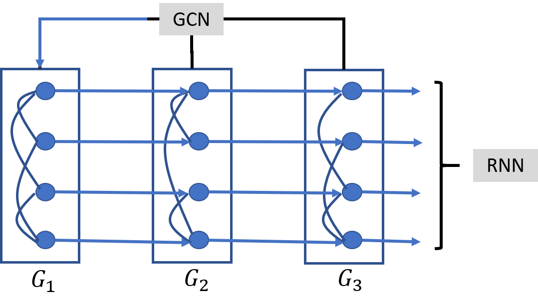
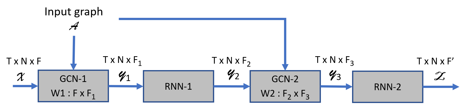
(a) GCN and RNN operations		(b) Multi-layer dynamic GNN

Figure 1: Dynamic GNN. Part (a) illustrates a single pair of GCN and RNN operations over $N=4$ vertices and $T=3$ timesteps. Part (b) presents a two layer model with each layer consisting of a GCN-RNN pair.

Dynamic Graph Neural Networks for DTDG. Our work applies to a family of dynamic GNN models for DTDGs, which we abstract using the framework described below. Details specific to the three representative models (TM-GCN, CD-GCN, EvolveGCN) used in our experimental evaluation are described in Section 5.

Under the framework, a dynamic GNN model consists of multiple layers. Each layer involves a GCN [11] module operating on each snapshot independently, followed by an RNN module operating on the feature-vector of each vertex independently along the timeline. Figure 1 (a) illustrates the idea.

A multi-layer model is constructed by iterating over this pair of GCN/RNN operations. Figure 1 (b) illustrates a two-layer model. Here, the input dynamic graph is represented as a sparse tensor ${\cal A}$ of size $T\times N\times N$, and the input features ${\cal X}$ is a dense tensor of size $T\times N\times F$. Tensor notation is used to represent the intermediate activations as well. While the two RNN components operate on the intermediate features output by the previous module, the GCN components apply graph convolution on the input dynamic graph.

The intermediate feature lengths $F_{1},F_{2},F_{3}$, and the embedding length $F^{\prime}$ are tunable. They determine the size of the GCN weight matrices and the internal parameters of the RNN. The output of the iterative process is a tensor ${\cal Z}$ of size $T\times N\times F^{\prime}$ that provides an embedding of size $F^{\prime}$ for each $u$ at each timestep $t$.

The embeddings can be used in multiple ways. In vertex classification, we are given ground truth labels for each vertex at each timestep in the form of a matrix $Q$ of size $T\times N$ with entries from $\{1,\ldots,C\}$, where $C$ is the number of categories. For this application, we derive predictions by projecting each embedding matrix $Z_{t}$ to the label space via a learnable weight matrix $U$ of size $F^{\prime}\times C$. The predictions are compared against the ground truth using a loss function such as cross-entropy. Edge prediction can be performed via concatenating the embeddings of the edge end-points. The latter is explored in our experimental evaluation.

The weight matrices associated with the GCN and the RNN modules, and the matrix $U$ are the learnable parameters of the model. Backpropagation of the gradients is performed after the forward phase has completed the processing of all the snapshots (all their vertices).

Figure 2: Gradient checkpoint illustration. Here, number of blocks ${\tt nb}=3$. $\pi_{j}$ represents the RNN-specific data passed from block $j$ to $j+1$, which gets stored as part of checkpointing. $\pi_{0}$ is the initial data.

3 Single GPU Implementation

In this section, we discuss optimizations of gradient checkpoint and graph-difference based CPU-GPU transfer.

3.1 Gradient Checkpoint

The standard two-phase training process, consisting of forward and backpropagation, involves storing a copy of the intermediate activation tensors, as well as the inputs ${\cal A}$ and ${\cal X}$. This leads to severe GPU memory bottleneck for large inputs. In our experiments, most of the model-dataset configurations do not execute on fewer than $8$ GPUs. We adapt the well-known gradient checkpoint method (e.g., [4, 6]) to optimize the memory requirements.

In our setting, the GCN component operates independently on each snapshot, but inter-dependency is caused by the RNN component acting along the timeline. We partition the timeline into ${\tt nb}$ blocks, each containing ${\tt bsize}=T/{\tt nb}$ timesteps, where the number of blocks ${\tt nb}$ is a tunable parameter. For a block $b\in[1,{\tt nb}]$, the range of timesteps is given by the starting and ending timesteps $s(b)=1+(b-1)\cdot{\tt bsize}$ and $e(b)=b\cdot{\tt bsize}$.

The idea of checkpointing is to restrict the storage of the input and the intermediate data to a single block at any point during the execution. Towards that goal, we first execute the forward pass in the usual manner by processing the blocks in the increasing order. Then, the backpropagation pass is conducted in the reverse order, starting with the last block. The processing of each block $b$ consists of two parts: a rerun of the forward pass, followed by gradient propagation in the reverse direction. The process limits the memory usage to a single block thereby reducing the overall the memory requirement. See Figure 2 for an illustration.

The procedure requires the ability to re-execute a block $b$. The GCN component does not have dependency on the prior block $b-1$. However, the RNN component requires the following data computed in block $b-1$: (i) the RNN hidden state corresponding to the last timestep of block $b-1$ (namely $S_{e(b-1)}$); (ii) the activations of the RNN corresponding to the last $w$ timesteps of the block $b-1$, where $w$ is the window size (see Eqn. 3). We denote the above information passed from block $b-1$ to block $b$ as $\pi_{b-1}$ (see Figure 2). We store $\pi_{b}$ for all the blocks during the forward pass, to be reused during backpropagation.

The total GPU memory requirement involves two components: memory needed to store the activations of the current block and the checkpoint data. The former consists of the snapshots $A_{s(b)},\ldots,$$A_{e(b)}$, input features $X_{s(b)},\ldots,X_{e(b)}$, and the intermediate tensors. The latter consists of the checkpoint data $\pi_{b}$ stored across all the blocks. While the former intra-block memory requirement is determined by the block size ${\tt bsize}=T/{\tt nb}$, the checkpoint data is determined by the number of blocks ${\tt nb}$. The two components can be balanced by adjusting the parameter ${\tt nb}$.

The parameter ${\tt nb}$ not only determines GPU memory usage, but also influences the execution time, since the GPU utilization is better and the latency is lower under larger block sizes (fewer blocks). In our experiments, we tune the parameter so as to achieve the best possible execution time, while ensuring that the GPU memory usage does not exceed the available memory.

3.2 Graph-difference Based Input Transfer

In order to save memory, our checkpoint implementation stores only the input and the intermediate data corresponding the current block $b$ in the GPU. While latter gets generated and resides on the GPU, the input comprising of the snapshots and the features corresponding to the block $b$ get transferred from the CPU to the GPU. This transfer happens twice, once during the forward phase and the second during the rerun segment of the backpropagation. We use pinned memory to optimize the above data transfer, as this avoids the use of paged memory. In spite of the optimization, our experiments show that the transfer time constitutes an important component of the overall execution. In this section, we exploit the properties of dynamic graphs to devise a graph-difference based method that reduces the transfer time.

Our method is motivated by the fact that dynamic graphs change gradually and therefore consecutive snapshots are expected to have substantial overlaps in their topology. In addition, as explained later (c.f. Section 5), towards improving accuracy, TM-GCN and EvolveGCN apply certain pre-processing steps, named M-product and edge-life. These steps tend to smoothen the differences across the snapshots, and as a result, they magnify the overlaps in the topology among consecutive snapshots.

Consider a block $b$ pertaining to the sequence of snapshots$A_{s(b)},\ldots,A_{e(b)}$ of length ${\tt bsize}$. The first snapshot $A_{s(b)}$ is transferred from the CPU to the GPU using standard sparse matrix representation of (index,value) pairs. Consider two consecutive snapshots $A_{i}$ and $A_{i+1}$. Assuming that $A_{i}$ is already present in GPU, we describe how the graph-difference method transfers $A_{i+1}$.

We partition the edges of $A_{i}$ and $A_{i+1}$ into three sets:

• $A^{com}$: the set of common edges present in both $A_{i}$ and $A_{i+1}$,

• $A_{i}^{ext}$: the extra edges present in $A_{i}$ but not in $A_{i+1}$, and

• $A_{i+1}^{ext}$: the extra edges present in $A_{i+1}$ but not in $A_{i}$.

Now, instead of transferring $A_{i+1}$ using standard sparse matrix representation, we only transfer:

• the indices corresponding to $A_{i}^{ext}$

• the indices corresponding to $A_{i+1}^{ext}$

• all the values for the new snapshot $A_{i+1}$

We first derive the common indices $A^{com}$ by excluding $A_{i}^{ext}$ from $A_{i}$. We then reconstruct the indices of the new snapshot $A_{i+1}$ by adding the extra edges in $A_{i+1}^{ext}$ to $A^{com}$. While the snapshots overlap in terms of the topology, the values associated with their edges are not expected to overlap. So, the transfer of value of the new snapshot is required. When there is a large overlap in the structure, this results in substantial saving as it avoids transferring the indices for the common structure of the snapshots $A_{i}$ and $A_{i+1}$.

4 Distributed Implementation

In the multi-node setting, the communication volume is a critical aspect and it is determined by the data partitioning. We first discuss a vertex partitioning approach, adapted from the static GNN setting, and then present our snapshot partitioning approach. Assume that we have $P$ processors, each endowed with a GPU, which could be cores of the same node or span multiple nodes.

4.1 Vertex Partitioning Approach

A common approach used in (static) GNN setting with a single input graph is to partition the vertices among the processors (e.g, [31]). Adapting to our setting, we partition the vertex set $V$ uniformly among the processors so that each processor $p$ owns $N/P$ vertices, denoted $V_{p}$. The snapshots get partitioned accordingly: for each $t$, the rows of $A_{t}$ corresponding to $V_{p}$ are stored at processor $p$. Each input feature matrix $X_{t}$ is partitioned in a similar manner.

The RNN component operates independently on each vertex. Hence, each processor $p$ can perform the operation on the set of vertices $V_{p}$ without having to communicate with the other processors. Thus, the RNN component is communication free. However, the GCN component requires significant communication.

Consider the GCN operation on a snapshot $A_{t}$. Each vertex $u$ aggregate the neighborhood features. Viewed from the other direction, the feature of a vertex $v$ is required by all its neighbors $\Gamma_{t}(v)$, which may be distributed among multiple processors. Let $\lambda_{t}(v)$ denote the number of processors that own at least one neighbor of $v$. Then, the communication is $\lambda_{t}(v)$ units. Summed across all snapshots and vertices, the total communication is given by $\sum_{t}\sum_{v}\lambda_{t}(v)$ units per GCN module, where a unit refers to a feature vector. The partition minimizing the above communication volume can be found using hypergraph partitioners such as PaToH [2].

Shortcomings of Vertex-partitioning. Under vertex partitioning, the communication volume increases with the number of processors $P$ and is dependent on the graph density. In addition, the communication pattern is irregular, resulting in significant implementation overheads. Finally, the approach requires sophisticated hypergraph partitioners that incur high preprocessing time. Similar observations have been made in recent prior work on scaling GNN [23]. The dynamic GNN allows us to design simpler and effective partitioning algorithm that overcomes the above issues.

4.2 Snapshot Partitioning and Redistribution

The core idea of our scheme is to partition the snapshots among the processors, instead of the vertices. We then accommodate the RNN component via a re-distribution of the feature matrices.

(a) Non-checkpoint setting

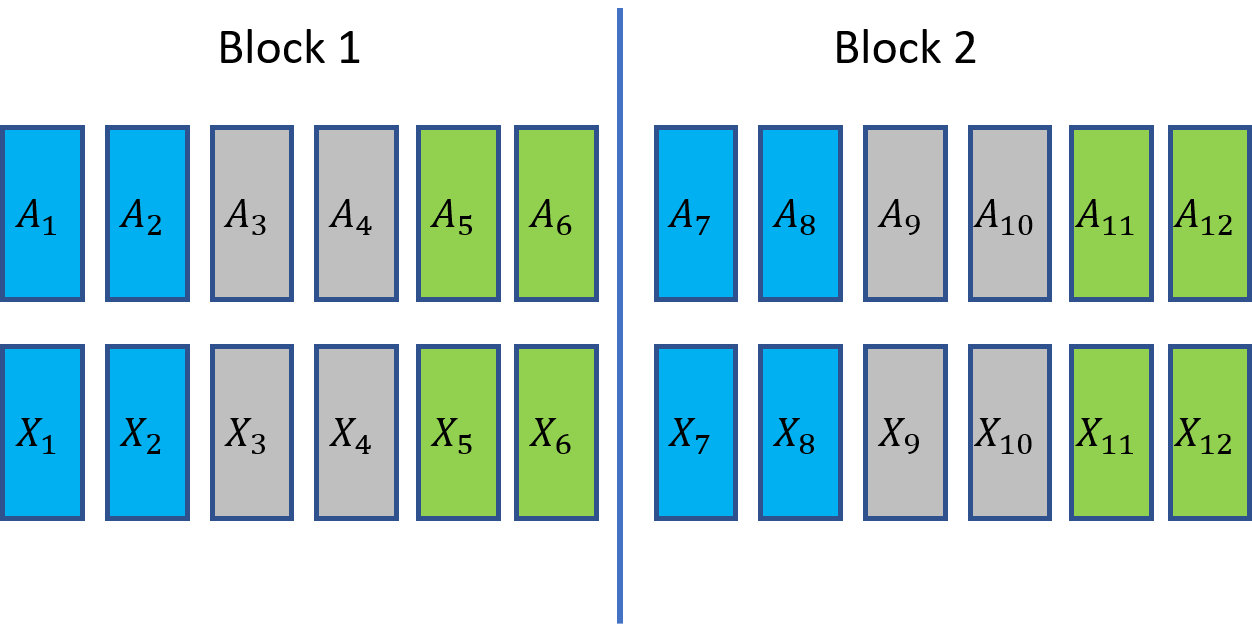
(b) Checkpoint setting

Figure 3: Snapshot partitioning and re-distribution. Part (a) illustrates the process without checkpoint taking $T=6$ timesteps and $P=3$ processors, represented by the three colors. The matrices $A_{t}$ are sparse and are of size $N\times N$, whereas the other matrices are feature matrices of size $N\times F$ (with different feature lengths $F$). The figure shows the partitioning of the snapshots $A_{t}$ and the input features $X_{t}$, as well the two re-distributions and the GCN/RNN operations. Part (b) illustrates the partitioning in the checkpoint setting taking $T=12$, $P=3$ and the number of blocks ${\tt nb}=2$.

Snapshot Partitioning and GCN. For the ease of exposition, we first discuss the implementation without gradient checkpoint. Consider the first layer of the model involving a pair of GNN and RNN components. Figure 3 (a) illustrates the partitioning and the execution of the GCN/RNN components described below.

We partition the snapshots among the processors in a contiguous manner so that each processor owns $k=T/P$ contiguous snapshots. Namely, processor $p$ is assigned snapshots $A_{s}$ to $A_{e}$, where $s=1+(p-1)\cdot k$ and $e=p\cdot k$. Similarly, the input features $X_{s}$ to $X_{e}$ are assigned to $p$. The GCN weight matrices $W$ are very small in size and we store a copy of the matrices in all the processors.

For each $t$, the processor responsible for the timestep $t$ has both $A_{t}$ and $X_{t}$ in entirety, and so it can perform the GCN operation $Y_{t}=\widetilde{A}\cdot X_{t}\cdot W$ by itself without communication. Thus, the GCN component is communication free. Let $Y_{1},Y_{2},\ldots,Y_{T}$ denote the output matrices of the GCN operation, where $Y_{t}$ is generated at the processor responsible for the timestep $t$.

Re-distribution and RNN. The RNN module is applied over the sequence $Y_{1},Y_{2},\ldots,Y_{T}$. The module operates on each vertex $u$ independently and requires the entire sequence $Y_{1}[u],Y_{2}[u],\ldots,Y_{T}[u]$, due to dependency across the timeline. To facilitate the process, we re-distribute the matrices by performing a vertex-level partitioning. We partition the vertex set $V=\{v_{1},v_{2},\ldots,v_{N}\}$ into $P$ chunks of size $k=N/P$ each and make processor $q$ the owner of the $q^{th}$ chunk. Namely, the processor $q$ owns the vertices $V_{q}=\{v_{s},\ldots,v_{e}\}$, where $s=1+(q-1)\cdot k$ and $e=q\cdot k$.

For each timestep $t$, the processor $p$ responsible for the timestep splits the matrix $Y_{t}$ into $P$ chunks and sends the $q^{th}$ chunk to the processor $q$. The processor $q$ assembles the sequence $Y_{1}[V_{q}],Y_{2}[V_{q}],\ldots,Y_{T}[V_{q}]$ and applies the RNN operation. The data transfers are realized via an all-to-all communication.

Let the output of the operation be $Z_{1}[V_{q}],\ldots,Z_{T}[V_{q}]$. The dynamic GNN model may involve multiple layers. To prepare for the GCN model at the next layer, we re-distribute the $Z$ matrices to match the original snapshot partitioning. Namely, for each $q$ and $t$, the processor $q$ sends $Z_{t}[V_{q}]$ to the processor $p$ responsible for timestep $t$. Upon receiving the data, each processor $p$ can reassemble the matrix $Z_{t}$ for each timestep it is responsible for. As before, the data transfers are realized via an all-to-all communication.

Gradient Checkpoint Implementation. We next adapt the partitioning algorithm to the context of gradient checkpoint. Assume that we have ${\tt nb}$ blocks each having ${\tt bsize}=T/{\tt nb}$ timesteps. We apply snapshot partitioning within each block so that each processor is responsible for ${\tt bsize}/P$ timesteps within the block. Consequently, snapshots assigned to a processor are contiguous within a block, but non-contiguous when viewed over the entire timeline. See Figure 3 (b) for an illustration.

The above block-wise partitioning facilitates the RNN computation. The processors operate within the same block and move to the next in a synchronous fashion. For each block, the GCN operations are applied over the timesteps in the block and the RNN operation is executed restricted to the block. Similarly, the all-to-all communication are also limited to feature matrices of the block. Finally, checkpoint data is stored and the procedure advances to the next block.

Communication Volume. For every dynamic GNN layer consisting of a GCN-RNN pair, we perform two re-distributions. Each involves an all-to-all communication with an overall volume of $T\cdot N$ units, where a unit refers to a feature vector. Regarding backpropagation, at a high level, the procedure is executed in a symmetrically opposite manner via performing the above steps in the reverse order. Akin the to the forward phase, the procedure involves two gradient re-distributions, realized via all-to-all communications. Thus, the overall communication volume is $O(T\cdot N)$ units.

Advantages of Snapshot Partitioning. An important benefit of snapshot partitioning is that the the communication volume is fixed at $O(T\cdot N)$ units, for any number of processors and irrespective of the graph density properties. Furthermore, the partitioning and the communication follow a regular pattern, which combined with the simplicity of the scheme, results in minimal implementation overheads. These factors lead to better scalability. Finally, the scheme does not require sophisticated hypergraph partitioners and has limited preprocessing cost.

5 Dynamic GNN Architectures

We describe the three models used in our experimental study. They are representative of the dynamic GNN models for DTDG known from prior literature (see survey [9]), making our optimization techniques applicable to the current state of the art. All the three models follow the framework described in Section 2.2, but differ in the choice of the RNN component.

5.1 CD-GCN

The Concatenate Dynamic GCN [17] uses the well-known LSTM [7] for RNN temporal aggregation. At a high level, referring Equation 3, LSTM state $S_{t}$ consists of a pair $(h_{t},c_{t})$ referred as the hidden and the cell memory. At timestep $t$, the state $S_{t}$ and the output $Y_{t}$ are derived from the previous state $S_{t-1}$, the current input $X_{t}$ and the previous output $Y_{t-1}$. Thus, the LSTM maintains a window length of $w=1$.

Based on accuracy considerations, CD-GCN incorporates skip-connection to GCN by concatenating the input features to the output, via modifying Equation (2):

$$Y_{0}=\widetilde{A}\cdot X,\quad\quad Y_{1}=Y_{0}\cdot W,\quad\quad Y=\sigma(Y_{0}\circ Y_{1}),$$

where $Y_{0}\circ Y_{1}$ represents concatenation. As a result, $Y$ will have $F+F^{\prime}$ features. The CD-GCN as proposed in [17] comprises of a single dynamic GNN layer given by a GCN-LSTM pair. We extend this architecture to two layers in the interest of generality of our study. This will allow similar deeper models, to make use of our acceleration strategies.

5.2 EvolveGCN

The evolving GCN [19] model also uses LSTM, but incorporates two interesting aspects. First, it maintains a different GCN weight matrix $W_{t}$ for each timestep $t$ so that Equation 2 is modified as:

$$Y_{t}=\sigma(\widetilde{A_{t}}\cdot X_{t}\cdot W_{t}).$$

Secondly, instead of applying LSTM over the vertex features of the graph, the model applies LSTM over the weight matrices. Each layer therefore performs the following operations:

$$W_{t}=LSTM(W_{t-1}),$$

$$Y_{t}=GCN(A_{t},X_{t},W_{t}),$$

Intuitively, the weights evolve over the timeline and directly imbibe the temporal properties. The paper offers two variants namely, EGCN-O and EGCN-H. The above model corresponds to EGCN-O.

5.3 TM-GCN

In contrast to CD-GCN and EvolveGCN, for the RNN component, the TM-GCN model employs M-transform [10], a parameter-less temporal aggregation mechanism. Given input features $X_{1}[u],\ldots,X_{T}[u]$ for a vertex $u$, the output sequence $Y_{1}[u],\ldots,Y_{T}[u]$ is obtained by aggregating the current and the previous $w$ input features at each timestep $t$:

$$Y_{t}[u]={\tt aggregate}(X_{t-w}[u],\ldots,X_{t}[u]),$$

where $w$ is the tunable window size and aggregation is weighted averaging.

Equivalently, the M-transform can be expressed in terms of tensor operations. Let $M$ be a $T\times T$ lower diagonal matrix. Given an input tensor ${\cal X}$ of size $T\times N\times F$, the M-transform is given by: ${\cal Y}={\cal X}\times_{1}M$, where $\times_{1}$ refers to the first-mode tensor-times-matrix (TTM) product. The output tensor ${\cal Y}$ has same size as ${\cal X}$. The temporal effect is restricted to the prior $w$ steps by defining $M$ as:

$$M_{tk}=\begin{cases}\frac{1}{min(w,t)}&\quad\text{if}\max(1,t-w+1)\leq k\leq t,\\ 0&\quad\text{otherwise.}\\ \end{cases}.$$

The choice of weights result in averaging and normalizing the features over the timeline.

5.4 Smoothening the Input Graphs

Real world dynamic graphs tend to be extremely sparse. Towards increasing the density and to maintain continuity over consecutive snapshots, EvolveGCN and TM-GCN smoothen the snapshots via the notion of edge-life and M-transform, respectively.

The edge-life transformation carries edges from each snapshot to the subsequent $l$ snapshots by modifying each $A_{t}$ as:

$$A_{t}=A_{t}+\sum_{i=t-l+1}^{t-1}A_{i},$$

where the parameter $l$, called edge-life, is a tunable parameter. The transformation introduces changes into the graph topology at a slower pace and increases the density as well.

The TM-GCN model implements smoothening by applying the M-transform to the input tensor ${\cal A}$, as well the input feature tensor ${\cal X}$. In practice, the two mechanisms achieve similar smoothing effect and both are applied in a pre-processing step.

5.5 Implementation Aspects

Our implementation of the three models follows a common framework incorporating graph-difference and snapshot-partitioning. Below, we highlight implementation aspects specific to the models.

The EvolveGCN model maintains a separate GCN weight matrix $W_{t}$ for each timestep. These matrices are small in size and we store copies in each processor. The model applies the LSTM operation over the above weight matrices, as against the feature matrices. Consequently, the LSTM operation can be executed by each processor without having to communicate with the other processors. Thus, in addition to GCN, the LSTM component also becomes communication free. To rephrase, each processor acts independently on on the snapshots assigned to it. The backpropagation is also executed in a similar manner and partial gradients for the model parameters are derived. At the end of the training epoch, these gradients are aggregated across the processors via an all-reduce operation. This constitutes the only communication and the volume is insignificant since the weight matrices are small in size. The M-transform based smoothening used in TM-GCN is also executed as pre-processing.

For all the three models, we optimize the spatial aggregation of the first GCN layer via pre-computation. The GCN operation (Equation 2) can be split as $Y^{\prime}=\widetilde{A}\cdot X$ and $Y=Y^{\prime}\cdot W$. Notice that the first part is independent of any model parameters. So, we pre-compute the product and reuse the result in each training epoch. Since the operation is an expensive sparse-dense mulitplication, this pre-processing improves training time for the baseline as well.

	N	T	nnz	M-product	edge-life
epinions	755 K	501	13 M	653 M	1038 M
flickr	2.3 M	134	33 M	963 M	796 M
youtube	3.2 M	203	12 M	851 M	802 M
AMLSim	1 M	200	124 M	1094 M	1038 M

Table 1: Datasets. For each dataset, the number of vertices ($N$), timesteps ($T$), total number of edges or non-zero elements (nnz) across all the snapshots are shown. TM-GCN and the EvolveGCN smoothen the input graph by applying M-product and edge-life, which introduces new non-zero elements. The number of non-zero elements after each of the operations is given in the last two columns. The two models are trained on the respective smoothened graphs.

6 Experimental Evaluation

In this section, we present an experimental evaluation, first focusing on our CPU-GPU optimizations and snapshot-partitioning, followed by a preliminary comparison to the vertex-partitioning approach. While snapshot-partitioning offers better scaling, it has certain limitations when the individual snapshots are large. We briefly describe possible strategies for addressing them.

6.1 Setup

System. The experiments were conducted on the AiMOS system (https://cci.rpi.edu/aimos). Our setup uses $16$ nodes, each with $8$ GPUs, leading to a total of $128$ GPUs. Each node has 2x20 cores of 2.5GHz Intel Xeon Gold 6248 and has 768 GiB RAM (shared by the $8$ GPUs). Each GPU is NVIDIA Tesla V100 with 32 GiB HBM. The nodes are connected by Dual 100 Gb EDR Infiniband. In each node, we run up to $8$ processes, each controlling a single GPU and mapped to a separate core of the node. We use PyTorch 1.7.1 for training, NCCL 2.8.4 for backend communication and PyNCCL 0.1.2 for collective routines. All our codes are implemented in python.

Dataset. Our benchmark consists of four datasets shown in Table 1. Epinions is derived from a user-product rating system, wheres Youtube represents user-user links and Fickr is based on links among images. The edges for each of these datasets are timestamped with the time at which the links are formed. All the three datasets were obtained from Networks Repository [21]. AML-Sim is generated from an Anti-money laundering simulator [26]. The metadata for these datasets is shown in Table 1. As discussed earlier (Section 5), TM-GCN and EvolveGCN smoothen the input graphs by applying the M-product and the edge-life operations in a preprocessing step. The process increases the size (number of edges) of the snapshots. The sizes of the input and the smoothened graphs are shown in the table. The models are trained on the respective smoothened graphs. For instance, for the AMLsim graph, TM-GCN is trained on a graph of size $1094M$ edges.

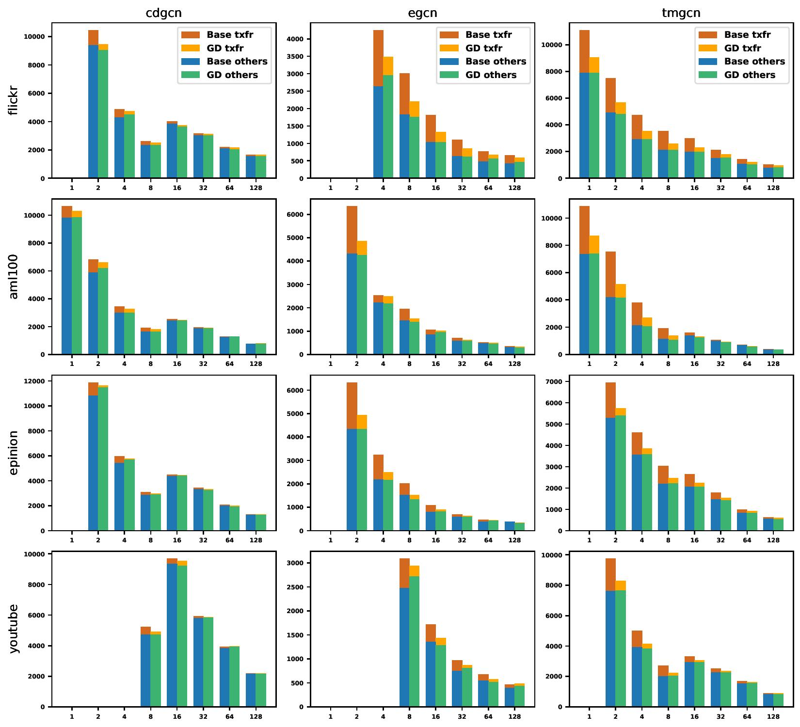
Figure 4: Evaluation of graph-difference technique. Comparison of the naive baseline (Base) and the graph-difference (GD) snapshot transfer methods are shown for each dataset-model pair. In all the plots, X-axis is the number of GPUs and Y-axis is the execution time in milliseconds. Each datapoint is split into two components: the transfer time, and others, which includes the computation and communication time. In some cases, the models did not execute on small number of GPUs due to insufficient memory and these are left blank.

Models and Evaluation. We evaluate our optimization techniques on three representative dynamic GNN models: CD-GCN [17], EvolveGCN [19] and TM-GCN [16]. For all the model-dataset configurations, we use the in and out degrees as the input features, as done in TM-GCN [16]. The intermediate feature lengths are set to $6$ and the number of classification categories is $2$.

As discussed earlier (Section 2.2), the dynamic GNN models generate vertex-level embeddings. Edge-level embeddings can be derived by concatenating the embeddings of $u$ and $v$ for each edge $(u,v)$. These embeddings can be used in different ways depending on the task under consideration such as vertex classification and link prediction. The first part of our study is concerned with analyzing the running time performance of our optimization strategies and snapshot-partitioning. For this purpose, we measure time taken for generating the embedding (and the corresponding backpropagation) per training epoch, averaged over $5$ epochs. The subsequent segment of the study compares snapshot-partitioning with vertex-partitioning, which includes an analysis of the loss/accuracy convergence behavior. For this purpose, we consider the specific task of link prediction.

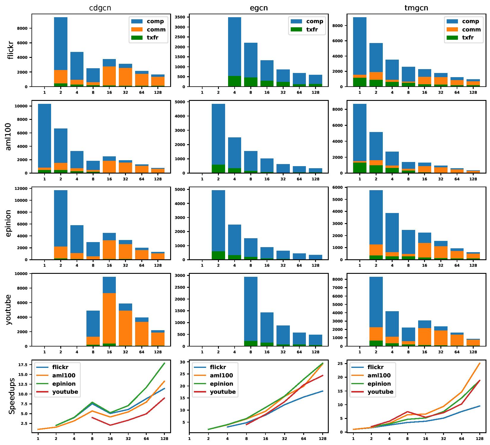
Figure 5: Strong scaling. Results for each dataset-model pair is shown. The implementation is endowed with the GD technique for snapshot transfer. The X-axis is the number of GPUs and Y-axis is the execution time in milliseconds. Each datapoint is split into three components: the transfer time, computation time and the communication time. For each model, the last plot provides a summary containing the speedup on all the datasets for different values of $P$ with respect to $P=1$ as the reference. For configurations where a single processor could not execute due to insufficient GPU memory, the smallest number of processors $P$ where the execution completed is taken as the reference. Since the reference point $P$ varies across different datasets, for ease of comparison, we take the speedup at $P$ processors as $P$.

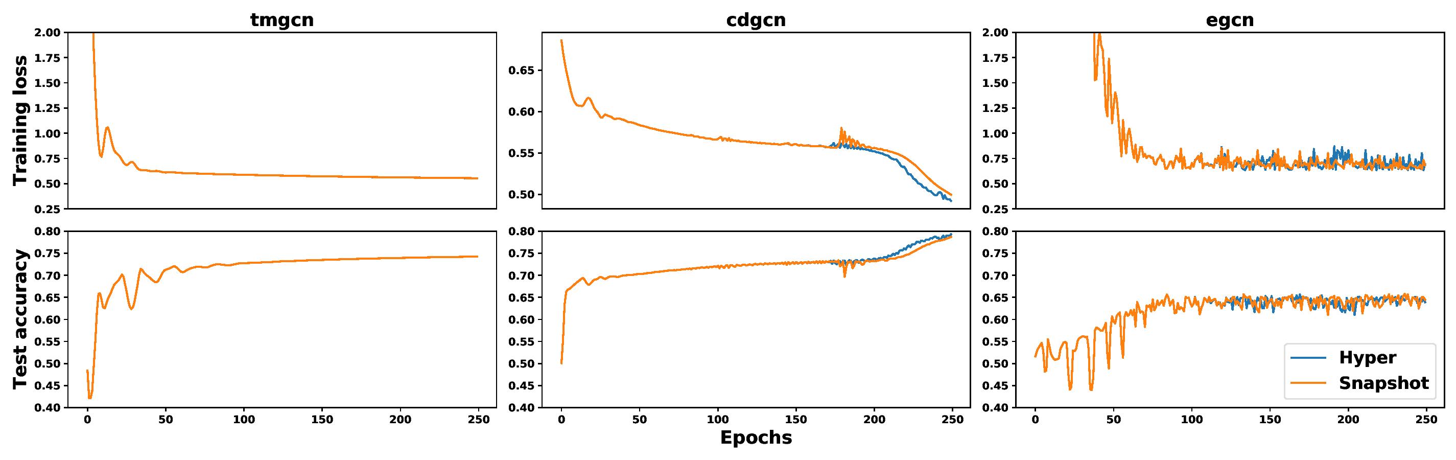
Figure 6: Loss and test accuracy convergence under snapshot and hypergraph partitioning schemes for the three models on the AML-Sim dataset. The curves for TM-GCN are identical.

6.2 Checkpoint and Graph Difference

We first evaluate the baseline and the checkpoint based implementations. Across different model-dataset configurations, we found that the baseline did not execute on a single node, endowed with $8$ GPUs, due to GPU memory bottleneck. In contrast, the checkpoint based implementation was able to successfully run on a single node for all the configuration, with even lesser than $8$ GPUs.

As discussed earlier (Section 3.1), the checkpoint based implementation needs to transfer adjacency matrices $A_{s(b)},\ldots,A_{e(b)}$ from CPU to GPU while executing a block $b$. This can be accomplished via naively transferring the matrices in sparse representation given by indices and values. In contrast, our graph-difference based technique saves execution time by transferring only the difference of each snapshot with respect to the previous snapshot. We use pinned memory to optimize the both the methods as it avoids the use of paged memory.

We denote the naive baseline method as Base and the graph difference method as GD. We evaluate the performance of the two methods on all the dataset-model pairs for number of processors $P=1$ to $128$. The results are shown in Figure 4. For the ease of comparison, we divide the overall execution time into two components: (i) the snapshot transfer time; (ii) others, which includes computation and inter-GPU communication.

We can see that for the EvolveGCN and TM-GCN models, GD provides significant reduction in the transfer time across the datasets, with the speedup factors as high as $4.1$x. As a result, the overall execution time improves by up to $40\%$. As discussed earlier (Section 5), based on accuracy considerations, the two models smoothen the input snapshots by applying the edge-life and the M-product operations to the input snapshots. These operations magnify the similarity among consecutive snapshots, enhancing the gains for GD. In contrast, CD-GCN works directly with the input snapshots and the gains in transfer time are up to $2$x. The latter result demonstrates the strong similarity among the snapshots in real-life, which can possibly be exploited in other contexts as well.

We can see that the gains are higher at smaller GPUs, and this is due to the checkpoint mechanism. The checkpoint based implementation executes one block at a time. The first snapshot of each block is transferred naively and the rest of the snapshots are transferred via the GD method. Thus, the fraction of the snapshots that benefit from GD is given by $({\tt bsize}-1)/{\tt bsize}$, where ${\tt bsize}$ is the number of timesteps in each block. In the multi-GPU setting, each block is partitioned uniformly, with each processor receiving ${\tt bsize}_{p}={\tt bsize}_{p}/P$ snapshots. The requirement of naively transferring the first snapshot applies within the chunk of snapshots assigned to each processor. Consequently, the fraction of snapshots that benefit from GD becomes $({\tt bsize}_{p}-1)/{\tt bsize}_{p}=({\tt bsize}-P)/{\tt bsize}$. As the number of processors $P$ increases, the benefit ratio decreases. Furthermore, communication becomes more dominant at higher system sizes. Consequently, the GD technique provides higher gains for smaller number of GPUs. In summary, the checkpoint and the graph-difference mechanisms allow efficient execution of large datasets on a single node.

6.3 Scaling Study

Strong Scaling. We next study the strong scaling behavior of the implementation, endowed with the GD technique for snapshot transfer. The results are shown Figure 5. As before, the results for each dataset-model pair is presented. The plots provide breakup of the execution time in terms of three components: snapshot transfer, computation and communication. Apart from the detailed breakup, for each model, a summary plot is included which presents the speedup curves for all the datasets. Taking $P=1$ as the reference point, the plot provides the speedup achieved as we increase the number of processors to $128$.

As discussed in Section 5, the communication volume EvolveGCN is insignificant for EvolveGCN, and so, only the other two components are shown. As $P$ increases, each processor handles lesser number of snapshots and hence, the computation time scales well for all the dataset-model configurations.

In contrast, the communication becomes a bottleneck for TM-GCN and CD-GCN at higher number of processors. Under snapshot partitioning, the communication volume is $O(T\cdot N)$, irrespective of the number of processors $P$. However, the communication time depends upon the system size. Each node has $8$ GPUs and so for $P\leq 8$, the communication is intra-node and does not involve interconnection network. Higher number of processors require inter-node communication and as a result, we observe a drop in speedup at $P=16$ compared to $P=8$. On further analysis, note that the fraction of intra-node volume is $1/K$ and the inter-node volume is $(K-1)/K$, where $K=P/8$ is the number of nodes. Thus, the inter-node volume increases with the number of nodes. On the other hand, the bisection bandwidth increases with $K$. The combination of the two aspects determine the communication time and the scaling behavior improves as $K$ increases. At $P=128$, the speedup is up to $30$x, as against the ideal value of $128$x.

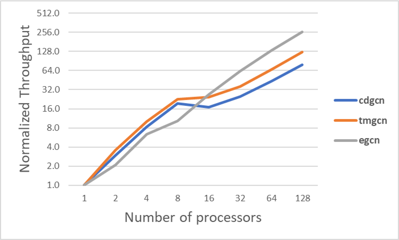
Figure 7: Weak scaling of the three models.

Weak Scaling. We next study the weak scaling behavior using randomly generated graphs. Given $T$, $N$ and edge density $f$, the generator constructs each snapshot independently by adding $N$ vertices and randomly selecting $m=N\cdot f$ pairs of vertices as edges. The edge-life and the M-product operations are applied to the graphs in the case of EvolveGCN and TM-GCN models, respectively.

We set the number of timesteps $T=256$ and edge density $f=3$. Starting with $N=2^{14}$ at $P=1$, we scale up to $P=128$ processors via doubling $N$ at each step, so that the number of vertices is $1M$ at $P=128$. In the case of TM-GCN, the aggregate number of edges across the snapshots (after M-product) varied from $16M$ to $2.1B$ for TM-GCN and the other models showed similar trend.

The results are shown in Figure 7. We compute the throughput as the ratio of aggregate number of edges across all the snapshots to the execution time. We derive the speedup by normalizing the throughput with respect to $P=1$ for each model. We can see that TM-GCN and CD-GCN achieve a speedup of $125$x and $79$x at $P=128$, as against the ideal value of $128$. The scaling briefly drops going from $P=8$ to $P=16$. The reason is that each node has $8$ GPUs, and hence the node boundary is crossed at $P=16$, resulting in the use of slower inter-node communication links. The EvolveGCN model involves communication only for gradient aggregation and achieves superlinear speedup of $260$x at $P=128$.

6.4 Comparison with Vertex-Partitioning

We present a preliminary empirical comparison of our snapshot-partitioning scheme with the vertex-distribution method based on hypergraph partitioning (Section 4.2), illustrating the benefits of snapshot-partitioning discussed therein. While hypergraph-based partitioning has been well studied in the context of graph processing and static GNN, no prior implementation is available for our dynamic GNN setting. Towards enabling the study, we developed a basic implementation of the strategy.

Vertex-Partitioning Implementation. We use PaToH [2] hypergraph partitioner to determine the set of vertices $V_{p}$ owned by each processor $p$. The vertices $V_{p}$ need not be consecutive, but we make them to be consecutive via renaming, to avoid implementation overheads. At each timestep $t$, the $N\times N$ Laplacian sparse matrix $\widetilde{A}_{t}$ and the $N\times F$ feature matrix $X_{t}$ are distributed by assigning the sub-matrices $\widetilde{A}_{t}[V_{p},:]$ (rows corresponding vertices in $V_{p}$) and $X_{t}[V_{p},:]$ to the processor $p$. Since RNN operates on each vertex independently over the timeline, it can be executed via kernel calls without the need for communication. However, the SpMM convolution operation $Y_{t}=\widetilde{A}_{t}\cdot X_{t}$ is more involved and requires communication. We want the result $Y_{t}$ to be distributed in the same manner so that $p$ derives $Y_{t}[V_{p},:]$. In this computation, $p$ requires the row $X_{t}[v,:]$, for a vertex $v$, only if the corresponding column $\widetilde{A}_{t}[:,v]$ contains at least one non-zero element (alternatively, $p$ owns a neighbor of $v$). To reduce the communication, any processor sends only the required rows to the other processors. The hypergraph partitioner is set up in a such a manner that the above communication volume is minimized. To avoid overheads during training time, the indices are pre-computed so that each processor knows the rows it needs to send to every other processor. Our implementation ensures that data structures such as the above indices are maintained in-place on the GPU.

Link Prediction. For the purpose of comparing the two partitioning schemes, we study the link prediction problem considered in prior work on dynamic GNN [16, 19]. The objective is to train on the first $T$ timesteps and predict edges that might appear on timestep $T+1$. To construct the training set, for each timestep, we select $\theta$ fraction of the edges in $G_{t}$ and assign them label $1$, and include an equal number of randomly chosen vertex-pairs $(u,v)$, with label $0$. The testing sample at timestep $T+1$ is constructed in a similar manner from the graph $G_{T+1}$. The test accuracy is measured as the percentage of correctly classified pairs. The parameter $\theta$ controls the size of the training set and we set it to $0.1$ in our experiments. The dynamic GNN models produce an embedding for each vertex at each timestep. We derive classification for a pair of vertices $(u,v)$ by concatenating the embedding of the two endpoints and applying a fully connected layer.

Evaluation. We illustrate the benefits of snapshot partitioning by considering the AML-Sim dataset. We execute all the three models on this dataset under the two partitioning schemes. We provide the gradient checkpoint mechanism to hypergraph partitioning as well, to avoid GPU memory bottlenecks. Snapshot-partitioning is endowed with the graph-difference based CPU-GPU transfer of snapshots, whereas the hypergraph partitioning transfers the snapshots directly. We execute GCN and RNN as single-batch operations. The results of the evaluation are shown in Table 2 (averaged over five epochs).

Loss Convergence. Before analyzing the execution time performance, we first consider the convergence of loss and accuracy under the two partition schemes. Unlike deep neural networks, our processing does not involve (variable sized) batched gradient descent or batch normalization layers that impact final accuracy. Consequently, both the schemes simulate the underlying sequential algorithms faithfully. As a result, their convergence behaviors are identical, except for floating point accumulation errors. This is illustrated by Figure 6, which shows the cross-entropy loss and test accuracy for the two schemes. We can see that the curves are identical under the two schemes for the TM-GCN model, and diverge mildly towards the end for CD-GCN. There is noticeable differences on EvolveGCN, however the underlying (sequential) loss and accuracy in this case show considerable fluctuations within consecutive epochs. Given that the two models simulate the convergence of the sequential model, we can compare their execution time performance on a per-epoch basis.

Communication Volume. Snapshot-partitioning incurs a volume of $O(T\cdot N\cdot(P-1)/P)$ (excluding self-communication), that approaches the fixed limit of $O(T\cdot N)$ units as the number of processors $P$ increases. In contrast, the volume under vertex-partitioning grows with $P$, as more edges get split among the processors. The behavior is illustrated in the table. On the TM-GCN model, hypergraph-partitioning volume is lesser at $P=4$, nearly matches at $16$ processors, and overshoots at $P=64$. The EvolveGCN model applies RNN over the locally-held copies of the weight matrices, as against feature matrices. Hence, snapshot-partitioning is communication free, except for an insignificant gradient aggregation, and is clearly superior. In contrast, CD-GCN does not smoothen the input graph (via M-product or edge-life), resulting in a sparser model-training graph. The vertex-partitioning volume still increases with $P$, but stays lower than that of snapshot-partitioning till $P=64$.

Model	Ranks	Comm Volume		Time (ms)
		snapshot	hyper	snapshot	hyper
tmgcn	4	5.2	3.2	3396	6668
	16	6.5	6.8	1384	5254
	64	6.8	9.5	593	9164
cdgcn	4	13.8	0.4	3867	6252
	16	17.3	0.9	2545	4653
	64	18.1	1.2	1135	8856
egcn	4	0	DNR	4185	DNR
	16	0	5.0	944	8431
	64	0	6.9	308	12276

Table 2: Comparison of snapshot and baseline hypergraph partitioning. Volume in billions of floating point numbers.

Execution Time. The communication process under vertex-partitioning involves send-recv buffer constructions, and maintenance of indices of rows to be communicated between processor pairs. The irregular indexing and buffering operations induce significant overheads, especially when performed on GPU. In contrast, snapshot-partitioning involves a simpler and regular communication pattern: the snapshot held by a processor is split into equal sized chunks and communicated to the corresponding owners. This leads to minimal GPU processing and implementation overheads. In addition, the graph-difference based mechanism reduces CPU-GPU transfer time, leading to superior scaling compared to hypergraph partitioning. We note that it may be possible to reduce the implementation overheads of vertex-partitioning. However, the increasing communication volume and irregular communication pattern will remain impediments to scaling.

6.5 Limitations and Possible Improvements

Large Snapshots & Hybrid Partitioning. The snapshot partitioning scheme assigns each snapshot in its entirety to a processor, which may be infeasible when the dataset contains large individual snapshots that are too big to process on a single GPU. A related issue is that some processors may be left idle when the number of snapshots ($T$) is smaller than the number of processors ($P$).

A hybrid partitioning scheme is a possible approach to handle the above scenarios. The idea is to create groups of processors, and divide the individual snapshots into chunks and distribute them with a group. Existing static GNN partitioning techniques such as block-wise partitioning [23] can be adapted for intra-group distribution. More generally, a hybrid scheme can be designed by combining the above approach with snapshot partitioning.

To explore the possibility, we experimented by training the TM-GCN model with two large datasets derived from the AML-Sim generator. We trained the model on two GPUs by splitting each snapshot between the two. The datasets characteristics and test accuracy obtained are shown below; as with the earlier schemes, the implementation truthfully simulates the sequential execution.

Dataset	T	nnz	size	accuracy
AMLSim-Large-1	200	2.2 B	44 GB	63.8%
AMLSim-Large-2	200	3.2 B	64 GB	65.8%

The above experiment shows that it is possible to design techniques which distribute individual snapshots among multiple processors for handling large snapshots.

Computation-Communication Overlap. The dynamic model execution in each layer involves four steps: GCN operation; an all-to-all communication for redistribution; the RNN operation; an all-to-all redistribution step that prepares for the next layer. Our current implementation executes the four steps sequentially. However, it may be possible to overlap the computation and the communication steps, as outlined below. In the non-checkpoint version, each processor $p$ owns $b=T/P$ snapshots. The processors select one of their snapshots and apply the GCN operation. Then, they re-distribute the results restricted to the selected snapshots. The above communication can be overlapped with the GCN operation for the next set of snapshots. The third and the fourth steps can be overlapped in a similar manner. In the checkpoint version, the same idea can be utilized, but within each checkpoint block.

7 Conclusions and Future Work

We presented, to the best of our knowledge, the first study on the scalability aspects of training dynamic GNN models. With a focus on exploring novel opportunities presented by the temporal aspects of dynamic GNNs, we designed a graph-difference based technique for minimizing the CPU-to-GPU transfer time and an efficient distribution scheme based on snapshot partitioning. We list interesting avenues for future work: (i) a hybrid partitioning scheme for handling large snapshots; (ii) exploration of computation-communication overlap; (iii) scaling of Continuous Time Dynamic Graphs (CTDG), wherein the evolving graph is represented by insertion/deletion of vertices/edges.

Acknowledgements

We thank the anonymous reviewers of a conference version of the paper for their insightful comments and suggestions that helped in improving the paper considerably.

References

- [1] Sergi Abadal, Akshay Jain, Robert Guirado, Jorge López-Alonso, and Eduard Alarcón. Computing graph neural networks: A survey from algorithms to accelerators. arXiv preprint arXiv:2010.00130, 2020.
- [2] Umit V Catalyürek and Cevdet Aykanat. PaToH: A multilevel hypergraph partitioning tool, version 3.0. Bilkent University, Department of Computer Engineering, Ankara, 1999. https://www.cc.gatech.edu/~umit/software.html.
- [3] Jinyin Chen, Xuanheng Xu, Yangyang Wu, and Haibin Zheng. GC-LSTM: Graph convolution embedded LSTM for dynamic link prediction. arXiv preprint arXiv:1812.04206, 2018.
- [4] Tianqi Chen, Bing Xu, Chiyuan Zhang, and Carlos Guestrin. Training deep nets with sublinear memory cost. arXiv preprint arXiv:1604.06174, 2016.
- [5] Matthias Fey and Jan Eric Lenssen. Fast graph representation learning with PyTorch Geometric. arXiv preprint arXiv:1903.02428, 2019.
- [6] Audrunas Gruslys, Rémi Munos, Ivo Danihelka, Marc Lanctot, and Alex Graves. Memory-efficient backpropagation through time. Advances in Neural Information Processing Systems, 29:4125–4133, 2016.
- [7] Sepp Hochreiter and Jürgen Schmidhuber. Long short-term memory. Neural computation, 9(8):1735–1780, 1997.
- [8] Zhihao Jia, Sina Lin, Mingyu Gao, Matei Zaharia, and Alex Aiken. Improving the accuracy, scalability, and performance of graph neural networks with ROC. Proceedings of Machine Learning and Systems, 2:187–198, 2020.
- [9] Seyed Mehran Kazemi, Rishab Goel, Kshitij Jain, Ivan Kobyzev, Akshay Sethi, Peter Forsyth, and Pascal Poupart. Representation learning for dynamic graphs: A survey. Journal of Machine Learning Research, 21(70):1–73, 2020.
- [10] Eric Kernfeld, Misha Kilmer, and Shuchin Aeron. Tensor–tensor products with invertible linear transforms. Linear Algebra and its Applications, 485:545–570, 2015.
- [11] Thomas N. Kipf and Max Welling. Semi-supervised classification with graph convolutional networks. In 5th International Conference on Learning Representations, ICLR 2017, 2017.
- [12] Srijan Kumar, Xikun Zhang, and Jure Leskovec. Learning dynamic embeddings from temporal interactions. arXiv preprint arXiv:1812.02289, 2018.
- [13] Yaguang Li, Rose Yu, Cyrus Shahabi, and Yan Liu. Diffusion convolutional recurrent neural network: Data-driven traffic forecasting. arXiv preprint arXiv:1707.01926, 2017.
- [14] Lingxiao Ma, Zhi Yang, Youshan Miao, Jilong Xue, Ming Wu, Lidong Zhou, and Yafei Dai. Neugraph: Parallel deep neural network computation on large graphs. In 2019 USENIX Annual Technical Conference, pages 443–458, 2019.
- [15] Yao Ma, Ziyi Guo, Zhaocun Ren, Jiliang Tang, and Dawei Yin. Streaming graph neural networks. In Proceedings of the 43rd International ACM SIGIR Conference on Research and Development in Information Retrieval, pages 719–728, 2020.
- [16] Osman Asif Malik, Shashanka Ubaru, Lior Horesh, Misha E Kilmer, and Haim Avron. Dynamic graph convolutional networks using the tensor M-product. In Proceedings of the 2021 SIAM International Conference on Data Mining (SDM), pages 729–737, 2021.
- [17] Franco Manessi, Alessandro Rozza, and Mario Manzo. Dynamic graph convolutional networks. Pattern Recognition, 97, 2020.
- [18] Giang H Nguyen, John Boaz Lee, Ryan A Rossi, Nesreen K Ahmed, Eunyee Koh, and Sungchul Kim. Dynamic network embeddings: From random walks to temporal random walks. In 2018 IEEE International Conference on Big Data, pages 1085–1092, 2018.
- [19] Aldo Pareja, Giacomo Domeniconi, Jie Chen, Tengfei Ma, Toyotaro Suzumura, Hiroki Kanezashi, Tim Kaler, Tao B. Schardl, and Charles E. Leiserson. EvolveGCN: Evolving graph convolutional networks for dynamic graphs. In Proceedings of the Thirty-Fourth AAAI Conference on Artificial Intelligence, 2020.
- [20] Emanuele Rossi, Ben Chamberlain, Fabrizio Frasca, Davide Eynard, Federico Monti, and Michael Bronstein. Temporal graph networks for deep learning on dynamic graphs. arXiv preprint arXiv:2006.10637, 2020.
- [21] Ryan Rossi and Nesreen Ahmed. The network data repository with interactive graph analytics and visualization. In Twenty-Ninth AAAI Conference on Artificial Intelligence, 2015.
- [22] Youngjoo Seo, Michaël Defferrard, Pierre Vandergheynst, and Xavier Bresson. Structured sequence modeling with graph convolutional recurrent networks. In International Conference on Neural Information Processing, pages 362–373. Springer, 2018.
- [23] Alok Tripathy, Katherine Yelick, and Aydın Buluç. Reducing communication in graph neural network training. In SC20: International Conference for High Performance Computing, Networking, Storage and Analysis, pages 1–14. IEEE, 2020.
- [24] Rakshit Trivedi, Hanjun Dai, Yichen Wang, and Le Song. Know-evolve: Deep temporal reasoning for dynamic knowledge graphs. In International Conference on Machine Learning, pages 3462–3471. PMLR, 2017.
- [25] Minjie Wang, Lingfan Yu, Da Zheng, Quan Gan, Yu Gai, Zihao Ye, Mufei Li, Jinjing Zhou, Qi Huang, Chao Ma, et al. Deep Graph Library: Towards efficient and scalable deep learning on graphs. 2019.
- [26] Mark Weber, Jie Chen, Toyotaro Suzumura, Aldo Pareja, Tengfei Ma, Hiroki Kanezashi, Tim Kaler, Charles E Leiserson, and Tao B Schardl. Scalable graph learning for anti-money laundering: A first look. arXiv preprint arXiv:1812.00076, 2018.
- [27] Zonghan Wu, Shirui Pan, Fengwen Chen, Guodong Long, Chengqi Zhang, and S Yu Philip. A comprehensive survey on graph neural networks. IEEE Transactions on Neural Networks and Learning Systems, 32(1):4–24, 2020.
- [28] Wencong Xiao, Jilong Xue, Youshan Miao, Zhen Li, Cheng Chen, Ming Wu, Wei Li, and Lidong Zhou. Distributed graph computation meets machine learning. IEEE Transactions on Parallel and Distributed Systems, 31(7):1588–1604, 2020.
- [29] Rex Ying, Ruining He, Kaifeng Chen, Pong Eksombatchai, William L Hamilton, and Jure Leskovec. Graph convolutional neural networks for web-scale recommender systems. In Proceedings of the 24th ACM SIGKDD International Conference on Knowledge Discovery & Data Mining, pages 974–983, 2018.
- [30] Dalong Zhang, Xin Huang, Ziqi Liu, Zhiyang Hu, Xianzheng Song, Zhibang Ge, Zhiqiang Zhang, Lin Wang, Jun Zhou, Yang Shuang, et al. AGL: A scalable system for industrial-purpose graph machine learning. arXiv preprint arXiv:2003.02454, 2020.
- [31] Rong Zhu, Kun Zhao, Hongxia Yang, Wei Lin, Chang Zhou, Baole Ai, Yong Li, and Jingren Zhou. Aligraph: A comprehensive graph neural network platform. Proceedings VLDB Endowment, 12(12):2094–2105, 2019.