Spacetime finite element methods for control problems subject to the wave equation

Abstract.

We consider the null controllability problem for the wave equation, and analyse a stabilized finite element method formulated on a global, unstructured spacetime mesh. We prove error estimates for the approximate control given by the computational method. The proofs are based on the regularity properties of the control given by the Hilbert Uniqueness Method, together with the stability properties of the numerical scheme. Numerical experiments illustrate the results.

1. Introduction

We consider the classical null controllability problem for the wave equation, both with distributed and boundary control. Let $T>0$, and let $\Omega\subset\mathbb{R}^{n}$, with $n\geq 2$, be a connected bounded open set with smooth boundary. We write

$$M=(0,T)\times\Omega,\quad\Gamma=(0,T)\times\partial\Omega.$$

For a fixed initial state $(u_{0},u_{1})\in H_{0}^{1}(\Omega)\times L^{2}(\Omega)$, the distributed null control problem on $M$ reads: find $\phi\in L^{2}(M)$ such that the solution $u$ of

(1) $$\begin{cases}\Box u=\chi\phi,\\ u|_{\Gamma}=0,\\ u|_{t=0}=u_{0},\ \partial_{t}u|_{t=0}=u_{1},\end{cases}$$

satisfies

(2) $$u|_{t=T}=0,\quad\partial_{t}u|_{t=T}=0.$$

Here $\Box=\partial_{t}^{2}-\Delta$ is the wave operator, and $\chi$ is a cutoff function that localizes the control in a subset of $M$. More precisely, we consider a cutoff of the form

$$\chi(t,x)=\chi_{0}(t)\chi_{1}^{2}(x)$$

where $\chi_{0}\in C_{0}^{\infty}([0,T])$ and $\chi_{1}\in C^{\infty}(\Omega)$ take values in $[0,1]$.

Our main assumption is that

• $\chi=1$ on open $(a,b)\times\omega\subset M$ satisfying the geometric control condition.

The geometric control condition means that every compressed generalized bicharacteristic intersects the set $(a,b)\times\omega$, when projected to $M$. We refer to [4] for the rather technical definition of a compressed generalized bicharacteristic. Roughly speaking, all continuous paths on $M$, consisting of lightlike line segments in its interior and reflected on $\Gamma$ according to Snell’s law, must intersect $(a,b)\times\omega$. However, projections of compressed generalized bicharacteristics may also glide along $\Gamma$ under suitable convexity.

For our main result we assume, furthermore, that $(u_{0},u_{1})\in H^{k+1}(\Omega)\times H^{k}(\Omega)$ for some $k=2,3,\dots$, and that the following compatibility conditions of order $k$ are satisfied

(C1) $$(\Delta^{j}u_{0})|_{\partial\Omega}=0\quad \text{for}\quad j=0,1,\ldots,\left\lfloor\frac{k}{2}\right\rfloor,$$

(C2) $$(\Delta^{j}u_{1})|_{\partial\Omega}=0\quad \text{for}\quad j=0,1,\ldots,\left\lfloor\frac{k-1}{2}\right\rfloor.$$

Here $\lfloor\cdot\rfloor$ is the floor function that gives the greatest integer less than or equal to its argument. We recall that the compatibility conditions guarantee that, for smooth enough $\phi$, the solution $u$ of (1) is in $H^{k+1}(M)$, see e.g. [22, Theorem 6, p. 412].

Under these assumptions, we show that the stabilized finite element method introduced below gives such an approximation $\phi_{h}$ of a certain minimum norm solution $\phi$ to the control problem that

(3) $$\lVert\chi(\phi_{h}-\phi)\rVert_{L^{2}(M)}\lesssim h^{q},$$

where $h>0$ is the mesh size and $q\leq k-1$ is the polynomial order of the finite element space. The implicit constant in the above inequality is independent of $h$ and the functions $\phi_{h}$ and $\phi$. This notation is used in the paper when confusion is not likely to arise. See Theorem 2.3 for the precise formulation. In this result both $u$ and $\phi$ are assumed to be at least $H^{2}(M)$-smooth, corresponding to the above constraint $k\geq 2$. We prove also a weak convergence result for our method assuming only the smoothness $u_{1}\in L^{2}(\Omega)$ in the case that $u_{0}=0$, see Theorem 3. The case with general rough data is left for future work.

Let us now sketch our result in the case of the boundary null control problem of the following form: given an initial state $(u_{0},u_{1})\in H_{0}^{1}(\Omega)\times L^{2}(\Omega)$, find $\psi\in L^{2}(\Gamma)$ such that the solution $u$ of

(4) $$\begin{cases}\Box u=0,\\ u|_{\Gamma}=\chi\psi,\\ u|_{t=0}=u_{0},\ \partial_{t}u|_{t=0}=u_{1},\end{cases}$$

satisfies the final time condition (2). Under a geometric control condition analogous to (A), and the above regularity assumptions on the data $(u_{0},u_{1})$, we introduce a finite element method that converges as

(5) $$\lVert\chi(\psi_{h}-\psi)\rVert_{L^{2}(\Gamma)}\lesssim h^{q-\frac{1}{2}},$$

with notations analogous to (3) and $q\leq k+1$. See Theorem 4.2 for the precise formulation. Observe that, although there is a loss of order $1/2$ in (5) in comparison to (3), if the highest possible polynomial orders are used, the order in (5) becomes $k+1/2$ versus $k-1$ in (3). We can also rescale the method in the distributed case to get the order $q-1/2$ for $q\leq k$, leading to $k-1/2$ for the highest possible order.

1.1. Literature

This work is a contribution to the finite dimensional approximation of null controls for the linear wave equation. The seminal work is due to Glowinski and Lions in [26] where the search of the control of minimal $L^{2}$ norm is reduced (using the Fenchel–Rockafellar duality theory) to the unconstrained minimization of the corresponding conjugate functional involving the homogeneous adjoint problem. Minimization of the discrete functional, associated with centered finite difference approximation in time and $P^{1}$ finite element method in space is discussed at length in [26] and exhibits a lack of convergence of the approximation with respect to the discretization parameter $h$. This is due to spurious high frequencies discrete modes which are not exactly controllable uniformly in $h$.

This pathology can easily be avoided in practice by adding to the conjugate functional a regularized Tikhonov parameter, but this leads to so called approximate controls, solving the control problem only up to a small remainder term. Several cures aiming to filter out the high frequencies have been proposed and analyzed, mainly for simple geometries (1d interval, unit square in 2d, etc) with finite differences schemes. The simplest, but artificial, approach is to eliminate the highest eigenmodes of a discrete approximation of the initial condition as discussed in one space dimension in [40], and extended in [38]. We mention spectral methods initially developed [5] then used in [36]. We also mention so called bi-grid method (based on the projection of the discrete gradient on a coarse grid) proposed in [26] and analyzed in [39, 31] leading to convergence results. One may also design more elaborated discrete schemes avoiding spurious modes: we mention [25] based on a mixed reformulation of the wave equation analyzed later with finite difference schemes in [11, 12, 3] at the semi-discrete level and then extended in [44] to a full space-time discrete setting, leading to strong convergent results.

The above previous works, notably reviewed in [50, 21], fall within an approach that can be called “discretize then control” as they aim to control exactly to zero a finite dimensional approximation of the wave equation. A relaxed controllability approach is analyzed in [10] using a stabilized finite element method in space and leading for smooth two and three dimensional geometries to a strong convergent approximation. The controllability requirement is imposed via appropriate penalty terms. We also mention [46] based on the Russel principle, extended in [14] and [27, 2] for least-squares based method. One the other hand, one may also employ a “control then discretize” procedure, where the optimality system (for instance associated with the control of minimal $L^{2}$ norm ) mixing the boundary condition in time and space and involving the primal and adjoint state is discretized within a priori a space-time approximation. The well-posedness of such system is achieved by using so called global or generalized observability inequalities. Such approach avoids the numerical pathologies mentioned above and is notably well-suited for mesh adaptivity. On the other hand, the numerical analysis, within a conformal approximation is delicate since it requires to prove inf-sup stablity that is uniform with respect to $h$. We mention [15] where this approach has been introduced within a conformal approximation leading to convergent numerical results for the control of minimal $L^{2}$ norm. It has been extended in [43] where the wave equation is reformulated as a first order system, solved in the one dimensional case with a stabilized formulation allowing to bypass the inf-sup property issue. We also mention [13] in the 1d case where the optimality system associated to cost involving both the control and the state is reformulated as a space-time elliptic problem of order four, leading to strong convergent result with respect to the discretization parameter. The present paper falls into this category and aims, in the spirit of [8] devoted to the dual data assimilation problem, to provide some convergent results, including rate of convergence, with respect to the discrete parameter. We mention a growing interest for space-time (finite element) methods of approximation for the wave equation, initially advocated in [30, 23, 32] and more recently in [33], [1], [16], [17], [48].

2. Distributed control

We recall that, assuming (A), the distributed control problem can be solved by finding $u$ and $\phi$ such that

(6) $$\begin{cases}\Box u=\chi\phi,\\ u|_{x\in\partial\Omega}=0,\\ u|_{t=0}=u_{0},\ \partial_{t}u|_{t=0}=u_{1},\\ u|_{t=T}=0,\ \partial_{t}u|_{t=T}=0,\end{cases}\qquad\begin{cases}\Box\phi=0,\\ \phi|_{x\in\partial\Omega}=0.\end{cases}$$

Moreover, if $(u_{0},u_{1})\in H^{k+1}(\Omega)\times H^{k}(\Omega)$ satisfies the compatibility conditions of order $k$, then the unique solution $(u,\phi)$ to (6) satisfies

(7) $$\phi|_{t=T}\in H^{k}(\Omega),\quad\partial_{t}\phi|_{t=T}\in H^{k-1}(\Omega),$$

and this initial data for $\phi$ satisfies the compatibility conditions of order $k-1$, see [20, Theorem 5.1]. It follows that $\phi\in H^{k}(M)$, and this again implies that $u\in H^{k+1}(M)$. The convergence proof for our finite element method is based on the fact that the solution of (6) has this regularity.

The control given by $\phi$ can be characterized also as the control with the minimum norm on $M$ with respect to the weighted measure $\chi dtdx$. The fact that (6) has a unique solution follows from this characterization, however, we give a short independent proof for the convenience of the reader.

Suppose that (A) holds. Let $u,\phi\in L^{2}(M)$ solve (6) with $u_{0}=u_{1}=0$. Then $u=\phi=0$.

Proof.

The lateral boundary traces on $(0,T)\times\partial\Omega$ are well-defined due to partial hypoellipticity, see Lemma A in Appendix A. Typical energy estimates, see e.g. [34], give

$$u\in C(0,T;H^{1}_{0}(\Omega))\cap C^{1}(0,T;L^{2}(\Omega)),$$

and Lemma A in Appendix A implies that

$$\phi\in C(0,T;L^{2}(\Omega))\cap C^{1}(0,T;H^{-1}(\Omega)).$$

In particular, we may parametrize $\phi$ by $\phi|_{t=0}$ and $\partial_{t}\phi|_{t=0}$. Let $\phi_{j}^{0},\phi_{j}^{1}\in C_{0}^{\infty}(\Omega)$ satisfy $\phi_{j}^{0}\to\phi|_{t=0}$ in $L^{2}(\Omega)$ and $\phi_{j}^{1}\to\partial_{t}\phi|_{t=0}$ in $H^{-1}(\Omega)$. Write $(u_{j},\phi_{j})$ for the solution of

$$\begin{cases}\Box u=\chi\phi,\\ u|_{x\in\partial\Omega}=0,\\ u|_{t=0}=0,\ \partial_{t}u|_{t=0}=0,\end{cases}\qquad\begin{cases}\Box\phi=0,\\ \phi|_{x\in\partial\Omega}=0.\\ \phi|_{t=0}=\phi_{j}^{0},\ \partial_{t}\phi|_{t=0}=\phi_{j}^{1}.\end{cases}$$

Then

$$(\chi\phi_{j},\phi_{j})_{L^{2}(M)} =(\Box u_{j},\phi_{j})_{L^{2}(M)}-(u_{j},\Box\phi_{j})_{L^{2}(M)}$$

$$=(\partial_{t}u_{j}|_{t=T},\phi_{j}|_{t=T})_{L^{2}(\Omega)}-(u_{j}|_{t=T},\partial_{t}\phi_{j}|_{t=T})_{H^{1}_{0}\times H^{-1}(\Omega)}.$$

Taking the limit $j\to\infty$ shows that $\phi=0$ in $\operatorname{supp}(\chi)$. The distributed observability estimate, see Theorem A, implies that $\phi=0$ in $M$. It follows that also $u=0$ in $M$. ∎

2.1. Notations

We write $(t,x)=(x^{0},x^{1},\dots,x^{n})$ for the coordinates on $\mathbb{R}^{1+n}$. Let $g$ stand for the Minkowski metric on $\mathbb{R}^{1+n}$, and denote by $g(\cdot,\cdot)$ the scalar product with respect to $g$. The wave operator can be written as $\Box=-\operatorname{div}\operatorname{grad}u$, where the divergence and gradient are defined with respect to $g$. Let $K\subset M$ be an open set with piecewise smooth boundary, and let $N=(N_{0},\dots,N_{n})$ be the outward pointing unit normal vector field on $\partial K$, defined with respect to the Euclidean metric on $\mathbb{R}^{1+n}$. We write

$$\partial_{\nu}u=N\cdot\operatorname{grad}v=-N_{0}\partial_{x^{0}}v+N_{1}\partial_{x^{1}}v+\dots+N_{n}\partial_{x^{n}}v.$$

Note that $\operatorname{div}$ coincides with the Euclidean divergence, and we can apply the Euclidean divergence theorem to obtain

(8) $$\int_{K}u\Box v~{}\mbox{d}x=\int_{K}g(du,dv)~{}\mbox{d}x-\int_{\partial K}u\partial_{\nu}v~{}\mbox{d}s,$$

where $\mbox{d}s$ is the Euclidean surface measure on $\partial K$, and $du$ is the spacetime differential of $u$, that is, the covector with the components $\partial_{x^{j}}u$, $j=0,\dots,n$.

2.2. Discretization

Consider a family $\mathcal{T}=\{\mathcal{T}_{h}:h>0\}$ where $\mathcal{T}_{h}$ is a set of $1+n$-dimensional simplices forming a simplicial complex. To keep the discussion as simple as possible, we assume in this section that $\bigcup_{K\in\mathcal{T}_{h}}=M$ for all $h>0$. This is a restrictive assumption since we also assumed that the spatial boundary $\partial\Omega$ is smooth. We will explain later, see Remark 4.2, how this issue can be avoided by allowing the simplices adjacent to the boundary to have curved faces, fitting $\Omega$. This fitting technique is also described in detail in the context of the boundary control problem below.

If the set $\omega$ in assumption (A) is a neighbourhood of the boundary $\partial\Omega$ then the distributed observability estimate in Theorem A holds in the case of piecewise smooth $\partial\Omega$ and large enough $T>0$. In particular, we can consider polyhedral $\Omega$ and then $\bigcup_{K\in\mathcal{T}_{h}}=M$ is straightforward to arrange. The multiplier method can also be used to derive the distributed observability estimate for polyhedral $\Omega$ and more general observation regions $\omega$, however, this method can not reproduce the sharp geometric control condition in the case of smooth boundary [42].

We assume that the family $\mathcal{T}$ is quasi uniform, see e.g. [18, Definition 1.140], and indexed by

$$h=\max_{K\in{\mathcal{T}_{h}}}\operatorname{diam}(K).$$

Then we define for $p\in\mathbb{N}^{+}=\{1,2,\dots\}$ the $H^{1}(M)$-conformal approximation space of polynomial degree $p$,

(9) $$V^{p}_{h}=\{u\in H^{1}(M):u|_{\Gamma}=0,\,u|_{K}\in\mathbb{P}_{p}(K)\text{ for all $K\in\mathcal{T}_{h}$}\},$$

where $\mathbb{P}_{p}(K)$ denotes the set of polynomials of degree less than or equal to $p$ on $K$. Occasionally we write also $V_{h}=\bigcup_{p\in\mathbb{N}^{+}}V_{h}^{p}$.

For any $h>0$, the control problem (6) can be formulated weakly as

(10) $$a(u,\psi)=h^{2}c(\phi,\psi)+L(\psi),\quad a(v,\phi)=0,$$

for all $v,\psi\in C^{\infty}(M)$ vanishing on $\Gamma$, where

(11) $$a(u,\psi) =\int_{M}g(hdu,hd\psi)~{}\mbox{d}x-h(u,h\partial_{\nu}\psi)_{L^{2}(\partial M\setminus\Gamma)}$$

$$L(\psi) =h(hu_{1},\psi|_{t=0})_{L^{2}(\Omega)}-h(u_{0},h\partial_{t}\psi|_{t=0})_{L^{2}(\Omega)},$$

and $c(\phi,\psi)=(\chi\phi,\psi)_{L^{2}(M)}$. Indeed, it follows from (8) that if smooth $(u,\phi)$ solves (6) then (10) holds for all smooth $(v,\psi)$ vanishing on $\Gamma$.

The bilinear form $a$ is scaled so that there is $C>0$ such that for all $h>0$ and $u,v\in H^{2}(M)+V_{h}$ there holds

(12) $$a(u,v)\leq C\lVert u\rVert_{H^{2}(\mathcal{T}_{h})}\lVert v\rVert_{H^{2}(\mathcal{T}_{h})},$$

where the broken semiclassical Sobolev norm is defined for any $k\in\mathbb{N}$ by

$$\lVert u\rVert_{H^{k}(\mathcal{T}_{h})}^{2}=\sum_{j=0}^{k}\sum_{K\in\mathcal{T}_{h}}\lVert(hD)^{j}u\rVert_{L^{2}(K)}^{2}.$$

Here $D^{j}u$ is the tensor of order $j$ that gives the $j$th total derivative of $u$. The continuity (12) is consequence of the following trace inequality, see e.g. [6, Eq. 10.3.9]: there is $C>0$ such that for all $h>0$, $K\in\mathcal{T}_{h}$ and $u\in H^{1}(K)$ there holds

(13) $$h^{\frac{1}{2}}\|u\|_{L^{2}(\partial K)} \leq C(\|u\|_{L^{2}(K)}+\|h\nabla u\|_{L^{2}(K)}).$$

For $u\in H^{k}(M)$ the broken semiclassical norm $\lVert u\rVert_{H^{k}(\mathcal{T}_{h})}$ reduces to the usual semiclassical norm defined by

$$\lVert u\rVert_{H_{h}^{k}(M)}^{2}=\sum_{j=0}^{k}\lVert(hD)^{j}u\rVert_{L^{2}(M)}^{2}.$$

Moreover, there is $C>0$ such that for all $h>0$ and $u\in V_{h}$ there holds

$$\lVert u\rVert_{H^{k}(\mathcal{T}_{h})}\leq C\lVert u\rVert_{L^{2}(M)}.$$

This is due to the discrete inverse inequality, see e.g. [18, Lemma 1.138]: there is $C>0$ such that for all $h>0$, $K\in\mathcal{T}_{h}$, $p\in\mathbb{N}^{+}$ and $u\in\mathbb{P}_{p}(K)$ there holds

(14) $$\|h\nabla u\|_{L^{2}(K)} \leq C\|u\|_{L^{2}(K)}.$$

We will systematically use a scaling so that all the bilinear forms in the paper satisfy the bound (12).

Our finite element method has the form: find the critical point of the Lagrangian

$$\mathcal{L}(u,\phi):V_{h}^{p}\times V_{h}^{q}\to\mathbb{R},\quad\mathcal{L}(u,\phi)=\frac{1}{2}h^{2}c(\phi,\phi)+L(\phi)-\frac{1}{2}\mathcal{R}(u,\phi)-a(u,\phi),$$

where, writing $U=(u,\partial_{t}u)$ and $U_{0}=(u_{0},u_{1})$, the regularization is given by

(15) $$\mathcal{R}(u,\phi) =h^{-\kappa}S(u)-h^{\kappa}S(\phi)+h^{-\kappa}E(U|_{t=0}-U_{0})+h^{-\kappa}E(U|_{t=T})$$

$$\qquad+h^{4-\kappa}\widetilde{C}(\phi)+2h^{2-\kappa}\rho(u,\phi),$$

$$E(U_{0}) =h\lVert u_{0}\rVert_{L^{2}(\Omega)}^{2}+h\lVert hu_{1}\rVert_{L^{2}(\Omega)}^{2},$$

$$S(u) =\sum_{K\in\mathcal{T}_{h}}\lVert h^{2}\Box u\rVert_{L^{2}(K)}^{2}+\sum_{F\in\mathcal{F}_{h}}h\lVert\llbracket h\partial_{\nu}u\rrbracket\rVert_{L^{2}(F)}^{2},$$

$$\widetilde{C}(\phi) =\lVert\chi\phi\rVert_{L^{2}(M)}^{2},\quad\rho(u,\phi)=-\sum_{K\in\mathcal{T}_{h}}(h^{2}\Box u,\chi\phi)_{L^{2}(K)},$$

where $\kappa<2$ is a fixed constant. We have $\mathcal{R}(u,\phi)=0$ for a smooth solution $(u,\phi)$ to (6). Indeed,

$$S(u)+2h^{2}\rho(u,\phi)+h^{4}\widetilde{C}(\phi)=\sum_{K\in\mathcal{T}_{h}}\lVert h^{2}(\Box u-\chi\phi)\rVert_{L^{2}(K)}^{2}+\sum_{F\in\mathcal{F}_{h}}h\lVert\llbracket h\partial_{\nu}u\rrbracket\rVert_{L^{2}(F)}^{2}=0,$$

and also $S(\phi)=0$ and $E(U|_{t=0}-U_{0})=E(U|_{t=T})=0$.

The equation $d\mathcal{L}(u,\phi)=0$ can be written as

(16) $$A[(u,\phi),(v,\psi)]=h^{-\kappa}e(U_{0},V|_{t=0})+L(\psi)\quad\text{for all $(v,\psi)\in V_{h}^{p}\times V_{h}^{q}$},$$

where the bilinear form $A$ is given by

$$A[(u,\phi),(v,\psi)] =h^{-\kappa}s(u,v)-h^{\kappa}s(\phi,\psi)-h^{2}c(\phi,\psi)+h^{-\kappa}\sum_{\tau=0,T}e(U|_{t=\tau},V|_{t=\tau})$$

$$\qquad+a(v,\phi)+a(u,\psi)$$

$$\qquad+h^{4-\kappa}\tilde{c}(\phi,\psi)+h^{2-\kappa}\rho(v,\phi)+h^{2-\kappa}\rho(u,\psi).$$

Here $s$ is the bilinear form associated to the quadratic form $S$, and this lowercase–uppercase convention is systematically used also for other quadratic and bilinear forms in the paper. Let us emphasize that all the bilinear forms $s$, $c$, $e$, $\tilde{c}$ and $\rho$ satisfy the same bound (12) as $a$.

We define the residual norm by

(17) $$|\|(u,\phi)|\|^{2}=h^{-\kappa}S(u)+h^{\kappa}S(\phi)+h^{2}C(\phi)+h^{-\kappa}\sum_{\tau=0,T}E(U|_{t=\tau}).$$

Suppose that (A) holds. Then $|\|\cdot|\|$ is a norm on $V_{h}\times V_{h}$.

Proof.

Suppose $|\|(u,\phi)|\|=0$. Then $\Box u=0$ elementwise and $\llbracket\partial_{\nu}u\rrbracket=0$ for all internal faces. It follows that $\Box u=0$ in the weak sense. As $u|_{\Gamma}=0$ and $E(U|_{t=0})=0$, it follows that $u=0$. Similarly $\Box\phi=0$ in the weak sense. As $\phi|_{\Gamma}=0$ and $\widetilde{C}(\phi)=0$, the distributed observability estimate, see Theorem A, implies that $\phi=0$. ∎

For all sufficiently small $h$ and all $u,\phi\in H^{2}(M)+V_{h}$ there holds

$$|\|(u,\phi)|\|^{2}\lesssim A[(u,\phi),(u,-\phi)].$$

Proof.

By the definition of $A$, we have

$$A[(u,\phi),(u,-\phi)]= |\|(u,\phi)|\|^{2}-h^{4-\kappa}\widetilde{C}(\phi).$$

As $\kappa<2$ and $\chi\leq 1$, $h^{4-\kappa}\widetilde{C}(\phi)$ can be absorbed by $h^{2}C(\phi)$ for small $h>0$. ∎

The previous two lemmas imply that (16) has a unique solution. Indeed, (16) is a square system of linear equations and the lemmas imply that $(u,\phi)=0$ is the only solution when the right-hand side is zero. The right-hand side being zero is equivalent with $U_{0}=0$.

2.3. Error estimates

Equation (16) defines a finite element method that is consistent in the sense that if smooth enough $u$ and $\phi$ satisfy (6), then (16) holds for $(u,\phi)$. This follows from the weak formulation (10) of (6) together with the regularization vanishing for $(u,\phi)$. In particular, if $(u_{h},\phi_{h})\in V_{h}^{p}\times V_{h}^{q}$ solves (16) then the following Galerkin orthogonality holds

(18) $$A[(u-u_{h},\phi-\phi_{h}),(v,\psi)]=0\quad\mbox{ for all }(v,\psi)\in V_{h}^{p}\times V_{h}^{q}.$$

It is straightforward to see that for all $u,\phi,v,\psi\in H^{2}(M)+V_{h}$ there holds

(19) $$A[(u,\phi),(v,\psi)]-(a(v,\phi)+a(u,\psi))\lesssim|\|(u,\phi)|\||\|(v,\psi)|\|.$$

We will need the following continuity estimates for $a$.

For all $u,\phi,v,\psi\in H^{2}(M)+V_{h}$ vanishing on $\Gamma$ there holds

$$a(v,\phi) \lesssim S^{\frac{1}{2}}(\phi)\lVert v\rVert_{H^{1}(\mathcal{T}_{h})},$$

$$a(u,\psi) \lesssim\left(S^{\frac{1}{2}}(u)+\sum_{\tau=0,T}E^{\frac{1}{2}}(U|_{t=\tau})\right)\lVert\psi\rVert_{H^{2}(\mathcal{T}_{h})}.$$

Proof.

Recalling (8) we see that

$$a(v,\phi) =\int_{M}g(hdv,hd\phi)~{}\mbox{d}x-h(v,h\partial_{\nu}\phi)_{L^{2}(\partial M\setminus\Gamma)}$$

$$=\sum_{K\in\mathcal{T}_{h}}\int_{K}vh^{2}\Box\phi~{}\mbox{d}x+\sum_{F\in\mathcal{F}_{h}}h\int_{F}v\llbracket h\partial_{\nu}\phi\rrbracket~{}\mbox{d}s$$

and the first claimed estimate follows from the Cauchy–Schwarz inequality and the trace inequality (13).

Let us now turn to the second estimate. We have

$$a(u,\psi) =\int_{M}g(hdu,hd\psi)~{}\mbox{d}x-h(u,h\partial_{\nu}\psi)_{L^{2}(\partial M\setminus\Gamma)}$$

$$=\sum_{K\in\mathcal{T}_{h}}\int_{K}h^{2}\Box u\psi~{}\mbox{d}x+\sum_{F\in\mathcal{F}_{h}}h\int_{F}\llbracket h\partial_{\nu}u\rrbracket\psi~{}\mbox{d}s$$

$$\qquad+h(h\partial_{\nu}u,\psi)_{L^{2}(\partial M\setminus\Gamma)}-h(u,h\partial_{\nu}\psi)_{L^{2}(\partial M\setminus\Gamma)},$$

and the second estimate follows. ∎

Let us recall estimates for the Scott–Zhang interpolant $i_{h}^{p}$ taking functions in $H^{1}(M)$, that vanish on $\Gamma$, to $V_{h}^{p}$, see [47]. For all $p\in\mathbb{N}^{+}$ and $k=1,\dots,p+1$ there is $C>0$ such that for all $h>0$ and $u\in H^{k}(M)$

(20) $$\lVert u-i_{h}^{p}u\rVert_{H^{k}(\mathcal{T}_{h})}\leq C\lVert(hD)^{k}u\rVert_{L^{2}(M)}.$$

Suppose that (A) holds. Let $\kappa<2$, $p,q\in\mathbb{N}^{+}$ and let $(u_{h},\phi_{h})$ in $V^{p}_{h}\times V^{q}_{h}$ be the solution of (16). Let $u\in H^{p+1}(M)$ and $\phi\in H^{q+1}(M)$ solve (6). Then

$$|\|(u-u_{h},\phi-\phi_{h})|\|\lesssim h^{p+1-\frac{\kappa}{2}}\|u\|_{H^{p+1}(M)}+h^{q+1+\frac{\kappa}{2}}\|\phi\|_{H^{q+1}(M)}.$$

In particular,

(21) $$\lVert\chi(\phi-\phi_{h})\rVert_{L^{2}(M)}\lesssim h^{p-\frac{\kappa}{2}}\|u\|_{H^{p+1}(M)}+h^{q+\frac{\kappa}{2}}\|\phi\|_{H^{q+1}(M)}.$$

Proof.

We write

(22) $$w=u_{h}-u,\quad\eta=\phi_{h}-\phi,\quad w_{h}=u_{h}-i_{h}^{p}u,\quad\eta_{h}=\phi_{h}-i_{h}^{q}\phi.$$

By Lemma 2.2 and the Galerkin orthogonality (41),

$$|\|(w,\eta)|\|^{2}\lesssim A[(w,\eta),(w,-\eta)]=A[(w,\eta),(w-w_{h},\eta_{h}-\eta)].$$

We write

$$w_{i}=i_{h}^{p}u-u,\quad\eta_{i}=i_{h}^{q}\phi-\phi.$$

Observing that $w-w_{h}=w_{i}$ and $\eta_{h}-\eta=-\eta_{i}$, it follows from (19) and Lemma 2.3 that

$$|\|(w,\eta)|\| \lesssim|\|(w_{i},\eta_{i})|\|+h^{-\frac{\kappa}{2}}\lVert w_{i}\rVert_{H^{1}(\mathcal{T}_{h})}+h^{\frac{\kappa}{2}}\lVert\eta_{i}\rVert_{H^{2}(\mathcal{T}_{h})}.$$

Recalling the scaling in (17) and using the bound (12), with $a$ replaced by $s$, $c$ and $e$, we see that

$$|\|(w_{i},\eta_{i})|\|\lesssim h^{-\frac{\kappa}{2}}\lVert w_{i}\rVert_{H^{2}(\mathcal{T}_{h})}+h^{\frac{\kappa}{2}}\lVert\eta_{i}\rVert_{H^{2}(\mathcal{T}_{h})}.$$

Finally, using (20),

$$h^{-\frac{\kappa}{2}}\lVert w_{i}\rVert_{H^{2}(\mathcal{T}_{h})}+h^{\frac{\kappa}{2}}\lVert\eta_{i}\rVert_{H^{2}(\mathcal{T}_{h})}\lesssim h^{p+1-\frac{\kappa}{2}}\|u\|_{H^{p+1}(M)}+h^{q+1+\frac{\kappa}{2}}\|\phi\|_{H^{q+1}(M)}.$$

∎

Recall that if $(u_{0},u_{1})\in H^{k+1}(\Omega)\times H^{k}(\Omega)$ satisfies the compatibility conditions of order $k$, then the unique solution $(u,\phi)$ to (6) is in $H^{k+1}(M)\times H^{k}(M)$. Hence we can take $p\leq k$ and $q\leq k-1$. Choosing $\kappa=0$ and $p=q\leq k-1$ leads to the convergence rate (3) stated in the introduction.

Under the assumptions of Theorem 2.3, it is possible to show that

$$\lVert u-u_{h}\rVert_{L^{\infty}(0,T;L^{2}(\Omega))}+\lVert\partial_{t}(u-u_{h})\rVert_{L^{2}(0,T;H^{-1}(\Omega))}\lesssim h^{p}\|u\|_{H^{p+1}(M)}+h^{q}\|\phi\|_{H^{q+1}(M)}.$$

We do not detail the proof here, but refer to [8, Theorem 4.4] for a similar analysis. The weak norms reflect the fact that the forward problem does not enjoy the classical energy stability of the wave equation. Instead error estimates are derived using continuum estimates on a level dictated by the regularity of $\Box(u-u_{h})$. This quantity is in $H^{-1}(M)$, and not likely in a better space, resulting in the above estimate. Continuum theory at this energy level is reviewed in an appendix below, see Remark A in particular. Observe that the corresponding stability estimates for unique continuation given in [9, Theorem 2.2], [8, Theorem 1.1] are inaccurate, claiming control of $\|\partial_{t}u\|_{L^{\infty}(0,T;H^{-1}(\Omega))}$ when the best quantity that can be controlled (as shown in appendix below, Theorem A, Remark A and Proposition A) is $\|\partial_{t}u\|_{L^{2}(0,T;H^{-1}(\Omega))}+\|\partial_{t}u|_{t=0}\|_{H^{-1}(\Omega)}+\|\partial_{t}u|_{t=T}\|_{H^{-1}(\Omega)}$. The results in the above references are nevertheless correct without further modifications after correction of the stability norm for the error analysis.

However, we obtain a better approximation simply by solving

(23) $$\begin{cases}\Box u=f,\\ u|_{x\in\partial\Omega}=0,\\ u|_{t=T}=0,\ \partial_{t}u|_{t=T}=0,\end{cases}$$

with $f=\chi\phi_{h}$. We will detail the arguments in an abstract setting below.

Let $\Box_{h}$ denote a stable discrete wave operator with vanishing initial and boundary conditions such that the following standard stability estimate holds for the solution $u_{h}$ to $\Box_{h}u_{h}=f$,

$$|\|u_{h}|\|_{E}:=\lVert u_{h}\rVert_{L^{\infty}(0,T;H^{1}(\Omega))}+\lVert\partial_{t}u_{h}\rVert_{L^{\infty}(0,T;L^{2}(\Omega))}\lesssim\|f\|_{L^{2}(M)}.$$

We also assume that the following optimal error estimate holds: if $u$ is the solution to (23), then there holds

$$|\|u-u_{h}|\|_{E}\lesssim h^{p}.$$

For a high order scheme satisfying these assumptions see for instance [24]. Let now $u$ be the solution to (23) with $f=\chi\phi$, $v_{h}$ the solution to $\Box_{h}v_{h}=\chi\phi$ and $u_{h}$ the solution to $\Box u_{h}=\chi\phi_{h}$. It then follows by the above inequalities that

$$|\|u-u_{h}|\|_{E}\leq|\|u-v_{h}|\|_{E}+|\|v_{h}-u_{h}|\|_{E}\lesssim h^{p}+\|\chi(\phi-\phi_{h})\|_{L^{2}(M)}\lesssim h^{p}+h^{q}.$$

Here we used the properties of the method $\Box_{h}$ and Theorem 2.3.

3. Distributed control with limited regularity

In this section we will study the finite element method (16) in the case that the continuum solution $(u,\phi)$ to the control problem (6) is in the natural energy class $H^{1}(M)\times L^{2}(M)$. We make the standing assumption that (A) holds, so that (16) has a unique solution.

Let $(u_{h},\phi_{h})\in V_{h}^{p}\times V_{h}^{q}$ be the solution of (16) with $\kappa=0$. Then

$$h^{-1}\lVert h^{2}\Box\phi_{h}\rVert_{H^{-1}(M)} \lesssim h^{\frac{1}{2}}\lVert hu_{1}\rVert_{L^{2}(\Omega)}+|\|(u_{h},\phi_{h})|\|,$$

$$h^{-1}\lVert h^{2}\Box u_{h}\rVert_{H^{-1}(M)} \lesssim h^{\frac{1}{2}}\lVert u_{0}\rVert_{L^{2}(\Omega)}+|\|(u_{h},\phi_{h})|\|.$$

Proof.

To establish the first claimed inequality, we will show for $v\in H_{0}^{1}(M)$ that

$$\int_{M}g(hdv,hd\phi_{h})~{}\mbox{d}x\lesssim(h^{\frac{1}{2}}\lVert hu_{1}\rVert_{L^{2}(\Omega)}+|\|(u_{h},\phi_{h})|\|)\lVert h\nabla v\rVert_{L^{2}(M)}.$$

We have

$$\int_{M}g(hdv,hd\phi_{h})~{}\mbox{d}x=\sum_{K\in\mathcal{T}_{h}}\int_{K}vh^{2}\Box\phi_{h}~{}\mbox{d}x+\sum_{F\in\mathcal{F}_{h}}h\int_{F}v\llbracket h\partial_{\nu}\phi_{h}\rrbracket~{}\mbox{d}s.$$

Let $v_{h}\in V_{h}^{p}$ be the Scott–Zhang interpolant of $v$, and apply the above equation with $v$ replaced by $v-v_{h}$. Then

$$\int_{M}g(hd(v-v_{h}),hd\phi_{h})~{}\mbox{d}x\lesssim|\|(0,\phi_{h})|\|\lVert h\nabla v\rVert_{L^{2}(M)}.$$

Moreover, using (16)

$$-\int_{M}g(hdv_{h},hd\phi_{h})~{}\mbox{d}x=h^{-\kappa}s(u_{h},v_{h})+h^{-\kappa}\sum_{\tau=0,T}h(h\partial_{t}u_{h}|_{t=\tau},h\partial_{t}v_{h}|_{t=\tau})_{L^{2}(\Omega)}$$

$$\qquad+h^{2-\kappa}\rho(v_{h},\phi_{h})-h^{-\kappa}h(hu_{1},h\partial_{t}v_{h}|_{t=0})_{L^{2}(\Omega)}.$$

Hence, using $\kappa=0$,

$$\int_{M}g(hdv_{h},hd\phi_{h})~{}\mbox{d}x\lesssim(h^{\frac{1}{2}}\lVert hu_{1}\rVert_{L^{2}(\Omega)}+|\|(u_{h},\phi_{h})|\|)\lVert h\nabla v_{h}\rVert_{L^{2}(M)}.$$

Let us now show for $\psi\in H_{0}^{1}(M)$

$$\int_{M}g(hdu_{h},hd\psi)~{}\mbox{d}x\lesssim(h^{\frac{1}{2}}\lVert u_{0}\rVert_{L^{2}(\Omega)}+|\|(u_{h},\phi_{h})|\|)h\lVert\psi\rVert_{H^{1}(M)}.$$

Let $\psi_{h}\in V_{h}^{p}$ be the Scott–Zhang interpolant of $\psi$. Analogously with the above, we have

$$\int_{M}g(hdu_{h},hd(\psi-\psi_{h}))~{}\mbox{d}x\lesssim|\|(u_{h},0)|\|\lVert h\nabla\psi\rVert_{L^{2}(M)}.$$

Moreover,

$$-\int_{M}g(hdu_{h},hd\psi_{h})~{}\mbox{d}x=h(u_{h},h\partial_{\nu}\psi_{h})_{L^{2}(\partial M\setminus\Gamma)}-h^{\kappa}s(\phi_{h},\psi_{h})-h^{2}c(\phi_{h},\psi_{h})$$

$$\qquad+h^{4-\kappa}\tilde{c}(\phi_{h},\psi_{h})+h^{2-\kappa}\rho(u_{h},\psi_{h})+h(u_{0},h\partial_{t}\psi_{h}|_{t=0})_{L^{2}(\Omega)},$$

and the second claimed inequality follows. ∎

Let $(u_{h},\phi_{h})$ be the solution of (16) with $\kappa=0$. Then

(24) $$|\|(u_{h},\phi_{h})|\|\lesssim h^{\frac{1}{2}}\lVert u_{0}\rVert_{L^{2}(\Omega)}+h\lVert u_{0}\rVert_{H^{1}_{0}(\Omega)}+h\lVert u_{1}\rVert_{L^{2}(\Omega)}.$$

Proof.

By Lemma 2.2 there holds

$$|\|(u_{h},\phi_{h})|\|^{2} \lesssim A[(u_{h},\phi_{h}),(u_{h},-\phi_{h})]=e(U_{0},U_{h}|_{t=0})-L(\phi_{h})$$

$$\leq h^{\frac{1}{2}}(\lVert u_{0}\rVert_{L^{2}(\Omega)}+\lVert hu_{1}\rVert_{L^{2}(\Omega)})E^{\frac{1}{2}}(U_{h}|_{t=0})$$

$$\qquad+h^{2}(\lVert u_{0}\rVert_{H^{1}_{0}(\Omega)}+\lVert u_{1}\rVert_{L^{2}(\Omega)})(\lVert\phi_{h}|_{t=0}\rVert_{L^{2}(\Omega)}+\lVert\partial_{t}\phi_{h}|_{t=0}\rVert_{H^{-1}(\Omega)}).$$

By the distributed observability estimate, see Theorem A in Appendix A,

$$\lVert\phi_{h}|_{t=0}\rVert_{L^{2}(\Omega)}+\lVert\partial_{t}\phi_{h}|_{t=0}\rVert_{H^{-1}(\Omega)}\lesssim C^{\frac{1}{2}}(\phi_{h})+\lVert\Box\phi_{h}\rVert_{H^{-1}(M)}.$$

Recalling that $hC^{\frac{1}{2}}(\phi_{h})\lesssim|\|(0,\phi_{h})|\|$, and using Lemma 3, we obtain

$$h(\lVert\phi|_{t=0}\rVert_{L^{2}(\Omega)}+\lVert\partial_{t}\phi|_{t=0}\rVert_{H^{-1}(\Omega)})\lesssim h^{\frac{1}{2}}\lVert hu_{1}\rVert_{L^{2}(\Omega)}+|\|(u_{h},\phi_{h})|\|.$$

As also $E^{\frac{1}{2}}(U_{h}|_{t=0})\leq|\|(u_{h},\phi_{h})|\|$, we have

$$|\|(u_{h},\phi_{h})|\|^{2}$$

$$\quad\lesssim(h^{\frac{1}{2}}\lVert u_{0}\rVert_{L^{2}(\Omega)}+h\lVert u_{0}\rVert_{H^{1}_{0}(\Omega)}+h\lVert u_{1}\rVert_{L^{2}(\Omega)})(h^{\frac{1}{2}}\lVert hu_{1}\rVert_{L^{2}(\Omega)}+|\|(u_{h},\phi_{h})|\|),$$

leading to (24). ∎

Let $(u_{h},\phi_{h})$ be the solution of (16) with $\kappa=0$ and $u_{0}=0$. Then

$$\lVert u_{h}\rVert_{L^{2}(M)}+\lVert\phi_{h}\rVert_{L^{2}(M)}\lesssim\lVert u_{1}\rVert_{L^{2}(\Omega)}.$$

Proof.

Lemma 3 implies

$$\lVert\Box u_{h}\rVert_{H^{-1}(M)}+\lVert\Box\phi_{h}\rVert_{H^{-1}(M)}\lesssim\lVert u_{1}\rVert_{L^{2}(\Omega)}.$$

Moreover, it follows from (24) that

$$C^{\frac{1}{2}}(\phi_{h})\lesssim\lVert u_{1}\rVert_{L^{2}(\Omega)},\quad\lVert\partial_{t}^{j}u_{h}|_{t=0}\rVert_{L^{2}(\Omega)}\lesssim h^{\frac{1}{2}-j}\lVert u_{1}\rVert_{L^{2}(\Omega)},\qquad j=0,1.$$

The bound $\lVert\phi_{h}\rVert_{L^{2}(M)}\leq C\lVert u_{1}\rVert$ follows from the distributed observability estimate, see Remark A below. It remains to show the same bound for $u_{h}$. We face the complication that the above estimates do not allow us to conclude that $\partial_{t}u_{h}|_{t=0}$ is bounded.

To overcome this, we will employ $\tilde{u}_{h}\in V_{h}^{p}$ that coincides with $u_{h}$ on $\partial M$ and satisfies (25) and (26) below. We have

$$\lVert\Box\tilde{u}\rVert_{H^{-1}(M)}\lesssim\lVert u_{1}\rVert_{L^{2}(\Omega)}.$$

Indeed, for any $v\in H^{1}_{0}(M)$ there holds, using (14) and (26),

$$(h^{2}\Box\tilde{u}_{h},v)_{L^{2}(M)}=\int_{M}g(hd\tilde{u}_{h},hdv)~{}\mbox{d}x$$

$$\quad\leq\int_{M}g(hdu_{h},hdv)~{}\mbox{d}x+\lVert h\nabla(\tilde{u}_{h}-u_{h})\rVert_{L^{2}(M)}\lVert h\nabla v\rVert_{L^{2}(M)}$$

$$\quad\lesssim\lVert h^{2}\Box u_{h}\rVert_{H^{-1}(M)}\lVert v\rVert_{H^{1}_{0}(M)}+h^{\frac{1}{2}}\|h(\partial_{t}u_{h}|_{t=0}-u_{1})\|_{L^{2}(\Omega)}\lVert h\nabla v\rVert_{L^{2}(M)}.$$

$$\quad\lesssim h^{2}(\lVert u_{1}\rVert_{L^{2}(\Omega)}+h^{\frac{1}{2}}\|\partial_{t}u_{h}|_{t=0}\|_{L^{2}(\Omega)})\leq h^{2}\lVert u_{1}\rVert_{L^{2}(\Omega)}.$$

Moreover, using (25),

$$\|\partial_{t}\tilde{u}_{h}|_{t=0}\|_{H^{-1}(\Omega)}\leq\|\partial_{t}\tilde{u}_{h}|_{t=0}-u_{1}\|_{H^{-1}(\Omega)}+\|u_{1}\|_{H^{-1}(\Omega)}$$

$$\quad\lesssim h\|\partial_{t}u_{h}|_{t=0}-u_{1}\|_{L^{2}(\Omega)}+\|u_{1}\|_{H^{-1}(\Omega)}\leq h^{\frac{1}{2}}\lVert u_{1}\rVert_{L^{2}(\Omega)}+\|u_{1}\|_{H^{-1}(\Omega)}.$$

Recalling that $\tilde{u}_{h}$ coincides with $u_{h}$ on $\partial M$, we conclude that

$$\lVert\tilde{u}_{h}\rVert_{L^{2}(M)}\lesssim\lVert u_{1}\rVert_{L^{2}(\Omega)}$$

follows from an energy estimate, see Proposition A in Appendix A. Finally, using (26),

$$\lVert u_{h}\rVert_{L^{2}(M)} \leq\|u_{h}-\tilde{u}_{h}\|_{L^{2}(M)}+\lVert\tilde{u}_{h}\rVert_{L^{2}(M)}$$

$$\lesssim h^{\frac{1}{2}}\|h(\partial_{t}u_{h}|_{t=0}-u_{1})\|_{L^{2}(\Omega)}+\lVert u_{1}\rVert_{L^{2}(\Omega)}\lesssim\|u_{1}\|_{L^{2}(\Omega)}.$$

∎

Let $p\in\mathbb{N}^{+}$ and consider a family $u_{h}\in V_{h}^{p}$, $h>0$. Let $u_{1}\in L^{2}(\Omega)$. Then there is a family $\tilde{u}_{h}\in V_{h}^{p}$, $h>0$, such that $\tilde{u}_{h}|_{\partial M}=u_{h}|_{\partial M}$ and

(25) $$h^{-1}\|\partial_{t}\tilde{u}_{h}|_{t=0}-u_{1}\|_{H^{-1}(\Omega)} \lesssim\|\partial_{t}u_{h}|_{t=0}-u_{1}\|_{L^{2}(\Omega)},$$

(26) $$\|u_{h}-\tilde{u}_{h}\|_{L^{2}(M)} \lesssim h^{\frac{1}{2}}\|h(\partial_{t}u_{h}|_{t=0}-u_{1})\|_{L^{2}(\Omega)}.$$

Proof.

Let us consider the trace mesh at $t=0$,

$$\mathcal{F}_{h,0}=\{\partial K\cap\{t=0\}:K\in\mathcal{T}_{h}\}.$$

We decompose $\mathcal{F}_{h,0}$ into a set of $N_{h}$ disjoint patches $\partial\mathcal{P}_{i}$, $i=1,\dots,N_{h}$, such that each patch contains several element faces but their area and diameter satisfy

$$h^{n}\lesssim|\partial\mathcal{P}_{i}|\lesssim h^{n},\quad h\lesssim\mathrm{diam}(P_{i})\lesssim h.$$

Then we define disjoint patches $\mathcal{P}_{i}$ consisting of elements of $\mathcal{T}_{h}$ so that

$$\partial\mathcal{P}_{i}=\mathcal{P}_{i}\cap\{t=0\}$$

and that $h^{n+1}\lesssim|\mathcal{P}_{i}|\lesssim h^{n+1}$. Now we define the functions $p_{i}\in V_{h}^{1}$ such that $\operatorname{supp}(p_{i})\subset\mathcal{P}_{i}$ and $p_{i}(x)=1$ for every node $x$ in the interior of $\mathcal{P}_{i}$. We require that the patches $\partial\mathcal{P}_{i}$ are large enough so that, writing

$$\alpha_{i}=\int_{\partial\mathcal{P}_{i}}\partial_{t}p_{i}|_{t=0}~{}\mbox{d}s,\quad\beta_{i}=\lVert\partial_{t}p_{i}|_{t=0}\rVert_{L^{2}(\partial\mathcal{P}_{i})},\quad\gamma_{i}=\lVert p_{i}\rVert_{L^{2}(\mathcal{P}_{i})},$$

there holds $h^{n-1}\lesssim\alpha_{i}\lesssim h^{n-1}$, $h^{\frac{n}{2}-1}\lesssim\beta_{i}\lesssim h^{\frac{n}{2}-1}$ and $h^{\frac{1}{2}(n+1)}\lesssim\gamma_{i}\lesssim h^{\frac{1}{2}(n+1)}$.

We set

$$\tilde{u}_{h}=u_{h}+\sum_{i=1}^{N_{h}}w_{i}p_{i},\quad w_{i}=-\alpha_{i}^{-1}\int_{\partial\mathcal{P}_{i}}(\partial_{t}u_{h}|_{t=0}-u_{1})~{}\mbox{d}s.$$

Then

(27) $$\int_{\partial\mathcal{P}_{i}}(\partial_{t}\tilde{u}_{h}|_{t=0}-u_{1})~{}\mbox{d}s=0.$$

To establish (25) we let $v\in H_{0}^{1}(\Omega)$ and show that

$$(\partial_{t}\tilde{u}_{h}(\cdot,0)-u_{1},v)_{L^{2}(\Omega)}\lesssim\lVert\partial_{t}u_{h}(\cdot,0)-u_{1}\rVert_{L^{2}(\Omega)}\lVert h\nabla v\rVert_{L^{2}(\Omega)}.$$

Let $\bar{v}\in L^{2}(\Omega)$ be equal to the average of $v$ on each patch $\partial P_{i}$, that is,

$$\bar{v}|_{\partial\mathcal{P}_{i}}=|\partial\mathcal{P}_{i}|^{-1}\int_{\partial\mathcal{P}_{i}}v~{}\mbox{d}s.$$

Now (27) implies $(\partial_{t}\tilde{u}_{h}|_{t=0}-u_{1},\bar{v})_{L^{2}(\Omega)}=0$, and

$$(\partial_{t}\tilde{u}_{h}|_{t=0}-u_{1},v)_{L^{2}(\Omega)}=(\partial_{t}\tilde{u}_{h}|_{t=0}-u_{1},v-\bar{v})_{L^{2}(\Omega)}$$

$$\quad\leq\lVert\partial_{t}\tilde{u}_{h}|_{t=0}-u_{1}\rVert_{L^{2}(\Omega)}\lVert v-\bar{v}\rVert_{L^{2}(\Omega)}\lesssim\lVert\partial_{t}\tilde{u}_{h}|_{t=0}-u_{1}\rVert_{L^{2}(\Omega)}\lVert h\nabla v\rVert_{L^{2}(\Omega)}.$$

Here we used the Poincaré inequality as stated for example in [19]. To establish (25) it remains to show that

$$\lVert\partial_{t}\tilde{u}_{h}|_{t=0}-u_{1}\rVert_{L^{2}(\Omega)}\lesssim\lVert\partial_{t}u_{h}|_{t=0}-u_{1}\rVert_{L^{2}(\Omega)}.$$

Using the fact that the patches $\partial\mathcal{P}_{i}$ are disjoint, we have

$$\lVert\partial_{t}\tilde{u}_{h}|_{t=0}-u_{1}\rVert_{L^{2}(\Omega)}\leq\lVert\partial_{t}u_{h}|_{t=0}-u_{1}\rVert_{L^{2}(\Omega)}+\sum_{i=1}^{N_{h}}|w_{i}|\lVert\partial_{t}p_{i}|_{t=0}\rVert_{L^{2}(\partial\mathcal{P}_{i})}.$$

Recalling that $\alpha_{i}$ behaves like $h^{n-1}$ and $\beta_{i}$ like $h^{\frac{n}{2}-1}$, we obtain using the Cauchy–Schwarz inequality

$$|w_{i}|\lVert\partial_{t}p_{i}|_{t=0}\rVert_{L^{2}(\partial\mathcal{P}_{i})} =\alpha_{i}^{-1}\beta_{i}\left|\int_{\partial\mathcal{P}_{i}}(\partial_{t}u_{h}|_{t=0}-u_{1})~{}\mbox{d}s\right|$$

$$\lesssim h^{1-n}h^{\frac{n}{2}-1}h^{\frac{n}{2}}\|\partial_{t}u_{h}|_{t=0}-u_{1}\|_{L^{2}(\partial\mathcal{P}_{i})}=\|\partial_{t}u_{h}|_{t=0}-u_{1}\|_{L^{2}(\partial\mathcal{P}_{i})}.$$

Let us now turn to (26). Note that

$$\|u_{h}-\tilde{u}_{h}\|^{2}_{L^{2}(M)}=\sum_{i=1}^{N_{h}}|w_{i}|^{2}\|p_{i}\|^{2}_{L^{2}(\mathcal{P}_{i})}.$$

Recalling that $\gamma_{i}^{2}$ behaves like $h^{n+1}$, we obtain

$$|w_{i}|^{2}\|p_{i}\|^{2}_{L^{2}(\mathcal{P}_{i})}=|w_{i}|^{2}\gamma_{i}^{2}\lesssim h^{n+1}h^{2(1-n)}h^{n}\|\partial_{t}u_{h}|_{t=0}-u_{1}\|_{L^{2}(\partial\mathcal{P}_{i})}^{2},$$

leading to

$$\|u_{h}-\tilde{u}_{h}\|^{2}_{L^{2}(M)}\lesssim h^{3}\|\partial_{t}u_{h}|_{t=0}-u_{1}\|_{L^{2}(\Omega)}^{2}.$$

∎

Suppose that $u_{0}=0$ and $u_{1}\in L^{2}(\Omega)$. Let $(u_{h},\phi_{h})$ be the solution of (16) with $\kappa=0$, and let $(u,\phi)$ be the solution of (6). Then there is a sequence $h_{j}\to 0$ such that $(u_{h_{j}},\phi_{h_{j}})$ converges weakly to $(u,\phi)$ in $L^{2}(M)$.

Proof.

By Lemma 3 both $u_{h}$ and $\phi_{h}$ are bounded in $L^{2}(M)$. Thus there is a sequence $h_{j}\to 0$ such that $(u_{h_{j}},\phi_{h_{j}})$ converges weakly to a function $(u_{*},\phi_{*})$ in $L^{2}(M)$. By Lemma 2 it is enough to show that $(u_{*},\phi_{*})$ satisfies (6).

As the embedding $H^{-\epsilon}(M)\subset L^{2}(M)$ is compact for $\epsilon>0$, by passing to a subsequence, we may assume that $(u_{h_{j}},\phi_{h_{j}})\to(u_{*},\phi_{*})$ in $H^{-\epsilon}(M)$. By Lemmas 3 and 3 we may further assume that $(\Box u_{h_{j}},\Box\phi_{h_{j}})\to(\Box u_{*},\Box\phi_{*})$ in $H^{-\epsilon-1}(M)$. For $\epsilon<1/2$ it follows from Lemma A that

$$0=(u_{h_{j}}|_{\Gamma},\phi_{h_{j}}|_{\Gamma})\to(u_{*}|_{\Gamma},\phi_{*}|_{\Gamma}).$$

Thus $(u_{*},\phi_{*})$ satisfies the homogeneous lateral boundary conditions in (6).

For any $\psi\in C^{\infty}(M)$ with $\psi|_{\Gamma}=0$ and any $v\in C_{0}^{\infty}(M)$ there holds

(28) $$h^{-2}(a(u_{h},\psi)-h^{2}c(\phi_{h},\psi)-L(\psi)) \to 0,$$

(29) $$h^{-2}a(v,\phi_{h}) \to 0,$$

as $h\to 0$. Before showing (28)–(29), let us show that they imply that $(u_{*},\phi_{*})$ satisfies (6). The equation $\Box\phi_{*}=0$ follows immediately from (29). Observe that

$$h^{-2}a(u_{h},\psi)=(u_{h},\Box\psi)_{L^{2}(M)}\to(u_{*},\Box\psi)_{L^{2}(M)}.$$

It follows from (28) that for any $\psi\in C^{\infty}(M)$ vanishing on $\Gamma$ there holds

(30) $$(u_{*},\Box\psi)_{L^{2}(M)}=c(\phi_{*},\psi)+(u_{1},\psi|_{t=0})_{L^{2}(\Omega)}-(u_{0},\partial_{t}\psi|_{t=0})_{L^{2}(\Omega)}.$$

In particular, taking $\psi\in C_{0}^{\infty}(M)$ we see that $\Box u_{*}=\chi\phi_{*}$.

To show that $(u_{*},\phi_{*})$ satisfies (6), it remains to verify the initial and final conditions for $u_{*}$. We have $u_{*}\in L^{2}(M)$ and

$$\partial_{t}^{2}u_{*}=\Delta u_{*}+\chi\phi_{*}\in L^{2}(0,T;H^{-2}(\Omega)).$$

Now [37, Theorem 3.1, p. 19] gives

$$u_{*}\in C(0,T;H^{-\frac{1}{2}}(\Omega)),\quad\partial_{t}u_{*}\in C(0,T;H^{-\frac{3}{2}}(\Omega)).$$

Taking $\psi(t,x)=\psi_{0}(t)\psi_{1}(x)$, with $\psi_{0}\in C^{\infty}(0,T)$ and $\psi_{1}\in C_{0}^{\infty}(\Omega)$, we integrate by parts

$$(u_{*},\Box\psi)_{L^{2}(M)} =\int_{0}^{T}\langle u_{*},\psi_{1}\rangle\partial_{t}^{2}\psi_{0}~{}\mbox{d}t-\int_{0}^{T}\langle u_{*},\Delta\psi_{1}\rangle\psi_{0}~{}\mbox{d}t$$

$$=\int_{0}^{T}(\chi\phi_{*},\psi_{1})_{L^{2}(\Omega)}\psi_{0}~{}\mbox{d}t+\left[\langle u_{*},\psi_{1}\rangle\partial_{t}\psi_{0}-\langle\partial_{t}u_{*},\psi_{1}\rangle\psi_{0}\right]_{t=0}^{t=T},$$

where $\langle\cdot,\cdot\rangle$ is the pairing between distribution and test functions on $\Omega$. Comparison with (30) shows that $u_{*}$ satisfies the initial and final conditions in (6).

Let us now show (28). Denote by $\psi_{h}$ the Scott–Zhang interpolant of $\psi$. By (16)

$$a(u_{h},\psi)-h^{2}c(\phi_{h},\psi)-L(\psi)$$

$$\quad=a(u_{h},\phi-\psi_{h})-h^{2}c(\phi_{h},\psi-\psi_{h})-L(\psi-\psi_{h})$$

$$\qquad\quad+s(\phi_{h},\psi_{h})-h^{4}\tilde{c}(\phi_{h},\psi_{h})-h^{2}\rho(u_{h},\psi_{h}).$$

Using the continuity of $a$ in Lemma 2.3, the interpolation estimate (20), and the bound (24) for the residual norm, we obtain

$$|a(u_{h},\psi-\psi_{h})|\lesssim|\|(u_{h},\phi_{h})|\|\lVert(hD)^{2}\psi\rVert_{L^{2}(M)}\lesssim h\lVert u_{1}\rVert_{L^{2}(M)}\lVert(hD)^{2}\psi\rVert_{L^{2}(M)}.$$

Recalling that $hC^{\frac{1}{2}}(\phi_{h})\lesssim|\|(0,\phi_{h})|\|$, we use the continuity (12) for $c$ and the interpolation estimate (20) to get

$$h^{2}|c(\phi_{h},\psi-\psi_{h})|\leq h^{2}C^{\frac{1}{2}}(\phi_{h})C^{\frac{1}{2}}(\psi-\psi_{h})\lesssim h|\|(0,\phi_{h})|\|\lVert(hD)^{2}\psi\rVert_{L^{2}(M)}.$$

Using once again (20),

$$|L(\psi-\psi_{h})|=h^{2}|(u_{1},(\psi-\psi_{h})|_{t=0})_{L^{2}(\Omega)}|\lesssim h^{3/2}\lVert u_{1}\rVert_{L^{2}(\Omega)}\lVert(hD)^{2}\psi\rVert_{L^{2}(M)}.$$

Turning to the first term related to regularization, we have

$$|s(\phi_{h},\psi_{h})|\leq S^{\frac{1}{2}}(\phi_{h})S^{\frac{1}{2}}(\psi_{h}),$$

where the first factor is bounded by $|\|(0,\phi_{h})|\|\lesssim h\lVert u_{1}\rVert_{L^{2}(\Omega)}$, and the second satisfies

$$S(\psi_{h}) \lesssim\sum_{K\in\mathcal{T}_{h}}(\lVert h^{2}\Box(\psi_{h}-\psi)\rVert_{L^{2}(K)}^{2}+\lVert h^{2}\Box\psi\rVert_{L^{2}(K)}^{2})+\sum_{F\in\mathcal{F}_{h}}h\lVert\llbracket h\partial_{\nu}(\psi_{h}-\psi)\rrbracket\rVert_{L^{2}(F)}^{2}$$

$$\lesssim\lVert(hD)^{2}\psi\rVert_{L^{2}(M)}^{2}.$$

Finally,

$$h^{4}|\tilde{c}(\phi_{h},\psi_{h})| \lesssim h^{3}|\|(0,\phi_{h})|\|\lVert\psi\rVert_{L^{2}(M)},$$

$$h^{2}|\rho(u_{h},\psi_{h})| \lesssim h^{2}|\|(u_{h},0)|\|\lVert\psi\rVert_{L^{2}(M)}\lesssim h^{3}\lVert u_{1}\rVert\lVert\psi\rVert_{L^{2}(M)},$$

and (28) follows.

We turn to (29). Denote by $v_{h}$ the Scott–Zhang interpolant of $v$. By (16)

$$a(v,\phi_{h})=a(v-v_{h},\phi_{h})-s(u_{h},v_{h})+h^{2}\rho(v_{h},\phi_{h}).$$

Similarly to the bounds above, we have

$$|a(v-v_{h},\phi_{h})|+|s(u_{h},v_{h})| \lesssim h\lVert u_{1}\rVert_{L^{2}(\Omega)}\lVert(hD)^{2}v\rVert_{L^{2}(M)},$$

$$h^{2}|\rho(v_{h},\phi_{h})| \lesssim h|\|(0,\phi_{h})|\|\lVert h^{2}\Box v\rVert_{L^{2}(M)},$$

and (29) follows. This finishes the proof that $(u_{*},\phi_{*})$ satisfies (6). ∎

4. Boundary control

Let us begin by formulating our assumptions on the cutoff function $\chi$ in (4). We consider a function of the form

$$\chi(t,x)=\chi_{0}(t)\chi_{1}^{2}(x),$$

where $\chi_{0}\in C_{0}^{\infty}([0,T])$ and $\chi_{1}\in C^{\infty}(\Gamma)$ take values in $[0,1]$, and suppose that

• $\chi=1$ on open $(a,b)\times\omega\subset\Gamma$ satisfying the geometric control condition.

In the case of boundary control, the geometric control condition means that every compressed generalized bicharacteristic intersects the set $(a,b)\times\omega$, when projected to $M$. Moreover, the intersection must happen at a nondiffractive point and the lightlike lines must have finite order of contact with $\Gamma$. We refer again to [4] for the definitions.

We let $V\in C^{\infty}(\Omega)$ and consider the boundary control problem for the following operator

(31) $$P=\Box+V.$$

Let $(u_{0},u_{1})\in L^{2}(\Omega)\times H^{-1}(\Omega)$. Then the distributed control problem for $P$ can be solved by finding $(u,\phi)\in L^{2}(M)\times H^{1}(M)$ such that

(32) $$\begin{cases}Pu=0,\\ u|_{\Gamma}=\chi\partial_{\nu}\phi,\\ u|_{t=0}=u_{0},\ \partial_{t}u|_{t=0}=u_{1},\\ u|_{t=T}=0,\ \partial_{t}u|_{t=T}=0,\end{cases}\quad\begin{cases}P\phi=0,\\ \phi|_{\Gamma}=0.\end{cases}$$

If $(u_{0},u_{1})\in H^{k+1}(\Omega)\times H^{k}(\Omega)$ satisfies the compatibility conditions of order $k$, then the unique solution $(u,\phi)$ to (32) satisfies

(33) $$\phi|_{t=T}\in H^{k+2}(\Omega),\quad\partial_{t}\phi|_{t=T}\in H^{k+1}(\Omega),$$

and this initial data for $\phi$ satisfies the compatibility conditions of order $k+1$, see [20, Thëorem 5.4]. It follows that $\phi\in H^{k+2}(M)$ and $u\in H^{k+1}(M)$, and the convergence proof for our finite element method is again based on this regularity.

Although uniqueness of the solution $(u,\phi)$ to (32) is implictly contained in [20], we give a short proof. This illustrates the difference in natural regularities between the distributed and boundary control cases.

Suppose that (A’) holds. Let $(u,\phi)\in L^{2}(M)\times H^{1}(M)$ solve (32) with $u_{0}=u_{1}=0$. Then $u=\phi=0$.

Proof.

For the convenience of the reader, we show first that

(34) $$\phi\in C(0,T;H^{1}_{0}(\Omega))\cap C^{1}(0,T;L^{2}(\Omega)),\quad\partial_{\nu}\phi|_{\Gamma}\in L^{2}(\Gamma).$$

The proof of this fact is very similar to the proof of Lemma A. The standard energy estimate implies that for all $s\in(0,T)$,

$$\lVert\phi|_{t=0}\rVert_{H^{1}(\Omega)}+\lVert\partial_{t}\phi|_{t=0}\rVert_{L^{2}(\Omega)}\lesssim\lVert\phi|_{t=s}\rVert_{H^{1}(\Omega)}+\lVert\partial_{t}\phi|_{t=s}\rVert_{L^{2}(\Omega)}.$$

Integration in $s$ gives

$$\lVert\phi|_{t=0}\rVert_{H^{1}(\Omega)}+\lVert\partial_{t}\phi|_{t=0}\rVert_{L^{2}(\Omega)}\lesssim\lVert\phi\rVert_{H^{1}(M)},$$

and the regularity (34) follows now from [34]. It also follows from [34] that

$$u\in C(0,T;L^{2}(\Omega))\cap C^{1}(0,T;H^{-1}(\Omega)).$$

In the case that $u$ and $\phi$ are smooth

$$0=(Pu,\phi)_{L^{2}(M)}-(u,P\phi)_{L^{2}(M)}=-(\chi\partial_{\nu}\phi,\partial_{\nu}\phi)_{L^{2}(\Gamma)},$$

and for $(u,\phi)\in L^{2}(M)\times H^{1}(M)$ this can be justified by approximating $u$ and $\phi$ with smooth functions as in the proof of Lemma 2. It follows from the boundary observability estimate, see Theorem A, that $\phi=0$ identically, and hence also $u=0$ identically. ∎

4.1. Discretization

Let us consider a family $\hat{\mathcal{T}}=\{\hat{\mathcal{T}}_{h}:h>0\}$ where $\hat{\mathcal{T}}_{h}$ is a set of $1+n$-dimensional simplices forming a simplicial complex. The family $\hat{\mathcal{T}}$ is parametrized by

$$h=\max_{K\in\hat{\mathcal{T}}_{h}}\operatorname{diam}(K).$$

Writing $M_{h}=\bigcup_{K\in\hat{\mathcal{T}}_{h}}K$, we assume that $M\subset M_{h}$. We define

$$\mathcal{T}_{h}=\{K\cap M:K\in\mathcal{T}_{h}\},\quad\mathcal{T}=\{\mathcal{T}_{h}:h>0\},$$

and require that:

• There is $C>0$ such that for all $h>0$ and all $K\in\mathcal{T}_{h}$, letting $\hat{K}\in\hat{\mathcal{T}}_{h}$ satisfy $K=\hat{K}\cap M$, there are balls $B_{1}\subset K$ and $B_{2}\supset\hat{K}$ such that the radii $r_{j}$ of $B_{j}$, $j=1,2$, satisfy

  (35) $$C^{-1}r_{2}\leq h\leq Cr_{1},$$

  and that

  (36) $$\nu(y)\cdot\rho(y)>C^{-1},\quad\text{for all $y\in\partial K$},$$

  where $\nu$ is the outer unit normal vector of $\partial K$, and $\rho(y)=(y-x)/|y-x|$ with $x$ is the centre of $B_{1}$.

If $M$ was polyhedral, then we could choose $\hat{\mathcal{T}}$ so that $M_{h}=M$ for all small enough $h>0$. In this case (T) follows if $\hat{\mathcal{T}}$ is quasi-uniform, see [18, Definition 1.140]. In the case of smooth $\Omega$, we can construct $\hat{\mathcal{T}}$ so that (T) holds for all small enough $h>0$ by choosing polyhedral sets $M_{h}\supset M$ that approximate $M$ in the sense that the Hausdorff distance between $\partial M_{h}$ and $\partial M$ is of order $h^{1+\epsilon}$ for some $\epsilon>0$, and meshing $M_{h}$ in a quasi-uniform manner.

We define for $p\in\mathbb{N}^{+}=\{1,2,\dots\}$ the $H^{1}(M)$-conformal approximation space of polynomial degree $p$,

(37) $$V^{p}_{h}=\{u\in H^{1}(M):u|_{K}\in\mathbb{P}_{p}(K)\text{ for all $K\in\mathcal{T}_{h}$}\},$$

where $\mathbb{P}_{p}(K)$ denotes the set of polynomials of degree less than or equal to $p$ on $K$. We write also $V_{h}=\bigcup_{p\in\mathbb{N}^{+}}V_{h}^{p}$. Note that, contrary to (9) no boundary condition is imposed on $\Gamma$.

The following two lemmas are proven in Appendix B.

The trace inequality (13) holds for the family $\mathcal{T}$. There is a family of interpolation operators $i^{p}_{h}:H^{1}(M)\to V_{h}^{p}$ satisfying

(38) $$\lVert u-i_{h}^{p}u\rVert_{H^{k}(\mathcal{T}_{h})}\lesssim h^{k}\lVert u\rVert_{H^{k}(M)}.$$

For any $h>0$, the control problem (32) can be formulated weakly as

(39) $$a(u,\psi)=-c(h^{-1}\phi,\psi)+L(\psi),\quad a(v,\phi)=0,$$

for all $v,\psi\in C^{\infty}(M)$, where noline, size=]Lauri: The signs are a pain. I got the opposite sign in front of $c$, compared to the previous version.

(40) $$a(u,\psi) =\int_{M}g(hdu,hd\psi)~{}\mbox{d}x+h^{2}(u,V\psi)_{L^{2}(M)}$$

$$\qquad-h(u,h\partial_{\nu}\psi)_{L^{2}(\partial M)}-h(h\partial_{\nu}u,\psi)_{L^{2}(\Gamma)}$$

$$c(\phi,\psi) =h(\chi h\partial_{\nu}\phi,h\partial_{\nu}\psi)_{L^{2}(\Gamma)},$$

and $L$ is as in (11). Indeed, it follows from (8) that if smooth $(u,\phi)$ solves (32) then (10) holds for all smooth $(v,\psi)$. We emphasize that $a$ and $c$ are chosen here so that they satisfy the continuity estimate (12).

Our finite element method has the form: find the critical point of the Lagrangian

$$\mathcal{L}(u,\phi):V_{h}^{p}\times V_{h}^{q}\to\mathbb{R},\quad\mathcal{L}(u,\phi)=\frac{1}{2}c(\phi,\phi)+L(\phi)-\frac{1}{2}\mathcal{R}(u,\phi)+a(u,\phi),$$

where, writing $U=(u,\partial_{t}u)$ and $U_{0}=(u_{0},u_{1})$, the regularization is given by

$$\mathcal{R}(u,\phi) =h^{-\kappa}S(u)-h^{\kappa}S(\phi)+h^{-\kappa}E(U|_{t=0}-U_{0})+h^{-\kappa}E(U|_{t=T})$$

$$\qquad+\gamma h^{-\kappa}B(u)-h^{\kappa}B(\phi)+\gamma h^{-\kappa}\widetilde{C}(\phi)+2\gamma h^{-\kappa}\rho(u,\phi),$$

$$B(u) =h\lVert u\rVert_{L^{2}(\Gamma)}^{2},\quad\widetilde{C}(\phi)=h\lVert\chi h\partial_{\nu}\phi\rVert_{L^{2}(\Gamma)}^{2},\quad\rho(u,\phi)=-h(u,\chi h\partial_{\nu}\phi)_{L^{2}(\Gamma)},$$

where $\kappa\leq 0$ and $\gamma\in(0,1)$ are fixed constants. Here $E$ and $S$ are as in (15) except that $\Box$ in $S$ is replaced by $P$.

We have $\mathcal{R}(u,h^{-1}\phi)=0$ for a smooth solution $(u,\phi)$ to (32). Indeed,

$$B(u)+2\rho(u,h^{-1}\phi)+\widetilde{C}(h^{-1}\phi)=h\lVert u-\chi\partial_{\nu}\phi\rVert^{2}_{L^{2}(\Gamma)}=0,$$

and also $S(u)=S(\phi)=B(\phi)=0$ and $E(U|_{t=0}-U_{0})=E(U|_{t=T})=0$. The equation $d\mathcal{L}(u,\phi)=0$ can be written as (16) where the bilinear form $A$ is now given by

$$A[(u,\phi),(v,\psi)] =h^{-\kappa}s(u,v)-h^{\kappa}s(\phi,\psi)-h^{2}c(\phi,\psi)+h^{-\kappa}\sum_{\tau=0,T}e(U|_{t=\tau},V|_{t=\tau})$$

$$\qquad+\gamma b(u,v)-b(\phi,\psi)-a(v,\phi)-a(u,\psi)$$

$$\qquad+\gamma h^{-\kappa}\tilde{c}(\phi,\psi)+2\gamma h^{-\kappa}\rho(v,\phi)+2\gamma h^{-\kappa}\rho(u,\psi).$$

We define the residual norm by

$$|\|(u,\phi)|\|^{2}=h^{-\kappa}(S(u)+B(u))+h^{\kappa}(S(\phi)+B(\phi))+C(\phi)+h^{-\kappa}\sum_{\tau=0,T}E(U|_{t=\tau}).$$

This is indeed a norm on $V_{h}\times V_{h}$ as can be seen by following the proof of Lemma 2.2. Observe that in this case the vanishing boundary conditions on $\Gamma$ are not imposed in the spaces $V_{h}$ but follow if $B(u)=B(\phi)=0$.

For all $u,\phi\in H^{2}(M)+V_{h}$ there holds

$$|\|(u,\phi)|\|^{2}\lesssim A[(u,\phi),(u,-\phi)].$$

Proof.

By the definition of $A$, we have

$$A[(u,\phi),(u,-\phi)]= |\|(u,\phi)|\|^{2}-\gamma h^{-\kappa}\widetilde{C}(\phi).$$

As $\kappa\leq 0$, $\gamma<1$ and $\chi\leq 1$, $\gamma h^{-\kappa}\widetilde{C}(\phi)$ can be absorbed by $C(\phi)$. ∎

The previous two lemmas imply that the finite dimensional linear system (16) has a unique solution, and thus defines a finite element method.

4.2. Error estimates

Equation (16) defines a finite element method that is consistent in the sense that if smooth enough $u$ and $\phi$ satisfy (6), then (16) holds for $(u,\phi)$. This follows from the weak formulation (10) of (6) together with the regularization vanishing for $(u,\phi)$. If smooth enough $u$ and $\phi$ satisfy (32) and if $(u_{h},\phi_{h})\in V_{h}^{p}\times V_{h}^{q}$ solves (16) then the Galerkin orthogonality

(41) $$A[(u-u_{h},h^{-1}\phi-\phi_{h}),(v,\psi)]=0\quad\mbox{ for all }(v,\psi)\in V_{h}^{p}\times V_{h}^{q}.$$

Analogously to the case of distributed control, this is due to $(u,\phi)$ satisfying the weak formulation (39) and the regularization vanishing at $(u,h^{-1}\phi)$.

It is straightforward to see that for all $u,\phi,v,\psi\in H^{2}(M)+V_{h}$ there holds

$$A[(u,\phi),(v,\psi)]+(a(v,\phi)+a(u,\psi))\lesssim|\|(u,\phi)|\||\|(v,\psi)|\|.$$

We will need the following analogue of Lemma 2.3. We omit the proof, this being a modification of the earlier proof. The only difference is that the boundary terms on $\Gamma$ need to be kept track of.

For all $u,\phi,v,\psi\in H^{2}(M)+V_{h}$ there holds

$$a(v,\phi) \lesssim\left(S^{\frac{1}{2}}(\phi)+B(\phi)\right)\lVert v\rVert_{H^{2}(\mathcal{T}_{h})},$$

$$a(u,\psi) \lesssim\left(S^{\frac{1}{2}}(u)+B(u)+\sum_{\tau=0,T}E^{\frac{1}{2}}(U|_{t=\tau})\right)\lVert\psi\rVert_{H^{2}(\mathcal{T}_{h})}.$$

By repeating the proof of Theorem 2.3 we obtain:

Suppose that (A’) holds. Let $\kappa\leq 0$, $p,q\in\mathbb{N}^{+}$ and let $(u_{h},\phi_{h})$ in $V^{p}_{h}\times V^{q}_{h}$ be the solution of (16). Let $u\in H^{p+1}(M)$ and $\phi\in H^{q+1}(M)$ solve (32). Then

$$|\|(u-u_{h},h^{-1}\phi-\phi_{h})|\|\lesssim h^{p+1-\frac{\kappa}{2}}\|u\|_{H^{p+1}(M)}+h^{q+1+\frac{\kappa}{2}}\|h^{-1}\phi\|_{H^{q+1}(M)}.$$

In particular,

(42) $$\lVert\chi\partial_{\nu}(\phi-h\phi_{h})\rVert_{L^{2}(\Gamma)}\lesssim h^{p-\frac{\kappa}{2}+\frac{1}{2}}\|u\|_{H^{p+1}(M)}+h^{q+\frac{\kappa}{2}-\frac{1}{2}}\|\phi\|_{H^{q+1}(M)}.$$

As discussed above, if $(u_{0},u_{1})\in H^{k+1}(\Omega)\times H^{k}(\Omega)$ satisfies the compatibility conditions of order $k$, then the solution to (32) satisfies

$$(u,\phi)\in H^{k+1}(M)\times H^{k+2}(M).$$

Hence we can take $\kappa=0$, $q\leq k+1$ and $p=q-1$ in the above theorem, leading to the convergence rate (5) stated in the introduction.

A finite element method for the distributed control problem can be formulated using the spaces $V_{h}^{p}$ defined by (37) and the bilinear form $a$ in (40). With these choices replacing $V_{h}^{p}$ and $a$ in the Lagrangian in Section 2.2, and with $B(u)-B(\phi)$ added in the regularization $\mathcal{R}(u,\phi)$ there, we obtain a method satisfying the estimates in Theorem 2.3. This method works for smooth $\Omega$ whenever the geometric control condition (A) holds. We omit proving this, the proof being very similar with those above.

5. Numerical experiments

We discuss some numerical experiments performed with the Freefem++ package (see [28]).

We address the distributed and boundary case in the one dimensional case and emphasize the influence of the regularity of the initial condition on the rate of convergence of the finite element method with respect to the size of the discretization. We use uniform (unstructured) meshes and the cut off functions $\chi_{0}\in C_{0}^{\infty}([0,T])$ and $\chi_{1}\in C_{0}^{\infty}([0,1])$ defined as follows

(43) $$\chi_{0}(t)=\frac{e^{-\frac{1}{2t}}e^{-\frac{1}{2(T-t)}}}{e^{-\frac{1}{T}}e^{-\frac{1}{T}}},\qquad\chi_{1}(x)=\frac{e^{-\frac{1}{5(x-a)}}e^{-\frac{1}{5(b-x)}}}{e^{-\frac{2}{5(b-a)}}e^{-\frac{2}{5(b-a)}}}1_{[a,b]}(x)$$

for any $0<a<b<1$ and $T>0$. In particular, $\chi_{0}(T/2)=1$ and $\chi_{1}((a+b)/2)=1$. Figure 1 depicts the function $\chi_{0}$ for $T=2.5$.

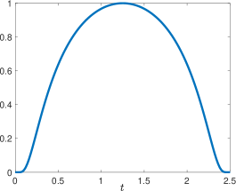
Figure 1. The $C_{0}^{\infty}([0,T])$ function $t\mapsto\chi_{0}(t)$, $t\in[0,T]$ with $T=2.5$.

5.1. Distributed case : initial condition in $H^{k+1}(\Omega)\times H^{k}(\Omega)$ for all $k\in\mathbb{N}$

We consider the simplest situation for which

(Ex1) $$(u_{0},u_{1})=(\sin(\pi x),0)\in H^{k+1}(\Omega)\times H^{k}(\Omega)\quad\forall k\in\mathbb{N}.$$

Compatibility conditions (C1)-(C2) are satisfied for any $j$. Moreover, we use the cut-off functions $\chi_{0}\in C_{0}^{\infty}([0,T])$ and $\chi_{1}\in C_{0}^{\infty}([0,1])$ defined by (43) with $T=2$, $a=0.1$ and $b=0.4$. The null controllability property (A) holds true for this set of data. Since explicit solutions are not available in the distributed case, we define as “exact” solution $(u,\phi)$ the one of (16) from a fine and structured mesh (composed of $409\ 000$ triangles and $205\ 261$ vertices) corresponding to $h\approx 4.41\times 10^{-3}$ and $(u_{h},\phi_{h})\in V_{h}^{p}\times V_{h}^{q}$ with $(p,q)=(3,3)$.

Figure 2-left depicts the evolution of the relative error for the variable $\phi$ with respect to the $L^{2}$-norm

$$\textrm{err}(\phi,\phi_{h},\chi):=\|\chi(\phi-\phi_{h})\|_{L^{2}(M)}/\|\chi\phi\|_{L^{2}(M)}$$

with respect to $h$ for various pairs of $(p,q)$. Table 1 collects the corresponding numerical values. We observe the convergence of the approximation w.r.t. $h$. Moreover, the figure exhibits the influence of the space $V_{h}^{q}$ used for the variable $\phi_{h}$ while the choice of the space $V_{h}^{p}$ for the variable $u_{h}$ has no effect on the approximation. We observe rates close to $0.5$, $2$ and $3$ for $(p,q)=(1,1)$, $(p,q)=(2,2)$ and $(p,q)=(3,3)$ respectively, in agreement with Theorem 2.3. For comparison, Figure 2-right depicts the evolution of the relative error $\textrm{err}(\phi,\phi_{h},\chi)$ for $\chi_{0}(t)=1$ and $\chi_{1}(x)=1_{(a,b)}(x)$, i.e. when no regularization of the control support is introduced. Table 2 collects the corresponding numerical values. The corresponding controlled pair $(u,\phi)$ is a priori only in $C([0,T];H_{0}^{1}(\Omega))\times C([0,T];L^{2}(\Omega))$. Thus, if we still get the convergence with respect to the parameter $h$, we observe that the approximation is not improved beyond the value $q=2$. As before, the choice of the approximation space $V_{h}^{p}$ for $u_{h}$ does not affect the result. The rate is also reduced: for $(p,q)=(2,2)$, the rate is close to $1.5$. This highlights the influence of the cut off functions, including for very smooth initial conditions. Table 3 collects some $L^{2}$ norms of $u_{h}$ and $\phi_{h}$ with respect to $h$ for the pair $(p,q)=(2,2)$: in particular, the relative error $err(u,u_{h},1)$ associated with the controlled solution $u$ is order of $h^{2.5}$ for $h$ small enough.

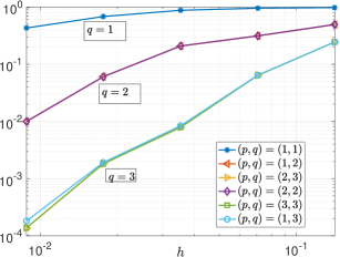
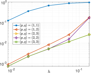
Figure 2. (Ex1); $\|\chi(\phi-\phi_{h})\|_{L^{2}(M)}/\|\chi\phi\|_{L^{2}(M)}$ vs. $h$; Left: $\chi_{0}(t)$ and $\chi_{1}(x)$ given by (43); Right: $\chi_{0}(t)=1$ and $\chi_{1}(x)=1_{(a,b)}(x)$.

$h$	$1.57\times 10^{-1}$	$8.22\times 10^{-2}$	$4.03\times 10^{-2}$	$2.29\times 10^{-2}$	$1.25\times 10^{-2}$
$(p,q)=(1,1)$	$9.81\times 10^{-1}$	$9.58\times 10^{-1}$	$8.81\times 10^{-1}$	$6.83\times 10^{-1}$	$4.31\times 10^{-1}$
$(p,q)=(2,2)$	$4.96\times 10^{-1}$	$3.15\times 10^{-1}$	$2.09\times 10^{-1}$	$6.05\times 10^{-2}$	$1.00\times 10^{-2}$
$(p,q)=(3,3)$	$2.45\times 10^{-1}$	$6.41\times 10^{-2}$	$7.93\times 10^{-3}$	$1.81\times 10^{-3}$	$1.38\times 10^{-4}$

Table 1. (Ex1); $\|\chi(\phi_{h}-\phi)\|_{L^{2}(M)}/\|\chi\phi\|_{L^{2}(M)}$; $\chi$ from (43).

$h$	$1.57\times 10^{-1}$	$8.22\times 10^{-2}$	$4.03\times 10^{-2}$	$2.29\times 10^{-2}$	$1.25\times 10^{-2}$
$(p,q)=(1,1)$	$9.55\times 10^{-1}$	$8.71\times 10^{-1}$	$6.74\times 10^{-1}$	$3.58\times 10^{-1}$	$1.24\times 10^{-1}$
$(p,q)=(2,2)$	$1.71\times 10^{-1}$	$1.57\times 10^{-2}$	$5.20\times 10^{-3}$	$2.24\times 10^{-3}$	$7.47\times 10^{-4}$
$(p,q)=(3,3)$	$2.58\times 10^{-2}$	$1.17\times 10^{-3}$	$5.28\times 10^{-3}$	$2.24\times 10^{-3}$	$7.47\times 10^{-4}$

Table 2. (Ex1); $\|\chi(\phi_{h}-\phi)\|_{L^{2}(\mathcal{M})}/\|\chi\phi\|_{L^{2}(\mathcal{M})}$ ; $\chi_{0}(t)=1;\chi_{1}(x)=1_{(a,b)}(x)$.

$h$	$1.57\times 10^{-1}$	$8.22\times 10^{-2}$	$4.03\times 10^{-2}$	$2.29\times 10^{-2}$	$1.25\times 10^{-2}$
$\textrm{err}(\phi,\phi_{h},1)$	$6.22\times 10^{-1}$	$3.92\times 10^{-1}$	$2.33\times 10^{-1}$	$6.45\times 10^{-2}$	$1.04\times 10^{-2}$
$\textrm{err}(\partial_{x}\phi,\partial_{x}\phi_{h},1)$	$8.11\times 10^{-1}$	$6.84\times 10^{-1}$	$4.85\times 10^{-1}$	$1.64\times 10^{-1}$	$4.57\times 10^{-2}$
$\textrm{err}(u,u_{h},1)$	$4.29\times 10^{-1}$	$1.36\times 10^{-1}$	$5.00\times 10^{-2}$	$1.08\times 10^{-2}$	$1.10\times 10^{-3}$
$\textrm{err}(\phi,\phi_{h},\chi)$	$4.96\times 10^{-1}$	$3.15\times 10^{-1}$	$2.09\times 10^{-1}$	$6.05\times 10^{-2}$	$1.00\times 10^{-2}$

Table 3. (Ex1); $(p,q)=(2,2)$ and $\chi$ from (43).

5.2. Distributed case : initial condition in $H^{1}(\Omega)\times L^{2}(\Omega)$

We consider the initial condition

(Ex2) $$(u_{0},u_{1})=\big{(}4x1_{(0,1/2)}(x)+4(1-x)1_{[1/2,1)}(x),0\big{)}\in H^{1}(\Omega)\times H^{0}(\Omega)$$

for which the compatibility conditions (C1)-(C2) are satisfied for any $j$. If the cut-off functions are introduced, the controlled pair $(u,\phi)$ belongs to $H^{1}(M)\times H^{0}(M)$. Theorem 2.3 does not provide a convergence rate in this case. The strong convergence is however observed: figure 3 displays the relative error wrt $h$ for $(p,q)=(1,1)$, $(p,q)=(2,2)$ and $(p,q)=(3,3)$ with rates close to $1/2$.

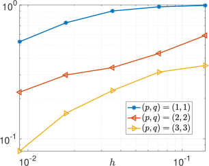
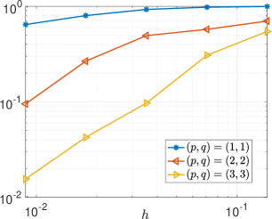
Figure 3. (Ex2) and (Ex2b) ; $\|\chi(\phi-\phi_{h})\|_{L^{2}(M)}/\|\chi\phi\|_{L^{2}(M)}$ vs. $h$; $\chi$ from (43).

$h$	$1.57\times 10^{-1}$	$8.22\times 10^{-2}$	$4.03\times 10^{-2}$	$2.29\times 10^{-2}$	$1.25\times 10^{-2}$
$(p,q)=(1,1)$	$9.89\times 10^{-1}$	$9.66\times 10^{-1}$	$8.99\times 10^{-1}$	$7.34\times 10^{-1}$	$5.30\times 10^{-1}$
$(p,q)=(2,2)$	$5.90\times 10^{-1}$	$4.31\times 10^{-1}$	$3.38\times 10^{-1}$	$2.98\times 10^{-1}$	$2.22\times 10^{-1}$
$(p,q)=(3,3)$	$3.51\times 10^{-1}$	$3.14\times 10^{-1}$	$2.28\times 10^{-1}$	$1.54\times 10^{-1}$	$8.08\times 10^{-2}$

Table 4. (Ex2); $\|\chi(\phi-\phi_{h})\|_{L^{2}(M)}/\|\chi\phi\|_{L^{2}(M)}$; $\chi$ from (43).

A similar behavior is observed with the condition $u_{0}=0$ and $u_{1}=1_{(0.4,0.6)}(x)$ in $L^{2}(\Omega)$ in agreement with Theorem 3

5.3. Distributed case : initial condition in $H^{2}(\Omega)\times H^{1}(\Omega)$

We consider the initial condition

(Ex2b) $$(u_{0},u_{1})=\big{(}\rho(x)\int_{0}^{x}u_{0}^{2}(t)dt,0\big{)}\in H^{2}(\Omega)\times H^{1}(\Omega)$$

where $u_{0}^{2}$ is the initial position defined in (Ex2) and $\rho\in C^{\infty}_{0}(\Omega)$ is introduced in order to preserve the compatibility conditions (C1)-(C2). Figure 3-right displays the convergence of the approximation for $(p,q)=(1,1)$, $(p,q)=(2,2)$ and $(p,q)=(3,3)$. Theorem 2.3 still does not provide a convergence rate in this case. However, with respect to the previous example, smaller relative error with rates close to $1$ are observed for $(p,q)=(2,2)$ and $(p,q)=(3,3)$.

5.4. Boundary case: initial condition in $H^{k+1}(\Omega)\times H^{k}(\Omega)$ for all $k\in\mathbb{N}$

We consider again the simple situation given by the initial condition (Ex1). Compatibility conditions (C1)-(C2) are satisfied for any $j$. In contrast with the distributed case, explicit exact solutions are available in the boundary case when cut-off functions are not introduced. Precisely, the corresponding control of minimal $L^{2}(\Gamma)$ norm with $\Gamma=(0,T=2)\times\{1\}$ is given by $v(t)=\frac{1}{2}\sin(\pi(1-t))=\frac{1}{2}\sin(\pi t)$ leading to $\|v\|_{2}=1/2$. The corresponding controlled solution is given by

(44) $$u(t,x)=\left\{\begin{array}[]{cc}\frac{1}{2}\big{(}u_{0}(x+t)+u_{0}(x-t)\big{)}&x+t\leq 1,\\ \frac{1}{2}u_{0}(x-t),&x+t>1,\,x-t\geq-1,\\ 0,&x-t<-1,\end{array}\right.$$

leading to $\|u\|_{L^{2}(M)}=1/2$. The corresponding adjoint solution is given by $\phi(t,x)=-\frac{1}{2\pi}\sin(\pi t)\sin(\pi x)$ leading to $\|\phi\|_{L^{2}(M)}=\frac{1}{2\sqrt{2}\pi}$ and $\|\partial_{x}\phi\|_{L^{2}(M)}=\frac{1}{2\sqrt{2}}$.

Tables 5 and 6 collects some relative errors w.r.t. $h$ for $(p,q)=(1,2)$ and $(p,q)=(2,3)$ respectively including

$$\textrm{err}(v,u_{h}):=\|v-u_{h}(\cdot,1)\|_{L^{2}(0,T)}/\|v\|_{L^{2}(0,T)},$$

and $\textrm{err}(v,h\chi\partial_{\nu}\phi_{h})$ while Figure 4-left depicts the relative error on the control w.r.t. $h$ for several pairs of $(p,q)$. Since compatibility conditions hold true here, the introduction of the cut off function $\chi\neq 1$ is a priori useless. However, we observe that the term $\partial_{x}\phi(\cdot,1)$ is not well approximated near $t=0$ and $t=T$. This somehow pollutes the approximation $\phi_{h}$ of $\phi$ inside the domain (precisely along the characteristics intersecting the points $(t,x)=(0,1)$ and $(t,x)=(T,1)$ and affects the optimal rate. We observe rate close to $0.75$ for $(p,q)=(1,1)$ and close to $1.5$ otherwise. Imposing in addition $\phi=0$ on the boundary $\partial\Omega$ slightly improves the approximation.

$h$	$1.57\times 10^{-1}$	$8.22\times 10^{-2}$	$4.03\times 10^{-2}$	$2.29\times 10^{-2}$	$1.25\times 10^{-2}$
$\textrm{err}(\phi,\phi_{h},1)$	$7.17\times 10^{-1}$	$1.97\times 10^{-1}$	$4.54\times 10^{-2}$	$1.53\times 10^{-2}$	$4.50\times 10^{-3}$
$\textrm{err}(\partial_{x}\phi,\partial_{x}\phi_{h},1)$	$9.21\times 10^{-1}$	$3.05\times 10^{-1}$	$9.40\times 10^{-2}$	$5.41\times 10^{-2}$	$2.47\times 10^{-2}$
$\textrm{err}(u,u_{h},1)$	$1.88\times 10^{-1}$	$5.73\times 10^{-2}$	$1.92\times 10^{-2}$	$9.29\times 10^{-3}$	$4.09\times 10^{-3}$
$\textrm{err}(v,u_{h})$	$2.16\times 10^{-1}$	$5.83\times 10^{-2}$	$1.94\times 10^{-2}$	$7.21\times 10^{-3}$	$3.10\times 10^{-3}$
$\textrm{err}(v,h\chi\partial_{x}\phi_{h})$	$2.71\times 10^{-1}$	$8.41\times 10^{-2}$	$2.79\times 10^{-2}$	$1.22\times 10^{-2}$	$5.31\times 10^{-3}$

Table 5. (Ex1) - Boundary case - $(p,q)=(1,2)$ - $\chi\equiv 1$.

$h$	$1.57\times 10^{-1}$	$8.22\times 10^{-2}$	$4.03\times 10^{-2}$	$2.29\times 10^{-2}$	$1.25\times 10^{-2}$
$\textrm{err}(\phi,\phi_{h},1)$	$4.09\times 10^{-1}$	$1.15\times 10^{-1}$	$2.82\times 10^{-2}$	$9.29\times 10^{-3}$	$2.81\times 10^{-3}$
$\textrm{err}(\partial_{x}\phi,\partial_{x}\phi_{h},1)$	$6.73\times 10^{-1}$	$2.10\times 10^{-1}$	$6.13\times 10^{-2}$	$2.91\times 10^{-2}$	$1.24\times 10^{-2}$
$\textrm{err}(u,u_{h},1)$	$7.29\times 10^{-2}$	$2.81\times 10^{-2}$	$9.02\times 10^{-3}$	$3.45\times 10^{-3}$	$1.28\times 10^{-3}$
$\textrm{err}(v,u_{h})$	$1.00\times 10^{-1}$	$3.74\times 10^{-2}$	$1.13\times 10^{-2}$	$4.16\times 10^{-3}$	$1.43\times 10^{-3}$
$\textrm{err}(v,h\chi\partial_{x}\phi_{h})$	$1.05\times 10^{-1}$	$3.89\times 10^{-2}$	$1.23\times 10^{-2}$	$4.61\times 10^{-3}$	$1.65\times 10^{-3}$

Table 6. (Ex1) - Boundary case - $(p,q)=(2,3)$ - $\chi\equiv 1$.

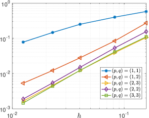
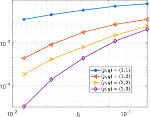
Figure 4. (Ex1) - Boundary case - $\|h\chi\partial_{x}\phi_{h}(1,\cdot)-v\|_{L^{2}(0,T)}/\|v\|_{L^{2}(0,T)}$ vs. $h$ with $\chi=1$ (left) and $\chi=\chi_{0}$ from (43) (right).

With $\chi\neq 1$, the explicit control of minimal $L^{2}(\chi^{1/2},(0,T))$ norm is not available anymore. As for the distributed controllability, we define as “exact” control the one obtained from a fine and uniform mesh (composed of $648\ 000$ triangles and $325\ 261$ vertices) corresponding to $h\approx 3.92\times 10^{-3}$ and $(p,q)=(2,3)$. We take $T$ large enough, precisely $T=2.5$, to ensure the null controllability property of the wave equation. Figure 4-right displays the evolution of $\|h\chi\partial_{x}\phi_{h}(\cdot,1)-v\|_{L^{2}(0,T)}/\|v\|_{L^{2}(0,T)}$ w.r.t. $h$. For $(p,q)=(1,1)$ and $(p,q)=(1,2)$, we observe rates close to $0.5$ and $1.5$ in agreement with (42) of Theorem 4.2 with $\kappa=0$. For $(p,q)=(2,3)$, we observe a rate close to $3$, which is a bit better than the value $2.5$ from (42). Those results also show that the boundary control can be approximated both from the quantity $h\partial_{x}\phi_{h}(\cdot,1)$ obtained from the adjoint dual variable and from the trace $u_{h}(\cdot,1)$ of the primal variable.

5.5. Boundary case: initial condition in $H^{1}(\Omega)\times H^{0}(\Omega)$

We consider the initial data (Ex2). The corresponding control of minimal $L^{2}(\Gamma)$ norm with $\Gamma=(0,T=2)\times\{1\}$ (corresponding to $\chi\equiv 1$)is given by

$$v(t)=2t\,1_{(0,1/2)}(t)+2(1-t)1_{(1/2,3/2)}(t)+2(t-2)\,1_{(3/2,1)}(t).$$

The corresponding controlled solution is explicitly known as follows:

(45) $$u(t,x)=\frac{1}{2}u_{0}(x-t)1_{(t-x\leq 0)}+\frac{1}{2}u_{0}(x+t)1_{(t+x\leq 1)}-\frac{1}{2}u_{0}(t-x)1_{(t-x\geq 0)}1_{(t-x\leq 1)}.$$

The corresponding adjoint solution is given by $\phi(t,x)+\phi(t,1-x)$ where $\phi$ is defined in (47) with the following initial conditions

$$(\phi_{0},\phi_{1})=\big{(}0,-2x\,1_{(0,1/2)}(x)+2(x-1)\,1_{(1/2,1)}(x)\big{)}\in H^{2}(\Omega)\times H^{1}(\Omega).$$

Compatibility conditions are satisfied.

Figure 5-left displays the evolution of $\|\chi\partial_{x}\phi_{h}(1,\cdot)-v\|_{L^{2}(0,T)}/\|v\|_{L^{2}(0,T)}$ w.r.t. $h$ for various pairs of $(p,q)$ and $\chi\equiv 1$. We observe a rate close to $0.75$ for $(p,q)=(1,1)$ and close to $1.5$ otherwise. Remark that a priori $u\in H^{1}(M)$ and $\phi\in H^{2}(M)$ so that the choice $(p,q)=(2,3)$ does not lead to a better rate than the choice $(p,q)=(1,2)$. Moreover, as expected, the introduction of the cut off $\chi\neq 1$ does not improve here the rate of convergence: see Figure 5-right where similar rates are observed.

$h$	$1.57\times 10^{-1}$	$8.22\times 10^{-2}$	$4.03\times 10^{-2}$	$2.29\times 10^{-2}$	$1.25\times 10^{-2}$
$\textrm{err}(\phi,\phi_{h},1)$	$7.83\times 10^{-1}$	$2.53\times 10^{-1}$	$5.82\times 10^{-2}$	$1.97\times 10^{-2}$	$5.64\times 10^{-3}$
$\textrm{err}(\partial_{x}\phi,\partial_{x}\phi_{h},1)$	$1.12\times 10^{0}$	$5.03\times 10^{-1}$	$2.02\times 10^{-1}$	$1.12\times 10^{-1}$	$5.04\times 10^{-2}$
$\textrm{err}(u,u_{h},1)$	$1.91\times 10^{-1}$	$4.94\times 10^{-2}$	$2.42\times 10^{-2}$	$1.17\times 10^{-2}$	$5.04\times 10^{-3}$
$\textrm{err}(v,u_{h})$	$2.20\times 10^{-1}$	$6.48\times 10^{-2}$	$2.87\times 10^{-2}$	$1.16\times 10^{-2}$	$4.95\times 10^{-3}$
$\textrm{err}(v,h\chi\partial_{x}\phi_{h})$	$2.49\times 10^{-1}$	$6.41\times 10^{-2}$	$2.97\times 10^{-2}$	$1.40\times 10^{-2}$	$6.06\times 10^{-3}$

Table 7. (Ex2) - Boundary case - $(p,q)=(1,2)$; $\chi\equiv 1$

$h$	$1.57\times 10^{-1}$	$8.22\times 10^{-2}$	$4.03\times 10^{-2}$	$2.29\times 10^{-2}$	$1.25\times 10^{-2}$
$\textrm{err}(\phi,\phi_{h},1)$	$4.90\times 10^{-1}$	$1.35\times 10^{-1}$	$3.28\times 10^{-2}$	$1.07\times 10^{-2}$	$3.41\times 10^{-3}$
$\textrm{err}(\partial_{x}\phi,\partial_{x}\phi_{h},1)$	$9.79\times 10^{-1}$	$3.75\times 10^{-1}$	$1.35\times 10^{-1}$	$6.76\times 10^{-2}$	$3.21\times 10^{-2}$
$\textrm{err}(u,u_{h},1)$	$6.70\times 10^{-2}$	$2.60\times 10^{-2}$	$9.34\times 10^{-3}$	$3.78\times 10^{-3}$	$1.44\times 10^{-3}$
$\textrm{err}(v,u_{h})$	$8.61\times 10^{-2}$	$3.25\times 10^{-2}$	$1.10\times 10^{-2}$	$4.19\times 10^{-3}$	$1.59\times 10^{-3}$
$\textrm{err}(v,h\chi\partial_{x}\phi_{h})$	$8.57\times 10^{-2}$	$3.23\times 10^{-2}$	$1.10\times 10^{-2}$	$4.45\times 10^{-3}$	$1.71\times 10^{-3}$

Table 8. (Ex2) - Boundary case - $(p,q)=(2,3)$; $\chi\equiv 1$

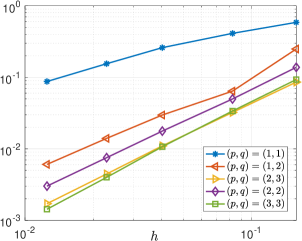
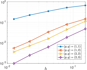
Figure 5. (Ex2) - Boundary case - $\|h\partial_{x}\chi\phi_{h}(1,\cdot)-v\|_{L^{2}(0,T)}/\|v\|_{L^{2}(0,T)}$ vs. $h$ with $\chi=1$ (left) and $\chi=\chi_{0}$ from (43) (right).

5.6. Boundary case: initial condition in $H^{0}(\Omega)\times H^{-1}(\Omega)$

We consider the following stiff situation given by

(Ex3) $$(u_{0},u_{1})=(4x1_{(0,1/2)}(x),0)\in H^{0}(\Omega)\times H^{-1}(\Omega).$$

and extensively discussed in [15, 44] and $T=2$. The corresponding control of minimal $L^{2}((0,T)\times\{1\})$ norm is given by $v(t)=2(1-t)1_{(1/2,3/2)}(t)$ leading to $\|v\|_{L^{2}(0,T)}=1/\sqrt{3}$. The corresponding controlled solution is explicitly known as follows:

(46) $$u(t,x)=\left\{\begin{array}[]{cc}4x&0\leq x+t<\frac{1}{2},\\ 2(x-t)&-\frac{1}{2}<t-x<\frac{1}{2},\quad x+t\geq\frac{1}{2},\\ 0&else,\end{array}\right.$$

leading to $\|u\|_{L^{2}(M)}=1/\sqrt{3}$. The corresponding initial conditions of the adjoint solution is $(\phi_{0},\phi_{1})=(0,-2x\,1_{(0,1/2)}(x))\in H^{1}(\Omega)\times H^{0}(\Omega)$ leading to

(47) $$\phi(t,x)=\left\{\begin{array}[]{cc}-2xt&0\leq x+t<\frac{1}{2},\quad x\geq 0,t\geq 0,\\ \frac{(x-t)^{2}}{2}-\frac{1}{8}&\frac{1}{2}\leq x+t<\frac{3}{2},\quad-\frac{1}{2}<x-t<\frac{1}{2},\\ 2(x-1)(1-t)&\frac{3}{2}\leq x+t,\quad-\frac{1}{2}<x-t,\\ -\frac{(x+t-2)^{2}}{2}+\frac{1}{8}&\frac{3}{2}<x+t<\frac{5}{2},\quad-\frac{3}{2}<x-t\leq-\frac{1}{2},\\ 2x(2-t)&x-t\leq-\frac{3}{2},\end{array}\right.$$

leading to $\|\phi\|_{L^{2}(M)}\approx 9.86\times 10^{2}$ and $\|\partial_{x}\phi\|_{L^{2}(M)}\approx 4.08\times 10^{-1}$. In particular, we check that $\partial_{x}\phi(t,x)_{|x=1}=2(1-t)\,1_{(1/2,3/2)}(t)=v(t).$ Both $u$ and $\phi$ develop singularities (where $u$ and $\nabla\phi$ are discontinuous).

Figure 6 depicts the evolution of $\|h\chi\partial_{x}\phi_{h}(\cdot,1)-v\|_{L^{2}(0,T)}/\|v\|_{L^{2}(0,T)}$ w.r.t. $h$ with $\chi\equiv 1$. We observe a rate close to $0.5$.

Let us also emphasize that the space-time discretization formulation is very well appropriated for mesh adaptivity. Using the $V_{h}^{1}\times V_{h}^{2}$ approximation, Figure 7-left (resp. right) depicts the mesh obtained after seven adaptative refinements based on the local values of gradient of the variable $\phi_{h}$ (resp. $u_{h}$). Starting with a coarse mesh composed of $288$ triangles and $166$ vertices, the final mesh on the right is composed with $13068$ triangles and $6700$ vertices and leads to a relative error $\textrm{err}(v,u_{h})$ of the order of $10^{-3}$. The final mesh follows the singularities of the controlled solution starting at the point $(0,1)$ of discontinuity of $u_{0}$.

$h$	$1.57\times 10^{-1}$	$8.22\times 10^{-2}$	$4.03\times 10^{-2}$	$2.29\times 10^{-2}$	$1.25\times 10^{-2}$
$\textrm{err}(\phi,\phi_{h},1)$	$6.38\times 10^{-1}$	$4.35\times 10^{-1}$	$2.85\times 10^{-1}$	$1.84\times 10^{-1}$	$1.05\times 10^{-1}$
$\textrm{err}(\partial_{x}\phi,\partial_{x}\phi_{h},1)$	$8.38\times 10^{-1}$	$6.23\times 10^{-1}$	$4.85\times 10^{-1}$	$3.97\times 10^{-1}$	$3.17\times 10^{-1}$
$\textrm{err}(u,u_{h},1)$	$5.78\times 10^{-1}$	$4.40\times 10^{-1}$	$3.59\times 10^{-1}$	$2.93\times 10^{-1}$	$2.27\times 10^{-1}$
$\textrm{err}(v,u_{h})$	$7.67\times 10^{-1}$	$5.69\times 10^{-1}$	$5.04\times 10^{-1}$	$4.05\times 10^{-1}$	$3.15\times 10^{-1}$
$\textrm{err}(v,h\chi\partial_{x}\phi_{h})$	$8.41\times 10^{-1}$	$6.47\times 10^{-1}$	$5.08\times 10^{-1}$	$4.09\times 10^{-1}$	$3.16\times 10^{-1}$

Table 9. (Ex3); $(p,q)=(1,1)$ - $\chi\equiv 1$ - Boundary case

$h$	$1.57\times 10^{-1}$	$8.22\times 10^{-2}$	$4.03\times 10^{-2}$	$2.29\times 10^{-2}$	$1.25\times 10^{-2}$
$\textrm{err}(\phi,\phi_{h},1)$	$1.62\times 10^{0}$	$6.33\times 10^{-1}$	$2.72\times 10^{-1}$	$1.45\times 10^{-1}$	$7.36\times 10^{-2}$
$\textrm{err}(\partial_{x}\phi,\partial_{x}\phi_{h},1)$	$2.33\times 10^{0}$	$1.52\times 10^{0}$	$1.22\times 10^{0}$	$1.08\times 10^{0}$	$1.05\times 10^{0}$
$\textrm{err}(u,u_{h},1)$	$3.93\times 10^{-1}$	$3.00\times 10^{-1}$	$2.27\times 10^{-1}$	$1.74\times 10^{-1}$	$1.30\times 10^{-1}$
$\textrm{err}(v,u_{h})$	$5.03\times 10^{-1}$	$3.43\times 10^{-1}$	$2.41\times 10^{-1}$	$1.89\times 10^{-1}$	$1.48\times 10^{-1}$
$\textrm{err}(v,h\chi\partial_{x}\phi_{h})$	$4.73\times 10^{-1}$	$3.41\times 10^{-1}$	$2.64\times 10^{-1}$	$2.08\times 10^{-1}$	$1.60\times 10^{-1}$

Table 10. (Ex3); $(p,q)=(1,2)$ - $\chi\equiv 1$ - Boundary case

$h$	$1.57\times 10^{-1}$	$8.22\times 10^{-2}$	$4.03\times 10^{-2}$	$2.29\times 10^{-2}$	$1.25\times 10^{-2}$
$\textrm{err}(\phi,\phi_{h},1)$	$1.25\times 10^{0}$	$5.01\times 10^{-1}$	$2.02\times 10^{-1}$	$9.58\times 10^{-2}$	$4.52\times 10^{-2}$
$\textrm{err}(\partial_{x}\phi,\partial_{x}\phi_{h},1)$	$3.44\times 10^{0}$	$2.34\times 10^{0}$	$1.88\times 10^{0}$	$1.57\times 10^{0}$	$1.45\times 10^{0}$
$\textrm{err}(u,u_{h},1)$	$3.12\times 10^{-1}$	$2.22\times 10^{-1}$	$1.60\times 10^{-1}$	$1.24\times 10^{-1}$	$9.01\times 10^{-2}$
$\textrm{err}(v,u_{h})$	$3.52\times 10^{-1}$	$2.36\times 10^{-1}$	$1.71\times 10^{-1}$	$1.30\times 10^{-1}$	$9.64\times 10^{-2}$
$\textrm{err}(v,h\chi\partial_{x}\phi_{h})$	$3.40\times 10^{-1}$	$2.36\times 10^{-1}$	$1.66\times 10^{-1}$	$1.37\times 10^{-1}$	$9.56\times 10^{-2}$

Table 11. (Ex3); $(p,q)=(2,3)$ - $\chi\equiv 1$ - Boundary case

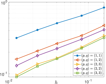
Figure 6. (Ex3); $\|h\chi\partial_{x}\phi_{h}(\cdot,1)-v\|_{L^{2}(0,T)}/\|v\|_{L^{2}(0,T)}$ w.r.t. $h$ (rate $\approx 0.5$).

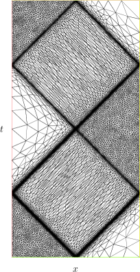
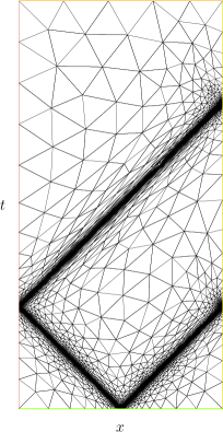
Figure 7. (Ex3); Locally refine space-time meshes with respect to $\phi_{h}$ (left) and $u_{h}$ (right). $(p,q)=(1,2)$

5.7. Boundary case: the wave equation with a potential

To end these numerical illustrations, we report some results for the wave equation with non vanishing potential $V$, see (31). Non zero potentials notably appear from linearization of nonlinear wave equations of the form $\Box u+f(u)=\chi v$ (see [45]). Actually, we want to emphasize that this spacetime approach, based on the resolution of the optimal condition associated with the control of minimal $L^{2}$ norm is very relevant for potential with the “bad” sign for which $V(t,x)u(t,x)<0$. Indeed, in this case, the usual “à la Glowinski” strategy developed in [26] is numerically inefficient and requires adaptations, since the uncontrolled solution (used to initialize the conjugate algorithm) grows exponentially in time, leading to numerical instabilities and overflow. Recall that the observability constant behaves like $e^{C(T,\omega)\|A\|^{2}_{L^{\infty}(0,T;L^{n}(\Omega))}}$ (see [49]) and appears notably in the constant in the a priori estimate (42). We consider the initial condition (Ex1), $T=2.5$ and constant negative potentials $V(t,x)=V<0$. Table 12 collects the relative error on the approximation of the boundary control with respect to $h$ for several negatives values of $V$. In particular, for $V=-40$, the $L^{\infty}$ norm of the corresponding uncontrolled solution is of order $10^{5}$. We approximate $u$ and $\phi$ in $V_{h}^{1}$ and $V_{h}^{2}$ respectively and observe a rate close to $1.5$. The value of $V$ only affects the constant. We refer to [41] for a semi-discrete (in space) approximation of exact boundary controls for a semi-discretized wave equation with potential, including experiments for small and potentials with good sign.

$h$	$1.6\times 10^{-1}$	$8\times 10^{-2}$	$4\times 10^{-2}$	$2\times 10^{-2}$	$1\times 10^{-2}$
$V=-10$	$7.11\times 10^{-1}$	$2.43\times 10^{-1}$	$6.91\times 10^{-2}$	$2.48\times 10^{-2}$	$7.97\times 10^{-3}$
$V=-20$	$7.06\times 10^{-1}$	$2.81\times 10^{-1}$	$1.57\times 10^{-1}$	$6.13\times 10^{-2}$	$1.65\times 10^{-2}$
$V=-30$	$9.54\times 10^{-1}$	$6.91\times 10^{-1}$	$2.07\times 10^{-1}$	$7.21\times 10^{-2}$	$2.27\times 10^{-2}$
$V=-40$	$1.01\times 10^{-1}$	$9.44\times 10^{-1}$	$5.05\times 10^{-1}$	$1.13\times 10^{-1}$	$3.18\times 10^{-2}$

Table 12. (Ex1) - Boundary case - $(p,q)=(1,2)$ - $\chi$ from (43); $\|h\chi\partial_{x}\phi_{h}(\cdot,1)-v\|_{L^{2}(0,T)}/\|v\|_{L^{2}(0,T)}$ w.r.t. $h$ and $V\in\{-10,-20,-30,-40\}$.

6. Conclusion

We have introduced and analyzed a spacetime finite element approximation of a controllability problem for the wave equation. Based on a non conformal $H^{1}$-approximation, the analysis yields error estimates for the control in the natural $L^{2}$ -norm of order $h^{q}$ (resp. $h^{q-\frac{1}{2}}$) where $q$ is the degree of the polynomials used to describe the adjoint variable in the distributed (resp. boundary) case. The numerical experiments performed for initial data with various regularity exhibits the efficiency method. The convergence is also observed for initial data with minimal regularity.

We emphasize that spacetime formulations are easier to implement than time-marching methods, since in particular, there is no kind of CFL condition between the time and space discretization parameters. Moreover, as shown in the numerical section, they are well-suited for mesh adaptivity (as initially discussed in [30]).

Similarly to the formulation proposed in [13, 15], the present formulation follows the “control then discretize” approach. However, contrary to [13, 15], the $H^{1}$-formulation of the present work does not require the introduction of sophisticated finite element spaces. On the other hand, the formulation requires additional stabilized terms which are function of the jump of the gradient across the boundary of each element. The analysis is then inspired from [10] and also from [8] where an analogous spacetime formulation for a data assimilation is considered.

The implementation of the stabilized terms is not straightforward, in particular, in higher dimension, and is usually not available in finite element softwares. A possible way to circumvent the introduction of the gradient jump terms is to consider non-conforming approximation of the Crouzeix-Raviart type as in [7]. A penalty is then needed on the solution jump instead to control the $H^{1}$-conformity error. Another possible way, following [43] devoted to the boundary case, could be to consider the controllability problem associated to a first order reformulation of the wave equation:

(48) $$\begin{cases}v_{t}-div\,\mathbf{p}=0,\\ \mathbf{p}_{t}-\nabla v=0.\end{cases}$$

with $v:=u_{t}$ and $\mathbf{p}:=\nabla u$. A $H^{1}$ conformal stabilized approximation is employed in [43] leading to promising numerical experiments in the one dimensional case. A rigorous numerical analysis however remains to be done.

Appendix A Continuum estimates

Proposition (Energy estimate).

There holds

(49) $$\lVert u\rVert_{L^{\infty}(0,T;L^{2}(\Omega))}+\lVert\partial_{t}u\rVert_{L^{2}(0,T;H^{-1}(\Omega))}+\lVert\partial_{\nu}u\rVert_{H^{-1}((0,T)\times\partial\Omega)}$$

$$\quad\lesssim\lVert u|_{t=0}\rVert_{L^{2}(\Omega)}+\lVert\partial_{t}u|_{t=0}\rVert_{H^{-1}(\Omega)}+\lVert u\rVert_{L^{2}((0,T)\times\partial\Omega)}+\lVert\Box u\rVert_{H^{-1}((0,T)\times\Omega)}.$$

Proof.

The estimate

(50) $$\lVert u\rVert_{L^{\infty}(0,T;L^{2}(\Omega))}+\lVert\partial_{t}u\rVert_{L^{\infty}(0,T;H^{-1}(\Omega))}+\lVert\partial_{\nu}u\rVert_{H^{-1}((0,T)\times\partial\Omega)}$$

$$\quad\lesssim\lVert u|_{t=0}\rVert_{L^{2}(\Omega)}+\lVert\partial_{t}u|_{t=0}\rVert_{H^{-1}(\Omega)}+\lVert u\rVert_{L^{2}((0,T)\times\partial\Omega)}+\lVert\Box u\rVert_{L^{1}(0,T;H^{-1}(\Omega))}$$

follows from [34, Theorem 2.3], see also Remark 2.2 there. Thus it is enough to consider the equation

(51) $$\begin{cases}\Box u=f,\\ u|_{x\in\partial\Omega}=0,\\ u|_{t<0}=0,\end{cases}$$

and show that its solution satisfies

$$\lVert u\rVert_{L^{\infty}(0,T;L^{2}(\Omega))}+\lVert\partial_{t}u\rVert_{L^{2}(0,T;H^{-1}(\Omega))}+\lVert\partial_{\nu}u\rVert_{H^{-1}((0,T)\times\partial\Omega)}\lesssim\lVert f\rVert_{H^{-1}((0,T)\times\Omega)}.$$

Let us use the shorthand notations $M=(0,T)\times\Omega$ and $(t,x)=(x^{0},\dots,x^{n})$. We recall that for any $f\in H^{-1}(M)$ there are $f_{j}\in L^{2}(M)$, $j=-1,0,\dots,n$, such that

(52) $$f=f_{-1}+\sum_{j=0}^{n}\partial_{x^{j}}f_{j},$$

and that

$$\lVert f\rVert_{H^{-1}(M)}^{2}=\inf\sum_{j=-1}^{n}\lVert f_{j}\rVert_{L^{2}(M)}^{2},$$

where the infimum is taken over all $f_{j}\in L^{2}(M)$ satisfying (52), see e.g. [22, Theorem 1, p. 299]. Thus it is enough to show that

$$\lVert u\rVert_{L^{\infty}(0,T;L^{2}(\Omega))}+\lVert\partial_{t}u\rVert_{L^{2}(0,T;L^{2}(\Omega))}+\lVert\partial_{\nu}u\rVert_{H^{-1}((0,T)\times\partial\Omega)}\lesssim\lVert f_{j}\rVert_{L^{2}((0,T)\times\Omega)},$$

where $u$ satisfies (51) with $f$ replaced by $\partial_{x^{j}}f_{j}$ when $j\geq 0$ and by $f_{-1}$ when $j=-1$. The cases $j=-1$ and $j>0$ are contained in (50).

Let us consider the case $j=0$. We denote by $v$ the solution of (51) with $f=f_{0}$. Then $u=\partial_{t}v$ and it follows from [34, Theorem 2.1] that

$$\lVert u\rVert_{L^{\infty}(0,T;L^{2}(\Omega))}+\lVert\partial_{\nu}u\rVert_{H^{-1}((0,T)\times\partial\Omega)} \lesssim\lVert\partial_{t}v\rVert_{L^{\infty}(0,T;L^{2}(\Omega))}+\lVert\partial_{\nu}v\rVert_{L^{2}((0,T)\times\partial\Omega)}$$

$$\lesssim\lVert f_{0}\rVert_{L^{2}((0,T)\times\Omega)}.$$

Moreover,

$$\lVert\partial_{t}u\rVert_{L^{2}(0,T;H^{-1}(\Omega))}=\lVert\partial_{t}^{2}v\rVert_{L^{2}(0,T;H^{-1}(\Omega))}\leq\lVert\Delta v\rVert_{L^{2}(0,T;H^{-1}(\Omega))}+\lVert f_{0}\rVert_{L^{2}(0,T;H^{-1}(\Omega))},$$

and using [34, Theorem 2.1] again,

$$\lVert\Delta v\rVert_{L^{2}(0,T;H^{-1}(\Omega))}\lesssim\lVert v\rVert_{L^{2}(0,T;H^{1}(\Omega))}\lesssim\lVert f_{0}\rVert_{L^{2}((0,T)\times\Omega)}.$$

∎

It is not possible to improve the $L^{2}(0,T;H^{-1}(\Omega))$ norm of $\partial_{t}u$ on the left-hand side of (49) to its $L^{\infty}(0,T;H^{-1}(\Omega))$ norm.

Proof.

To get a contradiction, we suppose that

$$\lVert\partial_{t}u\rVert_{L^{\infty}(0,T;H^{-1}(\Omega))}\lesssim\lVert\Box u\rVert_{H^{-1}((0,T)\times\Omega)}$$

for solutions $u$ of (51). Let $f\in L^{2}(0,T)$, and denote by $u$ and $v$ the solutions of (51) with sources $\partial_{t}f$ and $f$, respectively. Then $u=\partial_{t}v$ and

$$f=\partial_{t}^{2}v-\Delta v=\partial_{t}u-\Delta v\in L^{\infty}(0,T;H^{-1}(\Omega)).$$

But this implies that $f\in L^{\infty}(0,T)$. As $f\in L^{2}(0,T)$ was arbitrary, we get the contradiction $L^{2}(0,T)\subset L^{\infty}(0,T)$. ∎

If $\Box u=0$ and $u|_{x\in\partial\Omega}=0$ then the norm on the left-hand side of (49) controls the $L^{\infty}(0,T;H^{-1}(\Omega))$ norm of $\partial_{t}u$. In fact, we have:

Suppose that $u\in L^{2}((0,T)\times\Omega)$ satisfies $\Box u=0$ and $u|_{x\in\partial\Omega}=0$. Then

$$\lVert u\rVert_{L^{\infty}(0,T;L^{2}(\Omega))}+\lVert\partial_{t}u\rVert_{L^{\infty}(0,T;H^{-1}(\Omega))}+\lVert\partial_{\nu}u\rVert_{H^{-1}((0,T)\times\partial\Omega)}\lesssim\lVert u\rVert_{L^{2}((0,T)\times\Omega)}.$$

Moreover, $u\in C(0,T;L^{2}(\Omega))\cap C^{1}(0,T;H^{-1}(\Omega))$.

Proof.

Let $\chi\in C^{\infty}(\mathbb{R})$ satisfy $\chi(t)=0$ near $t=T$ and $\chi(t)=1$ for $t\in(0,T/2)$. Applying Proposition A to $\chi u$ backwards in time, we obtain

$$\lVert u\rVert_{L^{\infty}(0,T/2;L^{2}(\Omega))}+\lVert\partial_{t}u\rVert_{L^{2}(0,T/2;H^{-1}(\Omega))}\lesssim\lVert[\Box,\chi]u\rVert_{H^{1}((0,T)\times\Omega)}\lesssim\lVert u\rVert_{L^{2}((0,T)\times\Omega)}.$$

Applying (50) backwards in time on the interval $(0,s)$ where $s<T/2$, we get

$$\lVert\partial_{t}u|_{t=0}\rVert_{H^{-1}(\Omega)}^{2}\lesssim\lVert u|_{t=s}\rVert_{L^{2}(\Omega)}^{2}+\lVert\partial_{t}u|_{t=s}\rVert_{H^{-1}(\Omega)}^{2}.$$

Integration in $s$ gives

$$\lVert\partial_{t}u|_{t=0}\rVert_{H^{-1}(\Omega)}^{2}\lesssim \lVert u\rVert_{L^{2}(0,T/2;L^{2}(\Omega))}^{2}+\lVert\partial_{t}u\rVert_{L^{2}(0,T/2;H^{-1}(\Omega))}^{2}.$$

We conclude that

$$\lVert u|_{t=0}\rVert_{L^{2}(\Omega)}+\lVert\partial_{t}u|_{t=0}\rVert_{H^{-1}(\Omega)}\lesssim\lVert u\rVert_{L^{2}((0,T)\times\Omega)}.$$

The claimed estimate follows from (50).

Let us now turn the claimed continuity. Let $\epsilon>0$ and $u_{j}$ be a mollification in time that satisfies $u_{j}\to u$ in $L^{2}((\epsilon,T-\epsilon)\times\Omega)$. Then $u_{j}$ converges in

$$C(\epsilon,T-\epsilon;L^{2}(\Omega))\cap C^{1}(\epsilon,T-\epsilon;H^{-1}(\Omega))$$

and thus $u$ is in this space. In particular, $u|_{t=T/2}$ and $\partial_{t}u|_{t=T/2}$ are well-defined. Solving the initial value problem starting from these gives the desired conclusion. ∎

[Distributed observability estimate] Let $T>0$ and let an open set $\omega\subset\Omega$ satisfy the geometric control condition. Then

$$\lVert\phi|_{t=0}\rVert_{L^{2}(\Omega)}+\lVert\partial_{t}\phi|_{t=0}\rVert_{H^{-1}(\Omega)}\lesssim\lVert\phi\rVert_{L^{2}((0,T)\times\omega)}+\lVert\phi\rVert_{L^{2}((0,T)\times\partial\Omega)}+\lVert\Box\phi\rVert_{H^{-1}((0,T)\times\Omega)}.$$

Proof.

It is classical that

(53) $$\lVert\psi|_{t=0}\rVert_{L^{2}(\Omega)}+\lVert\partial_{t}\psi|_{t=0}\rVert_{H^{-1}(\Omega)}\lesssim\lVert\psi\rVert_{L^{2}((0,T)\times\omega)}$$

when

$$\begin{cases}\Box\psi=0,\\ \psi|_{x\in\partial\Omega}=0,\end{cases}$$

see e.g. [35]. Let $u$ solve

$$\begin{cases}\Box u=\Box\phi,\\ u|_{x\in\partial\Omega}=\phi|_{x\in\partial\Omega},\\ u|_{t=0}=0,\ \partial_{t}u|_{t=0}=0,\end{cases}$$

and define $\psi=\phi-u$. Then using (53) and (49),

$$\lVert\phi|_{t=0}\rVert_{L^{2}(\Omega)}+\lVert\partial_{t}\phi|_{t=0}\rVert_{H^{-1}(\Omega)}=\lVert\psi|_{t=0}\rVert_{L^{2}(\Omega)}+\lVert\partial_{t}\psi|_{t=0}\rVert_{H^{-1}(\Omega)}$$

$$\quad\lesssim\lVert\psi\rVert_{L^{2}((0,T)\times\omega)}\leq\lVert\phi\rVert_{L^{2}((0,T)\times\omega)}+\lVert u\rVert_{L^{2}((0,T)\times\omega)}$$

$$\quad\lesssim\lVert\phi\rVert_{L^{2}((0,T)\times\omega)}+\lVert\phi\rVert_{L^{2}((0,T)\times\partial\Omega)}+\lVert\Box\phi\rVert_{H^{-1}((0,T)\times\Omega)}.$$

∎

By applying Theorem A to the function $(t,x)\mapsto\phi(T-t,x)$ we obtain the following variant

$$\lVert\phi|_{t=T}\rVert_{L^{2}(\Omega)}+\lVert\partial_{t}\phi|_{t=T}\rVert_{H^{-1}(\Omega)}\lesssim\lVert\phi\rVert_{L^{2}((0,T)\times\omega)}+\lVert\phi\rVert_{L^{2}((0,T)\times\partial\Omega)}+\lVert\Box\phi\rVert_{H^{-1}((0,T)\times\Omega)},$$

and by combining Proposition A and Theorem A, we get

$$\lVert\phi\rVert_{L^{\infty}(0,T;L^{2}(\Omega))}+\lVert\partial_{t}\phi\rVert_{L^{2}(0,T;H^{-1}(\Omega))}$$

$$\quad\lesssim\lVert\phi\rVert_{L^{2}((0,T)\times\omega)}+\lVert\phi\rVert_{L^{2}((0,T)\times\partial\Omega)}+\lVert\Box\phi\rVert_{H^{-1}((0,T)\times\Omega)},$$

assuming that $T>0$ and $\omega\subset\Omega$ satisfy the geometric control condition.

[Boundary observability estimate] Let $T>0$ and let an open set $\omega\subset\partial\Omega$ satisfy the geometric control condition. Let $V\in C^{\infty}(\Omega)$ and define $P$ by (31). Then

(54) $$\lVert\phi|_{t=0}\rVert_{L^{2}(\Omega)}+\lVert\partial_{t}\phi|_{t=0}\rVert_{H^{-1}(\Omega)}$$

$$\quad\lesssim\lVert\partial_{\nu}\phi\rVert_{H^{-1}((0,T)\times\omega)}+\lVert\phi\rVert_{L^{2}((0,T)\times\partial\Omega)}+\lVert P\phi\rVert_{H^{-1}((0,T)\times\Omega)}.$$

Proof.

It is well-known that

(55) $$\lVert\psi|_{t=0}\rVert_{L^{2}(\Omega)}+\lVert\partial_{t}\psi|_{t=0}\rVert_{H^{-1}(\Omega)}\lesssim\lVert\partial_{\nu}\psi\rVert_{H^{-1}((0,T)\times\omega)}$$

for solutions $\psi$ of

(56) $$\begin{cases}P\psi=0,\\ \psi|_{x\in\partial\Omega}=0.\end{cases}$$

However, we did not find this exact formulation in the literature, and give a short proof for the convenience of the reader. noline, size=]To Arnaud: do you know a good ref? It follows from (3.11) of the classical paper [4] that

(57) $$\lVert\psi\rVert_{L^{2}((0,T)\times\Omega)}\lesssim\lVert\partial_{\nu}\psi\rVert_{H^{-1}((0,T)\times\omega)},$$

since the space of invisible solutions is empty in our case due to unique continuation. Let $\tau\in C^{\infty}(\mathbb{R})$ satisfy $\tau(t)=1$ near $t=0$ and $\tau(t)=0$ near $t=T$. Writing $u=\tau\psi$ and $f=\partial_{t}\tau\,\partial_{t}\psi+\partial_{t}^{2}\tau\,\psi$, there holds

$$\begin{cases}Pu=f,\\ u|_{x\in\partial\Omega}=0,\\ u|_{t>T}=0.\end{cases}$$

As $\psi\in L^{2}((0,T)\times\Omega)$, we have using $P\psi=0$,

$$\lVert\partial_{t}^{2}\psi\rVert_{L^{2}(0,T;H^{-2}(\Omega))}=\lVert\Delta\psi\rVert_{L^{2}(0,T;H^{-2}(\Omega))}+\lVert V\psi\rVert_{L^{2}(0,T;H^{-2}(\Omega))}\lesssim\lVert\psi\rVert_{L^{2}((0,T)\times\Omega)}.$$

Now interpolation, see e.g. [37, Theorems 2.3 and 12.2], gives

$$\lVert\partial_{t}\psi\rVert_{L^{2}(0,T;H^{-1}(\Omega))}\lesssim\lVert\psi\rVert_{L^{2}(0,T;L^{2}(\Omega))}.$$

Hence also

$$\lVert f\rVert_{L^{2}(0,T;H^{-1}(\Omega))}\lesssim\lVert\psi\rVert_{L^{2}(0,T;L^{2}(\Omega))},$$

and (50), or rather its analogue backward in time, gives

$$\lVert u|_{t=0}\rVert_{L^{2}(\Omega)}+\lVert\partial_{t}u|_{t=0}\rVert_{H^{-1}(\Omega)}\lesssim\lVert\psi\rVert_{L^{2}(0,T;L^{2}(\Omega))}.$$

But the state of $u$ at $t=0$ coincides with that of $\psi$, and (55) follows from the above estimate and (57).

Will now show (54). Let $v$ be the solution of

$$\begin{cases}Pv=P\phi\\ v|_{x\in\partial\Omega}=\phi|_{x\in\partial\Omega}\\ v|_{t<0}=0.\end{cases}$$

Then $\psi=\phi-v$ solves (56), and (55) and (49) imply

$$\lVert\phi|_{t=0}\rVert_{L^{2}(\Omega)}+\lVert\partial_{t}\phi|_{t=0}\rVert_{H^{-1}(\Omega)}=\lVert\psi|_{t=0}\rVert_{L^{2}(\Omega)}+\lVert\partial_{t}\psi|_{t=0}\rVert_{H^{-1}(\Omega)}$$

$$\quad\lesssim\lVert\partial_{\nu}\phi\rVert_{H^{-1}((0,T)\times\omega)}+\lVert\partial_{\nu}v\rVert_{H^{-1}((0,T)\times\omega)}$$

$$\quad\lesssim\lVert\partial_{\nu}\phi\rVert_{H^{-1}((0,T)\times\omega)}+\lVert\phi\rVert_{L^{2}((0,T)\times\partial\Omega)}+\lVert P\phi\rVert_{H^{-1}((0,T)\times\Omega)}.$$

∎

The analogue of Remark A holds also in the case of boundary observations. We need also the following classical result.

[Partial hypoellipticity] Let $I\subset(0,T)$ be a compact interval. Suppose that $s\in\mathbb{R}$ and $j\in\mathbb{N}$ satisfy $s+1/2>j$. Then

$$\lVert\partial_{\nu}^{j}u\rVert_{H^{s-j-\frac{3}{2}}(I\times\partial\Omega)}\lesssim\lVert u\rVert_{H^{s}(M)}+\lVert\Box u\rVert_{H^{s-1}(M)}.$$

Proof.

We define a norm $\lVert u\rVert_{X}$ by the right-hand side of the claimed inequality, and set $X=\{u\in H^{s}(M):\lVert u\rVert_{X}<\infty\}$. It follows from the closed graph theorem that $X$ is a Banach space. In normal coordinates of $\mathbb{R}\times\partial\Omega$, there holds

$$\Box=\partial_{\nu}^{2}+A,$$

where $A$ is a differential operator in the tangential directions to $\mathbb{R}\times\partial\Omega$, with coefficients depending on all the variables, see e.g. [29, Corollary C.5.3].

We will use the spaces $\bar{H}_{(m,s)}(I\times\Omega)$, defined on p. 478 of [29], in the boundary normal coordinates, and use the shorthand notation $H_{(m,s)}$ for them. Here $m$ measures Sobolev smoothness in all the variables and $s$ additional smoothness in the tangential variables. However, $s$ can be also negative, corresponding to a loss of smoothness in tangential directions.

Let $u\in X$. It follows from [29, Theorem B.2.9] that $u\in H_{(m,r)}$ when $m+r\leq s-1$ and $m\leq s+1$. In particular, $u\in H_{(s+1,-2)}$ and the closed graph theorem implies

$$\lVert u\rVert_{H_{(s+1,-2)}}\lesssim\lVert u\rVert_{X}.$$

Moreover, using the assumption $s+1/2>j$, [29, Theorem B.2.7] implies

$$\lVert\partial_{\nu}^{j}u\rVert_{H^{s-j-\frac{3}{2}}(I\times\partial\Omega)}\lesssim\lVert u\rVert_{H_{(s+1,-2)}}.$$

∎

Appendix B Estimates for meshes fitted to the boundary

Proof of Lemma 4.1.

Let $u\in C^{\infty}(K)$. Let $h>0$, $K\in{\mathcal{T}_{h}}$ and consider spherical coordinates $(r,\theta)\in(0,\infty)\times S^{n}$ centered at $x$ where $x$ is as in (T). It follows from (36) that $K$ is star-shaped with respect to $x$. In particular, there is $R:S^{n}\to(0,\infty)$ such that

$$K=\{(r,\theta):0\leq r\leq R(\theta),\ \theta\in S^{n}\}.$$

As $\partial K$ is piecewise smooth, it follows from (36) that $R$ is piecewise smooth. Applying [22, Theorem 6, p. 713] in a piecewise manner, we see that

$$\int_{\partial K}u^{2}\,\nu\cdot\rho~{}\mbox{d}s=\int_{S^{n}}u^{2}(R(\theta),\theta)R(\theta)^{n}~{}\mbox{d}\theta,$$

where $\mbox{d}\theta$ is the canonical volume measure on the unit sphere $S^{n}$. It follows from (35) that $h\lesssim R(\theta)$. Hence, using (36) we have

$$h\int_{\partial K}u^{2}~{}\mbox{d}s \lesssim\int_{S^{n}}u^{2}(R(\theta),\theta)R(\theta)^{1+n}~{}\mbox{d}\theta=\int_{S^{n}}\int_{0}^{R(\theta)}\partial_{r}(u^{2}(r,\theta)r^{1+n})~{}\mbox{d}r~{}\mbox{d}\theta$$

$$\lesssim\int_{S^{n}}\int_{0}^{R(\theta)}(u^{2}+|u||r\partial_{r}u|)r^{n}~{}\mbox{d}r~{}\mbox{d}\theta\lesssim\lVert u\rVert_{K}^{2}+\lVert h\nabla u\rVert_{K}^{2}.$$

∎

Proof of Lemma 4.1.

We choose an extension $\hat{u}$ of $u$ so that $\lVert\hat{u}\rVert_{H^{k}(\mathbb{R}^{1+n})}\lesssim\lVert u\rVert_{H^{k}(M)}$. Let $u_{h}\in\hat{V}_{h}^{p}$ be the Scott–Zhang interpolation of $\hat{u}$ where

$$\hat{V}^{p}_{h}=\{u\in H^{1}(M_{h}):u|_{K}\in\mathbb{P}_{p}(K)\text{ for all $K\in\hat{\mathcal{T}}_{h}$}\}.$$

Clearly $u_{h}|_{M}\in V^{p}_{h}$, and the now classical result [47] says that the analogue

$$\lVert\hat{u}-u_{h}\rVert_{H^{k}(\hat{\mathcal{T}_{h}})}\lesssim h^{k}\lVert\hat{u}\rVert_{H^{k}(\mathbb{R}^{1+n})}$$

of (38) holds. This implies (38) since ${\mathcal{T}_{h}}$ is obtained from $\hat{\mathcal{T}_{h}}$ via a restriction. ∎

References

- [1] P. F. Antonietti, I. Mazzieri, and F. Migliorini. A space-time discontinuous Galerkin method for the elastic wave equation. J. Comput. Phys., 419:109685, 26, 2020.
- [2] E. Aranda and P. Pedregal. A variational method for the numerical simulation of a boundary controllability problem for the linear and semilinear 1D wave equations. J. Franklin Inst., 351(7):3865–3882, 2014.
- [3] M. Asch and A. Münch. Uniformly controllable schemes for the wave equation on the unit square. J. Optim. Theory Appl., 143(3):417–438, 2009.
- [4] C. Bardos, G. Lebeau, and J. Rauch. Sharp sufficient conditions for the observation, control, and stabilization of waves from the boundary. SIAM J. Control Optim., 30(5):1024–1065, 1992.
- [5] F. Bourquin. Approximation theory for the problem of exact controllability of the wave equation with boundary control. In Second International Conference on Mathematical and Numerical Aspects of Wave Propagation (Newark, DE, 1993), pages 103–112. SIAM, Philadelphia, PA, 1993.
- [6] S. Brenner and L. Scott. The mathematical theory of finite element methods. Springer-Verlag, third edition, 2008.
- [7] E. Burman. A stabilized nonconforming finite element method for the elliptic Cauchy problem. Math. Comp., 86(303):75–96, 2017.
- [8] E. Burman, A. Feizmohammadi, A. Münch, and L. Oksanen. Space time stabilized finite element methods for a unique continuation problem subject to the wave equation. ESAIM Math. Model. Numer. Anal., 55(suppl.):S969–S991, 2021.
- [9] E. Burman, A. Feizmohammadi, and L. Oksanen. A finite element data assimilation method for the wave equation. Math. Comp., 89(324):1681–1709, 2020.
- [10] E. Burman, A. Feizmohammadi, and L. Oksanen. A fully discrete numerical control method for the wave equation. SIAM J. Control Optim., 58(3):1519–1546, 2020.
- [11] C. Castro and S. Micu. Boundary controllability of a linear semi-discrete 1-D wave equation derived from a mixed finite element method. Numer. Math., 102(3):413–462, 2006.
- [12] C. Castro, S. Micu, and A. Münch. Numerical approximation of the boundary control for the wave equation with mixed finite elements in a square. IMA J. Numer. Anal., 28(1):186–214, 2008.
- [13] N. Cîndea, E. Fernández-Cara, and A. Münch. Numerical controllability of the wave equation through primal methods and Carleman estimates. ESAIM Control Optim. Calc. Var., 19(4):1076–1108, 2013.
- [14] N. Cîndea, S. Micu, and M. Tucsnak. An approximation method for exact controls of vibrating systems. SIAM J. Control Optim., 49(3):1283–1305, 2011.
- [15] N. Cîndea and A. Münch. A mixed formulation for the direct approximation of the control of minimal -norm for linear type wave equations. Calcolo, 52(3):245–288, 2015.
- [16] S. Dumont, F. Jourdan, and T. Madani. 4D remeshing using a space-time finite element method for elastodynamics problems. Math. Comput. Appl., 23(2):Paper No. 29, 18, 2018.
- [17] W. Dörfler, S. Findeisen, and C. Wieners. Space-time discontinuous galerkin discretizations for linear first-order hyperbolic evolution systems. Computational Methods in Applied Mathematics, 16(3):409–428, 2016.
- [18] A. Ern and J.-L. Guermond. Theory and practice of finite elements, volume 159 of Applied Mathematical Sciences. Springer-Verlag, New York, 2004.
- [19] A. Ern and J.-L. Guermond. Finite element quasi-interpolation and best approximation. ESAIM Math. Model. Numer. Anal., 51(4):1367–1385, 2017.
- [20] S. Ervedoza and E. Zuazua. A systematic method for building smooth controls for smooth data. Discrete Contin. Dyn. Syst. Ser. B, 14(4):1375–1401, 2010.
- [21] S. Ervedoza and E. Zuazua. Numerical approximation of exact controls for waves. SpringerBriefs in Mathematics. Springer, New York, 2013.
- [22] L. C. Evans. Partial differential equations, volume 19 of Graduate Studies in Mathematics. American Mathematical Society, Providence, RI, second edition, 2010.
- [23] D. A. French. A space-time finite element method for the wave equation. Comput. Methods Appl. Mech. Engrg., 107(1-2):145–157, 1993.
- [24] D. A. French and T. E. Peterson. A continuous space-time finite element method for the wave equation. Math. Comp., 65(214):491–506, 1996.
- [25] R. Glowinski, W. Kinton, and M. F. Wheeler. A mixed finite element formulation for the boundary controllability of the wave equation. Internat. J. Numer. Methods Engrg., 27(3):623–635, 1989.
- [26] R. Glowinski, C. H. Li, and J.-L. Lions. A numerical approach to the exact boundary controllability of the wave equation. I. Dirichlet controls: description of the numerical methods. Japan J. Appl. Math., 7(1):1–76, 1990.
- [27] M. Gunzburger, L. S. Hou, and L. Ju. A numerical method for exact boundary controllability problems for the wave equation. Comput. Math. Appl., 51(5):721–750, 2006.
- [28] F. Hecht. New development in Freefem++. J. Numer. Math., 20(3-4):251–265, 2012.
- [29] L. Hörmander. The analysis of linear partial differential operators. III. Classics in Mathematics. Springer, Berlin, 2007.
- [30] G. M. Hulbert and T. J. R. Hughes. Space-time finite element methods for second-order hyperbolic equations. Comput. Methods Appl. Mech. Engrg., 84(3):327–348, 1990.
- [31] L. I. Ignat and E. Zuazua. Convergence of a two-grid algorithm for the control of the wave equation. J. Eur. Math. Soc. (JEMS), 11(2):351–391, 2009.
- [32] C. Johnson. Discontinuous Galerkin finite element methods for second order hyperbolic problems. Comput. Methods Appl. Mech. Engrg., 107(1-2):117–129, 1993.
- [33] U. Langer and O. Steinbach, editors. Space-Time Methods. De Gruyter, 2019.
- [34] I. Lasiecka, J.-L. Lions, and R. Triggiani. Nonhomogeneous boundary value problems for second order hyperbolic operators. J. Math. Pures Appl. (9), 65(2):149–192, 1986.
- [35] J. Le Rousseau, G. Lebeau, P. Terpolilli, and E. Trélat. Geometric control condition for the wave equation with a time-dependent observation domain. Anal. PDE, 10(4):983–1015, 2017.
- [36] G. Lebeau and M. Nodet. Experimental study of the HUM control operator for linear waves. Experiment. Math., 19(1):93–120, 2010.
- [37] J.-L. Lions and E. Magenes. Non-homogeneous boundary value problems and applications. Vol. I. Springer-Verlag, New York-Heidelberg, 1972. Translated from the French by P. Kenneth, Die Grundlehren der mathematischen Wissenschaften, Band 181.
- [38] P. Lissy and I. Rovenţa. Optimal filtration for the approximation of boundary controls for the one-dimensional wave equation using a finite-difference method. Math. Comp., 88(315):273–291, 2019.
- [39] P. Loreti and M. Mehrenberger. An Ingham type proof for a two-grid observability theorem. ESAIM Control Optim. Calc. Var., 14(3):604–631, 2008.
- [40] S. Micu. Uniform boundary controllability of a semi-discrete 1-D wave equation. Numer. Math., 91(4):723–768, 2002.
- [41] S. Micu, I. Rovenţa, and L. E. Temereancă. Approximation of the controls for the wave equation with a potential. Numer. Math., 144(4):835–887, 2020.
- [42] L. Miller. Escape function conditions for the observation, control, and stabilization of the wave equation. SIAM J. Control Optim., 41(5):1554–1566, 2002.
- [43] S. Montaner and A. Münch. Approximation of controls for linear wave equations: a first order mixed formulation. Math. Control Relat. Fields, 9(4):729–758, 2019.
- [44] A. Münch. A uniformly controllable and implicit scheme for the 1-D wave equation. M2AN Math. Model. Numer. Anal., 39(2):377–418, 2005.
- [45] A. Münch and E. Trélat. Constructive exact control of semilinear 1-D wave equations by a least-squares approach, 2020.
- [46] P. Pedregal, F. Periago, and J. Villena. A numerical method of local energy decay for the boundary controllability of time-reversible distributed parameter systems. Stud. Appl. Math., 121(1):27–47, 2008.
- [47] L. R. Scott and S. Zhang. Finite element interpolation of nonsmooth functions satisfying boundary conditions. Math. Comp., 54(190):483–493, 1990.
- [48] O. Steinbach and M. Zank. A Stabilized Space–Time Finite Element Method for the Wave Equation, pages 341–370. Springer International Publishing, Cham, 2019.
- [49] X. Zhang. Explicit observability estimate for the wave equation with potential and its application. R. Soc. Lond. Proc. Ser. A Math. Phys. Eng. Sci., 456(1997):1101–1115, 2000.
- [50] E. Zuazua. Propagation, observation, and control of waves approximated by finite difference methods. SIAM Rev., 47(2):197–243, 2005.