Context-aware Padding for Semantic Segmentation

Abstract

Zero padding is widely used in convolutional neural networks to prevent the size of feature maps diminishing too fast. However, it has been claimed to disturb the statistics at the border [18]. As an alternative, we propose a context-aware (CA) padding approach to extend the image. We reformulate the padding problem as an image extrapolation problem and illustrate the effects on the semantic segmentation task. Using context-aware padding, the ResNet-based segmentation model achieves higher mean Intersection-Over-Union than the traditional zero padding on the Cityscapes and the dataset of DeepGlobe satellite imaging challenge. Furthermore, our padding does not bring noticeable overhead during training and testing.

1 Introduction

Semantic scene segmentation is a fundamental task in computer vision. Its application ranges from autonomous driving to robot navigation. Since the success of the fully convolutional networks [17], more and more techniques are developed to improve the segmentation accuracy, like pyramid pooling [36] or atrous spatial pooling [31, 2].

Padding is applied in convolution layers to prevent feature maps from diminishing. It is added to the frame of an image to allow for more space for the kernel to cover the image. In most of the cases, zero padding is used for reasons of efficiency. However, adding additional zeros will alter the distribution around the border region [18] (Fig. 1). Although the padding area is relatively small compared to the whole image, it may still deteriorate performance since the learnt filters are shared among all the spatial locations including the borders. The network needs to learn to adapt itself to cope with the plausible distributions at the border. Different from classification tasks, the effect may be more prominent for dense labeling tasks as we care about the prediction at every pixel.

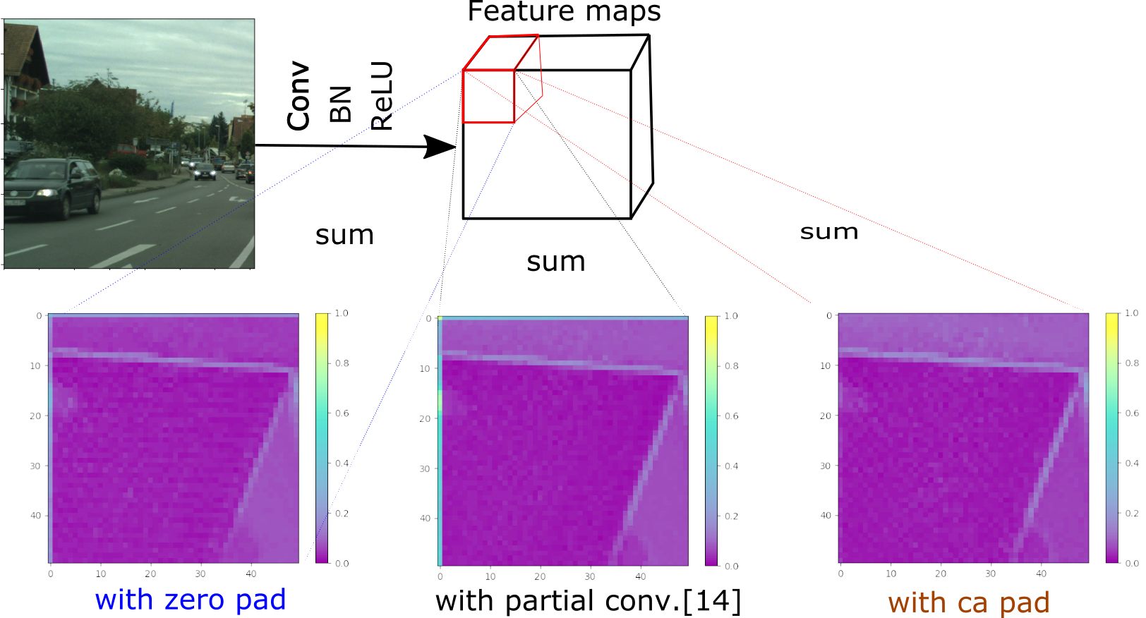
Figure 1: Visualization of a summed activation map from the convolution with different padding methods. We crop the top left corner of each one and normalize them to the same range. Compared to two other methods, CA-padding has more continuous boundary without any artifacts on the top/left border of summed activation map. (Best viewed by zooming in.)

In order to reduce border effects, one can apply other padding techniques such as reflection padding which reuses the value near the border in the reverse way or circular padding which has been applied in some specific setting [26]. Nguyen et al. [18] proposed a distribution padding to maintain the statistics of the border region. Alternatively, Liu et al. [14] proposed a re-weighting based scheme called partial convolution. Those methods contribute to a better performance in the classification and segmentation tasks, however, we observe that one research path remains unexplored.

In this paper, we introduce a novel context-aware padding approach, in short CA-padding. We reformulate the padding problem as an image extrapolation task, and train a separate network to predict the area outside the image. Using this approach, we intend to improve the existing methods by including more realistic statistics. Since the information in the image level will be propagated through layers to the end, we consider it is important to understand what the network receives in the beginning. Therefore, we start with predicting the padding for the first layer of convolutional neural networks.

In the context of image extrapolation, the use of generative adversarial networks (GANs) would naturally come to mind. They are quite popular as they have shown to generate realistic results. There have also been works using multi-stage processes to improve the results even further. Related approaches tackle the image extrapolation task by means of autoregressive models. However, using such generative models in our context, would bring quite some computational overhead. These methods are typically based on a much more complicated architecture, and require longer inference time, thus are less attractive when using high resolution images.

Our method saves the computation time by only taking local region to directly predict the displacement to extrapolate the image. Furthermore, it does not require a heavy network and the computation is executed in the local region instead of the whole image and thus make it efficient. Also, for different spatial regions, we train separate networks to have them focused on the right information. At run time these models are executed in parallel as there is no dependency between them.

We evaluate our proposed padding model on top of state-of-the-art segmentation models on two different semantic segmentation datasets. One for autonomous driving and one for satellite image recognition. The main contributions of this paper can be summarized as follows:

1. A simple neural network to perform image extrapolation as a padding method for the convolution layers.

2. The neural network based model behaves better than the naive padding approaches, since it exploits the context information and therefore its prediction is closer to the real statistics.

3. We study the effects of the proposed padding method in the context of semantic segmentation, and compare with other methods.

2 Related Works

In this section, we briefly introduce the related works in the following categories, semantic segmentation, padding and image extrapolation.

2.1 Semantic segmentation

Starting from fully convolutional neural networks (FCN) [17], the semantic segmentation task has been effectively tackled by deep neural networks. Following this work, researchers mostly focused on either integrating more context information in the network, which helps to disambiguate local information, or using local cues to arrive at better spatial predictions. The amount of research is vast and it includes the use of encoder-decoder architectures [1, 4], dilated or atrous convolutions [31, 2], pyramid pooling modules [36], squeeze-and-excitation modules [10], multi-scale predictions [7, 35], attention models [3], feature fusion [15, 20], context modules [33, 32], etc. The reader can refer to [8] for a review on some of aforementioned semantic segmentation techniques. At their core, however, all these approaches leverage the great representational power of deep models, like [9], trained on large datasets of fully-annotated images, like [13, 5], to achieve impressive results. In this paper, our focus is not the exact architecture for semantic segmentation. Rather we want to investigate the impact of padding on the segmentation performance. Hence the underlying idea is as well that the proposed method can be applied to any of aforementioned models.

2.2 Padding

In addition to zero padding, there are different kinds of padding applied such as circular padding or reflection padding under the context of signal processing. For reasons of efficiency, there is a tendency to use zero padding in convolutional neural networks rather than other types of padding. In the recent years, padding gained some more interest though. Liu et al. [14] proposed the partial convolution and it was also applied to tackle the image inpainting task. It is done by re-weighting the results from convolution layers near the image border based on the ratio between the padding area and the convolution sliding window area. Later on, Nguyen et al. [18] proposed a mean distribution padding method to replace zero padding for classification and image generation task. In this way, they try to keep the same statistics on the border to avoid the border effect. In the special case of even-sized kernels, Wu et al. [27] proposed to apply symmetric padding. Triess et al.  [23] utilized cyclic padding to provide more context when processing the LiDAR points. As opposed to these methods, our method uses the context information to provide a better padding prediction.

2.3 Image extrapolation

Image extrapolation or image outpainting refers to the task of predicting the region beyond the borders of a given image. Prior to the success of the deep neural networks, the missing parts in the images were filled by retrieving similar patches from the input image [34, 12] or other images of a large database [25]. Since the success of generative adversarial models (GANs), a few learning-based methods have been designed for indoor 3D structure [21] or human body images [28]. Recently, Wang et al. [29] proposed a semantic regeneration network which first expands the feature and then predicts the extended image. Teterwak et al. [22] improves the discriminator with semantic conditioning to generate a more semantic coherent extensions. Yang et al. [30] utilizes recurrent mechanism to keep the content consistent for long natural scenery image extension. In addition to GANs based methods, there is another type of model for image generation, autoregressive models. Models such as PixelRNN [19], PixelCNN [24] and so on are typical examples. These generative methods can generate plausible results, but, as indicated in the introduction, they would bring additional overhead (training effort, inference time, architecture size, etc) on their use in this particular padding setting.

In this paper, we provide a simple but accurate enough method for image extrapolation. It does not need multi-stage training and is easy to be integrated into e.g. a segmentation model.

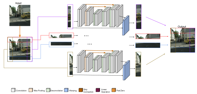
Figure 2: The pipeline of our context-aware padding model.

3 Method

Here we explain our padding approach. As mentioned earlier, since padding is an essential component in a convolutional neural network, the additional overhead due to the padding process itself should be kept to a minimum, and hence we want to avoid that the practical use of the method would be compromised by the increase in training (and inference) time. Therefore we aim to find a balance between the accuracy of the padding model and its efficiency.

3.1 Image level padding

We model the image padding problem as a ’local’ image extrapolation problem. Given an RGB image $I$ with the shape ($h,w$), the goal is to have a model $T$ to predict a spatialwise extended image $I^{\prime}$ where the size of $I^{\prime}$ equals to the shape of $I$ plus two padded areas on each of the vertical (height) or horizontal (width) sides of $I$. Suppose we set the amount of padding in the convolution layer $l$ to $p$. This is equivalent to taking an image of size ($h+2*p,w+2*p$) as the input to $l$ with no further padding during the convolution computation.

In order to save GPU memory, we only use the regions nearby the border to predict the padding values. For each side of the image, we train separate padding prediction model. Take the left side for example. We first crop the left $m$ pixels from the image, append $p$ of zeros at the left side of the crop and thus form a new block $b$ with the size ($h,p+m$). The block $b$ serves as the input to our padding model.

Our padding prediction model is inspired by [16], and is composed of two parts,

• a displacement network, based on a simple encoder-decoder architecture with skip connections.

• a warping layer.

The architecture is also illustrated in Fig. 2. Given a local region $b$ as input, the encoder-decoder $E$ predicts a pixelwise displacement $F$ which gives an idea on how the padding (border) area is correlated to the central part. Then the warping layer $T$ exploits the predicted displacements to fill in the padding area using the input pixels.

$$F=E(b,W)$$ (1)

where $W$ denotes the network parameters of $E$. For every pixel $(x_{i},y_{i})$ in $b$, the coordinates w.r.t. the ones after transformation $(x_{i}^{warp},y_{i}^{warp})$ are associated as,

$$x_{i}=x_{i}^{warp}-\Delta x_{i},y_{i}=y_{i}^{warp}-\Delta y_{i}.$$ (2)

, where $(\Delta x,\Delta y)$ denotes the displacement vectors predicted from the decoder.

With the warping layer, the output image $b^{\prime}$ is formulated as,

$${b^{\prime}}_{i}=\sum_{k\in N(x_{i},y_{i})}b_{k}(1-|x_{i}-x_{k}|)(1-|y_{i}-y_{k}|),$$ (3)

, where ${b^{\prime}}_{i}$ denotes the value of the $i$-th pixel at $(x_{i}^{warp},y_{i}^{warp})$ in the output $b^{\prime}$, and $N(x_{i},y_{i})$ is the 4-neighborhood region of the pixel at $(x_{i},y_{i})$ in the input $b$.

3.2 Reconstruction Loss

The reconstruction loss for the training process is defined as follows. Suppose, after the data augmentation, we obtain an image crop $b$. This image crop serves as the ground truth for the image extrapolation. We then apply a binary mask $M$ to the image crop, to mimic the border effect. The resulting image is set to be the input of our padding model $T$. In the mask, we set the value of the padding region to 0 and 1 for other known region. To train the model, we optimize the following reconstruction loss.

$$L=\frac{1}{N}\sum_{b\in D}(\|b\odot(1-M)-T(b\odot M,F)\odot(1-M)\|)$$ (4)

where $D$ is the training set, $N$ is its cardinality.

3.3 Feature level padding

The method described for image level padding applies to feature level padding as well. To generate the ground truth feature maps for training, we extract intermediate features from a pre-trained segmentation network. We then apply the mask $M$ on top of it as described in the previous section to generate the input to the network. However, during the experiments we found that adding additional CA-padding to feature level gives only marginal improvement which does not weigh up against the additional computation overhead.

4 Experiments

Datasets We use Cityscapes and the dataset from the DeepGlobe Land Cover Classification Challenge [6] to test our method.

• In the Cityscapes dataset, there are 5,000 images with fine pixelwise annotation collected by driving a car in 50 cities in different seasons. Those images are divided into train/ validation/ test set with 2,975/ 500/ 1,525 number of images. Each image has a resolution of 1024 by 2048 pixels. The dataset is annotated for 19 classes.

• The dataset from the DeepGlobe challenge consists of 1,146 high-resolution satellite images. There are 803 / 171 / 172 images in the training / validation / testing set. Each image has corresponding pixelwise class labeled image with seven different classes including urban land, agriculture land, rangeland, water, barren land and unknown class.

In the experiments, we adopted the datasets’ training set for training, and used the corresponding validation set for evaluation. The evaluation is done in single-scale without flipping the input image.

Metric To evaluate the segmentation performance, we follow the convention to compute the mean of class-wise intersection over union (mIoU).

Training Details We optimize the padding model using the Adam algorithm [11] with learning rate 1$\times{10}^{-4}$ and (${\beta}_{1},{\beta}_{2})=(0.9,0.999)$. The batch size is 8 and we train it for 150 epochs. For data augmentation, we apply the same one as for semantic segmentation model training. To be more specific, we adopt random mirror, random resize between (0.5, 2), random rotation between (-10, 10) degrees, random Gaussian blur and random crop to a specific size.

For segmentation, we optimize the model with SGD with initial learning rate of 1e-2 and poly learning rate. To train the model, we apply data augmentation as described in the previous paragraph. For both datasets, we crop the image to 713 by 713. To test the model, we follow the same strategy as PSPNet by using the overlapping crops of the size 713 by 713. For other padding models, we adopt the same setting except for replacing the padding.

For comparison, we followed the steps described in [14] to train the baseline model with partial convolution. That is, we replaced all the convolution layers with the partial convolution in the encoder. In the case of PSPNet, it includes the backbone architecture and the pyramid pooling module. In addition, we implement the mean interpolation padding from [18] as another related work. For a fair comparison, we also include other padding methods (replication, reflection and bilinear interpolation) under the same setting as ours which is to replace the first zero padding of the network.

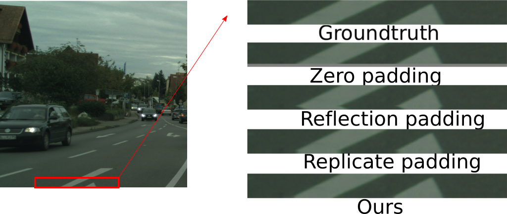
Figure 3: The results for the different padding methods is illustrated here on the cropped area within the red bounding box. The effect of the padding is visible in the bottom row of the images.

4.1 Padding evaluation

To simulate the padding in convolution layers during training the segmentation model, we use the same data augmentation that is used for training the segmentation model itself. We apply overlapping crops and take the border region as ground truth to evaluate different padding methods. We train our padding model using the training set and evaluate the padding performance on the validation set. We take an image and multiply it by a 0-1 mask to create the input of our model. The image before masking acts as the ground truth for our padding model.

To estimate the effect of our image padding model, we compare our models with other padding methods, including zero padding, circular padding, reflect padding, replicate padding and the padding by directly bilinear interpolation. Table 7 and Table 6 presents the results on Cityscapes and the DeepGlobe dataset. For both dataset, we crop the input image to 719 by 719 pixels in a sliding window fashion. Each crop has one third overlapping with the previous crop. The notation $pad_{i}$ means we pad $i$ pixels at each side of image. In both cases, we take 20 pixels wide region to predict the padding. The results show that our method performs better than any of the other padding models in both PSNR and MSE metrics. In general, the results of the $pad_{3}$ are always worse than $pad_{1}$ because the further it is to the known region the less information is provided. Among all other padding methods, replicate padding behaves best, but is still slightly worse than our model.

Fig. 3 illustrates an example of different padding. The left part shows an image after padding with 3 pixels at each side. In the right part, we zoom in the region specified by the red box and present the cases for different padding. We can see that from the reflection and replicate padding, the pattern of the sign becomes different. From this, we can infer that if there is object with specific structure on the border of the image, the reflection padding and replicate padding will change the pattern.

4.2 Segmentation Results

We first compare our padding method with our state-of-the-art methods by replacing the padding method for the first convolution layer in the ResNet50. And the padding for other layers keep the zero padding. For comparison, we replace the convolution layers from the baseline with partial convolutions. Table 1 presents the segmentation results in mIoU for different padding methods. From the table, we can see partial convolution improves the baseline zero padding method by 0.8%. On top of that, our padding brings 0.1% improvement more than partial convolution. Though from the previous section the replicate padding shows good performance, it only brings 0.2% improvement when it applies to the segmentation model. Among 19 classes, ours achieves the highest performance in 14 classes. To be noted that, for some classes of small object like pole,bike and motorbike, our padding method brings around 1 to 4% improvement compared to the baseline. It might be because our padding method can generate the extension more closed to the real pattern rather than just filling in zero when an object lies on the border.

To evaluate how well our model improves at the boundaries, we test different crop size during evaluation. Fig. 4 shows corresponding segmentation results. As we can observe from the figure, the smaller the crop size is, the more our CA-padding outperforms the baseline model (from +0.9% to +1.8%) due to more boundaries involved.

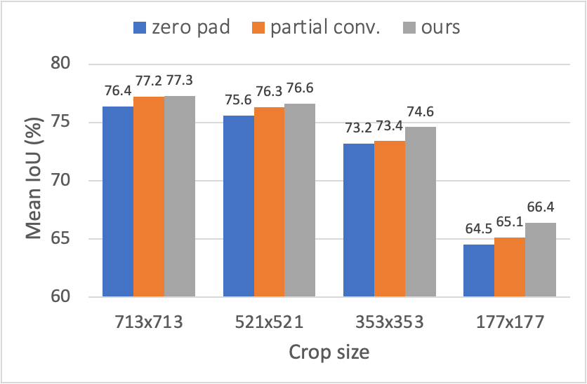
Figure 4: The segmentation result on Cityscapes val set with different padding models using different crop size during testing.

Method	road	swalk	build	wall	fence	pole	tlight	tsign	veg.	terrain	sky	person	rider	car	truck	bus	train	mbike	bike	mean
zero	97.9	83.6	92.1	51.9	59.0	62.8	69.5	77.0	92.2	63.7	94.4	81.1	60.6	94.7	76.1	84.5	71.4	63.2	76.6	76.4
partial conv	97.9	84.1	92.1	53.3	59.2	62.9	69.6	77.3	92.4	66.6	94.1	81.3	60.9	94.6	76.4	87.3	74.6	65.4	76.6	77.2
dist [18]	96.9	77.9	90.0	41.4	52.9	56.5	62.7	72.6	91.1	57.3	93.3	77.3	52.5	92.8	62.3	71.5	62.0	60.4	74.1	70.8
replicate	97.7	82.1	92.0	55.4	58.1	61.9	69.1	76.5	92.4	65.4	94.2	81.2	59.1	94.5	74.2	86.8	72.9	64.1	76.4	76.6
bilinear	97.9	83.5	92.1	52.9	58.8	63.4	69.9	77.3	92.4	64.1	94.5	81.5	60.5	94.6	71.6	86.5	67.3	65.8	76.7	76.4
ours	97.9	83.5	92.1	56.2	59.5	63.5	69.9	77.3	92.4	65.1	94.4	81.6	60.9	94.6	74.5	88.4	73.9	66.7	77.2	77.3

Table 1: Segmentation results in classwise IoU of the PSPNet with ResNet50 backbone on Cityscapes val dataset. ”dist” denotes distribution padding and ”bilinear” denotes bilinear interpolation.

We further test our padding model with a deeper backbone, ResNet101, on Cityscapes. Table 2 presents corresponding mean IoU for different padding methods. From the result, we can see our padding still improves the baseline by similar amount of mean IoU as ResNet50. It shows the eligibility of our model. Differently, the model with partial convolution has less improvement compared with the version with ResNet50 backbone. This shows that the weight rescaling method from partial convolution might disturb the learning when the network goes deeper.

Method	road	swalk	build	wall	fence	pole	tlight	tsign	veg.	terrain	sky	person	rider	car	truck	bus	train	mbike	bike	mean
zero	98.0	84.3	92.4	57.2	59.3	61.9	70.2	77.6	92.6	65.6	94.4	82.2	62.7	94.8	74.5	85.5	76.3	64.6	77.5	77.4
partial conv.	98.0	84.5	92.2	54.5	59.8	63.5	70.7	78.0	92.4	63.9	94.4	82.0	61.7	95.0	79.3	88.6	78.6	63.4	77.5	77.8
ours	97.9	84.3	92.5	59.7	60.4	64.1	71.0	77.7	92.5	64.7	94.4	82.1	62.8	94.9	78.9	89.5	78.6	68.1	77.9	78.5

Table 2: Segmentation results in classwise IoU of the PSPNet with ResNet101 backbone on Cityscapes val dataset.

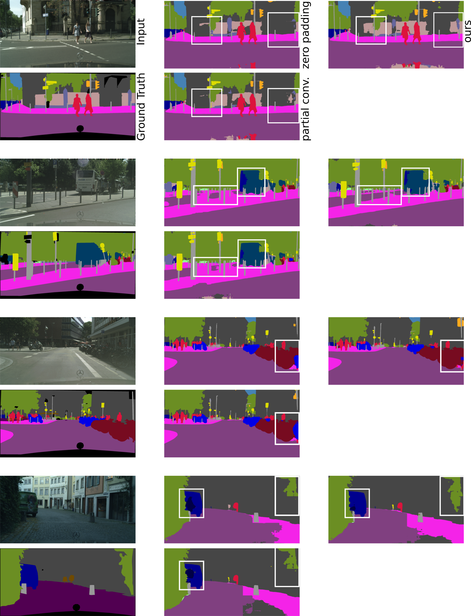
Figure 7: Qualitative results of PSPNet-ResNet101 with different padding, zero padding, partial convolution and our padding model.

Fig. 7 illustrates the segmentation results on Cityscapes validation set. The baseline zero padding model is trained with PSPNet-ResNet101. From the first row of the figure, the model with our CA-padding successfully predicts the fence on the left and right border of the image. Additionally, our model clearly delineates the road between the sidewalks from the example of the second row. The improvement is not only found on the borders but also closed to the center of image because the learnt filters are shared across the image. Therefore, a better padding method is helpful for learning better representation.

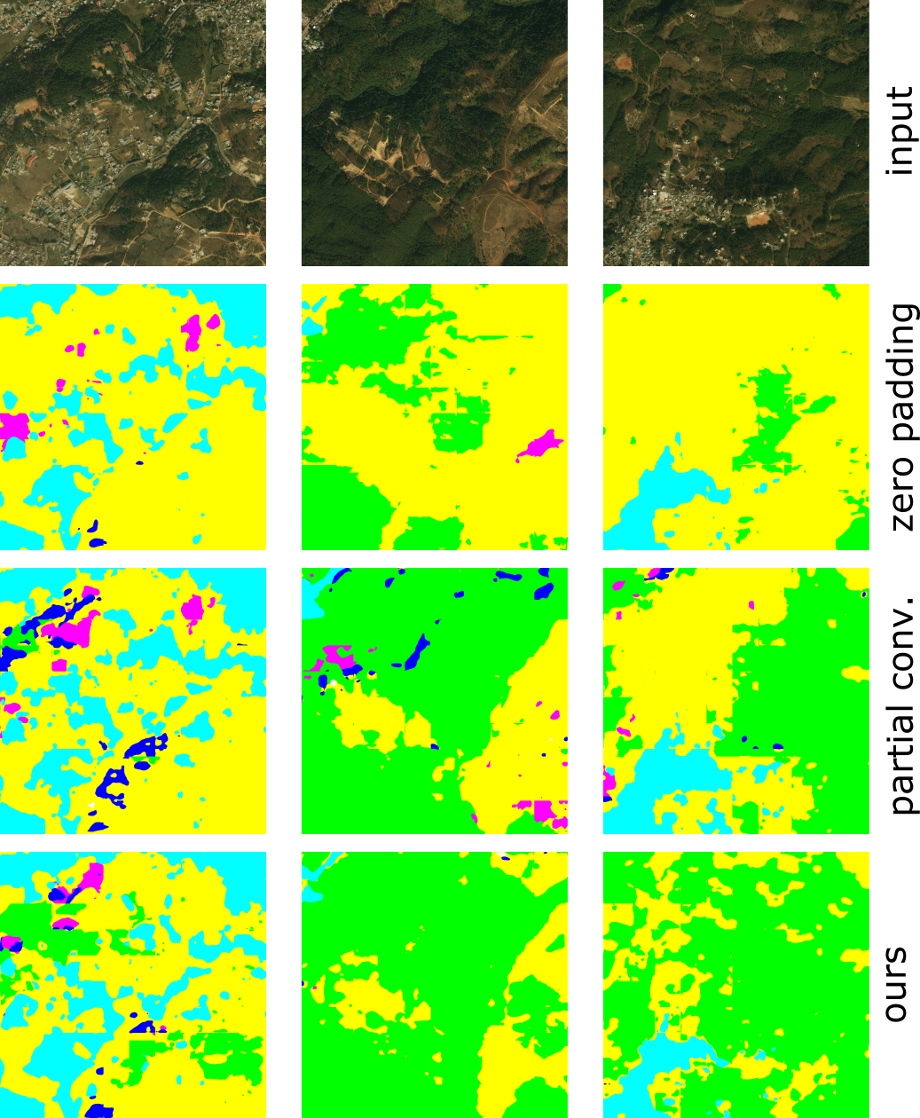
Figure 8: Qualitative results of PSPNet-ResNet18 on the DeepGlobe val set. with different paddings : zero padding, partial convolution and our padding model. Colors: urban, agriculture, rangeland, forest, water, barren, unknown.

To test our padding model in different type of scene other than driving, we perform experiments on a dataset from DeepGlobe Land Cover Classification Challenge. We take the PSPNet with ResNet18 as backbone as our baseline. Because the label of validation set is not available, we randomly choose 171 images from the training set to select our final model. Table 3 presents the result on the official validation set received from the evaluation server. Our CA-padding outperforms the baseline zero padding method by around 2.5% which is one to four percent more than partial convolution and replicate padding respectively. Fig. 8 illustrates the segmentation results with different padding models on DeepGlobe validation set.

Method	mean IoU
zero padding	45.20
partial conv.	45.88
distribution padding	42.30
replicate padding	43.24
bilinear interpolation	42.03
ours	47.84

Table 3: Evaluation of different padding method with PSPNet-ResNet18 on the DeepGlobe dataset validation set.

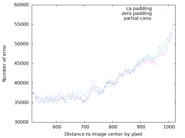
Figure 5: Error plot for the ResNet-101 on Cityscapes validation set. The x-axis is the distance to the image center and the y-axis is the number of error.

As indicated in section 3, it is possible to apply the CA-padding principle on feature level as well. During the experiments we found that adding additional CA-padding to feature level gives only marginal improvement. Whereas the CA-padding on image level increase the segmentation performance up to $77.3$, including additional CA-padding on the feature levels increases the performance up to $77.5$. As explained in section 4.5, it would further add additional overhead on the computational time, proportional to the amount of layers.

4.3 Error Analysis

To further understand the effect of our CA-padding on semantic segmentation compared to the zero padding, we plot the error distribution according to the distance to the image center. In this analysis, we take PSPNet with ResNet101 backbone as our baseline and evaluate the performance on Cityscapes validation set. We exclude the labels which do not count in the official evaluation (ignore labels). For each pixel of the prediction, we compare it with corresponding pixel from the ground truth label and create an error plot as shown in Fig. 5 . Here we plot the distance of the pixels to the image center (x-axis) against the amount of pixels for which the ground truth labels and predicted labels differ. Fig. 5 illustrates this plot with three different settings, zero padding, CA-padding and partial convolution. It can be observed that the number of error achieves the maximum at around 1,000 pixel away from the center. We further zoom in the region from pixel 800 to 1,000, we can see that in most of the time the CA-padding (green dots) has least number of error. The second least is the partial convolution (blue dots) and then the zero padding (purple dots). From the result, we can infer that the distribution near the border region is improved by our CA-padding so that the number of error decreases compared with other padding methods.

Finally, in order to understand the performance close to the border region, we follow [14] to evaluate the segmentation performance in the mean IoU metric on border regions. It is done by excluding the center regions when computing the mIoU. Fig. 6 illustrates examples of different proportions leaving out from the center regions. We set the center ($\frac{1}{3}\times\frac{1}{3}$, $\frac{1}{2}\times\frac{1}{2}$ ,$\frac{2}{3}\times\frac{2}{3}$, $\frac{3}{4}\times\frac{3}{4}$) to ”don’t care” labels in the ground truth. Table 4 shows the results on the Cityscapes dataset. From the table, we can observe that when the leaving-out ratio goes higher, we obtain a better mean IoU. But when the ratio is larger than $\frac{1}{2}\times\frac{1}{2}$, the performance drops for all the cases. For the case of $\frac{3}{4}\times\frac{3}{4}$, both partial convolution and our padding improve the most compared to zero padding. The corresponding improvements are 0.43% and 1.95%.

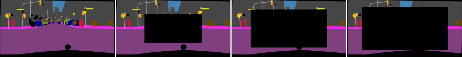
Figure 6: Examples of segmentation map with different leave-out proportion from the center regions.

Method	0	$\frac{1}{3}\times\frac{1}{3}$	$\frac{1}{2}\times\frac{1}{2}$	$\frac{2}{3}\times\frac{2}{3}$	$\frac{3}{4}\times\frac{3}{4}$
zero	77.53	78.74	79.57	79.14	78.06
partial conv.	77.88	78.95	79.63	79.27	78.49
ours	78.62	79.66	80.52	80.36	80.01

Table 4: Evaluation of different proportions of center region leaving out on Cityscapes dataset. Further details can be found in Sec. 4.3.

4.4 Ablation Study

Here we explore different designs for our padding model. Size of input region We further explore the size of input region to see if further context is useful to predict the displacement. Table 5 shows the MSE metrics with 20 and 30 pixels out of 713 pixels from the input. From the PSNR and MSE, given more region as the input seems not help. So we keep the design of 20 pixel to predict the padding.

size of input	PSNR	MSE
20 / 713 pixels	49.27	5.41e-05
30 / 713 pixels	49.19	5.46e-05

Table 5: Quantitative results for the padding prediction with different range of region given as input to the network evaluated on the Cityscapes val set.

4-direction model needed? In the design of our padding model, we separated the training in four different directions, left, right, top and down (cfr Fig. 2). To test if it is necessary to train four models separately, we evaluate the padding only with the left and top model. In this setting, we use the left model to predict both left and right padding. The input from the right border is first flipped horizontally and sent to the left model. The same applies to the top model. We predict the top and bottom padding with the top model. We follow the same evaluation steps as in Section 4.1 and calculate the PSNR and MSE. The corresponding numbers are 43.64 and 0.0002. Compared with the one trained with four different model from Table 6, the PSNR drops around six and the MSE becomes ten times more. As a result, it proves the necessity of having four independently trained models for each direction.

4.5 Training Time Overhead

We measure the training time per epoch on a machine with four NVDIA V100 GPU for different padding. We take PSPNet with ResNet101 as our baseline (with all zero padding). On Cityscapes dataset, the baseline method takes about 233.873 second for one epoch training. After adding our CA-padding, the training time per epoch becomes 244.133 second. It increases 10.26 second for one epoch which is 4.3% increase compared to the baseline. Similar range of overhead applies to testing time as well. As a comparison, we also measure the training time for partial convolution. For one epoch, it takes 241.119 second which is a bit faster than our CA-padding but our method can bring further improvement. Noted that the run time will decrease if we further parallelize our method.

Convergence Speed During training, we evaluate the model on validation set after each epoch. For each image in the validation set, we crop from the center a specific size. For total 200 epoch of training, we set a threshold on mean IoU to see which number of epoch can the model achieve. For the PSPNet-ResNet101 training on the Cityscapes dataset, the baseline model takes 148 epochs to achieve 76% mIoU. The model with partial convolution and with CA-padding takes 136 / 117 epochs to achieve similar result separately. It shows that our CA-padding can help converge faster than the baseline model and the model with partial convolution. To summarize, our model always achieves the highest performance, regardless the amount of epochs one chooses to train any of the alternative methods.

	${pad_{3}}$		$pad_{1}$
model	$PSNR$	$MSE$	$PSNR$	$MSE$
zero padding	29.10	3.9e-03	33.85	1.3e-03
bi. interpolation	28.85	2.0e-04	29.92	5.5e-05
circular padding	31.92	3.2e-03	36.66	1.1e-03
reflect padding	44.75	2.0e-04	53.27	2.1e-05
replicate padding	48.40	6.6e-05	57.82	7.5e-06
$ours$	49.17	5.51e-05	58.62	6.4e-06

Table 6: Quantitative results for the padding prediction with padding size three and one on Cityscapes val set.

model	$PSNR$	$MSE$
zero padding	31.04	0.0036
bilinear interpolation	26.28	0.0003
circular padding	35.16	0.0015
reflect padding	41.79	0.0003
replicate padding	44.00	0.0002
$ours$	44.48	0.0002

Table 7: Quantitative results for the padding prediction with padding size three on the DeepGlobe val set.

5 Conclusions

We proposed a context-aware (CA) padding method by transforming the nearby pixel to predict the padding value. Compared with the traditional generative models, our model is light-weight and easy to train. We explore the application of our padding model on semantic segmentation tasks. Compared with traditional padding methods, ours improves the state-of-the-art PSPNet on Cityscapes and a satellite imaging dataset.

Acknowledgments We gratefully acknowledge the support of the TRACE project with Toyota TME.

References

- [1] Vijay Badrinarayanan, Alex Kendall, and Roberto Cipolla. Segnet: A deep convolutional encoder-decoder architecture for image segmentation. arXiv preprint arXiv:1511.00561, 2015.
- [2] Liang-Chieh Chen, George Papandreou, Iasonas Kokkinos, Kevin Murphy, and Alan L Yuille. Deeplab: Semantic image segmentation with deep convolutional nets, atrous convolution, and fully connected crfs. IEEE transactions on pattern analysis and machine intelligence, 40(4):834–848, 2018.
- [3] Liang-Chieh Chen, Yi Yang, Jiang Wang, Wei Xu, and Alan L Yuille. Attention to scale: Scale-aware semantic image segmentation. In Proceedings of the IEEE conference on computer vision and pattern recognition, pages 3640–3649, 2016.
- [4] Liang-Chieh Chen, Yukun Zhu, George Papandreou, Florian Schroff, and Hartwig Adam. Encoder-decoder with atrous separable convolution for semantic image segmentation. arXiv preprint arXiv:1802.02611, 2018.
- [5] Marius Cordts, Mohamed Omran, Sebastian Ramos, Timo Rehfeld, Markus Enzweiler, Rodrigo Benenson, Uwe Franke, Stefan Roth, and Bernt Schiele. The cityscapes dataset for semantic urban scene understanding. In Proceedings of the IEEE conference on computer vision and pattern recognition, pages 3213–3223, 2016.
- [6] Ilke Demir, Krzysztof Koperski, David Lindenbaum, Guan Pang, Jing Huang, Saikat Basu, Forest Hughes, Devis Tuia, and Ramesh Raskar. Deepglobe 2018: A challenge to parse the earth through satellite images. In The IEEE Conference on Computer Vision and Pattern Recognition (CVPR) Workshops, June 2018.
- [7] David Eigen and Rob Fergus. Predicting depth, surface normals and semantic labels with a common multi-scale convolutional architecture. In Proceedings of the IEEE International Conference on Computer Vision, pages 2650–2658, 2015.
- [8] Alberto Garcia-Garcia, Sergio Orts-Escolano, Sergiu Oprea, Victor Villena-Martinez, and Jose Garcia-Rodriguez. A review on deep learning techniques applied to semantic segmentation. arXiv preprint arXiv:1704.06857, 2017.
- [9] Kaiming He, Xiangyu Zhang, Shaoqing Ren, and Jian Sun. Deep residual learning for image recognition. In Proceedings of the IEEE conference on computer vision and pattern recognition, pages 770–778, 2016.
- [10] Jie Hu, Li Shen, and Gang Sun. Squeeze-and-excitation networks. arXiv preprint arXiv:1709.01507, 7, 2017.
- [11] Diederik P. Kingma and Jimmy Ba. Adam: A method for stochastic optimization. In 3rd International Conference on Learning Representations, ICLR 2015, San Diego, CA, USA, May 7-9, 2015, Conference Track Proceedings, 2015.
- [12] Johannes Kopf, Wolf Kienzle, Steven Drucker, and Sing Bing Kang. Quality prediction for image completion. ACM Transactions on Graphics (Proceedings of SIGGRAPH Asia 2012), 31(6), 2012.
- [13] Tsung-Yi Lin, Michael Maire, Serge Belongie, James Hays, Pietro Perona, Deva Ramanan, Piotr Dollár, and C Lawrence Zitnick. Microsoft coco: Common objects in context. In European conference on computer vision, pages 740–755. Springer, 2014.
- [14] G. Liu, K. J. Shih, T.-C. Wang, F. A. Reda, K. Sapra, Z. Yu, A. Tao, and B. Catanzaro. Partial convolution based padding. arXiv:1811.11718, 2018.
- [15] Wei Liu, Andrew Rabinovich, and Alexander C Berg. Parsenet: Looking wider to see better. arXiv preprint arXiv:1506.04579, 2015.
- [16] Ziwei Liu, Raymond Yeh, Xiaoou Tang, Yiming Liu, and Aseem Agarwala. Video frame synthesis using deep voxel flow. In Proceedings of International Conference on Computer Vision (ICCV), October 2017.
- [17] Jonathan Long, Evan Shelhamer, and Trevor Darrell. Fully convolutional networks for semantic segmentation. The IEEE Conference on Computer Vision and Pattern Recognition (CVPR), 2015.
- [18] A.-D. Nguyen, S. Choi, W. Kim, S. Ahn, J. Kim, and S. Lee. Distribution padding in convolutional neural networks. ICIP, 2019.
- [19] Aaron Van Oord, Nal Kalchbrenner, and Koray Kavukcuoglu. Pixel recurrent neural networks. In Proceedings of The 33rd International Conference on Machine Learning, volume 48, pages 1747–1756, 2016.
- [20] Pedro O Pinheiro, Tsung-Yi Lin, Ronan Collobert, and Piotr Dollár. Learning to refine object segments. In European Conference on Computer Vision, pages 75–91. Springer, 2016.
- [21] Shuran Song, Andy Zeng, Manolis Savva Angel X. Chang, Silvio Savarese, and Thomas Funkhouser. Im2pano3d: Extrapolating 360 structure and semantics beyond the field of view. In CVPR, 2018.
- [22] P. Teterwak, A. Sarna, D. Krishnan, A. Maschinot, D. Belanger, C. Liu, and W. T. Freeman. Boundless: generative adversarial networks for image extension. ICCV, 2019.
- [23] L. T. Triess, D. Peter, C. B. Rist, and J. M. Zöllner. Scan-based semantic segmentation of lidar point clouds: An experimental study. IV, 2020.
- [24] Aaron van den Oord, Nal Kalchbrenner, Lasse Espeholt, koray kavukcuoglu, Oriol Vinyals, and Alex Graves. Conditional image generation with pixelcnn decoders. In Advances in Neural Information Processing Systems 29, pages 4790–4798, 2016.
- [25] M. Wang, Y.-K. Lai, Y. Liang, R. Martin, and S.-M. Hu. Biggerpicture: Data-driven image extrapolation using graph matching. ACM Trans. Graph, 2014.
- [26] Tsun-Hsuan Wang, Hung-Jui Huang, Juan-Ting Lin, Chan-Wei Hu, Kuo-Hao Zeng, and Min Sun. Omnidirectional cnn for visual place recognition and navigation. arXiv preprint arXiv:1803.04228, 2018.
- [27] S. Wu, G. Wang, P. Tabg, F. Chen, and L. Shi. Convolution with even-sized kernels and symmetric padding. NeuIPs, 2019.
- [28] Xian Wu, Rui-Long Liand Fang-Lue Zhang, Jian-Cheng Liu, Jue Wang, Ariel Shamir, and Shi-Min Hu. Deep portrait image completion and extrapolation. arXiv preprint arXiv:1808.07757, 2018.
- [29] Y. Wang and X. Tao and X. Shen and J. Jia. Wide-context semantic image extrapolation. CVPR, 2019.
- [30] Zongxin Yang, Jian Dong, Ping Liu, Yi Yang, and Shuicheng Yan. Very long natural scenery image prediction by outpainting. In Proceedings of the IEEE International Conference on Computer Vision, pages 10561–10570, 2019.
- [31] Fisher Yu and Vladlen Koltun. Multi-scale context aggregation by dilated convolutions. arXiv preprint arXiv:1511.07122, 2015.
- [32] Yuhui Yuan and Jingdong Wang. Ocnet: Object context network for scene parsing. arXiv preprint arXiv:1809.00916, 2018.
- [33] Hang Zhang, Kristin Dana, Jianping Shi, Zhongyue Zhang, Xiaogang Wang, Ambrish Tyagi, and Amit Agrawal. Context encoding for semantic segmentation. In Proceedings of the IEEE Conference on Computer Vision and Pattern Recognition, pages 7151–7160, 2018.
- [34] Y. Zhang, J. Xiao, J. Hays, and P. Tan. Framebreak: Dramatic image extrapolation by guided shift-maps. In 2013 IEEE Conference on Computer Vision and Pattern Recognition, pages 1171–1178, 2013.
- [35] Hengshuang Zhao, Xiaojuan Qi, Xiaoyong Shen, Jianping Shi, and Jiaya Jia. Icnet for real-time semantic segmentation on high-resolution images. arXiv preprint arXiv:1704.08545, 2017.
- [36] Hengshuang Zhao, Jianping Shi, Xiaojuan Qi, Xiaogang Wang, and Jiaya Jia. Pyramid scene parsing network. In IEEE Conf. on Computer Vision and Pattern Recognition (CVPR), pages 2881–2890, 2017.