Unbiased Elimination of Negative Weights in Monte Carlo Samples

Abstract

We propose a novel method for the elimination of negative Monte Carlo event weights. The method is process-agnostic, independent of any analysis, and preserves all physical observables. We demonstrate the overall performance and systematic improvement with increasing event sample size, based on predictions for the production of a W boson with two jets calculated at next-to-leading order perturbation theory.

1 Introduction

The LHC physics programme has entered an era of precision measurements. Such measurements demand equally precise theory predictions. To match this requirement, it is most often necessary to include at least next-to-leading order (NLO) perturbative corrections. For a number of processes, even higher fixed-order corrections, i.e. NNLO and NNNLO, have to be taken into account. In order to consistently combine virtual corrections, usually computed in $d=4-2\epsilon$ dimensions, and real corrections, obtained via numerical integration over four-dimensional momenta, one introduces subtraction terms which render each component finite, see for example Catani:1996vz ; Catani:2002hc .

Since one is usually interested in distributions, additional effects from parton showers and hadronisation have to be accounted for. Methods such as MC@NLO Frixione:2002ik and POWHEG Nason:2006hfa can be employed for matching parton showers and NLO fixed-order predictions. Depending on the phase-space region of interest, further resummation may be required. Examples include transverse momentum Collins:1984kg and high-energy resummation Fadin:1975cb ; Balitsky:1978ic . High-accuracy predictions for multi-jet observables are then obtained by merging exclusive event samples using e.g. the MEPS@NLO Hoeche:2012yf or UNLOPS Lonnblad:2012ix ; Lonnblad:2012ng approaches. Finally, the detector response to the generated events is simulated GEANT4:2002zbu .

Thanks to continuous improvements, modern general purpose event generators Alwall:2014hca ; Bellm:2015jjp ; Sjostrand:2014zea ; Bothmann:2019yzt render the inclusion of many of these corrections feasible for a large range of scattering processes. However, the improved accuracy comes at a significant cost in computing time. What is more, each of the individual calculational steps outlined above also increases the cost of all subsequent steps. The reason for this is that typically a number of negative-weight counterevents are generated, for instance for unitarisation or in order to prevent double counting. This implies that a much larger number of events has to be processed to reach the same statistical significance as for the case of purely positive-weight event samples. This problem is particularly pronounced in the final detector simulation step, which can take hours of CPU time for each event.

In general, the number of events that have to be forwarded to the detector simulation can be reduced by unweighting the event sample. Taking $W$ as the largest absolute event weight in the sample, an event with weight $w_{i}$ is rejected with probability $\mathbb{P}=1-|w_{i}|/W$ and otherwise assigned the new weight $w_{i}\to\operatorname{sgn}(w_{i})W$. If all event weights are positive, an unweighted sample of $N$ events has uniform weight $w_{i}=W$, which is ideal in the sense that the Monte Carlo uncertainty estimate for the cross section, $\langle\sigma\rangle=\sqrt{\sum_{i=1}^{N}w_{i}^{2}}$, is minimal among all samples with $N$ events and the same predicted cross section $\sigma=\sum_{i=1}^{N}w_{i}$. Conversely, a given precision goal can be reached with the smallest number of events.

This ideal case of completely uniform weights is no longer achieved as soon as negative weights appear. For a fractional negative weight contribution

$$r_{-}=-\frac{\sum_{w_{i}<0}w_{i}}{\sum_{i}|w_{i}|},$$ (1)

the number of events required for a given precision goal increases to

$$N(r_{-})=\frac{N(0)}{(1-2r_{-})^{2}}$$ (2)

relative to the required number $N(0)$ in the absence of negative weights, see also Danziger:2021xvr .

Consequently, there have been a number of recent efforts to reduce the fraction $r_{-}$ of the negative weight contribution. One avenue that is being explored is to optimise the event generation itself Frederix:2020trv ; Gao:2020vdv ; Bothmann:2020ywa ; Gao:2020zvv ; Danziger:2021xvr . An alternative approach is to remove negative weights from the generated samples, while taking care that observables are not affected Andersen:2020sjs ; Nachman:2020fff ; Verheyen:2020bjw . The algorithm proposed in Andersen:2020sjs has been shown to be very effective in a highly non-trivial example. However, there are two caveats. First, the algorithm requires the choice of an auxiliary distribution, despite being process-agnostic in nature. Second, while the algorithm has been shown to produce sound results in practice, a proof of the correctness has only been given for a specific set of observables related to the chosen distribution.

In the following, we present a novel method, dubbed cell resampling, which eliminates negative event weights locally in phase space, is independent of the underlying process, and preserves all physical observables. Following the earlier proposal Andersen:2020sjs , we insert an additional resampling step before unweighting and detector simulation into the event generation chain outlined above. This step only affects the event weights, leaving all other properties untouched. Barring exact cancellations between weights, the number of events remains the same as well. We describe our method in section 2, and apply it to a calculation of W boson production with two jets at next-to-leading order in section 3. While we mostly focus on the application to fixed-order QCD generation of weighted event samples, the approach is largely independent of the details of the event generation, and we comment on possible generalisations whenever we have to make specific choices. We conclude with a summary and an outlook in section 4.

2 Cell Resampling

Our main goal is to eliminate negative event weights without affecting predictions for observables. We only consider observables that can be both predicted faithfully by a given event generator and measured in a real-world experiment involving detectors with a finite resolution.

To measure an observable $\mathcal{O}$ we first select a phase-space region $\mathcal{D}$ that is large enough to be resolved in a real-world experiment, where the resolution is typically limited not only by the detector, but also by the available statistics. The measured value of the observable is then obtained by counting events within this region. Obviously, this will always yield a non-negative result.

On the theory side, we predict the value of the observable from a Monte Carlo event sample with both positive and negative weights by summing up the weights $w_{i}$ of the events $i$ contained in the selected region $\mathcal{D}$:

$$\mathcal{O}=\sum_{i\in\mathcal{D}}w_{i}.$$ (3)

Since this corresponds to a Monte Carlo estimate of the integrated physical cross section over the selected phase space region, the result has to be non-negative given enough statistics.

We now aim to modify the event weights in such a way that negative weights are eliminated. At the same time, predictions for any observables of the kind discussed above should be preserved. To this end, we focus on a single event with negative weight, our seed, and consider a small solid sphere in phase space that is centred around said event and contains no other events. We call this sphere a cell. We then gradually increase the radius of the cell until the sum over all weights of events contained inside the cell is non-negative.

The key point is that with sufficiently many generated events, this cell can be made arbitrarily small. In particular, it can be made so small that it cannot be resolved anymore in a real-world experiment. At this point, we may freely redistribute the weights of the events within the cell without affecting any observables. One possible choice is to replace all event weights by their absolute value and rescale them such that the sum of weights is preserved. That is, we perform the replacement

$$w_{i}\to\frac{\sum_{j\in\mathcal{C}}w_{j}}{\sum_{j\in\mathcal{C}}|w_{j}|}|w_{i}|$$ (4)

for all weights $w_{i}$ of events $i$ inside the cell $\mathcal{C}$. This accomplishes the original intent behind the generation of negative-weight counterevents: any overestimation of the cross section from positive-weight events is cancelled locally in phase space.

After applying the above steps successively to each negative-weight event we are left with a physically equivalent sample of all positive-weight events. While it is in principle possible to apply the procedure to unweighted events, this would needlessly inflate cell sizes and systematically discard all events inside a cell, since their weights would sum up to zero. We therefore assume weighted input events. If desired, efficient unweighting can be performed after the elimination of negative weights.

Note that the method is completely agnostic to any details of the event generation, including the underlying process, and does not refer to any properties of specific observables. The only prerequisite is sufficiently high statistics, so that single cells are not resolved by any observable that can be measured in a real-world experiment.

In practice, it may not be feasible to generate and resample enough events to reach this goal. A particular concern is posed by cells containing events in different histogram bins of some distribution. Small enough cells close to bin boundaries can even turn out to be beneficial by smoothing out statistical jitter due to bin migration. However, as cells grow larger, the resampling will start to smear out characteristic features, such as resonance peaks.

To ensure that smearing effects remain negligible compared to other sources of uncertainty we can impose an upper limit on the cell sizes. The cost we have to pay is that some cells may not contain sufficient positive weight events to cancel the contribution from events with negative weight. This implies that we no longer eliminate all of the negative event weights. Still, since at least part of the negative seed event weight is absorbed by surrounding events, a subsequent unweighting will reduce the fraction of negative-weight events compared to the original sample. The size of cells with negative accumulated weight is related to the extent in phase space of counter-terms, and as such is related to the usual problems with bin-to-bin migration in higher-order calculations.

For the sake of a streamlined presentation, we will allow cells to grow arbitrarily large for the remainder of this section. We will come back to the discussion of a cell size limit when analysing the practical performance of our method in section 3.

2.1 Distances in Phase Space

A central ingredient in cell resampling is the definition of a distance function in phase space. While it may be possible to achieve even better results with functions tailored to specific processes and observables, our aim here is to define a universal distance measure.

There are two main requirements. First, let us consider events which are close to each other according to our distance function. Such events will very likely be part of the same cells and redistribute weights among each other. It is therefore absolutely essential that they have similar experimental signatures or only differ in properties that are not predicted by the event generator. Otherwise it is possible that only some of these events contribute to a given observable and the total weight of this subset and therefore the prediction for the observable is changed by the resampling. Second, it is desirable that events with a large distance according to the chosen function are easily distinguishable experimentally. In short, the distance function should reflect both the experimental sensitivity and the limitations of the event generator.

One consequence of these requirements is that the distance function has to be infrared safe. Adding further soft particles to an event should only change distances by a small amount. Specifically, final-state particles with vanishing four-momentum are undetectable and should not affect distances at all. Furthermore, the distance function has to have limited sensitivity to collinear splittings as well as soft radiation. In general, this can be achieved by basing the distance function on suitable defined infrared-safe physics objects instead of the elementary particles in the final state. The precise definition of these physics objects may depend on the details of the theory prediction. In the following, we consider only pure QCD corrections and ensure infrared safety by considering final-state jets instead of partons. It is natural to adopt the same jet clustering that was used for the event generation.

Keeping the general requirements in mind, we now define a concrete distance function for use with fixed-order Monte Carlo generators, which we use in the following. Note that our choice is by no means unique and we do not claim that our definition is optimal. A particularly promising alternative is the “energy mover’s distance” introduced in Komiske:2019fks and generalised to include flavour information in Romao:2020ojy . We leave a detailed comparison between different distance functions to future work.

2.1.1 Definition of the Distance Function

As a first step, we cluster the partons in each event into jets. We then group outgoing particles into sets according to their types, i.e. according to all discrete observable properties such as flavour and charge. Here, we are using the word “particle” in a loose sense, designating a jet — or, more generally, any infrared-safe physics object — as a single particle. Particles which only differ by their four-momenta (including possible differences in their invariant masses) end up inside the same set. For the time being, we do not differentiate between polarisations or various types of jets, but it is straightforward to add such distinctions.

The distance $d$ between an event $e$ with $T$ particle type sets $\mathcal{S}=\{s_{1},s_{2},\dots,s_{T}\}$ and an event $e^{\prime}$ with sets $\mathcal{S^{\prime}}=\{s_{1}^{\prime},s_{2}^{\prime},\dots,s_{T}^{\prime}\}$ is then given by the sum of the distances between matching sets, i.e.

$$d(e,e^{\prime})=\sum_{t=1}^{T}d(s_{t},s_{t}^{\prime})\,,$$ (5)

where $s_{t},s_{t}^{\prime}$ contain all particles of type $t$ that occur in the respective event. If there are no particles of type $t$ in a given event, then the corresponding set is empty. This ensures that all events in the sample have the same number of particle type sets.

Next, we have to define the distance between a set $s_{t}$, containing $P$ particles of type $t$ with four-momenta $p_{1},\dots,p_{P}$ and a set $s_{t}^{\prime}$ with $Q$ particles of the same type with four-momenta $q_{1},\dots,q_{Q}$. Without loss of generality we can assume $Q\leq P$. To facilitate the following steps we first add $P-Q$ particles with vanishing momenta to the set $Q$, i.e. we define the momenta

$$q_{Q+1}=\dots=q_{P}=0\,.$$ (6)

Naturally, the distance between $s_{t}$ and $s_{t}^{\prime}$ must not depend on the labelling of the momenta. We therefore consider all permutations of the momenta $q_{1},\dots,q_{P}$ and sum the pairwise distances to the momenta $p_{1},\dots,p_{P}$ for each permutation. The minimum defines the distance between $s$ and $s^{\prime}$:

$$d(s_{t},s_{t}^{\prime})=\min_{\sigma\in S_{P}}\sum_{i=1}^{P}d(p_{i},q_{\sigma(i)})\,.$$ (7)

Here, $S_{P}$ denotes the symmetric group, i.e. the group of all permutations of $P$ elements.

While this distance function is obviously invariant under relabelling and when adding vanishing momenta, its calculation quickly becomes prohibitively expensive when the number of momenta $P$ in the sets grows large. More precisely, the computational cost scales as $\mathcal{O}(P!)=\mathcal{O}\Bigl{(}P^{P+\frac{1}{2}}\Bigr{)}$. For events obtained through fixed-order calculations, $P$ is typically small enough and the poor scaling is not a concern. However, after parton showering, large values of $P\approx 10$ can be reached. In such cases, we use an alternative distance function $\tilde{d}$ which is easier to compute. We first define a unique labelling by ordering the momenta according to their norm

$$\|p_{i}\|\equiv d(p_{i},0)\,,\qquad\|q_{i}\|\equiv d(q_{i},0)\,.$$ (8)

We then search for the nearest neighbour of $p_{1}$ in $Q$, i.e. the momentum $q_{\text{NN}(1)}\in Q$ that minimises the distance to $p_{1}$:

$$d(p_{1},q_{\text{NN}(1)})\leq d(p_{1},q_{i})\qquad\forall q_{i}\in s_{t}^{\prime}\,.$$ (9)

In the next step, we find the nearest neighbour $q_{\text{NN}(2)}$ of $p_{2}$, excluding the momentum $q_{\text{NN}(1)}$ and add $d(p_{2},q_{\text{NN}(2)})$ to the total distance. We iteratively define further exclusive nearest neighbours $\text{NN}(j)$ by removing previous ones,

$$s^{\prime}_{t,\overline{\jmath}}=s_{t}^{\prime}\backslash\{q_{\text{NN(1)}},\dots,q_{\text{NN(j-1)}}\}\,,$$ (10)

and finding the element $q_{\text{NN}(j)}$ such that

$$d(p_{j},q_{\text{NN}(j)})\leq d(p_{j},q_{i})\qquad\forall q_{i}\in s_{t,\overline{\jmath}}^{\prime}\,.$$ (11)

Finally, we add up all these distances. To arrive at a symmetric distance function, we compare to the total distance obtained by exchanging $s_{t}$ and $s_{t}^{\prime}$. The smaller of the two distances defines $\tilde{d}(s_{t},s_{t}^{\prime})$:

$$\tilde{d}(s_{t},s_{t}^{\prime})=\min\left(\sum_{i=1}^{P}d(p_{i},q_{\text{NN(i)}}),\ \sum_{i=1}^{P}d(q_{i},p_{\text{NN(i)}})\right)\,.$$ (12)

Since this minimises over only two out of all possible sets of pairings between momenta $p_{i}$ and $q_{j}$, $\tilde{d}(s_{t},s_{t}^{\prime})$ scales as $\mathcal{O}(P^{2})$ instead of $\mathcal{O}\Bigl{(}P^{P+\frac{1}{2}}\Bigr{)}$. For the same reason, it is bounded from below by $d(s_{t},s_{t}^{\prime})$. However, for nearby events we expect that the exclusive nearest neighbours $\text{NN}(i)$ defined above coincide with the actual nearest neighbours. In this case the distance functions $\tilde{d}$ and $d$ will yield the same result. Let us finally remark that $\tilde{d}$ also remains unchanged when adding vanishing momenta to the sets $s_{t}$ and $s_{t}^{\prime}$.

The last missing ingredient is the distance $d(p,q)$ between two momenta $p$ and $q$. One can in principle choose different distance functions for different particles types (e.g. to include only transverse momentum for neutrinos), but for simplicity we will in this study apply the same distance for all types. Note that the Minkowski distance $\sqrt{(p-q)_{\mu}(p-q)^{\mu}}$ is not a suitable distance. Such a distance would be insensitive to lightlike differences between momenta, which does not match the reality of experimental measurements. Since, for a given particle mass, only three momentum components are independent, our distance measure is based on the difference in spatial momentum. Anticipating the fact that experimental measurements are more sensitive to the perpendicular momentum components we further add a rescaled difference in transverse momenta:

$$d(p,q)=\sqrt{\sum_{i=1}^{3}(p_{i}-q_{i})^{2}+\tau^{2}(p_{\perp}-q_{\perp})^{2}}\,.$$ (13)

$\tau$ is a tunable parameter.

We emphasise again that the presented distance function is purely intended for use with fixed-order QCD, and we are only concerned about sensitivity to those observables that can be predicted faithfully. More sophisticated theory predictions, like those obtained from parton showers, will require further refinements. For example, sensitivity to jet substructure could be introduced through a specialised metric for the distance between two jets in place of equation (13). We will leave such explorations to future work.

2.1.2 Alternative Norms

The choice of a momentum distance function is not unique and one could alternatively consider other coordinate systems, such as light-cone coordinates, or general p-norms

$$d_{p}(p,q)=\left(\sum_{i=1}^{3}(p_{i}-q_{i})^{p}\right)^{\frac{1}{p}}.$$ (14)

One interesting possibility yet to be explored is to take inspiration from jet distance measures and employ a distance in rapidity or azimuthal angle, which has to be combined with a transverse momentum distance in a meaningful way. We leave such explorations to further study.

It is, in any case, crucial to not violate the triangle inequality

$$d(p,q_{1}+q_{2})\leq d(p,q_{1})+d(p,q_{2}).$$ (15)

To illustrate this point, let us consider the square of the spatial norm

$$d^{2}(p,q)=\sum_{i=1}^{3}(p_{i}-q_{i})^{2},$$ (16)

a set $s$ with one particle momentum $p_{1}$, and a set $s^{\prime}$ with one particle momentum $q_{1}$. For simplicity, let us assume one-dimensional momenta with $p_{1}=2$ and $q_{1}=-2$ in arbitrary units. Since there is only one possible pairing of momenta, the event distance is $d_{2}(s,s^{\prime})=d(p_{1},q_{1})=4$ using the spatial $p=2$ norm and $d^{2}(s,s^{\prime})=d^{2}(p_{1},q_{1})=16$ when using the square.

We now add one particle with vanishing momentum to each $s$ and $s^{\prime}$, reminding ourselves that this change is not experimentally detectable and therefore must not affect the distance between the sets. This scenario is shown in figure 1. According to equation (7) the set distance is now given by

$$d(s,s^{\prime})=\min\Bigl{[}d(p_{1},q_{1})+d(p_{2},q_{2}),d(p_{1},q_{2})+d(p_{2},q_{1})\Bigr{]},\qquad p_{2}=q_{2}=0\,,$$ (17)

with $d(p_{2},q_{2})=0$ for either choice. For the spatial norm both permutations yield the same result and $d_{2}(s,s^{\prime})=4$ as before. However, if we use the square $d^{2}$ instead, we find that the triangle inequality is violated and $d^{2}(s,s^{\prime})=8$ instead of 16.

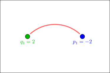
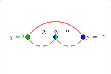
Figure 1: Distances between two sets $s,s^{\prime}$, each of which contains one particle (left panel) or two particles (right panel). Blue dots represent particles in set $s$, green dots stand for particles in set $s^{\prime}$. The possible pairings used in the distance calculation are indicated by lines. The square norm $d^{2}$ erroneously results in a shorter distance for the pairing indicated by the dashed line.

2.1.3 Example for an Event Distance

To illustrate one possible distance measure, let us consider a simple yet non-trivial example, where we calculate the distance between two events $e$ and $e^{\prime}$. $e$ has two outgoing photons and a jet, and $e^{\prime}$ two photons and no jets. The distance between the two events is therefore

$$d(e,e^{\prime})=d(s_{\gamma},s_{\gamma}^{\prime})+d(s_{j},s_{j}^{\prime}).$$ (18)

The jet set $s_{j}$ for the event $e$ contains a single jet with momentum $p_{j}$, whereas the corresponding set $s_{j}^{\prime}$ for $e^{\prime}$ is empty. Likewise, $s_{\gamma}$ contains the photons in $e$ with momenta $p_{1},p_{2}$ and $s_{\gamma}^{\prime}$ the photons in $e^{\prime}$ with momenta $p_{1}^{\prime},p_{2}^{\prime}$. The distance between these two sets is

$$d(s_{\gamma},s_{\gamma}^{\prime})=\min\Bigl{[}d(p_{1},p_{1}^{\prime})+d(p_{2},p_{2}^{\prime}),d(p_{1},p_{2}^{\prime})+d(p_{2},p_{1}^{\prime})\Bigr{]},$$ (19)

where $d(p,q)=\sqrt{\sum_{i=1}^{3}(p_{i}-q_{i})^{2}+\tau^{2}(p_{\perp}-q_{\perp})^{2}}$ is the distance introduced in equation (13).

To calculate the distance $d(s_{j},s_{j}^{\prime})$ between the jet sets, we first add an auxiliary “jet” with vanishing momentum $p_{j}^{\prime}=0$ to $s_{j}^{\prime}$, so that both sets each contain a single jet. The set distance is then

$$d(s_{j},s_{j}^{\prime})=d(p_{j},p_{j}^{\prime})=\sqrt{\sum_{i=1}^{3}p_{ji}^{2}+\tau^{2}p_{j\perp}^{2}},$$ (20)

where $p_{j}$ denotes the momentum of the physical jet.

2.1.4 Distances in high-dimensional spaces

When considering a fixed number of generated events in phase spaces of increasing dimension, the typical distance between two events, and therefore the characteristic cell size, will grow very quickly. Conversely, when trying to achieve a given cell size, the required number of events will become prohibitively large very soon. We might be worried that for processes with many final-state particles cells unavoidably become so large that they can be resolved experimentally. This is not the case. The reason is that experimental resolution is limited by statistics in addition to detector limitations. In fact, the sizes of resolved regions of phase space will increase in the same way as the cell sizes with the number of dimensions.

It is instructive to consider how the final cell size in a high-dimensional phase space translates to differences in real-world observables, which are typically low-dimensional distributions. To obtain some quantitative insight, we can model a cell as an $n$-ball with radius $R$ in a $n$-dimensional Euclidean space. For a sufficiently small radius, events within the cell will be approximately uniformly distributed. The exceptions are the cell seed at the centre and the last event added at a distance $R$ to the cell. It is well known that for large $n$, events tend to be close to the surface, and the mean distance of an event to the seed is indeed given by

$$\bar{d}=\frac{1}{V_{n}}\int dV_{n}\ r=\frac{n}{n+1}R,$$ (21)

where $V_{n}$ is the volume of the $n$-ball. However, when predicting one-dimensional distributions, we project the events onto a line, which we can take as the $n$-th coordinate axis. For the mean distance in this direction we obtain

$$\bar{d}_{n}=\frac{1}{V_{n}}\int dV_{n}\ r_{n}=\frac{\Gamma(\frac{n}{2}+1)}{\Gamma(\frac{1}{2})\Gamma(\frac{n+3}{2})}R=\mathcal{O}\left(\frac{1}{\sqrt{n}}\right).$$ (22)

The difference in one-dimensional distributions is much smaller than the cell size, especially in high-dimensional phase spaces.

2.2 Nearest-Neighbour Search and Locality-Sensitive Hashing

A very appealing feature of cell resampling is that the cell radii automatically become smaller with increasing number of events. Anticipating the discussion of the practical application with the distance measure in section 3, we indeed find a significant reduction in cell size, as shown in figure 2. Due to large fluctuations in the weights of the cell seeds, and correspondingly in the cell sizes, we consider the median of the cell radii instead of the arithmetic mean.

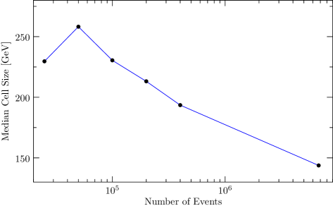
Figure 2: Median cell radius as a function of sample size according to the distance measure defined in section 2.1.1 with $\tau=0$. See section 3 for details on the event generation.

From this point of view, cell resampling should be applied to event samples that are as large as possible. However, the main motivation behind the resampling is to reduce the computational cost of later steps. This implies that the CPU time needed for resampling should be much smaller. On the one side, various event generation steps are usually performed on an event-by-event basis, and the asymptotic generation time scales linearly with the number $n$ of events. On the other side, the number of negative-weight events and therefore the number of cells are also proportional to $n$. To achieve the same asymptotic $\mathcal{O}(n)$ runtime scaling, the time to construct a single cell has to be constant, i.e. independent of the sample size. However, while obviously asymptotically inferior, overall $\mathcal{O}(n\log^{k}n)$ scaling for some integer $k$ will presumably be sufficient for real-world sample sizes.

To reiterate, a cell is constructed as follows. We choose a seed, i.e. one of the remaining negative-weight events. As long as the sum of weights inside the cell is negative, we subsequently find the closest event to the seed outside the cell according to our distance function and add it to the cell. Finally, we reweight all events inside the cell.

The selection of a negative-weight event can be achieved in constant time with the help of a pregenerated array containing these events, which can be created in $\mathcal{O}(n)$ steps. If we want to construct cells in a specific order, an additional $\mathcal{O}(n\log n)$ sorting step is required. The impact of different seed selection strategies is discussed in appendix A.

The biggest challenge is to find nearby events in constant or, at worst, logarithmic time. A naive nearest-neighbour search requires $\mathcal{O}(n)$ operations for each cell, leading to an overall $\mathcal{O}(n^{2})$ scaling. Nearest-neighbour search is a well-studied problem in computer science. In modern particle physics, one of the most prominent applications is jet clustering Cacciari:2005hq . However, jet clustering requires searches in two dimensions and the algorithms used there are not suited for the present high-dimensional problem. For approximate searches in high-dimensional spaces, locality-sensitive hashing (LSH) Indyk1998 ; Leskovec:2020 has been found to be highly efficient. In the following we give a short outline while describing one way in which LSH can be used for finding events that are close to a given cell.

First, we relax the condition that cells have to be kept spherical by subsequently adding nearest neighbours. We will contend ourselves with cells that are small in each phase-space direction and, most importantly, shrink with increasing statistics. This can be achieved by an approximate nearest-neighbour search.

In order to being able to apply standard techniques, we map the events onto points in a high-dimensional Euclidean space. A crucial observation is that this map does not have to preserve distances, neither in the absolute nor in the relative sense. It is sufficient that events that are nearby in phase space are mapped onto points that are nearby in Euclidean space with high probability. To this end, we recall that, in each event $e$, we group particles into sets $s_{e,t}$ according to their type $t$. To each of these sets, we now add particles with vanishing four-momentum until for each particle type all sets in all events have the same number of elements, i.e.

$$|s_{e,t}|=|s_{e^{\prime},t}|\qquad\text{for all events }e,e^{\prime}\text{ and types }t\,.$$ (23)

We then interpret each set $s_{e,t}$ as a tuple $\tau_{e,t}=\big{(}p_{e,t,1},\dots,p_{e,t,P_{t}}\big{)}$ of $P_{t}$ four-momenta, which we sort lexicographically according to the momentum components. Finally, for the event $e$ the coordinates of the resulting point $V_{e}$ in Euclidean space correspond to the spatial momentum components in order. The first three components $i=1,2,3$ are obtained from the first spatial momentum in the tuple for the first particle type, i.e. $(V_{e})_{i}=(p_{e,1,1})_{i}$. The next three components correspond to the second momentum in the tuple for the first particle type, and after reaching the last momentum in a tuple we proceed to the tuple for the next particle type. The total dimension of the Euclidean space is therefore

$$D=3\sum_{t=1}^{T}|s_{e,t}|\,,$$ (24)

which is independent of the chosen event $e$. Events $e$ and $e^{\prime}$ which are nearby in phase space will most likely have a similar number of outgoing particles of each type with similar momenta. Therefore, the coordinates of $V_{e}$ and $V_{e^{\prime}}$ will be similar and the points will be close to each other.

We have now recast the problem to finding approximate nearest neighbours between the points $V_{e}$ in a $D$-dimensional Euclidean space. To facilitate this task, we consider random projections onto lower dimensional sub spaces. This is a well-established technique motivated by the Johnson-Lindenstrauss Lemma JohnsonLindenstrauss , which states that it is always possible to find projections that nearly preserve the distances between the points. Specifically, we define projections $\Pi_{h}$ onto hyperplanes $h=1,\dots,H$, each fixed by a randomly chosen unit normal vector as discussed in Muller:1959 ; Marsaglia:1972 . $H$ should be chosen in such a way that it grows logarithmically with the number of points, i.e. the number of events. We then perform a second projection onto the $x$ axis, i.e. we take the first coordinate of each projected vector:

$$V_{e}\mapsto c_{e,h}=\left(\Pi_{h}V_{e}\right)_{1}.$$ (25)

For each $h=1,\dots,H$, we sort the coordinates $c_{e,h}$ obtained from all events $e$ in the sample and divide them into buckets of size $B$. $B$ may increase at worst logarithmically with the number of events, otherwise the described algorithm for cell creation would no longer fulfil our time complexity constraint, as shown later. Note that events $e,e^{\prime}$ with nearby coordinates $c_{e,h},c_{e^{\prime},h}$ will be inside the same bucket with high probability.

This effectively defines $H$ hash functions $f_{h}$, each of which maps a given event onto a single integer number, namely the index of the bucket associated with the coordinate $c_{e,h}$:

$$f_{h}:\qquad e\mapsto\operatorname{bucket}\left[c_{e,h}\right]=\operatorname{bucket}\left[\left(\Pi_{h}V_{e}\right)_{1}\right]\,.$$ (26)

These hash functions are locality sensitive. Nearby events are likely to be mapped onto the same number.

We use the hash functions to create $H$ hash tables, where we store the values of $f_{h}(e)$ for all events $e$. When creating a cell, we look up the hashed values $f_{h}(e)$ for the seed event $e$. We then consider all events that lie in the same bucket as $e$ in one of the $H$ projected coordinates, i.e. at most $HB$ events. In practice, the number will be much lower, as nearby events will share more than one bucket with $e$. Starting from the events sharing the most buckets with $e$, we identify nearest neighbour candidates. We select candidates with weights $w_{i}$, until we fulfil

$$\sum_{i}w_{i}\geq-aw_{e}\,,$$ (27)

where $w_{e}$ is the (negative) seed weight and $a$ an arbitrary constant with $a\geq 1$. In our implementation, we choose $a=2$.

For each of the nearest neighbour candidate, we then compute the actual distance to the seed $e$ using the metric defined in section 2.1. We proceed to add nearest neighbours according to the actual distance to the cell, as we did when using naive nearest-neighbour search, until the sum of weights inside the cell is no longer negative.

Let us now analyse the asymptotic time complexity of the LSH-based algorithm. To create the hash table, we have to compute $H$ projected coordinates for each of the $n$ events, where $H=\mathcal{O}(\log n)$. Once the $H$ hyperplanes are fixed, each coordinate can be computed independently in constant time. In total we compute $\mathcal{O}(Hn)=\mathcal{O}(n\log n)$ coordinates. For each $h$, we have to sort the coordinates of $n$ events, which gives a time complexity of $\mathcal{O}(Hn\log n)=\mathcal{O}(n\log^{2}n)$. The partitioning into buckets is again linear in the number of events, and therefore asymptotically negligible compared to the sorting.

Looking up the values of the hash functions for a single seed event requires $\mathcal{O}(H)=\mathcal{O}(\log n)$ operations. To select the candidates we have to probe all events in $H$ buckets of size $B$, with time complexity $\mathcal{O}(HB)=\mathcal{O}(\log^{2}n)$. Since the number of events needed to compensate the seed weight does not increase with $n$, only a constant number of distance functions have to be calculated after selecting candidates. In total, the number of cells grows linearly with $n$ and the creation of each cell requires $\mathcal{O}(\log^{2}n)$ constant-time steps, which results in an overall time complexity of $\mathcal{O}(n\log^{2}n)$.

Finally, we consider the practical performance of our implementation for various sample sizes. Figure 3 compares the median cell size, measured by the largest distance between the seed and any other event inside the cell, and scaling of the computing time to the naive linear nearest-neighbour search. Heuristically, we have chosen $H=15\log n$ hash functions and a fixed bucket size of $B=1000$. We find that the required computing time indeed scales much better with increased sample size. However, the cell size does not seem to decrease significantly with larger statistics. We conclude that further improvements are needed to render the LSH-based approach competitive compared to the linear nearest-neighbour search.

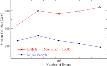
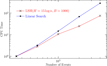
Figure 3: Comparison between linear nearest-neighbour search and the LSH-based approach with $H=15\log n$ hash functions and buckets containing $B=1000$ events. The left panel shows the median cell size as a function of the number of input events. The right panel illustrates the scaling of the computing time with the sample size. The respective timings are normalised to the first data point in order to facilitate comparison and eliminate constant factors resulting from differences in the implementation.

2.3 Relation to Positive Resampling

Let us comment on the relation between the current approach and the positive resampler suggested in Andersen:2020sjs . There, events are collected in histogram bins and positive resampling, i.e. replacing event weights by rescaled absolute values, is performed on each bin separately.

There is a clear parallel to the LSH-based method presented in section 2.2. Where the LSH includes random projections of events onto coordinates, positive resampling projects events onto one or more observables defined by the chosen histogram, such as particle transverse momenta. The histogram bins then correspond to the buckets in the locality-sensitive hash tables. Following the same philosophy behind the random projection method, we expect events in the same histogram bins to be also close in other phase-space directions with high probability.

Positive resampling as presented in Andersen:2020sjs is therefore similar to cell resampling with LHS-based nearest-neighbour search with a small number of $H\leq 3$ hash functions. An important difference is the definition of a cell. The equivalent for the positive resampler would be an entire bin, i.e a complete hash bucket. For this reason, it is difficult to perform a rigorous direct comparison between the two approaches. However, we can get an idea by comparing cell resampling with linear nearest-neighbour search and LSH-based search with small $H$. In figure 4 we compare the median cell sizes obtained in both approaches for different sample sizes. We have increased the bucket size to $B=20000$ to ensure that sufficiently many nearest-neighbour candidates are found.

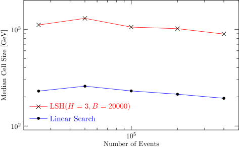
Figure 4: Comparison of the median cell size between linear nearest-neighbour search and the LSH-based approach with three hash functions.

3 Cell Resampling for the Production of a W Boson with two Jets

We now demonstrate the proposed method through a highly non-trivial application. We consider the production of a leptonically decaying W^- boson together with at least two jets in proton-proton collisions at 7 TeV centre-of-mass energy calculated at next-to-leading order. Weighted events are generated using Sherpa Bothmann:2019yzt with OpenLoops Buccioni:2019sur . Generation parameters are shown in table 1.

# events	$6.1\times 10^{7}$	(low-statistics input sample)
	$1.5\times 10^{10}$	(high-statistics reference sample)
$\mu_{r},\mu_{f}$	$\frac{H_{T}}{2}$
$\sqrt{s}$	7 TeV
PDF	NNPDF 3.1 NNPDF:2017mvq ; Buckley:2014ana
Jet definition	anti-$k_{t}$ Cacciari:2008gp
	$R=0.4$
	$p_{\perp}>30\,$GeV
	$|\eta|<4.4$
$m_{W}$	80.385 GeV
$\Gamma_{W}$	2.085 GeV
$1/\alpha_{\text{QED}}(0)$	132.232

Table 1: Parameters used for event generation.

The 2-parton samples receive contributions from Born, virtual, and subtraction terms, and the 3-parton samples from subtraction and real emission. The sum should be positive, provided reasonable choices for the renormalisation and factorisation scales have been applied. We choose $\mu_{f}=\mu_{r}=H_{T}/2$. The subtraction terms can extend far in phase space, which can cause non-local bin-to-bin migration in an analysis of distributions, and issues for the current resampling based on phase space buckets. This issue can be reduced by applying the modified subtractions Nagy:2001fj ; Nagy:2003tz to restrict their size. We have not done so in the current study, partly to illustrate the performance of the resampler in a “worst case” scenario.

To assess the performance of our method, we use $6.1\times 10^{7}$ events as input and compare both this original NLO sample and the output of the cell resampler to a reference prediction obtained from a high-statistics sample with $1.5\times 10^{10}$ events. For the cell resampling, we choose the distance measure introduced in section 2.1.1, and determine the contribution from transverse momentum differences by setting the parameter $\tau$ to 10, c.f. equation (13). Since the computing time required for cell resampling grows quadratically with the number of events, we split the input sample into nine samples of equal size and apply the resampling separately to each of them. At the same time, we impose an upper limit for the cell radius of 100 GeV in order to achieve cell sizes commensurate with the combined sample size. While this limit prevents us from eliminating all negative event weights, it still reduces their overall contribution by more than an order of magnitude. This is illustrated in figure 5.

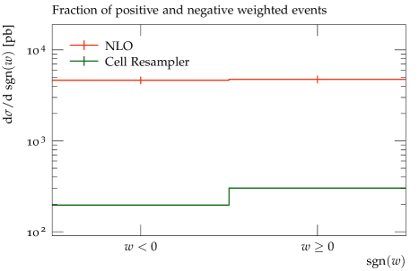
Figure 5: Contributions of negative- and positive-weight events to the cross section according to the MC_XS Rivet analysis.

The NLO calculation achieves a $\sim 10^{2}\,$pb cross section as cancellation between terms of size $\sim 5\times 10^{3}\,$pb, whereas the cell resampler obtains the same cross section as a difference between terms of $\sim 3\times 10^{2}\,$pb and $\sim 2\times 10^{2}\,$pb. If we were to reweight the events to weight $\pm 1$, the original NLO sample would result in almost $20$ times as many events compared to unweighting the resampled events. This corresponds to a Monte Carlo estimate of the uncertainty which is larger by a factor of approximately $\sim\sqrt{20}$. Conversely, to achieve the same estimated uncertainty as reached after resampling, a pure NLO sample would require the generation of almost 20 times as many events.

The events are parsed through the standard Rivet Bierlich:2019rhm analyses MC_XS and MC_WJETS, plus a relevant ATLAS analysis ATLAS:2014fjg in order to demonstrate the performance for calculations relevant for experimental measurements. As the point of this study is not to compare with experimental data, but to improve on the stability of the predictions, we will for simplicity use the calculation of just $pp\to e^{-}\bar{\nu}_{e}jj$ and not the positron channel. In addition, we also extract the rapidity distribution of the W boson using a custom analysis based on the Rivet framework.

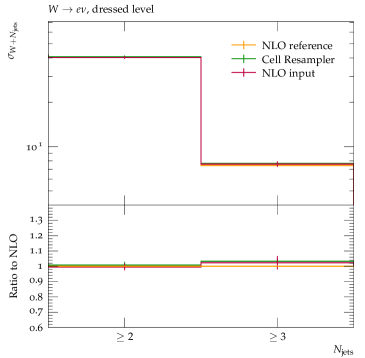
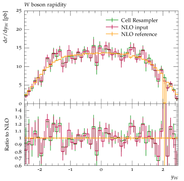
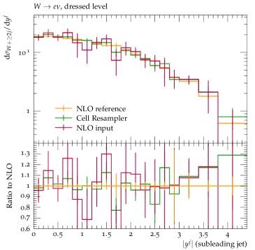
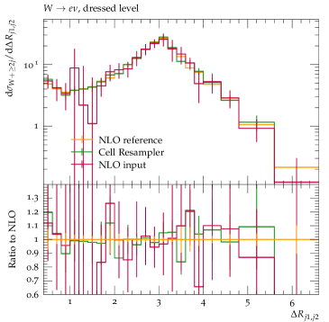
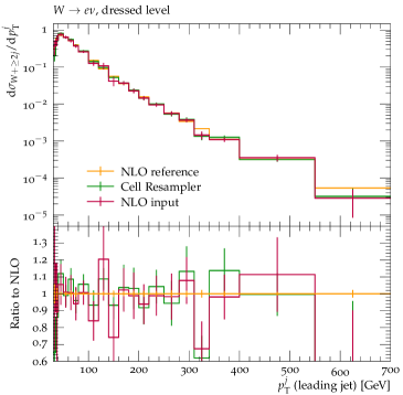
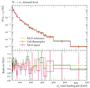
Figure 6: The results from the pure NLO calculation and of resampler for a subset of the analyses performed. See text for further details.

Figure 6 compares the vanilla prediction for the NLO calculation and the result of passing the low-statistics NLO event sample through the resampler for several observables. The results for the inclusive two and three jet cross sections are shown in the top left plot. Both the low-statistics NLO result and that of the cell resampler are stable, as expected. The vertical lines indicate the statistical uncertainty estimated from the weight distribution interpreted as a Monte Carlo sample. The estimate of the uncertainty is larger from the pure NLO sample than that of the cell resampler, simply because of the reduction in the variance of the weights in the event sample.

Having demonstrated that the predictions for inclusive two and three jet production are preserved by the cell resampling, we now consider differential distributions. The top right plot of figure 6 shows the rapidity distribution of the W boson. The level of agreement with the reference prediction within the Monte Carlo error estimate is similar between the original low-statistics NLO sample and the cell resampler. Concretely, the $\chi^{2}$ per degree of freedom is $1.18$ for the cell resampler and $1.25$ for the low-statistics NLO sample when comparing to the reference distribution. We conclude that the nominal reduction of the statistical uncertainty through cell resampling is indeed accompanied by a stabilisation of the predicted distributions. Furthermore, the Monte Carlo estimate of the uncertainty in each bin correlates well with the statistical jitter between bins.

It is important to note here that contrary to the approach in Andersen:2020sjs , there is no input to the cell resampler about any analyses intended for the sample. This implies that the observed good agreement with the high-statistics reference predictions would not be limited to the rapidity distribution of the W boson. Indeed, the plots on the middle row of figure 6 show that the reference prediction is also matched well in the distribution in the absolute rapidity of the hardest jet, $|y_{j_{1}}|$ and $\Delta R_{{j_{1}},{j_{2}}}$, both calculated according to the analysis in ATLAS:2014fjg .

Finally, the bottom row in figure 6 shows the distributions on the transverse momentum of the hardest and second hardest jet. These distributions are significantly smoother straight from the NLO calculation. They are smoother still from the cell resampler. At the same time, the cells appear to be sufficiently small, such that neither these steeply falling distributions nor the peak in the $\Delta R_{{j_{1}},{j_{2}}}$ distribution are smeared out to any visible degree.

4 Conclusions

We have presented cell resampling as a method to eliminate negative event weights. Negative weights are redistributed locally in phase space and any potential bias introduced by this redistribution becomes arbitrarily small given sufficient statistics.

We have demonstrated the real-world performance on the highly non-trivial example of the production of a W boson with two jets at NLO. It is straightforward to apply our method to arbitrary processes, and we provide an easy-to-use implementation available from https://cres.hepforge.org/ to this end.

A central ingredient of cell resampling is the definition of a distance function between events in phase space. This function should mirror experimental sensitivity without referring to any specific analysis. We have proposed a simple metric, which is shown to perform well in practice. The exploration of more sophisticated distance functions is a promising avenue towards future improvements of the cell resampling method.

Since the quality of the reweighted event samples increases systematically with their size, it is important that the computational cost of cell resampling scales well with the number of input events. To achieve this, we have explored an algorithm for nearest-neighbour search in phase space based on random projections and locality-sensitive hashing. While we find a significantly improved scaling behaviour compared to naive linear search, further improvements will be necessary to obtain the same increase in quality with growing statistics.

Appendix A Seed selection strategies

When introducing cell resampling in section 2, the only criterion for picking a cell seed was that the event weight has to be negative. We may wonder whether constructing cells in a specific order changes the final result. To answer this question, we assess three different strategies for selecting the seed for the next cell.

1. Choose the event with the most negative weight (“most negative”).

2. Choose the next negative-weight event according to the order in which events were generated (“in order”).

3. Choose the negative-weight event with weight closest to zero (“least negative”).

We are primarily interested in the quality of the outcome, i.e. the resampling should affect observables as little as possible. As a proxy for this very general requirement, we first consider the cell size distributions. After quality, a secondary criterion is speed. In figure 7, we compare the median cell sizes as a function of computing time for samples with between 25 and 400 thousand events. We also show the distribution of cell radii for the largest event sample.

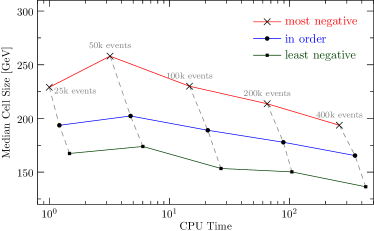
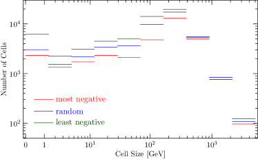
Figure 7: Comparison of different strategies for selecting cell seeds. On the left, we show the median cell radius as a function of computing time. Timings are normalised to the fastest run with $25\,000$ events and the “most negative” strategy. On the right, we show the distribution of cell radii for the sample with $400\,000$ events.

We might be tempted to conclude that the “least negative” strategy is best: despite being the slowest for any given sample, it consistently produces smaller cells given either a fixed number of input events or even a fixed computing time budget. However, we also notice that this strategy not only produces more small-sized cells, but also a larger number of big cells. By choosing seeds with weight close to zero first, we tend to construct cells with increasing radii. Cells that are constructed early on may easily be subsumed by later cells, which implies that the time spend on constructing the earlier cell is wasted and the median cell size is no longer a good indicator of quality.

We can limit the impact of big cells by imposing a maximum cell radius. In this case, we can measure the quality of the resampling through the negative-weight factor

$$\hat{\sigma}_{-}=\frac{1}{\sigma}\frac{d\sigma}{d\operatorname{sgn}w}\bigg{|}_{w=-1}=-\frac{\sum_{w_{i}<0}w_{i}}{\sum_{i}w_{i}},$$ (28)

where $w_{i}$ is the weight of event $i$. For the initial event sample with $400\,000$ events we find $\hat{\sigma}_{-}\approx 26.1$. Resampling with a maximum cell radius of $100\,$GeV yields $\hat{\sigma}_{-}\approx 1.1$, with fluctuations at the level of one per cent between the different strategies. We do not observe any significant differences in run time.

In conclusion, we propose the following modus operandi. First, we estimate the typical cell size through test runs without imposing any limit on the radius. To save computing time we can employ the “most negative” strategy and extrapolate from smaller event samples. We then perform the actual resampling with a cell radius limit of the order of the estimated median. Following the above discussion, we do not expect any significant dependence of the final results on the cell selection strategy.

References

- (1) S. Catani and M. H. Seymour, A General algorithm for calculating jet cross-sections in NLO QCD, Nucl. Phys. B 485 (1997) 291–419, [hep-ph/9605323].
- (2) S. Catani, S. Dittmaier, M. H. Seymour and Z. Trocsanyi, The Dipole formalism for next-to-leading order QCD calculations with massive partons, Nucl. Phys. B 627 (2002) 189–265, [hep-ph/0201036].
- (3) S. Frixione and B. R. Webber, Matching NLO QCD computations and parton shower simulations, JHEP 06 (2002) 029, [hep-ph/0204244].
- (4) P. Nason and G. Ridolfi, A Positive-weight next-to-leading-order Monte Carlo for Z pair hadroproduction, JHEP 08 (2006) 077, [hep-ph/0606275].
- (5) J. C. Collins, D. E. Soper and G. F. Sterman, Transverse Momentum Distribution in Drell-Yan Pair and W and Z Boson Production, Nucl. Phys. B 250 (1985) 199–224.
- (6) V. S. Fadin, E. Kuraev and L. Lipatov, On the Pomeranchuk Singularity in Asymptotically Free Theories, Phys. Lett. B 60 (1975) 50–52.
- (7) I. I. Balitsky and L. N. Lipatov, The Pomeranchuk singularity in quantum chromodynamics, Sov. J. Nucl. Phys. 28 (1978) 822–829.
- (8) S. Höche, F. Krauss, M. Schönherr and F. Siegert, QCD matrix elements + parton showers: The NLO case, JHEP 04 (2013) 027, [1207.5030].
- (9) L. Lönnblad and S. Prestel, Merging Multi-leg NLO Matrix Elements with Parton Showers, JHEP 03 (2013) 166, [1211.7278].
- (10) L. Lönnblad and S. Prestel, Unitarising Matrix Element + Parton Shower merging, JHEP 02 (2013) 094, [1211.4827].
- (11) GEANT4 collaboration, S. Agostinelli et al., GEANT4–a simulation toolkit, Nucl. Instrum. Meth. A 506 (2003) 250–303.
- (12) J. Alwall, R. Frederix, S. Frixione, V. Hirschi, F. Maltoni, O. Mattelaer et al., The automated computation of tree-level and next-to-leading order differential cross sections, and their matching to parton shower simulations, JHEP 07 (2014) 079, [1405.0301].
- (13) J. Bellm et al., Herwig 7.0/Herwig++ 3.0 release note, Eur. Phys. J. C76 (2016) 196, [1512.01178].
- (14) T. Sjöstrand, S. Ask, J. R. Christiansen, R. Corke, N. Desai, P. Ilten et al., An Introduction to PYTHIA 8.2, Comput. Phys. Commun. 191 (2015) 159–177, [1410.3012].
- (15) Sherpa collaboration, E. Bothmann et al., Event Generation with Sherpa 2.2, SciPost Phys. 7 (2019) 034, [1905.09127].
- (16) K. Danziger, S. Höche and F. Siegert, Reducing negative weights in Monte Carlo event generation with Sherpa, 2110.15211.
- (17) R. Frederix, S. Frixione, S. Prestel and P. Torrielli, On the reduction of negative weights in MC@NLO-type matching procedures, 2002.12716.
- (18) C. Gao, J. Isaacson and C. Krause, i-flow: High-dimensional Integration and Sampling with Normalizing Flows, Mach. Learn. Sci. Tech. 1 (2020) 045023, [2001.05486].
- (19) E. Bothmann, T. Janßen, M. Knobbe, T. Schmale and S. Schumann, Exploring phase space with Neural Importance Sampling, SciPost Phys. 8 (2020) 069, [2001.05478].
- (20) C. Gao, S. Höche, J. Isaacson, C. Krause and H. Schulz, Event Generation with Normalizing Flows, Phys. Rev. D 101 (2020) 076002, [2001.10028].
- (21) J. R. Andersen, C. Gütschow, A. Maier and S. Prestel, A Positive Resampler for Monte Carlo events with negative weights, Eur. Phys. J. C 80 (2020) 1007, [2005.09375].
- (22) B. Nachman and J. Thaler, Neural resampler for Monte Carlo reweighting with preserved uncertainties, Phys. Rev. D 102 (2020) 076004, [2007.11586].
- (23) B. Stienen and R. Verheyen, Phase Space Sampling and Inference from Weighted Events with Autoregressive Flows, 2011.13445.
- (24) P. T. Komiske, E. M. Metodiev and J. Thaler, Metric Space of Collider Events, Phys. Rev. Lett. 123 (2019) 041801, [1902.02346].
- (25) M. Crispim Romão, N. F. Castro, J. G. Milhano, R. Pedro and T. Vale, Use of a generalized energy Mover’s distance in the search for rare phenomena at colliders, Eur. Phys. J. C 81 (2021) 192, [2004.09360].
- (26) M. Cacciari and G. P. Salam, Dispelling the myth for the jet-finder, Phys. Lett. B 641 (2006) 57–61, [hep-ph/0512210].
- (27) P. Indyk and R. Motwani, Approximate nearest neighbors: Towards removing the curse of dimensionality, in Proceedings of the 30th ACM Symposium on Theory of Computing, p. 604–613, 1998.
- (28) J. Leskovec, A. Rajaraman and J. Ullman, Mining of Massive Datasets. Cambridge University Press, 2020.
- (29) W. B. Johnson and J. Lindenstrauss, Extensions of Lipschitz mappings into a Hilbert space, Contemp. Math. (1984) 189–206.
- (30) M. E. Muller, A Note on a Method for Generating Points Uniformly on N-Dimensional Spheres, Comm. Assoc. Comput. Mach. 2 (1959) 19–20.
- (31) G. Marsaglia, Choosing a Point from the Surface of a Sphere, Ann. Math. Stat. 43 (1972) 645–646.
- (32) F. Buccioni, J.-N. Lang, J. M. Lindert, P. Maierhöfer, S. Pozzorini, H. Zhang et al., OpenLoops 2, Eur. Phys. J. C 79 (2019) 866, [1907.13071].
- (33) NNPDF collaboration, R. D. Ball et al., Parton distributions from high-precision collider data, Eur. Phys. J. C 77 (2017) 663, [1706.00428].
- (34) A. Buckley, J. Ferrando, S. Lloyd, K. Nordström, B. Page, M. Rüfenacht et al., LHAPDF6: parton density access in the LHC precision era, Eur. Phys. J. C 75 (2015) 132, [1412.7420].
- (35) M. Cacciari, G. P. Salam and G. Soyez, The anti- jet clustering algorithm, JHEP 04 (2008) 063, [0802.1189].
- (36) Z. Nagy, Three jet cross-sections in hadron hadron collisions at next-to-leading order, Phys. Rev. Lett. 88 (2002) 122003, [hep-ph/0110315].
- (37) Z. Nagy, Next-to-leading order calculation of three jet observables in hadron hadron collision, Phys. Rev. D 68 (2003) 094002, [hep-ph/0307268].
- (38) C. Bierlich et al., Robust Independent Validation of Experiment and Theory: Rivet version 3, SciPost Phys. 8 (2020) 026, [1912.05451].
- (39) ATLAS collaboration, G. Aad et al., Measurements of the W production cross sections in association with jets with the ATLAS detector, Eur. Phys. J. C 75 (2015) 82, [1409.8639].