Frequent Itemset Mining with Multiple Minimum Supports: a Constraint-based Approach

Abstract

The problem of discovering frequent itemsets including rare ones has received a great deal of attention. The mining process needs to be flexible enough to extract frequent and rare regularities at once. On the other hand, it has recently been shown that constraint programming is a flexible way to tackle data mining tasks. In this paper, we propose a constraint programming approach for mining itemsets with multiple minimum supports. Our approach provides the user with the possibility to express any kind of constraints on the minimum item supports. An experimental analysis shows the practical effectiveness of our approach compared to the state of the art.

1 Introduction

Discovering relevant patterns for a particular user remains a challenging task in data mining. In real-life applications, relevant patterns may be either frequent or rare ones in the data. In itemset mining, setting the minimum support threshold is a real dilemma (a high value misses rare itemsets, a low value generates a large number of meaningless itemsets). To tackle the rare item problem [8], several approaches were proposed to mine frequent pattern with multiple minimum supports. In [8], the problem of mining frequent itemsets with multiple Minimum Item Supports (MIS) was introduced with a first revision of Apriori algorithm (${\tt MSApriori}$). Then, other Apriori-like approaches were proposed like ${\tt MMS\_Cumulate}$ and ${\tt MMS\_Stratify}$ [12]. The well-known ${\tt FPGrowth}$ was extended with a condensed FP-tree structure to mine frequent itemsets with multiple MIS (${\tt CFPGrowth}$ [5], ${\tt CFPGrowth++}$ [6]). In [3], ${\tt FP-ME}$ was proposed based on set-enumeration-tree structure and sorted downward closure property.

The specialized algorithms introduced previously are effective for mining patterns with multiple MIS. However, most of the time the user is interested in patterns that satisfy some specific properties. For instance, the user may ask for patterns where items are around the same frequency threshold, or patterns of an adaptive size (large frequent patterns and/or concise rare patterns). Looking for patterns with additional user-specified constraints remains a bottleneck. According to Wojciechowski and Zakrzewicz [13], there are three ways to handle the additional user’s constraints. We can use a pre-processing step that restricts the dataset to only transactions that satisfy the constraints. Such a technique cannot be used on all kinds of constraints. We can use a post-processing step to filter out the patterns violating the user’s constraints. Such a brute-force technique can be computationally infeasible when the problem without the user’s constraints has too many solutions. We can finally integrate the filtering of the user’s constraints into the specialized data mining process in order to extract only the patterns satisfying the constraints. Such a technique requires the development of a new algorithm for each new mining problem with user’s constraints.

In a recent line of work [9, 7, 11, 1, 2], constraint programming (CP) has been used as a declarative way to solve some data mining tasks. Such an approach has not competed yet with state of the art data mining algorithms in terms of CPU time for standard data mining queries but the CP approach is competitive as soon as we need to add user’s constraints. In addition, adding constraints is easily done by specifying the constraints directly in the model without the need to revise the solving process. However, the CP approach has not yet been applied to mining frequent itemsets with multiple MIS.

In this paper we introduce a CP model for finding frequent itemsets with multiple MIS. For that, we introduce a new global constraint, FreqRare for mining frequent itemsets with multiple MIS. We provide a propagator for FreqRare and we show that, for a given variable ordering, it is sufficient to mine frequent itemsets with multiple MIS in backtrack-free manner. Our constraint, FreqRare, can be used to express any kind of constraints on the minimum item supports. We show that our CP model can easily be extended for taking into account any kind of user’s constraints. Experiments on several known large-scale datasets show the effectiveness of our CP model.

The paper is organized as follows. Section 2 gives some background material. Section 3 presents our global constraint FreqRare and its propagator. Section 4 presents the possible extensions of our CP model to express constraints on the minimum item supports. Section 5 reports experiments. Finally, we conclude in Section 6.

2 Background

2.1 Itemset mining

Let $\mathcal{I}=\{p_{1},\ldots,p_{n}\}$ be a set of $n$ distinct objects, called items. An itemset $P$ is a non-empty subset of $\mathcal{I}$. A transactional dataset $\mathcal{D}$ is a bag of $m$ itemsets $t_{1},\ldots,t_{m}$, called transactions. The cover of an itemset $P$ in $\mathcal{D}$, denoted by $cover(P)$, is the bag of transactions from $\mathcal{D}$ containing $P$.

The frequency of an itemset $P$ in $\mathcal{D}$, denoted by $freq(P)$, is the cardinality of its cover, i.e. $freq(P)=|cover(P)|$. Let $\mathcal{S}=\{s_{1},\ldots,s_{n}\}$ be a set of minimum supports associated to items (i.e., the multiple MIS set), where $s_{i}$ is the minimum support of the item $p_{i}$. The itemset $P$ is frequent iff:

$$freq(P)\geq\min\limits_{p_{i}\in P}s_{i}$$

For the sake of simplicity, we replace in what follows items $p_{i}$ and transactions $t_{j}$ with their respective indices $i$ and $j$ and we denote the presence of item $i$ in transaction $j$ by $\mathcal{D}_{ij}$.

Example 2.1

The $D$ dataset presented in Table 1 has $4$ items and $5$ transactions. According to its multiple MIS, $AB$ is frequent, $ABC$ is infrequent and $ABCD$ is frequent.

Table 1: Transaction dataset example $D$ with its corresponding MIS set $S$.

$D$: trans. Items $t_{1}$ $A$ $B$ $D$ $t_{2}$ $A$ $C$ $D$ $t_{3}$ $A$ $B$ $C$ $D$ $t_{4}$ $B$ $C$ $t_{5}$ $A$ $B$ $C$     $S:$ $A$ $B$ $C$ $D$ 4 3 3 1

2.2 Constraint programming

A Constraint Programming model (or CP model) specifies a set of variables $X=\{x_{1},\ldots,x_{n}\}$, a set of domains $dom=\{dom(x_{1}),\ldots,dom(x_{n})\}$, where $dom(x_{i})$ is the finite set of possible values for $x_{i}$, and a set of constraints $\mathcal{C}$ on $X$. A constraint $c_{j}\in\mathcal{C}$ is a relation that specifies the allowed combinations of values for its variables $var(c_{j})$. An assignment on a set $Y\subseteq X$ of variables is a mapping from variables in $Y$ to values, and a valid assignment is an assignment where all values belong to the domain of their variable. A solution is an assignment on $X$ satisfying all constraints. Constraint programming is the art of writing problems as CP models and solving them by finding solutions. Constraint solvers typically use backtracking search to explore the search space of partial assignments. At each assignment, constraint propagation algorithms (aka, propagators) prune the search space by enforcing local consistency properties such as domain consistency.

Global constraints are constraints defined by a relation on a non-fixed number of variables. These constraints allow the solver to better capture the structure of the problem. The constraint AllDifferent, specifying that all its variables must take different values is an example of global constraint (see [10]).

Example 2.2

Consider the following instance of a CP model. $X=\{x_{1},$ $x_{2},x_{3}\}$, $dom(x_{1})=\{0,2\}$, $dom(x_{2})=\{0,2,4\}$, $dom(x_{3})=\{1,2,3,4\}$, and $\mathcal{C}=\{x_{1}\geq x_{2},x_{1}+x_{2}=x_{3}\}$. Value 4 for $x_{2}$ will be removed by domain consistency because of constraint $x_{1}\geq x_{2}$. Values 1 and 3 for $x_{3}$ will be removed by domain consistency because of constraint $x_{1}+x_{2}=x_{3}$. This instance of CP model admits the two solutions $(x_{1}=2,x_{2}=0,x_{3}=2)$ and $(x_{1}=2,x_{2}=2,x_{3}=4)$.

2.3 CP model for itemset mining

In [9], De Readt et al. have introduced CP4IM, a first CP model to solve itemset mining tasks. For mining frequent itemsets, the CP model uses two vectors of Boolean variables $x$ and $y$. $x_{i}$ represents the presence of item $p_{i}$ in the searched itemset. $y_{j}$ represents the presence of the searched itemset in the transaction $t_{j}$. Bear in mind that $x$ are decision variables representing the searched itemset, where $y$ are auxiliary variables representing the cover of the searched itemset. For mining frequent itemsets and given a unique minimum support $s$, the CP model is expressed using two sets of reified constraints:

$$\forall j\in\mathcal{D}:(y_{j}=1)\leftrightarrow\sum_{i\in\mathcal{I}}x_{i}(1-D_{ij})=0$$ (1)

$$\forall i\in\mathcal{I}:(x_{j}=1)\rightarrow\sum_{j\in\mathcal{D}}y_{j}D_{ij}\geq s$$ (2)

where,

• are channelling constraints of arity $(n+1)$ ensuring the relationship between $x$ and $y$.

• are constraints of arity $(m+1)$ ensuring the minimum frequency of the searched itemset wrt a minimum support $s$.

3 CP for frequent itemsets with multiple MIS

Thanks to the expressiveness of CP, the CP4IM model presented in Section 2.3 can easily be revised to mine frequent itemsets with multiple MIS. All we have to do is to replace the constraints (2) by (3):

$$\forall i\in\mathcal{I}:(x_{i}=1)\rightarrow\sum\limits_{j\in\mathcal{D}}y_{j}D_{ij}\geq\min\limits_{k\in\mathcal{I}}(s_{k}:x_{k}\neq 0)$$ (3)

where the minimum operator in (3) returns the corresponding minimum item support $s_{i}$ during search. Let us call the revised version of CP4IM for multiple MIS the CP model ${\tt ReifiedMIS}$. The ${\tt ReifiedMIS}$ model represents a straightforward CP encoding of the problem using reified constraints. Such encoding suffers from scalability issue due to the use of auxiliary variables $y$ and an important number of reified constraints. ${\tt ReifiedMIS}$ requires $(n+m)$ constraints of arity $(n+1)$ and $(m+1)$ to encode the whole dataset.

For an effective and scalable CP model, we propose the FreqRare global constraint encoding the minimum frequency constraint with multiple MIS (equation (3)). FreqRare requires neither reified constraints nor auxiliary variables.

Our global constraint is expressed only on the decision variables $x$. We will use the following notations:

• $\mathcal{P}=\{i\in\mathcal{I}\mid dom(x_{i})=\{1\}\}$.

• $\mathcal{N}=\{i\in\mathcal{I}\mid dom(x_{i})=\{0\}\}$.

• $\mathcal{U}=\{i\in\mathcal{I}\mid dom(x_{i})=\{0,1\}\}$.
  

Definition 1 (FreqRare Constraint)

Let $x$ be a vector of Boolean variables. Let $\mathcal{D}$ be a dataset and $\mathcal{S}$ the corresponding set of minimum item supports (MIS). The global constraint $\textsc{FreqRare}_{\mathcal{D},\mathcal{S}}(x)$ holds if and only if:

$$(\mathcal{U}=\varnothing)\wedge(freq(\mathcal{P})\geq\min\limits_{p_{i}\in\mathcal{P}}s_{i})$$

Example 3.1

Consider the transaction dataset of Table 1. Let $x=\langle x_{A},x_{B}$ $,x_{C},x_{D}\rangle$ with $dom(x_{i})=\{0,1\}$ for $i\in\{A,B,C,D\}$. Consider the frequent itemset $CD$ encoded by $x=\langle 0,0,1,1\rangle$, where $\mathcal{P}=\{C,D\}$, $\mathcal{N}=\{A,B\}$ and $\mathcal{U}=\varnothing$. Here, $\textsc{FreqRare}_{D,S}(x)$ holds because all variables are instantiated (i.e., $\mathcal{U}=\varnothing$) and $[freq(CD)=2]\geq[\min(s_{C},s_{D})=1]$.

We present now a propagator algorithm for the global constraint FreqRare.

Algorithm.

Algorithm 1 takes as input the variables $x$ and the multiple item supports $\mathcal{S}$. We start by computing the cover of the itemset $\mathcal{P}$ and store it in ${\tt cover}$ (line 1). Then, we compute the minimum item support $s\in\mathcal{S}$ wrt $\mathcal{P}$ and $\mathcal{U}$ items (line 1). If $\mathcal{P}$ is infrequent wrt $s$, then $\mathcal{P}$ cannot be extended to a solution (using $\mathcal{U}$ items) and we return a failure (line 1). Otherwise, we must remove items $p_{i}\in\mathcal{U}$ that cannot belong to a solution containing $\mathcal{P}$ (lines 1-1).

1

2

3In: $\mathcal{S}$: minimum item supports

4 InOut: $x=\{x_{1},\ldots,x_{n}\}$: Boolean item variables;

5begin

6       ${\tt cover}\leftarrow cover(\mathcal{P});$

7       $s\leftarrow\min\limits_{i\in\mathcal{P}\cup\mathcal{U}}s_{i};$

8      if $|{\tt cover}|<s$ then

9             return failure;

10      foreach $i\in\mathcal{U}$  do

11             if $|{\tt cover}\cap cover(i)|<s$  then

12                  $dom(x_{i})\leftarrow dom(x_{i})\setminus\{1\}$

13                   $\mathcal{U}\leftarrow\mathcal{U}\setminus\{i\};$

14                  $\mathcal{N}\leftarrow\mathcal{N}\cup\{i\};$

15            

16      

17

Algorithm 1 Propagator for FreqRare

Proposition 1 (Backtrack-free search)

Enumerating frequent itemsets with multiple MIS using the propagator of FreqRare (Algorithm 1) with an increasing minimum item support as variable ordering heuristic: ${\tt minMis}$ heuristic, is backtrack-free.

Proof.

We first prove that if FreqRare admits a solution, $\mathcal{P}$ is necessarily one of them. Suppose there is a solution and $\mathcal{P}$ is not one of them. This means that there exits a superset of $\mathcal{P}$, $\mathcal{P}\cup i$, which is frequent. As we use ${\tt minMis}$ heuristic, we have the guarantee that $s$, the minimum support computed at line 1, corresponds to an item in $\mathcal{P}\cup\mathcal{U}$ (i.e., not in $\mathcal{N}$). That is,

$$s=\min\limits_{j\in\mathcal{P}\cup\mathcal{U}}(s_{j})=\min\limits_{j\in((\mathcal{P}\cup\{i\})\cup(\mathcal{U}\setminus\{i\}))}(s_{j})$$

Here, if $\mathcal{P}\cup i$ is frequent wrt $s$, $\mathcal{P}$ is necessary frequent (anti-monotony of the frequency) and thus $\mathcal{P}$ is a solution too, which contradicts the assumption.

We now prove that Algorithm 1 returns failure if and only if FreqRare does not admit any solution. We know that FreqRare has no solution if and only if whatever the partial instantiation submitted to Algorithm 1, $\mathcal{P}$ is not a solution. No solutions means that whatever the item $i$ its frequency is below the corresponding minimum item support $s_{i}$ (i.e., $\forall i\in\mathcal{I}:freq(i)<s_{i}$). Here, the search process will prune the value $1$ from the domain of all $x_{i}$ at line 1 and thus, converge on a complete instantiation where $\mathcal{N}=\mathcal{I},\mathcal{P}=\mathcal{U}=\varnothing$.

We now prove that Algorithm 1 prunes value $1$ from $dom(x_{i})$ exactly when $i$ cannot belong to a solution containing $\mathcal{P}$. Suppose that value $1$ of $x_{i}$ is pruned by Algorithm 1. This means that the test in line 1 was true, that is, $\mathcal{P}\cup\{i\}$ is infrequent. Thus, and by definition, $\mathcal{P}\cup\{i\}$ does not belong to any solution. Suppose now that value $1$ of $x_{i}$ is not pruned. From line 1, we deduce that $\mathcal{P}\cup\{i\}$ is frequent. Thus $\mathcal{P}\cup\{i\}$ is a solution and mining frequent itemsets with multiple MIS is backtrack-free using Algorithm 1 with ${\tt minMis}$ heuristic. $\square$

Proposition 2 (Time complexity of Algorithm 1)

Given a transaction dataset $\mathcal{D}$ of $n$ items and $m$ transactions and $\mathcal{S}$ the corresponding set of minimum item supports (MIS), Algorithm 1 has an $O(n\times m)$ time complexity.

Proof. Computing the size of the cover of an itemset is in $O(n\times m)$ (line 1). The cover of $\mathcal{P}\cup\{i\}$ in line 1 is computed in $O(m)$ thanks to ${\tt cover}$. The loop in line 1 is called at most $n$ times leading to a time complexity of lines 1-1 in $O(n\times m)$. Thus, Algorithm 1 has an $O(n\times m)$ time complexity. $\square$

4 Constrained frequent itemsets with multiple MIS

In this section, we illustrate the power of CP to state diverse queries, while maintaining the declarativeness of our CP model and by taking into account different user-specified constraints.

In addition to mining frequent itemsets with multiple MIS, the user may have more restrictions on the itemsets to mine. In this section we discuss the possible constraints that a user may have on the set of MIS.
Let $Q_{0}$ refers to the basic query: ”mining frequent itemsets with multiple MIS”.

4.1 Distance between MISs

The user may be interested in itemsets that include items of the same nature. That is, distances between MISs are bounded above by a given value $ub$. For instance, in a sales transactions dataset, the item {car} occurs rarely and should have a low MIS value (e.g., $s_{car}=1$). On the other hand, the item {bread} occurs frequently and should have a high MIS value (e.g., $s_{bread}=1,000$). In this case, the itemset {car, bread} is frequent wrt $s_{car}$. To avoid generating such itemset, we can put a restriction on the distance between MIS pairs, for instance, $(|s_{i}-s_{j}|\leq 50:\forall i,j$), where in such case, the itemset {car, bread} will not be a relevant one to return.

In our CP model, the distance constraint can be expressed as follows:

$$\textsc{DistanceMIS}_{\mathcal{S},ub}(x)\equiv\forall i,j\in\mathcal{I},\ (|s_{i}-s_{j}|\ x_{i}\ x_{j}\ \leq ub)$$

The user may ask the following query:

$Q_{1}:$ Given a dataset $\mathcal{D}$, an MIS vector $\mathcal{S}$ and an upper bound $ub$, extract frequent itemsets of MIS distances bounded above by $ub$.

The query $Q_{1}$ can easily be expressed in CP using FreqRare and with the user distance constraints as follows:

$$Q_{1}(\mathcal{D},\mathcal{S},ub)=\begin{cases}\textsc{FreqRare}_{\mathcal{D},\mathcal{S}}(x)&\\ \textsc{DistanceMIS}_{\mathcal{S},ub}(x)&\\ \end{cases}$$

4.2 Cardinality constraint

In addition to the distance constraint, the user may ask to strengthen her query with a restriction on the cardinality of the returned itemsets. For instance, the user may ask for itemsets with a size of at least $c$.

Here a query that the user may ask:

$Q_{2}:$ Given a dataset $\mathcal{D}$, an MIS vector $\mathcal{S}$, an upper bound $ub$ and a lower bound $c$, extract frequent itemsets of MIS distances bounded above by $ub$ and of a size of at least $c$.

The query $Q_{2}$ can be expressed in CP as follows:

$$Q_{2}(\mathcal{D},\mathcal{S},ub,c)=\begin{cases}Q_{1}(\mathcal{D},\mathcal{S},ub)&\\ \sum\limits_{i\in\mathcal{I}}x_{i}\geq c&\\ \end{cases}$$

4.3 $k$-patterns mining

A promising road to discover useful patterns is to impose constraints on a set of $k$ related patterns ($k$-pattern sets) [4]. In this setting, the interest of a pattern is evaluated wrt a set of patterns. For instance, the user may be interested in exctracting $k$ distinct frequent itemsets with a cardinality and distance constraints on MIS.

Here an example of a particular query that the user may ask:

$Q_{3}:$ Given a dataset $\mathcal{D}$, an integer $k$, an MIS vector $\mathcal{S}$,   an upper bound $ub$ and a lower bound $c$, extract $k$ distinct frequent itemsets of MIS distances bounded above by $ub$ and with a sizes of at least $c$.

The query $Q_{3}$ can be expressed as follows:

$$Q_{3}(\mathcal{D},\mathcal{S},k,ub,c)=\begin{cases*}\forall i\in[1,k]:\textsc{FreqRare}_{\mathcal{D},\mathcal{S}}(x^{i})&(1)\\ \forall i\in[1,k]:\textsc{DistanceMIS}_{\mathcal{S},ub}(x^{i})&(2)\\ \forall i\in[1,k]:\sum\limits_{j\in\mathcal{I}}x^{i}_{j}\geq c&(3)\\ \forall i,j\in[1,k]:x^{i}\cap x^{j}=\varnothing&(4)\\ \end{cases*}$$

The role of each type of constraint is the following:

• ensures that for every $i$ in $[1,k]$, the itemset $\mathcal{P}^{i}$ is frequent wrt $\mathcal{S}$.

• ensures that distances between MIS pairs of the $k$ itemsets are not exceeding an upper bound $ub$.

• ensures that the $k$ itemsets are of a size of at least $c$.

• ensures that the $k$ itemsets are distinct.

5 Experiments

This section describes the experimental settings (including benchmark datasets, protocol and implementation), the experimental results and comparison with the state of the art approach ${\tt CFPGrowth++}$.

5.1 Experimental protocol

We selected several real-sized datasets from the FIMI repository. These datasets have various characteristics representing different application domains. The first part of Table 2 reports, for each dataset, the number of transactions $|\mathcal{T}|$, the number of items $|\mathcal{I}|$, the average size of transactions $\overline{|\mathcal{T}|}$ and the density $\rho$ (i.e., $\overline{|\mathcal{T}|}/|\mathcal{I}|$). The datasets are presented by increasing size $|\mathcal{I}|\cdot|\mathcal{T}|$. We selected datasets of various size and density. Some datasets, such as $\tt Zoo$ and $\tt Chess$, are very dense (resp. $44\%$ and $49\%$). Others are very sparse (e.g., $4\%$ for $\tt T40$). The sizes of these datasets vary from around $4,000$ to more than $10^{8}$.

For our experiments, we assign the MIS values for items according to their frequencies and using the formula proposed in [8]:

$$s_{i}=max(\beta\ freq(i),\ {\tt MIS_{min}})$$

where $\beta\in[0,1]$ is a parameter, $freq(i)$ is the frequency of the item $i$ and ${\tt MIS_{min}}$ is the lowest support that an item can have. The second part of Table 2 reports, for each dataset, the selected $\beta$ value, the lowest, the highest and the averaged MIS relative values (${\tt MIS_{min}}$, ${\tt MIS_{max}}$, ${\tt MIS_{avg}}$).

The implementation of our CP model with FreqRare global constraint, coined ${\tt CP4MIS}$, is carried out in the ${\tt Oscar}$ solver using Scala. The code is publicly available at ${\tt github.com/CP4MIS/cp4mis}$. After a few preliminary tests and based on the findings presented in Section 3, we decided to use ${\tt minMis}$ as variable ordering heuristic and largest value first as value ordering heuristic. We compared our CP approach to the ${\tt CFPGrowth++}$ specialized algorithm for extracting frequent itemsets with MIS [6]. We used the implementation of ${\tt CFPGrowth++}$ publicly available in the SPMF platform. All experiments were conducted on an Intel core $i7$, $2.8Ghz$ with a RAM of $16GB$ and with a timeout of one hour.

Our evaluation aims to answer the following four research questions:

• RQ1: How effective is the use of FreqRare global constraint comparing to the basic ${\tt ReifiedMIS}$ CP model?

• RQ2: How effective is ${\tt CP4MIS}$ for mining frequent itemsets with multiple MIS (queries of type $Q_{0}$) and compared to specialized algorithm?

• RQ3: How effective is ${\tt CP4MIS}$ for mining constrained frequent itemsets with multiple MIS (queries of type $Q_{1}$ and $Q_{2}$) and compared to specialized algorithm?

• RQ4: How effective is our CP approach for mining $k$ distinct constrained frequent itemsets with multiple MIS (queries of type $Q_{3}$) and compared to specialized algorithm?

Table 2: Dataset Characteristics.

Name	$(|\mathcal{T}|,|\mathcal{I}|)$	$\rho$	$\beta$	${\tt MIS_{min}}$	${\tt MIS_{max}}$	${\tt MIS_{avg}}$
		$(\%)$		$(\%)$	$(\%)$	$(\%)$
$\tt Zoo$	(101, 36)	44	0.1	1	9	4
$\tt Vote$	(435, 48)	33	0.1	0.2	6	3
$\tt Anneal$	(812, 89)	45	0.9	12	90	45
$\tt Chess$	(3K, 75)	49	0.5	31	50	36
$\tt Mushroom$	(8K, 112)	19	0.1	0.1	10	2
$\tt Connect$	(68K, 129)	33	0.7	30	70	39
$\tt T40$	(100K, 942)	4	0.1	0.05	3	0.5
$\tt Pumsb$	(49K, 2K)	3	0.9	41	90	42

5.2 Results

Our first experiment compares our ${\tt CP4MIS}$ model to ${\tt ReifiedMIS}$ model and to ${\tt CFPGrowth++}$ on queries of type $Q_{0}$, where the user is looking for frequent itemsets with multiple MIS. Table 3 reports the result of the comparison with the CPU time given in seconds (s), the memory consumption in megabytes (MB) of the two CP models, and the number of solutions ${\tt\#sol}$ for each instance.

5.2.1 RQ1: ${\tt ReifiedMIS}$ vs FreqRare on $Q_{0}$

The main observation when comparing the reified CP model to ${\tt CP4MIS}$ is that the use of FreqRare global constraint outperforms significantly the basic model. Let us take a closer look to the four first datasets where neither a timeout nor an out of memory are reported. In terms of CPU time, we can observe a speed-up factors of $2$, $9$, $10$ and $98$. In terms of memory consumption, we denotes factors of $47$, $63$, $188$ and $270$. This is explained by the huge number of reified constraint to propagate and to check at each node of the search tree comparing to a single call per node of FreqRare propagator. We denote two timeout and two out-of-memory instances for ${\tt ReifiedMIS}$ model. Again, this is explained by the size of the model and the number of the posted reified constraints. For instance, if we take $\tt Pumsb$ dataset, ${\tt ReifiedMIS}$ contains $(|\mathcal{I}|+|\mathcal{T}|)=51K$ variables, ($|\mathcal{T}|=49K$) reified constraints to express the channelling constraints on ($|\mathcal{I}|=2K$) variables (equation (1)), ($|\mathcal{I}|=2K$) reified constraints to express the minimum frequency of itemsets on ($|\mathcal{T}|=49K$) variables (equation (2)). This means that the CP solver has to load in memory a CP model of $51K$ reified constraints expressed on $51K$ variables. We observe that with a timeout of one hour and a memory of $16GB$, ${\tt Oscar}$ solver is not able to manage CP models of size exceeding $(|\mathcal{I}|\times|\mathcal{T}|)\approx 10^{5}$. Another observation is the experimental validation of Proposition 1. FreqRare of ${\tt CP4MIS}$ combined with ${\tt minMis}$ heuristic enumerates the whole set of frequent itemsets of the $8$ datasets in a backtrack-free manner and without any fail during search (${\tt\#failures}=0$).

5.2.2 RQ2: ${\tt CFPGrowth++}$ vs ${\tt CP4MIS}$ on $Q_{0}$

As expected, ${\tt CFPGrowth++}$ is very efficient in enumerating all frequent itemsets with multiple MIS. ${\tt CFPGrowth++}$ is from $2$ to $18$ times faster than ${\tt CP4MIS}$. However, our ${\tt CP4MIS}$ approach is also reasonable and can enumerate up to millions frequent itemsets in a few seconds. Furthermore, ${\tt CP4MIS}$ is even better than ${\tt CFPGrowth++}$ on one instance i.e. $\tt T40$.

Interestingly, the less solutions there is to mine the better is our approach ${\tt CP4MIS}$. This is illustrated in Figure 1 where we compare ${\tt CFPGrowth++}$ to ${\tt CP4MIS}$ for mining frequent itemsets on $\tt Connect$ with $\beta=0.8$ and by varying ${\tt MIS_{min}}$. We clearly see that our approach ${\tt CP4MIS}$ is highly correlated with the number of solutions compared to ${\tt CFPGrowth++}$. With an ${\tt MIS_{min}}$ of $30\%$, ${\tt CFPGrowth++}$ is able to mine more than $17$ millions of itemsets in a few seconds (exactly $10.21$ seconds), whereas ${\tt CP4MIS}$ spends more than $3$ minutes to generate the whole set of solutions. However, with ${\tt MIS_{min}}$ starting from $74\%$, ${\tt CP4MIS}$ starts to be more efficient and it is able to extract the $915$ itemsets (${\tt MIS_{min}}=96\%$) in $2$ seconds, an instance on which ${\tt CFPGrowth++}$ spends more than one minute. The explanation for this good behavior of ${\tt CP4MIS}$ is the strength of constraint propagation to rule out inconsistent parts of the search space. On the contrary, on an instance with $17$ millions solutions ( ${\tt MIS_{min}}$ = $30\%$ ), the CP solver is almost reduced to an enumerating process.

Table 3: ${\tt CFPGrowth++}$ vs (${\tt ReifiedMIS}$ vs ${\tt CP4MIS}$) on the query $Q_{0}$ (Time in seconds and Memory in MB)

Dataset	(a)	(b)		(c)		${\tt\#sol}$
	Time	Time	Memory	Time	Memory
$\tt Zoo$	0.81	12.00	3,760	1.34	20	1,314,983
$\tt Vote$	1.56	196.17	2,164	2.23	8	2,177,409
$\tt Anneal$	30.91	134.74	3,095	64.82	49	71,757,451
$\tt Chess$	11.64	305.03	3,153	28.20	67	22,660,643
$\tt Mushroom$	45.53	to	–	106.00	48	105,291,573
$\tt Connect$	48.45	to	–	854.59	218	91,740,453
$\tt T40$	409.55	–	oom	91.70	2,304	15,859,400
$\tt Pumsb$	38.60	–	oom	115.67	916	13,507,227
(a):${\tt CFPGrowth++}$, (b):${\tt ReifiedMIS}$, (c):${\tt CP4MIS}$.

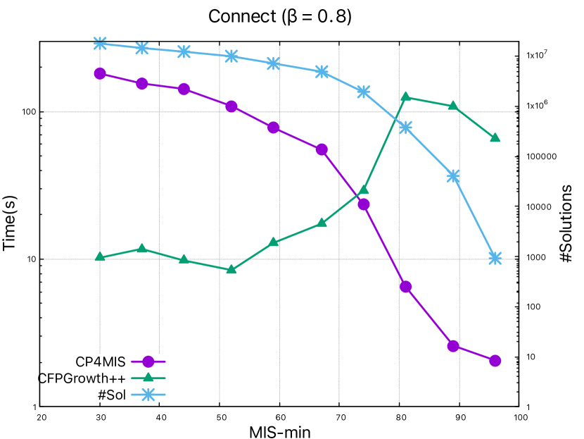
Figure 1: ${\tt CFPGrowth++}$ vs ${\tt CP4MIS}$ varying ${\tt MIS_{min}}$ on $\tt Connect$ with $\beta=0.8$.

5.2.3 RQ3: ${\tt CFPGrowth++}$ vs ${\tt CP4MIS}$ on $Q_{1}$ and $Q_{2}$

Our second experiment compares ${\tt CFPGrowth++(C)}$ to our approach, ${\tt CP4MIS}$, for mining constrained frequent itemsets (queries of type $Q_{1}$ and $Q_{2}$).
${\tt CFPGrowth++(C)}$ (${\tt C}$ is for checker) is a revised version of ${\tt CFPGrowth++}$ with a checker to filter out itemsets violating the constraints.

In Table 4, we report the time, in seconds, for the two approaches and for each instance for mining frequent itemsets of MIS distances bounded above by $ub$ (queries of type $Q_{1}$). We also report the number of solutions for each instance: ${\tt\#sol}$. We selected an $ub$ value for each instance in order to have less than $10K$ solutions.

The main observation that we can draw from Table 4 is that ${\tt CP4MIS}$ outperforms ${\tt CFPGrowth++(C)}$ on all the instances. Comparing to the results of $Q_{0}$, the fact that we strengthen the query with the distance constraint makes the CP resolution more effective. For instance, on $\tt Connect$, ${\tt CP4MIS}$ needed around $14$ minutes to enumerate the $91$ millions of solutions corresponding to $Q_{0}$, where it took only $2$ seconds to return the $1,683$ solutions corresponding to $Q_{1}$ query. Thanks to constraint propagation that drastically reduces the search space. On the other hand, ${\tt CFPGrowth++(C)}$ has no pruning power during the enumeration, and does not take advantage of the additional constraints (the distance constraint in this case) to reduce the search space ($21$ seconds to enumerate the $1,683$ solutions).

To strengthen our findings, we conduct an experiment with $Q_{2}$ query type. In addition to the distance constraint, $Q_{2}$ considers the cardinality constraint i.e., itemsets should have a size of at least $c$. Table 5 reports the time, in seconds, for the two approaches and for each instance acting on $Q_{2}$ query type. We also report the number of solutions of each instance: ${\tt\#sol}$. The parameter $c$ is selected in order to have less than $50$ solutions per instance.

Again, ${\tt CP4MIS}$ is the winner where it is from 4 to $43$ faster than
${\tt CFPGrowth++(C)}$. This is explained by the additional power added to the propagation process during the resolution to enumerate the few solutions present in the huge search space. Where ${\tt CFPGrowth++(C)}$ needs to enumerate the millions of candidates and then filter out the ones violating the user-constraints.

Table 4: ${\tt CFPGrowth++(C)}$ vs ${\tt CP4MIS}$ on the query $Q_{1}$ (time in seconds)

Dataset	$ub$	(a)	(b)	#sol
$\tt Zoo$	2	0.61	0.17	5,765
$\tt Vote$	1	0.82	0.18	2,466
$\tt Anneal$	30	12.95	0.25	1,790
$\tt Chess$	80	5.96	0.27	1,442
$\tt Mushroom$	50	20.20	0.46	2,641
$\tt Connect$	1000	21.28	2.11	1,683
$\tt T40$	100	401.93	107.92	5,846
$\tt Pumsb$	1000	26.97	3.04	1,287
(a):${\tt CFPGrowth++(C)}$; (b):${\tt CP4MIS}$.

Table 5: ${\tt CFPGrowth++(C)}$ vs ${\tt CP4MIS}$ on the query $Q_{2}$ (time in seconds)

Dataset	$ub$	$c$	(a)	(b)	#sol
$\tt Zoo$	2	10	0.62	0.10	14
$\tt Vote$	1	10	1.14	0.13	12
$\tt Anneal$	30	8	12.78	0.18	7
$\tt Chess$	80	8	6.49	0.23	30
$\tt Mushroom$	50	8	19.19	0.36	27
$\tt Connect$	1000	10	20.88	2.03	2
$\tt T40$	100	6	389.80	54.31	14
$\tt Pumsb$	1000	8	27.91	2.86	17
(a):${\tt CFPGrowth++(C)}$, (b):${\tt CP4MIS}$.

5.2.4 RQ4: ${\tt CFPGrowth++}$ vs ${\tt CP4MIS}$ on $Q_{3}$.

For our last experiment, we compares ${\tt CFPGrowth++}$ to ${\tt CP4MIS}$ on a query of type $Q_{3}$ in $k$-patterns mining context. Table 6 reports the different instances selected for our experiment. The instances are selected in order to vary the number of solutions from $0$ to $100K$ $k$-patterns solutions.

Using CP, the problem is expressed using $k$ Boolean vectors (see Section 4.3).

For such problem, a baseline can be the use of specialized algorithm like ${\tt CFPGrowth++}$ combined with a post-processing step. One can imagine two scenarios:

1. The use of ${\tt CFPGrowth++}$ to mine the total number of frequent itemsets with multiple MIS and a generate-and-test search trying to find distinct itemsets satisfying the user-constraints (distance and cardinality constraints in our case). This baseline is coined ${\tt CFPGrowth++(PP)}$ (PP is for post-processing).

2. The use of ${\tt CFPGrowth++(C)}$ to mine the total number of frequent itemsets with multiples MIS satisfying the user-constraints and a generate-and-test search trying to find distinct itemsets. This second baseline is coined ${\tt CFPGrowth++(CPP)}$ (${\tt CPP}$ is for checker + post-processing).

Such baselines can be very expensive. In both cases, the post-processing will generate the possible $k$ combinations of itemsets. Table 6 reports the solutions of $Q_{0}$ and $Q_{2}$ that represent the number of candidates on which the $k$ combinations will be generated for, respectively, ${\tt CFPGrowth++(PP)}$ and ${\tt CFPGrowth++(CPP)}$ baselines.

Table 7 reports the CPU time, in seconds, for each instance and for the three approaches (${\tt CFPGrowth++(PP)}$, ${\tt CFPGrowth++(CPP)}$ and ${\tt CP4MIS}$) acting on $Q_{3}$ query type. We also report the number of solutions of each instance: ${\tt\#sol}$.

The main observation that we can draw from Table 7 is that ${\tt CP4MIS}$ is able to cope with such complex query and to return the $96K$ $k$-patterns solutions in $40$ minutes. This demonstrates again the power of propagation using a CP resolution. On the other hand, the ${\tt CFPGrowth++(PP)}$ baseline timeouts on all instances and ${\tt CFPGrowth++(CPP)}$ on 5 out of the 8 instances. This is an expected result knowing that the baselines have to cope with a massive number of combinations. For instance, on $\tt Connect$ dataset and $k=6$ we have more than $10^{24}$ candidates.

If we take the instance of $\tt Chess$ with $k=6$. Here we have an instance without solution and ${\tt CP4MIS}$ is able to prove it in less than $26$ seconds, where the two baselines reach timeout without proving the unsatisfiability of the instance.

Note that the used checker in ${\tt CFPGrowth++(CPP)}$ allows the baseline to reduce the possibilities, but not enough to avoid the explosion when $k$ grows. ${\tt CFPGrowth++(CPP)}$ first prunes non-solutions using ${\tt CFPGrowth++(C)}$ reducing the search space and thus solving the $\tt Connect$ instance when $k=6$ in $3$ minutes. However, with $k=7$, the search space explodes and ${\tt CFPGrowth++(CPP)}$ is not able to prove no solution exist within the time limit.

To strengthen our observations, we compare the three approaches on $\tt Mushroom$ while varying $k$ in Figure 2. We observe that the two baselines ${\tt CFPGrowth++(PP)}$ and ${\tt CFPGrowth++(CPP)}$ are acting better than ${\tt CP4MIS}$ within a small $k$ (i.e., $k<5$). However, ${\tt CP4MIS}$ scales very well when $k$ grows and it is able to prove that no solution exists on $k=14$ instance in less than $27$ minutes. While the two baselines ${\tt CFPGrowth++(PP)}$ and ${\tt CFPGrowth++(CPP)}$ follow an exponential scale and they reach the one hour time limit when $k$ is equal to, respectively, 5 and 9.

Table 6: Selected instances for k-patterns mining.

Dataset	$\beta$	${\tt MIS_{min}}$	${\tt MIS_{max}}$	${\tt MIS_{avg}}$	${\tt\#sol}_{1}$	$ub$	$c$	${\tt\#sol}_{2}$
$\tt Chess$	0.9	78%	90%	80%	5,553	150	3	932
$\tt Mushroom$	0.9	18%	90%	26%	2,977	3000	2	138
$\tt Connect$	0.9	89%	90%	89%	41,143	300	3	397
$\tt Pumsb$	0.9	88%	90%	88%	7,044	400	3	347
${\tt\#sol}_{1}$ = solutions of $Q_{0}$     ${\tt\#sol}_{2}$ = solutions of $Q_{1}$.

Table 7: ${\tt CFPGrowth++(PP)}$ vs ${\tt CFPGrowth++(CPP)}$ vs ${\tt CP4MIS}$ on the query $Q_{3}$ (time in seconds)

Dataset	$k$	(a)	(b)	(c)	#sol
$\tt Chess$	5	to	61.41	19.10	480
$\tt Chess$	6	to	to	25.42	0
$\tt Mushroom$	9	to	to	862.55	1,407
$\tt Mushroom$	10	to	to	1014.49	0
$\tt Connect$	6	to	182.71	133.68	36,537
$\tt Connect$	7	to	to	143.69	0
$\tt Pumsb$	6	to	199.51	177.80	61,186
$\tt Pumsb$	7	to	to	202.49	0
(a):${\tt CFPGrowth++(PP)}$, (b):${\tt CFPGrowth++(CPP)}$, (c):${\tt CP4MIS}$.

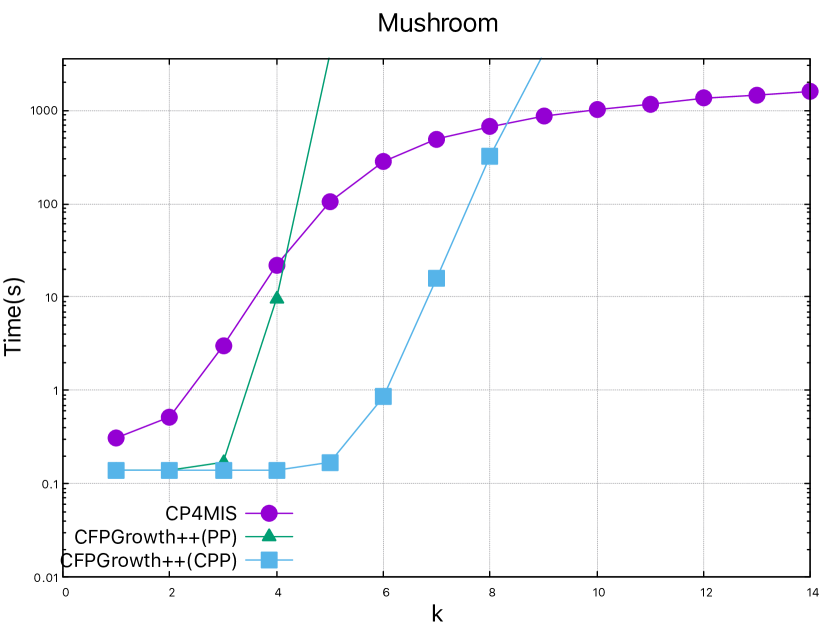
Figure 2: ${\tt CFPGrowth++(PP)}$ vs ${\tt CFPGrowth++(CPP)}$ vs ${\tt CP4MIS}$ for mining k patterns on $\tt Mushroom$.

To sum up, our experimental evaluation shows that a specialized algorithm like ${\tt CFPGrowth}$ is faster on basic queries (e.g., asking for frequent itemsets), but it cannot cope with complex queries in a huge search space and of few solutions. It would need to think and to propose ad-hoc solutions, whereas CP approach enables a novice DM-user to express his query as constraints.

6 Conclusion

In this paper, we have introduced a constraint programming approach for itemset mining with multiple minimum supports MIS. For this, we have defined a new global constraint FreqRare and provided a filtering algorithm that mine frequent itemsets with multiple MIS in backtrack-free manner, given a variable ordering. We have empirically evaluated our CP approach. The experiments showed the performance of our CP model comparing to the specialized approach, ${\tt CFPGrowth++}$. Although ${\tt CFPGrowth++}$ is very efficient on basic queries like mining frequent itemsets, our CP approach outperforms ${\tt CFPGrowth++}$ on complex queries with user-constraints and/or with search space explosion in a $k$-patterns mining. Furthermore, our CP approach provides the user with the flexibility to express any kind of constraints including constraints on MIS without the need to revise the solving process.

References

- [1] M.-B. Belaid, C. Bessiere, and N. Lazaar. Constraint programming for association rules. In Proceedings of the 2019 SIAM International Conference on Data Mining, pages 127–135. SIAM, 2019.
- [2] M.-B. Belaid, C. Bessiere, and N. Lazaar. Constraint programming for mining borders of frequent itemsets. In IJCAI: International Joint Conference on Artificial Intelligence, pages 1064–1070. International Joint Conferences on Artificial Intelligence Organization, 2019.
- [3] W. Gan, J. C.-W. Lin, P. Fournier-Viger, H.-C. Chao, and J. Zhan. Mining of frequent patterns with multiple minimum supports. Engineering Applications of Artificial Intelligence, 60:83–96, 2017.
- [4] T. Guns, S. Nijssen, and L. De Raedt. k-pattern set mining under constraints. IEEE Transactions on Knowledge and Data Engineering, 25(2):402–418, 2011.
- [5] R. U. Kiran and P. K. Re. An improved multiple minimum support based approach to mine rare association rules. In 2009 IEEE Symposium on Computational Intelligence and Data Mining, pages 340–347. IEEE, 2009.
- [6] R. U. Kiran and P. K. Reddy. Novel techniques to reduce search space in multiple minimum supports-based frequent pattern mining algorithms. In Proceedings of the 14th international conference on extending database technology, pages 11–20. ACM, 2011.
- [7] N. Lazaar, Y. Lebbah, S. Loudni, M. Maamar, V. Lemière, C. Bessiere, and P. Boizumault. A global constraint for closed frequent pattern mining. In Principles and Practice of Constraint Programming - 22nd International Conference, CP 2016, Toulouse, France, September 5-9, 2016, Proceedings [7], pages 333–349.
- [8] B. Liu, W. Hsu, and Y. Ma. Mining association rules with multiple minimum supports. In Proceedings of the fifth ACM SIGKDD international conference on Knowledge discovery and data mining, pages 337–341. ACM, 1999.
- [9] L. D. Raedt, T. Guns, and S. Nijssen. Constraint programming for itemset mining. In Proceedings of the 14th ACM SIGKDD International Conference on Knowledge Discovery and Data Mining, Las Vegas, Nevada, USA, August 24-27, 2008 [9], pages 204–212.
- [10] F. Rossi, P. van Beek, and T. Walsh, editors. Handbook of Constraint Programming. Volume 2 of Rossi et al. [10], 2006.
- [11] P. Schaus, J. O. R. Aoga, and T. Guns. Coversize: A global constraint for frequency-based itemset mining. In Principles and Practice of Constraint Programming - 23rd International Conference, CP 2017, Melbourne, VIC, Australia, August 28 - September 1, 2017, Proceedings [11], pages 529–546.
- [12] M.-C. Tseng and W.-Y. Lin. Mining generalized association rules with multiple minimum supports. In International Conference on Data Warehousing and Knowledge Discovery, pages 11–20. Springer, 2001.
- [13] M. Wojciechowski and M. Zakrzewicz. Dataset filtering techniques in constraint-based frequent pattern mining. In Pattern Detection and Discovery, ESF Exploratory Workshop, London, UK, September 16-19, 2002, Proceedings [13], pages 77–91.