ENIGMATIC NEBULOUS COMPANIONS TO THE GREAT SEPTEMBER COMET OF 1882
AS SOHO-LIKE KREUTZ SUNGRAZERS CAUGHT IN TERMINAL OUTBURST

Abstract

I investigate the nature of the transient nebulous companions to the sungrazing comet C/1882 R1, known as the Great September Comet. The features were located several degrees to the southwest of the comet’s head and reported independently by four observers, including J. F. J. Schmidt and E. E. Barnard, over a period of ten days nearly one month after perihelion, when the comet was 0.7 AU to 1 AU from the Sun. I conclude that none of the nebulous companions was ever sighted more than once and that, contrary to his belief, Schmidt observed unrelated objects on the four consecutive mornings. Each nebulous companion is proposed to have been triggered by a fragment at most a few tens of meters across, released from the comet’s nucleus after perihelion and seen only because it happened to be caught in the brief terminal outburst, when its mass was suddenly shattered into a cloud of mostly microscopic debris due possibly to rotational bursting triggered by sublimation torques. The fragment’s motion was affected by a strong outgassing-driven nongravitational acceleration with a significant out-of-plane component. Although fragmentation events were common, only a small fraction of nebulous companions was detected because of their transient nature. The observed brightness of the nebulous companions is proposed to have been due mainly to C₂ emissions, with a contribution from scattering of sunlight by the microscopic dust. By their nature, the fragments responsible for the nebulous companions bear a strong resemblance to the dwarf Kreutz sungrazers detected with the coronagraphs aboard the SOHO space probe. Only their fragmentation histories are different and the latter display no terminal outburst, a consequence of extremely short lifetimes of the sublimating icy and refractory material in the Sun’s corona.

1. Introduction

As celestial spectacle, the Great September Comet of 1882 (C/1882 R1) may not have outclassed its forerunner, the Great March Comet of 1843 (C/1843 D1), another brilliant Kreutz sungrazer. Yet, there is no doubt that the 1882 performer attracted more scientific scrutiny than its rival. Reasons were many, the major ones being as follows.

First, at the most general level, technological innovations on the one hand and scientific progress on the other hand, achieved over the period of four decades between the arrivals of the two comets meant the availability by the 1880s of improved astronomical instrumentation operated by a new generation of dedicated, assiduous, and knowledgeable observers.

Second, cometary science retained its frontline position among the fields of astronomical research in the late 19th century. This is illustrated by the bibliography of E. E. Barnard, one of the era’s most prolific, universal, and influential observers, who also contributed to the subject of this paper. A comprehensive treatise on Barnard’s life and work (Frost 1927) shows that the greatest fraction of his 732 listed publications, 30 percent, did indeed deal with comets, followed by the planets (23 percent) and nebulae (11 percent).

Third, whereas no bright comet very closely approaching the Sun had been reported for some 140 years prior to the 1843 sungrazer, one was under observation over a period of weeks in the early 1880, less than three years before the Great September Comet. The 1880 sungrazer provoked a major controversy about whether it was a return of the 1843 sungrazer (implying the subsequently discredited orbital period of 37 years) or another fragment of a shared parent comet, thus intensifying both theoreticians’ and observers’ interest in this peculiar family of objects.

Fourth, this appeal was still further bolstered by the visual and photographic detection of a cometary object in the Sun’s corona during the solar eclipse on 1882 May 17, just four months before the Great Comet’s perihelion passage. In retrospect, the event was deemed yet another piece of evidence supporting the hypothesis of a genetic relationship among sungrazers forged by the process of recurring fragmentation.

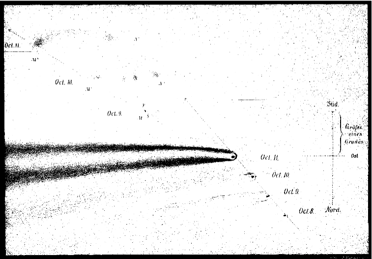
Figure 1.— Schmidt’s (1882a) drawing of the Great September Comet and, what he believed, a single nebulous companion (a.k.a. Schmidt’s comet). Plotted are the positions of the comet’s head in the mornings of 1882 October 9–12, the entire tail on October 12, and a nebulous companion on October 10–12 (Schmidt reckoned the time from Athens local noon, which explains the disparity in the dates). Near the right edge are the picture’s orientation (south up, east to the right) and scale (the brace showing a length of 1^∘).

Fifth, this hypothesis was reinforced to the point of near certainty, when the nuclear condensation of the Great September Comet itself was observed after perihelion to consist of up to six separate points of light lined up like a string of pearls, with the gaps widening with time. While this compelling piece of evidence on a near-perihelion breakup of the original nucleus was being presented literally before the eyes of the observers over a period of months, an independent but rather elusive corroboration was provided by nebulous companions, as explained below. Unlike the multiple nucleus, they were harder to observe and, in addition, transient in nature. Isolated instances of their sighting, in October 1882, were reported by merely a few individuals. They were located at distances of degrees from the head of the Great September Comet and, with one exception, to the southwest of it. This type of feature does not seem to have ever been observed with any other comet and no quantitative explanation of its nature and origin has ever been offered. An investigation of this kind is the objective of the present paper.

2. Reports and Descriptions of Nebulous Companions

In the order of decreasing amount of information provided, the four observers reporting a feature to the southwest of the main comet’s nucleus were Schmidt (1882a), Hartwig (1883), Barnard (1882, 1883a, 1883b), and Markwick (1883). Brooks (1883), a fifth observer, remarked on a feature to the east of the comet. I now present the major points made by each of them in describing their findings.

2.1. Schmidt’s Account

Schmidt (1882a) was the only observer claiming to have seen a nebulous companion to the southwest of the main comet on more than one occasion. He reported its discovery, in the morning of 1882 October 9 UT, as a new comet, noting though that it traveled alongside the Great September Comet (Kreutz 1882). The next morning, October 10.15 UT, Schmidt (1882a) described its appearance in a finder telescope as a fairly bright, crescent-shaped nebulosity, whose vertex was elongated toward the west, the uneven wings extending 1^∘ to the south-southwest and 0${}^{\circ}\!$.5 to the east. The crescent was more condensed near the vertex, fading gradually toward the horns. Measured for position was a point in the elongated vertex, which was more than 3^∘ to the southwest of the main comet’s head.

Some 24 hours later, on October 11.13 UT, the companion consisted of two condensations with wisps and other fainter morphology. Either condensation was about 7^′ to 8^′ in diameter, with no sharp boundary and no nucleus. The condensations were some 87^′ apart, the eastern (seen for the first time) about 20^′ south of the western. The latter, when linked with the elongated vertex on the previous day, implied a daily motion of $\sim$1^∘ radially away from the main comet’s nucleus.

Lastly, on October 12.13 UT both condensations appeared as very dim and large clouds, more than 10^′ across, elongated along a west-east line, with no nucleus whatsoever, yet noticeably condensed, and connected by a faint bridge of fuzzy material. The distance between the condensations was close to 100^′, the eastern again a little, about 10^′, south of the western. The distance of the western feature from the main comet’s nucleus grew by another degree in 24 hours in the same direction as before. Attempts to detect the nebulous companion on the following mornings failed, in part because of deteriorated observing conditions.

Schmidt presented the results of his observations as offsets from the nucleus of the main comet as well as in a drawing that is reproduced in Figure 1. He estimated that his positional measurements of the nebulous companion were uncertain to $\pm$0${}^{\prime}\!$.8 on October 10, to $\pm$3${}^{\prime}\!$.1 on October 11, and to $\pm$2${}^{\prime}\!$.3 on October 12, probably underestimates. Hind (1882), Oppenheim (1882), and Zelbr (1882) independently employed the three positions by Schmidt to compute a parabolic orbit, with mutually incompatible results: for example, Hind determined the argument of perihelion to equal 345^∘ and the perihelion distance 2.8 $R_{\mbox{\scriptsize\boldmath$\odot$}}\!$ , while Oppenheim found for the two elements the values of 108^∘ and 2.0 $R_{\mbox{\scriptsize\boldmath$\odot$}}\!$ ; Zelbr got, respectively, 80^∘ and 0.84 $R_{\mbox{\scriptsize\boldmath$\odot$}}\!$ (sic!). An ephemeris based on Oppenheim’s elements placed the object at $\sim$0.8 AU from the earth on October 10–12, while the main comet was at $\sim$1.4 AU! Zelbr noticed that the results were sensitive to the object’s assumed geocentric distance and that an alternative solution offered a prograde, low inclination orbit with a perihelion distance of about 0.9 AU. He concluded that unless more data became available, the object’s motion would remain indeterminate.

2.2. Hartwig’s Account

Hartwig (1883), as member of a Venus transit expedition, observed a nebulous companion near the comet from aboard a steamship traveling from Hamburg, Germany, to Bahia Blanca, Argentina. At the time of observation, in the morning of October 10, the ship was cruising in the South Atlantic near a longitude of 44^∘W. The nebulous companion appeared as a large nebula, exhibiting a bright nucleus and a symmetric, widely opened fan-shaped tail. Attempts to reobserve the feature in the following mornings, including October 12 under very good conditions, were unsuccessful.

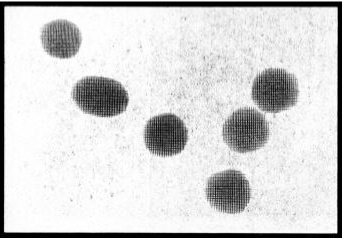
Figure 2.— Barnard’s drawing of six nebulous companions to the Great September Comet that he detected on October 14.43 UT. No scale was presented, but Barnard (1882) indicated that the objects were about 15^′ across. To match approximately his description, south is to the left and east is up. The drawing was provided at a request of the editor of the Sidereal Messenger (Payne 1883).

2.3. Barnard’s Account

Barnard (1882, 1883a) reported that, sweeping to the south of the comet in the morning of October 14, he first picked up a large mass, 15^′ in diameter. It was located between two fainter objects along an east-west line, one in contact, the other a little farther out on the other side. Additional objects were found to the southeast of the trio, including a strongly elongated one. At least six or eight of them were within 6^∘ “south by west” of the main comet’s head. Each looked like a telescopic comet slightly condensed to its center, no rapid motion was apparent. A drawing, reproduced in Figure 2, was submitted by Barnard in response to a request by a journal’s editor (Payne 1883). No positional data of higher accuracy are available. A hazy sky prevented Barnard from searching for the objects the following morning, and he never saw them again; he was very puzzled by their transient nature (Barnard 1883b).

2.4. Markwick’s Account

Markwick (1883) appended his report on the Great Comet from the morning of October 5 by briefly noting that south preceding (i.e., to the southwest of) the comet’s head and about 1${}^{\circ}\!$.5 distant were two wisps of nebulous light. He admitted that he could not say whether they had anything to do with the main comet, and he was unable to recover them in the following mornings.

2.5. Brooks’ Account

While one could speculate that the nebulous companions in the southwest, described in Sections 2.1 to 2.4, may somehow have been related to one another, the cometary mass detected by Brooks’ (1883) 8^∘ to the east of the main comet’s head in the morning of October 21 was unquestionably a feature of different nature. Brooks unfortunately offered only a limited amount of information; he reported that the mass was nearly 2^∘ long and had a slight condensation near its larger end, which pointed toward the Sun. Brooks confirmed his discovery by a second (and last) observation the following morning, when the object was fainter, smaller by at least 0${}^{\circ}\!$.5, and the condensation was barely perceptible. The amount of available information is insufficient to warrant a study of this feature.

2.6. Summary of Companions’ Positional Data

Table 1 presents the positional data on the nebulous companions that I collected from reports by the five observers. For each time of observation, converted to UT, I list the polar coordinates of the nebulous companions’ offsets from the head of the Great Comet. With the exception of Schmidt (1882a) and Hartwig (1883), the position-angle data were reported by the observer, albeit in approximate terms only. Schmidt listed both the separation distance and the offsets in declination and right ascension for the western part of the observed feature. The tabulated position angle was derived by the author from the offsets in right ascension and declination converted to the equinox of J2000. The offsets of the eastern part were handled similarly, after the differences in right ascension and declination from the western part were first added to the latter’s offsets from the head of the main comet. Hartwig’s (1883) published equatorial coordinates for the “middle” of the nebulosity were precessed to J2000 and employed to compute the offsets from the main comet.

3. Nebulous Companions as the Comet’s Fragmentation Products

To start with, I subscribe to the prevailing view that the nebulous companions were genetically related to the Great September Comet, or, put another way, they were its fragments. Of the observers only Markwick (1883) appears to have been noncommittal on this issue. In the following I focus on the nebulous companions situated to the southwest of the main comet. The point one should feel a little uneasy about — and whose explanation should follow from the solution — is that when it comes to the detection of a nebulous companion on a particular day, there are apparent contradictions among the observers. For example, even though both Hartwig and Schmidt reported a nebulous companion at similar positions on October 10 UT, Hartwig, unlike Schmidt, could not recover it under very favorable conditions on the 12th. On the other hand, Schmidt failed to see any trace of a nebulous object on seven consecutive mornings, October 13–19, even though the observing conditions were very favorable on four of them and Barnard detected a swarm of such objects on the 14th. Given the spread of the observers’ sites in the geographic longitude, it almost looks as though the features were only visible over periods as short as a fraction of the day, bringing Barnard’s concern on their transient nature to an extreme. Also peculiar is the circumstance that — contrary to Schmidt’s overtly stated expectations — no reports whatsoever were coming from prestigious southern observatories (such as Cape or Córdoba), more favorably located than Schmidt (Athens, Greece), Barnard (Nashville, Tenn.), or Brooks (Phelps, N.Y.).

In order to get an insight into the process that landed these objects degrees to the southwest of the main comet, I focus on the western condensation of the nebulous companion measured by Schmidt (1882a) on October 10 and 12. If his measurements should indeed refer to the same object, the derived motion should offer constraints on models. Predicating this investigation on the research results for split comets (e.g., Sekanina 1982, Boehnhardt 2004), I accept that the separation distance between a fragment and its parent at a given time is governed by (i) the fragmentation time; (ii) the acquired separation velocity, typically on the order of 1 m s^-1, which is independent or nearly independent of heliocentric distance; and (iii) the differential nongravitational acceleration that the fragment is subjected to after separation. This acceleration is believed to be outgassing-driven (mainly due to the sublimation of water ice), thereby varying approximately as an inverse square of heliocentric distance when less than about 1 AU from the Sun. Its magnitude for fragments of known split comets is usually in a range of 10^-5 to 10^-4 the Sun’s gravitational acceleration (which equals 0.593 cm s^-2 or $29.6\times\!10^{-5}$ AU day^-2 at 1 AU from the Sun), depending on the fragment’s mass, activity, etc. The acceleration correlates with the fragment’s lifespan, being higher for short-lived objects and lower for persistent ones. As a rule, the acceleration is directed essentially away from the Sun and its effects dominate those of the separation velocity. A major exception is presented by the population of SOHO dwarf Kreutz sungrazers, whose examination by Sekanina & Kracht (2015) demonstrated that (i) the normal component of the nongravitational acceleration was comparable in magnitude to the radial component and (ii) the acceleration’s overall magnitude was in the range of 0.02 to nearly 1 Sun’s gravitational acceleration (sic!) between 8 and 15 $R_{\mbox{\scriptsize\boldmath$\odot$}}\!$ from the Sun.

An important dynamical property of fragments of split comets whose motions are dominated by the radial nongravitational acceleration is that, relative to the primary (most massive) fragment, the motions of secondary (less massive) fragments are directionally constrained: their positions in the orbital plane are restricted to a sector of less than 180^∘, subtended by the prolonged radius vector, $RV$ (the anti-solar direction) and the vector of the negative orbital-velocity vector, $-V$ (the direction behind the comet). To verify compliance with this constraint is trivial.

To subject the Schmidt nebulous companion to this test, I list the position angles, measured from the nucleus of the Great September Comet, in Table 2: for the radius vector in column 4, for the negative velocity vector in column 5. Because the orbit’s curvature at the relevant heliocentric distances is very small, the two vectors make an angle of nearly 180^∘, yet it is the northern sector that is slightly less than 180^∘ wide. For example, for October 10.15 UT a nebulous companion would satisfy the condition if its position angle were smaller than 84${}^{\circ}\!$.8 or greater than 267^∘. Since the Schmidt nebulous companion was near position angle of 240^∘, it did not satisfy the condition and its motion was obviously not dominated by the radial nongravitational acceleration, regardless of the fragmentation time.

The obvious alternative is to consider the nebulous companion’s motion determined mainly by a separation velocity. Schmidt’s observations of the nebulous companion’s western condensation suggest a motion rate of about 1^∘ per day at a geocentric distance of 1.4 AU, assuming the nebulous companion was in the general proximity of the main comet. This transforms to an average projected velocity relative to the main comet of approximately 40 km s^-1. Even before accounting for a foreshortening effect, this is more than four orders of magnitude higher than an expected relative velocity, ruling out the separation velocity as the trigger.

4. Nongravitational Acceleration Normal to the Orbit Plane

Another option is to contemplate that the nebulous companion’s motion relative to the main comet was governed by a nongravitational acceleration with a strong contribution from the component normal to the orbital plane, a scenario emulating the behavior of the SOHO Kreutz sungrazers. To examine this case, I first consider a fragment that is moving with the comet except for its increasing distance from the orbital plane. I consider a right-handed orthogonal rotating heliocentric coordinate system in which the $z$-axis points to the comet’s orbital pole, the $x$-axis to the comet’s nucleus, and the $y$-axis completes the system. The position of the main comet’s nucleus at time $t$ is determined by the coordinates $\{r(t),0,0\}$, while the nebulous companion, subjected to a nongravitational acceleration normal to the orbital plane, is assumed to be located at a point {$r(t),0,z(t)$}. The task is to determine the distance $z(t)$ from the orbital plane as a function of time. To make the problem easily tractable, I use some (reasonable) approximations.

Let a nebulous companion be released from the comet’s nucleus after perihelion, at time $t_{\rm frg}$, when its heliocentric distance is $r_{\rm frg}=r(t_{\rm frg})$. Let the orbit of the main comet be approximated by a parabola, so that the relation between time $t$ (in days) and heliocentric distance $r(t)$ (in AU) is expressed by

$$t=t_{\pi}+{\displaystyle\frac{\sqrt{2}}{3k}}(r\!+\!2q)\sqrt{r\!-\!q},$$ (1)

where $t_{\pi}$ is the time (in days) of the main comet’s perihelion passage and $k$ is the Gaussian gravitational constant, $k=0.0172021$ AU${}^{\frac{3}{2}}$ day^-1. Let the nebulous companion be subjected to a nongravitational acceleration normal to the orbital plane, whose variation with heliocentric distance follows an inverse square power law. As a result, the nebulous companion begins to recede from the comet in a direction perpendicular to the orbital plane with a systematically increasing velocity $\dot{z}(t)$,

$$\dot{z}(t)=\int_{t_{\rm frg}}^{t}\!\!\!\frac{k^{2}\Gamma_{\!\rm N}}{r^{2}}\,dt,$$ (2)

where $k^{2}/r^{2}$ is the Sun’s gravitational acceleration at $r$ and $\Gamma_{\rm N}$ is a dimensionless constant that determines the normal component of the nongravitational acceleration as a fraction of the Sun’s gravitational acceleration. It is noted that $\dot{z}(t_{\rm frg})=0$ and that the denominator in Equation (2) should strictly read $r^{2}\!+\!z^{2}$; the approximation is acceptable as long as $z\ll r$. The distance from the comet (and the orbital plane) at time $t$ is

$$z(t)=\!\int_{t_{\rm frg}}^{t}\!\!\!\!\dot{z}(t)\,dt.$$ (3)

One can now proceed in one of two possible ways. One is to use Kepler’s second law and substitute true anomaly for time as the integration variable. Followed below is the other option, in which $dt$ is expressed in terms of $dr$ by differentiating Equation (1),

$$dt=\frac{r}{k\sqrt{2}\sqrt{r-q}}\,dr.$$ (4)

The integration of the velocity expression (2) gives for $z(t)$ from Equation (3) with help of the relation (4):

$$z(t) = \frac{\Gamma_{\!\rm N}}{\sqrt{q}}\!\int_{r_{\rm frg}}^{r}\!\!\frac{r}{\sqrt{r-q}}\!\left[\arcsin\!\sqrt{q/r_{\rm frg}}-\!\arcsin\!\sqrt{q/r}\right]\!dr$$ (5)

$$= 2q\Gamma_{\!\rm N}\!\!\int_{\sqrt{q/r}}^{\sqrt{q/r_{\rm frg}}}\frac{\arcsin\sqrt{q/r_{\rm frg}}-\arcsin u}{u^{4}\sqrt{1\!-\!u^{2}}}\,du.$$

Since the integration of the expression in closed form is rather convoluted, I prefer to expand the functions into polynomials,

$$\arcsin u = u+{\textstyle\frac{1}{6}}u^{3}+\ldots,$$

$$(1\!-\!u^{2})^{-\frac{1}{2}} = 1+{\textstyle\frac{1}{2}}u^{2}+{\textstyle\frac{3}{8}}u^{4}+\ldots,$$ (6)

and, assuming that $q\ll r_{\rm frg}<r$, neglect all terms higher than $u^{2}$. Substituting $\Re=\sqrt{r/r_{\rm frg}}>1$, I obtain a solution

$$z(t)={\textstyle\frac{1}{3}}\Gamma_{\!\rm N}\left[r_{\rm frg}F(\Re)+3qG(\Re)\right],$$ (7)

where

$$F(\Re) = (\Re-1)^{2}(2\Re+1),$$

$$G(\Re) = (\Re-1)-\ln\Re.$$ (8)

The ratio $G(\Re)/F(\Re)$ decreases from $\frac{1}{6}$ when $\Re\!\rightarrow\!1$ to zero when $\Re\!\rightarrow\!\infty$, so that the second term in Equation (7) always contributes only a fraction of the first. To test the range of $\Gamma_{\!\rm N}$ required to fit the data in Table 1, I first consider a case of an angular distance of 4^∘ at a heliocentric distance of 0.9 AU and a geocentric distance of 1.4 AU; the required nongravitational accelerations $\Gamma_{\!\rm N}$ are found to be high, from 10 percent of the solar gravitational acceleration for a fragment separating at a heliocentric distance 0.1 AU (1 day after perihelion, September 18.7 UT) to 7.3 times the solar gravitational acceleration for a fragment separating at 0.7 AU from the Sun (16.3 days after perihelion, October 4.0 UT)!

This exercise offers only a crude estimate, because the projection conditions have not as yet been considered. In addition, a nebulous companion’s motion in a strictly perpendicular direction to the orbital plane is unrealistic, as documented by a simple calculation of the direction of the projected normal to the orbital plane. For the times of Schmidt’s observations of the nebulous companion, the position angle of the northern orbital pole was essentially constant, equaling 166^∘. The nebulous companion surely did not travel along the normal to the orbital plane, given the difference of about 70^∘ between the observed and expected position angles.

Figure 3.— Nebulous companion to comet C/1882 R1 subjected to an outgassing-driven nongravitational acceleration, whose radial component, measured in units of the Sun’s gravitational acceleration, is $\Gamma_{\!\rm R}$ and the normal component is $\Gamma_{\!\rm N}$. Left: View from a point in the orbital plane. The Sun is to the left, FRG is the point of separation, from the main comet, of the fragment whose debris the nebulous companion represents. CN and CP are the positions of, respectively, the main comet’s head and the nebulous companion at the time of observation, $t$. PT is the companion’s footprint in the orbital plane. The heliocentric distance of the point of separation is $r_{\rm frg}$, while $r(t)$ is the comet’s heliocentric distance at $t$. The distance of the nebulous companion from the main comet at time $t$ is $s(t)$, from the orbital plane $z_{\ast}(t)$. The distance of the companion’s footprint from the main comet at time $t$ is $r_{\ast}(t)$. Right: In projection onto the plane of the sky. CN, CP, and PT refer to the same points as on the left. The angular distance of the companion from the main comet is $\widehat{s}$, from its footprint in the orbital plane is $\widehat{z}_{\ast}$, and the angular distance of the footprint point from the main comet is $\widehat{r}_{\ast}$. The position angle of the companion from the main comet is $P$, the position angle of the radius vector measured at the main comet is $P_{\rm RV}$, and the position angle of the normal to the orbital plane measured at the companion is $P_{\rm N}$. The measured quantities are $P$ and $\widehat{s}$, while $P_{\rm RV}$ and $P_{\rm N}$ can be derived from the orbital elements and the companion’s position.

5. Two-Dimensional Model for a Nebulous Companion’s Motion

Even though the nongravitational acceleration in a direction normal to the orbital plane was positionally the most consequential effect, the in-depth treatment of the motions of the eight SOHO sungrazers by Sekanina & Kracht (2015) showed that the normal component was generally on a par with the acceleration’s radial component. Consistent with this finding, I revise the scenario from the foregoing section, requiring now that the nebulous companion’s “footprint” in the orbital plane be not the comet’s nucleus but a hypothetical particle that separated from the nucleus at time $t_{\rm frg}$ under a radial nongravitational acceleration of $\Gamma_{\!\rm R}$. Because of the nature of sungrazing orbits, this particle was moving essentially along the radius vector (except very near the Sun, a case not contemplated here), receding from the nucleus to a distance of $r_{\ast}(t)$ over a period of time $t\!-\!t_{\rm frg}$. Accordingly, in the system introduced in Section 4, the coordinates of the nebulous companion’s footprint in the orbital plane at time $t$ are $\{r\!+\!r_{\ast}(t),0,0\}$ and the coordinates of the nebulous companion itself are $\{r\!+\!r_{\ast}(t),0,z_{\ast}(t)\}$, where, in analogy to Equation (7),

$$r_{\ast}(t)={\textstyle\frac{1}{3}}\Gamma_{\!\rm R}[r_{\rm frg}F(\Re)+3qG(\Re)]$$ (9)

and the $z_{\ast}$ coordinate of the nebulous companion is then

$$z_{\ast}(t)={\textstyle\frac{1}{3}}\Gamma_{\!\rm N}[r_{\rm frg}F(\Re_{\ast})+3qG(\Re_{\ast})],$$ (10)

where $\Re_{\ast}=\sqrt{(r\!+\!r_{\ast})/r_{\rm frg}}$.

The task now is to find out under what circumstances could this simple model fit the motion of the nebulous companion observed by Schmidt between October 10 and 12 UT. I ignore the middle observation, on October 11 UT, which was described by Schmidt as the most uncertain of the three anyway. The line of attack is described schematically in Figure 3. The left panel shows a view of the post-perihelion branch of the orbit from a point in the orbital plane. From the left to the right are the Sun; the point of separation of the nebulous companion from the comet’s nucleus (FRG); the comet’s position (CN) at time $t$; and the nebulous companion’s position (CP) and footprint in the orbital plane (PT) at time $t$. The distances $r_{\rm frg}$, $r(t)$, $r_{\ast}(t)$, $z_{\ast}(t)$, and the separation distance of CP from CN, $s(t)$, are marked. The right panel transfers the picture from space onto the plane of the sky. The three vertices of the spherical triangle, CN, PT, and CP, are pairwise connected by great circular arcs: $\widehat{s}$ links CN with CP, $\widehat{r}_{\ast}$ links CN with PT, and $\widehat{z}_{\ast}$ links CP with PT. One knows two of the three angles: (i) the angle at the vertex CN equals the difference between the position angle of the prolonged radius vector, $P_{\rm RV}$, and the position angle of the nebulous companion measured from the comet’s nucleus, $P$; and (ii) the angle at the vertex CP equals the difference between $P$ and the position angle of the normal to the orbital plane, $P_{\rm N}$. The arcs $\widehat{r}_{\ast}$ and $\widehat{z}_{\ast}$ are then determined from

$$\sin\widehat{r}_{\ast} = \kappa\sin(P\!-\!P_{\rm N})$$

$$\sin\widehat{z}_{\ast} = \kappa\sin(P_{\rm RV}\!-\!P),$$ (11)

where

$$\kappa=\sin\widehat{s}\left\{\!\raisebox{0.0pt}[4.30554pt][4.30554pt]{1}-\left[\cos(P_{\rm RV}\!-\!P)\cos(P\!-\!P_{\rm N})\right.\right.$$

$$\left.\left.-\cos\widehat{s}\,\sin(P_{\rm RV}\!-\!P)\sin(P\!-\!P_{\rm N\!})\right]^{2}\right\}^{\!-\frac{1}{2}}\!\!.$$ (12)

Next, the angular distances $\widehat{r}_{\ast}$ and $\widehat{z}_{\ast}$, which I express in degrees, need to be converted to the linear distances $r_{\ast}$ and $z_{\ast}$ that will be reckoned in million km. This requires to account for the effects of geocentric distance and projection foreshortening. Given that 1^∘ projected onto the plane of the sky equals 2.611 million km at 1 AU from the earth, the conversion is accomplished by the relations:

$$r_{\ast}(t) = 2.611\,\Delta(t)\,f_{\rm RV}\!(t)\>\widehat{r}_{\ast},$$

$$z_{\ast}(t) = 2.611\,\Delta(t)\,f_{\rm N}(t)\>\widehat{z}_{\ast},$$ (13)

where $\Delta(t)$ is the comet’s geocentric distance at time $t$ listed in Table 2 (the distance between the nucleus and the nebulous companion being neglected) and $f_{\rm RV}(t)$ and $f_{\rm N}(t)$ are the projection foreshortening corrections along the radius vector and the normal to the orbital plane, respectively. Numerically the factor $f_{\rm RV}$ is related to the angle $\psi_{\rm RV}(t)$ between the line of sight and the plane normal to the radius vector by

$$f_{\rm RV}(t)=\sec\psi_{\rm RV}(t)\geq 1.$$ (14)

This angle is equal to $\psi_{\rm RV}=|90^{\circ}\!-\!($C-S-E)$|$, where (C-S-E) is the angle Comet-Sun-Earth listed in Table 2. At Schmidt’s October 10–12 observations $\psi_{\rm RV}$ varied between 3${}^{\circ}\!$.9 and 5${}^{\circ}\!$.8, so that $f_{\rm RV}$ did not exceed 1.005. The similarly defined angle $\psi_{\rm N}$ varied from 10${}^{\circ}\!$.5 on October 10 to 11${}^{\circ}\!$.2 on October 12, implying $f_{\rm N}$ in a range from 1.017 to 1.019.

The objective is to find a solution providing the time of the nebulous companion’s separation from the comet’s nucleus that would simultaneously fit Schmidt’s observations from October 10.15 UT, referred to below as time $t_{1}$, and October 12.13 UT, or time $t_{2}$. More specifically, the values of $r_{\ast}(t_{1})$, $z_{\ast}(t_{1})$, $r_{\ast}(t_{2})$, and $z_{\ast}(t_{2})$ derived from the observed data via Equations (13) should equal the values computed from Equations (9) and (10), respectively. Since the latter depend on the nongravitational acceleration’s components $\Gamma_{\!\rm R}$ and $\Gamma_{\!\rm N}$, which are, next to $r_{\rm frg}$, additional free parameters, it is only necessary that the ratios $r_{\ast}(t_{2})/r_{\ast}(t_{1})$ and, simultaneously, $z_{\ast}(t_{2})/z_{\ast}(t_{1})$ from the proposed scenario match those derived directly from the observations.

Solving this problem is convolved not only because the search has to be conducted by trial and error, but primarily because the observations are burdened by large errors. The uncertainty is of two kinds: one is triggered by a great difficulty to bisect the brightest point of a fuzzy feature of large dimensions, a problem that Schmidt kept complaining about; the other, even more severe, is prompted by the nebulous companion’s ever changing morphology, which makes the position of the brightest spot refer to different parts of the feature over time; the observer’s measurements of the nebulous companion are then rather misleading. The bottom line is that the search for a solution should aim at examining a fit to not only the reported position, but to a class of positions in its general proximity to determine an optimum case.

Armed with this strategy, I found that the rate of increasing separation of the nebulous companion from the main comet is fitted best by assuming that the nebulous companion broke off at a heliocentric distance of 0.665 AU, one week before Schmidt’s October 10 observation. The nebulous companion’s observed motion in the orbit’s plane was matched very well, but moderate corrections were required in the direction normal to the plane, 12^′ to the north on the 10th and 26^′ to the south on the 12th, equivalent to changes of a few degrees in the position angle. The results in Table 3 show that fitting the motion of the nebulous companion relative to the comet entailed an extremely high nongravitational acceleration in the radial direction, more than five times higher than the Sun’s gravitational acceleration. In the normal direction the effect was smaller, but still exceeding the Sun’s acceleration.

The source of these huge forces is unknown and suspicious, and their existence dubious. It is easy to show that they cannot come from the sublimation of ices by the nebulous companion’s material. An order-of-magnitude estimate is obtained from the well-known conservation-of-momentum condition: If ${\cal M}$ is the nebulous companion’s mass at time $t$, $\dot{\cal M}_{\rm subl}$ an average mass-loss rate by outgassing during the nebulous companion’s lifetime, between $t$ and $t\!+\!\tau_{\rm life}$, $V_{\rm subl}$ a collimated sublimation velocity (not exceeding 0.36 km s^-1), and $\gamma_{\rm subl}$ an average outgassing-driven nongravitational acceleration, the momentum condition, ${\cal M}\gamma_{\rm subl}=V_{\rm subl}\dot{\cal M}_{\rm subl}$, implies for the nebulous companion’s sublimation lifetime

$$\tau_{\rm life}=\frac{\cal M}{\dot{\cal M}_{\rm subl}}=\frac{V_{\rm subl}}{\gamma_{\rm subl}}.$$ (15)

With the acceleration data from Table 3 near 0.9 AU, I find $\gamma_{\rm subl}=4.15$ cm s^-2, and the expected sublimation lifetime is

$$\tau_{\rm life}<0.1\;{\rm day},$$ (16)

which is two orders of magnitude shorter than the companion’s time of flight from Table 3. The obvious difficulty with this scenario is to explain the nebulous companion’s enormous relative velocity implied by its motion of about 1^∘ per day that Schmidt (1882a) specifically noted. This angular rate is equivalent to a projected linear velocity of about 42 km s^-1 if the nebulous companion is crudely at the same geocentric distance as the main comet. This enormous relative velocity ought to be reached over a very short period of time, as the nebulous companion would have otherwise been brighter earlier and should have been detected sooner by many observers on numerous occasions.

From the standpoint of the proposed hypothesis, the distances $r_{\ast}$ and $z_{\ast}$ are tightly constrained by their ratio from the two dates. For example, the ratio $r_{\ast}$(Oct 12)/$r_{\ast}$(Oct 10) ought to be 1.55; it equals only 1.12 and 1.28 when the separation time $r_{\rm frg}$ is 0.1 AU and 0.5 AU, respectively. It equals 1.55 only when $r_{\rm frg}=0.665$ AU. Similarly the ratio of 1.76 for $z_{\ast}$. There is no escape from the constraint of recent separation and thus of unrealistically high nongravitational accelerations.

6. Introducing the Separation Velocity

In an effort to mitigate these disparities, I now assume that the nebulous companion departed the comet with a separation velocity, whose radial and normal components were $V_{\rm R}$ and $V_{\rm N}$, respectively, before it became subject to the nongravitational acceleration. This premise requires that the expressions for $r_{\ast}$ and $z_{\ast}$ be corrected to include the respective velocity contributions as functions of heliocentric distance.

The expressions for the radial and normal components are again of the same type; I call $r_{0}$ the integrated effect of the radial component of the separate velocity, $V_{\rm R}$; and $z_{0}$, the integrated effect of the normal component, $V_{\rm N}$,

$$r_{0}(t) = \int_{t_{\rm frg}}^{t}\!\!\!\!V_{\rm R}\,dt=\frac{V_{\rm R}}{k\sqrt{2}}\int_{r_{\rm frg}}^{r}\!\frac{r}{\sqrt{r\!-\!q}}\,dr,$$

$$z_{0}(t) = \int_{t_{\rm frg}}^{t}\!\!\!\!V_{\rm N}\,dt=\frac{V_{\rm N}}{k\sqrt{2}}\int_{r_{\rm frg}}^{r}\!\frac{r}{\sqrt{r\!-\!q}}\,dr,$$ (17)

where once again I use the parabolic approximation. Integrating the expression for $r_{0}(t)$ I find

$$r_{0}(t) = \frac{V_{\rm R}\sqrt{2}}{3k}\!\left[\raisebox{0.0pt}[12.91663pt][12.91663pt]{}r^{\frac{3}{2}}\!\left(1\!-\!{\displaystyle\frac{q}{r}}\right)^{\!\frac{1}{2}}\!\!\left(1\!+\!{\displaystyle\frac{2q}{r}}\right)\right.$$ (18)

$$\left.-r_{\rm frg}^{\frac{3}{2}}\!\left(\!1\!-\!{\displaystyle\frac{q}{r_{\rm frg}}}\!\right)^{\!\frac{1}{2}}\!\!\left(\!1\!+\!{\displaystyle\frac{2q}{r_{\rm frg}}}\!\right)\!\right].$$

Writing the square root expressions as series and neglecting the $(q/r_{\rm frg})$ terms of powers 2 and higher, one has:

$$r_{0}(t)=\frac{V_{\rm R}\sqrt{2r_{\rm frg}}}{3k}\!\left[r_{\rm frg}(\Re^{3}\!-\!1)+{\textstyle\frac{3}{2}}q(\Re\!-\!1)\right],$$ (19)

where $\Re=\sqrt{r(t)/r_{\rm frg}}$. The heliocentric distance of the nebulous companion’s footprint in the orbital plane at time $t$ is now equal to $r(t)\!+\!r_{\ast}(t)\!+\!r_{0}(t)$. Replacing in (19) $V_{\rm R}$ with $V_{\rm N}$ and the ratio $\Re(t)$ with $\Re_{\ast}(t)=\sqrt{[r(t)+r_{\ast}(t)+r_{0}(t)]/r_{\rm frg}}$, one obtains the expression for the normal coordinate of the nebulous companion at time $t$, $z_{0}(t)$.

Adding the separation velocity to the list of free parameters makes their number one too many, allowing no unique solution. I show the dependence on the choice of the heliocentric distance at separation in Table 4. Comparison with Table 3 suggests that the introduction of the separation velocity affects the magnitude of the nongravitational acceleration only slightly, but shows that the magnitude of the separation velocity is very sensitive to the choice of the heliocentric distance at separation, increasing rapidly in both directions. The acceleration — both in the radial and normal directions — diminishes with increasing heliocentric distance at separation when it exceeds 0.7 AU, but its moderate decrease is compensated by a sharp increase in the radial separation velocity. Over all, the introduction of the separation velocity fails to make the solutions more realistic than before. This exercise also confirms that a separation velocity on the order of 10 m s^-1 or lower has practically no effect on the solution.

The last option in this category of solutions, based on the assumption that the nebulous companion’s motion relative to the main comet was triggered by the separation velocity alone, with no contribution from the nongravitational acceleration, does not help anything, as expected. The radial motion is fitted best for a heliocentric distance at separation of 0.77 AU (only about a week before Schmidt’s October 10 observation), but the required radial separation velocity is fully 39 km s^-1!

7. Resolving the Problem

All attempts aimed at fitting Schmidt’s (1882a) positional observations over three consecutive days in terms of the motion of a single nebulous companion have failed to offer a dynamically meaningful solution. The feature described by Schmidt as the western condensation of the nebulous companion on October 10, 11, and 12 UT must inevitably have been three different objects. Similarly, the eastern condensation of the companion on October 11 could not possibly have been the same mass as on October 12. In addition to the inexplicably rapid motion relative to the main comet, this conclusion is supported by at least two other pieces of evidence. One, Schmidt’s descriptions of the morphology varied from day to day, showing little or no morphological similarity (Section 2.1). And two, Barnard (1883b) suggested that these features were omnipresent in the region southwest of the main comet in mid-October, but complained about “their visibility being so transient” (Section 2.3).

I propose that the clue to solving the problem of nebulous companions is the key role of terminal outburst. In general, outbursts, which last from a fraction of a day to many days or weeks, are common manifestations of cometary activity. Some comets undergo giant explosions that appear to have no effect on their well-being. A quintessential example is a pair of huge outbursts, 40 days apart, experienced by comet 41P/Tuttle-Giacobini-Kresák in its 1973 return; in either episode, the brightness soared by 8–9 magnitudes to the peak in a matter of hours and then subsided at a similarly steep rate. Since 1973 the comet has completed eight revolutions about the Sun apparently in perfect health.

By contrast, the expression terminal outburst derives from the observation that this event often is experienced by cometary nuclei or their fragments shortly before their sudden disintegration. A possible mechanism for such a cataclysmic event could be rotational instability triggered by torques from strongly anisotropic outgassing, resulting eventually in rotational disruption, as discussed by Jewitt (2021). In line with the morphological diversity of the nebulous companions of the Great September Comet, I hereby propose that they were triggered by poorly-cemented minor fragments of the comet’s nucleus and seen only because they happened to be caught in the brief terminal outburst, when their mass was suddenly shattered into clouds of mostly microscopic debris. Only a small fraction of nebulous companions was in fact detected not only because of their transient nature, but also because only some minor fragments were poorly cemented to the degree that they disintegrated this early after their birth; other fragments could survive a greater part of the orbit or nearly the entire orbit.

The birth of minor fragments giving rise to the nebulous companions is linked to the process of breakup of the comet’s nucleus, which apparently occurred merely hours after perihelion (Sekanina & Chodas 2007). Such minor fragments may have separated in the aftermath of, rather than during, the prime event, an issue of no major import. However, in order to end up degrees to the southwest of the comet’s head, these fragments must have been subjected to major nongravitational accelerations in both the radial and normal directions. The out-of-plane effect may have been the product of high-obliquity rotation. In any case, the similarity to the behavior of the SOHO dwarf Kreutz sungrazers is striking. The only distinctions are their different fragmentation histories and the SOHO sungrazers’ absence of the terminal outburst, unquestionably a consequence of extremely short lifetimes of both icy and dust grains vigorously sublimating in the high-temperature environment of the solar corona.

The proposed outburst scenario implies a very short lifetime for the observed nebulous companions, certainly less than 24 hours, which is why Schmidt’s (1882a) observations make sense only if they refer to unrelated objects. Indeed, if a gradually sublimating fragment is just of about the right size, its debris is detected only at and near the peak of the terminal outburst in the small telescopes used in 1882. The debris of fragments that are smaller than this critical size fails to reach the threshold of detection even at the peak of the terminal outburst, thus remaining unobserved. On the other hand, for fragments of larger dimensions, which are fewer to begin with, the process may take longer and be completed at larger heliocentric distances, thus escaping detection. Also, larger fragments are subjected to lower accelerations and they may not venture as far away from the orbital plane as do smaller fragments. In general, as part of the process of nuclear fragmentation of the Great September Comet, the nebulous companions appear to have represented a detached, transient extension to the diffuse sheath of material that was observed to encompass the major nuclear fragments over a protracted period of time.

It is disappointing that none of the observers reported a magnitude estimate for any of the nebulous companions. Schmidt (1882a) noted that the feature he observed appeared as a nebula “easily perceptible in the finder” of the telescope, but he offered no information on what the expression meant in magnitude terms. He even failed to specify the finder’s aperture size. Hartwig (1883) observed the main comet with a 5-cm f/15 telescope and I presume that he used this instrument for sighting the nebulous companion as well. Markwick (1883) employed a 7-cm achromatic for his Pietermaritzburg observations, while Barnard’s telescope was a 13-cm f/15 Byrne refractor. I adopt a crude guess for an apparent (as well as absolute) magnitude 9 for the nebulous companions, inferred from indirect information based on Schmidt’s remarks on other objects he observed with this finder. The guess is in line with what he said about his first observation, on 1880 December 30, of comet C/1880 Y1 (Pechüle). Schmidt (1881b) wrote that the comet was clearly seen in the finder of the 11-cm refractor, estimating its condensation at magnitude 9. Similarly, he remarked that comet C/1881 K1 (Tebbutt) was an easy object in the same finder on 1881 October 13 (Schmidt 1882b); the following day Pickering et al. (1900) measured the comet’s brightness with a visual photometer and found magnitude 9.2. Schmidt (1881c) also felt comfortable with using this same finder for examining stars of magnitude 9. It appears that objects of magnitude 9 were the finder’s typical-brightness standard. His observations of C/1882 R1 also provided a constraint on the finder’s limiting magnitude (Schmidt 1883); referring obviously to the comet’s condensation, he noted that it was still visible in the finder at the end of March 1883. The light curve by Sekanina (2002) suggests that its apparent magnitude at the time was 10.0, so that the limiting magnitude of the finder may have been close to magnitude 11.

The estimated absolute magnitude of the nebulous companions allows one to provide constraints on the mass consumed in the terminal outburst. The peak visual brightness of a disintegrating porous icy dust conglomerate depends on both the released amount of molecular species that radiate in the visible spectrum, C₂ in particular, and on the total cross-sectional area of the disintegrated solid material that scatters sunlight. Because of a fairly small heliocentric distance, atomic sodium could also contribute to the visual brightness but probably only marginally. Below I consider two extreme cases, the entire effect being due to (i) the abundance of C₂ molecules and (ii) scattering by microscopic dust.

The first case employs A’Hearn & Millis’ (1980) relationships (i) between the absolute visual magnitude and the production rate of C₂ (normalized to 1 AU from the Sun) that is required to sustain it; and (ii) between the normalized production rates of C₂ and H₂O, the latter approximated by the rate of OH. Combined with the standard water-ice sublimation model for rapidly rotating comets, one can use the relationships to calculate the time needed to completely sublimate a disintegrated fragment of a given size in an outburst with the peak absolute magnitude of 9 and the corresponding amplitude of the outburst measured from a base level of brightness given by outgassing from a spherical nucleus of the same dimensions. For an assumed bulk density of 0.5 g cm^-3 I find that to reach the absolute magnitude 9, a disintegrated spherical fragment 10 meters across needs near 1 AU from the Sun 1.0 hr to sublimate away; 13 meters across needs 2.2 hr; 16 meters, 4.0 hr; and 20 meters, 7.9 hr. The outburst amplitudes (relative to sunlight scattered by the surface of the inactive object of the given dimensions) are, respectively, 12.5 mag, 11.8 mag, 11.2 mag, and 10.6 mag, so that the relevant absolute magnitudes vary, accordingly, from 21.5 mag to 19.6 mag. Because the photodissociation lifetime of C₂ at the pertinent heliocentric distances amounts to about 1 day or a little less and because the observed lifetime of the nebulous companions is about the same (as they are not seen for two days in a row), an outburst cannot last longer than a small fraction of a day. Correspondingly, the fragment’s diameter at the outburst’s onset should not exceed $\sim$15 meters.

In the other case a fragment that just lost all its volatiles is assumed to disintegrate into an optically thin cloud of microscopic dust particles. The total projected cross-sectional area, which at a given particle albedo determines the required brightness, is the sum of the individual particles’ cross-sections. At an assumed geometric albedo of 4 percent, the absolute magnitude 9 implies a cross-sectional area of 8800 km². If made up of dust grains 0.2 micron across and density 3 g cm^-3, the companion comes out to be $1.8\times\!10^{9}$ g in mass and, at a bulk density of 0.5 g cm^-3, 24 meters initially across. With the terminal dimensions now larger, this scenario is clearly inferior to the C₂ based case. Also, dust outbursts have a tendency to a slowly declining post-peak brightness, inconsistent with the observational constraint.

The next issue is the rate at which the fragment was sublimating away between separation and the terminal outburst. A solution to this problem provides an estimate of how much larger was the fragment at its birth than at the end of its lifespan. The mass sublimation rate, $\dot{Z}(t)$ (in g cm^-2 day^-1), makes the fragment’s surface recede at a rate of $\dot{Z}(t)/\rho$ (in cm day^-1), where $\rho$ is the bulk density. The rate at which the fragment’s diameter, $D(t)$, is diminishing with time at $t$, is

$$dD(t)=-\frac{2\dot{Z}(t)}{\rho}dt.$$ (20)

I now consider the sublimation of water ice from a rapidly rotating spherical object, in which case one can write approximately at the relevant heliocentric distances

$$\dot{Z}(t)=\dot{Z}_{0}\left[\frac{r_{\oplus}}{r(t)}\right]^{2},$$ (21)

where $r_{\oplus}=1$ AU and $\dot{Z}_{0}\simeq 0.8$ g cm^-2 day^-1. Integrating from the time of separation, when the comet’s distance from the Sun was $r_{\rm frg}$ and the fragment’s diameter $D_{\rm frg}$, to the time of terminal outburst, when the distance was $r_{\rm fin}$ and the diameter $D_{\rm fin}$, one finds, using Equation (4),

$$D_{\rm fin} = D_{\rm frg}-\frac{\dot{Z}_{0}r_{\oplus}^{2}\sqrt{2}}{k\rho}\!\int_{r_{\rm frg}}^{r_{\rm fin}}\!\!\!\frac{dr}{r\sqrt{r-q}}$$

$$= D_{\rm frg}-\frac{4\dot{Z}_{0}r_{\oplus}^{2}}{k\rho\sqrt{2q}}\left(\!\arcsin\!\sqrt{\frac{q}{r_{\rm frg}}}\!-\!\arcsin\!\sqrt{\frac{q}{r_{\rm fin}}}\right)\!,$$

where $q$ is as before the comet’s perihelion distance. To find an absolute upper limit on the effect, I put $r_{\rm frg}\rightarrow q$ and $r_{\rm fin}<\infty$. With a reasonable value of the bulk density, $\rho=0.5$ g cm^-3 one gets

$$D_{\rm frg}<D_{\rm fin}+47\;{\rm meters}.$$ (23)

Adopting, for example, $D_{\rm fin}\simeq 18$ meters, the initial diameter of the fragment under the given conditions was less than 65 meters. It is likely that the effect was much smaller than this extreme estimate and so were the initial fragment dimensions. For example, with the observed $r_{\rm fin}\simeq 0.9$ AU and a modest $r_{\rm frg}\simeq 0.1$ AU, barely one day after perihelion, the total amount by which the fragment’s diameter contracted between the separation and the terminal outburst was less than 6 meters, a small fraction of the final size.

The range of plausible heliocentric distances $r_{\rm frg}$ of fragments making up an observed nebulous companion to the Great Comet can be constrained only partially. I used Equations (9) and (10) to compute, as a function of $r_{\rm frg}$, the magnitudes of the radial and normal components of the nongravitational acceleration that fit the positions of the western condensation of Schmidt’s nebulous companion on, respectively, October 10 and 12 as two unrelated objects, as shown in Table 5, and the position of the eastern condensation on October 12, presented in Table 6. The chosen acceleration units, 10^-5 AU day^-2 normalized to 1 AU from the Sun, are those employed by Sekanina & Kracht (2015) in their investigation of the SOHO Kreutz comets. To distinguish these absolute values from the dimensionless quantities $\Gamma_{\!\rm R}$ and $\Gamma_{\!\rm N}$ employed in Tables 3 and 4, I now use the designations

$$\gamma_{\rm R} = \Gamma_{\!\rm R}(k/r_{\oplus})^{2}$$

$$\gamma_{\rm N} = \Gamma_{\!\rm N}(k/r_{\oplus})^{2}.$$ (24)

It is noted that Equations (9) and (10) were derived on the assumption that $r_{\rm frg}\gg q$, which is not satisfied for the top few rows of Tables 5 and 6; the acceleration numbers thus become increasingly inaccurate as $r_{\rm frg}$ decreases, most burdened with errors being the numbers for $r_{\rm frg}=q$. Numerical integrations suggest that for a separation at perihelion, the correct accelerations are about $\frac{2}{3}$ the tabulated values.

Two effects influencing the nongravitational acceleration are unaccounted for. The acceleration is assumed to have been constant for a given separation time, but it was actually increasing as the fragment’s dimensions were diminishing with time. This effect was of course minor if the fragment lost little mass between the separation and the terminal outburst. The other effect is the fragment’s probable progressive crumbling during flight, which also gradually increases the effective value of the nongravitational acceleration, a complex problem that is not addressed here in any detail.

While it is virtually certain that the fragments triggering the observed nebulous companions broke off from the comet’s nucleus after perihelion (and after its primary splitting event), only soft constraints are possible about their separation times. It is unlikely that the fragments were released farther from the Sun than about 0.3 AU, because their nongravitational accelerations would then be too high, comparable with the Sun’s gravitational acceleration, for objects in the mass range estimated above from their brightness. On the other hand, the fragments probably were not released in the immediate proximity of perihelion, because their nongravitational accelerations would suggest objects too massive to be as abundant and transient as their observations appear to suggest. The plausible intermediate heliocentric distances at separation, crudely between, say, 0.05 AU and 0.3 AU, imply radial and out-of-plane nongravitational accelerations of a few units of 10^-5 AU day^-2 at 1 AU from the Sun, about one order of magnitude lower than the Sun’s gravitational acceleration and typical for the dwarf Kreutz sungrazers, seen in large numbers in the images taken with the coronagraphs onboard the SOHO space probe.

Finally, there is the issue of the sign of the out-of-plane component of the nongravitational acceleration that the fragments triggering the nebulous companions are subjected to. Given the retrograde sense of the orbital motion of the Great September Comet, the companions’ locations to the southwest of the comet’s head imply the general direction to the comet’s northern orbital pole, so that $\gamma_{\rm N}>0$. Inspection of the select set of 193 SOHO Kreutz sungrazers with quality orbits (Sekanina 2021) suggests that 70 percent of the members of Population II, to which the Great September Comet belongs, were subjected to negative $\gamma_{\rm N}$ accelerations. This is not necessarily an indication of disparity between the fragments of the Great September Comet and the SOHO sungrazers, which are surviving products of fragmentation in the previous revolution about the Sun. If the direction of the nongravitational acceleration is rotation-related, the preperihelion (SOHO) and post-perihelion (nebulous companions) fragments may be expected to be released in opposite out-of-orbit directions for certain spin-axis orientations. However, regardless of the acceleration mechanism, there should exist nebulous companions located, approximately symmetrically, to the northwest of the comet’s head. The fact that none was reported is probably a statistical quirk, given the small number of observed cases.

8. Conclusions

Large numbers of minor fragments of the main comet’s nucleus, byproducts of both the primary breakup shortly after perihelion and the subsequent cascading crumbling of the secondary nuclei, are presumed to have remained undetected because of their intrinsic faintness. Exceptions were decameter-sized fragments that happened to be caught in terminal outburst, signaling their sudden disintegration perhaps on account of rotational disruption by outgassing torques. The resulting clouds of debris, typically several arcminutes in diameter, located degrees to the southwest of the comet’s head and estimated here at having reached, on the average, magnitude 9 during the proposed outburst’s brief peak, were reported as transient nebulous companions independently by four observers between 1882 October 5 and 14, less than one month after perihelion. To end up that far from the comet’s nucleus, the fragments’ motions must have been subjected to a major outgassing-driven nongravitational acceleration with a significant out-of-plane component. I assume the sublimation of water ice, but admixtures of other ices would not fundamentally change the outcome. The proposed scenario implies that each event could be under observation with a small telescope over a period of time of less than one day; Schmidt’s (1882a) report of a nebulous companion seen in consecutive mornings must have referred to unrelated objects.

Predicated on the strength of the positional data and estimated photometry on the nebulous companions are the conclusions that the minor fragments, tens of meters across, had the brightness probably dominated by C₂ molecular emissions and that their nongravitational accelerations with the significant out-of-plane component were on the order of 10^-5 AU day^-2 when normalized to 1 AU from the Sun. The fragment dimensions and accelerations are comparable to those for the Kreutz dwarf sungrazers observed with the SOHO’s coronagraphs. The only differences between the Great September Comet’s fragments triggering the nebulous companions and the SOHO Kreutz sungrazers moments before their preperihelion disappearance are that (i) they do not share the same fragmentation history and (ii) the latter experience no terminal outburst because of extremely short lifetimes of rapidly sublimating icy and dust grains in the Sun’s corona. Even though it may come as a surprise, it appears that objects bearing a strong resemblance to the dwarf Kreutz sungrazers from the SOHO’s coronagraphic images were, in their final stage of disintegration, repeatedly detected with small-aperture telescopes more than a century before the launch of the SOHO mission.

This research was carried out at the Jet Propulsion Laboratory, California Institute of Technology, under contract with the National Aeronautics and Space Administration.

REFERENCES

A’Hearn, M. F., & Millis, R. L. 1980, AJ, 85, 1528

Barnard, E. E. 1882, Sid. Mes., 1, 221

Barnard, E. E. 1883a, Astron. Nachr., 104, 267

Barnard, E. E. 1883b, Sid. Mes., 1, 255

Boehnhardt, H. 2004, in Comets II, ed. M. Festou, H. U. Keller, & H. A. Weaver (Tucson, AZ: University of Arizona), 301

Brooks, W. R. 1883, Sid. Mes., 2, 149

Frost, E. B. 1927, Mem. Nat. Acad. Sci., 21, No. 14

Hartwig, E. 1883, Astron. Nachr., 106, 225

Hind, J. R. 1883, Sid. Mes., 1, 259

Jewitt, D. 2021, AJ, 161, 261

Jorda, L., Crovisier, J., & Green, D. W. E. 1992, in Asteroids, Comets, Meteors 1991, ed. A. W. Harris & E. Bowell (Houston, TX: Lunar and Planetary Institute), 285

Kreutz, H. 1882, Astron. Nachr., 103, 209

Markwick, E. E. 1883, MNRAS, 43, 322

Oppenheim, H. 1882, Astron. Nachr., 103, 283

Payne, W. W. 1883, Sid. Mess., 2, 192

Pickering, E. C., Searle, A., & Wendell, O. C. 1900, Ann. Harv. Coll. Obs., 33, 149

Schmidt, J. F. J. 1881a, Astron. Nachr., 99, 101

Schmidt, J. F. J. 1881b, Astron. Nachr., 99, 253

Schmidt, J. F. J. 1881c, Astron. Nachr., 99, 349

Schmidt, J. F. J. 1882a, Astron. Nachr., 103, 305

Schmidt, J. F. J. 1882b, Astron. Nachr., 101, 249

Schmidt, J. F. J. 1883, Astron. Nachr., 105, 341

Sekanina, Z. 1982, in Comets, ed. L. L. Wilkening (Tucson, AZ: University of Arizona), 251

Sekanina, Z. 1984, Icarus, 58, 81

Sekanina, Z. 2002, ApJ, 566, 577

Sekanina, Z. 2021, arXiv eprint 2109.01297
‘

Sekanina, Z., & Chodas, P. W. 2007, ApJ, 663, 657

Sekanina, Z., & Kracht, R. 2015, ApJ, 801, 135

Zelbr, K. 1882, Sitz. Akad. Wiss. Wien, 86, 1090