The Crouzeix-Raviart element for non-conforming dual mixed methods: A priori analysis
Abstract.
Under some regularity assumptions, we report an a priori error analysis of a dG scheme for the Poisson and Stokes flow problem in their dual mixed formulation. Both formulations satisfy a Babuška-Brezzi type condition within the space . It is well known that the lowest order Crouzeix-Raviart element paired with piecewise constants satisfies such a condition on (broken) spaces. In the present article, we use this pair. The continuity of the normal component is weakly imposed by penalising normal jumps of the broken component. For the resulting methods, we prove well-posedness and convergence with constants independent of data and mesh size. We report error estimates in the methods natural norms and optimal local error estimates for the divergence error. In fact, our finite element solution shares for each triangle one DOF with the CR interpolant and the divergence is locally the best-approximation for any regularity. Numerical experiments support the findings and suggest that the other errors converge optimally even for the lowest regularity solutions and a crack-problem, as long as the crack is resolved by the mesh.
Key words and phrases:
Discontinuous Galerkin, Crouzeix-Raviart, a priori error estimate1991 Mathematics Subject Classification:
65N30, 65N12, 65N151. Introduction
For a simple read, we start with the Poisson’s equation. Let be a bounded and simply connected domain in with polygonal boundary . Then, given and we look for such that
| (1.1) |
We follow [2] and introduce the gradient in as an additional unknown. In this way, (1.1) can be reformulated as the following problem in : Find in appropriate spaces, such that
| (1.2) |
In the classical approach [2] the scalar-valued unknown is sought in broken and the vectorial unknown in In the present work, we are interested in approximating in a discrete space that locally belongs to and the scalar-valued This allows to use piecewise constants to approximate without slowing down convergence for as it would in [2].
This kind of approach has been also applied in the previous works [3, 4, 5] and [7]. All of them consider the standard local Raviart-Thomas spaces, to approximate
Alternatively, it is possible to use other pairs which weakly preserve the continuity of normal components of the vectorial unknown. This motivates us to approximate using the space that locally is the lowest order Crouzeix-Raviart (CR) element. This non-conforming element was introduced in the early work [13] in the framework of the Stokes problem analysed in the classical velocity pressure formulation. Since then, many advances have been made using this element, for an overview we refer to [9]. Sometimes, the CR-element is considered to be a special case of DG methods (on conforming meshes), where its use eliminates some terms of the stabilised bilinear form. However, the proof of the DG methods mentioned earlier (e.g. [7, 6]) cannot be extended easily to this element, since the Raviart-Thomas space is not a subspace of the CR-space. Up to our best knowledge, there is no analysis developed considering this element for the Stokes problem formulated with the unknowns velocity and pseudostress, i.e., in its dual mixed formulation. However, a conforming scheme for this approach was introduced in [11].
Then, the proposal of this article is twofold: First, we explore the use of the CR-element in order to approximate the space for the mixed Poisson problem. After that, we extend the approach to approximate the solution of the Stokes equations in their velocity-pseudostress formulation. In both cases, we do require a conforming mesh and the discrete approximation of the divergence is the local best-approximation for any regularity. In numerical experiments we confirm that the approximation quality of the Raviart-Thomas space (for least regularity) can be improved within the CR space when weakly imposing the continuity of the normal component of
The paper is organised as follows. We end this section introducing notation. Sections 2, 3 and 4 contain the design of the method, the existence and uniqueness of the discrete solution and stability, as well as, a priori estimates. In Section 5 we extend the applicability of the Crouzeix-Raviart element to Stokes system approximated by the unusual velocity-pseudostress formulation. Numerical examples are reported in Section 6.
In the rest of the paper we will use the following notation. Given any Hilbert space we denote by the space of vectors of length and by the space of tensors, all with entries in Tensor notation will be used in Section 5. We also use the standard notation for Sobolev spaces and norms. In particular, let Finally, we use or with or without subscripts, to denote generic constants, independent of the discretization parameters, which may take different values at different occurrences.
2. The new non-conforming formulation
In this section, we derive a discrete formulation for the linear model (1.1), applying an unusual discontinuous Galerkin method in divergence form. We begin with some definitions and notations.
2.1. Meshes
Let be a conforming family of triangulations of made up of straight-side triangles with diameter and unit outward normal to denoted by As usual, the index also denotes Then, given , its edges are defined as follows. An interior edge of is the (non-empty) interior of where and are two adjacent elements of We denote by the set of all interior edges of in and by the list of all boundary edges, respectively. Then, denotes the skeleton inherited from the triangulation Moreover, we denote by the length of an edge and by the area of
2.2. Averages and normal jumps
Now, in order to define average and jump operators, let and be two adjacent elements of and be an arbitrary point on the interior edge . In addition, let and be scalar- and vector-valued functions, respectively, that are smooth inside each element We denote by the restriction of to Then, we define the averages at by: and Similarly, the jumps at are given by and On boundary edges , we set , , as well as and These operators use traces and normal-traces of funcions on edges which are well-defined for functions in the broken space with We refer to [15, p.6] for a definition of Since our approach is non-conforming, we also introduce the elementwise divergence operator and the broken Sobolev space defined in the standard way. Throughout, in order to shorten notation, we use the subspace
2.3. Discrete spaces
We define discrete spaces as follows. Let the space of polynomials of degree on To shorten definitions we define the discontinuous space Then, the scalar- and vector-valued CR-spaces use the CR-element in each component as follows:
Out method will approximate within the space and in
2.4. The weak formulation of the Poisson problem
The global weak formulation of (1.2) is obtained as usual and reads: Find , such that
| (2.1a) | ||||||
| (2.1b) | ||||||
In order to derive the discrete scheme, we consider the first equation in (1.2) on each multiply by a test function in and integrate by parts, to deduce
Summing up the boundary terms we get
where the signs denote the restrictions to the two neighbouring cells in On each interior edge, we have the standard dG identity
Now, since the solution belongs to the jump vanishes on interior edges This means, the global weak formulation for test functions in simplifies to
| (2.2) |
Finally, we realise that for all and any approximation of Therefore, these terms will not appear in our discrete scheme.
2.5. The global discrete scheme
Considering (2.1b) and (2.2) we arrive at the following stabilised discrete dual mixed non-conforming Galerkin formulation: Find , such that
| (2.3a) | |||||
| (2.3b) | |||||
where the bilinear forms and are defined by
where on each edge. The linear functionals and are given by
Remark 2.1.
The jumps of the normal components of in the bilinear form will be used to control the consistency error visible when comparing (2.2) and (2.3a). The value chosen for allows this error to decrease with the optimal speed (as in dG methods). Additionally, this value is later shown (Lemma 2.4) to not affect the existence of the discrete solution in a negative fashion. Even, without penalising the jumps, can be thought of as weakly belonging to since for all However, the normal component of functions jumps across edges and the penalty reduces this behaviour and the consistency error.
For arguments below we will use the following equivalent form of problem (2.3): Find , such that
| (2.4) |
where
| (2.5) |
In order to study the existence, uniqueness and approximation qualities of the discrete solution we introduce the following norms and properties of the CR interpolant. The space is equipped with the norm which is defined by
where is defined by
| (2.6) |
We note that the jumps vanish for For we use the standard -norm. In addition, we define the natural norm of the method by
| (2.7) |
2.6. Properties of the Crouzeix-Raviart interpolant
Given the CR-space and approximation operator was first introduced in [13] and is defined as follows:
| (2.8) |
The vector-valued operator uses the same definition for each component. A useful property of this operator is the following:
| (2.9) |
Furthermore, we will use the following inf-sup condition.
Lemma 2.2.
There exists a constant only depending on the domain, such that for every there exists such that
2.7. A modified inf-sup condition.
For the existence and uniqueness of we will show that in Lemma 2.2 satisfies for appropriate parameters Lemma 2.4 proves this bound using the following lemma.
Lemma 2.3.
Let be a triangle with edge and let , then
Proof.
The penultimate bound in the proof of [19, Theorem 3] states this result. ∎
Lemma 2.4.
Choosing a non-negative function there exists a constant independent of mesh and data, such that for every , there exists such that
Proof.
We only show that from Lemma 2.2 satisfies The only difficult term contains the normal jumps which we bound as follows. First, we note that the Raviart-Thomas interpolant (of lowest order) is well defined for since the average of across edge is continuous, i.e., We write and realise (pointwise) across all edges Then
where depends on Lemma 2.3 and is independent of mesh and data. Now, a simplified version of [1, Theorem 4.1] gives with independent of Therefore, for satisfying the hypothesis the constant is independent of mesh properties which finishes the proof. ∎
Remark.
Lemma 2.4 is trivial when however, the upper bound gives the largest possible choice that ensures the inf-sup condition (3.1) (with a constant independent of the mesh) and therefore the well-posedness of problem (2.3). In order to guarantee that the consistency error reduces at optimal speed we need to choose which is close to the upper bound and allows optimal convergence. Bigger values for will reduce the inf-sup constant and deteriorate the convergence.
3. Existence and uniqueness
The well-posedness of Problem (2.3) and equivalently (2.4) is established in the next theorem. The proof is well-known and included for completeness.
Theorem 3.1.
There exists a constant such that for all we have
| (3.1) |
Proof.
Consider fixed. Then, since we take the test functions and to get
| (3.2) |
Now to control we use Lemma 2.4, that is, there exists such that and for every positive to be selected later, we have
Therefore, using the test functions and we get
and choosing we obtain
| (3.3) |
Finally, combining the test functions to , recalling and adding up (3.2) and (3.3) yields
On the other hand, using gives
which completes the proof of (3.1). ∎
4. Stability and a priori estimates
In this section, we focus on the stability and a priori error analysis for the scheme (2.3). The main advantage of our approach and using is the inf-sup condition stated in Lemma 2.4 which allows a method without stabilisation terms for This is similar to the conforming Raviart-Thomas pair. We will perform the analysis for parts of the norm Hereafter, and will be the unique solutions of (1.2) and (2.3), respectively.
First, we discuss stability and best-approximation results without any additional regularity assumption. That is, the exact solution satisfies (2.1b), (2.2) and (a.e.). Taking the difference of these equations and the scheme (2.3) we get the following quasi-consistency identities:
| (4.1a) | |||||
| (4.1b) | |||||
The following lemma bounds the consistency error shown in identity (4.1a).
Lemma 4.1.
The consistency error is bounded as follows:
Proof.
Let be the projection of . Since for all and all , we get
The right term is part of and the left term is bounded by because of and a standard trace estimate. ∎
We now state stability estimates.
Lemma 4.2.
Proof.
Since the second local estimate follows from (4.1b) using For the first bound, we consider the definition of (2.5) and the quasi-consistency (4.1) to deduce
| (4.2) |
Therefore, from Theorem 3.1 we know there exists , such that
| (4.3) |
The last step above follows using Lemma 4.1 and the continuity of with respect to the norm which is established by Cauchy’s inequality.
To obtain the result, we consider the definition of the norm which simplifies considering that (i.e. ) and the equations in (1.2), that is
| (4.4) |
Finally, considering that satisfies completes the proof. ∎
4.1. Error estimates
We continue with a priori estimates. The first one is a completely local best-approximation result.
Lemma 4.3.
The discrete solution satisfies
In particular, if for some then
with a constant is independent of mesh and data. In fact, if then
Proof.
The consistency identity (4.1b) states
Since is constant in and we have and then is the -projection into local constants on This is the best-approximation of in which gives the first equality. The second infimum follows considering the as stated in (1.2). Finally, we refer to [15, 14, 8] for the second estimate. ∎
Remark.
Higher order Crouzeix-Raviart pairs also satisfy Lemma 4.3.
Theorem 4.4.
Proof.
The following arguments are common and included for completeness.
As usual, we split the error in a discrete error and a projection error, i.e.
where is the -projection into and will be chosen later. Then, the norm allows to bound the errors separately as follows:
We first bound the discrete error (the left norm), later we concern ourselves with the projection error (the right norm). To this end, we reuse the consistency error identity (4.2). Hence, from Theorem 3.1 we know there exists , such that
Here we bounded the consistency error by Lemma 4.1.
It remains to bound each part of the norm defined in (2.7). We start using a Poincaré estimate (or the standard projection error, see [8]), to obtain
Since we are in the smooth case with we choose to be the nodal interpolant into the piecewise linear continuous polinomials contained in . Then, we conclude using a known standard estimate that
Furthermore, since and pointwise on all edges in we conclude
Joining these estimates completes the proof. ∎
Remark 4.5.
It is known that the treatment of the Darcy flow is similar to Poisson’s equation formulated in mixed form. In fact, the scheme presented here coincides with the scheme for the Darcy flow presented in [10]. Hence, the analysis exhibited here can be extended, in a natural way, to the porous media equations. Obviously, adapting the analysis to the boundary conditions considered in the model, which should be clear at least for Dirichlet, Neumann and Mixed type boundary conditions. In other words, the lowest order of Crouzeix-Raviart element for the velocity and piecewise constants for the pressure is an inf-sup stable but inconsistent pair for Darcy’s law, too.
5. Stokes
In this section we extend the method to the incompressible Stokes flow for a velocity and a pressure with i.e.
with given and source terms and Here and later on, denotes the identity matrix and gives a vector whose entries are the divergence of a row of the tensor. Furthermore, we use the following additional notation: the space the broken space for a tensor we set the restriction to and define the jump and average by and on and by and on the boundary. Finally, let denote the element-wise divergence operator and
Now, in order to use the dual mixed formulation we introduce the pseudostress in Taking the trace and applying we realise that (independent of variations of ). This relation and give where Additionally, defining the strong deviator and using the previous identities we obtain Thus, we get the equivalent velocity-pseudostress formulation: Find such that
| (5.1) |
The pressure can be reconstructed from A version of the previous discussion, as well as, the weak formulation of (5.1) can be found in [7]. The formulation reads: Find such that
| (5.2a) | |||||
| (5.2b) | |||||
The bilinear forms and are defined by
where denotes the tensor product and and are linear functionals given by
for all and
Furthermore, [7, Theorem 2.1] states that the solution of (5.2) is unique and stable with respect to the data, i.e., there exists a constant independent of the solution such that
| (5.3) |
5.1. The non-conforming weak form and finite elements
Similar to Section 2.4, we approximate the tensor in each component by the element and by locally constant functions, that is, we consider the discrete spaces , and defined by
Hence, integration by parts is done locally and gives
Using the same arguments as in Section 2.4 yields
Using we obtain the weak form of the first identity in (5.1):
| (5.4) |
This identity shows the consistency error which does not appear in the discrete formulation, because and However, this error has to be controlled by jumps just as in the other method. We will see, that the previous identities impose a significant simplification of the Galerkin scheme presented in [7].
5.2. The theoretical and practical scheme
We now define define two numerical schemes. Both schemes approximate by but the practical scheme imposes the average-free trace by a Lagrange multiplier and allows test-functions with local support. The later proven equivalence of the schemes allows to reduce the theory.
Identity (5.4) and the properties mentioned thereafter, give the following discrete (theoretical) scheme: Find , such that
| (5.5a) | ||||
| (5.5b) | ||||
where the bilinear forms and are defined by
with the parameters and and are defined as for (5.2).
The practical scheme reads: Find , such that
| (5.6a) | |||||
| (5.6b) | |||||
where the bilinear form is given by
| (5.7) |
Proof.
We proceed similar to [7, Theorem 4.1]. First, we take a solution of (5.6). The identity (5.6b) gives which implies and, since the identity (5.6a) gives (5.5). We conclude that solves (5.5).
Second, we introduce a few identities to prove that every solution of (5.6) satisfies To this end, we write each as with and Using this decomposition we conclude
Furthermore, considering definitions we realise that
| (5.8) |
These identities and (5.6a) with the test-pair prove and Furthermore, the previous identities show that (5.6a) is equivalent to
5.3. Existence and uniqueness
We aim to prove an inf-sup condition for scheme (5.5) which confirms its existence and uniqueness. To this end, we define the following semi-norms and norms:
| (5.9) | |||||
and
Remark 5.2.
It is not immediate that is a norm. Luckily, Lemma 3.10 in [7] proves the existence of a constant independent of the meshsize, such that
| (5.10) |
Hence, is a norm on Furthermore, since it is clear that this is not a norm on
Lemma 5.3.
There exists a constant independent of mesh and data, such that for every there exists such that
Proof.
For the proof is analogous to the one of Lemma 2.4, since we may consider the separate independent cases and Then, considering and finishes the proof. ∎
Theorem 5.4.
Let be the bilinearform in (5.7). There exists a constant such that for all we have
| (5.11) |
5.4. Stability, errors and convergence
From now on and will be the unique solutions of (5.1) and (5.5), respectively. As before, stability requires a bound on the consistency error. Therefore, we begin providing quasi-consistency identities. Taking the difference of (5.4) and (5.5a), as well as, (5.2b) and (5.5b) we get:
| (5.12a) | |||||
| (5.12b) | |||||
Next we state a few estimates that are proven analogously to those for the Laplacian. The techniques used in Lemma 4.1 yield the following bound:
| (5.13) |
The equation (5.12b) and the fact that gives
Therfore, just as in Lemma 4.3 we get
Furthermore, (5.11), (5.12a), (5.12b) and (5.3) give the stability bound:
| by (5.1) | |||||
We have in included the viscosity parameter in the energy norm, so that constants in existence and uniqueness (Theorem 5.4), in the previous result, as well as, in the following theorem are independent of The dependence of the error estimate on is common in many methods but frequently hidden in constants.
Theorem 5.5.
Proof.
The arguments are analoguous to Theorem 4.4, i.e., we split the error into a discrete error and a projection error:
where is the -projection into and is the Crouzeix-Raviart projection. Then, the norm allows to bound the errors separately as follows:
We bound the discrete error (the left norm), followed by the projection error (the right norm). The consistency error identity (5.4) and Theorem 5.4 yield the existence of such that
where we bounded the consistency error using (5.13).
In summary we have shown that the same analysis works for the Poisson and the Stokes problem both formulated in a dual mixed non-conforming approach.
6. Numerical confirmation
In this section, we present numerical experiments that illustrate the performance of our method and confirm the convergence rates for smooth solutions and exhibit optimal convergence rates for non-smooth solutions that are not supported by our theory. The numerical experiments were performed with the finite element toolbox ALBERTA using refinement by recursive bisection [17]. The solutions of the corresponding linear systems were computed using the backslash operator of MATLAB.
In all cases, we start with an initial mesh and in each step we solve the corresponding problem, compute the errors and refine uniformly to generate a conforming refinement of by bisecting all elements twice. In what follows, denotes the total number of degrees of freedom (unknowns) of the corresponding system on Since we only use uniform meshes we have Hence, we calculate the empirical order of convergence associated to some global error in step by
In order to impose the continuity of the normal trace across inter-element edges, we always choose the jump parameter We present three numerical examples for each of the analyzed models (Poisson and Stokes). The first one exhibits a smooth behavior, completely supported by our theory. But, since the divergence error equals the best-approximation error for any regularity, we also analyze the performance of the methods for a singular solution on an M-shaped domain and on a crack domain (opening angle zero) where the crack is resolved by the mesh and where The used opening angle of the crack is zero, but Figure 1 shows an open crack to illustrate the “additional” DOFs on the “overlapping edges”.


Note that asymptotically 33% of the DOFs for are fixed by the best approximation of This is quite a big percentage, so we analysed the perfomance of the method for the non-smooth cases to see whether the other DOFs are also close to an optimal converging approximation, as the smooth convergence result proves. It turns out, that for all cases we obtain optimal convergence (a result left open to be proven as part of future work).
6.1. Poisson problems
6.1.1. P1. A smooth test solution
In this first test, we consider a smooth solution on an M-shaped domain with Dirichlet boundary conditions given by:
| (6.1) |
The objective of this example is to confirm that the analyzed scheme provides the optimal rate of convergence. The initial mesh on the non-convex domain is shown in Figure 1 (left). Additionally, we report the convergence rates in Table 1 which are in agreement with the theory. The L2-error of even converges faster which is an advantage over the classic RT-element. Finally, in Figure 2 we present the module of and at iterations 2, 4 and 6, respectively. The pictures seem to indicate that our method provides a field with a continuous normal trace across inter-element edges.
| iter | DOFs | EOC | EOC | EOC | EOC | ||||
|---|---|---|---|---|---|---|---|---|---|
| 0 | 58 | 1.067 | – | 9.484 | – | 2.532 | – | 2.270 | – |
| 1 | 212 | 3.708 | 1.63 | 5.009 | 0.98 | 1.664 | 0.65 | 9.509 | 1.34 |
| 2 | 808 | 8.427 | 2.21 | 2.175 | 1.25 | 8.967 | 0.92 | 4.517 | 1.11 |
| 3 | 3152 | 2.114 | 2.03 | 1.102 | 1.00 | 4.693 | 0.95 | 2.261 | 1.02 |
| 4 | 12448 | 5.276 | 2.02 | 5.528 | 1.00 | 2.380 | 0.99 | 1.130 | 1.01 |
| 5 | 49472 | 1.318 | 2.01 | 2.766 | 1.00 | 1.195 | 1.00 | 5.652 | 1.00 |
| 6 | 197248 | 3.295 | 2.00 | 1.383 | 1.00 | 5.987 | 1.00 | 2.826 | 1.00 |
| 7 | 787712 | 8.239 | 2.00 | 6.917 | 1.00 | 2.995 | 1.00 | 1.413 | 1.00 |
6.1.2. P2. M-Shaped domain
Let be the domain shown in Figure 1 (left), and consider the following solution of (1.1):
| (6.2) |
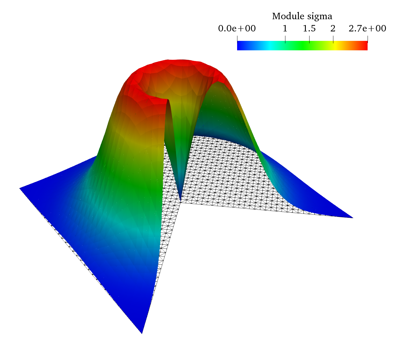
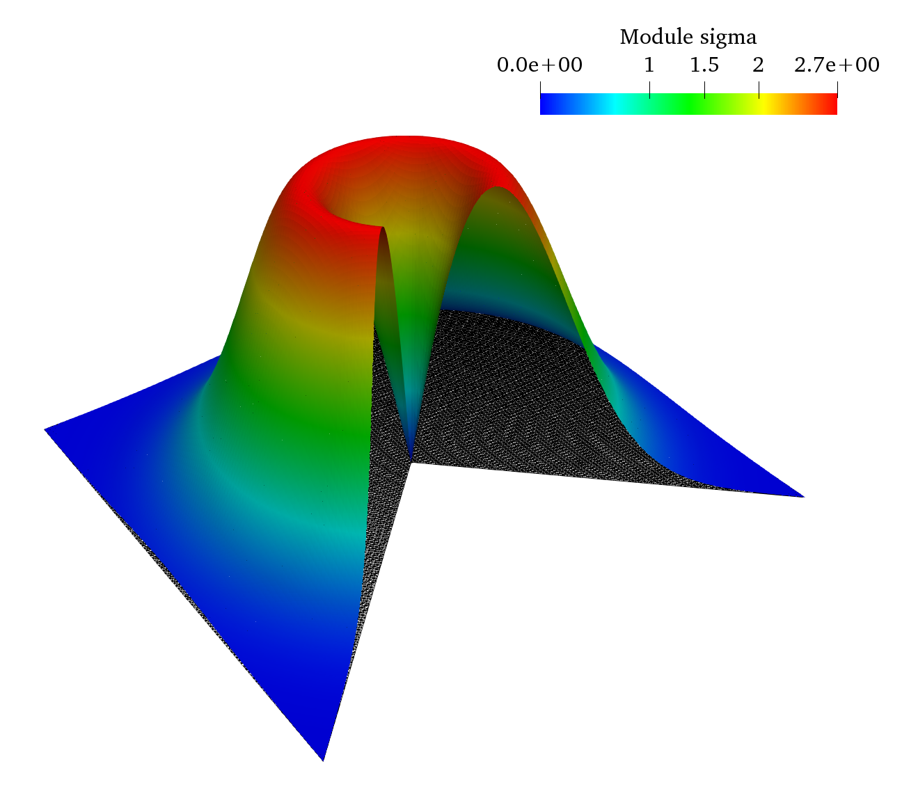
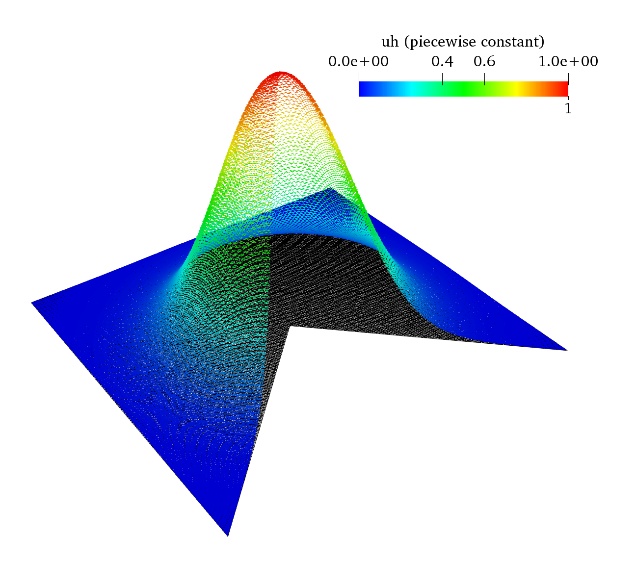
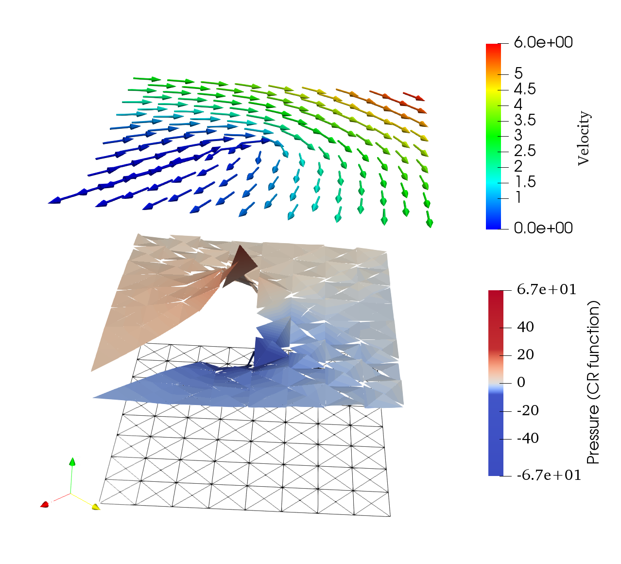
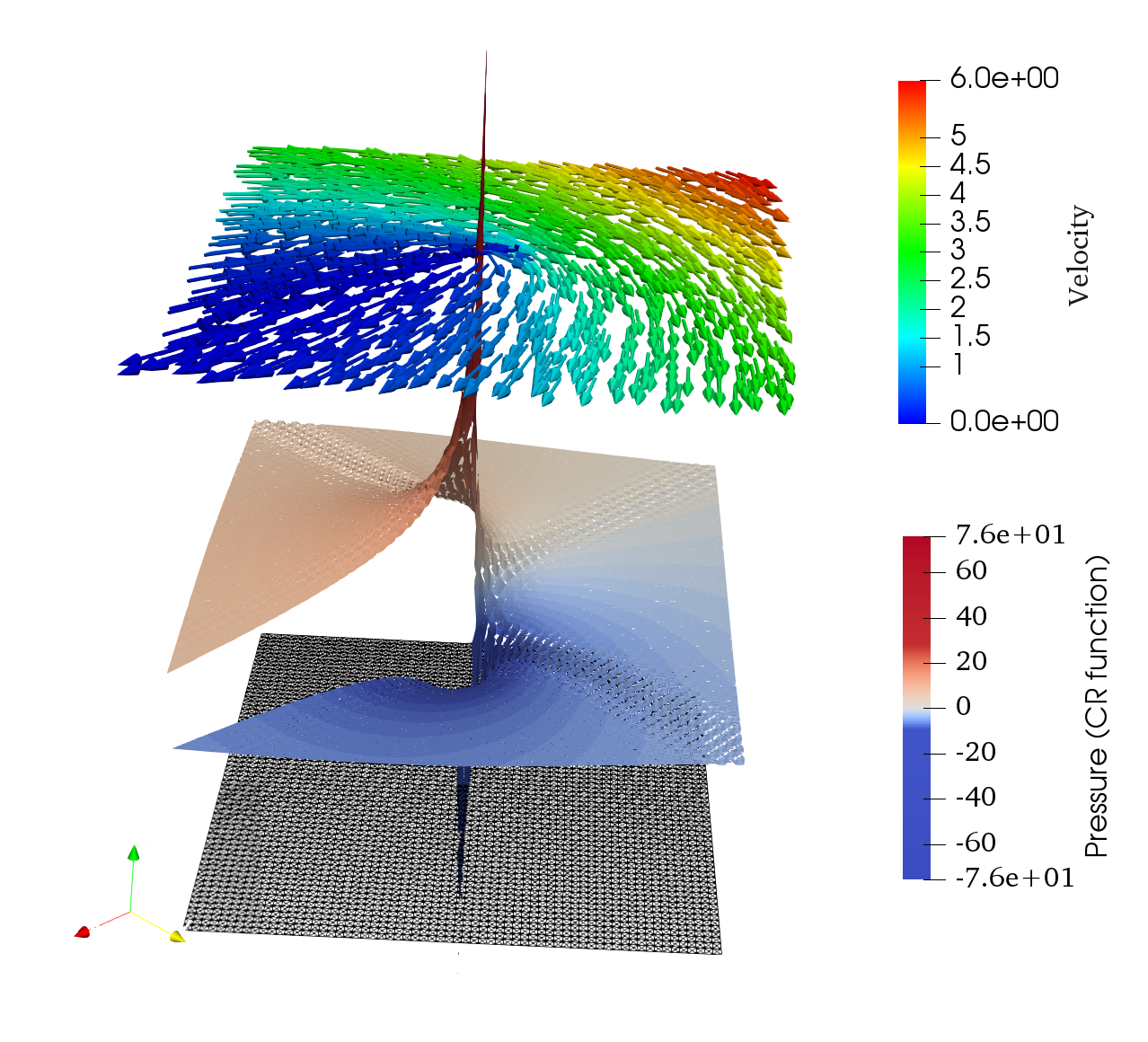
where denote polar coordinates. Note that is the solution of the elliptic equation in and that (we ignore the ). Figure 3 shows the discrete solution (piecewise constant) and the module of (module of a CR field) at iteration 6, respectively. We appreciate some small oscillations in the second picture, due to the singularity, but this does not affect the rates reported in Table 2. We omit the error, because it is almost zero ( is constant). Since at the reentrant corner, we expect (and see) the rate for the -error of The jump terms converge faster and the -error of converges with the optimal rate
| iter | DOFs | EOC | EOC | EOC | |||
|---|---|---|---|---|---|---|---|
| 1 | 212 | 1.152 | 0.68 | 1.033 | 0.66 | 5.465 | 1.04 |
| 2 | 808 | 7.524 | 0.64 | 5.610 | 0.91 | 2.750 | 1.03 |
| 3 | 3152 | 4.849 | 0.65 | 2.889 | 0.97 | 1.377 | 1.02 |
| 4 | 12448 | 3.092 | 0.66 | 1.461 | 0.99 | 6.886 | 1.01 |
| 5 | 49472 | 1.960 | 0.66 | 7.331 | 1.00 | 3.442 | 1.01 |
| 6 | 197248 | 1.238 | 0.66 | 3.669 | 1.00 | 1.721 | 1.00 |
| 7 | 787712 | 7.814 | 0.67 | 1.834 | 1.00 | 8.601 | 1.00 |
6.1.3. P3. Crack domain
Let be the crack domain shown in Figure 1 (right) with opening angle zero, and consider the following singular solution of (1.1):
| (6.3) |
where denote polar coordinates. Note that is the solution of the elliptic equation in The initial mesh is shown in Figure 1 (right). We emphasize that the DOFs on the line are different.
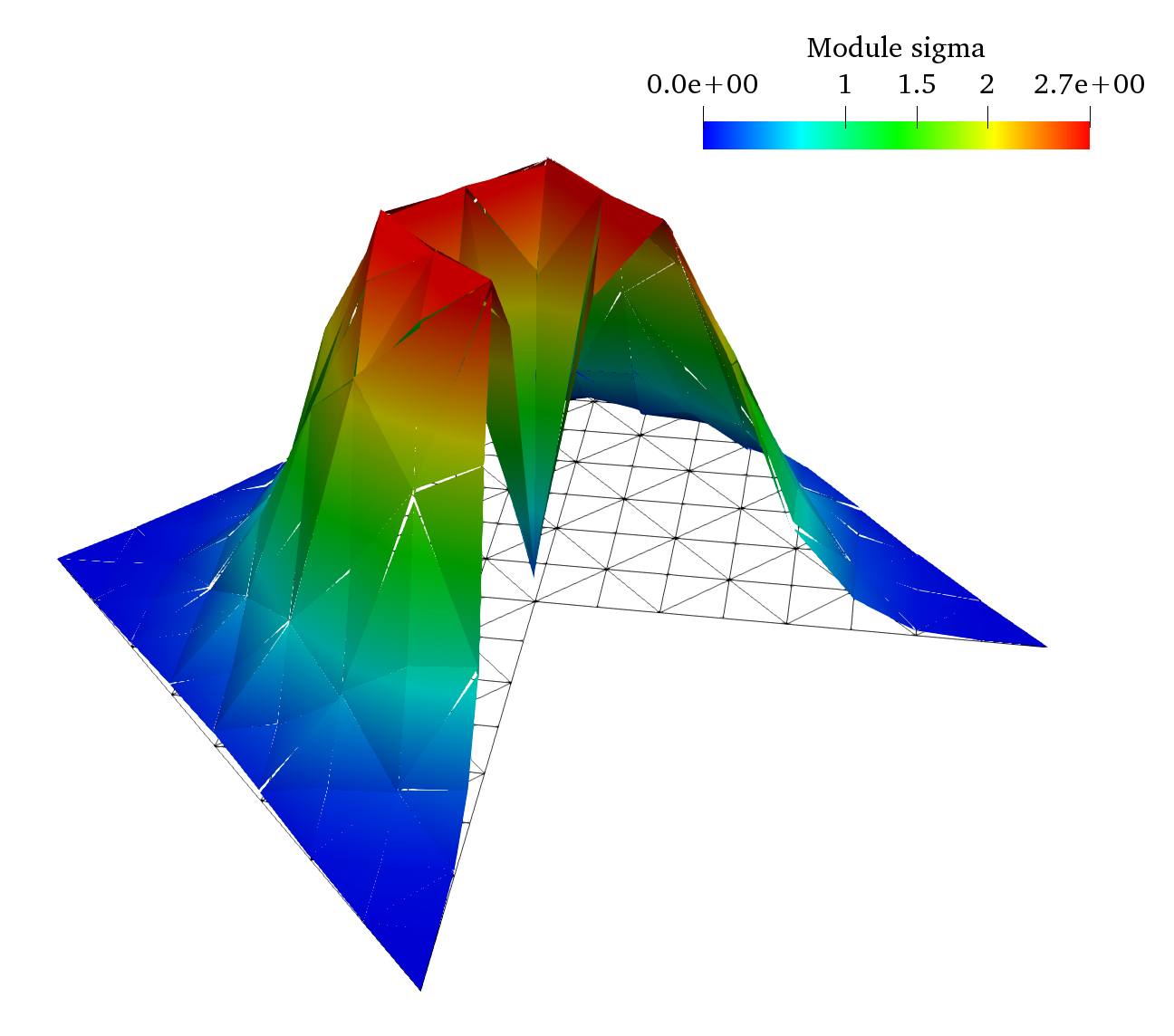
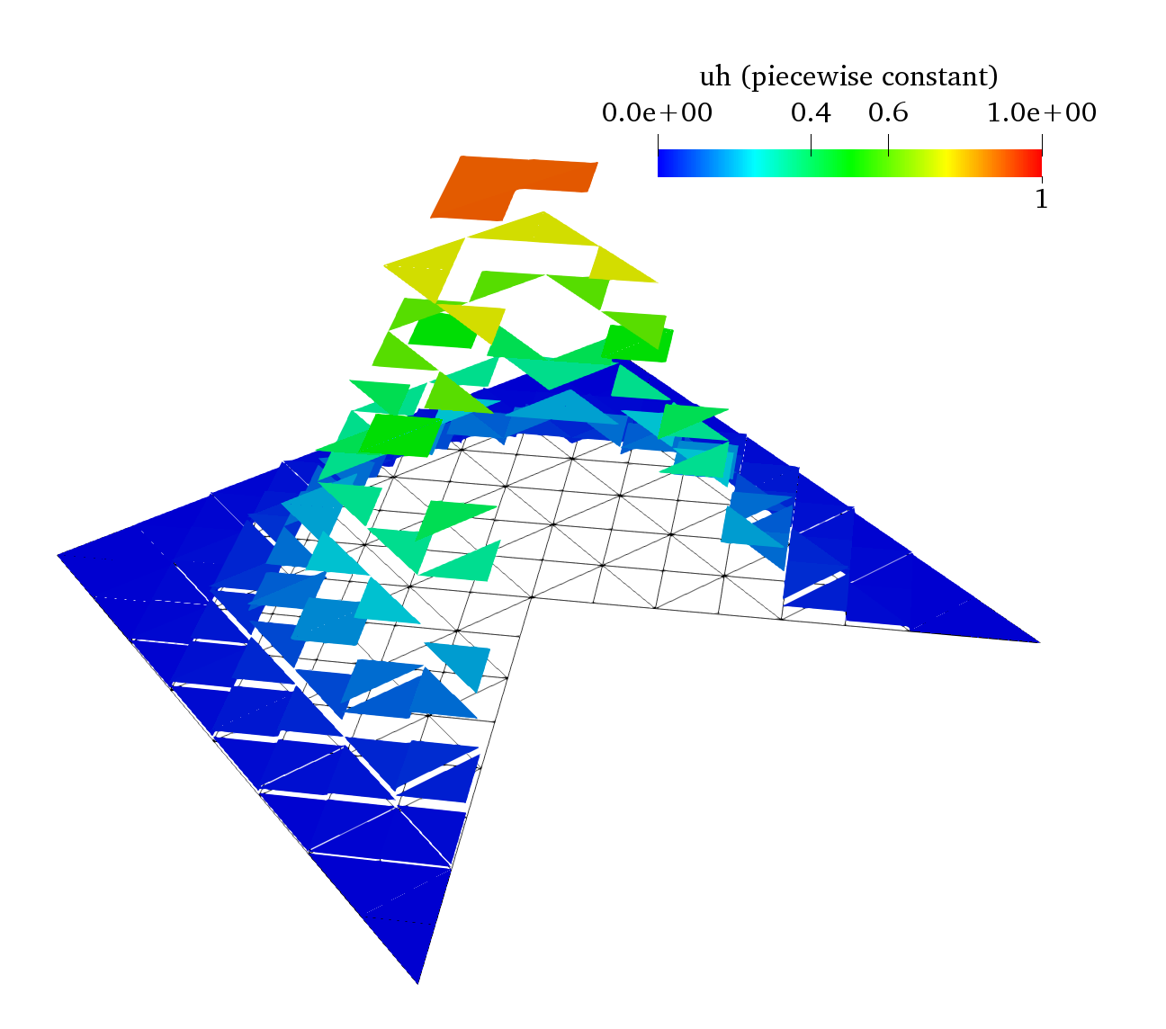
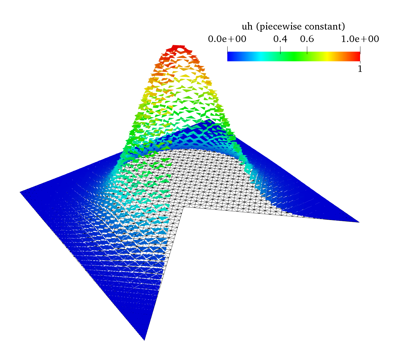
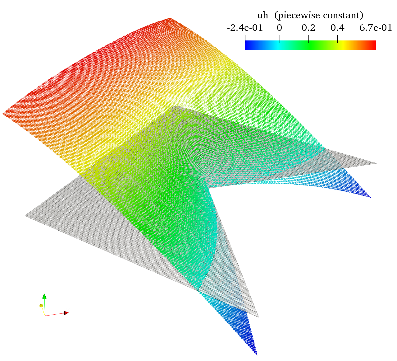
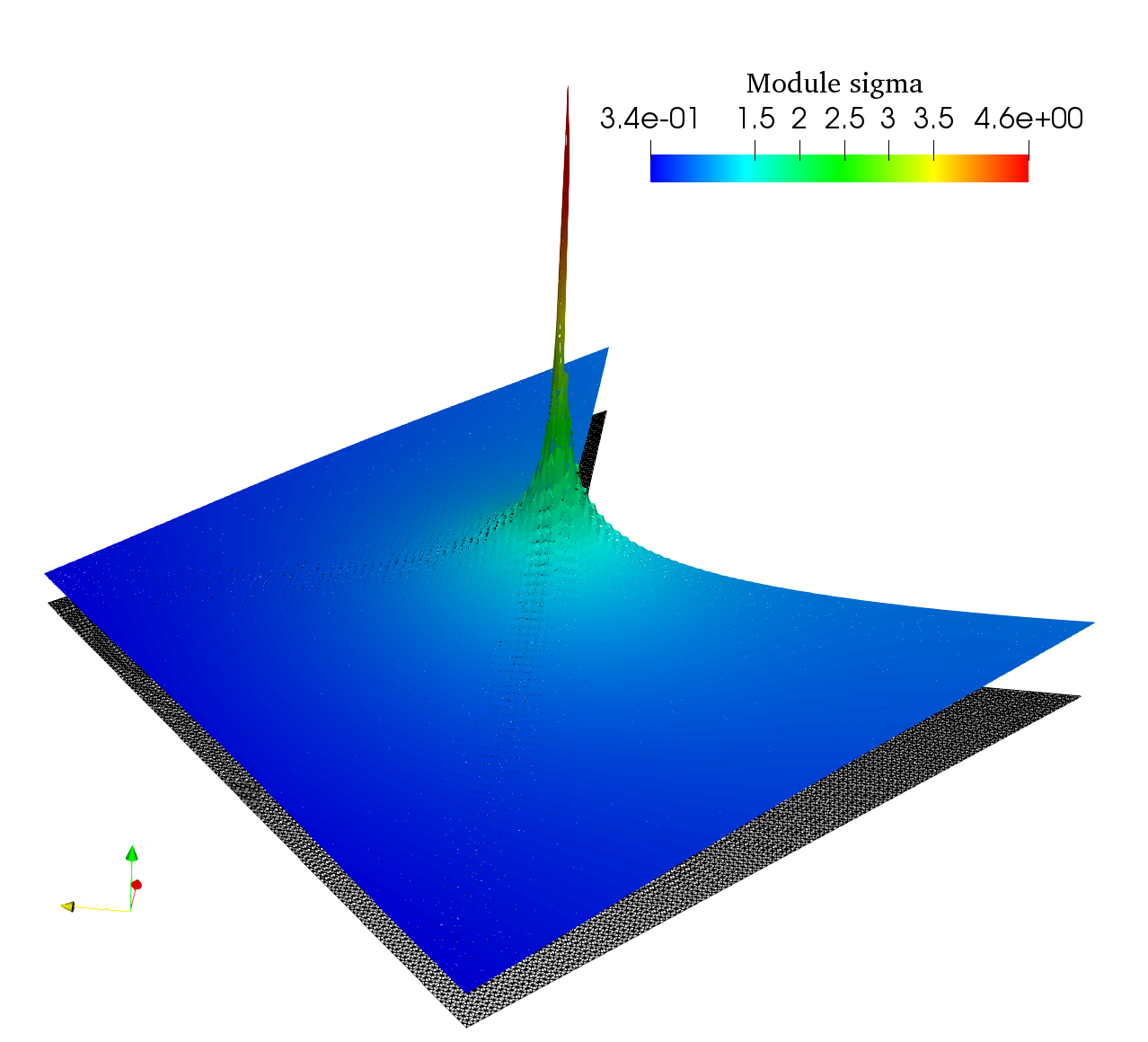
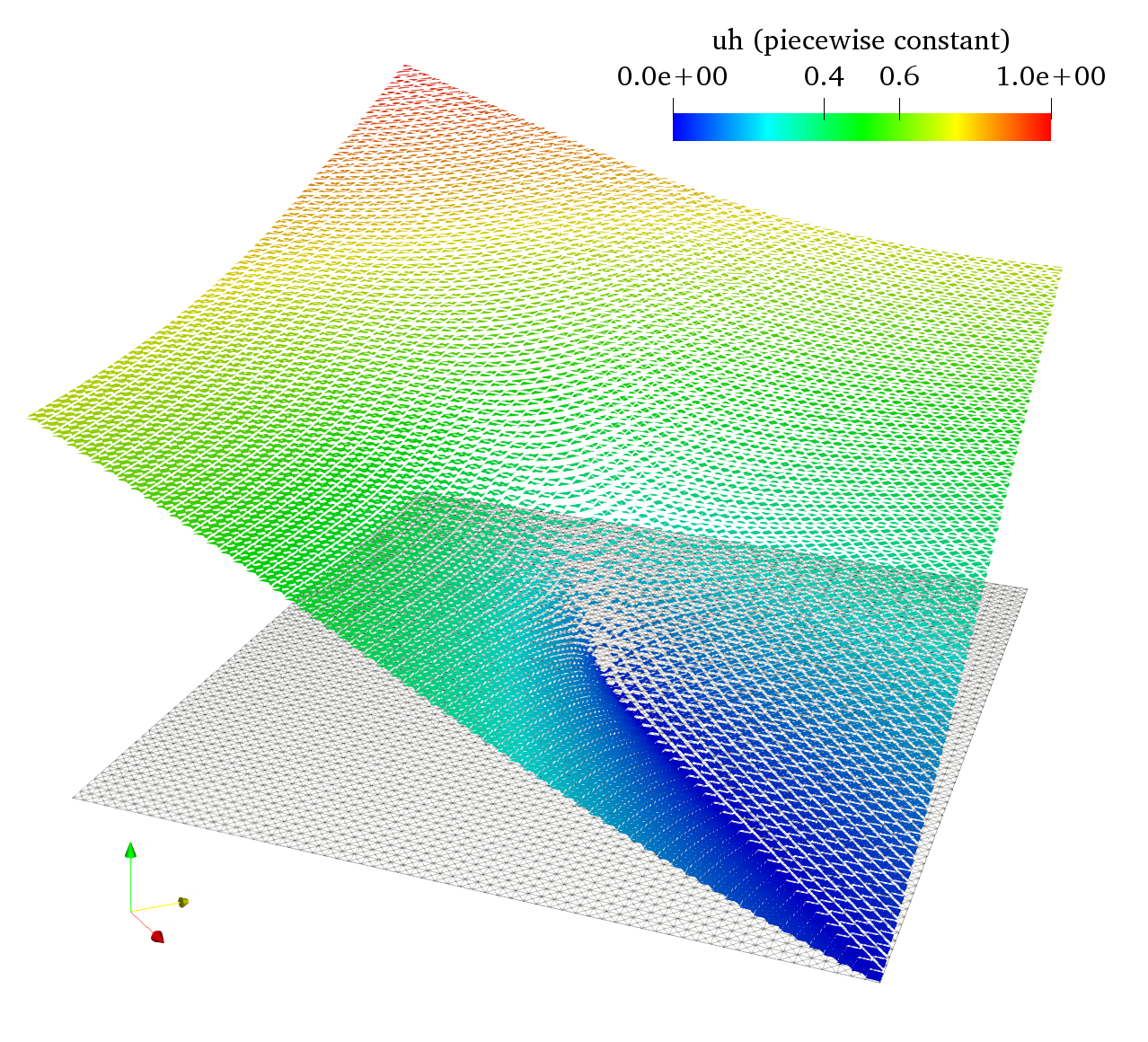
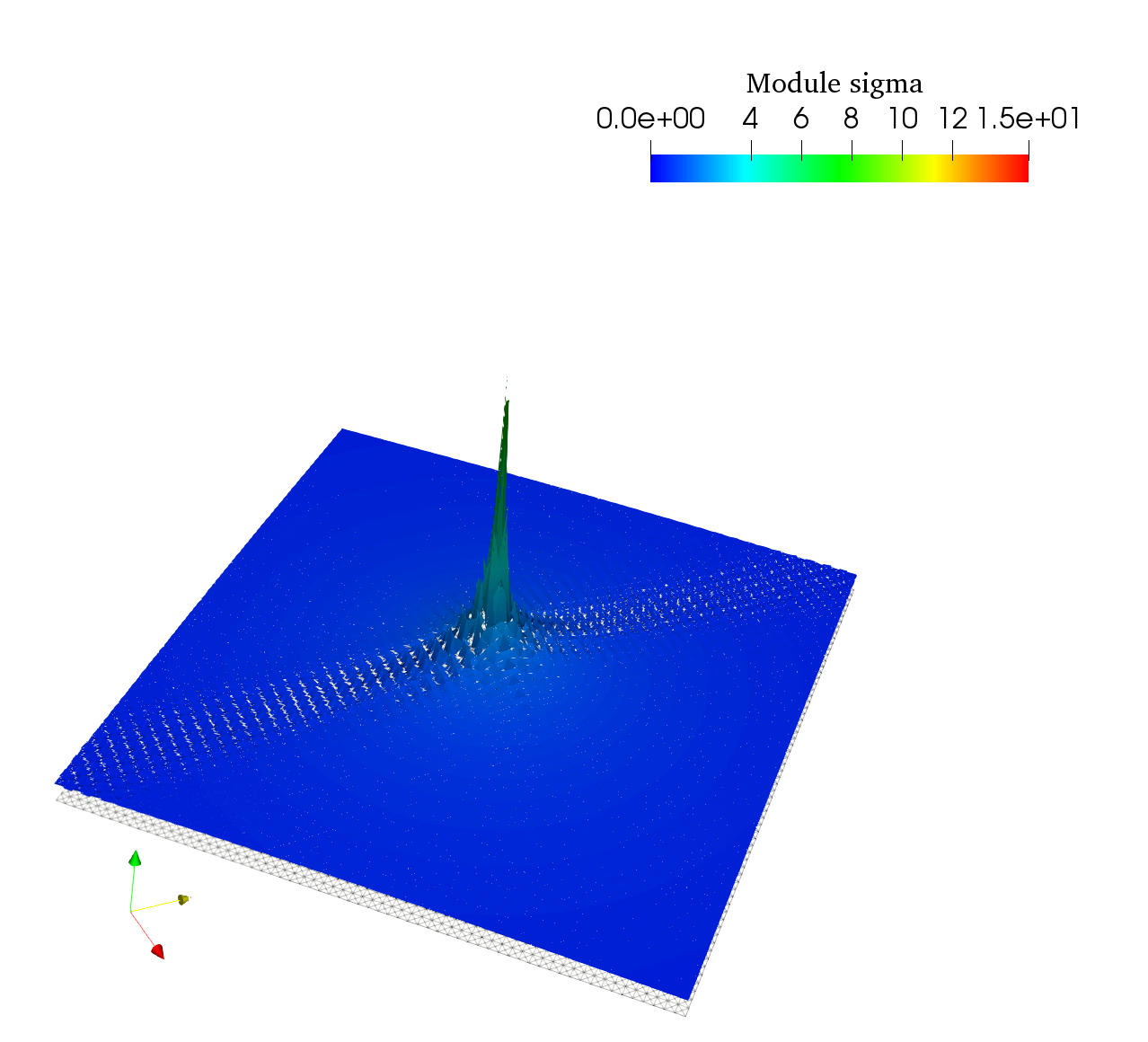
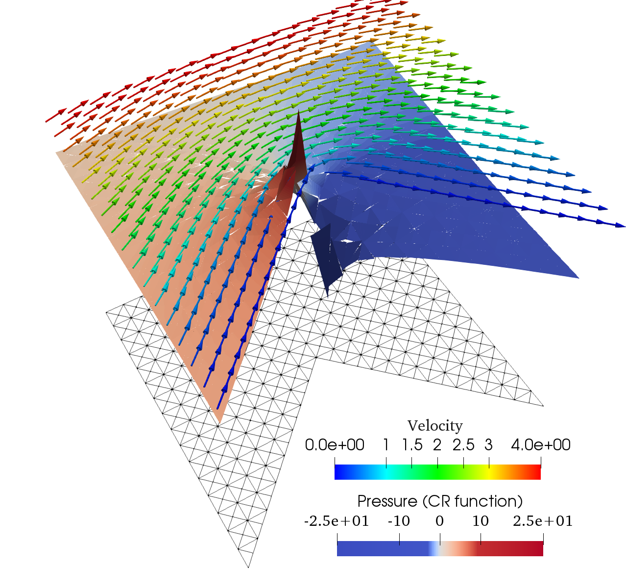
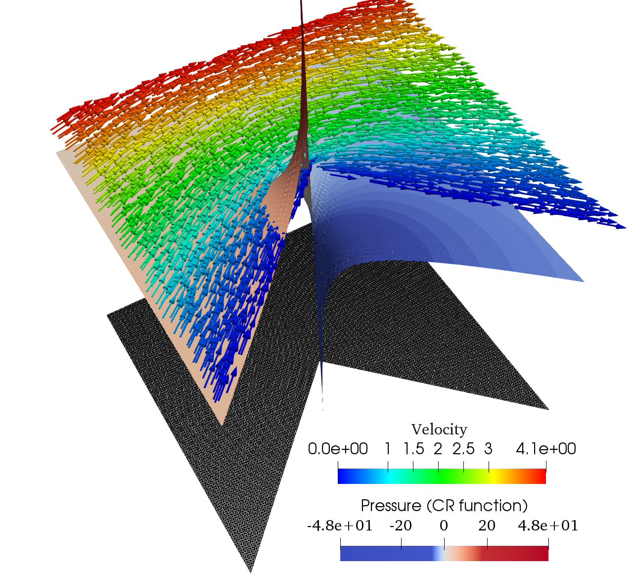
The error behaviours for this test are reported in Table 3. We observe optimal rates for the error of variable and the expected rate for the error of (according to the singularity). Finally, in Figure 4 we show the discrete solution and the module of at iteration 5.
| iter | DOFs | EOC | EOC | EOC | |||
|---|---|---|---|---|---|---|---|
| 0 | 76 | 3.410 | – | 1.968 | – | 1.290 | – |
| 1 | 280 | 2.648 | 0.39 | 1.353 | 0.57 | 6.817 | 0.98 |
| 2 | 1072 | 2.078 | 0.36 | 8.060 | 0.77 | 3.561 | 0.97 |
| 3 | 4192 | 1.581 | 0.40 | 4.592 | 0.82 | 1.833 | 0.97 |
| 4 | 16576 | 1.176 | 0.43 | 2.602 | 0.83 | 9.344 | 0.98 |
| 5 | 65920 | 8.598 | 0.45 | 1.482 | 0.82 | 4.734 | 0.98 |
| 6 | 262912 | 6.222 | 0.47 | 8.505 | 0.80 | 2.389 | 0.99 |
| 7 | 1050112 | 4.470 | 0.48 | 4.921 | 0.79 | 1.202 | 0.99 |
6.2. Stokes problem
In order to impose the zero mean value condition for the trace of functions in the spaces we consider the equivalent problem (5.6), that was introduced in Section 5.2. We recall that from definition of pseudostress the pressure can be recovered as: This identity allows us to analyze the pressure error, since
6.2.1. S1. Smooth solution
This example is motivated by the two-dimensional analytical solution of the Navier-Stokes equations derived by Kovasznay in [16], where we consider and:
| (6.4) |
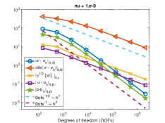
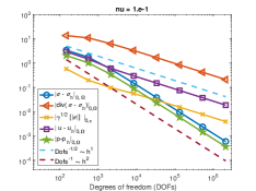
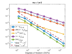
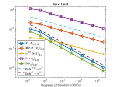
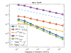
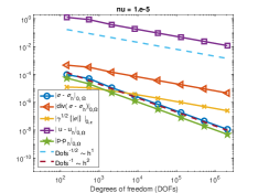
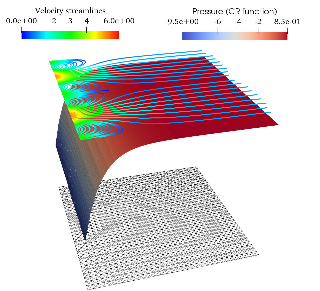
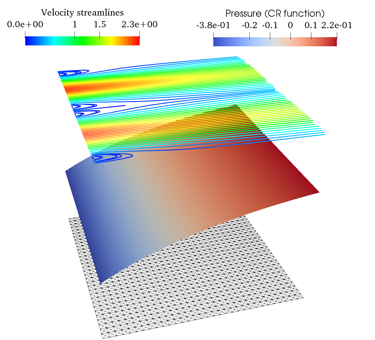
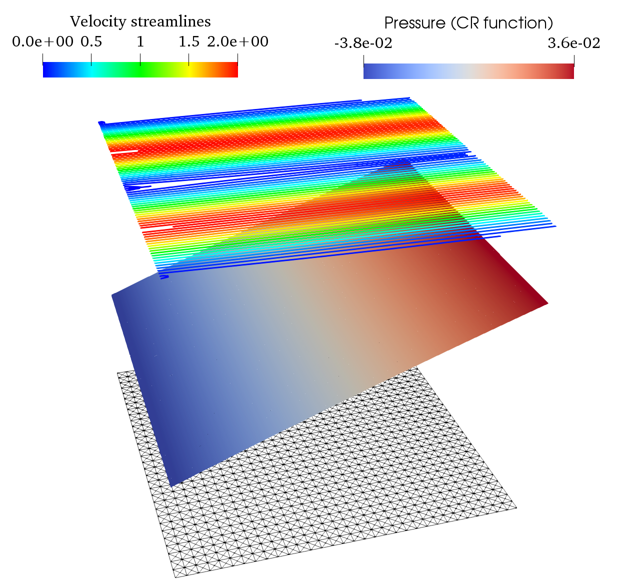
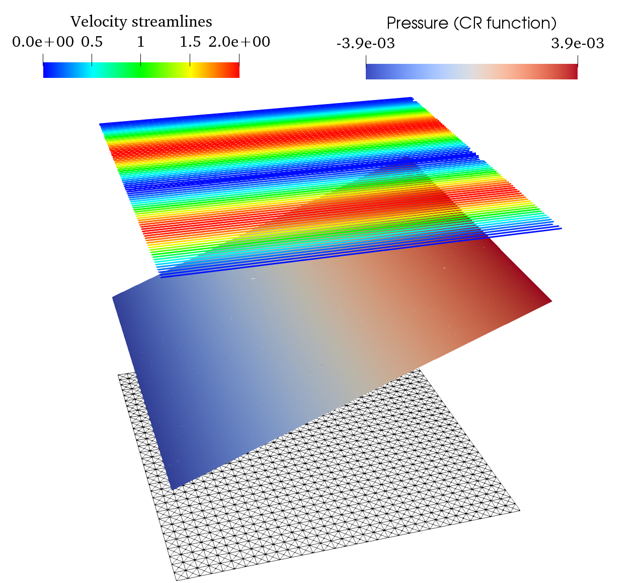
with the parameter given by: In order to test the robustness of our scheme, we solve the problem for different values of the viscosity, ranging from to Figure 5 shows the decay of the errors versus the DOFs. The convergence rates confirm the theory (Theorem 5.5) in all cases, that is, independent of the value of the viscosity we at least have linear convergence. We remark that the pressure errors decay faster with rate
In Figure 6, we show the velocity stream lines and pressure at iteration 4, for the viscosity values analyzed. We do not appreciate any instability featured caused by a small viscosity.


6.2.2. S2. M-shaped domain
We now consider the singular solution of (5.1) proposed in [18, page 113]. Again, let be M-shaped domain shown in Figure 1(left), and take and Then, if denote the polar coordinates, we impose an appropriate boundary condition for so that:
| (6.5) |
where
| (6.6) |
Here, and the coefficient is the smallest positive solution of:
We emphasize that are singular functions, and at the origin and Table 4 gives the individual errors and the corresponding rates. Again, we omit the divergence error because its size is close to the rounding unit.
As in the Poisson problem, we note that the jump and the -error of decay with rate The error of decay according to the regularity of the exact solution. Figure 7 show the velocity and pressure at iteration 3 and 6. We observe some oscillations in the first steps that diminish later as the mesh is refined.
| iter | DOFs | EOC | EOC | EOC | EOC | ||||
|---|---|---|---|---|---|---|---|---|---|
| 0 | 117 | 3.995 | – | 1.002 | – | 6.341 | – | 2.612 | – |
| 1 | 425 | 2.781 | 0.56 | 6.451 | 0.68 | 3.377 | 0.98 | 1.769 | 0.60 |
| 2 | 1617 | 1.851 | 0.61 | 3.515 | 0.91 | 1.725 | 1.01 | 1.145 | 0.65 |
| 3 | 6305 | 1.232 | 0.60 | 1.815 | 0.97 | 8.677 | 1.01 | 7.476 | 0.63 |
| 4 | 24897 | 8.289 | 0.58 | 9.194 | 0.99 | 4.341 | 1.01 | 4.967 | 0.60 |
| 5 | 98945 | 5.622 | 0.56 | 4.618 | 1.00 | 2.168 | 1.01 | 3.346 | 0.57 |
| 6 | 394497 | 3.833 | 0.55 | 2.312 | 1.00 | 1.082 | 1.00 | 2.273 | 0.56 |
| 7 | 1575425 | 2.620 | 0.55 | 1.155 | 1.00 | 5.406 | 1.00 | 1.551 | 0.55 |
6.2.3. S3. Crack domain
This last example is taken from [18, page 113]. We replicate the previous example on the crack domain, Figure 1(right) with given by (6.5) and
| (6.7) |
Table 5 reports the error decay. Again, we leave out the divergence error as it is close to the rounding unit. Although, this example is not covered by our theory, we obtain results equivalent to those in Section 6.1.3. We remark that the observed rates for the errors in and are slightly better than the expected value Finally, Figure 8 shows the velocity-field and pressure at iteration 2 and 5.
| iter | DOFs | EOC | EOC | EOC | EOC | ||||
|---|---|---|---|---|---|---|---|---|---|
| 0 | 153 | 9.801 | – | 1.218 | – | 8.093 | – | 6.657 | – |
| 1 | 561 | 8.096 | 0.29 | 8.714 | 0.52 | 4.669 | 0.85 | 5.449 | 0.31 |
| 2 | 2145 | 5.685 | 0.53 | 5.362 | 0.72 | 2.580 | 0.88 | 3.744 | 0.56 |
| 3 | 8385 | 3.750 | 0.61 | 3.107 | 0.80 | 1.363 | 0.94 | 2.395 | 0.66 |
| 4 | 33153 | 2.464 | 0.61 | 1.772 | 0.82 | 7.034 | 0.96 | 1.520 | 0.66 |
| 5 | 131841 | 1.649 | 0.58 | 1.008 | 0.82 | 3.584 | 0.98 | 9.861 | 0.63 |
| 6 | 525825 | 1.128 | 0.55 | 5.766 | 0.81 | 1.813 | 0.99 | 6.591 | 0.58 |
| 7 | 2100225 | 7.844 | 0.53 | 3.320 | 0.80 | 9.133 | 0.99 | 4.514 | 0.55 |
7. Final comments and conclusions
We developed an a priori error analysis for a low-order non-conforming method applied to the dual-mixed variational formulation of the Stokes and Poisson problem, and thus also for Darcy flow. Our a priori error estimates were established using Crouzeix-Raviart elements to approximate the and piecewise constants to approximate We proved a priori estimates for smooth solutions. Low regularity and a posteriori estimates are part of a forthcoming paper. However, the divergence error was proven to converge optimally for any regularity. The experimental approximation errors of our non-conforming scheme improve those of the conforming Raviart-Thomas approach.
Finally, an advantage of this approach over the one with Raviart-Thomas elements, is that, the CR-element is defined component-wise and not vector-wise. In fact, this leaves more flexibility for a symmetry restriction when dealing with elasticity equations, which is much more difficult to achieve with the Raviart-Thomas element. In particular for the lowest order Raviart-Thomas pair, this could only be done for a tensor with constant entries. We therefore, intent to extend the CR-element to the elasticity problem in a separate paper.
Acknowledgement
We are grateful to Erik Burman for providing us with the reference [10].
References
- [1] G. Acosta and R. G. Durán, The maximum angle condition for mixed and nonconforming elements: application to the Stokes equations, SIAM J. Numer. Anal., 37 (1999), pp. 18–36 (electronic).
- [2] D. Arnold, F. Brezzi, B. Cockburn, and L. Marini, Unified analysis of discontinuous Galerkin methods for elliptic problems, SIAM Journal on Numerical Analysis, 39 (2001), pp. 1749–1779.
- [3] T. Barrios and R. Bustinza, An augmented discontinuous Galerkin method for elliptic problems, Comptes Rendus Mathematique, 344 (2007), pp. 53–58.
- [4] , A priori and a posteriori error analyses of an augmented discontinuous Galerkin formulation, IMA Journal of Numerical Analysis, 30, 4 (2010), pp. 987–1008.
- [5] , A posteriori error analysis of an augmented discontinuous formulation for Darcy flow, Numerische Mathematik, 120 (2012), pp. 231–269.
- [6] T. P. Barrios and R. Bustinza, An a-priori error analysis for discontinuous lagrangian finite elements applied to nonconforming dual-mixed formulations: Poisson and stokes problems, Electron. Trans. Numer. Anal., 52 (2020), pp. 455–479.
- [7] T. P. Barrios, R. Bustinza, and F. Sánchez, Analysis of dG approximations for Stokes problem based on velocity-pseudostress formulation, Numerical Methods for Partial Differential Equations, 33, 5 (2017), pp. 1540–1564.
- [8] M. Bebendorf, A note on the poincaré inequality for convex domains, Zeitschrift Fur Analysis Und Ihre Anwendungen - Z ANAL ANWEND, 22 (2003), pp. 751–756.
- [9] S. C. Brenner, Forty Years of the Crouzeix–Raviart element, Numerical Methods for Partial Differential Equations, 31 (2015), pp. 367–396.
- [10] E. Burman and P. Hansbo, Stabilized crouzeix-raviart element for the darcy-stokes problem, Numerical Methods for Partial Differential Equations, 21 (2005), pp. 986–997.
- [11] Z. Cai, C. Tong, P. Vassilevski, and C. Wang, Mixed finite element methods for incompressible flow: Stationary Stokes equations, Numerical Methods for Partial Diferential Equations, 26 (2010), pp. 957–978.
- [12] P. G. Ciarlet, The finite element method for elliptic problems, North-Holland Publishing Co., Amsterdam, 1978.
- [13] M. Crouzeix and P.-A. Raviart, Conforming and nonconforming finite element methods for solving the stationary Stokes equations. I, Rev. Française Automat. Informat. Recherche Opérationnelle Sér. Rouge, 7 (1973), pp. 33–75.
- [14] G. Gatica and F. Sayas, A note on the local approximation properties of piecewise polynomials with applications to LDG methods, Complex Variables and Elliptic Equations, 51,2 (2006), pp. 109–117.
- [15] V. Girault and P.-A. Raviart, Finite Element Methods for Navier Stokes Equations, Springer, Berlin, 1986.
- [16] L. Kovasznay, Laminar flow behind a two-dimensional grid, Mathematical Proceedings of the Cambridge Philosophical Society, 44 (1948), pp. 58–62.
- [17] A. Schmidt and K. Siebert, Design of Adaptive Finite Element Software, Lecture Notes in Computational Science and Engineering, 42, Springer-Verlag Berlin Heidelberg, 2005.
- [18] R. Verfürth, A review of a posteriori error estimation and adaptive mesh-refinement techniques, Advances in numerical mathematics, Wiley-Teubner, 1996.
- [19] T. Warburton and J. S. Hesthaven, On the constants in -finite element trace inverse inequalities, Comput. Methods Appl. Mech. Engrg., 192 (2003), pp. 2765–2773.