Machine Learning Optimized Search
for the $Z^{\prime}$ from $U(1)_{L_{\mu}-L_{\tau}}$ at the LHC

Manuel Drees¹, Meng Shi¹, Zhongyi Zhang^1,2,3

¹Bethe Center for Theoretical Physics,
Bonn University, 53115 Bonn, Germany
²Institute for Mathematics, Astrophysics and Particle Physics
Radboud University, 6525 AJ Nijmegen, Netherlands
³Nikhef, Science Park 105, 1098 XG Amsterdam, Netherlands

Extending the Standard Model (SM) by a $U(1)_{L_{\mu}-L_{\tau}}$ group gives potentially significant new contributions to $g_{\mu}-2$, allows the construction of realistic neutrino mass matrices, incorporates lepton universality violation, and offers an anomaly–free mediator for a Dark Matter (DM) sector. In a recent analysis we showed that published LHC searches are not very sensitive to this model. Here we apply several Machine Learning (ML) algorithms in order to distinguish this model from the SM using simulated LHC data. In particular, we optimize the $3\mu$–signal, which has a considerably larger cross section than the $4\mu$–signal. Furthermore, since the $2$–muon plus missing $E_{T}$ final state gets contributions from diagrams involving DM particles, we optimize it as well. We find greatly improved sensitivity, which already for $36$ fb^-1 of data exceeds the combination of published LHC and non–LHC results. We also emphasize the usefulness of Boosted Decision Trees which, unlike Neural Networks, easily allow to extract additional information from the data which directly connect to the theoretical model through feature importance. The same scheme could be used to analyze other models.

1 Introduction

Extending the Standard Model (SM) by a gauged $U(1)_{L_{\mu}-L_{\tau}}$ group [1] does not introduce new gauge anomalies even if we stick to the SM fermion content, but leads to potentially sizable positive contributions to the anomalous magnetic moment of the muon ($g_{\mu}-2$), whose SM prediction [2] is too low by about $4.2\,\sigma$ [3]. Once right–handed neutrinos are introduced it also allows the construction of realistic neutrino mass matrices [4, 5], and it can be used to construct realistic models of particle Dark Matter (DM) [6]. Moreover, since the model does not introduce extra couplings of the electron, it avoids the strong constraints from $e^{+}e^{-}\rightarrow\mu^{+}\mu^{-}$ or $e^{+}e^{-}\rightarrow\tau^{+}\tau^{-}$ in $e^{+}e^{-}$ collision experiments.

In a previous work [7] we studied to what extent published LHC analyses can be used to constrain this model through the production and decay of the new $Z^{\prime}$ gauge boson. We also allowed for the existence of a DM particle charged under $U(1)_{L_{\mu}-L_{\tau}}$, either a complex scalar ($\phi_{\rm DM}$) or Dirac spinor ($\chi_{\rm DM}$). We found that for most values of the mass $m_{Z^{\prime}}$ of the new gauge boson, published LHC analyses impose a weaker bound on the new gauge coupling $g_{\mu\tau}$ than non–LHC experiments, the latter being dominated by searches for low–mass $Z^{\prime}$ at BaBar [8] as well as neutrino “trident” experiments [9, 10, 11]. Only for $10\ {\rm GeV}\leq m_{Z^{\prime}}\leq 60$ GeV does the best bound on $g_{\mu\tau}$ come from the LHC, thanks to a dedicated search by CMS [12] in the four muon final state.

The sensitivity of LHC data can clearly be improved by applying selection rules that have been optimized to search for this specific $Z^{\prime}$ boson. In our previous analysis [7] we had seen that final states with muons always have better sensitivity than otherwise equivalent final states with hadronically decaying $\tau$ leptons. Moreover, since the cross section for producing $\mu\nu_{\mu}Z^{\prime}$ final states is considerably larger than that for $\mu^{+}\mu^{-}Z^{\prime}$ production, the best sensitivity for $Z^{\prime}$ searches at the LHC is expected in the $3\mu+\not{E}_{T}$ final state, where $\not{E}_{T}$ stands for missing transverse energy. An exception may occur if the invisible width of the $Z^{\prime}$ is very large. The latter depends on the mass and charge of the DM particle, and can be probed in the $\mu^{+}\mu^{-}+\not{E}_{T}$ final state. In this paper we therefore focus on these final states.

Since the new contribution to the $3\mu+\not{E}_{T}$ signal will be dominated by the production and decay of nearly on–shell $Z^{\prime}$ bosons, we design a simple set of cuts, assuming that one can guess the value of $m_{Z^{\prime}}$ from the di–muon invariant mass distribution; this is essentially a classical “bump hunt”. In addition, we develop and compare a variety of machine learning (ML) methods. Our goal is to find a single classifier that has good sensitivity over a wide range of $Z^{\prime}$ masses, rather than devising dedicated searches for each value of $m_{Z^{\prime}}$. Moreover, at least initially we consider a large number of input variables, including both low–level features (the $4-$momenta of the final state objects) and higher–level features (e.g. invariant masses of pairs of final state objects); the latter are taken from published experimental analyses of multi–lepton final states.

We find that, after sufficient training, a fully connected deep neural net (NN) and a gradient boosted decision tree (GBDT) outperformed the simple bump hunt. Moreover, the GBDT allowed to identify the most important input features, which helps to extract physical information from the ML algorithm; in contrast, the NN is basically a “black box”. The information of the original GBDT on feature importance also led us to devise simpler classifiers, for both NN and GBDT, with significantly fewer input quantities but almost equally good performance. Performing both a NN and a GBDT analysis therefore guarantees excellent sensitivity of the $Z^{\prime}$ search, and physical insight in the important kinematical features of the signal.

The remainder of this article is organized as follows. In Section 2 we briefly describe the SM extended with the $U(1)_{L_{\mu}-L_{\tau}}$, focusing on the parts of the Lagrangian that can be probed in searches for $3\mu+\not{E}_{T}$ and $\mu^{+}\mu^{-}+\not{E}_{T}$ final states at the LHC, and the corresponding Feynman diagrams. In Section 3, we describe the data set and training process for ML based classifiers. In Section 4, we discuss the results from this new approach, while Section 5 contains a summary of our study and some conclusions. The Appendices contain a brief tutorial for the machine learning techniques we used as well as additional figures.

2 Model, Lagrangian, and Signal

2.1 The Simplified Model

Extending the SM gauge group of $SU(3)_{c}\otimes SU(2)_{L}\otimes U(1)_{Y}$ by a local $U(1)_{L_{\mu}-L_{\tau}}$ symmetry requires the introduction of a new gauge boson $Z^{\prime}$, which can also be a mediator connecting SM to DM particles; the corresponding field strength tensor is $\mathcal{Z}^{\prime}_{\mu\nu}\equiv\partial_{\mu}Z^{\prime}_{\nu}-\partial_{\nu}Z^{\prime}_{\mu}$, while the covariant derivative instead of the normal partial derivative can be used to describe the interactions, i.e. $\partial_{\mu}\rightarrow D_{\mu}=\partial_{\mu}-ig_{\mu\tau}q_{\mu\tau}Z^{\prime}_{\mu}$, where $g_{\mu\tau}$ is the new gauge coupling and $q_{\mu\tau}$ the corresponding $L_{\mu}-L_{\tau}$ charge. The model may contain a complex scalar DM particle $\phi_{\rm DM}$ or a spinor DM particle $\chi_{\rm DM}$, which are singlets under the gauge groups of the SM but carry $L_{\mu}-L_{\tau}$ charge $q_{\rm DM}$. The DM particle affects LHC physics basically only through $Z^{\prime}$ decays into invisible final states. As long as we keep the mass and charge of the DM particle as free parameters, we can therefore fix its spin without loss of generality. For definiteness we consider the scalar DM particle here.

The kinetic term of the massive mediator $Z^{\prime}$ is $\mathcal{L}_{Z^{\prime}}=-\frac{1}{4}\mathcal{Z}^{\prime}_{\mu\nu}\mathcal{Z}^{\prime\mu\nu}$, while the kinetic term of DM particle is $(D^{\mu}\phi_{\rm DM})^{*}D_{\mu}\phi_{\rm DM}$. We are interested in a massive $Z^{\prime}$. Since we do not treat higher order corrections due to the new interaction, the way the $Z^{\prime}$ mass is generated is not important for us. One can certainly design a simple Higgs sector which breaks $U(1)_{L_{\mu}-L_{\tau}}$ spontaneously without introducing new physical particles that can be produced in on–shell $Z^{\prime}$ decays. This symmetry breaking, and/or the vacuum expectation value of the SM Higgs field, can contribute to the mass of the DM particle, in addition to a gauge invariant mass term; however, for us only the total mass of this particle is relevant, which is a free parameter. Finally, in order to produce a realistic neutrino mass matrix through a type–I see–saw mechanism one can introduce three SM singlet right–handed neutrinos [4]. We will assume that all new fermions that carry $L_{\mu}-L_{\tau}$ charge have mass above $m_{Z^{\prime}}/2$.

The parts of the Lagrangian relevant for our analysis can thus be written as

$$\mathcal{L}_{\textrm{new}} = (D_{\mu}\phi_{\textrm{DM}})^{*}D^{\mu}\phi_{\textrm{DM}}-m_{\textrm{DM}}^{2}\phi^{*}_{\textrm{DM}}\phi_{\textrm{DM}}-\frac{1}{4}\mathcal{Z}^{\prime}_{\mu\nu}\mathcal{Z}^{\prime\mu\nu}+\frac{1}{2}m_{Z^{\prime}}^{2}Z^{\prime\mu}Z^{\prime}_{\mu}$$

$$+ g_{\mu\tau}(\bar{\mu}\not{Z}^{\prime}\mu+\bar{\nu}_{\mu}\not{Z}^{\prime}\nu_{\mu}-\bar{\tau}\not{Z}^{\prime}\tau-\bar{\nu}_{\tau}\not{Z}^{\prime}\nu_{\tau}).$$

The LHC signals we consider stem from the production and decay of (nearly) on–shell $Z^{\prime}$ bosons. The above assumptions about the particle spectrum imply that at leading order the $Z^{\prime}$ can only decay into second or third generation leptons, and possibly into DM particles. The corresponding partial widths are

$$\Gamma(Z^{\prime}\rightarrow l^{+}l^{-})=\frac{g_{\mu\tau}^{2}m_{Z^{\prime}}}{12\pi}\sqrt{1-4z_{l}}(1+2z_{l})\,,\ \ {\textrm{for}}\ l=\mu,\,\tau;$$ (2)

$$\Gamma(Z^{\prime}\rightarrow\phi_{\textrm{DM}}\bar{\phi}_{\textrm{DM}})=\frac{q^{2}_{\textrm{DM}}g^{2}_{\mu\tau}m_{Z^{\prime}}}{48\pi}(1-4z_{\textrm{DM}})^{3/2}\,,$$ (3)

where $z_{X}\equiv m_{X}^{2}/m_{Z^{\prime}}^{2}$ and $\bar{\phi}$ stands for a DM antiparticle. The partial width for $Z^{\prime}$ decays into one flavor ($\mu$ or $\tau$) of neutrino is half of that given in eq.(2), since only the left–handed neutrinos contribute. Here we are interested in scenarios with $m_{Z^{\prime}}\geq 10$ GeV; even lighter $Z^{\prime}$ can probably be better probed through $l^{+}l^{-}Z^{\prime}$ production at low–energy $e^{+}e^{-}$ colliders. If $m_{\rm DM}\geq m_{Z^{\prime}}/2$ or $q^{2}_{\rm DM}\ll 1$ we then have ${\rm Br}(Z^{\prime}\rightarrow\mu^{+}\mu^{-})\simeq{\rm Br}(Z^{\prime}\rightarrow\tau^{+}\tau^{-})\simeq{\rm Br}(Z^{\prime}\rightarrow{\rm invisible})\simeq 1/3$; such scenarios will be investigated in Chapter 4.1. On the other hand, if $m_{\rm DM}<m_{Z^{\prime}}/2$ the invisible branching ratio can be enhanced; this will be analyzed in Chapter 4.2.

Our perturbative analysis will not be reliable if the new gauge coupling is very large. We therefore only consider scenarios where the total $Z^{\prime}$ width is smaller than $m_{Z^{\prime}}$, which implies

$$q^{2}_{\textrm{DM}}(1-4z_{\textrm{DM}})^{3/2}+4\sum_{l=\mu,\,\tau}\sqrt{1-4z_{l}}(1+2z_{l})+4<48\pi/g^{2}_{\mu\tau}\,.$$ (4)

This bound is always satisfied for $g_{\mu\tau}\leq 3$ and $q_{\textrm{DM}}\leq 2$.

2.2 Signals

Figure 1: Examples of Feynman diagrams for $pp\rightarrow Z^{\prime}\ell^{+}\ell^{-}$ (left), $pp\rightarrow Z^{\prime}\nu_{\ell}\bar{\nu}_{\ell}$ (center) and $pp\rightarrow Z^{\prime}\ell\nu_{\ell}$ (right); here $\ell$ stands for a $\mu$ or $\tau$ lepton. In the event generation, the $Z^{\prime}$ is allowed to be off–shell.

The signals we are interested in originate from the production of (real or virtual) $Z^{\prime}$ bosons [13, 14, 15]. Examples of the contributing Feynman diagrams are shown in Fig. 1: the $Z^{\prime}$ can be emitted off a $\mu^{+}\mu^{-}$ or $\tau^{+}\tau^{-}$ pair (left); off a second or third generation $\nu\bar{\nu}$ pair (middle); and off a $\mu\nu_{\mu}$ or $\tau\nu_{\tau}$ line (right). Our assumptions imply that the only visible particles that can be produced in $Z^{\prime}$ decays are muons and tau leptons. Invisible $Z^{\prime}$ decays in the left figure and visible $Z^{\prime}$ decays in the middle contribute to the $2\mu$ signal; recall that the former can receive contributions from $Z^{\prime}$ decays into DM particles. Visible $Z^{\prime}$ decays in the left diagram lead to $4\mu$ signal; the CMS analysis [12] investigated this final state for the case that all muons originate from the decay of an (almost) on–shell $Z$ boson, offering good sensitivity for $10\ {\rm GeV}\leq m_{Z^{\prime}}\leq 60$ GeV.

In the right figure, invisible $Z^{\prime}$ decays lead to single lepton final states, which we do not consider because of the very large SM background from the production of (possibly off–shell) leptonically decaying $W^{\pm}$ bosons. Visible $Z^{\prime}$ decays here lead to $3\mu$ signals. Note that this class of diagrams offers a significantly larger cross section (after summing over both possible charges) than those giving rise to $4\mu$ final states. In our previous work [7] we indeed found the best sensitivity for $3\mu$ final states, except for the mass range that can be probed in the decay of on–shell $Z$ bosons [12].

In the above discussion $\ell$ stands for a $\mu$ or $\tau$ lepton. The former are stable as far as the LHC experiments are concerned, and are straightforward to identify experimentally, if they are produced sufficiently centrally and with sufficient transverse momentum $p_{T}$ (the precise requirements will be given below). In contrast, tau leptons decay very quickly. $\tau\rightarrow\mu\nu_{\mu}\nu_{\tau}$ decays contribute another, softer, muon to the final state. $\tau\rightarrow e\nu_{e}\nu_{\tau}$ decays lead to qualitatively different final states, which come with their own sources of background. Since our $Z^{\prime}$ does not couple to electrons, replacing a muon (pair) in a multi–muon final state by an electron (pair) will greatly reduce the signal cross section, whereas the SM background, being essentially flavor universal, will remain the same; this therefore results in a final state with much worse signal to background ratio. Finally, $\tau$ leptons can decay into hadrons plus a $\nu_{\tau}$; however, these decays are not easy to identify experimentally, and suffer from considerably additional backgrounds. The upshot of this discussion is that we expect the best sensitivity in final states defined exclusively via the number of muons and missing $E_{T}$; indeed, this is what we saw in our previous study [7]. It should be noted that the $3\mu$ signal also receives a (small) contribution from the left diagram of Fig. 1 if at least two of the leptons are $\tau$’s, one of which decays into a muon while the others decay hadronically. Similarly, all three diagrams can contribute to the $2\mu$ final state.

In order to simulate the $2\mu$ and $3\mu$ backgrounds and signals at tree level we use MadGraph [16] to generate the process $pp\rightarrow m\mu+n\tau+(4-m-n)\not{p}$, where $\not{p}$ means neutrinos or DM, $m,n\geq 0$, and $3(2)\leq m+n\leq 4$, under the condition that only events with exactly two or exactly three muons in the final state are accepted. The signal contribution is defined by requiring at least (in practice, exactly) one $Z^{\prime}$ propagator in the Feynman diagram, as shown in Fig. 1. The backgrounds come from diagrams with two electroweak gauge bosons ($\gamma,W^{\pm}$ or $Z$). In addition to diagrams of the kind shown in Fig. 1 where the $Z^{\prime}$ is replaced by a virtual $\gamma$ or a $Z$ boson, there are also diagrams where both gauge bosons couple to the initial $q\bar{q}$ line.

Note that we do not generate background events where the muon result from the decay of heavy quarks. At the fully inclusive level these backgrounds are very large; in fact, generating a sufficient number of events where muons originate from charm or bottom decay is difficult with our computational resources. However, their physical characteristics are quite different from the signal events. By focusing on backgrounds with the same parton–level final state as the signal we concentrate on the probably most dangerous background, which is most difficult to discriminate from the signal. We will show that machine learning methods perform quite well in this task.

3 Machine Learning Based Methods

We use a gradient boosting decision tree (GBDT) and a deep learning neural network (NN) as tools to discriminate the possible $Z^{\prime}$ signals from the Standard Model background. The NN is less prone to be affected by the choice of input variables, called “features” in the following. In particular, it can perform well even with very basic features [17]. However, the inner workings of a NN are not easy to understand, it is basically a “black box”. On the other hand, a GBDT allows to determine the relative importance of various features, which helps to understand the physics of the final event selection.

Both the NN and the GBDT need to be trained. To that end we generated 1 million signal and 1 million background events for each of seven values of $m_{Z^{\prime}}$ ($10$, $50$, $100$, $200$, $300$, $400$, and $500$ GeV). The signal events were generated with $g_{\mu\tau}=1$ and $q_{\rm DM}=0$, so that $\Gamma_{Z^{\prime}}\simeq 0.08m_{Z^{\prime}}$, see eq.(2). We changed the random seed for the generation of background events, hence the final data we use for training are statistically independent. Note that we use a single GBDT and a single NN, trained on events for all values of $m_{Z^{\prime}}$, because we want to check how well the ML algorithms are able to understand the mixed data. Moreover, we expect that the performance of the signal classifiers trained in this manner will also be largely independent of the $Z^{\prime}$ width.

In our simulation, parton level events were generated by the Monte Carlo generator MadGraph; they were handed over to Pythia [18] for showering and hadronization. Then, after some pre–selection which we will discuss later, we use the CheckMATE [19, 20] framework to extract all the features we need for the training process. CheckMATE also simulates the detector response using Delphes [21]; it builds on several earlier programs including [22, 23, 24, 25, 26, 27, 28, 29, 30, 31, 32].

As already noted, we combine all these events together, including different value of $m_{Z^{\prime}}$, and use machine learning to train two classifiers, a GBDT and a NN, as described in more detail below. Both classifiers output a number $\hat{y}$ between $0$ and $1$ for each event, $0$ meaning background–like and $1$ signal–like. For a given threshold of this output and given $m_{Z^{\prime}}$, the sensitivity limit on the coupling $g_{\mu\tau}$ is computed by demanding that the number of signal plus background events with classifier output above this threshold is at the $95\%$ c.l. upper limit of the number of expected background events above the threshold. In the limit of Gaussian statistics this means

$$N_{\rm s}(\hat{y}\geq\hat{y}_{\rm th};m_{Z^{\prime}},g_{\mu\tau}^{\rm max})=1.64\sqrt{N_{\rm b}(\hat{y}\geq\hat{y}_{\rm th})}\,,$$ (5)

where $N_{\rm s}$ and $N_{\rm b}$ are the expected number of signal and background events, respectively. We use Poisson statistics for the actual limit setting. Our final sensitivity limit on $g_{\mu\tau}$ is obtained by scanning the threshold classifier output $\hat{y}_{\rm th}$ between $0.5$ and $0.99$ and selecting the smallest $g_{\mu\tau}^{\rm max}$; in practice this is very similar to fixing $\hat{y}_{\rm th}$ such that $80\%$ of signal events have $\hat{y}\geq\hat{y}_{\rm th}$. The event number we use here is normalized to an integrated luminosity of $36.1$ fb^-1, for better comparison with the existing limits derived in [7]. Since by now ATLAS and CMS have accumulated nearly four times more events, for the full run–2 data sample the sensitivity should be nearly two times smaller than what we present below.

3.1 Features

In principle the entire Delphes output could be used as input for our ML classifiers, but this would be extremely inefficient. We instead extract low–level and high–level features [17] from the events; as already noted, we use CheckMATE for this, which includes a simple model of the ATLAS detector. Low–level features can be obtained from the four–momentum of a single reconstructed object (in our case a muon or a jet); this of course includes the components of these four–momenta. High–level features are computed from several four–momenta, e.g. the invariant mass of di–lepton pairs. In order to be as “agnostic”, and hence general, as possible, we just include all the variables commonly used in LHC analyses, as shown in Table 1. All momenta and energies in the feature list with label $i$ are ranked in descending order of transverse momentum ($p_{T}$), i.e. the leading one refers to the object with the largest $p_{T}$.

Features	Definition
$p_{i}$	Four momentum ($E$, $p_{x}$, $p_{y}$, $p_{z}$) of leptons and jets
$\phi_{i}$	Azimuthal angle of leptons and jets
$\eta_{i}$	Pseudorapidity of leptons and jets
$p_{T,i}$	Transverse momentum of leptons and jets
$\not{E}_{T}$	Missing transverse momentum
$m_{T,i}$	Transverse mass [20] of leptons and jets
$m_{\mu^{+}\mu^{-}}$	Invariant mass of the muon pair for $2\mu$ events
$m^{(1)}_{\mu^{+}\mu^{-}}$	Invariant mass of the muon pair which is closest to $m_{Z}$ for $3\mu$ events
$m^{(2)}_{\mu^{+}\mu^{-}}$	Invariant mass of the other muon pair (different from $m^{(1)}_{\mu^{+}\mu^{-}}$) for $3\mu$ events
$m_{T2}$	Stransverse mass [28], calculated from $m_{\mu^{+}\mu^{-}}$ for $2\mu$ events
$m^{(1)}_{T2}$	Stransverse mass [28], calculated from $m^{(1)}_{\mu^{+}\mu^{-}}$ for $3\mu$ events
$m^{(2)}_{T2}$	Stransverse mass [28], calculated from $m^{(2)}_{\mu^{+}\mu^{-}}$ for $3\mu$ events
$\not{E}_{T}/H_{T}$	$H_{T}$ is the scalar sum of $p_{T}$ of leptons and jets

Table 1: List of features we used as input variables of our ML classifiers.

In order to get well defined final state objects, we first need do a pre–selection. In detail, we only consider muons with $p_{T}>10$ GeV and $|\eta|<2.4$; and jets with $p_{T}>25$ GeV and $|\eta|<2.4$. Moreover, we require muons to be separated from any jet by $\Delta R>0.05$, and only count jets with separation $\Delta R>0.4$ from the closest muon.

We only include low–level features from reconstructed muons and jets; as argued in the Introduction, since electrons do not couple to our $Z^{\prime}$ the signal to background ratio for events with reconstructed electrons is much worse than for otherwise equivalent events with muons. Of course, electrons (and photons) still contribute to the calculation of the missing energy and of $H_{T}$. Our list of low–level features includes the three jets with the highest transverse momenta; if the event contains fewer than three jets that pass our pre–selection cuts, the corresponding low–level features are set to zero.

$2\mu$ events are defined as containing exactly one $\mu^{+}$ and exactly one $\mu^{-}$, hence these events contain only one di–muon pair. In contrast $3\mu$ events contain exactly three muons with total charge $\pm 1$ (i.e. events of the type $\mu^{+}\mu^{-}\mu^{\pm}$), and hence two different opposite–sign di–muon pairs. Among them, $m_{\mu^{+}\mu^{-}}^{(1)}$ ($m_{\mu^{+}\mu^{-}}^{(2)}$) has invariant mass closest to (away from) the mass of the $Z$ boson, $m_{Z}=91.19$ GeV. Then we use the same di–muon pair to get the stransverse mass $m_{T2}$ for $2\mu$ events, and $m_{T2}^{(1)/(2)}$ for $3\mu$ events. Altogether, we use $54$ $(44)$ features for the ML classifiers trained on the $3\mu$ $(2\mu)$ event samples.

Finally, we exclude events with $\not{E}_{T}<10$ GeV or $\not{E}_{T}<100$ GeV; this means that we performed the training twice, once for each $\not{E}_{T}$ cut. These two values are empirical. We found that even requiring $\not{E}_{T}\geq 10$ GeV is sufficient to remove some “outliers” from the event sample, which tend to “confuse” the ML classifiers during training. The stronger cut $\not{E}_{T}\geq 100$ GeV in addition removes many events with small $Z^{\prime}$ masses. The classifiers trained on events that pass this cut therefore perform significantly better for larger $Z^{\prime}$ masses than those trained on all events passing the looser cut, as we will see below.

3.2 Machine Learning

After the above pre–selection, we get data sets with a total number of $2,500,000$ ($710,000$) events with $\not{E}_{T}\geq 10$ GeV ($\not{E}_{T}\geq 100$ GeV); $51\%$ ($14\%$) of these events are background. We randomly select $90\%$ subsets of these samples for training, the remaining $10\%$ of events are used as control samples.

Since $pp$ collisions at the LHC are forward–backward symmetric, we take the absolute value of all angle related features, like $\eta$ and $\phi$. To estimate the influence of taking absolute value, we compare the performance of original values and absolute values from the beginning. We conclude that taking absolute value is not harmful for the overall performance. Moreover, the information of the signs in $\eta$ and $\phi$ can be reconstructed from 4–momenta. If such information was important for classification, we could read it out from the feature importance shown in Section 4 and Appendix B. Our study wants to show that the feature importance reflects the real physical information, instead of black box magic, and hence helps us understand physical properties. Therefore, the coincidence between the conclusion from the feature importance and from the performance of absolute value could be one of the proof. Additionally, the training works better if all input variables are roughly of order unity. We therefore standardize all features by subtracting their mean and scaling to unit variance.

Appendix A contains a brief introduction into the two ML classifiers we use. Here we summarize the salient features. Our neural network is a simple fully connected network with linear layers. The input layer has one “neuron” for each feature. The NN also contains five hidden layer, all using relu as activation function, and an output layer, which uses a sigmoid function. In order to reduce overfitting we also add two dropout layers with dropout ratio $0.1$. We use the Adam optimizer with a learning rate of $0.0002$ to update the weights that define the NN. The training process is based on a mini–batch of size $64$ with a maximum epochs of $50$. The NN is implemented by the framework Keras and TensorFlow.

It might be noted that our task has some similarity with the problem of translating between human languages. This is because our features are related to each other. For example, the four–momenta of reconstructed final state objects obviously contribute to our high–level features, which may therefore also have correlations among each other. In natural language processing (NLP), such as neural machine translation (NMT), the meaning of a word often depends on other words in the same sentence. So one might treat features of one sample as a sentence, and use network architectures that have been successful in NLP, e.g. a recurrent neural network (like LSTM) or a one–dimensional convolutional neural network. However, we found that they perform very much the same as the simple fully–connected neural network (fc NN) described above.

For the GBDT, we use a maximum of $1500$ estimators (i.e. at most $1500$ distinct trees) with a maximum depth $11$ (i.e. at most $2^{11}$ leaves per tree), a fraction of subsampling features $0.8$, and a learning rate $0.01$. It is implemented using XGBoost.

For both the NN and the GBDT, training is stopped when the performance on the control (not the training) set reaches an optimum. This avoids overfitting (“memorizing”) the training set.

In order to evaluate the performance of our ML classifiers on the total event sample, i.e. for all values of $m_{Z^{\prime}}$, we use the area under the receiver operating characteristic (ROC) curve, or simply the area under curve (AUC), as metric. The ROC curve is obtained by varying the output threshold $\hat{y}_{\rm th}$ introduced above, and plotting the resulting true positive fraction (i.e. the fraction of signal events with $\hat{y}\geq\hat{y}_{\rm th}$) against the false positive fraction (the number of background events with $\hat{y}\geq\hat{y}_{\rm th}$). When the latter approaches $1$, i.e. for very low $\hat{y}_{\rm th}$, the former will also be close to $1$; however, if the classifier performs well the true positive fraction will be near $1$ even if the false positive fraction is small, i.e. the ROC will shoot up quickly. Hence a larger AUC means better performance; note that this measure does not depend on choosing a specific threshold value $\hat{y}_{\rm th}$.

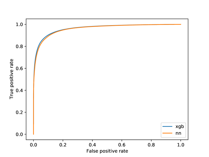
Figure 2: ROC curve of the trained NN (red) and GBDT (blue), for the event sample with $\not{E}_{T}\geq 10$ GeV.

In Fig. 2 we show the ROC curves of the trained NN and GBDT. In the control set with $\not{E}_{T}\geq 10$ GeV ($\not{E}_{T}\geq 100$ GeV), the overall AUC score is $0.9638$ ($0.9831$) for the GBDT, and $0.9605$ ($0.9819$) for the NN. Therefore, in our case, the GBDT very slightly outperforms the NN. The difference is hardly significant. Also, training a NN is considered to be more difficult, hence the NN performance could perhaps be further improved. However, since our scores are already rather close to the theoretical maximum of $1$, we instead proceed to extract sensitivity limits from these ML classifiers.

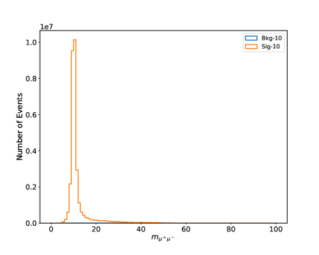
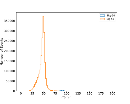
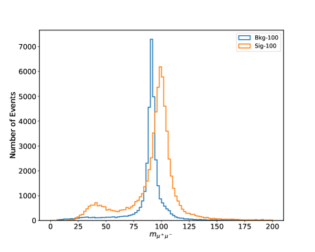
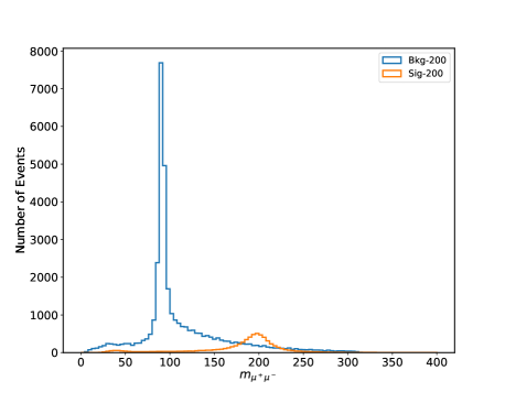
Figure 3: The distribution of $m^{(Z^{\prime})}_{\mu^{+}\mu^{-}}$, i.e. the di–muon invariant mass closer to $m_{Z^{\prime}}$. Here we use rescaled event numbers for a fixed luminosity, assuming $g_{\mu\tau}=1$. The top left, top right, bottom left and bottom right frames are for $m_{Z^{\prime}}=10$ GeV, $50$ GeV, $100$ GeV, and $200$ GeV, respectively.

For comparison, we also use dedicated simple cuts on the $3\mu$ events. We first remove events where a di–muon pair might have resulted from the decay of a (nearly) on–shell $Z$ boson, i.e. we require

$$|m_{\mu^{+}\mu^{-}}^{(1)}-91.19\ {\rm GeV}|\geq 8\ {\rm GeV}\,.$$ (6)

We then perform a simple (and idealized) “bump hunt”: we consider all events with

$$0.9\,m_{Z^{\prime}}\leq m_{\mu^{+}\mu^{-}}^{(Z^{\prime})}\leq 1.1\,m_{Z^{\prime}}$$ (7)

as signal, where $m_{\mu^{+}\mu^{-}}^{(Z^{\prime})}$ means the mass of the muon pair that is nearest to $m_{Z^{\prime}}$, the remaining events are considered background. Fig. 3 shows that for small $Z^{\prime}$ mass the second cut should capture nearly all signal events that pass the pre–selection cuts. For larger $m_{Z^{\prime}}$ there are also some signal events with $m_{\mu^{+}\mu^{-}}^{(Z^{\prime})}\sim 30$ to $50$ GeV; in these events at least one of the muons comes from the decay of a $\tau$ lepton. The lower frames of Fig. 3 show that the cut (6) should remove most of the background; in fact, from this figure the efficiency of this cut could be under–estimated, since it is applied to $m_{\mu^{+}\mu^{-}}^{(1)}$, which can be even closer to the $Z$ mass than the quantity $m_{\mu^{+}\mu^{-}}^{(Z^{\prime})}$ that is shown here. We also see that for unit coupling, the LHC signal is huge for $m_{Z^{\prime}}<m_{W}$, i.e. we expect a sensitivity limit well below $1$ for small $Z^{\prime}$ masses; however, the number of signal events evidently diminishes very quickly when the $Z^{\prime}$ mass is increased.

The cut (7) obviously depends on the $Z^{\prime}$ mass, which we assume to be known. In real life a hypothesis for this mass would have to be extracted from the data first, which is nontrivial for small signals; hence this search is idealized. We will see that nevertheless our ML classifiers, without prior knowledge of the $Z^{\prime}$ mass, outperform this idealized bump hunt.

4 Application to LHC Phenomenology

In this section we apply the classifiers described in the previous section. Either classifier allows to extract a sensitivity limit on the new coupling $g_{\mu\tau}$ as a function of $m_{Z^{\prime}}$. The GBDT in addition tells us which features are most useful for discriminating between signal and background. We will show how this information helps us to understand physical properties of the events; moreover, it allows to construct much simpler NN or GBDT classifiers, with far fewer input variables, that perform nearly as well as the original classifiers, which used $54$ input variables.

We already saw that both classifiers can quite efficiently discriminate between signal and background events. As a further check, following Ref. [17] we compare the normalized distributions of truth–level signal and background events with the distribution of events with $\hat{y}\geq\hat{y}_{\rm th}$, where the threshold $\hat{y}_{\rm th}$ is set such that $90\%$ of all events in the entire sample of simulated events that satisfy $\hat{y}\geq\hat{y}_{\rm th}$ are signal events; if the classifier works well, the latter distribution should therefore resemble that of truth–level signal events. We do this for several kinematic distribution, including both low–level and high–level features we used as input of our classifiers (see Table 1).

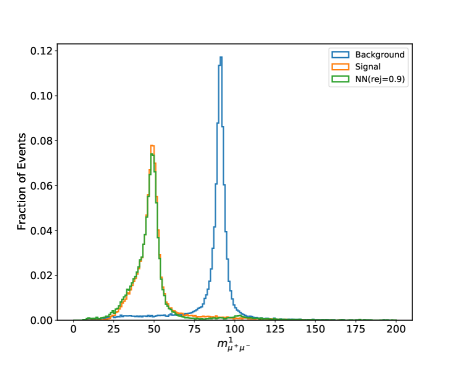
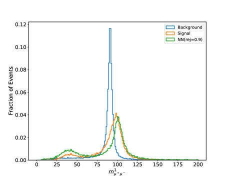
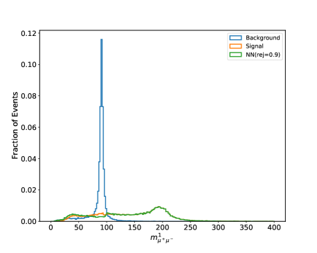
Figure 4: Normalized $m^{(1)}_{\mu^{+}\mu^{-}}$ distributions of $3\mu$ events, for $m_{Z^{\prime}}=10$ GeV (top left), $50$ GeV (top right), $100$ GeV (bottom left) and $200$ GeV (bottom right). The blue and orange histograms show the distributions for truth–level background and signal events, respectively, whereas the green histograms are for all events with NN output $\hat{y}\geq\hat{y}_{\rm th}$, where $\hat{y}_{\rm th}$ has been set such that $90\%$ of these events are signal events. The pre–selection cut $\not{E}_{T}\geq 10$ GeV has been used.

As example, we show the $m^{(1)}_{\mu^{+}\mu^{-}}$ distribution in Fig. 4, i.e. the distribution of the opposite–sign di–muon invariant mass whose invariant mass is closer to $m_{Z}$. Note that we only show events from the control samples here, which have not been used for training the NN. Not surprisingly, the background (shown in blue) peaks strongly at $m^{(1)}_{\mu^{+}\mu^{-}}=m_{Z}$ [hence the simple cut (6) used in our simple bump hunt will remove most of the background]. The distribution of signal events (shown in orange) depends strongly on the $Z^{\prime}$ mass. In particular, if $m_{Z^{\prime}}$ is not too far from $m_{Z}$ (top right and bottom left panels) there is a pronounced peak at $m^{(1)}_{\mu^{+}\mu^{-}}=m_{Z^{\prime}}$. For $m^{(1)}_{\mu^{+}\mu^{-}}\geq 100$ GeV there is also a second, broader and shallower, peak a $m^{(1)}_{\mu^{+}\mu^{-}}\simeq 35$ GeV, again due to $\tau\rightarrow\mu\nu_{\mu}\nu_{\tau}$ decays.

Most importantly, the distribution of events that are tagged as signal–like by the NN (green histogram) in most cases indeed resembles very closely that of truth–level signal events. The one exception occurs for $m_{Z^{\prime}}=100$ GeV (bottom left panel), where many background events from $\mu\nu_{\mu}Z$ production have very similar kinematics to our signal events. In Appendix B we also present distributions in $m^{(2)}_{\mu^{+}\mu^{-}},\ m_{T2}^{(1)},\ m_{T2}^{(2)},\ m_{T},\ p_{T}$ and $\not{E}_{T}$, where $m_{T}$ and $p_{T}$ refer to the muon with the largest transverse momentum. The green and orange histograms are again very similar, except for the case $m_{Z^{\prime}}=100$ GeV.

4.1 $3\mu$–Signal at the LHC without Dark Matter

In this subsection we derive the sensitivity limit on the coupling $g_{\mu\tau}$ from an analysis of simulated $3\mu$ events. We assume that the $Z^{\prime}$ cannot decay into Dark Matter particles, i.e. $m_{\rm DM}>m_{Z^{\prime}}/2$. In the region of $Z^{\prime}$ masses we are interested in, we then have ${\rm B}(Z^{\prime}\rightarrow\mu^{+}\mu^{-})={\rm B}(Z^{\prime}\rightarrow\tau^{+}\tau^{-})={\rm B}(Z^{\prime}\rightarrow\nu\bar{\nu})=1/3$. The sensitivity limit on $g_{\mu\tau}$ can therefore to very good approximation be interpreted as limit on $g_{\mu\tau}\sqrt{{\rm B}(Z^{\prime}\rightarrow\mu^{+}\mu^{-})/3}$.

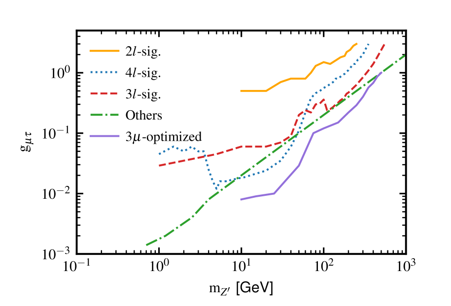
Figure 5: The best sensitivity for the $3\mu$ signal as function of $m_{Z^{\prime}}$. For $m_{Z^{\prime}}<100$ GeV the best results are from the pre–selection $\not{E}_{T}>10$ GeV, while for $m_{Z^{\prime}}>100$ GeV the best results are from the pre–selection $\not{E}_{T}>100$ GeV. Moreover, we add simulated data with $m_{Z^{\prime}}=15$, $25$, $75$, $150$, $250$, $350$, and $450$ GeV in order to check that our classifier is efficient for values of $m_{Z^{\prime}}$ on which it has not been trained.

The new sensitivity limit derived with the help of the NN is shown by the solid purple line in Fig. 5; this figure also shows the pre–LHC constraints (green dot–dashed) as well as bounds from published LHC searches with two (solid yellow), three (dashed red) and four (dotted blue) muons, all taken from our previous work [7]. In addition to the seven values of $m_{Z^{\prime}}$ we used for training of the NN, we generated data with $m_{Z^{\prime}}=15$, $25$, $75$, $150$, $250$, $350$, and $450$ GeV; evidently the NN also works for $Z^{\prime}$ masses on which it was not trained.

We see that use of the NN has the potential to improve the bound on $g_{\mu\tau}$ from previous LHC searches by a factor between two and four; it would then supersede the bound from non–LHC experiments for $10\ {\rm GeV}\leq m_{Z^{\prime}}\leq 500$ GeV. Recall also that this sensitivity limit assumes just $36\ {\rm fb}^{-1}$ of data; using the full run 2 statistics would improve the sensitivity by almost another factor of two. In principle LHC searches should also be sensitive to $Z^{\prime}$ masses below $10$ GeV; however, there Belle–2 will probably have better sensitivity. Of course, the sensitivity degrades with increasing $m_{Z^{\prime}}$, since the signal cross section for fixed coupling falls quickly when the $Z^{\prime}$ mass is increased, as we saw in Fig. 3. Nevertheless our results indicate that with full run 2 statistics, the LHC sensitivity could exceed the bound from pre–LHC experiments (from neutrino “trident” events observed by the CCFR collaboration [10], for $m_{Z^{\prime}}\geq 10$ GeV) for $Z^{\prime}$ masses up to $1$ TeV. The CCFR limit already means that the 1–loop $Z^{\prime}$ exchange contribution by itself cannot explain the discrepancy [3] in $g_{\mu}-2$; for couplings below our predicted sensitivity limit $Z^{\prime}$ contributions to $g_{\mu}-2$ would be essentially negligible.

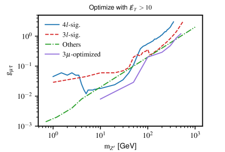
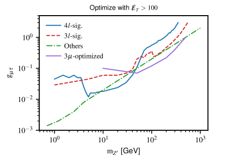
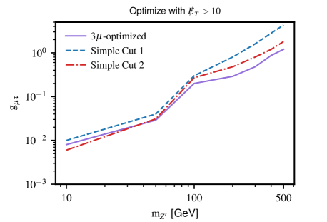
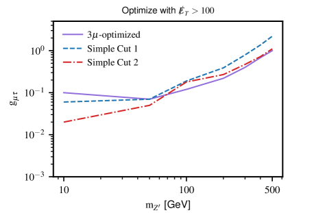
Figure 6: Impact of the pre–selection cut on missing $E_{T}$, with $\not{E}_{T}>10$ GeV (left) and $\not{E}_{T}>100$ GeV (right) respectively. The upper figures show the results from our previous publication (red, blue, green) [7] and ML classifiers (purple). In the lower figures, the optimized result through ML based classifier is compared to the results by successively applying the two simple cuts (6) (dashed blue) and (6) + (7) (dot–dashed red) in addition to the pre–selection cuts. The simple cuts are $m_{Z^{\prime}}$ dependent, while other curves are universal classifiers, which work for all $m_{Z^{\prime}}$.

The impact of the pre–selection cut on the missing $E_{T}$ on the performance of the NN is illustrated in Figs. 6. Requiring $\not{E}_{T}>100$ GeV removes many signal events with $m_{Z^{\prime}}<100$ GeV. Note that for $m_{Z^{\prime}}<80$ GeV the signal may originate from the decay of on–shell $W$ bosons; these events will typically have $\not{E}_{T}\>\raisebox{-2.15277pt}{$\stackrel{{\scriptstyle\textstyle<}}{{\sim}}$}\>m_{W}/2$. This cut therefore considerably degrades the performance for small $Z^{\prime}$ masses. On the other hand, removing most events with small $m_{Z^{\prime}}$ from the training sample improves the performance of the NN for $m_{Z^{\prime}}\geq$ 100 GeV. In this case signal events require far off–shell $W$ bosons, and one expects $\not{E}_{T}$ to be typically of order $m_{Z^{\prime}}$. The final sensitivity limit shown in Fig. 5 therefore comes from the larger event sample, with pre–selection cut $\not{E}_{T}\geq 10$ GeV, if $m_{Z^{\prime}}<100$ GeV, whereas for $m_{Z^{\prime}}\geq$ 100 GeV the stronger pre–selection cut $\not{E}_{T}\geq 100$ GeV yields better results.

We also tried training our ML classifiers without any $\not{E}_{T}$ cut. Even though the weaker cut $\not{E}_{T}\geq 10$ GeV only reduces the size of the sample by $\sim 5\%$, we found that removing this cut degrades the performance of the classifiers significantly. This illustrates the nonlinearity inherent to these ML methods.

The lower frames of Fig. 6 also show the sensitivity limit obtained from successively applying the simple cuts (6) and (7), using the same statistical method as for the NN classifier. Simply removing the background from on–shell $Z$ production via the cut (6) (dashed blue curves) already offers sizable sensitivity in our simulation. Recall, however, that we did not include backgrounds from heavy quarks; controlling them would certainly require additional cuts. The idealized bump hunt via the cut (7) further improves the sensitivity, but for $m_{Z^{\prime}}\geq 50$ GeV the NN with appropriate pre–selection cut still performs better. Recall also that we assumed $m_{Z^{\prime}}$ to be known when applying the cut (7); we did not impose a statistical price due to a look elsewhere effect, for example.

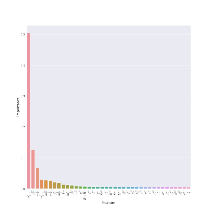
Figure 7: Feature importance as derived from the GBDT trained on the $3\mu$ sample with pre–selection cut $\not{E}_{T}>10$; the features are described in table 1. Here the indices $0,\,1$ and $2$ on $\mu$ stand for the muon with the highest, second highest, and lowest $p_{T}$, respectively. The feature importance is defined in XGBoost as the number of times a feature is used to split the data across all trees, normalized such that the sum over all features gives $1$.

The results shown in Figs. 5 and 6 have been obtained with the NN. The performance of the GBDT is very similar. Moreover, the latter allows to identify the most important features. As shown in figure 7, the top nine features that help to distinguish signal and background are $m_{\mu^{+}\mu^{-}}^{(1)}$, $p_{T}^{\mu 0}$, $m_{T2}^{(2)}$, $m_{\mu^{+}\mu^{-}}^{(2)}$, $m_{T}^{\mu 0}$, $m_{T2}^{(1)}$, $p_{T}^{\mu 1}$, $m_{T}^{\mu 1}$, and $\not{E}_{T}$. More than half of the $54$ original features have negligible importance. The large importance of the di–muon invariant mass closer to $m_{Z}$ indicates that the GBDT has “discovered” our simple cut (6), or something similar to it. This is also true for the GBDT trained on the reduced sample with $\not{E}_{T}\geq 100$ GeV; here the top nine features are $m_{\mu^{+}\mu^{-}}^{(1)}$, $m_{T2}^{(2)}$, $m_{T2}^{(1)}$, $p_{T}^{\mu 1}$, $m_{\mu^{+}\mu^{-}}^{(2)}$, $m_{T}^{\mu 1}$, $p_{T}^{\mu 0}$, $m_{T}^{\mu 2}$, and $m_{T}^{\mu 0}$.

Evidently most of the top features are high–level ones. In that sense the GBDT resembles typical cut–based LHC analyses, which often also crucially rely on some high–level features. Note that jet variables do not appear explicitly in either of these lists, although they are needed in the computation of the missing transverse momentum, and hence of all high–level features that depend on it (e.g. transverse masses). In our case jets are only emitted as radiation off the initial state, in both signal and background; it is therefore not surprising that the properties of the jets are similar in both kinds of events. Finally, at first sight it might seem somewhat surprising that the missing $E_{T}$ does not appear higher in the list of important features; after all, we saw above that the pre–selection cut on this quantity does affect the performance of the classifiers. Note, however, that “outliers” with very small $\not{E}_{T}$ appear in both signal and background, and the effect of the stronger cut $\not{E}_{T}\geq 100$ GeV was mostly to remove signal events with small $m_{Z^{\prime}}$. In contrast, the feature importance only shows how helpful a given feature is for distinguishing between signal and background.

In the next step we train simplified ML classifiers, which only include the top nine, six or even only top three features from these lists. This greatly reduces the computational effort. For example, in case of the NN the number of connections between “neurons”, and hence the number of weights that need to be determined during the training, scales quadratically with the number of features that serve as input into the NN.

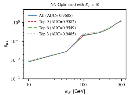
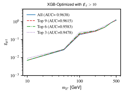
Figure 8: Sensitivity limits on $g_{\mu\tau}$ derived from an NN (left) and GBDT (right) that use all $54$ features (solid, blue), compared to the limits derived from simplified classifiers trained using only the top nine (dashed, red), top six (dot–dashed, green) or top three (dotted, purple) features.

The results for the event sample with $\not{E}_{T}\geq 10$ GeV are shown in Fig. 8. We see that the top six features are entirely sufficient to reproduce the performance of the original classifiers. Even just using the three most important features leads to only a small reduction in the sensitivity. Recall that we did not include backgrounds from the muonic decays of heavy quarks. Removing these backgrounds would certainly complicate the task of the ML classifiers. Nevertheless these results show that carefully selecting the input variables for the NN classifiers can greatly reduce the numerical effort, without significant degradation of the performance.

We also tried training our ML classifiers on the $45$ least important features, i.e. we remove the nine most important features from the list of input variables. The resulting NN still performs practically as good as the original one, i.e. it appears to be able to reconstruct the missing high–level features from the low–level ones that are still among the input variables. The performance of the GBDT does degrade a little bit, the sensitivity limit on $g_{\mu\tau}$ becoming typically $10$ to $20\%$ worse. In that sense the NN is somewhat more robust.

4.2 $2\mu$–Signal in LHC with DM Phenomenology

So far we have assumed that $Z^{\prime}\rightarrow\phi_{\rm DM}\bar{\phi}_{\rm DM}$ decays do not occur, either because they are kinematically forbidden or because $q_{\rm DM}=0$. As noted at the beginning of the previous Subsection, allowing such decays will reduce the number of $3\mu$ signal events somewhat, since they mostly originate from $Z^{\prime}\mu\nu_{\mu}$ production, with subdominant contributions from $Z^{\prime}\tau\nu_{\tau}$ production. In these production channels invisible $Z^{\prime}$ decay leads to a single lepton in the final state. This has a huge background from charged–current Drell-Yan production.

We can hope for a signal from invisible $Z^{\prime}$ decays therefore only from $\ell^{+}\ell^{-}Z^{\prime}$ production ($\ell=\mu,\tau$); the signal then contains a $\mu^{+}\mu^{-}$ pair and missing $E_{T}$. We saw in ref.[7] that this could have been detected in published di–muon searches only for parameters that are already excluded by published searches for $3\mu$ final states, unless the $L_{\mu}-L_{\tau}$ charge $q_{\rm DM}$ is very large, which does not look very plausible.

These conclusions were drawn from published searches that were not optimized for our model. Since the $2\mu$ signal suffers much larger background than the $3\mu$ signal, we expect the sensitivity to $g_{\mu\tau}$ in the former to still be worse than in the latter when dedicated ML classifiers are trained for both signals. However, a predicted sensitivity limit is not an experimental bound; after all, a dedicated $3\mu$ search might find a positive signal. Moreover, the strength of this signal would only allow to determine the product of the squared coupling and the muonic branching ratio of the $Z^{\prime}$, as already noted. Clearly we need a second, independent signal in order to determine these quantities separately, which in turn would allow us to learn something about Dark Matter in this model. To this end it is sufficient that the optimized sensitivity in the $2\mu$ channels is better than the existing bounds; it need not be comparable to the optimized sensitivity in the $3\mu$ channel.

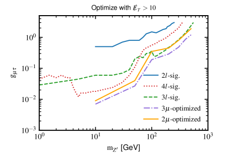
Figure 9: The solid light brown lines show the sensitivity limit predicted by the NN trained on $2\mu$ events, with pre–selection $\not{E}_{T}>10$ GeV (left) and $\not{E}_{T}>100$ GeV (right), respectively. The purple dot–dashed lines reiterate the sensitivity limit in the $3\mu$ channel derived in the previous subsection. The upper bounds on $g_{\mu\tau}$ extracted in [7] from published searches in the $2\mu,\ 3\mu$ and $4\mu$ channels are shown by the solid blue, dashed green and dotted red curves, respectively.

The sensitivity limit predicted by our NN trained on $2\mu$ events is shown in Fig. 9. The sensitivity is indeed weaker than that from the NN selected $3\mu$ signal, but they are comparable. In fact, the sensitivity limits from NNs trained on $2\mu$ and $3\mu$ events are much closer to each other than the existing bounds from published searches in the $2\mu$ and $3\mu$ channels [7]. For $m_{Z^{\prime}}<100$ GeV the best sensitivity again results from the pre–selection $\not{E}_{T}>10$ GeV, while for $m_{Z^{\prime}}>100$ GeV the best sensitivity is from the pre–selection $\not{E}_{T}>100$ GeV. Note that the sensitivity limit in the $2\mu$ channel predicted by the trained NN is below the best upper bound on $g_{\mu\tau}$ from published searches, including those in the $3\mu$ and $4\mu$ channels. This indicates that a dedicated search in the $2\mu$ channel might yet find a signal.

The GBDT again allows to extract the most important features. For both pre–selection cuts we find that the $p_{T}$ of the hardest muon and the di–muon invariant mass appear high in the list of most important features. As for the $3\mu$ signal most features we used are not very important. For both pre–selections, the five most important features account for more than $70\%$ of all branching decisions. Also in this case one could therefore (in hindsight) construct NNs and GBDTs with far few input variables, without significant loss of performance.

In Fig. 9 we have again assumed that $Z^{\prime}\rightarrow\phi_{\rm DM}\bar{\phi}_{\rm DM}$ decays are not possible. If these decays are allowed and $q_{\rm DM}$ is large enough, the sensitivity in the $2\mu$ channel might even be higher than that in the $3\mu$ channel. We saw above that the number of $3\mu$ signal events is reduced when the invisible branching ratio of the $Z^{\prime}$ boson is increased. The $2\mu$ signal gets contributions from several diagrams: $\nu_{\ell}\bar{\nu}_{\ell}Z^{\prime}$ and $\ell\nu_{\ell}Z^{\prime}$ production followed by visible $Z^{\prime}$ decays, and $\ell^{+}\ell^{-}Z^{\prime}$ production followed by invisible $Z^{\prime}$ decays, with $\ell=\mu,\,\tau$. The former contributions decrease with increasing invisible width of the $Z^{\prime}$, but the latter increases. Hence the total $2\mu$ signal is less sensitive to the invisible width of the $Z^{\prime}$ than the $3\mu$ signal. In order to probe this quantitatively, we assume $\phi_{\rm DM}$ to be light, $m^{2}_{\rm DM}\ll m^{2}_{Z^{\prime}}$, and consider scenarios with $q_{\rm DM}=1$ and $2$. We use the classifier trained without $Z^{\prime}$ decays into Dark Matter particles, without retraining.

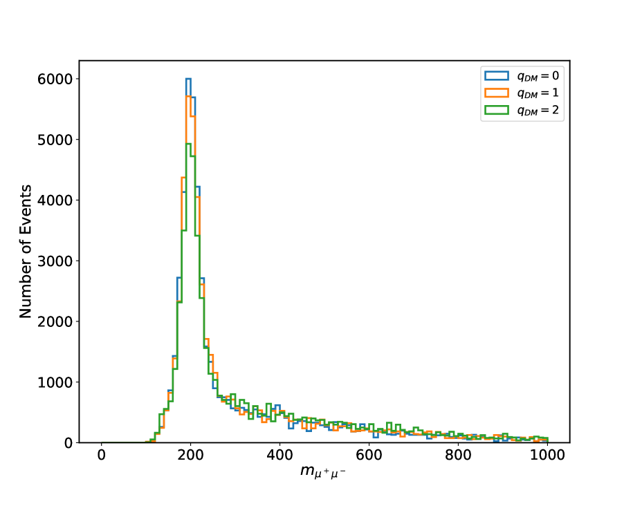
Figure 10: Distribution of $m_{\mu^{+}\mu^{-}}$ for the $2\mu$–signal with $m_{Z^{\prime}}=200$ GeV and the DM $L_{\mu}-L_{\tau}$ charge $q_{\rm DM}=0$ (blue), $1$ (orange) and $2$ (green). The $y$ axis is scaled to the total cross section. Only $Z^{\prime}$ production events tagged as signal by the NN are shown.

The above discussion shows that the invisible branching ratio of the $Z^{\prime}$ boson can also be obtained not only from the ratio of $3\mu$ and $2\mu$ events, but also from the $\mu^{+}\mu^{-}$ invariant mass distribution in $2\mu$ events. Increasing the invisible branching ratio reduces the branching ratio for $Z^{\prime}\rightarrow\mu^{+}\mu^{-}$ events, and hence the number of signal events with $m_{\mu^{+}\mu^{-}}\simeq m_{Z^{\prime}}$. On the other hand, increasing the invisible branching ratio increases the contribution from $\ell^{+}\ell^{-}Z^{\prime}$ production followed by invisible $Z^{\prime}$ decay which mostly produces $\mu^{+}\mu^{-}$ pairs with invariant mass distinct from $m_{Z^{\prime}}$. It should be noted, however, that the “off–peak” part of the signal also receives significant contributions from $\mu\nu_{\mu}Z^{\prime}$ production where the $Z^{\prime}$ produces exactly one muon which passes the pre–selection cuts; this can be due to $Z^{\prime}\rightarrow\tau^{+}\tau^{-}$ decays with only one $\tau$ lepton producing a detectable muon, or due to $Z^{\prime}\rightarrow\mu^{+}\mu^{-}$ decays with one muon having too large rapidity or too small $p_{T}$. This contribution to the off–peak signal will decrease when $q_{\rm DM}$ is increased. The $q_{\rm DM}$ dependence of the off–peak part of the signal can therefore only be predicted from Monte Carlo studies.

This is shown in Fig. 10. Increasing the DM charge from $0$ (blue) to $2$ (green) clearly reduces the height of the peak at $m_{\mu^{+}\mu^{-}}=m_{Z^{\prime}}$, but has much less effect on the plateau of signal events away from the peak.

DM Charge	${\rm Br}(Z^{\prime}\rightarrow\mu^{+}\mu^{-})$	${\rm Br}(Z^{\prime}\rightarrow{\rm invisible})$	$N_{\rm peak}/N_{\rm off\ peak}$
0	$0.333$	$0.333$	$0.620$ $(0.233)$
1	$0.308$	$0.385$	$0.595$ $(0.230)$
2	$0.25$	$0.5$	$0.476$ $(0.209)$

Table 2: The second and third column shows the muonic and invisible branching ratios of the $Z^{\prime}$ boson, respectively, for different values of the $L_{\mu}-L_{\tau}$ charge $q_{\rm DM}$ of the Dark Matter particle. The last column gives the ratio of the number of events in the peak, defined by $180\ {\rm GeV}\leq m_{\mu^{+}\mu^{-}}\leq 220$ GeV, divided by the number of events off the peak, defined by $m_{\mu^{+}\mu^{-}}<180$ GeV or $m_{\mu^{+}\mu^{-}}>220$ GeV, for $m_{Z^{\prime}}=200$ GeV; the first number only includes true signal events, whereas the number in parentheses also includes the background and assumes $g_{\mu\tau}=0.4$. Only $2\mu$ events selected by our NN classifier as signal–like, with pre–selection $\not{E}_{T}\geq 100$ GeV, have been included.

In order to investigate this more quantitatively, we propose to use the ratio of on–peak and off–peak events as variable that is sensitive to possible $Z^{\prime}$ decays into Dark Matter particles. For $m^{2}_{\rm DM}\ll m^{2}_{Z^{\prime}}$ and $m^{2}_{Z^{\prime}}\gg m_{\ell}^{2}$, eqs.(2) and (3) give:

$${\rm Br}(Z^{\prime}\rightarrow\mu^{+}\mu^{-}) \simeq \frac{4}{12+q^{2}_{\rm DM}}\,;$$

$${\rm Br}(Z^{\prime}\rightarrow{\rm invisible}) \simeq \frac{4+q^{2}_{\rm DM}}{12+q^{2}_{\rm DM}}\,.$$ (8)

The corresponding values are given in the second and third column of Table 2.

This table shows that the ratio of signal events near and away from the $Z^{\prime}$ peak indeed depends quite sensitively on the invisible width of the $Z^{\prime}$, and hence on $q_{\rm DM}$. Here we have used a higher threshold of the NN classifier for the definition of “signal” events than in Fig. 9, in order to enhance $S/B$ which makes the total event distribution more signal–like. In the absence of background the ratio of the number of on–peak and off–peak events is independent of the coupling $g_{\mu\tau}$, as long as the width $\Gamma_{Z^{\prime}}<0.1m_{Z^{\prime}}$. When including the background we used the largest still allowed coupling, $g_{\mu\tau}=0.4$ for the chosen $Z^{\prime}$ mass of $200$ GeV. This results in similar numbers of signal and background events on the peak, but the background still dominates off–peak. As a result, one would need an integrated luminosity of at least $2$ ab^-1 in order to see a significant difference between $q_{\rm DM}=0$ and $q_{\rm DM}=2$, even for $g_{\mu\tau}=0.4$.

5 Summary and Conclusions

In this study, we used ML based classifiers to optimize the search for signals for the production of the new gauge boson $Z^{\prime}$ predicted by the extension of the SM by the gauge group $U(1)_{L_{\mu}-L_{\tau}}$ at the LHC. Our model also contains a Dark Matter particle, but we ignore possible contributions from the additional Higgs boson as well as the heavy neutrinos that are also predicted by this model. We had seen in a previous analysis that published ATLAS and CMS searches for multi–lepton final states lead to an upper bound on the coupling of the new gauge boson that in most cases is worse than that from pre–LHC experiments.

We constructed both neural network (NN) and gradient-boosted decision tree (GBDT) classifiers. Both lead to much improved sensitivity limits for a given luminosity, compared to those we derived earlier from published searches; hence the ML classifiers would allow to probe regions of parameter space that are still allowed. In particular, in the absence of a signal, for the considered range $m_{Z^{\prime}}\geq 10$ GeV contributions from $Z^{\prime}$ loops to the anomalous magnetic moment of the muon would be constrained to be considerably smaller than the present uncertainty on this quantity, in which case this contribution could safely be neglected; the existing constraints already imply that $Z^{\prime}$ loops by themselves cannot fully explain the discrepancy between theory and experiment. The ML classifiers also lead to somewhat better sensitivity than a simple “bump hunt”.

We initially used a very large number of input parameters, or features, for training our classifiers. The GBDT allows to extract the importance these features played in the construction of the final classifier. Using only the six most important features led to greatly simplified classifiers which nevertheless performed practically as well as the original ones. Moreover, most of the important features are high–level ones, similar to observables that have been used in traditional cut–based analyses. On the other hand, yet another NN trained on all except the most important features still performs as well as the original one, showing that the NN can “learn” the relevant high–level features by itself; however, a GBDT trained on this reduced set of features performs slightly worse than the original one.

We emphasize that our classifiers were trained on event samples containing signal events with many different values of the $Z^{\prime}$ mass; we found that they work nearly as well for $Z^{\prime}$ masses not covered in the training set. Nevertheless our optimization was not completely automatic. We needed a mild pre–selection cut on the missing $E_{T}$, $\not{E}_{T}\geq 10$ GeV, in order to remove “outliers” in both signal and background events. Moreover, for $m_{Z^{\prime}}>100$ GeV the sensitivity was improved if the much stronger pre–selection $\not{E}_{T}\geq 100$ GeV was used; this stronger cut greatly reduces the number of signal events with small $Z^{\prime}$ masses in the training sample. We found that the $3\mu$ channel offers better sensitivity, but the shape of the $\mu^{+}\mu^{-}$ invariant mass distribution in the $2\mu$ channel might allow to determine the invisible branching ratio of the $Z^{\prime}$, which in turn could constrain the $L_{\mu}-L_{\tau}$ charge of the Dark Matter particle.

Our analysis is still not entirely realistic. For one thing, we only included backgrounds that have the same partonic final states as the signal; in particular, we did not include backgrounds from the production and semi–leptonic decays of heavy quarks, which however should be relatively easier to distinguish from the signal. Moreover, in the estimate of the final sensitivity we did not attempt to estimate systematic uncertainties on the background. We note, however, that most of the background can be estimated directly from data, by simply replacing muons by electrons in the final state. Finally, our detector model is based on that used in CheckMATE.

The methods we used should nevertheless be useful also for the analysis of experimental searches using real data, for these or other final states. In particular, using a GBDT trained on a large number of input variables in order to pin down the most important features, which in turn allows to construct a simplified NN, might allow to construct a largely automated “pipeline” for such searches.

ACKNOWLEDGEMENTS

We thank Ian Brock for the suggestion to use events with electrons for background estimates. This work was partially supported by the by the German ministry for scientific research (BMBF).

Appendix A ML Classifiers in a Nutshell

In this appendix we provide a brief tutorial on the construction and training of ML classifiers. We first make some remarks on supervised machine learning, before briefly describing GBDTs and NNs, respectively.

A.1 Supervised Machine Learning

A machine learning algorithm is an algorithm that is able to learn from (real or simulated) data [33]. One distinguishes between supervised and unsupervised learning, depending on whether each data is provided with a pre–defined label or not; in our case the labels are “signal” and “background”, i.e. we will focus on binary supervised classification algorithms in this appendix. Mathematically speaking, the algorithms or “models” are trying to learn a mapping $f(\boldsymbol{x}):\mathcal{X}\to\mathcal{Y}$, where the vector $\boldsymbol{x}_{i}\subset\mathcal{X}$ is the $i-$th data set, and $\mathcal{Y}\subseteq\{0,1\}$ is the output, where $Y=0\ (1)$ means that the event is classified as background (signal).

The learning process is terminated when the performance on an independent control sample reaches an optimum. The performance can be evaluated by a metric function, such as accuracy, which is simply the fraction of correctly identified events. Also, it is important to emphasize that the model must be tested on data not used for the training. This can be done in a simple way called "hold-out" validation. To that end we randomly split the generated events it into training and test sets. As indicated by its name, the training set is used to train the model, and the test set to test its performance. Usually, the model’s performance differs in these two data sets. If after training the performance is bad on the training set, it is called underfitting; this could mean that the classifier is not sufficiently sophisticated. In contrast, the model might be overfitted if it performs much worse on the test set compared than on the training set. Overfitting is one of the major topics in machine learning, it occurs when the model’s capacity is so large that it learns the local variance of training data. To avoid overfitting, some specialized techniques like regularization are applied to the model in order to limit its capacity; we refer to the literature [33] for further details.

In the following subsections, we will briefly introduce the two machine learning algorithms we used in this paper, XGBoost and neural network. We will cover the basic ideas behind these algorithms.

A.2 XGBoost

A.2.1 Decision Tree

Before we dive into the details of XGBoost, we first introduce its basic structure, the decision tree. A decision tree is a tree–like structure, consisting of a root node, multiple internal nodes, and leaf nodes. The prediction process for each event starts from the root node, checks its attribute and follows the conditional flow, which takes one to a lower node. This is repeated until one reaches one of the leaf nodes. Then, the score or label of this leaf node gives the final output of the decision tree for this event.

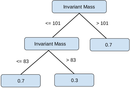
Figure 11: An example of a decision tree structure. It is built by the invariant mass of muon pairs. The numbers on the branches are in GeV, and those on the leaves show how signal–like the event is.

For example, let’s consider the process $pp\to 2\mu+\not{E}_{T}$, where $\not{E}_{T}$ means invisible particles, e.g. neutrinos or DM. Consider the simple decision tree shown in Fig. 11 acting on an event with invariant mass $m_{\mu^{+}\mu^{-}}=95$ GeV. According to Fig. 11, we first compare the value with the attribute in root node (the top one), if it is smaller than $101$, we go left, otherwise right. By repeating this process, we finally reach a leaf node (node without any splitting) with score $0.3$ on the bottom right. The score is higher for more signal–like events; a score of $0.3$ thus means that our simple decision tree predicts the event to likely be a background event.

It is obvious that a key aspect in the training of a decision tree is how to split a node. This includes how to choose an attribute among the list of features, here the invariant mass, and how to split according to the chosen attribute (the conditional flow). An algorithm named ID3 (Iterative Dichotomiser 3) is often used. It is based on information entropy,

$$\textbf{Ent}(\mathcal{D})=-\sum_{k=0}^{|\mathcal{Y}|-1}p_{k}~{}\log_{2}~{}p_{k}\,,$$ (A1)

where $\mathcal{D}=\{(\mathbf{x}_{i},y_{i})\}$ is the set of all events and their labels, and $p_{k}$ is the fraction of events labeled $k$. The information entropy represents the impurity of data, a smaller value means they are more likely being correctly classified. In our problem we have only two labels, hence Ent$(\mathcal{D})=-p_{0}\log_{2}p_{0}$. This vanishes for samples containing either only signal ($p_{0}=0$) or only background ($p_{0}=1$) events, and reaches a maximum of about $0.531$ for $p_{0}=1/{\rm e}\simeq 0.368$, not far from the intuitively most mixed case $p_{0}=1/2$.

For a given attribute $a$ and a possible splitting condition, we can split the original set $\mathcal{D}$ into two sets $\mathcal{D}_{L}$ and $\mathcal{D}_{R}$. The information gain from this splitting is then

$$\textbf{Gain}(\mathcal{D},a)=\textbf{Ent}(\mathcal{D})-\frac{|\mathcal{D}_{L}|}{|\mathcal{D}|}\textbf{Ent}(\mathcal{D}_{L})-\frac{|\mathcal{D}_{R}|}{|\mathcal{D}|}\textbf{Ent}(\mathcal{D}_{R})\,.$$ (A2)

Generally speaking, the information gain measures how much the purity improves if one makes this splitting. Hence, if we go through all possible attributes and splitting conditions, we can determine the current best split as the one which maximizes the information gain; this of course depends on the set of events to which this splitting is applied. By always choosing the best split, we finally obtain a decision tree.

A.2.2 Gradient Boosting Decision Tree

The ability of a single decision tree is usually limited, especially when the task is complicated. One way to improve its performance is by using an ensemble of many decision trees, and taking the sum as prediction[34]:

$$\hat{y}_{i}=\phi(\boldsymbol{x}_{i})=\frac{1}{V}\sum_{v=1}^{V}f_{v}(\boldsymbol{x}_{i})\,.$$ (A3)

Here $\hat{y}_{i}$ is the final output (“score”) of event $i$ and $V$ is the number of trees. We take the same process $pp\to 2\mu+\not{E}_{T}$ as an example. For an event with $m_{\mu^{+}\mu^{-}}=95$ GeV and $\not{E}_{T}=110$ GeV, we get the prediction of the decision trees in Fig. 12 through the “vote” of 2 trees:

$$\hat{y}=\frac{1}{2}(f_{1}(\boldsymbol{x})+f_{2}(\boldsymbol{x}))=\frac{1}{2}(0.3+0.6)=0.45$$ (A4)

Note that we take an average of these two scores so that the answer lies between $0$ and $1$ if each individual score lies between these values.

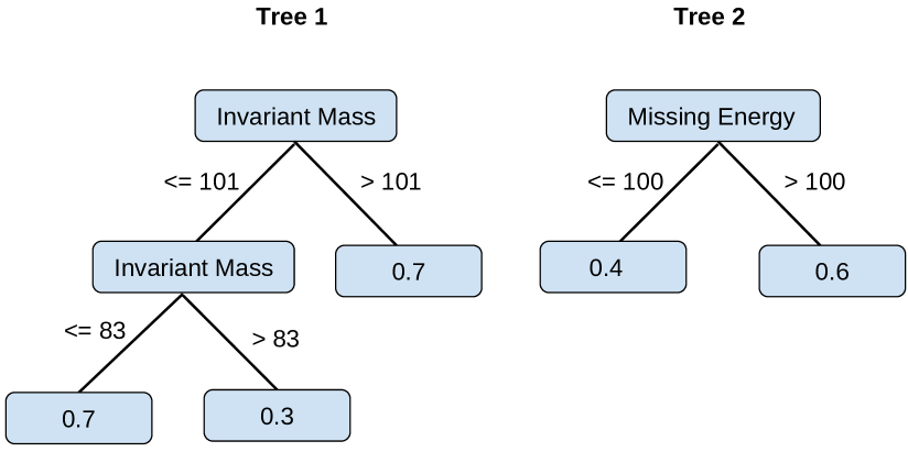
Figure 12: An ensemble of decision trees constructed with $m_{\mu^{+}\mu^{-}}$ and $\not{E}_{T}$.

However, a naive ensemble where one simply averages over all scores, is not good enough for some tasks. We instead use a more powerful algorithm named GBDT (Gradient Boosting Decision Tree) [35]. GBDT also generates an ensemble of decision trees. But there are two major differences: firstly, GBDT generates trees iteratively, which means that the $t-$th tree is dependent on the previous $t-1$ trees, this is the so called boosting algorithm; secondly, GBDT generalizes the process of finding the best split to minimize a predefined objective function.

In XGBoost, the objective function is written as[34]

$$\mathcal{L}(\phi)=\sum_{i}l(\hat{y}_{i},\,y_{i})+\sum_{v}\Omega(f_{v}),\quad\textrm{where}\quad\Omega(f)=\gamma T+\frac{1}{2}\lambda\|w\|^{2}\,.$$ (A5)

Here $\gamma$ and $\lambda$ are hyperparameters to be defined externally, $T$ is the number of leaves in the tree $f$ and $||w||$ is the sum of the scores of all leaves. Moreover, $l$ is a differentiable loss function that measures the difference between the output $\hat{y}_{i}$ and the true $y_{i}$. In the case of binary classification task, it can be the binary cross entropy loss,

$$l(\hat{y}_{i},\,y_{i})=-y_{i}~{}\log~{}\hat{y}_{i}-(1-y_{i})~{}\log~{}(1-\hat{y}_{i})\,.$$ (A6)

Finally, $\Omega$ in eq.(A5) is a regularization term which penalizes the complexity of the model, thereby limiting the number of leaves.

Next, we will discuss how to iteratively generate trees. Let $\hat{y}_{i}^{t-1}$ be the prediction of the previous $t-1$ trees. The $t-$th tree $f_{t}$ is then generated by minimizing the loss function of eq. (A5), i.e.

$$\mathcal{L}^{t}=\sum_{i}l(y_{i},\,\hat{y}_{i}^{(t-1)}+f_{t}(\boldsymbol{x}_{i}))+\Omega(f_{t})\,.$$ (A7)

After Taylor expanding up to second order and ignoring constant terms, we obtain a simplified objective function for the $t$–th iteration[34]:

$$\tilde{\mathcal{L}}^{t}=\sum_{i}[g_{i}f_{t}(\boldsymbol{x}_{i})+\frac{1}{2}h_{i}f_{t}^{2}(\boldsymbol{x}_{i})]\\ +\Omega(f_{t})\,.$$ (A8)

Here $g_{i}=\partial_{\hat{y}_{i}^{(t-1)}}l(y_{i},\,\hat{y}_{i}^{(t-1)})$ and $h_{i}=\partial_{\hat{y}_{i}^{(t-1)}}^{2}l(y_{i},\,\hat{y}_{i}^{(t-1)})$ are the gradients. The optimal objective value turns out to be [34]:

$$\tilde{\mathcal{L}}^{t\ast}=-\frac{1}{2}\sum_{j=1}^{T}\\ \frac{(\sum_{i\in I_{j}}g_{i})^{2}}{\sum_{i\in I_{j}}h_{i}+\lambda}+\gamma T\,.$$ (A9)

Here $I_{j}$ is the set of events that reach leaf $j$ according to the splitting rules of a given tree. Eq. (A9) is like the impurity score; we can use it to find the best split by maximizing the loss reduction:

$$\mathcal{L}_{\rm split}=\frac{1}{2}\left[\frac{(\sum_{i\in I_{L}}g_{i})^{2}}{\sum_{i\in I_{L}}h_{i}+\lambda}\\ +\frac{(\sum_{i\in I_{R}}g_{i})^{2}}{\sum_{i\in I_{R}}h_{i}+\lambda}\\ -\frac{(\sum_{i\in I}g_{i})^{2}}{\sum_{i\in I}h_{i}+\lambda}\right]-\gamma\,.$$ (A10)

This is similar to maximizing the information gain in the previous subsection. A similar consideration determines the optimal scores on the leaves of the tree. By repeating this process, we can obtain a sequence of decision trees.

Since we need to go through all possible splits, the time complexity to find a single best split is $\mathcal{O}(n\times m)$, where $n$ is the number of events and $m$ is the number of features. This is extremely time consuming, so XGBoost uses some approximate algorithms to speed it up. The details can be found in Ref. [34].

A.3 Neural Network

A simple example of a neural network is a feed–forward neural network, or multilayer perceptron (MLP). It is called feed–forward since the information flows from the input to some intermediate units, and finally to the outputs without any feedback connections. If we consider a sample with $m=3$ features $\boldsymbol{x}=(x_{1},x_{2},...,x_{m})$, then a 2–layer feed–forward neural network is shown in Fig. 13. Note that we use bold face $\boldsymbol{x}_{i}$ representing the $i-$th event in the data set, and $x_{a}$ for the $a-$th feature of an event.

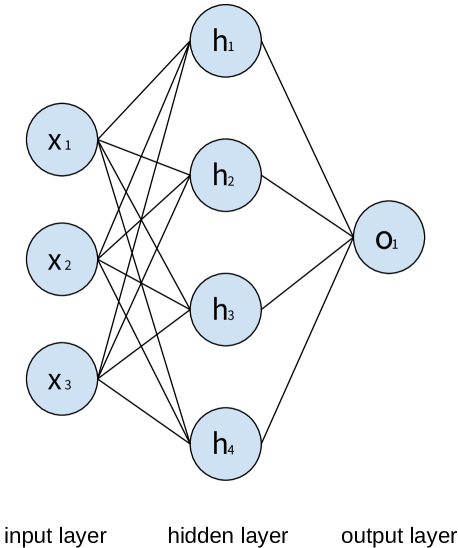
Figure 13: The structure of a 2–layer feed–forward neural network. Note that we usually do not count the input layer.

The $a-$th node in the input layer simply passes on the value of the $a-$th feature of a given event. For the subsequent layers, the input ${\cal I}$ into each node (“neuron”) is a linear combination of the outputs of all the units in the previous layer to which it is connected. For example,

$${\cal I}_{1}=W_{11}x_{1}+W_{12}x_{2}+W_{13}x_{3}+b_{1}\quad\Leftrightarrow\quad\boldsymbol{{\cal I}}=\boldsymbol{W}\boldsymbol{x}+\boldsymbol{b}\,.$$ (A11)

Here the weights $\boldsymbol{W}$ and biases $\boldsymbol{b}$ are learnable parameters of the NN. A purely linear NN is often not very good at solving complex tasks. The output ${\cal O}$ of a given neuron is therefore a non–linear function $\sigma$ of the input, so that the NN can learn non–linear mapping:

$$\boldsymbol{{\cal O}}=\sigma(\boldsymbol{W}\boldsymbol{x}+\boldsymbol{b})\,.$$ (A12)

$\sigma$ is also called the activation function. A commonly used activation function in hidden layers is ReLU (Rectified Linear Unit) function,

$$\textbf{ReLU}(x)=\textbf{max}(0,x)\,.$$ (A13)

The activation function of the neurons in the output layer depends on the specific task. In our case, which is a binary classification problem, we use the sigmoid function, since it maps any real number into $[0,\,1]$:

$$\textbf{Sigmoid}(x)=\frac{1}{1+e^{-x}}\,.$$ (A14)

In summary, the final score $\hat{y}$ of the neural network in Fig. 13 is

$$\boldsymbol{{\cal O}^{h}}=\textbf{ReLU}(\boldsymbol{W}^{h}\boldsymbol{x}+\boldsymbol{b}^{h})\quad\textrm{and}\quad\hat{y}=\textbf{Sigmoid}(\boldsymbol{W}^{o}\boldsymbol{{\cal O}^{h}}+\boldsymbol{b}^{o})\,,$$ (A15)

where we have introduced superscripts $h$ and $o$ to label the weights and biases of the hidden and output layers, respectively.

In order to determine the parameters $\boldsymbol{W}$ and $\boldsymbol{b}$ in a neural network, one minimizes an objective function similar to Eq. (A5),

$$\mathcal{L}=\sum_{i}l(\hat{y}_{i},\,y_{i})+\Omega$$ (A16)

where $\Omega$ is again a regularization term, and $l(\hat{y}_{i},y_{i})$ is the same loss function as in Eq. (A6). Due to the nonlinearity of a neural network, the objective function in general becomes nonconvex. It is common to use gradient descent to find the minimum, which is taking steps in the opposite direction of the gradient until reaching a local minimum. We initialize $\boldsymbol{W}$ and $\boldsymbol{b}$ to small random values. The simplest gradient–based rule for updating them can be written as

$$\boldsymbol{W}=\boldsymbol{W}-\eta\cdot\nabla_{\boldsymbol{W}}\mathcal{L}\quad\textrm{and}\quad\boldsymbol{b}=\boldsymbol{b}-\eta\cdot\nabla_{\boldsymbol{b}}\mathcal{L}\,,$$ (A17)

where $\eta$ is the learning rate. In practice we use more efficient algorithms to update the parameters. They are also based on gradients, but more efficient and more likely to jump out of local minima. These are called optimizers in deep learning, like Adam that we used in this paper.

There are some other techniques that we used in this paper, such as Dropout [36] to prevent overfitting and Batch Normalization [37] to speed up convergence, which we do not discuss in detail here.

Appendix B: Additional Figures

In this Appendix we collect some more figures. The first four figures give GBDT determined feature importances. The remaining figures give kinematical distributions for true signal events, true background events, and events classified as signal–like by the NN. Here we have set the threshold $\hat{y}_{\rm th}$ such that $90\%$ of all events with $\hat{y}\geq\hat{y}_{\rm th}$ are signal events, where “all events” refers to the entire sample of simulated events.

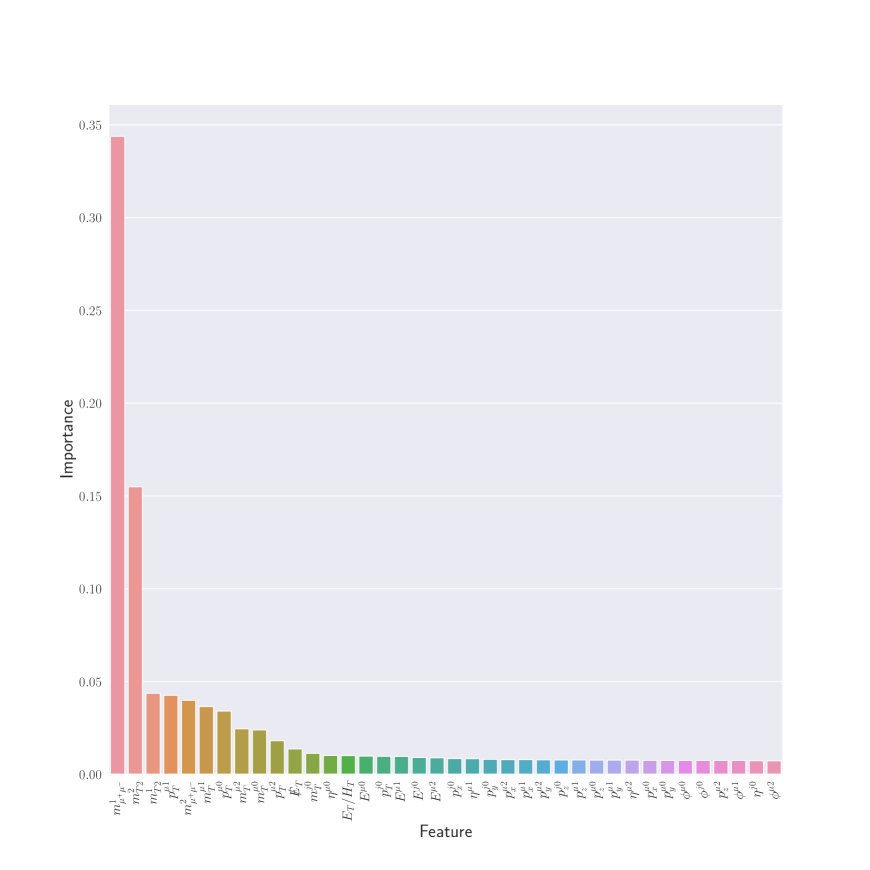
Figure 14: Feature importance for the $3\mu$ signal with pre–selection $\not{E}_{T}>100$ GeV from XGBoost. The features are listed in table 1. The most influential features are $m_{\mu^{+}\mu^{-}}^{(1)}$, $m_{T2}^{(2)}$, $m_{T2}^{(1)}$, $p_{T}^{\mu_{1}}$, $m_{\mu^{+}\mu^{-}}^{(2)}$, $m_{T}^{\mu_{1}}$, $p_{T}^{\mu_{0}}$, $m_{T}^{\mu_{2}}$, and $m_{T}^{\mu_{0}}$.

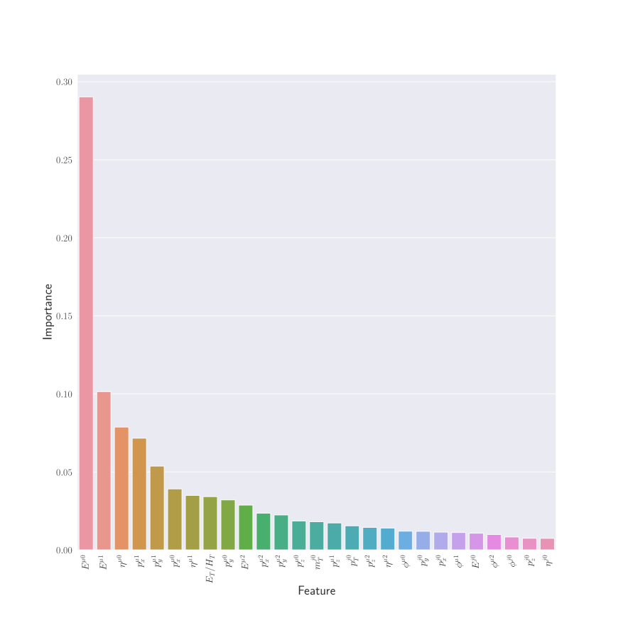
Figure 15: Feature importance for the $3\mu$ signal with pre–selection $\not{E}_{T}>10$ GeV. Here we trained a GBDT by excluding the top 9 features of the original GBDT. The most influential features are now $E^{\mu_{0}}$, $E^{\mu_{1}}$, $\eta^{\mu_{0}}$, $p_{x}^{\mu_{1}}$, $p_{y}^{\mu_{1}}$, $p_{x}^{\mu_{0}}$, $\eta^{\mu_{1}}$, $E_{T}/H_{T}$, and $p_{y}^{\mu_{0}}$.

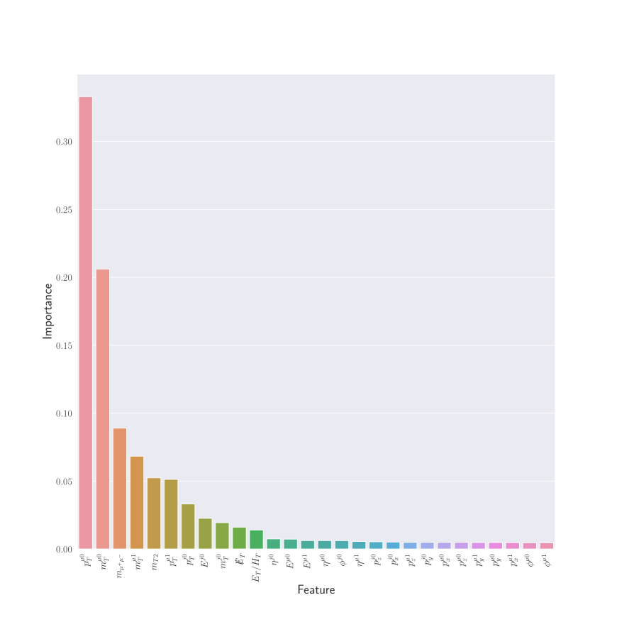
Figure 16: Feature importance for the $2\mu$ signal with pre–selection $\not{E}_{T}>10$ GeV from XGBoost. The features are listed in table 1. The most influential features are $p_{T}^{\mu_{0}}$, $m_{T}^{\mu_{0}}$, $m_{\mu^{+}\mu^{-}}$, $m^{\mu_{1}}_{T}$, $m_{T2}$, $p_{T}^{\mu_{1}}$, $p_{T}^{j_{0}}$, $E^{j_{0}}$, $m_{T}^{j_{0}}$, and $\not{E}_{T}$.

Figure 17: Feature importance for the $2\mu$ signal with pre–selection $\not{E}_{T}>100$ GeV from XGBoost. The features are listed in table 1. The most influential features are $m_{\mu^{+}\mu^{-}}$, $p_{T}^{\mu_{0}}$, $m_{T2}$, $p_{T}^{\mu_{1}}$, $m_{T}^{\mu_{0}}$, $p_{T}^{j_{0}}$, $m^{\mu_{1}}_{T}$, $E_{T}/H_{T}$, $\not{E}_{T}$ and $m_{T}^{j_{0}}$.

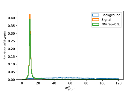
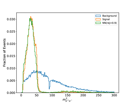
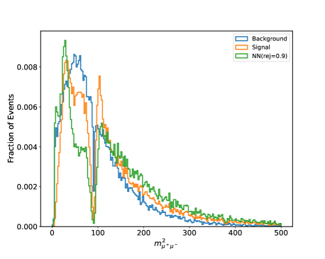
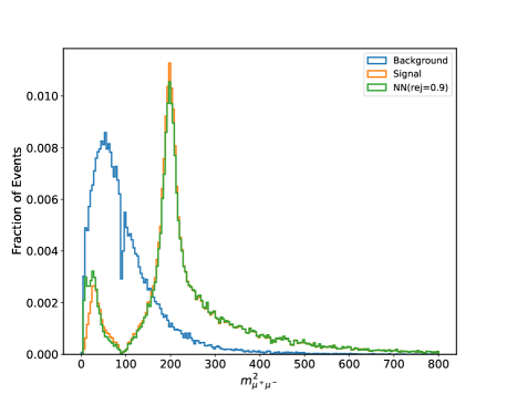
Figure 18: Di–muon invariant mass distribution of $3\mu$ events, where the $\mu^{+}\mu^{-}$ pair is chosen whose invariant mass is furthest away from $m_{Z}=91.19$ GeV. The top left, top right, bottom left and bottom right frames are for $m_{Z^{\prime}}=10,\,50,\,100$ and $200$ GeV, respectively. The blue and orange histograms show pure background and pure signal events, respectively, while the green histogram is for events that have been flagged as signal–like by the NN, with threshold such that $90\%$ of accepted events are true signal events.

Figure 19: As in Fig. 18, except that now the distribution in $m_{T2}^{(1)}$ is shown, i.e. the $m_{T2}$ variable of the $\mu^{+}\mu^{-}$ pair whose invariant mass is closest to $m_{Z}$.

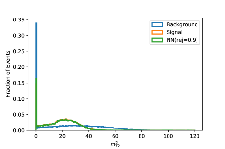
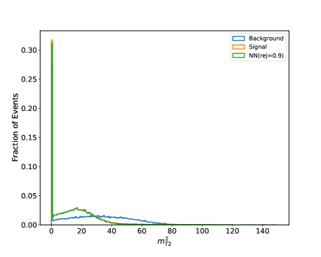
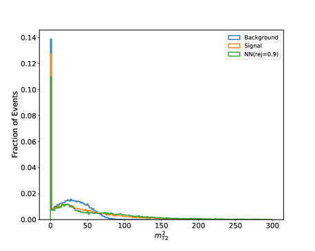
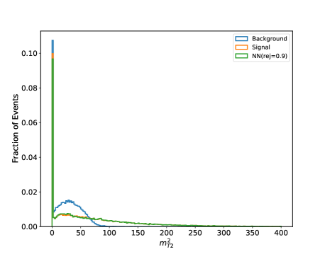
Figure 20: As in Fig. 18, except that now the distribution in $m_{T2}^{(2)}$ is shown, i.e. the $m_{T2}$ variable of the $\mu^{+}\mu^{-}$ pair whose invariant mass is furthest from $m_{Z}$.

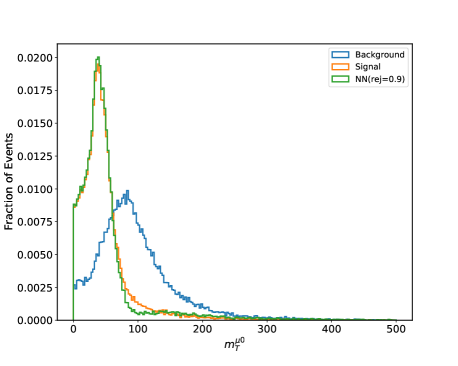
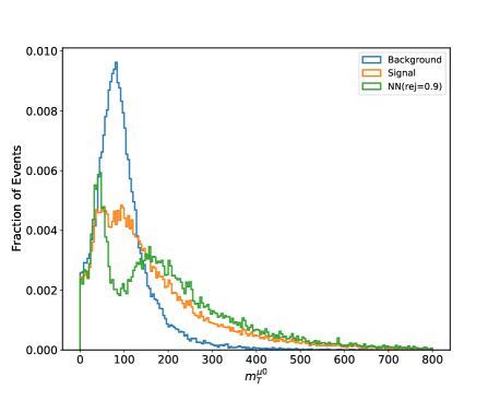
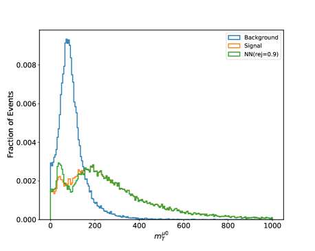
Figure 21: As in Fig. 18, except that now the distribution in $m_{T}^{(0)}$ is shown, i.e. the transverse mass of the muon with the largest $p_{T}$.

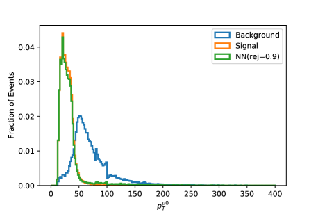
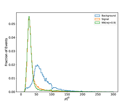
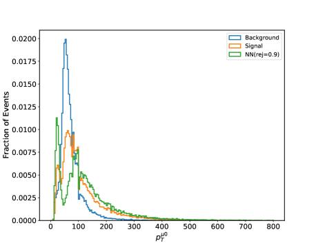
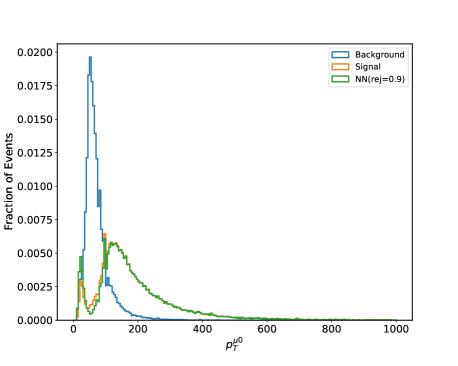
Figure 22: As in Fig. 18, except that now the $p_{T}$ distribution of the muon with the largest transverse momentum is shown.

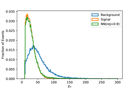
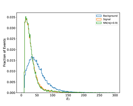
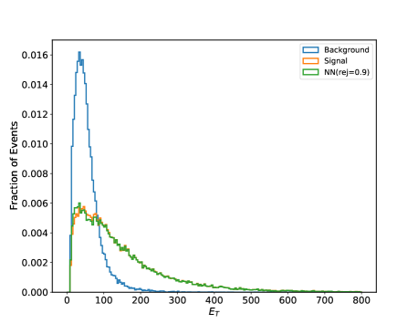
Figure 23: As in Fig. 18, except that now the missing $E_{T}$ distribution is shown.

References

- [1] X. G. He, Girish C. Joshi, H. Lew, and R. R. Volkas. New Phenomenology. Phys. Rev., D43:22–24, 1991.
- [2] T. Aoyama et al. The anomalous magnetic moment of the muon in the Standard Model. Phys. Rept., 887:1–166, 2020.
- [3] B. Abi et al. Measurement of the Positive Muon Anomalous Magnetic Moment to 0.46 ppm. Phys. Rev. Lett., 126(14):141801, 2021.
- [4] Kento Asai, Koichi Hamaguchi, and Natsumi Nagata. Predictions for the neutrino parameters in the minimal gauged U(1) model. Eur. Phys. J. C, 77(11):763, 2017.
- [5] Kento Asai, Koichi Hamaguchi, Natsumi Nagata, Shih-Yen Tseng, and Koji Tsumura. Minimal Gauged U(1) Models Driven into a Corner. Phys. Rev. D, 99(5):055029, 2019.
- [6] Anirban Biswas, Sandhya Choubey, and Sarif Khan. Neutrino Mass, Dark Matter and Anomalous Magnetic Moment of Muon in a Model. JHEP, 09:147, 2016.
- [7] Manuel Drees, Meng Shi, and Zhongyi Zhang. Constraints on from LHC Data. Phys. Lett. B, 791:130–136, 2019.
- [8] J. P. Lees et al. Search for a muonic dark force at BABAR. Phys. Rev., D94(1):011102, 2016.
- [9] D. Geiregat et al. First observation of neutrino trident production. Phys. Lett., B245:271–275, 1990.
- [10] S. R. Mishra et al. Neutrino tridents and interference. Phys. Rev. Lett., 66:3117–3120, 1991.
- [11] Wolfgang Altmannshofer, Stefania Gori, Maxim Pospelov, and Itay Yavin. Neutrino Trident Production: A Powerful Probe of New Physics with Neutrino Beams. Phys. Rev. Lett., 113:091801, 2014.
- [12] Albert M Sirunyan et al. Search for an gauge boson using Z events in proton-proton collisions at 13 TeV. Phys. Lett. B, 792:345–368, 2019.
- [13] Keisuke Harigaya, Takafumi Igari, Mihoko M. Nojiri, Michihisa Takeuchi, and Kazuhiro Tobe. Muon and LHC phenomenology in the gauge symmetric model. JHEP, 03:105, 2014.
- [14] Fatemeh Elahi and Adam Martin. Constraints on interactions at the LHC and beyond. Phys. Rev., D93(1):015022, 2016.
- [15] Eung Jin Chun, Arindam Das, Jinsu Kim, and Jongkuk Kim. Searching for flavored gauge bosons. JHEP, 02:093, 2019. [Erratum: JHEP 07, 024 (2019)].
- [16] Johan Alwall, Michel Herquet, Fabio Maltoni, Olivier Mattelaer, and Tim Stelzer. Madgraph 5: going beyond. Journal of High Energy Physics, 2011(6):1–40, 2011.
- [17] Pierre Baldi, Peter Sadowski, and Daniel Whiteson. Searching for Exotic Particles in High-Energy Physics with Deep Learning. Nature Commun., 5:4308, 2014.
- [18] Torbjörn Sjöstrand, Stefan Ask, Jesper R Christiansen, Richard Corke, Nishita Desai, Philip Ilten, Stephen Mrenna, Stefan Prestel, Christine O Rasmussen, and Peter Z Skands. An introduction to pythia 8.2. Comp. Phys. Commun., 191:159–177, 2015.
- [19] Manuel Drees, Herbi Dreiner, Daniel Schmeier, Jamie Tattersall, and Jong Soo Kim. CheckMATE: Confronting your Favourite New Physics Model with LHC Data. Comput. Phys. Commun., 187:227–265, 2015.
- [20] Daniel Dercks, Nishita Desai, Jong Soo Kim, Krzysztof Rolbiecki, Jamie Tattersall, and Torsten Weber. CheckMATE 2: From the model to the limit. Comput. Phys. Commun., 221:383–418, 2017.
- [21] J. de Favereau, C. Delaere, P. Demin, A. Giammanco, V. Lemaitre, A. Mertens, and M. Selvaggi. DELPHES 3, A modular framework for fast simulation of a generic collider experiment. JHEP, 02:057, 2014.
- [22] Matteo Cacciari, Gavin P. Salam, and Gregory Soyez. FastJet User Manual. Eur. Phys. J., C72:1896, 2012.
- [23] Matteo Cacciari and Gavin P. Salam. Dispelling the myth for the jet-finder. Phys. Lett., B641:57–61, 2006.
- [24] Matteo Cacciari, Gavin P. Salam, and Gregory Soyez. The anti- jet clustering algorithm. JHEP, 04:063, 2008.
- [25] Alexander L. Read. Presentation of search results: The CL(s) technique. J. Phys., G28:2693–2704, 2002. [,11(2002)].
- [26] C. G. Lester and D. J. Summers. Measuring masses of semiinvisibly decaying particles pair produced at hadron colliders. Phys. Lett., B463:99–103, 1999.
- [27] Alan Barr, Christopher Lester, and P. Stephens. m(T2): The Truth behind the glamour. J. Phys., G29:2343–2363, 2003.
- [28] Hsin-Chia Cheng and Zhenyu Han. Minimal Kinematic Constraints and m(T2). JHEP, 12:063, 2008.
- [29] Yang Bai, Hsin-Chia Cheng, Jason Gallicchio, and Jiayin Gu. Stop the Top Background of the Stop Search. JHEP, 07:110, 2012.
- [30] Daniel R. Tovey. On measuring the masses of pair-produced semi-invisibly decaying particles at hadron colliders. JHEP, 04:034, 2008.
- [31] Giacomo Polesello and Daniel R. Tovey. Supersymmetric particle mass measurement with the boost-corrected contransverse mass. JHEP, 03:030, 2010.
- [32] Konstantin T. Matchev and Myeonghun Park. A General method for determining the masses of semi-invisibly decaying particles at hadron colliders. Phys. Rev. Lett., 107:061801, 2011.
- [33] Ian Goodfellow, Yoshua Bengio, and Aaron Courville. Deep Learning. MIT Press, 2016. http://www.deeplearningbook.org.
- [34] Tianqi Chen and Carlos Guestrin. Xgboost: A scalable tree boosting system. Proceedings of the 22nd ACM SIGKDD International Conference on Knowledge Discovery and Data Mining, Aug 2016.
- [35] Jerome H Friedman. Greedy function approximation: a gradient boosting machine. Annals of statistics, pages 1189–1232, 2001.
- [36] Nitish Srivastava, Geoffrey Hinton, Alex Krizhevsky, Ilya Sutskever, and Ruslan Salakhutdinov. Dropout: A simple way to prevent neural networks from overfitting. Journal of Machine Learning Research, 15(56):1929–1958, 2014.
- [37] Sergey Ioffe and Christian Szegedy. Batch normalization: Accelerating deep network training by reducing internal covariate shift, 2015.