Terahertz magneto-optical properties of graphene hydrodynamic electron liquid

Abstract

The discovery of the hydrodynamic electron liquid (HEL) in graphene [D. Bandurin et al., Science 351, 1055 (2016) and J. Crossno et al., Science 351, 1058 (2016)] has marked the birth of the solid-state HEL which can be probed near room temperature in a table-top setup. Here we examine the terahertz (THz) magneto-optical (MO) properties of a graphene HEL. Considering the case where the magnetic length $l_{B}=\sqrt{\hbar/eB}$ is comparable to the mean-free path $l_{ee}$ for electron-electron interaction in graphene, the MO conductivities are obtained by taking a momentum balance equation approach on the basis of the Boltzmann equation. We find that when $l_{B}\sim l_{ee}$, the viscous effect in a HEL can weaken significantly the THz MO effects such as cyclotron resonance and Faraday rotation. The upper hybrid and cyclotron resonance magnetoplasmon modes $\omega_{\pm}$ are also obtained through the RPA dielectric function. The magnetoplasmons of graphene HEL at large wave-vector regime are affected by the viscous effect, and results in red-shifts of the magnetoplasmon frequencies. We predict that the viscosity in graphene HEL can affect strongly the magneto-optical and magnetoplasmonic properties, which can be verified experimentally.

I Introduction

Hydrodynamic electron liquid (HEL) is a classic and important phenomenon in physics. The viscous effect between different fluid layers in gas or liquid had been studied even before the birth of quantum mechanics Landau66 . It was found that akin to liquid and gas, the electrons in a Fermi-liquid can also exhibit features of hydrodynamics Baym91 , where the effect of viscosity is induced by many-body interactions in different electronic layers. The viscous effect in an electron gas system contributes an extra resistance in additional to scattering from impurities and phonons. Previously, HELs were observed mainly in the realm of high-energy physics such as quark-gluon plasma at very high temperatures Jacak12 and atomic Fermi gasses at very low temperatures Elliott14 . Since its discovery, graphene has attracted lots of attention due to its unique and novel physical properties Novoselov04 . In particular, in 2016 two research teams demonstrated experimentally that the solid-state HEL can be realized in graphene under certain conditions Bandurin16 ; Crossno16 and that it is an excellent material to investigate hydrodynamic flow of electrons.

Such important and exciting findings have marked the birth of a new subfield of solid-state HEL from which one can explore the new physics of HEL near room temperature in a table-top setup. Up to now, the solid-state HELs have been probed experimentally by using mainly transport measurements Bandurin16 ; Crossno16 ; Lucas18 ; Ku20 . One of the major advantages for a solid-state HEL is that we can employ optical techniques, which are contact-less and nondestructive, to study and characterize the hydrodynamic properties of a HEL. For an electron liquid to show hydrodynamic behavior, it is crucial that the electron-electron (e-e) interactions are significant Torre15 , which means that the mean-free path induced by electron-electron interaction, $l_{ee}$, should satisfy $l_{\mathrm{ee}}<l_{\mathrm{s}}$, $L$, and $l_{\mathrm{ee}}<v_{\mathrm{F}}/\omega$ Principi16 , for transport and optical measurements, respectively. Here, $L$ is the dimension of the sample, $l_{s}$ corresponds to the mean-free path caused by electronic scattering centers such as phonons and impurities, $v_{\mathrm{F}}=10^{6}$ m/s is the Fermi velocity of graphene, and $\omega$ is the radiation photon frequency. In a graphene-based HEL, $l_{\mathrm{ee}}$ can be smaller than 0.1 $\mu$m Bandurin16 , $L$ can be easily of the order of millimeters and $l_{s}$ can be of the order of $\mu$m Mayorov11 . Therefore, it is no surprise that graphene can be taken as the platform to probe the HEL via transport measurements Bandurin16 ; Crossno16 . It should be noticed that the above relation limits the range of validity for hydrodynamic description of a HEL to the low-frequency range. Thanks to the availability of terahertz (THz) technology Lee08 , one can employ the THz technique such as THz time-domain spectroscopy (TDS) Lee08 to probe and study the viscosity and its frequency dependence by means of optical experiments. When $\omega\sim 1$ THz, $v_{\mathrm{F}}/\omega\sim\mu$m so that the condition required for the optical measurement of graphene-based HEL can be satisfied. From a physics viewpoint, to probe the viscosity in a HEL we rely on the excitation and absorption of plasmons in graphene, which is a direct consequence of e-e interaction. It is known that in the absence of a magnetic field $B$, the optical conductivity for an electron gas in the presence of viscosity can be written simply as Principi16

$$\sigma(q,\omega)={\sigma_{0}\over 1-i\omega\tau+\nu q^{2}\tau},$$ (1)

where $\omega_{\nu}=\nu q^{2}$ is the characteristic frequency for a HEL and we call it the viscous frequency, $\sigma_{0}=e^{2}n_{e}v_{\mathrm{F}}\tau/(\hbar k_{\mathrm{F}})$ is the dc conductivity of graphene at $B=0$, $n_{e}$ is the electron density, $\tau$ is the electronic momentum relaxation time, $\nu$ is the viscosity, $q$ is the wave vector of elementary electronic excitation induced via e-e interaction and $k_{\mathrm{F}}=\sqrt{\pi n_{e}}$ is the Fermi wave vector for graphene. From Eq. (1), we learn that only excitations with a non-zero momentum $q$ are sensitive to viscosity-induced relaxation in optical measurement.

Recently, the study of the optoelectronic properties of graphene in the presence of a magnetic field was presented such as the Landua levels, cyclotron resonance, Faraday rotation, ellipticity, and magnetoplasmons Jiang07 ; Tymchenko13 ; Crassee12 ; Yan12 . In the presence of a static magnetic field applied perpendicularly to the graphene flake, plasmons and cyclotron excitations would hybridize which can lead to the formation of magnetoplasmons. In 2D electron gas, the magneto plasmon has a dispersion relation $\omega^{2}=\omega^{2}_{c}+\omega^{2}_{p}$ which is called the upper hybrid mode Ando82 ; Roldan09 where $\omega_{c}$ and $\omega_{p}$ are cyclotron frequency and plasmon frequency, respectively. It has been shown that the viscosity of graphene-based electron liquid is of the order of $\nu\approx$ 0.1 m²s^-1 Bandurin16 . In the presence of magnetic field, the off-diagonal part of viscous response coefficient is called Hall viscosity. The Hall viscosity in graphene has been measured Berdyugin19 and it is smaller than the kinetic viscosity at relatively weak magnetic field Narozhny19 . By the way, the Hall viscosity is also the coefficient of $q^{2}$ in the small-$q$ limit Sherafati19 . Thus, in this study we only consider the effect of the kinetic viscosity. From Eq. (1), we see that the viscosity in graphene HEL would affect the optical conductivity at different finite wavevector $q$. We predict that the viscosity can also affect the magneto-optical properties of graphene HEL. The viscosity effect in the presence of magnetic field can be probed via THz magneto-optical measurements Mei18 ; wxu2 .

In this work, we examine the magneto-optical (MO) properties of a graphene-based HEL. Our approach is developed on the basis of a semi-classic Boltzmann equation and random phase approximation (RPA). We will present and discuss the results obtained for the magneto-optical conductivity, Faraday rotation angle and ellipticity, and the magneto-plamson modes of a graphene HEL.

II Theoretical approach

In this study, we consider the case of a relatively weak magnetic field which does not induce Landau quantization and the corresponding magnetic length $l_{B}=\sqrt{\hbar/eB}$ is comparable to $l_{ee}$ in graphene. We employ the semi-classic Boltzmann equation (BE) approach to evaluate the MO conductivity of a graphene-based HEL in the presence of the viscosity effect. Recently, the electronic hydrodynamics in graphene has been investigated in detail on the basis of the kinetic theory to obtain the generalized Navier-Stokes equation and the explicit expressions for the shear and Hall viscosity Narozhny19Rev . In this theoretical work Narozhny19Rev , a two-band model has been used for arbitrary doping levels of graphene where the infinite number of particles in the filled band were considered. In the present study, we consider the case where the conducting carriers are only electrons and take the viscous effect as an input parameter to show how it would affect the magneto-optical properties of a graphene hydrodynamics system. Here, high quality samples are considered and the electrons are distributed uniformly in the graphene film. Moreover, the temperature is uniform and the chemical potential can be tuned via, e.g., applying a gate voltage. In the presence of a weak radiation field, we assume the spatial inhomogeneities of the distribution can be safely ignored due to fast relaxation processes via, e.g., the electron-electron (e-e) scattering which occurs in homogenous scattering centers. For simplification of our model, the distribution function therefore would not depend on spatial coordinate since the temperature and the chemical potential for the system are with no gradients. The time-dependent semiclassic BE Xu97 for the homogeneous electrons in conduction band of graphene is given as

$${1\over\hbar} [{\bf F}_{1}(t)+{\bf F}_{2}(t)]\nabla_{\bf k}f_{e}({\bf k},t)+{\partial f_{e}({\bf k},t)\over\partial t}$$

$$=g_{s}g_{v}\sum_{{\bf k}^{\prime}}[F({\bf k}^{\prime},{\bf k};t)-F({\bf k},{\bf k}^{\prime};t)],$$ (2)

where ${\bf k}=(k_{x},k_{y})$ is the electron wave vector, $f_{e}({\bf k},t)$ is the momentum distribution function (MDF) for an electron in a state $|{\bf k}\rangle$ and at a time $t$, $g_{s}=2$ and ${\it g_{v}}=2$ count respectively for spin and valley degeneracies, and $F({\bf k},{\bf k^{\prime}};t)=f_{e}({\bf k},t)W({\bf k},{\bf k^{\prime}})$ is the collision term induced by electronic scattering centers with $W({\bf k},{\bf k^{\prime}})$ being the electronic transition rate. Moreover, the force term here includes two contributions from, respectively, the applied external field ${\bf F}_{1}(t)$ and the frictional force Kubo92 : ${\bf F}_{2}(t)=-\gamma q^{2}{\bf v}(t)$ with ${\bf v}(t)=[v_{x}(t),v_{y}(t)]$ being the electron drift velocity which also depends little on spatial coordinate in a homogeneous graphene system, with $q$ being the wave vector of the elementary electronic excitation via e-e interaction and $\gamma$ the viscosity coefficient. We consider that the HEL is subjected simultaneously to a linearly polarized radiation field and a static magnetic field $B$ in the Faraday geometry. Namely, the magnetic and radiation fields are applied perpendicularly to the 2D plane (taken as the $xy$-plane) of the graphene flake and the polarization of the light field is taken along the $x$-direction. In this geometry, due to the coupling of the magnetic and radiation fields, the effects of cyclotron resonance and the rotation of the light polarization by the HEL can be observed. We can write the electric field component of the radiation field as ${\bf E}(t)=F_{0}(1,0,0)e^{-i\omega t}$ and the magnetic field as ${\bf B}=(0,0,B)$ and, thus, ${\bf F}_{1}(t)=-e{\bf E}(t)-e{\bf v}(t)\times{\bf B}$. Equation (II) along the $[x,y]$ direction then becomes

$$-{1\over\hbar}\Big{[} A_{x}(t){\partial f_{e}({\bf k},t)\over\partial k_{x}},A_{y}(t){\partial f_{e}({\bf k},t)\over\partial k_{y}}\Big{]}+{\partial f_{e}({\bf k},t)\over\partial t}$$

$$=g_{s}g_{v}\sum_{{\bf k}^{\prime}}[F({\bf k}^{\prime},{\bf k};t)-F({\bf k},{\bf k}^{\prime};t)],$$ (3)

with $A_{x}(t)=eF_{0}e^{-i\omega t}+eBv_{y}(t)+\gamma q^{2}v_{x}(t)$ and $A_{y}(t)=-eBv_{x}(t)+\gamma q^{2}v_{y}(t)$. For the first moment, the momentum-balance equation (MBE) can be derived by multiplying $g_{s}g_{v}\sum_{\bf k}k_{\alpha}$ to both sides of the BE given by Eq. (II), where $\alpha=(x,y)$. It should be noted that the main effect of ${\bf F}_{1}(t)$ is to cause a drift velocity ${\bf v}(t)$ of the electron in a HEL. As a result, the electron wave vector in the MDF is shifted by Xu05 ; Xu91 ; Xu09 ${\bf k}\to{\bf k}^{*}(t)={\bf k}-(k_{\mathrm{F}}/v_{\mathrm{F}}){\bf v}(t)$. Thus, the MBE derived from the BE becomes

$${n_{e}k_{\mathrm{F}}\over v_{\mathrm{F}}}\dot{v}_{\alpha}(t)+{n_{e}\over\hbar}A_{\alpha}(t)=16\sum_{{\bf k}^{\prime},{\bf k}}(k_{\alpha}^{\prime}-k_{\alpha})f_{e}[{\bf k}^{*}(t)]W({\bf k},{\bf k}^{\prime}),$$ (4)

where $n_{e}=g_{s}g_{v}\sum_{\bf k}f_{e}({\bf k})$ and the dependence of the MDF on time is mainly through the velocity ${\bf v}(t)$. For the case of a relatively weak radiation field $E(t)$, the drift velocity of the electron is relatively small so that we can make use of the expansion

$$f_{e}[{\bf k}^{*}(t)]\simeq f_{e}({\bf k})-{k_{\mathrm{F}}\over v_{\mathrm{F}}}\big{[}v_{x}(t){\partial f_{e}({\bf k})\over\partial k_{x}},v_{y}(t){\partial f_{e}({\bf k})\over\partial k_{y}}\big{]}.$$ (5)

Due to the symmetry of the electronic energy spectrum of graphene, i.e., $E({\bf k})=\hbar v_{\mathrm{F}}k$, we have $\sum_{{\bf k}^{\prime},{\bf k}}(k_{\alpha}^{\prime}-k_{\alpha})f_{e}({\bf k})W({\bf k},{\bf k}^{\prime})=0$ and, therefore, we have

$${\partial v_{\alpha}(t)\over\partial t}+{v_{\mathrm{F}}A_{\alpha}(t)\over\hbar k_{\mathrm{F}}}=-{v_{\alpha}(t)\over\tau},$$ (6)

where the momentum relaxation time is determined by

$${1\over\tau}={16\over n_{e}}\sum_{{\bf k}^{\prime},{\bf k}}(k_{\alpha}^{\prime}-k_{\alpha})W({\bf k},{\bf k}^{\prime}){\partial f_{e}({\bf k})\over\partial k_{\alpha}},$$ (7)

in which the temperature dependence is included in the electron distribution function and in the electronic scattering mechanisms. The momentum relaxation time is contributed from electronic scattering centers such as impurities, phonons, surface roughness, etc. In our previous work Dong08 ; Xu09 , by using the momentum-balance equation approach on the basis of the BE at $B=0$ we had discussed the temperature dependence of the carrier density and the transport lifetime (or momentum relaxation time) in graphene. The obtained theoretical results reproduced the experimental results measured via transport experiment Bandurin16 since the DC conductivity is given by $\sigma_{0}=e^{2}n_{e}v_{\mathrm{F}}\tau/(\hbar k_{\mathrm{F}})$. Furthermore, if we take the MDF $f_{e}({\bf k})$ in Eq. (7) to be approximately as the statistical electron energy distribution function such as the Fermi-Diraction through: $f_{e}({\bf k})\simeq f_{e}[E({\bf k})]$ with $f_{e}(x)$ being the Fermi-Dirac function, the dependence of $\tau$ upon the temperature and chemical potential can be further included. For weak radiation field $E(t)=F_{0}e^{-i\omega t}$, the electrons in graphene respond linearly to the radiation so that $v_{\alpha}(t)=v_{\alpha}e^{-i\omega t}$. Thus, we can get the steady-state electron drift velocity ${\bf v}=(v_{x},v_{y})$ and the current density ${\bf J}=-n_{e}e{\bf v}$. After applying the current-voltage matrix ${\bf J}=\sigma{\bf E}$ with $\sigma$ being the conductivity tensor and ${\bf E}=F_{0}(1,0,0)$, the longitudinal and transverse MO conductivities of HEL are obtained as, respectively,

$$\sigma_{xx}(q,\omega)=\sigma_{0}{1+\omega_{v}\tau-i\omega\tau\over(1+\omega_{\nu}\tau-i\omega\tau)^{2}+(\omega_{c}\tau)^{2}},$$ (8)

$$\sigma_{xy}(q,\omega)=-\sigma_{0}{\omega_{c}\tau\over(1+\omega_{\nu}\tau-i\omega\tau)^{2}+(\omega_{c}\tau)^{2}},$$ (9)

where $\omega_{c}=eBv_{\mathrm{F}}/(\hbar k_{\mathrm{F}})$ is the cyclotron frequency of graphene and $\omega_{\nu}=\gamma q^{2}v_{\mathrm{F}}/(\hbar k_{\mathrm{F}})$. If we write $\omega_{\nu}=\nu q^{2}$, then effective viscosity for a graphene HEL is $\nu=\gamma k_{\mathrm{F}}/(\hbar v_{\mathrm{F}})\sim n_{e}^{1/2}$. When $B=0$, $\sigma_{xy}(\omega)=0$ and $\sigma_{xx}(\omega)=\sigma(\omega)$, as given by Eq. (1).

From $\sigma_{xx}(q,\omega)$ and $\sigma_{xy}(q,\omega)$, we can obtain the right-handed circular (RHC) and left-handed circular (LHC) MO conductivities via Palik70

$$\sigma_{\pm}(q,\omega)=\sigma_{xx}\pm i\sigma_{xy}={\sigma_{0}\over 1+\omega_{\nu}\tau-i(\omega\mp\omega_{c})\tau}.$$ (10)

Now we look at the experimental aspects of the measurement by using THz TDS technique. In a conventional THz TDS setup Mei18 the THz radiation is normally linearly polarized. One often applies the linear polarizer to measure the transmission coefficients at polarization angles $\pm 45^{o}$ to the polarization direction of the incident THz beam Mei18 . If the electric field component of the THz beam transmitted through the sample (graphene/substrate) or the substrate is $E_{\pm 45^{o},j}(\omega)$ with $j$ representing the result measured for the sample or the substrate, then the corresponding right-hand circularly (RHC) and left-hand circularly (LHC) polarized light fields can be obtained according to Fresnel theory Morikawa06 ,

$$\left[\begin{array}[]{cc}E_{+,j}(\omega)\\ E_{-,j}(\omega)\end{array}\right]={1\over 2}\left(\begin{array}[]{cc}i-1&i+1\\ i+1&i-1\end{array}\right)\times\left[\begin{array}[]{cc}E_{+45^{\mathrm{o}},j}(\omega)\\ E_{-45^{\mathrm{o}},j}(\omega)\end{array}\right].$$ (11)

Thus, the transmission coefficients of the RHC and LHC components for graphene HEL can be determined by

$$t_{\pm}(\omega)=E_{\pm,\mathrm{sample}}(\omega)/E_{\pm,\mathrm{substrate}}(\omega).$$ (12)

The relationship between the transmission coefficients of the RHC and LHC components and the RHC and LHC conductivities is Chiu76

$$t_{\pm}(\omega)={2n_{0}\over n_{0}+n_{s}+Z_{0}\sigma_{\pm}(q,\omega)}=|t_{\pm}(\omega)|e^{i\zeta_{\pm}(\omega)},$$ (13)

where $n_{0}=3.6$ and $n_{s}=2.2$ are the indices of refraction of the substrate and graphene respectively, $Z_{0}\approx 377\ \Omega$ is the impedance of free space, and $|t_{\pm}(\omega)|$ and $\zeta_{\pm}(\omega)$ are the module and the phase angle of the transmission coefficient, respectively. It should be noted that the presence of the dielectric substrate may influence the hydrodynamic regime in graphene. It was shown that graphene on hexagonal boron nitride (h-BN) substrate can have electronic mobility and carrier inhomogeneity that are almost an order of magnitude better than devices on SiO₂ substrate Dean10 ; Mayorov11 . To minimize the disorder for sustaining hydrodynamic regime, the graphene film is usually encapsulated between the h-BN crystals for experimental settings Bandurin16 ; Berdyugin19 ; Crossno16 .

The Faraday rotation angle $\theta(\omega)$ and the ellipticity $\eta(\omega)$ are related to the transmission coefficients through OConnell82

$${t_{-}(\omega)\over t_{+}(\omega)}={1-\eta(\omega)\over 1+\eta(\omega)}e^{-2i\theta(\omega)}.$$ (14)

Therefore, we obtain the Faraday rotation angle

$$\theta(\omega)={1\over 2}[\zeta_{+}(\omega)-\zeta_{-}(\omega)]={1\over 2}\tan^{-1}\frac{r(b_{-}d_{+}-d_{-}b_{+})}{r^{2}b_{-}b_{+}+d_{-}d_{+}},$$ (15)

where $a=1+\omega_{v}\tau$, $b_{\pm}=(\omega\mp\omega_{c})\tau$, $r=Z_{0}\sigma_{0}/(n_{0}+n_{s})$, and $d_{\pm}=(a^{2}+b_{\pm}^{2}+ra)$. Meanwhile, the ellipticity is given by

$$\eta(\omega)={|t_{+}(\omega)|-|t_{-}(\omega)|\over|t_{+}(\omega)|+|t_{-}(\omega)|}=\frac{c_{+}f_{-}-c_{-}f_{+}}{c_{-}f_{+}+c_{+}f_{-}},$$ (16)

where $c_{\pm}=a^{2}+b_{\pm}^{2}$ and $f_{\pm}=\sqrt{d_{\pm}^{2}+r^{2}b_{\pm}^{2}}$.

Furthermore, the longitudinal conductivity has a direct relation to the density-density correlation function $\sigma_{xx}(q,\omega)=ie^{2}\omega\chi_{nn}(q,\omega)/q^{2}$. The random-phase approximation (RPA) dielectric function can be written as Giuliani05

$$\epsilon_{\mathrm{RPA}}(q,\omega)=1-v_{q}\chi_{nn}(q,\omega)=1+\frac{iq^{2}v_{q}}{e^{2}\omega}\sigma_{xx}(q,\omega),$$ (17)

The magneto-plasmons can then be obtained by the real roots for the zeros of the real part of the dielectric function $\mathrm{Re}\ \epsilon_{\mathrm{RPA}}(q,\omega)\rightarrow 0$. The imaginary part of $\epsilon_{\mathrm{RPA}}(q,\omega)$ relates directly the decay or damping of the electronic motion. Thus, we obtain two branches of the plasmon modes as

$$\omega^{2}_{\pm}=\omega^{2}_{c}+\frac{\omega_{p}^{2}}{2}-(\tau^{-1}+\nu q^{2})^{2}\pm\sqrt{\frac{\omega_{p}^{4}}{4}-4\omega_{c}^{2}(\tau^{-1}+\nu q^{2})^{2}},$$ (18)

where $\omega_{p}=\sqrt{e^{2}E_{\mathrm{F}}q/(2\pi\epsilon_{r}\epsilon_{0})}$ is the Dirac plasmon frequency of graphene.

III Results and discussions

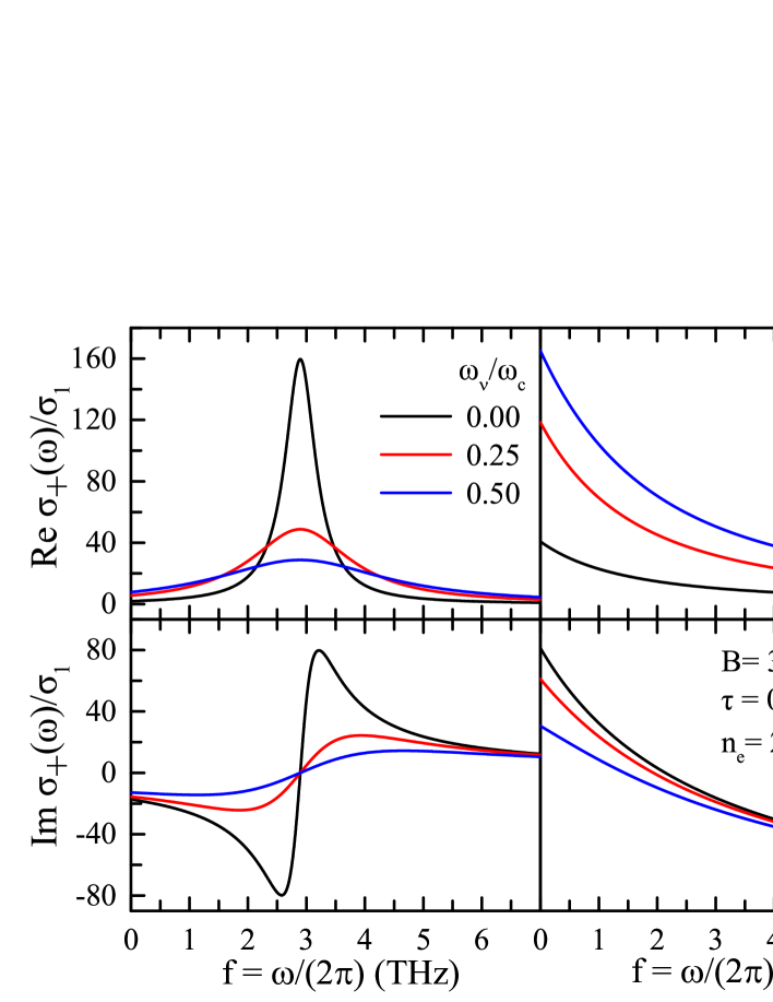
Figure 1: Theoretical spectra of the real and imaginary parts of the RHC and LHC MO conductivities, $\sigma_{\pm}(\omega)$, as a function of radiation frequency $f=\omega/(2\pi)$ at the fixed magnetic field, electron density and electronic relaxation time for different viscous frequencies. Here, the optical conductivity is in an unit of $\sigma_{1}=e^{2}/4\hbar$.

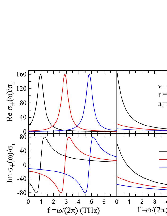
Figure 2: The real and imaginary parts of the RHC and LHC MO conductivities, $\sigma_{\pm}(\omega)$, as a function of radiation frequency $f=\omega/(2\pi)$ at the fixed viscosity with wave vector $q=3\times 10^{5}$ cm^-1, electron density and electronic relaxation time for different magnetic field strengths.

For numerical calculations, we use the typical carrier density with the order $n_{e}\sim 10^{12}$ cm^-2 for a “higher-than-in-hone” viscosity $\nu\approx$ 0.1 m²s^-1 Bandurin16 ; Narozhny19 at a temperature $T=220$ K. Ho and coworkers reported Ho18 that a large and robust hydrodynamic window exists in graphene over a wide range of carrier density deviation from charge neutrality and temperatures from 150 to 300 K, where the e-e interaction is the dominant scattering mechanism and it can support both the plasmon and single-carrier hydrodynamic regimes. In the presence of viscous effect in a graphene HEL, the effect of viscosity on the optical conductivity and plasmon should relative to a finite wave vector $q$. In terms of spectroscopic measurement, such a momentum mismatch can be realized through, e.g., patterning the gratings on graphene film Wenger16 which has been realized experimentally for the observation of the HEL effect in graphene Maier07 ; Zhu13 ; Jadidi15 .

In conjunction with the MO THz TDS measurement, in Fig. 1 we plot the real and imaginary parts of the RHC and LHC conductivities, $\sigma_{\pm}(\omega)$, as a function of radiation frequency $f=\omega/2\pi$ at the fixed magnetic field $B=3$ T with a typical electron density $n_{e}=2\times 10^{12}$ cm^-2 for different viscous frequencies $\omega_{\nu}$. For the calculation, we take a typical electronic relaxation time $\tau=0.5$ ps. We note that, with the Drude-like MO conductivity as used in this study, the temperature dependence is included in the momentum relaxation time given by Eq. (7) since $\tau$ is a functional form of the carrier density and temperature. The increase in temperature can lead to a decrease in $\tau$ in graphene system due mainly to the electron-phonon scattering Bandurin16 ; Dong08 . The temperature dependence of $\tau$ can be determined through transport measurement and the corresponding values can be included in the evaluation of the viscosity effect. Similar to other electron gas systems OConnell82 , the cyclotron resonance can be observed in the real and imaginary parts of $\sigma_{+}(\omega)$ when $\omega\sim\omega_{c}$. From Fig. 1, we find that the real and imaginary parts of $\sigma_{\pm}(\omega)$ decrease with increasing viscous frequency $\omega_{\nu}$ or the strength of the viscosity. This effect is akin to the case of transport experiments for a HEL in which an extra resistance is added to the total resistance in additional to that induced by electronic scattering from impurities and phonons Pellegrino17 . In Fig. 2, we show the real and imaginary parts of RHC and LHC conductivities as a function of radiation frequency at the fixed viscous frequency, electron density $n_{e}=2\times 10^{12}$ cm^-2 for different magnetic fields. The real and imaginary parts of RHC conductivities blueshift with increasing magnetic field while the strength of LHC conductivities decrease with increasing $B$. In Fig. 3 we present the corresponding Faraday ellipticity $\eta(\omega)$ and rotation angle $\theta(\omega)$ as a function of radiation frequency at the fixed magnetic field, electron density and electronic relaxation time for different viscous frequencies $\omega_{\nu}$. We find, again, that both $\eta(\omega)$ and $\theta(\omega)$ decrease with increasing $\omega_{\nu}$. Therefore, the viscosity can weaken the magneto-optical absorption in a graphene HEL.

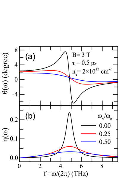
Figure 3: Spectra of (a) the Faraday rotation angle $\theta(\omega)$ and (b) the Faraday ellipticity $\eta(\omega)$ as a function of radiation frequency $f=\omega/(2\pi)$ at the fixed magnetic field, electron density and electronic relaxation time for different viscous frequencies.

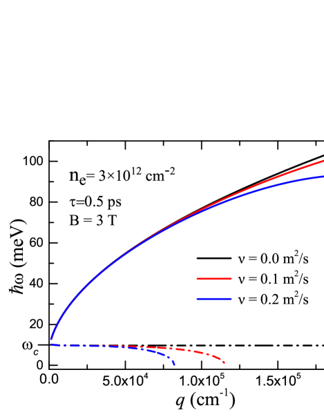
Figure 4: The magneto-plasmon energy of a graphene HEL as a function of wave vector $q$ at the fixed electron density and magnetic field for different viscosities. The solid and dash-dotted curves denote the upper hybrid mode $\omega_{+}$ and the cyclotron resonance mode $\omega_{-}$, respectively.

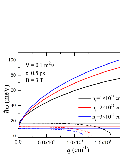
Figure 5: The magnetoplasmon energy of a graphene HEL as a function of wave vector $q$ at the fixed viscosity and magnetic field for different electron densities. The solid and dash-dotted curves denote the upper hybrid mode $\omega_{+}$ and the cyclotron resonance mode $\omega_{-}$, respectively. The translucence solid horizonal lines are the cyclotron frequencies for the corresponding cyclotron resonant modes.

In Fig. 4 we plot the magnetoplasmon energy as a function of wave vector $q$ at the fixed electron density, magnetic field strength for different viscosities. Notice, there are two magnetoplasmon branches corresponding to the upper hybrid mode $\omega_{+}$ and the cyclotron resonance mode $\omega_{-}$. In the absence of viscosity $\nu=0$, the upper hybrid mode $\omega_{+}\simeq\sqrt{\omega^{2}_{c}+\omega^{2}_{p}}$ Ando82 and the cyclotron resonance mode $\omega_{-}\simeq\omega_{c}$ corresponds to the cyclotron resonance frequency. In the collisionless limit (i.e., $\tau\rightarrow\infty$), the $\omega_{-}$ mode vanishes in the small $q$ regime and only the $\omega_{+}$ mode exists Volkov16 . The magnetoplasmon frequencies of the upper hybrid mode and cyclotron resonance mode at large $q$ decrease with increasing viscosity. When the viscosity $\nu\neq 0$, the cyclotron resonance mode decreases with increasing $q$ and approaches to zero at a cutoff wave vector. This mode with a frequency below $\omega_{c}$ attributes to the friction force which can slow down the electron movement owing to the e-e interaction in the presence of the viscosity. The magnetoplasmon dispersion at the fixed magnetic field strength, viscosity for different electron densities is shown in Fig. 5. The cyclotron frequency of graphene $\omega_{c}=eBv_{\mathrm{F}}/(\hbar k_{\mathrm{F}})$ depends on the Fermi wave vector $k_{\mathrm{F}}$. Thus, $\omega_{c}$ decreases with increasing carrier density. With increasing the carrier density, the magnetoplasmon frequency of the upper hybrid mode is higher and the cyclotron resonance mode becomes lower in a larger wave vector $q$ regime.

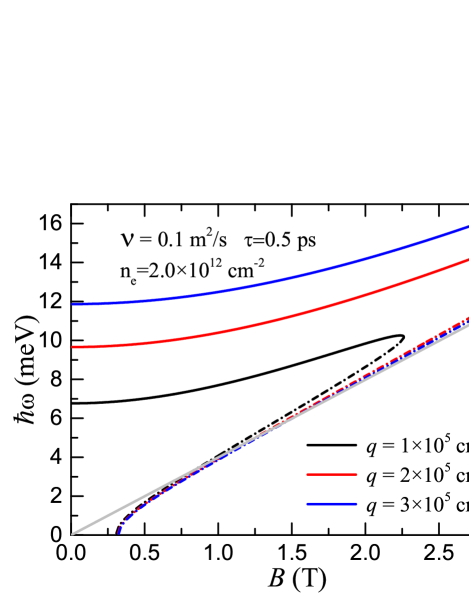
Figure 6: The magnetoplasmon modes of a graphene HEL as a function of magnetic field $B$ at the fixed viscosity and electron density for different wave vectors $q$. The solid and dashed-dotted curves denote the upper hybrid mode $\omega_{+}$ and the cyclotron resonance mode $\omega_{-}$, respectively. Here, the gray line denotes the cyclotron frequency $\hbar\omega_{c}$.

In Fig. 6 we plot the magnetoplasmon energy as a function of magnetic field strength at the fixed carrier density and viscosity for different wave vectors $q$. The two magnetoplasmon frequencies increase with increasing magnetic field $B$. For a fixed wave vector $q=1\times 10^{5}$ cm^-1, the upper hybrid mode and the cyclotron resonance mode coincide at a cutoff $B$ point with increasing the magnetic field $B$. We can see that the frequency of the cyclotron resonance mode is slightly below the cyclotron frequency at small magnetic fields and higher than the cyclotron frequency at large magnetic fields. We can clearly observe that the upper hybrid mode show the $\omega_{+}\simeq\sqrt{\omega^{2}_{c}+\omega^{2}_{p}}$ dependence upon the magnetic field strength.

In recent years, the THz TDS technique has been employed to investigate into the optoelectronic properties of atomically thin electronic systems such as graphene Mei18 , monolayer (ML) MoS₂ Wang19 , ML WS₂ Dong20 , ML hBN Bilal20 , etc. It had been demonstrated experimentally Mei18 that through MO THz TDS measurement, we can obtained the spectra of the real and imaginary parts of $\sigma_{\pm}(\omega)$ or $\sigma_{xx}(\omega)$ and $\sigma_{xy}(\omega)$. The magnetoplasmon resonances could also be probed by a variety of methods such as electron energy-loss spectroscopy, inelastic light scattering, angle-resolved photoemission spectroscopy (ARPES), scanning tunnelling spectroscopy Grigorenko12 , etc. From our theoretical calculation, the viscousity in graphene-based HEL weakens the optical conductivity and affects the magnetoplasmon properties at large wave vector $q$.

IV Conclusions

In this work, we consider a relatively weak magnetic field such that it does not induce the Landau quantization and the magnetic length $l_{B}$ is comparable to $l_{ee}$ in graphene. In such a case, the cyclotron resonance induced by intra-band electronic transition can be observed in the MO conductivity and the Faraday rotation in THz frequency regime. Because $l_{B}\sim l_{ee}$, the presence of viscosity in a HEL can weaken significantly these characteristic MO effects. We have investigated the magnetoplasmon modes in graphene HEL in which an upper hybrid mode and a cyclotron resonance mode exist. Both two modes are affected strongly by the viscous effect in the large wave vector regime. The magnetoplasmon frequency of the cyclotron resonance mode decreases and approaches to zero with decreasing wave vector. From the results obtained for a relatively weak magnetic field, one can expect that the magnetoplasmon effect occur at relatively large wave vector regime and exhibit a frequency shift caused by the viscosity, especially the $\omega_{-}$ mode which can be below the cyclotron resonance frequency $\omega_{c}$.

In summary, the recent discovery of the hydrodynamic electron liquid (HEL) in graphene has opened up a new subfield of solid-state HEL. This allows us to explore the new physics of HEL near room temperature in a table-top setup. In this work, we have studied theoretically the terahertz (THz) magneto-optical (MO) and magnetoplasmon properties of a graphene-based HEL. The present study has been focused on the situation where the magnetic length $l_{B}=\sqrt{\hbar/eB}$ is comparable to the mean-free path $l_{ee}$ for electron-electron interaction in graphene. We have obtained the longitudinal and transverse MO conductivities, $\sigma_{xx}(\omega)$ and $\sigma_{xy}(\omega)$, by using a momentum balance equation approach derived from a semiclassic Boltzmann equation in which the frictional force induced by the viscosity is included. We also obtain the right-handed circular and left-handed circular MO conductivities, $\sigma_{\pm}(\omega)$, along with the Faraday rotation angle $\theta(\omega)$ and ellipticity $\eta(\omega)$. The magneto-plasmon modes have been evaluated using the model of the RPA. The upper hybrid mode and the cyclotron resonance mode are obtained and examined.

In conjunction to the MO THz TDS measurement, we have examined the dependence of the spectra of the real and imaginary parts of $\sigma_{\pm}(\omega)$, along with $\theta(\omega)$ and $\eta(\omega)$, on the viscous frequency. It has been found that the viscous effect in a HEL can weaken significantly the THz MO effects such as the cyclotron resonance and the Faraday rotation. The magnetoplasmon modes in graphene HEL in the large wave vector regime are affected a lot by the viscous effect, especially the red-shifts of the magnetoplasmon frequency can be observed. We hope that the theoretical prediction in this study can be verified experimentally and deepen our understanding of the magneto-optical properties of graphene-based HEL.

References

- (1) L. D. Landau, E. M. Lifshitz, Course of Theoretical Physics: Fluid Mechanics (Pergamon, New York, 1966).
- (2) G. Baym and G. Pethick, Landau Fermi-Liquid Theory: Concepts and Applications (John Wiley Sons, New York,, 1991).
- (3) B. V. Jacak and B. Müller, Science 337, 310-314 (2012).
- (4) E. Elliott, J.A. Joseph, and J.E. Thomas, Phys. Rev. Lett. 113, 020406 (2014).
- (5) K. S. Novoselov, A. K. Geim, S. V. Morozov, D. Jiang, Y. Zhang, S. V. Dubonos, I. V. Grigorieva, A. A. Firsov, Science 306, 666 (2004).
- (6) D. A. Bandurin, I. Torre, R. K. Kumar, M. B. Shalom, A. Tomadin, A. Principi, G. H. Auton, E. Khestanova, K. S. Novoselov, and I. V. Grigorieva, Science 351, 1055 (2016).
- (7) J. Crossno, J. K. Shi, K. Wang, Xiaomeng Liu, A. Harzheim, A. Lucas, S. Sachdev, P. Kim, T. Taniguchi, K. Watanabe, T. A. Ohki, and K. C. Fong, Science 351, 1058 (2016).
- (8) A. Lucas, and K. C. Fong, J. Phys: Condens. Matter. 30, 053001 (2018).
- (9) M. J. H. Ku, T. X. Zhou, Q. Li, Y. J. Shin, J. K. Shi, C. Burch, L. E. Anderson, A. T. Pierce, Y. Xie, A. Hamo, U. Vool, H. Zhang, F. Casola, T. Taniguchi, K. Watanabe, M. M. Fogler, P. Kim, A. Yacoby, and R. L. Walsworth, Nature 583, 537 (2020).
- (10) I. Torre, A. Tomadin, A. K. Geim, and M. Polini, Phys. Rev. B 92, 165433 (2015).
- (11) A. Principi, G. Vignale, M. Carrega, and M. Polini, Phys. Rev. B 93, 125410 (2016).
- (12) A. S. Mayorov, R. V. Gorbachev, S. V. Morozov, L. Britnell, R. Jalil, L. A. Ponomarenko, P. Blake, K. S. Novoselov, K. Watanabe, T. Taniguchi, A. K. Geim, Nano Lett. 11, 2396-2399 (2011).
- (13) Y. S. Lee, Principles of Terahertz Science and Technology (Springer, New York, 2008).
- (14) Z. Jiang, E. A. Henriksen, L. C. Tung, Y.-J. Wang, M. E. Schwartz, M. Y. Han, P. Kim, and H. L. Stormer, Phys. Rev. Lett. 98, 197403 (2007).
- (15) M. Tymchenko, A. Yu. Nikitin,and L. Martín-Moreno, ACS Nano 7(11), 9780-9787 (2013).
- (16) I. Crassee, M. Orlita, M. Potemski, A. L. Walter, M. Ostler, Th. Seyller, I. Gaponenko, J. Chen, and A. B. Kuzmenko, Nano Lett. 12, 2470-2474 (2012).
- (17) H. Yan, Z. Li, X. Li, W. Zhu, P. Avouris, and F. Xia, Nano Lett. 12, 3766-3771 (2012).
- (18) T. Ando, A. B. Fowler, and F. Stern, Rev. Mod. Phys. 54, 437 (1982).
- (19) R. Roldán, J. -N. Fuchs, and M. O. Goerbig, Phys. Rev. B 80, 085408 (2009).
- (20) A. I. Berdyugin, S. G. Xu, F. M. D. Pellegrino, R. Krishna Kumar, A. Principi, I. Torre, M. Ben Shalom, T. Taniguchi, K. Watanabe, I. V. Grigorieva, M. Polini, A. K. Geim, D. A. Bandurin, Science 364, 162-165 (2019).
- (21) B. N. Narozhny, and M. Schütt, Phys. Rev. B 100, 035125 (2019).
- (22) M. Sherafati and G. Vignale, Phys. Rev. B 100, 115421 (2019).
- (23) H. Y. Mei, W. Xu, C. Wang, H. F. Yuan, C. Zhang, L. Ding, J. Zhang, C. Deng, Y. F. Wang, and F. M. Peeters, J. Phys.: Condens. Matter 30, 175701 (2018).
- (24) H. Wen, W. Xu, C. Wang, D. Song, H. Mei, J. Zhang, and L. Ding, Nano Select 2, 90-98 (2021).
- (25) B. N. Narozhny, Ann. of Phys. 411 167979 (2019).
- (26) W. Xu and C. Zhang, Phys. Rev. B 55, 5259 (1997).
- (27) R. Kubo, M. Toda, and N. Hashitsume, Statistical Physics II: Nonequilibrium Statistical Mechanics (Springer-Verlag, Berlin, 1992).
- (28) W. Xu, Phys. Rev. B. 71, 245304 (2005).
- (29) W. Xu, F. M. Peeters, and J. T. Devreese Phys. Rev. B. 43, 14134 (1991).
- (30) W. Xu, F. M. Peeters, and T. C. Lu Phys. Rev. B. 79, 073403 (2009).
- (31) H. M. Dong, W. Xu, Z. Zeng, T. C. Lu, and F. M. Peeters, Phys. Rev. B 77, 235402 (2008).
- (32) E. D. Palik and J. K. Fudrdyna, Rep. Prog. Phys. 33, 1193 (1970).
- (33) O. Morikawa, A. Quema, S. Nashima, H. Sumikura, T. Nagashima, and M. Hangyo, J. Appl. Phys. 100, 033105 (2006).
- (34) K. W. Chiu, T. K. Lee, and J. J. Quinn, Surf. Sci. 58, 182 (1976).
- (35) C. R. Dean, A. F. Young, I. Meric, C. Lee, L. Wang, S. Sorgenfrei, K. Watanabe, T. Taniguchi, P. Kim, K. L. Shepard, and J. Hone, Nat. Nanotech. 5, 722-726 (2010).
- (36) R. F. O’Connell and G. Wallace, Phys. Rev. B 26, 2231 (1982).
- (37) G. F. Giuliani and G. Vignale, Quantum Theory of the Electron Liquid (Cambridge University Press, Cambridge, UK, 2005).
- (38) D. Y. H. Ho, I. Yudhistira, N. Chakraborty, and S. Adam, Phys. Rev. B 97, 121404(R) (2018).
- (39) T. Wenger, G. Viola, and M. Fogelström, Phys. Rev. B 94, 205419 (2016).
- (40) S. Maier, Plasmonics: Fundamentals and Applications (Springer, New York, 2007).
- (41) X. Zhu, W. Yan, P. Uhd Jepsen, O. Hansen, N. AsgerMortensen, and S. Xiao, Appl. Phys. Lett. 102, 131101 (2013).
- (42) M. M. Jadidi, A. B. Sushkov, R. L. Myers-Ward, A. K. Boyd, K. M. Daniels, D. K. Gaskill, M. S. Fuhrer, H. D. Drew, and T. E. Murphy, Nano Lett. 15, 7099 (2015).
- (43) F. M. D. Pellegrino, I. Torre, and M. Polini, Phys. Rev. B 96, 195401 (2017).
- (44) V. A. Volkov and A. A. Zabolotnyk, Phys. Rev. B 94, 165408 (2016).
- (45) C. Wang, W. Xu, H. Y. Mei, H. Qin, X. N. Zhao, C. Zhang, H. F. Yuan, J. Zhang, Y. Xu, P. Li, and M. Li, Opt. Lett. 44, 4139 (2019).
- (46) H. M. Dong, Z. H. Tao, L. L. Li, F. Huang, W. Xu, and F. M. Peeters, Appl. Phys. Lett. 116, 203108 (2020).
- (47) M. Bilal, W. Xu, C. Wang, H. Wen, X. N. Zhao, D. Song, and L. Ding, Nanomaterials 10, 762 (2020).
- (48) A. N. Grigorenko, M. Polini, and K. S. Novoselov, Nat. Photonics 6, 749-758 (2012).