Direct estimation of differential Granger causality between two high-dimensional time series

Abstract

Differential Granger causality, that is understanding how Granger causal relations differ between two related time series, is of interest in many scientific applications. Modeling each time series by a vector autoregressive (VAR) model, we propose a new method to directly learn the difference between the corresponding transition matrices in high dimensions. Key to the new method is an estimating equation constructed based on the Yule-Walker equation that links the difference in transition matrices to the difference in the corresponding precision matrices. In contrast to separately estimating each transition matrix and then calculating the difference, the proposed direct estimation method only requires sparsity of the difference of the two VAR models, and hence allows hub nodes in each high-dimensional time series. The direct estimator is shown to be consistent in estimation and support recovery under mild assumptions. These results also lead to novel consistency results with potentially faster convergence rates for estimating differences between precision matrices of i.i.d observations under weaker assumptions than existing results. We evaluate the finite sample performance of the proposed method using simulation studies and an application to electroencephalogram (EEG) data.

Keywords: Differential Granger causality; high-dimensional time series; vector autoregression; Yule-Walker equation.

1 Introduction

1.1 Vector Autoregression Model

Many applications in economics, finance, and neuroscience involve analyses of high-dimensional time series. Examples include forecasting macroeconomic indicators using a large number of macroeconomic time series (De Mol et al., 2008), portfolio selection and volatility matrix estimation in finance (Fan et al., 2011), and studying brain connectivity using electroencephalogram (EEG) recordings (Möller et al., 2001). A powerful statistical tool for handling such high-dimensional data with complex temporal dependencies is the vector autoregressive (VAR) model (Sims, 1980). Consider $d$-dimensional zero mean random vectors ${\bf x}_{1},\ldots,{\bf x}_{n}$ sampled from a stationary stochastic process $\{{\bf x}_{t}\}_{t=-\infty}^{\infty}$. The time series ${\bf x}_{1},\ldots,{\bf x}_{n}$ satisfy the following $p$-th order VAR model, called the VAR($p$) model:

$${\bf x}_{t}=\sum_{k=1}^{p}A_{k}^{\intercal}{\bf x}_{t-k}+{\mbox{\boldmath${\epsilon}$}}_{t}~{}\mbox{for}~{}t=p+1,\ldots,n,$$ (1)

where $A_{k}$ is the $k$-th order transition matrix, ${\mbox{\boldmath${\epsilon}$}}_{t}\sim N({\bf 0},\Psi)$ for some positive definite matrix $\Psi$, and $E[{\mbox{\boldmath${\epsilon}$}}_{t}{\mbox{\boldmath${\epsilon}$}}_{t-i}^{\intercal}]={\bf 0}$ for all $t,i\in\mathbb{N}$. Nonzero entries in $\{A_{k}\}_{k=1}^{p}$ reveal Granger causal relations among all $d$ univariate time series, which are of scientific interest (Shojaie and Fox, 2021). When $dp<n-p$, $\{A_{k}\}_{k=1}^{p}$ can be estimated using the classical ordinary least squares (OLS) (Hamilton, 1994). However, when $dp\geq n-p$, model (1) is unidentifiable, and the OLS estimator is ill-posed. To address this issue, various penalized regression methods have been proposed for the VAR model (1), including the ridge regression (Hamilton, 1994), lasso (Fujita et al., 2007; Hsu et al., 2008), weighted lasso (Shojaie and Michailidis, 2010), and group lasso (Lozano et al., 2009; Haufe et al., 2010; Basu et al., 2015; Nicholson et al., 2017). Theoretical properties of various $l_{1}$-penalized estimators have also been systematically studied (Pereira et al., 2010; Song and Bickel, 2011; Han et al., 2015; Basu and Michailidis, 2015).

1.2 Differential Granger Causality

Despite advances in analyzing one VAR model, the interest in many applications is to understand how Granger causal relations differ between two related VAR models. For example, Fig. 1 shows the EEG signals recorded at 18 channels during an epileptic seizure from a patient diagnosed with left temporal lobe epilepsy (Ombao et al., 2005). In this data set, the sampling rate is 100 Hz and the total number of time points per EEG channel is $T=22,768$ over 228 seconds. Based on the neurologist’s estimate, the seizure took place around $t=85s$. This is reflected in Fig. 1 where the magnitude and variability of EEG signals change simultaneously around that time. It is clinically important to understand how Granger causal relations among the 18 regions change before and after the seizure.

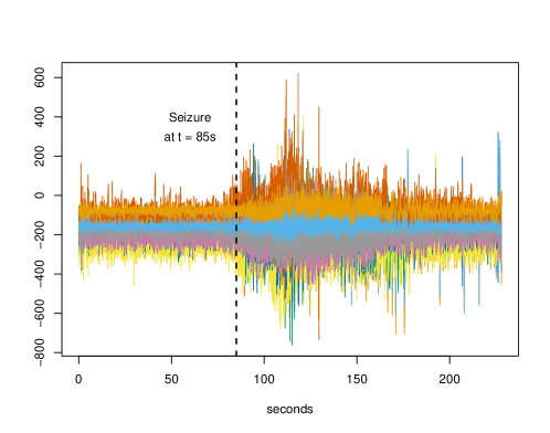
Figure 1: EEG signals from a patient diagnosed with left temporal lobe epilepsy. The data was recorded at 18 locations on the scalp during an epileptic seizure over 228 seconds.

By modeling the two time series (before and after the seizure) using the VAR model in (1), this problem amounts to detecting differences between the transition matrices of the two VAR models, which is an example of differential network analysis (Shojaie, 2021). Consider two stationary $d$-dimensional time series that satisfy

$${\bf x}^{(l)}_{t}=\sum_{k=1}^{p}A_{k}^{(l)^{\intercal}}{\bf x}^{(l)}_{t-k}+{{\mbox{\boldmath${\epsilon}$}}}_{t}^{(l)},~{}\mbox{~{}}t=p+1,\ldots,n_{l},$$ (2)

where ${{\mbox{\boldmath${\epsilon}$}}}_{t}^{(l)}{\sim}N(0,\Psi_{l})$ and $E[{\mbox{\boldmath${\epsilon}$}}_{t}^{(l)}{\mbox{\boldmath${\epsilon}$}}_{t+i}^{(l)}]={\bf 0}$ for all $t,i\in\mathbb{N}$ and $l=1,2$. We aim to estimate $\Delta_{A,k}=A^{(1)}_{k}-A^{(2)}_{k}$ for $k=1,\ldots,p$, which collectively characterize the changes in Granger causal relations between the two VAR models, called differential Granger causality hereafter. Letting

$$\widetilde{\bf x}^{(l)}_{t}=\left(\begin{array}[]{c}{\bf x}^{(l)}_{t+p-1}\\ {\bf x}^{(l)}_{t+p-2}\\ \vdots\\ {\bf x}^{(l)}_{t}\end{array}\right),\quad\widetilde{A}^{(l)}=\left(\begin{array}[]{ccccc}A_{1}^{(l)}&I_{d}&0&\dots&0\\ \vdots&\ddots&\ddots&\ddots&\vdots\\ A_{p-1}^{(l)}&0&0&\dots&I_{d}\\ A_{p}^{(l)}&0&0&\dots&0\end{array}\right),\quad\widetilde{{\mbox{\boldmath${\epsilon}$}}}^{(l)}_{t}=\left(\begin{array}[]{c}{{\mbox{\boldmath${\epsilon}$}}}^{(l)}_{t+p-1}\\ 0\\ \vdots\\ 0\end{array}\right),$$

we can reformulate the VAR($p$) model in (2) as the following VAR(1) model

$$\widetilde{\bf x}^{(l)}_{t}=\widetilde{A}^{(l)^{\intercal}}\widetilde{\bf x}^{(l)}_{t-1}+\widetilde{{\mbox{\boldmath${\epsilon}$}}}_{t}^{(l)},~{}t=1,\ldots,n_{l}-p+1.$$ (3)

In the following discussions, without loss of generality, we shall focus on this reformulated VAR(1) model and aim to estimate $\Delta_{A}=\widetilde{A}^{(1)}-\widetilde{A}^{(2)}$.

To the best of our knowledge, the only existing way to estimate $\Delta_{A}$ is to first separately estimate $\widetilde{A}^{(1)}$ and $\widetilde{A}^{(2)}$ using the aforementioned penalized methods and then find the difference. We call this approach separate estimation hereafter. In high-dimensional settings, consistency of any separate estimation approach based on the $l_{1}$-penalty requires the sparsity of each ${A}_{k}^{(l)}$ for $k=1,\ldots,p$ and $l=1,2$. However, this sparsity assumption may be violated in real applications. For example, many studies have demonstrated the existence and importance of hub nodes in human brain networks (Buckner et al., 2009). These hub nodes interact with many brain regions and distribute information in powerful ways (Power et al., 2013). As a result, the rows and/or columns of the transition matrix corresponding to these hub nodes may have many nonzero entries, leading to the violation of the sparsity assumption.

To alleviate this issue, we propose a novel approach to directly estimate $\Delta_{A}$, without requiring sparsity of individual transition matrices. Key to our approach is a new estimating equation for $\Delta_{A}$ based on the Yule-Walker equation (Lütkepohl, 2005) for the VAR models (3). This estimating equation links $\Delta_{A}$ with $\Delta_{\Omega}=\Sigma_{1}^{-1}-\Sigma_{2}^{-1}$, where $\Sigma_{l}=\mbox{cov}\left(\widetilde{{\bf x}}_{t}^{(l)}\right)$ for $l=1,2$. Here, $\Sigma_{l}$ is constant across all time points because both time series are assumed to be stationary. Based on the estimating equation, we estimate $\Delta_{A}$ in two steps. First, we directly estimate $\Delta_{\Omega}$ via the lasso penalized D-trace regression (Zhang and Zou, 2014), which is a special case of the score matching estimator (Lin et al., 2016; Yu et al., 2019). The same approach was adopted in Yuan et al. (2017) to estimate $\Delta_{\Omega}$ when data are i.i.d under each condition. Zhao et al. (2014) proposed an alternative but more computationally intensive approach for direct estimation of differences in precision matrices with i.i.d data via the constrained $l_{1}$ minimization (Cai et al., 2011). We adopt the the D-trace approach due to its computational advantages. Both Yuan et al. (2017) and Zhao et al. (2014) establish consistency results for their estimators of $\Delta_{\Omega}$ under various conditions. However, the key assumptions, i.e., the mutual incoherence (MI) condition in Zhao et al. (2014) and the irrepresentability (IR) condition in Yuan et al. (2017), are stringent. Indeed, we show in Section 3.3 that these two conditions rarely hold, especially for large $d$. To address this issue, we establish novel consistency results for the D-trace estimator of $\Delta_{\Omega}$ under weaker conditions. Specifically, for estimation of $\Delta_{\Omega}$ with i.i.d data, we only require the sparsity of $\Delta_{\Omega}$; notably, the established convergence rate is also potentially faster than that shown in Yuan et al. (2017). We also establish similar consistency results for the time series in (3) under an additional spectral density assumption. Second, using the Yule-Walker estimating equation that links $\Delta_{A}$ and $\Delta_{\Omega}$, we construct a lasso penalized quadratic loss function to estimate $\Delta_{A}$. Computationally, this optimization problem can be decomposed into $d$ independent ones and is fast to solve via parallel computation. Theoretically, assuming the sparsity of the columns of $\Delta_{A}$, we prove element-wise, Frobenius-norm, and variable-selection consistency of our direct estimator of $\Delta_{A}$. Extensive numerical studies corroborate these results.

1.3 Notation

We denote scalars, vectors, and matrices using lowercase, bold lowercase, and uppercase letters, respectively. Let $I(\mathcal{A})$ be the indicator of event $\mathcal{A}$; i.e., $I(\mathcal{A})=1$ if $\mathcal{A}$ is true, and $I(\mathcal{A})=0$ otherwise. For a $d$-dimensional vector ${\bf v}=\left(v_{1},\dots,v_{d}\right)^{\intercal}$, we define the following vector norms

$$\|{\bf v}\|_{0}=\sum_{j=1}^{d}I\left(v_{j}\neq 0\right),\quad\|{\bf v}\|_{q}=\Bigg{(}\sum_{j=1}^{d}\left|v_{j}\right|^{q}\Bigg{)}^{1/q},\quad\|{\bf v}\|_{\infty}=\max_{1\leq j\leq d}\left|v_{j}\right|.$$

For a $d\times d$ matrix $M=\left(m_{jk}\right)_{j,k=1,\ldots,d}$, we write $\mbox{vec}(M)$ for the $d^{2}$-dimensional vector by stacking the columns of $M$. We define

$$\|M\|_{\max}=\max_{jk}\left|m_{jk}\right|~{},~{}\|M\|_{\mathrm{F}}=\Bigg{(}\sum_{j,k}\left|m_{jk}\right|^{2}\Bigg{)}^{1/2},~{}\|M\|_{q}=\max_{\|v\|_{q}=1}\|Mv\|_{q}$$

for $0<q\leq\infty$. We also define $|M|_{1}=\sum_{jk}|m_{jk}|$, $|M|_{0}=\sum_{jk}I\left(m_{jk}\neq 0\right)$, and let $\lambda_{\min}(M)$ and $\lambda_{\max}(M)$ denote the smallest and largest eigenvalue of $M$, respectively. For arbitrary matrices $A$ and $B$, we denote by $A\otimes B$ the Kronecker product of $A$ and $B$, and define $\left\langle A,B\right\rangle=\mbox{tr}(AB^{\intercal})$ if $A$ and $B$ have compatible dimensions.

2 Method

Our direct estimation procedure leverages the connection between $\Delta_{A}$ and $\Delta_{\Omega}$. By the Yule-Walker equation (Lütkepohl, 2005) for model (3), we have $\widetilde{A}^{(l)}=\Sigma_{l}^{-1}\Theta_{l},$ where $\Theta_{l}=E\left(\widetilde{\bf x}^{(l)}_{t}\widetilde{\bf x}^{(l)^{\intercal}}_{t+1}\right)$ is the lag-1 auto-covariance matrix of $\widetilde{\bf x}^{(l)}_{t}$ for $l=1,2$. Thus,

$$\Delta_{A} ~{}=\widetilde{A}^{(1)}-\widetilde{A}^{(2)}=\Sigma_{1}^{-1}\Theta_{1}-\Sigma_{2}^{-1}\Theta_{2}$$

$$~{}=\Delta_{\Omega}\Theta_{1}+\Sigma_{2}^{-1}(\Theta_{1}-\Theta_{2})$$

$$~{}=\Delta_{\Omega}\Theta_{2}+\Sigma_{1}^{-1}(\Theta_{1}-\Theta_{2})$$

and $\Delta_{A}$ satisfies the following estimating equation, which is the basis of our direct estimation approach,

$$(\Sigma_{1}+\Sigma_{2})\Delta_{A}=\Sigma_{1}\Delta_{\Omega}\Theta_{2}+\Sigma_{2}\Delta_{\Omega}\Theta_{1}+2(\Theta_{1}-\Theta_{2}).$$ (4)

In practice, we need to replace the population-level quantities in (4) with their estimates. Natural estimates of $\Sigma_{l}$ and $\Theta_{l}$ are, respectively, given by

$$\widehat{\Sigma}_{l}=\frac{1}{n_{l}-p+1}\sum_{t=1}^{{n_{l}-p+1}}\widetilde{\bf x}_{t}\widetilde{\bf x}_{t}^{\intercal},~{}~{}\widehat{\Theta}_{l}=\frac{1}{n_{l}-p}\sum_{t=1}^{n_{l}-p}\widetilde{\bf x}_{t}\widetilde{\bf x}_{t+1}^{\intercal}~{}\mbox{for}~{}l=1,2.$$ (5)

Subsequently, a natural estimator of $\Delta_{\Omega}$ is $\widehat{\Sigma}_{1}^{-1}-\widehat{\Sigma}_{2}^{-1}$ if each $\widehat{\Sigma}_{l}$ is non-singular. However, this estimator of $\Delta_{\Omega}$ is ill-posed in high-dimensional settings. When each $\Sigma_{l}^{-1}$ is sparse, $l_{1}$-penalization approaches, including the graphical lasso (Friedman et al., 2008), neighborhood selection (Meinshausen et al., 2006), and $l_{1}$-constrained minimization (Cai et al., 2011; Han et al., 2015), give consistent estimates of $\Sigma_{l}^{-1}$. However, each $\Sigma_{l}^{-1}$ is likely not sparse when hub nodes exist in the $l$-th time series. Specifically, under Gaussianity, zero entries in an inverse covariance matrix characterize conditional independence between variables. Thus, if hub nodes exist, then the rows and columns of the inverse covariance matrix corresponding to the hub nodes would have many nonzero entries, leading to a non-sparse inverse convariance matrix.

To overcome the above limitations, we directly estimate $\Delta_{\Omega}$ using the lasso penalized D-trace approach, which does not require $\Sigma_{l}^{-1}$ to be sparse. We define the following D-trace loss function

$$L_{\mathrm{D}}\left(\Delta_{\Omega},\Sigma_{1},\Sigma_{2}\right)=\frac{1}{4}\large(\left\langle\Sigma_{1}\Delta_{\Omega},\Delta_{\Omega}\Sigma_{2}\right\rangle+\left\langle\Sigma_{2}\Delta_{\Omega},\Delta_{\Omega}\Sigma_{1}\right\rangle\large)-\left\langle\Delta_{\Omega},\Sigma_{1}-\Sigma_{2}\right\rangle.$$ (6)

Then,

$$\frac{\partial L_{\mathrm{D}}\left(\Delta_{\Omega},\Sigma_{1},\Sigma_{2}\right)}{\partial\Delta_{\Omega}} =\frac{1}{2}(\Sigma_{1}\Delta_{\Omega}\Sigma_{2}+\Sigma_{2}\Delta_{\Omega}\Sigma_{1})-(\Sigma_{1}-\Sigma_{2})=0,$$ (7)

$$\frac{\partial^{2}L_{D}(\Delta_{\Omega},\Sigma_{1},\Sigma_{2})}{\partial\Delta_{\Omega}\partial\Delta_{\Omega}^{\intercal}} =\frac{1}{2}(\Sigma_{1}\otimes\Sigma_{2}+\Sigma_{2}\otimes\Sigma_{1})\succ 0,$$ (8)

where $M\succ 0$ means that matrix $M$ is positive definite. Thus, the D-trace loss function in (6) has a unique minimizer at $\Delta_{\Omega}$. By replacing $\Sigma_{l}$ by $\widehat{\Sigma}_{l}$ for $l=1,2$, we estimate $\Delta_{\Omega}$ as

$$\widehat{\Delta}_{\Omega}(\nu)=\operatorname*{argmin}_{\Delta_{\Omega}}\left\{L_{\mathrm{D}}\left(\Delta_{\Omega},\widehat{\Sigma}_{1},\widehat{\Sigma}_{2}\right)+\nu|\Delta_{\Omega}|_{1}\right\},$$ (9)

where $\nu>0$ is a tuning parameter. An efficient algorithm for optimizing (9) was proposed in Yuan et al. (2017).

Remark 1.

Zhao et al. (2014) proposed an alternative approach for estimating $\Delta_{\Omega}$ via the $l_{1}$-constrained minimization (Cai et al., 2011), when data are i.i.d within each group. However, this approach is computationally less efficient than the approach based on the D-trace loss, especially for large $d$. As discussed in Yuan et al. (2017), the computational complexity and the memory requirement of the $l_{1}$-constrained minimization approach both scale as $O(d^{4})$, whereas the D-trace loss approach requires $O(d^{3})$ computational complexity and $O(d^{2})$ memory.

Given $\widehat{\Sigma}_{l}$ and $\widehat{\Theta}_{l}$ in (5) and $\widehat{\Delta}_{\Omega}(\nu)$ in (9), we next estimate $\Delta_{A}$ based on the estimating equation (4). This optimization problem can be further decomposed into $d$ parallel equations, each corresponding to one column of $\Delta_{A}$. More specifically, let ${\mbox{\boldmath${\beta}$}}_{j}$ and ${\bf w}_{j}$, respectively, denote the $j$-th column of $\Delta_{A}$ and $\Sigma_{1}\Delta_{\Omega}\Theta_{2}+\Sigma_{2}\Delta_{\Omega}\Theta_{1}+2(\Theta_{1}-\Theta_{2})$. Then, (4) amounts to

$$(\Sigma_{1}+\Sigma_{2}){\mbox{\boldmath${\beta}$}}_{j}-{\bf w}_{j}=0~{}\mbox{for~{}}j=1,\ldots,d.$$ (10)

This leads to the following quadratic loss function that has a unique minimizer at ${\mbox{\boldmath${\beta}$}}_{j}$:

$$L_{A}\left({\mbox{\boldmath${\beta}$}}_{j};\Sigma_{1},\Sigma_{2},\Delta_{\Omega},\Theta_{1},\Theta_{2}\right)=\frac{1}{2}{\mbox{\boldmath${\beta}$}}_{j}^{\intercal}\left(\Sigma_{1}+\Sigma_{2}\right){\mbox{\boldmath${\beta}$}}_{j}-{\mbox{\boldmath${\beta}$}}_{j}^{T}{\bf w}_{j}.$$

Thus, we propose to estimate ${\mbox{\boldmath${\beta}$}}_{j}$ as

$$\widehat{{\mbox{\boldmath${\beta}$}}}_{j}(\lambda_{j})=\operatorname*{argmin}_{{\mbox{\boldmath${\beta}$}}_{j}}\left\{L_{A}\left({\mbox{\boldmath${\beta}$}}_{j};\widehat{\Sigma}_{1},\widehat{\Sigma}_{2},\widehat{\Delta}_{\Omega},\widehat{\Theta}_{1},\widehat{\Theta}_{2}\right)+\lambda_{j}\|{\mbox{\boldmath${\beta}$}}_{j}\|_{1}\right\},$$ (11)

where $\lambda_{j}>0$ is a tuning parameter. For $j=1,\ldots,d$, we solve (11) using the coordinate descent algorithm (Wright, 2015) in parallel. Finally, our direct estimator of $\Delta_{A}$ is the matrix with the $j$-th column being $\widehat{{\mbox{\boldmath${\beta}$}}}_{j}(\lambda_{j})$, denoted by

$$\widehat{\Delta}_{A}({\mbox{\boldmath${\lambda}$}})=\left[\widehat{{\mbox{\boldmath${\beta}$}}}_{1}(\lambda_{1})\cdots\widehat{{\mbox{\boldmath${\beta}$}}}_{d}(\lambda_{d})\right].$$

The numerical performance of $\widehat{\Delta}_{A}({\mbox{\boldmath${\lambda}$}})$ and $\widehat{\Delta}_{\Omega}(\nu)$ depends on the choice of the tuning parameters. We select the tuning parameters using an approximate Bayesian information criterion (aBIC), similar to the criterion in Zhao et al. (2014). Specifically, letting $a_{n_{1},n_{2},p}=n_{1}+n_{2}-2(p-1)$, the optimal $\nu_{\text{opt}}$ is chosen to minimize

$$a_{n_{1},n_{2},p}\left\|\frac{1}{2}\left(\widehat{\Sigma}_{1}\widehat{\Delta}_{\Omega}(\nu)\widehat{\Sigma}_{2}+\widehat{\Sigma}_{2}\widehat{\Delta}_{\Omega}(\nu)\widehat{\Sigma}_{1}\right)-(\widehat{\Sigma}_{1}-\widehat{\Sigma}_{2})\right\|_{\max}+\log\left(a_{n_{1},n_{2},p}\right)\left|\widehat{\Delta}_{\Omega}(\nu)\right|_{0}.$$

With $\nu_{\text{opt}}$, each $\lambda_{j}$ is determined by minimizing

$$a_{n_{1},n_{2},p}\left\|\left(\widehat{\Sigma}_{1}+\widehat{\Sigma}_{2}\right)\widehat{{\mbox{\boldmath${\beta}$}}}_{j}(\lambda_{j})-\widehat{\bf w}_{j}\right\|_{\max}+\log\left(a_{n_{1},n_{2},p}\right)\left\|\widehat{{\mbox{\boldmath${\beta}$}}}_{j}\right\|_{0},$$

where $\widehat{\bf w}_{j}$ is the $j$-th column of $\widehat{\Sigma}_{1}\widehat{\Delta}_{\Omega}(\nu_{\text{opt}})\widehat{\Theta}_{2}+\widehat{\Sigma}_{2}\widehat{\Delta}_{\Omega}(\nu_{\text{opt}})\widehat{\Theta}_{1}+2(\widehat{\Theta}_{1}-\widehat{\Theta}_{2})$.

3 Theoretical Properties

3.1 Convergence Rates of $\widehat{\Delta}_{\Omega}(\nu)$

In this subsection, we establish nonasymptotic convergence rates for $\widehat{\Delta}_{\Omega}(\nu)$ under model (3). We first introduce some additional notations. Let $S_{\Omega}$ denote the indices of the nonzero entries in $\Delta_{\Omega}$; that is, $S_{\Omega}=\{(j,k)\mathrel{\mathop{\mathchar 58\relax}}(\Delta_{\Omega})_{jk}\neq 0\}$. Also, denote by $s_{\Omega}$ the number of nonzero entries in $\Delta_{\Omega}$, i.e., $s_{\Omega}=|\Delta_{\Omega}|_{0}$. For an arbitrary stationary stochastic process $\{{\bf z}_{t}\}_{t\in\mathbb{N}}$, we define $\Gamma(h)=\mbox{cov}({\bf z}_{t},{\bf z}_{t+h})$ for all $t,h\in\mathbb{N}$ as the lag-$h$ auto-covariance matrix of ${\bf z}_{t}$. The following condition controls the stability of $\{{\bf z}_{t}\}_{t\in\mathbb{N}}$ in terms of its spectral density.

Assumption 1.

The spectral density function

$$f(\theta)=\frac{1}{2\pi}\sum_{h=-\infty}^{\infty}\Gamma(h)e^{-ih\theta},~{}\theta\in[-\pi,\pi]$$

exists, and its maximum eigenvalue is bounded almost everywhere on $[-\pi,\pi]$; that is,

$$\mathcal{M}(f)=\mbox{ess sup}_{\theta\in[-\pi,\pi]}\lambda_{\max}(f(\theta))<\infty.$$

The spectral density is the analogue of the probability density function. Processes with larger $\mathcal{M}(f)$ are considered less stable. As discussed in Douc et al. (2014), a large class of linear processes, including stable and invertible ARMA processes, satisfy Assumption 1. An alternative assumption for controlling the stability is that the eigenvalues of the transition matrix of the VAR model have modulus less than 1 (Loh and Wainwright, 2012; Han et al., 2015), referred to as the modulus assumption hereafter. We adopt the spectral density assumption rather than the modulus assumption for two reasons. First, the modulus assumption constraints each transition matrix. However, since we aim to directly estimate the difference of two transition matrices, constraints on individual transition matrices are not desirable. Second, the spectral density assumption is less restrictive than the modulus assumption. This can be seen for a VAR(1) model with transition matrix $A$, where the modulus assumption reduces to $\|A\|_{2}=c$ for some constant $c<1$. On the one hand, $\|\Gamma(h)\|_{2}\leq c^{|h|}\|\Gamma(0)\|_{2}$. This indicates that the spectral density function $f(\theta)$ exists, and $\mathcal{M}(f)\leq(1-c)^{-1}\pi^{-1}\|\Gamma(0)\|_{2}<\infty$. On the other hand, one can construct examples where Assumption 1 is satisfied but $\|A\|_{2}>1$; see Examples 1 and 2 in Basu and Michailidis (2015).

The following theorem establishes convergence rates for the lasso penalized D-trace estimator $\widehat{\Delta}_{\Omega}(\nu)$ in terms of the Frobenius and element-wise norms.

Theorem 1.

Suppose that ${\bf x}_{t}^{(l)}$ satisfies Assumption 1 with the spectral density $f_{l}(\cdot)$ for $l=1,2$. Denote $C_{M}=\max\left(\mathcal{M}(f_{1}),\mathcal{M}(f_{2})\right)$ and $C_{\Sigma}=\max\left(\|\Sigma_{1}\|_{\max},\|\Sigma_{2}\|_{\max}\right)$. Consider

$$\nu=128\sqrt{6}\pi C_{M}(1+C_{\Sigma}\|\Delta_{\Omega}\|_{1})\left(\frac{\log d}{\min(n_{1},n_{2})-(p-1)}\right)^{1/2}.$$

If $d>1$, $\min(n_{1},n_{2})\geq C_{G}s_{\Omega}^{2}\log d+p-1$ with $C_{G}$ given in equation (28) in the appendix, then with probability at least $1-16d^{-1}$, we have

$$\left\|\widehat{\Delta}_{\Omega}(\nu)-\Delta_{\Omega}\right\|_{F}~{} \leq 6s_{\Omega}^{1/2}\lambda_{\min}^{-1}(\Sigma_{1})\lambda_{\min}^{-1}(\Sigma_{2})\nu,$$ (12)

$$\left\|\widehat{\Delta}_{\Omega}(\nu)-\Delta_{\Omega}\right\|_{\max}~{} \leq 6s_{\Omega}^{1/2}\lambda_{\min}^{-1}(\Sigma_{1})\lambda_{\min}^{-1}(\Sigma_{2})\nu.$$ (13)

To prove Theorem 1, we adopt the general framework of Negahban et al. (2012) for theoretical analysis of a broad class of penalized M-estimators with norm-based decomposable regularizers, including our D-trace estimator $\widehat{\Delta}_{\Omega}(\nu)$; see Lemma 8 in the appendix for more details.

Theorem 1 indicates that $\widehat{\Delta}_{\Omega}(\nu)$ can include all nonzero entries in $\Delta_{\Omega}$ that are “large enough" but may not exclude all zeros. In the following, we provide a refinement of Theorem 1 that can lead to consistent variable selection. More specifically, for $\tau>0$, we define the hard thresholding function $\mbox{HT}_{\tau}(t)=tI(|t|>\tau)$, and let $\mbox{sgn}(t)$ denote the sign function. For any matrix $M$, denote $\mbox{HT}_{\tau}(M)=\left(\mbox{HT}_{\tau}(M_{jk})\right)_{jk}$ and $\mbox{sgn}(M)=\left(\mbox{sgn}(M_{jk})\right)_{jk}$. The following result characterizes the sign consistency of $\mbox{HT}_{\tau_{\Omega}}\left(\widehat{\Delta}_{\Omega}(\nu)\right)$ for an appropriately chosen $\tau_{\Omega}$, when the non-zero entries in $\Delta_{\Omega}$ are sufficiently large.

Theorem 2.

Suppose that ${\bf x}_{t}^{(l)}$ satisfies Assumption 1 with the spectral density $f_{l}(\cdot)$ for $l=1,2$. For $n_{1},n_{2},d$ and $\nu$ that satisfy the same conditions as in Theorem 1, if

$$\tau_{\Omega}\geq 6s_{\Omega}^{1/2}\lambda_{\min}^{-1}(\Sigma_{1})\lambda_{\min}^{-1}(\Sigma_{2})\nu$$

and $\min_{(j,k)\mathrel{\mathop{\mathchar 58\relax}}(\Delta_{\Omega})_{jk}\neq 0}\left|(\Delta_{\Omega})_{jk}\right|>2\tau_{\Omega}$, then with probability at least $1-16d^{-1}$, $\mbox{sgn}\left(\mbox{HT}_{\tau_{\Omega}}\left(\widehat{\Delta}_{\Omega}(\nu)\right)\right)=\mbox{sgn}(\Delta_{\Omega})$.

3.2 Convergence Rates of $\widehat{\Delta}_{A}({\mbox{\boldmath${\lambda}$}})$

Based on Theorem 1, we establish convergence rates for $\widehat{\Delta}_{A}({\mbox{\boldmath${\lambda}$}})$ in terms of the Frobenius and element-wise norms. For $j=1,\ldots,d$, recalling that ${\mbox{\boldmath${\beta}$}}_{j}$ denotes the $j$-th column of $\Delta_{A}$, we denote the active set of ${\mbox{\boldmath${\beta}$}}_{j}$ by $S_{A,j}$ and $s_{A,j}=\|{\mbox{\boldmath${\beta}$}}_{j}\|_{0}$. Also, let

$$C_{1}=64\sqrt{6}\pi C_{M}(1+\|\Delta_{A}\|_{1})+C_{I_{12}}|\Delta_{\Omega}|_{1}+\left\{s_{\Omega}(1+C_{\Sigma}|\Delta_{\Omega}|_{1})\lambda_{\min}^{-1}(\Sigma_{1})\lambda_{\min}^{-1}(\Sigma_{2})+1/96\right\}C_{I_{3}},$$

where $C_{I_{12}}$ and $C_{I_{3}}$ are given in eq. (A.13) in the appendix.

Theorem 3.

Suppose that ${\bf x}_{t}^{(l)}$ satisfies Assumption 1 with the spectral density $f_{l}(\cdot)$ for $l=1,2$. Consider the same $\nu$ as in Theorem 1 and

$$\lambda_{j}=2C_{1}\left(\frac{\log d}{\min(n_{1},n_{2})-p}\right)^{1/2},~{}j=1,\ldots,d.$$

If $d>1$ and $n_{1}$ and $n_{2}$ are sufficiently large, then with probability at least $1-32d^{-1}$, we have

$$\left\|\widehat{\Delta}_{A}({\mbox{\boldmath${\lambda}$}})-\Delta_{A}\right\|_{F}~{} \leq 6\lambda_{j}\left\{\lambda_{\min}(\Sigma_{1})+\lambda_{\min}(\Sigma_{2})\right\}^{-1}\left(\sum_{j=1}^{d}s_{A,j}^{2}\right)^{1/2},$$ (14)

$$\left\|\widehat{\Delta}_{A}({\mbox{\boldmath${\lambda}$}})-\Delta_{A}\right\|_{\max}~{} \leq 6\lambda_{j}\left\{\lambda_{\min}(\Sigma_{1})+\lambda_{\min}(\Sigma_{2})\right\}^{-1}\max_{j}s_{A,j}.$$ (15)

The specific conditions for $n_{1}$ and $n_{2}$ are given in equations (7.1) and (32) in the appendix. The techniques for proving Theorem 3 are similar to those for proving Theorem 1. However, unlike Theorem 1 where the convergence rates are the same for the Frobenius and element-wise norms, the convergence rate of the element-wise norm error in (15) is potentially faster than that of the Frobenius norm error in (14). This is due to the parallel computation of $\widehat{\Delta}_{A}({\mbox{\boldmath${\lambda}$}})$; see the proof of Theorem 3 in the appendix for the details.

Similar to Theorem 2, the next result establishes variable selection consistency of $\mbox{HT}_{\tau_{A}}\left(\widehat{\Delta}_{A}({\mbox{\boldmath${\lambda}$}})\right)$ for an suitable $\tau_{A}$, when the non-zero entries in $\Delta_{A}$ are sufficiently large.

Theorem 4.

Suppose ${\bf x}_{t}^{(l)}$ satisfies Assumption 1 with the spectral density $f_{l}(\cdot)$ for $l=1,2$. For $n_{1},n_{2},d$ and $\{\lambda_{j}\}_{j=1,\ldots,d}$ that satisfy the same conditions as in Theorem 3, if

$$\tau_{A}\geq ~{}6\lambda_{j}\left\{\lambda_{\min}(\Sigma_{1})+\lambda_{\min}(\Sigma_{2})\right\}^{-1}\max_{j}s_{A,j},$$

and $\min_{(j,k)\mathrel{\mathop{\mathchar 58\relax}}(\Delta_{A})_{jk}\neq 0}|(\Delta_{A})_{jk}|>2\tau_{A}$, then with probability at least $1-32d^{-1}$, $\mbox{sgn}\left(\mbox{HT}_{\tau_{A}}\left(\widehat{\Delta}_{A}({\mbox{\boldmath${\lambda}$}})\right)\right)=\mbox{sgn}(\Delta_{A})$.

3.3 Comparison of Assumptions and Rates of Convergence

When the data within each group are i.i.d, Theorem 1 requires less stringent assumptions than those in existing theoretical results, namely, the mutual incoherence (MI) condition in Zhao et al. (2014), and the irrepresentability (IR) condition in Yuan et al. (2017). Both conditions are related to the sparsity $s_{\Omega}$, dimension $d$, and maximum correlation in $\Sigma_{l}$ for $l=1,2$, and can be restrictive in practice, especially for large $d$ and highly correlated variables.

We first show that the MI condition seldom holds if some variables have strong correlations. Let $\sigma_{l,jk}$ be the $(j,k)$-th entry of $\Sigma_{l}$, and denote $\sigma_{l,\max}=\max_{j}\sigma_{l,jj}$, $\sigma_{l,\min}=\min_{j}\sigma_{l,jj}$ and $\mu_{l}=\max_{j\neq k}|\sigma_{l,jk}|$ for $l=1,2$. Then, the MI condition is

$$\mu=4\max(\mu_{1}\sigma_{2,\max},\mu_{2}\sigma_{1,\max})\leq\sigma^{S}_{\min}(2s_{\Omega}^{\prime})^{-1},$$ (16)

where $\sigma^{S}_{\min}=\min_{j,k}(\sigma_{2,jj}\sigma_{1,jj},\sigma_{2,kk}\sigma_{1,jj}+2\sigma_{2,kj}\sigma_{1,jk}+\sigma_{2,jj}\sigma_{1,kk})$, and $s_{\Omega}^{\prime}$ is the number of nonzero entries in the upper triangular part of the true $\Delta_{\Omega}$. To gain more intuition about this condition, we consider a special example where all the variables have been standardized; that is, $\sigma_{l,jj}=1$ for $l=1,2$ and $j=1,\ldots,d$. In this case, $\sigma_{\min}^{S}\leq 1$, and (16) reduces to $\max(\mu_{1},\mu_{2})\leq(8s_{\Omega}^{\prime})^{-1}$. This implies that the maximum correlation among the variables cannot exceed $1/8$ because $s_{\Omega}^{\prime}\geq 1$; the case of $s_{\Omega}^{\prime}=0$ is trivial. However, this constraint on between-variable correlations is unrealistic in many applications.

The IR condition in Yuan et al. (2017) requires that

$$\max_{e\in S_{\Omega}^{c}}\left\|\Gamma_{e,S_{\Omega}}(\Gamma_{S_{\Omega},S_{\Omega}})^{-1}\right\|_{1}<1,$$ (17)

where $\Gamma$ denotes the Hessian matrix in (8), and $S_{\Omega}$ is the support of $\Delta_{\Omega}$. We examine how often (17) is satisfied using a simulation study. Specifically, we generated $\Sigma_{1}^{-1}\in\mathbb{R}^{d\times d}$ from Erdös-Rënyi graphs with $d$ nodes and $d(d-1)/5$ nonzero off-diagonal entries for $d=10,20,30,40,$ and 50. The values in the off-diagonal nonzero entries were generated from a uniform distribution with support $[-1,-0.5]\bigcup[0.5,1]$, and the diagonal entries were set to be $10$. Then, $\Sigma_{2}^{-1}$ was generated by changing the sign of $s_{\Omega}$ nonzero entries of $\Sigma_{1}^{-1}$. Let $S_{\Omega}$ denote the indices of the $s_{\Omega}$ entries, that is, $S_{\Omega}=\{(j,k)\mathrel{\mathop{\mathchar 58\relax}}(\Sigma_{2}^{-1})_{jk}\neq(\Sigma_{1}^{-1})_{jk}\}$. The matrices $\Sigma_{1}$ and $\Sigma_{2}$ were obtained by inverting $\Sigma_{1}^{-1}$ and $\Sigma_{2}^{-1}$, respectively. The maximum correlation in the covariance matrix $\Sigma_{l}$ is around $0.1$ for $l=1,2$, which represents a setting with weakly correlated variables. We then calculated $\Gamma=0.5(\Sigma_{1}\otimes\Sigma_{2}+\Sigma_{2}\otimes\Sigma_{1})$ and examined (17). Table 1 shows how often (17) holds with various $d$ and $s_{\Omega}$. For small $d$, e.g., $d=10$, (17) holds with high probability. However, as $d$ grows, the percentage of cases where (17) holds drops quickly. Particularly, when $d\geq 30$, even for the very sparse case $s_{\Omega}=6$, (17) never holds. These results indicate that the IR condition in (17) is not realistic even with moderate $d$, small $s_{\Omega}$, and weakly correlated variables.

Table 1: Percentages of simulated $\Gamma$ in $1000$ simulations that meet the IR condition (%)

$d$	10	20	30	40	50
$s_{\Omega}=6$	100	12.9	0	0	0
$s_{\Omega}=12$	100	4.9	0	0	0
$s_{\Omega}=18$	100	3.1	0	0	0

Theorem 1 relaxes these stringent conditions because when data in each group are i.i.d, our Condition 1 becomes trivial. Despite requiring less restrictive conditions, our convergence rate in Theorem 1 may be faster than that Yuan et al. (2017). Take the bound of $\|\widehat{\Delta}_{\Omega}(\nu)-\Delta_{\Omega}\|_{\max}$ as an example. Yuan et al. (2017) show that for a suitable $\nu$, $\|\widehat{\Delta}_{\Omega}(\nu)-\Delta_{\Omega}\|_{\max}\leq M_{Y}(\eta\log d+\log 4)^{1/2}\{\min(n_{1},n_{2})\}^{-1/2}$ for some constants $M_{Y}>0$ and $\eta>2$. By carefully examining their proof, particularly, equations (A6) and (A7), we find that $M_{Y}=O(s_{\Omega}^{3})$. In comparison, Theorem 1 shows that $\|\widehat{\Delta}_{\Omega}(\nu)-\Delta_{\Omega}\|_{\max}\leq M_{W}(\log d)^{1/2}\{\min(n_{1},n_{2})\}^{-1/2}$, where $M_{W}=O\left(|\Delta_{\Omega}|_{1}s_{\Omega}^{1/2}\lambda_{\min}^{-1}(\Sigma_{1})\lambda_{\min}^{-1}(\Sigma_{2})\right)$ and $|\Delta_{\Omega}|_{1}\leq s_{\Omega}\|\Delta_{\Omega}\|_{\max}$. Hence, if $\|\Delta_{\Omega}\|_{\max}=O(1)$ and $\lambda_{\min}^{-1}(\Sigma_{1})\lambda_{\min}^{-1}(\Sigma_{2})=o(s_{\Omega}^{3/2})$, then $M_{W}=o(s_{\Omega}^{3})$, indicating that our convergence rate is potentially faster than that in Yuan et al. (2017).

4 Simulations

4.1 Simulation I

In this simulation, we evaluate the finite sample performance of the proposed direct estimator $\widehat{\Delta}_{A}({\mbox{\boldmath${\lambda}$}})$ in identifying the nonzero entries of $\Delta_{A}$ under a VAR(1) model. To this end, we simulated $\Sigma_{1}^{-1}$ and $\Sigma_{2}^{-1}$ similar to Zhao et al. (2014). Specifically, the support of $\Sigma_{1}^{-1}$ was simulated according to a network with $d=20,50,100$ nodes and $60\%$ nonzero entries. The value of each nonzero entry of $\Sigma_{1}^{-1}$ was then generated from a uniform distribution with support $[-0.5,-0.2]\bigcup[0.2,0.5]$. We scaled each row of $\Sigma_{1}^{-1}$ by $3,4$ and $5$ for $d=20,50$ and $100$, respectively, to ensure its positive definiteness. Then, the diagonals of $\Sigma_{1}^{-1}$ were set to 1 and the matrix was symmetrized by averaging it with its transpose. The matrix $\Sigma_{2}^{-1}$ was generated such that the largest $0.4d$ (by magnitude) of $\Sigma_{1}^{-1}$ entries changed sign between $\Sigma_{1}^{-1}$ and $\Sigma_{2}^{-1}$. As such, $\Sigma_{2}^{-1}$ is still guaranteed positive definite. We took a similar approach to generate $A^{(1)}$ and $A^{(2)}$. The support of $A^{(1)}$ was generated according to a directed network with $d=20,50,100$ nodes with $70\%$ nonzero entries. The value of each nonzero entry was then generated from a uniform distribution with support $[-0.8,-0.5]\bigcup[0.5,0.8]$. We scaled $A^{(1)}$ such that $\|A^{(1)}\|_{2}=0.6$. The difference $\Delta_{A}=A^{(1)}-A^{(2)}$ was generated such that the largest $0.5d$ (by magnitude) of $A^{(1)}$ entries changed sign between $A^{(1)}$ and $A^{(2)}$; as a result, $\|A^{(2)}\|_{2}\approx 0.7$. Next, we simulated our time series data in a similar way to Han et al. (2015). More specifically, we calculated the covariance matrix of ${\mbox{\boldmath${\epsilon}$}}_{t}^{(l)}$ according to $\Psi_{l}=\Sigma_{l}-{A^{(l)}}^{\intercal}\Sigma_{l}A^{(l)}$ for $l=1,2$. Since $\|A^{(l)}\|_{2}<1$, each $\Psi_{l}$ is positive definite. Now with $A^{(l)},\Omega_{l}$ and $\Psi_{l}$, the time series data ${\bf x}^{(l)}_{1},\ldots,{\bf x}^{(l)}_{100}$ were simulated according to the VAR(1) model ${\bf x}^{(l)}_{t}={A^{(l)}}^{\intercal}{\bf x}^{(l)}_{t-1}+{\mbox{\boldmath${\epsilon}$}}_{t}^{(l)}$ for $l=1,2$ and $t=2,\ldots,100$.

As we are unaware of any other approaches for direct estimation of $\Delta_{A}$, we only compared our method with two separate estimation approaches that first estimate individual transition matrices and then calculate their difference:

(S1) The $l_{1}$-penalized least squares estimate in Hsu et al. (2008), where for tuning parameter $\eta_{1,l}>0$ for $l=1,2$, $A^{(l)}$ is estimated by

$$\widehat{A}_{s1}^{(l)}= ~{}\mbox{argmin}_{A^{(l)}}\left\{\frac{1}{n_{l}-1}\sum_{t=1}^{n_{l}-1}\left\|{\bf x}^{(l)}_{t+1}-{A^{(l)}}^{\intercal}{\bf x}^{(l)}_{t}\right\|_{\text{F}}^{2}+\eta_{1,l}\left|A^{(l)}\right|_{1}\right\}.$$

(S2) The constrained $l_{1}$-constrained minimization approach in Han et al. (2015), where for tuning parameter $\eta_{2,l}>0$ for $l=1,2$, $A^{(l)}$ is estimated by

$$\widehat{A}_{s2}^{(l)}=\mbox{argmin}\left|A^{(l)}\right|_{1},~{}~{}~{}\mbox{subject to}~{}~{}~{}\left\|\widehat{\Sigma}_{l}A^{(l)}-\widehat{\Theta}_{l}\right\|_{\max}\leq\eta_{2,l}.$$

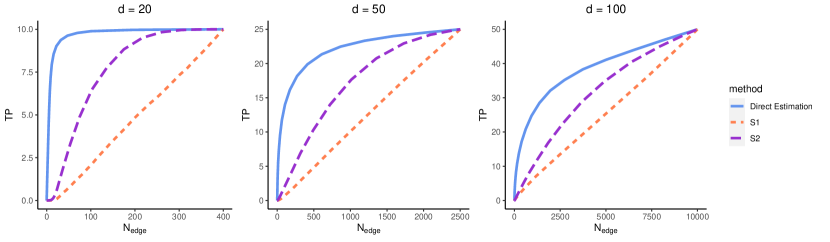
Figure 2: Comparison of the proposed direct estimation method with two separate estimation approaches in terms of $N_{\text{edge}}$ vs. TP. Here, $d=20,50,100$, $n_{1}=n_{2}=100$ and $|\Delta_{\Omega}|_{0}=0.4d$.

The estimators of $\Delta_{A}$ corresponding to S1 and S2 are, respectively, $\widehat{A}_{s1}^{(1)}-\widehat{A}_{s1}^{(2)}$ and $\widehat{A}_{s2}^{(1)}-\widehat{A}_{s2}^{(2)}$. For any estimator $\widehat{\Delta}_{A}$, we define

$$N_{\text{edge}}=\sum_{i,j=1,\ldots,d}I\left\{(\widehat{\Delta}_{A})_{ij}\neq 0\right\}~{}\mbox{and}~{}{\text{TP}}=\sum_{i,j=1,\ldots,d}I\left\{(\widehat{\Delta}_{A})_{ij}\neq 0~{}\mbox{and}~{}(\Delta_{A})_{ij}\neq 0\right\}.$$

Figure 2 shows $N_{\text{edge}}$ versus TP for all three methods. The curves were plotted using varying tuning parameters. Specifically, for the proposed direct estimator, with a fixed $\nu$ selected by the aBIC using an independent data set, the curve was plotted by varying $\lambda_{j}=\lambda$ for $j=1,\ldots,d$. The curves for the $l_{1}$-penalized approach (S1) and the $l_{1}$-constrained minimization approach (S2) were plotted by by varying $\eta_{1,1}=\eta_{1,2}=\eta$. Figure 2 clearly shows that the proposed direct estimator outperforms the separate estimation approaches. This is because $A^{(1)}$ and $A^{(2)}$ are not sparse, whereas $A^{(1)}-A^{(2)}$ is sparse. We also see that S2 performs better than S1. This may be because, as pointed out by Han et al. (2015), consistency of S2 requires weaker sparsity conditions on $A^{(1)}$ and $A^{(2)}$ than S1.

4.2 Simulation II

Next, we evaluate the finite sample performance of the proposed direct estimator under the VAR(2) model ${\bf x}^{(l)}_{t}={A_{1}^{(l)}}^{\intercal}{\bf x}_{t-1}+{A_{2}^{(l)}}^{\intercal}{\bf x}_{t-2}+{\mbox{\boldmath${\epsilon}$}}^{(l)}_{t}$ for $t>2$ and $l=1,2$. Here, $A^{(l)}_{1}$ and $A^{(l)}_{2}$ were generated similar to $A^{(l)}$ in Simulation I. Specifically, the support of $A^{(1)}_{1}$ was generated following the Bernoulli distribution with the success rate 0.5, and the values of the non-zero entries were then generated from a uniform distribution with support $[-0.8,-0.5]\bigcup[0.5,0.8]$.

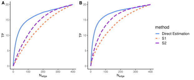
Figure 3: Comparison of the proposed direct estimation procedure with two separate estimation approaches in terms of $N_{\text{edge}}$ vs. TP. Here, $d=20$; (A): $\Delta_{A_{1}}$, (B): $\Delta_{A_{2}}$.

Similarly, the support of $A^{(1)}_{2}$ was generated following the Bernoulli distribution with the success rate 0.3, and the values of the non-zero entries were then generated from a uniform distribution with support $[-0.5,-0.3]\bigcup[0.3,0.5]$. We scaled the entries of $A^{(1)}_{1}$ and $A^{(1)}_{2}$ by $5$ and $3$, respectively. This ensures that the eigenvalues of the transition matrix of the lag 1 representation of the VAR(2) model in (3) have modulus less than 1, which, in turn, guarantees the stability of the VAR(2) processes $\{{\bf x}^{(1)}_{t}\}_{t\in\mathbb{N}}$. We then generated $A_{k}^{(2)}$ such that the largest $d$ (by magnitude) of $A^{(1)}_{k}$ entries change sign between $A^{(1)}_{k}$ and $A^{(2)}_{k}$, and then calculated $\Delta_{A_{k}}=A^{(1)}_{k}-A^{(2)}_{k}$ for $k=1,2$. By doing so, the eigenvalues of the transition matrix of lag 1 representation of the VAR(2) process $\{{\bf x}_{t}^{(2)}\}$ also have modulus less than 1. The elements in the error ${\mbox{\boldmath${\epsilon}$}}_{t}^{(l)}$ were independently generated from the normal distribution $N({0},0.1)$. The proposed direct estimation procedure was implemented based on the lag 1 reformulation in (3). Since the sparsity condition of $\Delta_{\Omega}$ is not satisfied for this reformulated model, this simulation study sheds light on how the proposed method performs when the sparsity condition of $\Delta_{\Omega}$ is violated. The separate estimation approach S1 was implemented directly based on the original VAR(2) model, while S2 was implemented based on the reformulated model, as suggested in Han et al. (2015).

We considered $d=20$; in this case, $\widetilde{A}^{(1)}$, $\widetilde{A}^{(2)}$ and their difference are all $40\times 40$ matrices. Similar to Fig. 2, Fig. 3 shows that the proposed direct estimator outperforms the separate estimation approaches in recovering the support of $\Delta_{A_{1}}$ and $\Delta_{A_{2}}$. This indicates the effectiveness of the proposed method under VAR(2) models even with non-sparse $\Delta_{\Omega}$.

4.3 Simulation III

In this simulation study, we examine the convergence rate in Theorem 1. We considered $\Sigma_{1}^{-1}=\left(0.4^{|i-j|}\right)_{i,j=1,\ldots,d}$, and let $S=\{(i,j)\mathrel{\mathop{\mathchar 58\relax}}|i-j|=1\mbox{ and }\max(i,j)\leq 11\}$. Then, $\Sigma_{2}^{-1}$ was obtained by changing the sign of the $(i,j)$-th entry of $\Sigma_{1}^{-1}$ for all $(i,j)\in S$. We further calculated $\Delta_{\Omega}=\Sigma_{1}^{-1}-\Sigma_{2}^{-1}$, leading to $|\Delta_{\Omega}|_{0}=20$ and $|\Delta_{\Omega}|_{1}=8$. We considered various $d$ and $n$ with $n_{1}=n_{2}=n$. For each pair of $d$ and $n$, we simulated random vectors ${\bf x}_{1}^{(l)},\ldots,{\bf x}_{n}^{(l)}$ according to the VAR(1) model ${\bf x}_{t}^{(l)}=A^{(l)^{\intercal}}{\bf x}_{t-1}^{(l)}+{\mbox{\boldmath${\epsilon}$}}_{t}^{(l)}$, where $A^{(l)}$ is the same as that in Simulation I, and ${\mbox{\boldmath${\epsilon}$}}_{t}^{(l)}$ follows the normal distribution $N({\bf 0},\Psi_{l})$ with $\Psi_{l}=\Sigma_{l}-A^{(l)\intercal}\Sigma_{l}A^{(l)}$. We then calculated the D-trace estimator $\widehat{\Delta}_{\Omega}(\nu)$ with $\nu$ proportional to $\left(\log d/n\right)^{1/2}$, as suggested in Theorem 1.

Figure 4 shows the behavior of the average Frobenius-norm error, $\left\|\widehat{\Delta}_{\Omega}(\nu)-\Delta_{\Omega}\right\|_{\text{F}}$, over 1000 replications for $n=200,300,\ldots,700$ and $d=25,125,625$. Each line in the figure corresponds to each value of $d$ and shows the Frobenius-norm error versus $(\log d/n)^{1/2}$. We see from the figure that all the points are approximately on a straight line. This is consistent with Theorem 1 in that the Frobenius norm error decays at the rate of $O\left((\log d/n)^{1/2}\right)$.

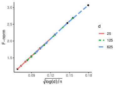
Figure 4: Lines of $\left\|\widehat{\Delta}_{\Omega}(\nu)-\Delta_{\Omega}\right\|_{\text{F}}$ vs. $\left(\log d/n\right)^{1/2}$ illustrate the convergence rate in Theorem 1. Here, $d=25,125,625;n=200,300,\ldots,700$; $|\Delta_{\Omega}|_{1}=8$.

5 EEG Data Analysis

In this section, we illustrate the proposed direct estimation approach using the EEG data shown in Fig. 1. Recall that the data set consists of EEG signals at 18 locations on the scalp of a patient diagnosed with left temporal lobe epilepsy during an epileptic seizure. The seizure affects the brain activity captured by the EEG signals. As shown in Fig. 1, the signals change at the time of the seizure ($t=85s$) and multiple later time points; we referred to these time points as change points hereafter. Safikhani and Shojaie (2020) analyzed this data set and identified eight change points with statistical guarantees at $t=83,111,114,121,130,138,144$ and $162s$. Since the EEG signals are unstable between $t=83s$ and $t=162s$, we aim to identify differential Granger causality between the time series with $t\leq 83s$ and those with $t\geq 162s$. Such changes may provide clinical insights into how the epileptic seizure impacts brain connectivity.

For ease of presentation, we denote the time series before $t=83s$ by ${X}^{(1)}=[{\bf x}^{(1)}_{1}\cdots{\bf x}^{(1)}_{n_{1}}]$ and after $t=162s$ by ${X}^{(2)}=[{\bf x}_{1}^{(2)}\cdots{\bf x}^{(2)}_{n_{2}}]$, where $n_{1}=8288$, $n_{2}=6590$, and each ${\bf x}_{j}^{(l)}\in\mathbb{R}^{18}$ for $l=1,2$ and $j=1,\ldots,n_{l}$. To speed up the computation, we downsampled each time series to include every tenth observation starting from the first time point; as a result, we reduced the number of time points in ${X}^{(l)}$ to $\widetilde{n}_{l}$ for $l=1,2$, where $\widetilde{n}_{1}=828$ and $\widetilde{n}_{2}=659$. We denote the reduced data by $\widetilde{X}^{(l)}=[\widetilde{\bf x}^{(l)}_{1}\cdots\widetilde{\bf x}^{(l)}_{\widetilde{n}_{l}}]$ and consider the following VAR(1) model:

$$\widetilde{\bf x}^{(l)}_{t}=A^{{(l)}\intercal}\widetilde{\bf x}^{(l)}_{t-1}+{\mbox{\boldmath${\epsilon}$}}_{t}^{(l)},~{}t=2,\ldots,\widetilde{n}_{l}~{}\mbox{and}~{}l=1,2.$$

Similar to Simulations I and II, we compared our direct estimation procedure with the separate estimation approaches (S1 and S2) in identifying nonzero entries of $\Delta_{A}=A^{(1)}-A^{(2)}$. For fair comparison, tuning parameters of all three methods were determined using aBIC, and all estimators were further thresholded at $0.05$.

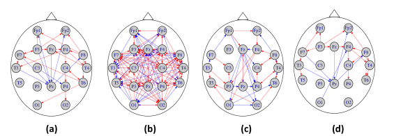
Figure 5: Networks showing differential Granger causality among the 18 EEG channels with blue and red edges representing positive and negative changes, respectively. The plots show the schematic locations of the EEG channels. Here, (a): direct estimation approach, (b): separate estimation approach based on the $l_{1}$-penalized least squares (S1), (c): separate estimation approach based on the $l_{1}$-constrained minimization (S2), and (d): stability selection based on the direct estimation approach with blue and red arrows representing edges with $m^{+}_{l_{1},l_{2}}$ and $m^{-}_{l_{1},l_{2}}$ being more than $50\%$, respectively.

Figure 5(a)-(c) show the plots of the estimates of $\Delta_{A}$ as networks, where each node represents a brain location, and directed edges between nodes represent nonzero entries in the estimator. In each network, the edges corresponding to the positive and negative entries of the estimator are shown in blue and red, respectively. Figure 5(a) shows the network obtained from the proposed direct estimation approach, highlighting the brain location “Pz" as critical to the seizure. This is consistent with the fact that “Pz" is in the site of epilepsy in this patient (Safikhani and Shojaie, 2020). However, such scientific insights cannot be gained from the dense network shown in Fig. 5(b). While Fig. 5(c) also shows a sparse network and shares some edges with Fig. 5(a), it, to some extent, highlights the brain location “Fz", which is not in the cite of epilepsy of this patient.

As our analyses are based on a reduced set of time points, we further validated our findings in Fig. 5(a) following an idea similar to the stability selection (Meinshausen and Bühlmann, 2010). Specifically, letting $\mathcal{S}_{i}=\{i+10(k-1)\mathrel{\mathop{\mathchar 58\relax}}k\in\mathbb{N}\}$ for $i=1,\ldots,10$, we denote $\widetilde{X}^{(l)}_{i}$ as the submatrix of $X^{(l)}$ with columns indexed by $\mathcal{S}_{i}\bigcap\{1,\ldots,n_{l}\}$ for $l=1,2$. For the $i$-th pair of data, i.e., $\widetilde{X}^{(1)}_{i}$ and $\widetilde{X}^{(2)}_{i}$, we estimated $\Delta_{A}$ using the proposed direct estimation procedure. The resulting estimator was further thresholded at 0.05, and we denote the thresholded estimator by $\widehat{\Delta}_{A}^{(i)}$. For $l_{1},l_{2}=1,\ldots,18$, we then calculate

$$m^{+}_{l_{1},l_{2}}=\frac{1}{10}\sum_{i=1}^{10}I\left\{\left(\widehat{\Delta}_{A}^{(i)}\right)_{l_{1},l_{2}}>0\right\}~{},~{}m^{-}_{l_{1},l_{2}}=\frac{1}{10}\sum_{i=1}^{10}I\left\{\left(\widehat{\Delta}_{A}^{(i)}\right)_{l_{1},l_{2}}<0\right\}.$$

Larger values of $m^{+}_{l_{1},l_{2}}$ or $m^{-}_{l_{1},l_{2}}$ indicate that the edge $l_{1}\rightarrow l_{2}$ is more likely present in the true $\Delta_{A}$. Figure 5(d) shows edges with $m^{+}_{l_{1},l_{2}}$ or $m^{-}_{l_{1},l_{2}}$ greater than $50\%$. It can be seen that the majority of the edges in Fig. 5(a), especially those related to “Pz", are also present in Fig. 5(d), further validating the importance of the brain location “Pz" to the seizure for this patient.

6 Discussions

We studied direct estimation of differential Granger causality between two high-dimensional VAR models. The proposed method does not require the sparsity of each transition matrix, requiring instead the sparsity of $\Delta_{\Omega}$ and $\Delta_{A}$. However, the sparsity assumption on $\Delta_{\Omega}$ may be less interpretable under VAR($p$) models with $p\geq 2$. Take $p=2$ as an example. According to the reformulated VAR(1) model in (3), we have $\Delta_{\Omega}=\left\{\mbox{cov}\left(\widetilde{\bf x}_{t}^{(1)}\right)\right\}^{-1}-\left\{\mbox{cov}\left(\widetilde{\bf x}_{t}^{(2)}\right)\right\}^{-1}$, where $\widetilde{\bf x}_{t}^{(l)}=\left({\bf x}_{t+1}^{(l)\intercal},{\bf x}_{t}^{(l)\intercal}\right)^{\intercal}$ for $l=1,2$. Letting $\Gamma^{(l)}(h)=\mbox{cov}\left({\bf x}_{t}^{(l)},{\bf x}_{t+h}^{(l)}\right)$ and $\Gamma^{(l)}(-h)=\{\Gamma^{(l)}(h)\}^{\intercal}$ for $h\in\mathbb{N}$,

$$\left\{\mbox{cov}\left(\widetilde{\bf x}_{t}^{(l)}\right)\right\}^{-1}=\begin{pmatrix}\Xi_{1}^{(l)}&-\Xi_{1}^{(l)}\Gamma^{(l)}(-1)\{\Gamma^{(l)}(0)\}^{-1}\\ -\{\Gamma^{(l)}(0)\}^{-1}\Gamma^{(l)}(1)\Xi_{1}^{(l)}&\Xi_{2}^{(l)}\end{pmatrix},$$

where $\Xi_{1}^{(l)}=[\Gamma^{(l)}(0)-\Gamma^{(l)}(-1)\{\Gamma^{(l)}(0)\}^{-1}\Gamma^{(l)}(1)]^{-1}$ and $\Xi_{2}^{(l)}=[\Gamma^{(l)}(0)-\Gamma^{(l)}(1)\{\Gamma^{(l)}(0)\}^{-1}\Gamma^{(l)}(-1)]^{-1}$. Thus, the sparsity of $\Delta_{\Omega}$ implies the sparsity of $\Xi_{k}^{(1)}-\Xi_{k}^{(2)}$ for $k=1,2$, which is hard to interpret. It would be interesting to develop alternative methods for direct estimation of differential Granger causality under VAR($p$) models with $p\geq 2$.

7 Appendix

7.1 Proof of Main results

In this section, we provide proofs for Theorems 1-4 in the main text. Throughout, we assume the order of the VAR model, $p$, is fixed, but the dimension $d$ is allowed to grow with the sample size $n$. The first lemma characterizes the convergence rate of the lag-$h$ auto-covariance matrix of a stationary time series in terms of the element-wise norm.

Lemma 1.

Consider $d$-dimensional random vectors ${\bf z}_{1},\ldots,{\bf z}_{n}$ sampled from a stationary time series $\{{\bf z}_{t}\}_{t\in\mathbb{N}}$, where ${\bf z}_{t}\in\mathbb{R}^{d}$ and $E({\bf z}_{t})=0$. Suppose that $\{{\bf z}_{t}\}_{t\in\mathbb{N}}$ satisfies Assumption 1 with the spectral density function $f(\cdot)$. For any non-negative integer $h$, let $\Gamma(h)=E({\bf z}_{t}{\bf z}_{t+h}^{\intercal})$, $\widehat{\Gamma}(h)=(n-h)^{-1}\sum_{t=1}^{n-h}{\bf z}_{t}{\bf z}_{t+h}^{\intercal}$, $\Gamma(-h)=\Gamma(h)^{\intercal}$ and $\widehat{\Gamma}(-h)=\widehat{\Gamma}(h)^{\intercal}$. If $d>1$ and $n\geq 24\log d+h$, then with probability at least $1-8d^{-1}$, we have

$$\|\widehat{\Gamma}(h)-\Gamma(h)\|_{\max} ~{}\leq 32\pi\left(\frac{6\log d}{n-h}\right)^{1/2}\mathcal{M}(f),$$

$$\|\widehat{\Gamma}(-h)-\Gamma(-h)\|_{\max} ~{}\leq 32\pi\left(\frac{6\log d}{n-h}\right)^{1/2}\mathcal{M}(f),$$

where $\mathcal{M}(f)$ is defined in Assumption 1.

Proof.

Since $\Gamma(-h)=\Gamma(h)^{\intercal}$, we only prove the first inequality. For $j,k=1,\ldots,d$, let $\sigma_{jk,h}$ and $\widehat{\sigma}_{jk,h}$, respectively, denote the $(j,k)$-th entry of $\Gamma(h)$ and $\widehat{\Gamma}(h)$. Then, for all $\eta>0$, we have

$$~{}\mbox{pr}\left(\left|\sigma_{jk,h}-\widehat{\sigma}_{jk,h}\right|>\eta\right)=\mbox{pr}\left(\left|(n-h)^{-1}\sum_{t=1}^{n-h}{z}_{tj}{z}_{t+h,k}-\sigma_{jk,h}\right|>\eta\right)$$

$$= ~{}\mbox{pr}\left(\left|\{4(n-h)\}^{-1}\left\{\sum_{t=1}^{n-h}({z}_{tj}+{z}_{t+h,k})^{2}-\sum_{t=1}^{n-h}({z}_{tj}-{z}_{t+h,k})^{2}\right\}-\sigma_{jk,h}\right|>\eta\right)$$

$$\leq ~{}\mbox{pr}\left(\left|(n-h)^{-1}\sum_{t=1}^{n-h}({z}_{tj}+{z}_{t+h,k})^{2}-(\sigma_{jj,h}+\sigma_{kk,h}+2\sigma_{jk,h})\right|>2\eta\right)$$

$$+ ~{}\mbox{pr}\left(\left|(n-h)^{-1}\sum_{t=1}^{n-h}({z}_{tj}-{z}_{t+h,k})^{2}-(\sigma_{jj,h}+\sigma_{kk,h}-2\sigma_{jk,h})\right|>2\eta\right).$$

Note that $({z}_{1j}+{z}_{1+h,k},{z}_{2j}+{z}_{2+h,k},\ldots,{z}_{n-h,j}+{z}_{n,k})^{\intercal}\sim N(0,Q_{h})$ where for $i,l=1,\ldots,n-h$, the $(i,l)$-th entry of $Q_{h}$ takes the following form:

$$Q_{il,h}= ~{}\mbox{cov}({z}_{ij}+{z}_{i+h,k},{z}_{lj}+{z}_{l+h,k})$$

$$= ~{}\Gamma(l-i)_{jj}+\Gamma(l-i+h)_{jk}+\Gamma(l-i)_{kk}+\Gamma(l-i-h)_{kj}$$

$$= ~{}{\bf v}_{j}^{\intercal}\Gamma(l-i){\bf v}_{j}+{\bf v}_{j}^{\intercal}\Gamma(l-i+h){\bf v}_{k}+{\bf v}_{k}^{\intercal}\Gamma(l-i){\bf v}_{k}+{\bf v}_{k}^{\intercal}\Gamma(l-i-h){\bf v}_{j}$$

and where ${\bf v}_{j}\in\mathbb{R}^{d}$ is a vector with a one in its $j$-th entry and zeros elsewhere. Define

$$\Upsilon_{n}=\begin{bmatrix}\Gamma(0)&\Gamma(1)&\Gamma(2)&\dots&\Gamma(n-1)\\ \Gamma(-1)&\Gamma(0)&\Gamma(1)&\dots&\Gamma(n-2)\\ \vdots&\vdots&\vdots&\ddots&\vdots\\ \Gamma(1-n)&\Gamma(2-n)&\Gamma(3-n)&\dots&\Gamma(0)\end{bmatrix}.$$ (18)

For any ${\bf w}\in\mathbb{R}^{n-h}$ with $\|{\bf w}\|_{2}=1$, we have

$${\bf w}^{\intercal}Q_{h}{\bf w}= ~{}\sum_{r=1}^{n-h}\sum_{s=1}^{n-h}w_{r}w_{s}Q_{rs,h}$$

$$= ~{}\sum_{r=1}^{n-h}\sum_{s=1}^{n-h}w_{r}w_{s}{\bf v}_{j}^{\intercal}\Gamma(s-r){\bf v}_{j}+\sum_{r=1}^{n-h}\sum_{s=1}^{n-h}w_{r}w_{s}{\bf v}_{k}^{\intercal}\Gamma(s-r){\bf v}_{k}+$$

$$~{}\sum_{r=1}^{n-h}\sum_{s=1}^{n-h}w_{r}w_{s}{\bf v}_{j}^{\intercal}\Gamma(s-r+h){\bf v}_{k}+\sum_{r=1}^{n-h}\sum_{s=1}^{n-h}w_{r}w_{s}{\bf v}_{k}^{\intercal}\Gamma(s-r-h){\bf v}_{j}.$$ (19)

Letting

$$\widetilde{\bf w}_{1}=\left({\bf w}^{\intercal},\underbrace{0,\ldots,0}_{h}\right)^{\intercal},~{}\widetilde{\bf w}_{2}=\left(\underbrace{0,\ldots,0}_{h},{\bf w}^{\intercal}\right)^{\intercal},$$

one can check that

$$~{}\sum_{r=1}^{n-h}\sum_{s=1}^{n-h}w_{r}w_{s}{\bf v}_{j}^{\intercal}\Gamma(s-r){\bf v}_{j}=(\widetilde{\bf w}_{1}\otimes{\bf v}_{j})^{\intercal}\Upsilon_{n}(\widetilde{\bf w}_{1}\otimes{\bf v}_{j}),$$

$$~{}\sum_{r=1}^{n-h}\sum_{s=1}^{n-h}w_{r}w_{s}{\bf v}_{k}^{\intercal}\Gamma(s-r){\bf v}_{k}=(\widetilde{\bf w}_{1}\otimes{\bf v}_{k})^{\intercal}\Upsilon_{n}(\widetilde{\bf w}_{1}\otimes{\bf v}_{k}),$$

$$~{}\sum_{r=1}^{n-h}\sum_{s=1}^{n-h}w_{r}w_{s}{\bf v}_{j}^{\intercal}\Gamma(s-r+h){\bf v}_{k}=(\widetilde{\bf w}_{1}\otimes{\bf v}_{j})^{\intercal}\Upsilon_{n}(\widetilde{\bf w}_{2}\otimes{\bf v}_{k}),$$

$$~{}\sum_{r=1}^{n-h}\sum_{s=1}^{n-h}w_{r}w_{s}{\bf v}_{k}^{\intercal}\Gamma(s-r-h){\bf v}_{j}=(\widetilde{\bf w}_{2}\otimes{\bf v}_{k})^{\intercal}\Upsilon_{n}(\widetilde{\bf w}_{1}\otimes{\bf v}_{j}).$$

Since $\|\widetilde{\bf w}_{1}\otimes{\bf v}_{j}\|_{2}=1,\|\widetilde{\bf w}_{1}\otimes{\bf v}_{k}\|_{2}=1,\|\widetilde{\bf w}_{2}\otimes{\bf v}_{j}\|_{2}=1$, and $\|\widetilde{\bf w}_{2}\otimes{\bf v}_{k}\|_{2}=1$, we have

$${\bf w}^{\intercal}Q_{h}{\bf w}\leq 4\lambda_{\max}(\Upsilon_{n}),$$

where $\lambda_{\max}(\Upsilon_{n})$ denotes the largest eigenvalue of $\Upsilon_{n}$. Thus, using Lemma 6 in Section S.2, we get $\|Q_{h}\|_{2}\leq 4\lambda_{\max}(\Upsilon_{n})\leq 8\pi\mathcal{M}(f)$, where $\mathcal{M}(f)$ is defined in Assumption 1. Then, using Lemma 7 in Section S.2, for $\eta\geq 32\pi(n-h)^{-1/2}\mathcal{M}(f)$, we get

$$~{}\mbox{pr}\left(\left|(n-h)^{-1}\sum_{t=1}^{n-h}({z}_{tj}+{z}_{t+h,k})^{2}-(\sigma_{jj,h}+\sigma_{kk,h}+2\sigma_{jk,h})\right|>2\eta\right)$$

$$\leq ~{}2\exp\left[-\frac{n-h}{2}\left\{\frac{\eta}{16\pi\mathcal{M}(f)}-2(n-h)^{-1/2}\right\}^{2}\right]+2\exp\left(-\frac{n-h}{2}\right).$$ (20)

Using a similar argument, we have

$$~{}\mbox{pr}\left(\left|(n-h)^{-1}\sum_{t=1}^{n-h}({z}_{tj}-{z}_{t+h,k})^{2}-(\sigma_{jj,h}+\sigma_{kk,h}-2\sigma_{jk,h})\right|>2\eta\right)$$

$$\leq ~{}2\exp\left[-\frac{n-h}{2}\left\{\frac{\eta}{16\pi\mathcal{M}(f)}-2(n-h)^{-1/2}\right\}^{2}\right]+2\exp\left(-\frac{n-h}{2}\right).$$ (21)

Combining (7.1) and (7.1) and applying the union bound, we have

$$\mbox{pr}\left(\|\Gamma(h)-\widehat{\Gamma}(h)\|_{\max}>\eta\right)\leq ~{}4d^{2}\exp\left(-\frac{n-h}{2}\right)$$

$$+ ~{}4d^{2}\exp\left[-\frac{n-h}{2}\left\{\frac{\eta}{16\pi\mathcal{M}(f)}-2(n-h)^{-1/2}\right\}^{2}\right].$$ (22)

Taking $\eta=32\pi\mathcal{M}(f)\{6(n-h)^{-1}\log d\}^{1/2}$, when $d>1$ and $n\geq 24\log d+h$, it can be checked that $6\log d>1$ and

$$1\geq\left|\frac{\eta}{16\pi\mathcal{M}(f)}-2(n-h)^{-1/2}\right|\geq\left(\frac{6\log d}{n-h}\right)^{1/2}.$$

Therefore, we have

$$\mbox{pr}\left(\|\Gamma(h)-\widehat{\Gamma}(h)\|_{\max}>\eta\right)\leq 8d^{2}\exp\left[-\frac{(n-h)}{2}\left\{\frac{\eta}{16\pi\mathcal{M}(f)}-2(n-h)^{-1/2}\right\}^{2}\right]\leq 8d^{-1}.$$

This completes the proof. ∎

Under the reformulated VAR($p$) model $\widetilde{\bf x}_{t}^{(l)}=\widetilde{A}^{(l)\intercal}\widetilde{\bf x}^{(l)}_{t-1}+\widetilde{{\mbox{\boldmath${\epsilon}$}}}_{t}^{(l)}$ for $l=1,2$, we have

$$\Sigma_{l}=\mbox{cov}\left(\widetilde{\bf x}^{(l)}_{t}\right)=\begin{bmatrix}\Gamma(0)&\Gamma(-1)&\Gamma(-2)&\dots&\Gamma(1-p)\\ \Gamma(1)&\Gamma(0)&\Gamma(-1)&\dots&\Gamma(2-p)\\ \vdots&\vdots&\vdots&\ddots&\vdots\\ \Gamma(p-1)&\Gamma(p-2)&\Gamma(p-3)&\dots&\Gamma(0)\end{bmatrix}$$

and

$$\widehat{\Sigma}_{l}=\widehat{\mbox{cov}}\left(\widetilde{\bf x}^{(l)}_{t}\right)=\begin{bmatrix}\widehat{\Gamma}(0)&\widehat{\Gamma}(-1)&\widehat{\Gamma}(-2)&\dots&\widehat{\Gamma}(1-p)\\ \widehat{\Gamma}(1)&\widehat{\Gamma}(0)&\widehat{\Gamma}(-1)&\dots&\widehat{\Gamma}(2-p)\\ \vdots&\vdots&\vdots&\ddots&\vdots\\ \widehat{\Gamma}(p-1)&\widehat{\Gamma}(p-2)&\widehat{\Gamma}(p-3)&\dots&\widehat{\Gamma}(0)\end{bmatrix}.$$

Recall that $C_{M}=\max(\mathcal{M}(f_{1}),\mathcal{M}(f_{2}))$ and $C_{\Sigma}=\max(\|\Sigma_{1}\|_{\max},\|\Sigma_{2}\|_{\max})$. Also, denote

$$\xi(n_{1},n_{2},d,p)=C_{M}\left(\frac{6\log d}{\min(n_{1},n_{2})-p}\right)^{1/2}.$$

In the next lemma, we prove that $\widehat{\Sigma}_{1}\otimes\widehat{\Sigma}_{2}$ satisfies a modified restricted eigenvalue (RE) condition (Loh and Wainwright, 2012) with high probability.

Lemma 2.

Suppose that ${\bf x}_{t}^{(l)}$ satisfies Assumption 1 with the spectral density function $f_{l}(\cdot)$ for $l=1,2$. If

$$\min(n_{1},n_{2})\geq\max\left\{6144\pi^{2}\max\left(\mathcal{M}^{2}(f_{1})/\|\Sigma_{1}\|_{\max}^{2},\mathcal{M}^{2}(f_{2})/\|\Sigma_{2}\|_{\max}^{2}\right),1\right\}\log d+(p-1),$$

then with probability at least $1-16d^{-1}$, for all ${\bf m}\in\mathbb{R}^{d^{2}}$, we have

$${\bf m}^{\intercal}\left(\widehat{\Sigma}_{1}\otimes\widehat{\Sigma}_{2}\right){\bf m}\geq\lambda_{\min}(\Sigma_{1})\lambda_{\min}(\Sigma_{2})\|{\bf m}\|_{2}^{2}-32\pi C_{\Sigma}\xi(n_{1},n_{2},d,p-1)\|{\bf m}\|_{1}^{2}.$$

Proof.

First, note that

$$\|\widehat{\Sigma}_{1} ~{}\otimes\widehat{\Sigma}_{2}-{\Sigma}_{1}\otimes{\Sigma}_{2}\|_{\max}\leq$$ (23)

$$~{}\|\Sigma_{1}\|_{\max}\|\widehat{\Sigma}_{2}-\Sigma_{2}\|_{\max}+\|\Sigma_{2}\|_{\max}\|\widehat{\Sigma}_{1}-{\Sigma}_{1}\|_{\max}+\|\widehat{\Sigma}_{1}-{\Sigma}_{1}\|_{\max}\|\widehat{\Sigma}_{2}-{\Sigma}_{2}\|_{\max}.$$

By Lemma 1, we know that there exists an event $\mathcal{A}_{1}$ with $\mbox{pr}(\mathcal{A}_{1})\geq 1-16d^{-1}$ such that on the event $\mathcal{A}_{1}$,

$$\|\Sigma_{1}\|_{\max}\|\widehat{\Sigma}_{2}-\Sigma_{2}\|_{\max}+\|\Sigma_{2}\|_{\max}\|\widehat{\Sigma}_{1}-{\Sigma}_{1}\|_{\max}\leq 32\pi C_{\Sigma}\xi(n_{1},n_{2},d,p-1);$$ (24)

here, we use the fact that $\|\widehat{\Sigma}_{l}-\Sigma_{l}\|=\max_{h=0,\ldots,p-1}\|\widehat{\Gamma}(h)-\Gamma(h)\|_{\max}$ for $l=1,2$. Similarly, on the event $\mathcal{A}_{1}$,

$$\|\widehat{\Sigma}_{1}-{\Sigma}_{1}\|_{\max}\|\widehat{\Sigma}_{2}-{\Sigma}_{2}\|_{\max}\leq 6144\pi^{2}\mathcal{M}(f_{1})\mathcal{M}(f_{2})\log d\big{\{}(n_{1}-p+1)(n_{2}-p+1)\big{\}}^{-1/2}.$$ (25)

It is easy to check that when $\min(n_{1},n_{2})\geq 6144\pi^{2}\log d\max\left(\mathcal{M}^{2}(f_{1})/\|\Sigma_{1}\|_{\max}^{2},\mathcal{M}^{2}(f_{2})/\|\Sigma_{2}\|_{\max}^{2}\right)+(p-1)$, $\mbox{RHS of (\ref{lemma2:pf3})}\leq\mbox{RHS of (\ref{lemma2:pf2})};$ this leads to the $\mbox{RHS of (\ref{lemma2:pf1})}\leq 64\pi C_{\Sigma}\xi(n_{1},n_{2},d,p-1).$ Thus, on the event $\mathcal{A}_{1}$, for any ${\bf m}\in\mathbb{R}^{d^{2}}$, we have

$${\bf m}^{\intercal}\left(\widehat{\Sigma}_{1}\otimes\widehat{\Sigma}_{2}\right){\bf m}= ~{}{\bf m}^{\intercal}\left({\Sigma}_{1}\otimes{\Sigma}_{2}\right){\bf m}+{\bf m}^{\intercal}\left(\widehat{\Sigma}_{1}\otimes\widehat{\Sigma}_{2}-{\Sigma}_{1}\otimes{\Sigma}_{2}\right){\bf m}$$

$$\geq ~{}{\bf m}^{\intercal}\left({\Sigma}_{1}\otimes{\Sigma}_{2}\right){\bf m}-\left|{\bf m}^{\intercal}\left(\widehat{\Sigma}_{1}\otimes\widehat{\Sigma}_{2}-{\Sigma}_{1}\otimes{\Sigma}_{2}\right){\bf m}\right|$$

$$\geq ~{}{\bf m}^{\intercal}\left({\Sigma}_{1}\otimes{\Sigma}_{2}\right){\bf m}-\left\|\widehat{\Sigma}_{1}\otimes\widehat{\Sigma}_{2}-{\Sigma}_{1}\otimes{\Sigma}_{2}\right\|_{\max}\|{\bf m}\|_{1}^{2}$$

$$\geq ~{}\lambda_{\min}(\Sigma_{1})\lambda_{\min}(\Sigma_{2})\|{\bf m}\|_{2}^{2}-\left\|\widehat{\Sigma}_{1}\otimes\widehat{\Sigma}_{2}-{\Sigma}_{1}\otimes{\Sigma}_{2}\right\|_{\max}\|{\bf m}\|_{1}^{2}$$

$$\geq ~{}\lambda_{\min}(\Sigma_{1})\lambda_{\min}(\Sigma_{2})\|{\bf m}\|_{2}^{2}-64\pi C_{\Sigma}\xi(n_{1},n_{2},d,p-1)\|{\bf m}\|_{1}^{2},$$

where we use the fact that $\lambda_{\min}(\Sigma_{1}\otimes\Sigma_{2})=\lambda_{\min}(\Sigma_{1})\lambda_{\min}(\Sigma_{2})$. This completes the proof. ∎

The next lemma provides an element-wise bound for $0.5(\widehat{\Sigma}_{1}\Delta_{\Omega}\widehat{\Sigma}_{2}+\widehat{\Sigma}_{2}\Delta_{\Omega}\widehat{\Sigma}_{1})-(\widehat{\Sigma}_{1}-\widehat{\Sigma}_{2})$, which is the derivative of $L_{D}(\cdot)$ with respect to $\Delta_{\Omega}$.

Lemma 3.

Suppose that ${\bf x}_{t}^{(l)}$ satisfies Assumption 1 with the spectral density function $f_{l}(\cdot)$ for $l=1,2$. If $d>1$ and

$$\min(n_{1},n_{2})\geq\max\left(6144\pi^{2}\max\left(\mathcal{M}^{2}(f_{1})/\|\Sigma_{1}\|_{\max}^{2},\mathcal{M}^{2}(f_{2})/\|\Sigma_{2}\|_{\max}^{2}\right),1\right)\log d+p-1,$$

then with probability at least $1-16d^{-1}$, we have

$$\left\|0.5\left(\widehat{\Sigma}_{1}\Delta_{\Omega}\widehat{\Sigma}_{2}+\widehat{\Sigma}_{2}\Delta_{\Omega}\widehat{\Sigma}_{1}\right)-\left(\widehat{\Sigma}_{1}-\widehat{\Sigma}_{2}\right)\right\|_{\max}\leq 64\pi\xi(n_{1},n_{2},d,p-1)(1+C_{\Sigma}|\Delta_{\Omega}|_{1}).$$

Proof.

Denoting $\Gamma=0.5\left(\Sigma_{2}\otimes\Sigma_{1}+\Sigma_{1}\otimes\Sigma_{2}\right)$ and $\widehat{\Gamma}=0.5\left(\widehat{\Sigma}_{2}\otimes\widehat{\Sigma}_{1}+\widehat{\Sigma}_{1}\otimes\widehat{\Sigma}_{2}\right)$, it can be seen that

$$\left\|0.5\left(\widehat{\Sigma}_{1}\Delta_{\Omega}\widehat{\Sigma}_{2}+\widehat{\Sigma}_{2}\Delta_{\Omega}\widehat{\Sigma}_{1}\right)-\left(\widehat{\Sigma}_{1}-\widehat{\Sigma}_{2}\right)\right\|_{\max}=\left\|\widehat{\Gamma}\mbox{vec}(\Delta_{\Omega})-\left\{\mbox{vec}\left(\widehat{\Sigma}_{1}\right)-\mbox{vec}\left(\widehat{\Sigma}_{2}\right)\right\}\right\|_{\max}.$$ (26)

Recall from eq. (8) in the main text that $\Gamma\mbox{vec}(\Delta_{\Omega})-\left(\mbox{vec}(\Sigma_{1})-\mbox{vec}(\Sigma_{2})\right)=0.$ Hence,

$$\mbox{RHS of (\ref{lemma3:pf1})}\leq ~{}\left\|\left(\widehat{\Gamma}-\Gamma\right)\mbox{vec}(\Delta_{\Omega})\right\|_{\max}+\sum_{l=1}^{2}\left\|\widehat{\Sigma}_{l}-\Sigma_{l}\right\|_{\max}$$

$$\leq \|\widehat{\Gamma}-\Gamma\|_{\max}|\Delta_{\Omega}|_{1}+\sum_{l=1}^{2}\left\|\widehat{\Sigma}_{l}-\Sigma_{l}\right\|_{\max}.$$ (27)

Using Lemmas 1 and 2, we know that on the event $\mathcal{A}_{1}$, since

$$\min(n_{1},n_{2})\geq\max\left(6144\pi^{2}\max\left(\mathcal{M}^{2}(f_{1})/\|\Sigma_{1}\|_{\max}^{2},\mathcal{M}^{2}(f_{2})/\|\Sigma_{2}\|_{\max}^{2}\right),1\right)\log d+p-1,$$

we have

$$\sum_{l=1}^{2}\left\|\widehat{\Sigma}_{l}-\Sigma_{l}\right\|_{\max}\leq 64\pi\xi(n_{1},n_{2},d,p-1).$$

Also, using similar techniques to (23)-(25), one can show

$$\left\|(\widehat{\Gamma}-\Gamma)\mbox{vec}(\Delta_{\Omega})\right\|_{\max}\leq 64\pi C_{\Sigma}\xi(n_{1},n_{2},d,p-1)|\Delta_{\Omega}|_{1}.$$

Therefore, $\mbox{RHS of (\ref{lemma3:pf2})}\leq 64\pi\xi(n_{1},n_{2},d,p-1)(1+C_{\Sigma}|\Delta_{\Omega}|_{1}),$ as claimed. ∎

Our penalized D-trace estimator of $\Delta_{\Omega}$,

$$\widehat{\Delta}_{\Omega}(\nu)=\mbox{argmin}_{\Delta_{\Omega}}L_{\mathrm{D}}\left(\Delta_{\Omega},\widehat{\Sigma}_{1},\widehat{\Sigma}_{2}\right)+\nu|\Delta_{\Omega}|_{1},$$

is an $l_{1}$-penalized $M$-estimator. We now prove consistency of $\widehat{\Delta}_{\Omega}(\nu)$ using the general framework proposed in Negahban et al. (2012); a brief introduction of this framework adapted to our setting is given in Section S.2.

We now proof Theorem 1.

Proof.

First, recall that the Hessian matrix of the D-trace loss function is $0.5(\widehat{\Sigma}_{1}\otimes\widehat{\Sigma}_{2}+\widehat{\Sigma}_{2}\otimes\widehat{\Sigma}_{1})$, and $S_{\Omega}$ is the support of the true $\Delta_{\Omega}$. Let $S_{\Omega}^{c}$ denote the compliment set of $S_{\Omega}$. Consider ${\bf m}\in\mathcal{C}(S_{\Omega})$, where $\mathcal{C}(S_{\Omega})=\{{\mbox{\boldmath${\theta}$}}\mathrel{\mathop{\mathchar 58\relax}}\|{\mbox{\boldmath${\theta}$}}_{S_{\Omega}^{c}}\|_{1}\leq 3\|{\mbox{\boldmath${\theta}$}}\|_{S_{\Omega}}\}$. Then, $\|{\bf m}\|_{1}\leq 4\|{\bf m}_{S_{\Omega}}\|_{1}\leq 4\sqrt{s_{\Omega}}\|{\bf m}_{S_{\Omega}}\|_{2}$. Therefore, using Lemma 2, we have, on the event $\mathcal{A}_{1}$,

$$~{}{\bf m}^{\intercal}\left\{0.5(\widehat{\Sigma}_{1}\otimes\widehat{\Sigma}_{2}+\widehat{\Sigma}_{2}\otimes\widehat{\Sigma}_{1})\right\}{\bf m}$$

$$\geq ~{}\left\{\lambda_{\min}(\Sigma_{1})\lambda_{\min}(\Sigma_{2})-1024\pi s_{\Omega}C_{\Sigma}\xi(n_{1},n_{2},d,p-1)\right\}\|{\bf m}\|_{2}^{2}.$$

For ease of notation, let

$$C_{G}=6\times\left\{2048\pi C_{M}C_{\Sigma}\lambda_{\min}^{-1}(\Sigma_{1})\lambda_{\min}^{-1}(\Sigma_{2})\right\}^{2}.$$ (28)

For $\min(n_{1},n_{2})\geq C_{G}s_{\Omega}^{2}\log d+p-1,$ on the event $\mathcal{A}_{1}$, we have

$${\bf m}^{\intercal}\left\{0.5(\widehat{\Sigma}_{1}\otimes\widehat{\Sigma}_{2}+\widehat{\Sigma}_{2}\otimes\widehat{\Sigma}_{1})\right\}{\bf m}\geq\frac{1}{2}\lambda_{\min}(\Sigma_{1})\lambda_{\min}(\Sigma_{2})\|{\bf m}\|_{2}^{2}.$$

Thus, with the probability approaching 1, the D-trace loss function satisfies the restricted eigenvalue condition (see Condition A1 in Section S2) with $\kappa_{1}=0.5\lambda_{\min}(\Sigma_{1})\lambda_{\min}(\Sigma_{2})$ and $S^{*}=S_{\Omega}$.

Recall that $\nabla L_{D}(\Delta_{\Omega},\widehat{\Sigma}_{1},\widehat{\Sigma}_{2})=0.5(\widehat{\Sigma}_{1}\Delta_{\Omega}\widehat{\Sigma}_{2}+\widehat{\Sigma}_{2}\Delta_{\Omega}\widehat{\Sigma}_{1})-(\widehat{\Sigma}_{1}-\widehat{\Sigma}_{2})$. Since $\nu\geq 2\|\nabla L_{D}(\Delta_{\Omega},\widehat{\Sigma}_{1},\widehat{\Sigma}_{2})\|_{\max}$ (Lemma 3), Using Lemma 8 in Section S2, we have

$$\|\widehat{\Delta}_{\Omega}(\nu)-\Delta_{\Omega}\|_{\text{F}}\leq\frac{6\nu\sqrt{s_{\Omega}}}{\lambda_{\min}(\Sigma_{1})\lambda_{\min}(\Sigma_{2})};$$

here, we use the fact that $\Psi(S_{\Omega})=\sqrt{s_{\Omega}}$. This completes the proof. ∎

Recall that the Hessian matrix of the loss function $L_{A}(\cdot)$ with respect to $\Delta_{A}$ is $\Sigma_{1}+\Sigma_{2}$. In the next lemma, we establish the restricted eigenvalue condition (Condition A1) for $\widehat{\Sigma}_{1}+\widehat{\Sigma}_{2}$ with high probability.

Lemma 4.

Suppose that ${\bf x}_{t}^{(l)}$ satisfies Assumption 1 with the spectral density function $f_{l}(\cdot)$ for $l=1,2$. If $d>1$ and $\min(n_{1},n_{2})\geq 24\log d+p-1$, then with probability at least $1-16d^{-1}$, we have

$${\bf m}^{\intercal}\left(\widehat{\Sigma}_{1}+\widehat{\Sigma}_{2}\right){\bf m}\geq\left\{\lambda_{\min}(\Sigma_{1})+\lambda_{\min}(\Sigma_{2})\right\}\|{\bf m}\|_{2}^{2}-64\pi\xi(n_{1},n_{2},d,p-1)\|{\bf m}\|_{1}^{2},~{}\mbox{for all}~{}{\bf m}\in\mathbb{R}^{d}.$$

Proof.

This proof is similar to that for Lemma 2. Thus, we only present the key steps below. First, using Lemma 1, we know that on the $\mathcal{A}_{1}$, when $d>1$ and $\min(n_{1},n_{2})\geq 24\log d+p-1$, we have

$$~{}\|\widehat{\Sigma}_{2}-\Sigma_{2}\|_{\max}+\|\widehat{\Sigma}_{1}-{\Sigma}_{1}\|_{\max}\leq 64\pi\xi(n_{1},n_{2},d,p-1).$$

Thus, for any ${\bf m}\in\mathbb{R}^{d}$,

$${\bf m}^{\intercal}\left(\widehat{\Sigma}_{1}+\widehat{\Sigma}_{2}\right){\bf m}\geq ~{}\left\{\lambda_{\min}(\Sigma_{1})+\lambda_{\min}(\Sigma_{2})\right\}\|{\bf m}\|_{2}^{2}-\left(\left\|\widehat{\Sigma}_{1}-{\Sigma}_{1}\right\|_{\max}+\left\|\widehat{\Sigma}_{2}-\Sigma_{2}\right\|_{\max}\right)\|{\bf m}\|_{1}^{2}$$

$$\geq ~{}\left\{\lambda_{\min}(\Sigma_{1})+\lambda_{\min}(\Sigma_{2})\right\}\|{\bf m}\|_{2}^{2}-64\pi\xi(n_{1},n_{2},d,p-1)\|{\bf m}\|_{1}^{2},$$

which completes the proof. ∎

Next, recall that

$$\Theta_{l}=E\left(\widetilde{\bf x}_{t}^{(l)}\widetilde{\bf x}_{t+1}^{(l)}\right)=\begin{bmatrix}\Gamma(1)&\Gamma(0)&\Gamma(-1)&\dots&\Gamma(2-p)\\ \Gamma(2)&\Gamma(1)&\Gamma(0)&\dots&\Gamma(3-p)\\ \vdots&\vdots&\vdots&\ddots&\vdots\\ \Gamma(p)&\Gamma(p-1)&\Gamma(p-2)&\dots&\Gamma(1)\end{bmatrix},$$

and

$$\widehat{\Theta}_{l}=\widehat{E}\left(\widetilde{\bf x}_{t}^{(l)}\widetilde{\bf x}_{t+1}^{(l)}\right)=\begin{bmatrix}\widehat{\Gamma}(1)&\widehat{\Gamma}(0)&\widehat{\Gamma}(-1)&\dots&\widehat{\Gamma}(2-p)\\ \widehat{\Gamma}(2)&\widehat{\Gamma}(1)&\widehat{\Gamma}(0)&\dots&\widehat{\Gamma}(3-p)\\ \vdots&\vdots&\vdots&\ddots&\vdots\\ \widehat{\Gamma}(p)&\widehat{\Gamma}(p-1)&\widehat{\Gamma}(p-2)&\dots&\widehat{\Gamma}(1)\end{bmatrix}$$

for $l=1,2$. Also, recall that ${\mbox{\boldmath${\beta}$}}_{j}$ and ${\bf w}_{j}$, respectively, denote the $j$-th column of $\Delta_{A}$ and $\Sigma_{1}\Delta_{\Omega}\Theta_{2}+\Sigma_{2}\Delta_{\Omega}\Theta_{1}+2(\Theta_{1}-\Theta_{2})$. The next lemma provides a uniform bound for the entries in $(\widehat{\Sigma}_{1}+\widehat{\Sigma}_{2}){\mbox{\boldmath${\beta}$}}_{j}-\widehat{\bf w}_{j}$, which is the derivative of $L_{A}(\cdot)$ with respect to ${\mbox{\boldmath${\beta}$}}_{j}$.

Lemma 5.

Suppose that ${\bf x}_{t}^{(l)}$ satisfies Condition 1 in the main text with the spectral density function $f_{l}(\cdot)$ for $l=1,2$. If $d>1$, and $n_{1}$ and $n_{2}$ satisfy the conditions in (7.1), then with probability at least $1-32d^{-1}$,

$$~{}\max_{j=1,\ldots,d}\left\|\left(\widehat{\Sigma}_{1}+\widehat{\Sigma}_{2}\right){\mbox{\boldmath${\beta}$}}_{j}-\widehat{\bf w}_{j}\right\|_{\max}\leq C_{1}\left(\frac{\log d}{\min(n_{1},n_{2})-p}\right)^{1/2}$$

with the explicit form of $C_{1}$ given in the proof.

Proof.

Since $(\Sigma_{1}+\Sigma_{2}){\mbox{\boldmath${\beta}$}}_{j}-{\bf w}_{j}=0$ for $j=1,\ldots,d$, we have

$$\left\|\left(\widehat{\Sigma}_{1}+\widehat{\Sigma}_{2}\right){\mbox{\boldmath${\beta}$}}_{j}-\widehat{\bf w}_{j}\right\|_{\max}\leq ~{}\left\|\widehat{\bf w}_{j}-{\bf w}_{j}\right\|_{\max}+\|{\mbox{\boldmath${\beta}$}}_{j}\|_{1}\sum_{l=1}^{2}\left\|\widehat{\Sigma}_{l}-\Sigma_{l}\right\|_{\max}.$$

Using Lemma 1, we know that on the event $\mathcal{A}_{1}$, when $\min(n_{1},n_{2})\geq 24\log d+p-1,$ we have

$$\max_{j=1,\ldots,d}\|{\mbox{\boldmath${\beta}$}}_{j}\|_{1}\sum_{l=1}^{2}\left\|\widehat{\Sigma}_{l}-\Sigma_{l}\right\|_{\max}\leq C_{I_{0}}\|\Delta_{A}\|_{1}\left(\frac{\log d}{\min(n_{1},n_{2})-p+1}\right)^{1/2},$$

where $C_{I_{0}}=64\sqrt{6}\pi C_{M}.$ Next, we focus on $\widehat{\bf w}_{j}-{\bf w}_{j}$. First,

$$\|\widehat{\bf w}_{j}-{\bf w}_{j}\|_{\max}\leq ~{}\|\widehat{\Sigma}_{1}\widehat{\Delta}_{\Omega}(\nu)\widehat{\Theta}_{2}-{\Sigma}_{1}{\Delta}_{\Omega}{\Theta}_{2}\|_{\max}$$

$$~{}+\|\widehat{\Sigma}_{2}\widehat{\Delta}_{\Omega}(\nu)\widehat{\Theta}_{1}-{\Sigma}_{2}{\Delta}_{\Omega}{\Theta}_{1}\|_{\max}+2\|\widehat{\Theta}_{1}-{\Theta}_{1}\|_{\max}+2\|\widehat{\Theta}_{2}-{\Theta}_{2}\|_{\max}.$$

Since $\|\widehat{\Theta}_{l}-\Theta_{l}\|_{\max}=\max_{h=0,1,\ldots,p}\|\widehat{\Gamma}(h)-\Gamma(h)\|_{\max}$, using Lemma 1, we have, when $\min(n_{1},n_{2})\geq 24\log d+p$, there exists an event $\mathcal{A}_{2}$ with $\mbox{pr}(\mathcal{A}_{2})\geq 1-16d^{-1}$, such that on the event $\mathcal{A}_{2}$

$$\max_{l=1,2}2\|\widehat{\Theta}_{l}-\Theta_{l}\|\leq 64\pi C_{M}\xi(n_{1},n_{2},d,p).$$

For ease of presentation, in the following proof, all derivations are conditioned on $\mathcal{A}_{1}\cap\mathcal{A}_{2}$. We can then write

$$\left\|\widehat{\Sigma}_{1}\widehat{\Delta}_{\Omega}(\nu)\widehat{\Theta}_{2}-{\Sigma}_{1}{\Delta}_{\Omega}{\Theta}_{2}\right\|_{\max}\leq ~{}\left\|\left(\widehat{\Sigma}_{1}-\Sigma_{1}\right)\widehat{\Delta}_{\Omega}(\nu)\widehat{\Theta}_{2}\right\|_{\max}+\left\|\Sigma_{1}\left(\widehat{\Delta}_{\Omega}(\nu)-\Delta_{\Omega}\right)\widehat{\Theta}_{2}\right\|_{\max}$$

$$~{}+\left\|\Sigma_{1}\Delta_{\Omega}\left(\widehat{\Theta}_{2}-\Theta_{2}\right)\right\|_{\max}\equiv I_{1}+I_{2}+I_{3}.$$

For $I_{1}$, note that

$$I_{1}\leq ~{}\|\widehat{\Sigma}_{1}-\Sigma_{1}\|_{\max}|\widehat{\Delta}_{\Omega}(\nu)|_{1}\|\widehat{\Theta}_{2}\|_{\max}$$

$$\leq ~{}\|\widehat{\Sigma}_{1}-\Sigma_{1}\|_{\max}(|{\Delta}_{\Omega}|_{1}+|\widehat{\Delta}_{\Omega}(\nu)-\Delta_{\Omega}|_{1})(\|\Theta_{2}\|_{\max}+\|\widehat{\Theta}_{2}-\Theta_{2}\|_{\max}).$$

Since $\widehat{\Delta}_{\Omega}(\nu)-\Delta_{\Omega}\in\mathcal{C}(S_{\Omega})$ by Lemma 8, we have $|\widehat{\Delta}_{\Omega}(\nu)-\Delta_{\Omega}|_{1}\leq 4|(\widehat{\Delta}_{\Omega}(\nu)-\Delta_{\Omega})_{S_{\Omega}}|_{1}\leq 4\sqrt{s_{\Omega}}\|\widehat{\Delta}_{\Omega}(\nu)-\Delta_{\Omega}\|_{F}$. According to Theorem 1, when $\min(n_{1},n_{2})\geq C_{G}s_{\Omega}^{2}\log d+p-1$,

$$\|\widehat{\Delta}_{\Omega}(\nu)-\Delta_{\Omega}\|_{F}\leq M_{\Omega}\left(\frac{\log d}{\min(n_{1},n_{2})-(p-1)}\right)^{1/2},$$

where $M_{\Omega}=768\sqrt{6}\pi C_{M}(1+C_{\Sigma}|\Delta_{\Omega}|_{1})\sqrt{s_{\Omega}}\lambda_{\min}^{-1}(\Sigma_{1})\lambda_{\min}^{-1}(\Sigma_{2})$. Thus, it can be verified that when $\min(n_{1},n_{2})\geq M_{\Omega}^{2}\log d|\Delta_{\Omega}|_{1}^{-2}+p\mbox{ and }$ we have $|\widehat{\Delta}_{\Omega}(\nu)-\Delta_{\Omega}|_{1}\leq|\Delta_{\Omega}|_{1}$. Also, using Lemma 1, we know that when $\min(n_{1},n_{2})\geq 24\log d+p$,

$$\|\widehat{\Theta}_{2}-\Theta_{2}\|_{\max}\leq 32\pi\mathcal{M}(f_{2})\left(\frac{6\log d}{n_{2}-p}\right)^{1/2}.$$

Thus, it can be checked that when $n_{2}\geq 6144\pi^{2}\mathcal{M}^{2}(f_{2})\log d/\|\Theta_{2}\|_{\max}+p$, $\|\widehat{\Theta}_{2}-\Theta_{2}\|_{\max}\leq\|\Theta_{2}\|_{\max}$. Thus,

$$I_{1}\leq 128\pi\xi(n_{1},n_{2},d,p)|\Delta_{\Omega}|_{1}\|\Theta_{2}\|_{\max}.$$

For $I_{2}$, when $n_{2}\geq 6144\pi^{2}\mathcal{M}^{2}(f_{2})\log d/\|\Theta_{2}\|_{\max}+p$,

$$I_{2}\leq ~{}\|\Sigma_{1}\|_{\max}|\widehat{\Delta}_{\Omega}(\nu)-\Delta_{\Omega}|_{1}(\|\Theta_{2}\|_{\max}+\|\widehat{\Theta}_{2}-\Theta_{2}\|_{\max})$$

$$\leq ~{}8\|\Sigma_{1}\|_{\max}\sqrt{s_{\Omega}}\|\Theta_{2}\|_{\max}M_{\Omega}\left(\frac{\log d}{\min(n_{1},n_{2})-p}\right)^{1/2}.$$

Similarly, when $n_{2}\geq 24\log d+p$,

$$I_{3}\leq 32\pi\|\Sigma_{1}\|_{\max}|\Delta_{\Omega}|_{1}\xi(n_{1},n_{2},d,p).$$

Therefore,

$$I_{1}+I_{2}+I_{3}\leq\left(\frac{\log d}{\min(n_{1},n_{2})-p}\right)^{1/2}\big{\{}|\Delta_{\Omega}|_{1}C_{I_{12}}+s_{\Omega}(1+C_{\Sigma}|\Delta_{\Omega}|_{1})\lambda_{\min}^{-1}(\Sigma_{1})\lambda_{\min}^{-1}(\Sigma_{2})C_{I_{3}}\big{\}},$$ (29)

where $C_{\Theta}=\max\left(\|\Theta_{1}\|_{\max},\|\Theta_{2}\|_{\max}\right)$ and

$$C_{I_{12}}=128\sqrt{6}\pi C_{M}C_{\Theta}+32\sqrt{6}\pi C_{M}^{2},C_{I_{3}}=6144\sqrt{6}\pi C_{M}^{2}C_{\Theta}.$$ (30)

Since $\|\widehat{\Sigma}_{1}\widehat{\Delta}_{\Omega}(\nu)\widehat{\Theta}_{2}-{\Sigma}_{1}{\Delta}_{\Omega}{\Theta}_{2}\|_{\max}$ and $\|\widehat{\Sigma}_{2}\widehat{\Delta}_{\Omega}(\nu)\widehat{\Theta}_{1}-{\Sigma}_{2}{\Delta}_{\Omega}{\Theta}_{1}\|_{\max}$ have symmetric forms, similar arguments can be used to show that $\|\widehat{\Sigma}_{2}\widehat{\Delta}_{\Omega}(\nu)\widehat{\Theta}_{1}-{\Sigma}_{2}{\Delta}_{\Omega}{\Theta}_{1}\|_{\max}$ can also be bounded by the RHS of (29).

In summary, when $n_{1},n_{2}$ satisfy

$$~{}\min(n_{1},n_{2})\geq C_{G}s_{\Omega}^{2}\log d+p$$

$$~{}\min(n_{1},n_{2})\geq M_{\Omega}^{2}\log d|\Delta_{\Omega}|_{1}^{-2}+p,$$

$$~{}n_{2}\geq 6144\pi^{2}\mathcal{M}^{2}(f_{2})\log d/\|\Theta_{2}\|_{\max}+p,$$

$$~{}n_{1}\geq 6144\pi^{2}\mathcal{M}^{2}(f_{1})\log d/\|\Theta_{1}\|_{\max}+p,$$

$$~{}\min(n_{1},n_{2})\geq 24\log d+p,$$ (31)

some algebra leads to

$$\max_{j=1,\ldots,d}\left\|(\widehat{\Sigma}_{1}+\widehat{\Sigma}_{2}){\mbox{\boldmath${\beta}$}}_{j}-\widehat{\bf w}_{j}\right\|_{\max} ~{}\leq C_{1}\left(\frac{\log d}{\min(n_{1},n_{2})-p}\right)^{1/2},$$

where $C_{1}=C_{I_{0}}(1+\|\Delta_{A}\|_{1})+C_{I_{12}}|\Delta_{\Omega}|_{1}+\left(s_{\Omega}(1+C_{\Sigma}|\Delta_{\Omega}|_{1})\lambda_{\min}^{-1}(\Sigma_{1})\lambda_{\min}^{-1}(\Sigma_{2})+1/96\right)C_{I_{3}}$. This completes the proof. ∎

Now we have all the ingredients to prove Theorem 3.

Proof.

We condition on $\mathcal{A}_{1}\cap\mathcal{A}_{2}$ in the whole proof. First, using Lemma 5, we have when $n_{1}$ and $n_{2}$ satisfy the conditions in (7.1),

$$~{}\max_{j}\|\nabla L_{A}({\mbox{\boldmath${\beta}$}}_{j})\|_{\max}=\max_{j=1,\ldots,d}\left\|(\widehat{\Sigma}_{1}+\widehat{\Sigma}_{2}){\mbox{\boldmath${\beta}$}}_{j}-\widehat{\bf w}_{j}\right\|_{\max}\leq C_{1}\left(\frac{\log d}{\min(n_{1},n_{2})-p}\right)^{1/2}$$

with $C_{1}$ given in the proof of Lemma 5. Therefore, for $j=1,\ldots,d$, when

$$\lambda_{j}=2C_{1}\left(\frac{\log d}{\min(n_{1},n_{2})-p}\right)^{1/2},$$

it follows from Lemma 8 in Section S2 that $\widehat{{\mbox{\boldmath${\beta}$}}}_{j}-{\mbox{\boldmath${\beta}$}}_{j}\in\mathcal{C}(S_{A,j})$. Thus, $\left\|\widehat{{\mbox{\boldmath${\beta}$}}}_{j}-{\mbox{\boldmath${\beta}$}}_{j}\right\|_{1}\leq 4\left\|(\widehat{{\mbox{\boldmath${\beta}$}}}_{j}-{\mbox{\boldmath${\beta}$}}_{j})_{S_{A,j}}\right\|_{1}\leq 4\sqrt{s_{A,j}}\left\|(\widehat{{\mbox{\boldmath${\beta}$}}}_{j}-{\mbox{\boldmath${\beta}$}}_{j})_{S_{A,j}}\right\|_{2}.$ Hence, letting ${\bf m}=\widehat{{\mbox{\boldmath${\beta}$}}}_{j}-{\mbox{\boldmath${\beta}$}}_{j}$ and using Lemma 4, we have

$${\bf m}^{\intercal}\left(\widehat{\Sigma}_{1}+\widehat{\Sigma}_{2}\right){\bf m}\geq\left\{\lambda_{\min}(\Sigma_{1})+\lambda_{\min}(\Sigma_{2})-1024s_{A,j}\xi(n_{1},n_{2},d,p)\right\}\|{\bf m}\|_{2}^{2}.$$

One can check that when

$$\min(n_{1},n_{2})\geq\left(\frac{2048s_{A,j}C_{M}}{\lambda_{\min}(\Sigma_{1})+\lambda_{\min}(\Sigma_{2})}\right)^{2}\times 6\log d+p,$$ (32)

$1024s_{A,j}\xi(n_{1},n_{2},d,p)\leq 0.5\{\lambda_{\min}(\Sigma_{1})+\lambda_{\min}(\Sigma_{2})\}$. Therefore, when $n_{1}$ and $n_{2}$ satisfy (7.1) and (32), with probability approaching 1, $L_{A}(\cdot)$ satisfies the restricted eigenvalue condition (see Condition A1 in Section S2) with the $\kappa_{1}=0.5\{\lambda_{\min}(\Sigma_{1})+\lambda_{\min}(\Sigma_{2})\}$.

Next, for $j=1,\ldots,d$, since $\lambda_{j}\geq 2\max_{j}\|\nabla L_{A}({\mbox{\boldmath${\beta}$}}_{j})\|_{\max}$, it follows from Lemma 8 that

$$~{}\left\|\widehat{{\mbox{\boldmath${\beta}$}}}_{j}-{\mbox{\boldmath${\beta}$}}_{j}\right\|_{2}\leq 6\lambda_{j}\{\lambda_{\min}(\Sigma_{1})+\lambda_{\min}(\Sigma_{2})\}^{-1}s_{A,j},$$

This yields

$$~{}\left\|\widehat{\Delta}_{A}({\mbox{\boldmath${\lambda}$}})-\Delta_{A}\right\|_{\text{F}}\leq 6\lambda_{j}\{\lambda_{\min}(\Sigma_{1})+\lambda_{\min}(\Sigma_{2})\}^{-1}\left(\sum_{j=1}^{d}s_{A,j}^{2}\right)^{1/2},$$ (33)

and

$$~{}\left\|\widehat{\Delta}_{A}({\mbox{\boldmath${\lambda}$}})-\Delta_{A}\right\|_{\max}\leq 6\lambda_{j}\{\lambda_{\min}(\Sigma_{1})+\lambda_{\min}(\Sigma_{2})\}^{-1}\max_{j}s_{A,j}.$$ (34)

This completes the proof. ∎

We now prove results of variable selection consistency, reported in Theorems 2 and 4. The proofs for these two results follow exactly the same arguments. Thus, here we only prove Theorem 2.

Proof.

For shorthand notations, let $a_{jk}$, $b_{jk}$ and $c_{jk}$, respectively, denote the $(j,k)$-th entry of $\widehat{\Delta}_{\Omega}(\nu)$, $\Delta_{\Omega}$ and $\mbox{HT}_{\tau_{\Omega}}(\widehat{\Delta}_{\Omega}(\nu))$. On the event $\mathcal{A}_{1}$, using Theorem 1, we have $|a_{jk}-b_{jk}|\leq\tau_{\Omega}$ for all $j,k$. If $b_{jk}=0$, then $|a_{jk}|\leq\tau_{\Omega}$, and thus $c_{jk}=0$. If $b_{jk}>0$, we have $a_{jk}\geq b_{jk}-\tau_{\Omega}>\tau_{\Omega}$. This yields $c_{jk}=a_{jk}>0$. Analogously, if $b_{jk}<0$, we have $a_{jk}\leq b_{jk}+\tau_{\Omega}<-\tau_{\Omega}$, which yields $c_{jk}=a_{jk}<0$. This completes the proof. ∎

7.2 Supporting Lemmas

Lemma 6.

(Basu and Michailidis, 2015) Consider $d$-dimensional random vectors ${\bf z}_{1},\ldots,{\bf z}_{n}$ sampled from a stationary time series $\{{\bf z}_{t}\}_{t\in\mathbb{N}}$, where ${\bf z}_{t}\in\mathbb{R}^{d}$ and $E({\bf z}_{t})=0$. Suppose that $\{{\bf z}_{t}\}_{t\in\mathbb{N}}$ satisfies Assumption 1 with the spectral density function $f(\cdot)$. Let $\Gamma(h)=E({\bf z}_{t}{\bf z}_{t+h}^{\intercal})$ for $h\in\mathbb{N}$. Then for any $n\geq 1$ and $d\geq 1$, we have

$$\lambda_{\max}(\Upsilon_{n})\leq 2\pi\mathcal{M}(f),$$

where $\Upsilon_{n}$ is defined in (18).

Lemma 7.

(Negahban and Wainwright, 2011) Suppose that $Y\sim N_{n}(0,Q)$ is an $n$-dimensional Gaussian random vector. We have, for $\eta>2n^{-1/2}$, we have

$$\mbox{pr}\left\{\left|\|Y\|_{2}^{2}-E\left(\|Y\|_{2}^{2}\right)\right|>4n\eta\|Q\|_{2}\right\}\leq 2\exp\left\{-n\left(\eta-2n^{-1/2}\right)^{2}/2\right\}+2\exp(-n/2).$$

We next briefly introduce the unified framework for establishing high-dimensional analysis of M-estimators with decomposable regularizers (Negahban et al., 2012) using the following $l_{1}$-penalized M-estimator:

$$\widehat{{\mbox{\boldmath${\theta}$}}}(\lambda)=\mbox{argmin}_{{\mbox{\boldmath${\theta}$}}}\left\{L_{n}({\mbox{\boldmath${\theta}$}})+\lambda\|{\mbox{\boldmath${\theta}$}}\|_{1}\right\},$$ (35)

where $\lambda>0$ is a tuning parameter. Let ${\mbox{\boldmath${\theta}$}}^{*}$ denote the minimizer of the expected loss function $E(L_{n}({\mbox{\boldmath${\theta}$}}))$. Let $S^{*}$ denote the support set of ${\mbox{\boldmath${\theta}$}}^{*}$, and denote by $S^{*c}$ the complement of $S^{*}$. Since our D-trace loss function is twice differentiable, we assume the loss function $L_{n}({\mbox{\boldmath${\theta}$}})$ is twice differentiable with respect to ${\theta}$. Let $\nabla L_{n}({\mbox{\boldmath${\theta}$}})$ and $\nabla^{2}L_{n}({\mbox{\boldmath${\theta}$}})$, respectively, denote the gradient and Hessian matrix of $L_{n}({\mbox{\boldmath${\theta}$}})$ with respect to ${\theta}$.

The unified framework is built upon two conditions; that is, the decomposability condition of the regularizer and the restricted strong convexity (RSC) condition of the loss function. According to Example 1 in Negahban et al. (2012), the $l_{1}$-norm regularizer satisfies the decomposablity condition. We next introduce the following restricted eigenvalue (RE) condition, a special case of the RSC condition adapted to the situation where $L_{n}(\cdot)$ is twice differentiable.

Assumption 2.

There exists a $\kappa_{1}>0$ such that

$${\mbox{\boldmath${\theta}$}}^{\intercal}\nabla^{2}L_{n}({\mbox{\boldmath${\theta}$}}){\mbox{\boldmath${\theta}$}}\geq\kappa_{1}\|{\mbox{\boldmath${\theta}$}}\|_{2}^{2},~{}\mbox{for all }{\mbox{\boldmath${\theta}$}}\in\mathcal{C}(S^{*}),$$

where $\mathcal{C}(S^{*})=\left\{{\mbox{\boldmath${\theta}$}}\mathrel{\mathop{\mathchar 58\relax}}\|{\mbox{\boldmath${\theta}$}}_{S^{*c}}\|_{1}\leq 3\|{\mbox{\boldmath${\theta}$}}_{S^{*}}\|_{1}\right\}$.

The following lemma characterizes the Frobenius-norm distance between ${\mbox{\boldmath${\theta}$}}^{*}$ and $\widehat{{\mbox{\boldmath${\theta}$}}}(\lambda)$ for an appropriately selected $\lambda$, which is a direct corollary of Lemma 1 and Theorem 1 in Negahban et al. (2012).

Lemma 8.

Suppose Assumption 2 holds. For $\widehat{{\mbox{\boldmath${\theta}$}}}(\lambda)$ defined in (35), if $\lambda\geq 2\|\nabla L_{n}({\mbox{\boldmath${\theta}$}}^{*})\|_{\max}$, then ${\mbox{\boldmath${\theta}$}}^{*}-\widehat{{\mbox{\boldmath${\theta}$}}}(\lambda)\in\mathcal{C}(S^{*})$ and

$$\|{\mbox{\boldmath${\theta}$}}^{*}-\widehat{{\mbox{\boldmath${\theta}$}}}(\lambda)\|_{\text{F}}^{2}\leq\frac{9\lambda^{2}}{\kappa_{1}^{2}}\Psi^{2}(S^{*}),$$

where $\Psi(S^{*})=\sup_{{\mbox{\boldmath${\theta}$}}\in\mathcal{C}(S^{*}),\left\|{\mbox{\boldmath${\theta}$}}\right\|_{2}=1}\|{\mbox{\boldmath${\theta}$}}\|_{1}$.