GRAPH SKELETONIZATION OF HIGH-DIMENSIONAL POINT CLOUD DATA VIA TOPOLOGICAL METHOD

Abstract

Geometric graphs form an important family of hidden structures behind data. In this paper, we develop an efficient and robust algorithm to infer a graph skeleton of a high-dimensional point cloud dataset (PCD). Previously, there has been much work to recover a hidden graph from a low-dimensional density field, or from a relatively clean high-dimensional PCD. Our proposed approach builds upon the recent line of work on using a persistence-guided discrete Morse (DM) theory based approach to reconstruct a geometric graph from a density field defined over a low-dimensional triangulation. In particular, we first give a very simple generalization of this DM-based algorithm from a density-function perspective to a general filtration perspective. On the theoretical front, we show that the output of the generalized algorithm contains a so-called lexicographic-optimal persistent cycle basis w.r.t the input filtration, justifying that the output is indeed meaningful. On the algorithmic front, the generalization allows us to combine sparsified weighted Rips filtration to develop a new graph reconstruction algorithm for noisy point cloud data. The new algorithm is robust to background noise and non-uniform distribution of input points, and we provide various experimental results to show its effectiveness.

1 Introduction

Modern complex data, or the space where data is sampled from, often has a simpler underlying structure. A key step in modern data analysis is to model and extract such hidden structures. A particularly interesting type of non-linear structure is a (geometric) graph skeleton, which can be thought of as a 1-D singular manifold, consisting of pieces of 1-manifolds (curves) glued together. Graph structures are common in practice, such as river networks and dark matter filament structures in cosmology. Graphs can also be natural models for the evolution of trends behind data (e.g, the evolution of topics in twitter data).

While there has been beautiful work on manifold learning [34, 37, 3, 19], recovering singular manifolds is more challenging [4]. Nevertheless, recovering a hidden graph skeleton (singular 1-manifolds) from data has attracted much attention; e.g, in [25, 26, 31]. In general, one of the main challenges involved is to identify graph nodes and connections among them. Local information is often used to make inference or decisions, making it hard to handle noise, non-uniform sampling and gaps in data. To this end, topological methods become useful, as they offer ways to capture the global structure behind data and thus can be robust in detecting junction nodes and their global connectivity. Indeed, there are several algorithms that extract a graph skeleton behind point cloud data (PCD) based on topological ideas; e.g. [1, 23, 10, 27]. Unfortunately, while such approaches work well when the input points are sampled within a tubular neighborhood of the hidden graph (called tubular or Hausdorff noise), they do not effectively handle more general noise, such as outliers and background noise. The locally-defined principal curve approach [31] can handle noisy data with non-tubular noise via a ridge-finding strategy using a constraint mean-shift-like procedure. However, the procedure only moves points closer to a graph skeleton without outputting an actual graph.

Recently, there has been a line of work using a persistence-guided discrete Morse theory based approach to reconstruct a graph (or even a 2D) skeleton from density field [14, 24, 33, 36, 38]. In particular, assume that the input is a density field defined on a discretized domain. Such methods use the discrete Morse (DM) theory to compute the so-called stable 1-manifolds to capture the mountain ridges of the density field and returns these mountain ridges as the extracted graph skeleton; see Figure 1 for a 2D example. Persistent homology is used to simplify the resulting stable 1-manifolds. The algorithm based on this idea has been significantly simplified in [15] together with theoretical analysis. The resulting method (which we will refer to as DM-graph) can recover a hidden graph from noisy and non-homogeneous density fields, and has already been applied to several applications in 2D/3D [2, 16, 18]. These graphs have also been used as input for Graph Neural Networks (GNNs) to generate effective predictive models for rock data [6]. However, this method currently assumes that one has a discretization of the ambient space where data is embedded in, which becomes prohibitively expensive for high dimensional data, and also cannot be directly applied to metric data that is not embedded.

New work.

We consider the general setting where the input is just a set of points $P$ embedded in a metric space, say the Euclidean space ${\mathbb{R}}^{d}$, or with pairwise distances (or correlations) given. The previous DM-graph does not work in this setting, and as we will explain later, the straightforward extension is not effective for high-dimensional PCDs. In this paper, we extend the idea behind the discrete-Morse based approach beyond density field, and combine it with the so-called sparsified weighted Rips filtration of [5] to develop an effective and efficient algorithm to infer graph skeletons of high-dimensional PCDs.

More specifically, in Section 3, we view the DM-graph reconstruction method from a filtration perspective instead of a density perspective, and thus generalize the DM-graph algorithm to work with an arbitrary filtration (which intuitively is a sequence of growing spaces spanned by our input points in our setting). We then prove (Theorem 3.5) that the output of the generalized method contains a so-called lex-optimal persistent cycle basis of the given filtration, thereby showing that the output captures meaningful information w.r.t. the filtration. This result is of independent interest.

We next show how this simple change of view can help us reconstruct the graph skeleton of a set of points $P$ more efficiently and effectively. In particular, the filtration perspective now allows us to combine the DM-based graph reconstruction algorithm with a sparsified weighted Rips filtration scheme proposed by [5], which both improves the quality of the reconstruction and significantly reduces the time complexity. This new graph reconstruction algorithm for PCDs, called DM-PCD, is our second main contribution and presented in Section 5.

Finally, we show experimental results on a range of datasets, and compare with previous methods to demonstrate the effectiveness of our new DM-PCD algorithm. More results are shown in the Appendix.

2 Preliminaries

We now briefly introduce some notions needed to describe the idea behind the DM-graph algorithm of [38, 15]. In this paper we will use the simplicial setting, where the space of interest is modeled by a simplicial complex $K$, consisting of basic building blocks called simplices. Intuitively, a geometric $d$-simplex is the convex combination of $d+1$ affinely independent vertices: a $0$-, $1$-, $2$-, or $3$-simplex is just a vertex, an edge, a triangle, or a tetrahedron, respectively. Ignoring the geometry, an abstract $d$-simplex $\sigma=(v_{0},\ldots,v_{d})$ is simply a set of $d+1$ vertices. Any subset $\tau$ of the vertices of a $d$-simplex $\sigma$ is a face of $\sigma$, and $\tau$ is called a facet of $\sigma$ if its dimension is $d-1$. A simplicial complex $K$ is a collection of simplices with the property that if a simplex $\sigma$ is in $K$, then any of its face must be in $K$ as well. Given a simplicial complex $K$, its $q$-skeleton $K^{q}$ consists of all simplices in $K$ of dimension at most $q$.

2.1 Persistent Homology

Instead of introducing persistent homology in its full general form, below we focus on the simplicial complex setting. See e.g., [20, 11] for more detailed exposition.

Boundaries, cycles, homology groups.

Given a simplicial complex $K$, let $K^{q}$ denote the set of $q$-simplices of $K$. Under ${\mathbb{Z}}_{2}$ field coefficient (which we use throughout this paper), a $q$-chain $C=\sum_{\sigma\in K^{q}}c_{\sigma}\sigma$ where $c_{\sigma}\in\{0,1\}$; equivalently $C$ is a subset of $K^{q}$ (those with $c_{\sigma}=1$). The set of $q$-chains together with addition operation gives rise to the so-called $q$-th chain group ${\mathsf{C}}_{q}(K)$. Given any $q$ simplex $\sigma$, its boundary $\partial_{q}\sigma$ consists of all of its faces of dimension $q$-$1$. This in turn gives a linear map, called the $q$-th boundary map $\partial_{q}:{\mathsf{C}}_{q}(K)\to{\mathsf{C}}_{q-1}(K)$, where $\partial_{q}C=\sum_{\sigma\in K^{1}}c_{\sigma}\partial_{q}(\sigma)$ for any $q$-chain $C=\sum_{\sigma\in K^{q}}c_{\sigma}\sigma$. A $q$-chain $C$ is a $q$-cycle if its boundary $\partial_{q}C=0$. The collection of all $q$-cycles form the $q$-th cycle group ${\mathsf{Z}}_{q}$; that is, ${\mathsf{Z}}_{q}=\mathrm{kernel}~{}\partial_{q}$. A $q$-chain $C$ is a $q$-boundary if it is the image of some ($q$+$1$)-chain $C^{\prime}$; i.e., $C=\partial_{q+1}C^{\prime}$. The collection of $q$-boundaries form the $q$-th boundary group ${\mathsf{B}}_{q}$; that is, ${\mathsf{B}}_{q}=\mathrm{image}~{}\partial_{q+1}$. By the fundamental property of boundary map, i.e, $\partial_{q}\circ\partial_{q+1}=0$, it follows that ${\mathsf{B}}_{q}$ is a subgroup of ${\mathsf{Z}}_{q}$. The $q$-th homology group ${\mathsf{H}}_{q}$ is defined as ${\mathsf{H}}_{q}={\mathsf{Z}}_{q}/{\mathsf{B}}_{q}$. In particular, given any $q$-cycle $C$, its homology class $[C]$ is the equivalent class of all $q$-cycles in $q+{\mathsf{B}}_{q}(K)$; and two $q$-cycles $C_{1},C_{2}$ are homologous if $[C_{1}]=[C_{2}]$, implying that $C_{1}+C_{2}$ is a boundary (i.e, $C_{1}+C_{2}\in{\mathsf{B}}_{q}(K)$). The $q$-th homology classes intuitively capture $q$-dimensional “holes" in $K$; i.e., connected components ($0$D), loops ($1$D), closed surfaces that are not “filled" ($2$D) and their higher dimensional analogs. The $q$th homology group is the vector space spanned by such topological features, and its rank, called the $q$-th Betti number $\beta_{q}(K)$, gives the number of independent topological "holes".

Filtration, persistent modules.

Suppose we have a finite sequence of simplicial complexes connected by inclusions, called a filtration of $K$, denoted by ${\mathcal{F}}:~{}K_{1}\subseteq K_{2}\subseteq\cdots K_{m}=K.$ Applying the homology functor to this sequence (with ${\mathbb{Z}}_{2}$ coefficients), we obtain a sequence of vector spaces (over field ${\mathbb{Z}}_{2}$) connected by linear maps induced from inclusions, which is called a persistence module; in particular, for any dimension $q\geq 0$, we have:

$$\mathbb{P}{\mathcal{F}}:~{}~{}~{}~{}{\mathsf{H}}_{q}(K_{1})\to{\mathsf{H}}_{q}(K_{2})\to\cdots\to{\mathsf{H}}_{q}(K_{m}).$$

where maps are induced by inclusions. In our paper, we assume that the persistence module is indexed by a finite set $[1,m]$ instead of ${\mathbb{Z}}$.

A special class of persistence modules is the so-called interval modules. (i) $I_{i}={\mathbb{Z}}_{2}$ for any $\ell\in[s,t]$ and $I_{i}=0$ otherwise; and (ii) $\nu^{i,j}$ is identity map for $s\leq i\leq j\leq t$ and 0 map otherwise. We abuse the notation slightly and allow $t=\infty$, in which case the interval is really $[s,\infty)$. A pictorial version of an interval module is as follows:

$$\cdots\to 0\to{\mathbb{Z}}_{2}\to{\mathbb{Z}}_{2}\to\cdots{\mathbb{Z}}_{2}\to 0\to\cdots.$$

Persistence diagram.

It turns out that a given persistence module $\mathbb{V}$ can be uniquely decomposed into direct sums of interval modules (up to isomorphisms) $\mathbb{V}=\bigoplus_{[b,d]\in J}\mathbb{I}^{[b,d]}$, where $J$ is a multiset of intervals $J=\{[b,d]\}$. We call $\bigoplus_{[b,d]\in J}\mathbb{I}^{[b,d]}$ the interval decomposition of $\mathbb{V}$. Again, note that the intervals in $J$ could be of two forms: $[b,d]$ for finite $b,d\in{\mathbb{Z}}$, and $[b,\infty)$; the former is called a finite interval. Note that each interval $[b,d]$ can also be viewed as a point in ${\mathbb{R}}^{2}$. Given a filtration ${\mathcal{F}}$, its persistence diagram ${\mathrm{dgm}}{\mathcal{F}}$ is the multiset of points in $J$ where $\mathbb{P}{\mathcal{F}}=\bigoplus_{[b,d]\in J}\mathbb{I}^{[b,d]}$ is the interval decomposition of $\mathbb{P}{\mathcal{F}}$. Each point in $J$ is called a persistence point. Assuming that we are given a monotone function $f:{\mathbb{Z}}\to{\mathbb{R}}$, then the persistence of ${\mathsf{p}}=[b,d]\in{\mathrm{dgm}}{\mathcal{F}}$ w.r.t. $f$ is defined as ${\mathrm{pers}}({\mathsf{p}})=f(d)-f(b)$ . To make the dependency on the function $f$ explicit, we now write the filtration together with this function as ${\mathcal{F}}_{f}$, and the persistence diagram is denoted by ${\mathrm{dgm}}{\mathcal{F}}_{f}$. For example, a common choice of $f$ in the literature is simply $f(i)=i$.

Simplex-wise setting.

In the remainder of this paper, we assume that we are given a simplex-wise filtration ${\mathcal{F}}$ of $K$, such that there is an ordering of all simplices in $K$, $\sigma_{1},\ldots,\sigma_{N}$, and the filtration is given by:

$${\mathcal{F}}:\emptyset=K_{0}\subset K_{1}\subset\cdots\subset K_{N}=K,~{}~{}\text{where}~{}K_{i}:=\{\sigma_{1},\ldots,\sigma_{i}\}.$$ (1)

Suppose we are also given a monotone function $\rho:[1,N]\to{\mathbb{R}}$ (i.e, $\rho(j)\geq\rho(i)$ for $j>i$), which we use to define the persistence of points in the persistence diagram ${\mathrm{dgm}}{\mathcal{F}}_{\rho}$. (If no function $\rho$ is explicitly given, we take $\rho$ to be $\rho(i)=i$.)

Furthermore, note that for any $i$, $K_{i}$ is obtained by adding $\sigma_{i}$ to $K_{i-1}$. Let ${\mathsf{ind}}:K\to[1,N]$ be this bijection, where we set ${\mathsf{ind}}(\sigma_{i})=i$. That is, ${\mathsf{ind}}(\sigma)$ in general is the index of simplex $\sigma$ in the ordered sequence of simplices that induce simplex-wise filtration ${\mathcal{F}}$; or, the time it will be inserted into a complex (i.e $K_{{\mathsf{ind}}(\sigma)}$) in the filtration. Given this bijection, a function on the simplices in $K$ also gives rise to a function on $[1,N]$. In what follows, for convenience, we do not differentiate a function on simplices in $K$ and a function on $[1,N]$; that is, $\rho(\sigma)=\rho({\mathsf{ind}}(\sigma))$, and if simplices are ordered as in Eqn (1), then $\rho(\sigma_{i})=\rho(i)$. If $\rho$ is defined on simplices in $K$, we also call it a simplex-wise function $\rho:K\to{\mathbb{R}}$.

Given any persistence point $[b,d]\in{\mathrm{dgm}}{\mathcal{F}}_{\rho}$ with $b,d\in[1,N]$, we say its corresponding persistence pair is $(\sigma_{b},\sigma_{d})$ and it is necessary that $dim(\sigma_{d})=dim(\sigma_{b})+1$. We set ${\mathrm{pers}}(\sigma_{b})={\mathrm{pers}}(\sigma_{d})={\mathrm{pers}}([b,d])=\rho(d)-\rho(b)$. If $d=\infty$, then we say $\sigma_{b}$ is unpaired, and ${\mathrm{pers}}(\sigma_{b})=\rho(\infty):=\infty$. Finally, consider each persistence pair $(\sigma,\tau)$, we say that $\sigma$ is positive and $\tau$ is negative, as the $q$-simplex $\sigma$ will create a new homology class that will become trivial (be killed) when the ($q$+$1$)-simplex $\tau$ is added to the filtration.

A common way to induce a filtration is via a descriptor function $\rho:V(K)\to{\mathbb{R}}$ given at vertices $V(K)$ of $K$. For simplicity of presentation, assume that $\rho$ is injective. We can extend $\rho$ to a simplex-wise function $\rho:K\to{\mathbb{R}}$ by setting $\rho(\sigma)=max_{v\in\sigma}\rho(v)$. Consider an ordering of simplices $\mathcal{S}_{\rho}:\sigma_{1},\ldots,\sigma_{m}$ that is consistent with $\rho$; i.e, (i) $\rho(\sigma_{i})\leq\rho(\sigma_{j})$ for any $i\leq j$ and (ii) for any simplex $\sigma_{i}$, its faces appear before it in the ordering. This order induces the so-called lower-star filtration ${\mathcal{F}}_{\rho}$ w.r.t. $\rho$. That is, assume $\rho(v_{1})<\ldots<\rho(v_{n})$. Intuitively, we inspect the domain in increasing values of $\rho$ and the lower-star filtration is obtained by adding each vertex $v_{i}$ and its lower-star (simplices incident on $v_{i}$ with function value at most $\rho(v_{i})$) in ascending order of $i$. The persistence diagram ${\mathrm{dgm}}_{p}{\mathcal{F}}_{\rho}$ encodes birth and death of features during this course. In this case, we modify the persistence to reflect function values: For a persistence point $(b,d)\in{\mathrm{dgm}}_{p}{\mathcal{F}}_{\rho}$, we set ${\mathrm{pers}}((b,d))={\mathrm{pers}}((\sigma_{b},\sigma_{d})):=|\rho(\sigma_{d})-\rho(\sigma_{b})|$. Features with large persistence survive for a long range of function values and are considered as more important w.r.t. $\rho$.

2.2 Discrete Morse Theory

Below we very briefly introduce some concepts from discrete Morse theory, so that we can introduce both the original algorithm of [38] (to provide intuition) and the simplified algorithm of [15]. See [21, 22] for more detailed exposition of discrete Morse theory.

We again consider the simplicial complex setting. Given a simplicial complex $K$, a discrete gradient vector is a combinatorial pair of simplices $(\sigma^{q},\tau^{q+1})$ where $\sigma$ is a face of $\tau$ of co-dimension $1$ (i.e, $\sigma$ is a vertex of an edge $\tau$, or an edge of a triangle $\tau$), and we sometimes include the superscript to make its dimension explicit. Given a collection $M(K)$ of such discrete gradient vectors over $K$, a V-path is a sequence of simplices of alternating dimensions: $\sigma^{q}_{1},\tau^{q+1}_{1},\ldots,\sigma^{q}_{\ell},\tau^{q+1}_{\ell},\sigma^{q}_{\ell+1}$ such that for each $i\in[1,\ell]$, we have (1) $(\sigma^{q}_{i},\tau^{q+1}_{i})\in M(K)$ and (2) $\sigma^{q}_{i+1}$ is a face of $\tau^{q+1}_{i}$. We say that a V-path as above is a non-trivial closed V-path (or cyclic) if $\sigma_{1}=\sigma_{\ell+1}$; otherwise, it is acyclic.

Definition 2.1 (Discrete Morse gradient vector field).

A collection of discrete gradient vectors $M(K)$ of $K$ is a discrete Morse gradient vector field, or DM-vector field for short, if (i) any simplex in $K$ is in at most one vector in $M(K)$; and (ii) no V-path in $M(K)$ is cyclic.

A simplex in $K$ is critical w.r.t. a DM-vector field $M(K)$ if it does not appear in any gradient vector in $M(K)$.

Now suppose we are given a critical edge $e$ in $M(K)$. The stable 1-manifold of $e$ is the union of vertex-edge V-paths $v_{1},e_{1},\ldots,v_{\ell},e_{\ell},v_{\ell+1}$ such that $v_{1}$ is an endpoint of $e$, while $v_{\ell+1}$ is a critical vertex. Such stable 1-manifolds correspond to the "valley ridges" in a continuous function $f:{\mathbb{R}}^{d}\to{\mathbb{R}}$ (the graph of which can be viewed as a terrain), connecting index-1 saddles with minima. They are the opposite of "mountain ridges" (unstable 1-manifolds), connecting saddles to maxima and separating different valleys.

Finally, we note that there is a Morse cancellation operation that allows one to cancel a pair of critical simplices, and thus reduce both the number of critical simplices as well as the complexity of (un)stable 1-manifolds. In particular, a pair of critical simplices $\langle\sigma^{q},\tau^{q+1}\rangle$ is cancellable if there is a unique V-path $\sigma_{1},\tau_{1}...,\sigma_{\ell},\tau_{\ell},\sigma_{\ell+1}=\sigma^{q}$ in $M(K)$ such that $\sigma_{1}$ is a face of $\tau^{q+1}$. The Morse cancellation operation will essentially invert the gradient vectors along this V-path and render $\sigma^{q}$ and $\tau^{q+1}$ no longer critical afterwards.

2.3 Graph Reconstruction Algorithm for Density Field Based on Morse Theory

Below we first introduce the intuition behind the original discrete Morse based graph reconstruction algorithm from density field by [36, 38] in the smooth setting. We will then describe the discrete setting, and its simplification DM-graph by [15]. First, assume we are given a smooth function $\rho:{\Omega}\to{\mathbb{R}}$ on a hypercube ${\Omega}$ in ${\mathbb{R}}^{d}$. View $\rho$ as a density function which concentrates around a hidden geometric graph (e.g, Figure 1 (A) where ${\Omega}\subset{\mathbb{R}}^{2}$). Consider the graph of this function $\{(x,\rho(x))\mid x\in{\Omega}\}$, which is a terrain in ${\mathbb{R}}^{d+1}$ and which we will refer to as the terrain of $\rho$; see Figure 1 (B). Intuitively, the "mountain ridge" of this terrain identifies the hidden graphs, as locally on the hidden graph, the density should be higher than points off it. To capture these mountain ridges, one can use the so-called unstable 1-manifolds of the function $\rho$ as in [36, 38].

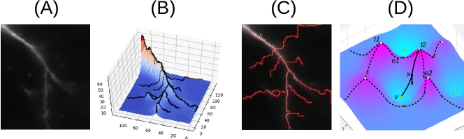
Figure 1: A practical example of DM graph reconstruction. (A) The image (downloaded from www.brainimagelibrary.org/) contains neuronal branches that we aim to reconstruct. (B) View the image as a density function, we show the graph of this function, and mountain ridges of this terrain. (C) These ridges capture potential neuronal branches in the image in (A). (D) Gradient and the integral line passing $x$. Dashed curves are union of unstable 1-manifolds.

Roughly speaking, given $\rho$, the gradient vector at $x\in{\Omega}$, $\nabla\rho(x)=-[\frac{\partial\rho}{\partial{\mathsf{x}}_{1}}(x),\ldots,\frac{\partial\rho}{\partial{\mathsf{x}}_{d}}(x)]^{T}$, indicates the steepest descending direction of $\rho$ at $x$. See Figure 1 (D). Critical points of $\rho$ are points whose gradient vector vanishes. For a smooth function on $d$-D domain, non-degenerate critical points include minima, maxima, and $d$-$1$ types of saddle points. An integral line is intuitively the flow-line traced out by following the gradient direction at every point. Flow-lines (integral lines) start and end (in the limit) at critical points. The unstable 1-manifold of a saddle (of index $d$-$1$) is the union of flow-lines starting at some maximum and ending at this saddle. Intuitively, unstable 1-manifolds connect mountain peaks to saddles to peaks, separating different valleys (around minima), and thus can be used to capture mountain ridges.

Hence one can compute the union of unstable 1-manifolds of $\rho$ as its graph skeleton. Furthermore, the density map $\rho$ may be noisy. To denoise the graph skeleton, previous approaches use persistent homology to keep only unstable 1-manifolds corresponding to "important" saddles.

Algorithm in the discrete setting.

In the discrete setting imagine $K$ is the 2-skeleton of a domain $\Omega$ of interest, $\rho$ is a density function defined on $\Omega$ but is only accessible at vertices $V(K)$ of $K$, i.e., $\rho:V(K)\to{\mathbb{R}}$. Algorithm firstDM-graph($K,\rho:V(K)\to{\mathbb{R}},\delta$) will output a graph consisting of edges of $K$ capturing a graph skeleton of the density field $\rho$ by the following three steps:

• (Step 1): Compute persistence pairing $\mathcal{P}$ induced by the lower-star filtration w.r.t. -$\rho$.

  Specifically, we use $f=-\rho$ as it is easier to algorithmicly compute the discrete analog of "valley ridges" using discrete Morse theory than "mountain ridges" – The valley ridges are the stable 1-manifolds (vertex-edge V-paths) for critical edges, and thus only 2-skeleton of input complex $K$ is needed. To compute the importance of critical points in the simplicial setting when we are given $f:V(K)\to{\mathbb{R}}$, we use the standard lower-star filtration to simulate the so-called sublevel-set filtration in the smooth case. In particular, given $f:V(K)\to{\mathbb{R}}$, let $v_{1}\ldots v_{n}$ be the set of vertices in $K$ sorted in non-decreasing order of $f$ values. Given any vertex $v_{i}\in V(K)$, its lower-star ${\mathsf{lowSt}}(v_{i})$ consists of the set of simplices incident on $v_{i}$ spanned by only vertices from $V_{i}:=\{v_{1},\ldots,v_{i}\}$. The lower-star filtration w.r.t. $f$ is the following:

  $${\widehat{K}}_{1}\subset{\widehat{K}}_{2}\subset\cdots{\widehat{K}}_{n}=K;~{}~{}~{}\text{where}~{}K_{i}=K_{i-1}\cup{\mathsf{lowSt}}(v_{i}).$$ (2)

  Equivalently, we can think that this filtration is induced by a simplex-wise function $\hat{f}:K\to{\mathbb{R}}$ where $\hat{f}(\sigma)=\max_{\text{vertex}~{}v~{}\text{of}~{}\sigma}f(v)$.

• (Step 2): Initialize vector field $M(K)$ to be the trivial one where all simplices are critical. Then in order of increasing persistence, for each pair $(\sigma,\tau)\in\mathcal{P}$ with ${\mathrm{pers}}(\sigma,\tau)\leq\delta$, perform discrete Morse cancellation and update $M(K)$ if possible. Intuitively, this is to simplify and remove "not-important" critical points.

• (Step 3): Output the graph $G_{\delta}=\bigcup_{e\in K,{\mathrm{pers}}(e)>\delta}\{$ stable 1-manifold of $e\}$.

  In particular, we only consider critical edges that are "important" (i.e., ${\mathrm{pers}}>\delta$). Then we trace the valley ridges (stable 1-manifolds) connecting them to minima. These minima - which have persistence greater than $\delta$ - are the topographically prominent peaks of $\rho$.

Simplified algorithm.

It turns out that algorithm firstDM-graph() can be significantly simplified [15]. In particular, one does not need to explicitly maintain any discrete Morse gradient vector field at all. See Algorithm DM-graph() below.

Input: Triangulation $K$, density function $\rho:V(K)\to{\mathbb{R}}$, persistence threshold $\delta$

Output: a graph skeleton $G_{\delta}$

(Step 1) Compute persistence pairing $\mathcal{P}$ induced by the lower star filtration w.r.t. -$\rho$,

(Step 2) Set ${\mathcal{T}}_{\delta}:=\{e\in E\mid e$ is negative and ${\mathrm{pers}}(e)\leq\delta\}$

 For each component (tree) $T$ in ${\mathcal{T}}_{\delta}$, set its root to be $r(T):=\mathrm{argmin}_{v\in T}$ -$\rho(v)$.

(Step 3) Let $\pi_{T}(x,y)$ be the tree path from $x$ to $y$ in a tree $T$. Output:

$$G_{\delta}=\bigcup_{e=(u,v),{\mathrm{pers}}(e)>\delta}\{e\cup\pi_{T_{i_{1}}}(u,r(T_{i_{1}}))\cup\pi_{T_{i_{2}}}(v,r(T_{i_{2}}))\mid u\in T_{i_{1}},v\in T_{i_{2}}~{}\text{in}~{}{\mathcal{T}}_{\delta}\}.$$ (3)

Algorithm 1 DM-graph($K,\rho,\delta$)

In particular, in (Step 3) above, we only consider critical edges with ${\mathrm{pers}}>\delta$, and their stable 1-manifolds turn out to be the union of tree paths as specified in Eqn (3). Note that (Step 2, 3) can be implemented in time linear to the number of vertices and edges in $K$.

3 Generalized Algorithm and Optimality

Now suppose instead of a triangulation of a $d$-D domain $\Omega$, we have an arbitrary simplicial complex $K$ – our algorithm only needs its 2-skeleton $K=(V,E,T)$. Suppose further that there is a simplex-wise function ${\widehat{\rho}}:K\to{\mathbb{R}}$. Let ${\Pi}_{\widehat{\rho}}:=\langle\sigma_{1},\ldots,\sigma_{N}\rangle$ be an ordered sequence of simplicies of $K$ that is consistent with ${\widehat{\rho}}$ (see the end of Section 2.1), and let ${\mathcal{F}}_{\widehat{\rho}}$ be the simplex-wise filtration of $K$ induced by this order ${\Pi}_{\widehat{\rho}}$. (We will describe in Section 5 how to set up this filtration for graph skeletonization from PCDs.) We now generalize algorithm DM-graph() to the following extDM-graph(), where essentially, only (Step 1) differs by taking an arbitrary simplex-wise filtration ${\mathcal{F}}_{\widehat{\rho}}$, which we state in Algorithm 2 for clarity.

Input: Arbitrary simplex-wise filtration ${\mathcal{F}}_{\widehat{\rho}}$ of a simplicial complex $K=(V,E,T)$, threshold $\delta$

Output: A reconstructed graph $G_{\delta}$

(Step 1) Compute persistence pairings w.r.t. ${\mathcal{F}}_{\widehat{\rho}}$

(Step 2) + (Step 3): same as in alg. DM-graph

Algorithm 2 extDM-graph($K,{\mathcal{F}}_{\widehat{\rho}},\delta$)

It is easy to verify that the original DM-graph($K,\rho,\delta)$ algorithm is a special case of the above algorithm, where we set ${\mathcal{F}}_{\widehat{\rho}}$ in extDM-graph($K,{\mathcal{F}}_{\widehat{\rho}},\delta$) to be the lower-star filtration induced by the vertexwise function $\rho^{\prime}=-\rho:V(K)\to{\mathbb{R}}$; specifically, for any simplex $\sigma\in K$, set ${\widehat{\rho}}(\sigma):=\max_{v\in\sigma}-\rho(v)$. The difference between our extDM-graph() algorithm and the original algorithm is rather minor. However, we will see that this change of perspective (from density-function based view to arbitrary filtration-based view) significantly broadens the applicability of this algorithm. In particular, in Section 5 we will show how this generalized algorithm can be combined with weighted Rips sparsification strategy to reconstruct a hidden graph skeleton of high-dimensional points data. But first, in what follows, we provide some characterization of the graph skeleton output by extDM-graph. Specifically, we show that the output of extDM-graph() contains the so-called lex-optimal cycle basis of $K$ w.r.t. important 1D homological features in ${\mathrm{dgm}}_{1}{\mathcal{F}}_{\widehat{\rho}}$. To make this statement more precise, we first introduce some notations, following [13, 17, 39]. Intuitively, a $1$-cycle is a collection of edges forming one or multiple closed loops; and a $d$-cycle is a $d$-D analog of it.

Definition 3.1 (Persistent cycles [17]).

Let ${\mathcal{F}}$ be a simplexwise filtration of $K$ induced by the ordered sequence of simplices $\sigma_{1},\ldots,\sigma_{N}$, and ${\mathrm{dgm}}_{q}{\mathcal{F}}$ its resulting $q$-th persistence diagram. Given a point ${\mathsf{p}}=[b,d]\in{\mathrm{dgm}}_{q}{\mathcal{F}}$, a $q$-cycle $\gamma$ is a persistent $q$-cycle w.r.t. ${\mathsf{p}}$ if (i) if $d\neq\infty$, $\gamma$ is a cycle in $K_{b}$ containing $\sigma_{b}$, and $\gamma$ is not a boundary in $K_{d-1}$ but becomes a boundary in $K_{d}$; and (ii) otherwise if $d=\infty$, then $\gamma$ is a cycle in $K_{b}$ containing $\sigma_{b}$.

Given a subset $D=\{{\mathsf{p}}_{1},\ldots,{\mathsf{p}}_{r}\}\subseteq{\mathrm{dgm}}_{q}{\mathcal{F}}$ with $r=|D|$, we say that a set of cycles $\{\gamma_{1},\ldots,\gamma_{r}\}$ form a persistent cycle-basis for $D$ if $\gamma_{i}$ is a persistence cycle w.r.t. ${\mathsf{p}}_{i}$ for all $i\in[1,r]$.

Roughly speaking, a persistent cycle $\gamma$ w.r.t. a persistence point ${\mathsf{p}}=[b,d]$ is created at $b$ and killed at $d$, and can be thought of a representative of the homological feature captured by point ${\mathsf{p}}\in{\mathrm{dgm}}{\mathcal{F}}$. A persistent cycle basis w.r.t. $D\subset{\mathrm{dgm}}{\mathcal{F}}$ corresponds to representative cycles captured by points in $D$. More specifically, given a cycle $\gamma$, let $[\gamma]_{K_{i}}$ denote the homology class of $\gamma$ in complex $K_{i}$. The following result from [17] intuitively says that a persistence cycle-basis for ${\mathrm{dgm}}_{q}{\mathcal{F}}$ essentially generates the interval decomposition of persistence module $\mathbb{P}{\mathcal{F}}$.

Claim 3.2 ([17]).

Let $\{\gamma_{1},\ldots,\gamma_{g}\}$ be a persistence cycle-basis for ${\mathrm{dgm}}_{q}{\mathcal{F}}=\{{\mathsf{p}}_{1},\ldots,{\mathsf{p}}_{g}\}$ and $g=|{\mathrm{dgm}}_{q}{\mathcal{F}}|$. Then $\mathbb{P}{\mathcal{F}}=\bigoplus_{{\mathsf{p}}_{\ell}\in{\mathrm{dgm}}_{q}{\mathcal{F}}}\mathbb{I}^{{\mathsf{p}}_{\ell}}$, where the interval module $\mathbb{I}^{{\mathsf{p}}_{\ell}}=\{I_{i}\overset{\tiny{\nu_{i,j}}}{\longrightarrow}I_{j}\}_{i\leq j}$ is generated by $\gamma_{\ell}$ in the sense that $I_{i}=[\gamma_{\ell}]_{K_{i}}$.

Lexicographic optimal cycles are introduced in [12, 13]. We will extend them to the persistence version. Given a simplex-wise filtration ${\mathcal{F}}$ of $K$ induced by an ordering of simplices $\sigma_{1},\ldots,\sigma_{N}$, we set ${\mathsf{ind}}(\sigma)$ as the order it appears in ${\mathcal{F}}$; i.e, ${\mathsf{ind}}(\sigma_{i})=i$.

Definition 3.3 (Lexicographic order [13]).

Given two $q$-cycles $C_{1},C_{2}\in{\mathsf{C}}_{q}(K)$, we say that $C_{1}{\preceq}C_{2}$ if either (i) $C_{1}+C_{2}=0$ or (ii) otherwise, the simplex $\sigma_{max}:={\mathrm{argmax}}_{\sigma\in C_{1}+C_{2}}{\mathsf{ind}}(\sigma)$ is from $C_{2}$. If (ii) holds, we say that $C_{1}{\prec}C_{2}$, i.e., $C_{1}$ is smaller than $C_{2}$ in lexicographic order. Intuitively, $C_{1}{\preceq}C_{2}$ if simplices in $C_{1}$ comes "earlier" than $C_{2}$ in the filtration order.

Definition 3.4 (Lex-optimal persistent cycles).

Given a persistence point ${\mathsf{p}}=[b,d]\in{\mathrm{dgm}}_{q}{\mathcal{F}}$, a $q$-cycle $\gamma$ is a lexicographic-optimal (lex-opt for short) persistent cycle w.r.t. ${\mathsf{p}}$ if (i) $\gamma$ is a persistent cycle w.r.t. ${\mathsf{p}}$; and (ii) among all persistence cycles w.r.t. ${\mathsf{p}}$, $\gamma$ has the smallest lexicographic order. We say that $\Gamma=\{\gamma_{1},\ldots,\gamma_{r}\}$ forms a lex-optimal persistent cycle basis for a multiset $D=\{{\mathsf{p}}_{1},\ldots,{\mathsf{p}}_{r}\}\subseteq{\mathrm{dgm}}_{q}{\mathcal{F}}$ if $\gamma_{i}$ is a lex-optimal persistence cycle w.r.t ${\mathsf{p}}_{i}$ for all $i\in[1,r]$.

Given a $q$-th persistence diagram ${\mathrm{dgm}}_{q}{\mathcal{F}}$ and a threshold $\delta$, let ${\mathrm{dgm}}_{q}{\mathcal{F}}(\delta)\subseteq{\mathrm{dgm}}_{q}{\mathcal{F}}$ denote the subset of points in ${\mathrm{dgm}}_{q}{\mathcal{F}}$ whose persistence is larger than $\delta$ (intuitively, these corresond to important features). Our first main result is the following theorem.

Theorem 3.5.

(i) $G_{\delta}$ as constructed w.r.t. a simplex-wise filtration ${\mathcal{F}}_{\rho}$ contains a lex-optimal persistence cycle basis for ${\mathrm{dgm}}_{1}{\mathcal{F}}_{\rho}(\delta)$, and (ii) the first Betti number of $G_{\delta}$ equals $|{\mathrm{dgm}}_{1}{\mathcal{F}}_{\rho}(\delta)|$.

The above theorem suggests that the output graph $G_{\delta}$ by our algorithm extDM-graph() contains the "best" loops whose homology classes have large persistence and whose edges come as early as possible in the filtration. In particular, imagine that important edges or more faithful edges come early in the filtration, then the output graph contains those loops with large persistence ($>\delta$) and formed by more faithful edges whenever possible. In the graph reconstruction from PCDs application in the next section, intuitively, if edges from high-density region come into the filtration first, then the resulting output graph will use such edges whenever possible. See Figure 4 (A) to (D).

4 Proof of Theorem 3.5

We assume that $K$ is connected. If it is not, then we will perform the following arguments to each connected component of $K$. Now recall that ${\mathcal{T}}_{\delta}:=\{e\in E\mid e~{}\text{is negative and}~{}{\mathrm{pers}}(e)\leq\delta\}$ consists of all negative edges with persistence at most $\delta$ (from (Step 2) of algorithm extDM-graph in the main paper). It is shown in [15] that ${\mathcal{T}}_{\delta}$ consists of a set of trees. Set

$$E^{+}_{\delta} :=\{e\in E\mid e~{}\text{is positive and}~{}{\mathrm{pers}}(e)>\delta\},~{}\text{and}~{}$$

$$E^{-}_{\delta} :=\{e\in E\mid e~{}\text{is negative and}~{}{\mathrm{pers}}(e)>\delta\}.$$

Set ${\widehat{G}}_{\delta}={\mathcal{T}}_{\delta}\bigcup G_{\delta}$, where $G_{\delta}$ is the output of algorithm extDM-graph. Furthermore, by construction, $G_{\delta}$ consists of edges in $E^{-}_{\delta}\cup E^{+}_{\delta}$ together with a set of tree paths in ${\mathcal{T}}$ (recall Eqn (3) in Algorithm 1, which is the same as the construction for algorithm extDM-graph). It follows that

$${\widehat{G}}_{\delta} ={\mathcal{T}}_{\delta}\bigcup G_{\delta}={\mathcal{T}}_{\delta}\bigcup E^{-}_{\delta}\bigcup E^{+}_{\delta}.$$ (4)

We prove Theorem 3.5 in two steps, laid out in the following two lemmas.

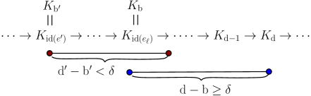
(a)	(b)

Figure 2: (a) The solid red curve is $G_{\delta}$, while dashed trees are components in ${\widehat{G}}_{\delta}\setminus G_{\delta}$. The closure of each component $C_{i}$ connects to $G_{\delta}$ at one point $w_{i}$, and thus its closure can deformation retracts to $w_{i}\in G_{\delta}$. (b) As ${\mathrm{pers}}(e^{\prime})={\mathsf{d}}^{\prime}-{\mathsf{b}}^{\prime}\leq\delta$, and ${\mathrm{pers}}({\mathrm{e}}_{\ell})={\mathsf{d}}-{\mathsf{b}}>\delta$, and ${\mathsf{b}}^{\prime}(={\mathsf{ind}}(e^{\prime}))\leq{\mathsf{b}}$, it then follows that the persistent cycle $C^{\prime}=\pi(u,v)+e^{\prime}$ must become a boundary in the simplicial complex $K_{{\mathsf{d}}-1}$, which in turn leads to that $[\gamma^{\prime}]=[\gamma^{*}]$ in $K_{{\mathsf{d}}-1}$.

Lemma 4.1.

Statements (i) and (ii) in Theorem 3.5 holds for ${\widehat{G}}_{\delta}$. That is: (i’) ${\widehat{G}}_{\delta}$ constructed w.r.t. a simplex-wise filtration ${\mathcal{F}}_{\rho}$ contains a lex-optimal persistence cycle basis for ${\mathrm{dgm}}_{1}{\mathcal{F}}_{\rho}(\delta)$, and (ii’) the first Betti number of ${\widehat{G}}_{\delta}$ equals $|{\mathrm{dgm}}_{1}{\mathcal{F}}_{\rho}(\delta)|$.

Lemma 4.2.

${\widehat{G}}_{\delta}$ deformation contracts to $G_{\delta}$.

Our theorem then follows from these two lemmas. Specifically, we will use the graph ${\widehat{G}}_{\delta}$ as a proxy: Lemma 4.1 states that the desired results hold for ${\widehat{G}}_{\delta}$. Lemma 4.2 then relates ${\widehat{G}}_{\delta}$ to $G_{\delta}$. In particular, as both ${\widehat{G}}_{\delta}$ and $G_{\delta}$ are graphs, this lemma implies that any simple cycle in ${\widehat{G}}_{\delta}$ must be present in $G_{\delta}$ as well. Theorem 3.5 then follows. What remains is to prove these two lemmas, which we present in the two subsections that follow.

4.1 Proof of Lemma 4.1

Let ${\mathrm{dgm}}_{1}{\mathcal{F}}_{\rho}(\delta)=\{{\mathsf{p}}_{1},\ldots,{\mathsf{p}}_{g}\}$. By the definition of positive and negative edges, we know:

• (C1). ${\widehat{{\mathcal{T}}}}={\mathcal{T}}_{\delta}\cup E^{-}$ is a spanning tree of $K$.

• (C2). By the definition of positive edges, $E^{+}_{\delta}$ contains exactly those edges whose addition create the persistence points in ${\mathrm{dgm}}_{1}{\mathcal{F}}_{\rho}(\delta)$. In other words, $g=|E^{+}_{\delta}|$ and we can order edges in $E^{+}_{\delta}=\{{\mathrm{e}}_{1},\ldots,{\mathrm{e}}_{g}\}$ so that for any $\ell\in[1,g]$, ${\mathsf{p}}_{\ell}=[{\mathsf{ind}}({\mathrm{e}}_{\ell}),d_{\ell}]$: i.e, the birth-time of ${\mathsf{p}}_{\ell}$ corresponds to the insertion of edge ${\mathrm{e}}_{\ell}$ in the simplicial complex $K_{{\mathsf{ind}}({\mathrm{e}}_{\ell})}$.

Furthermore, the addition of each positive edge ${\mathrm{e}}_{\ell}\in E^{+}_{\delta}$ creates a cycle in the spanning tree ${\widehat{{\mathcal{T}}}}$ (as ${\mathrm{e}}_{\ell}$ is not a tree edge), As ${\widehat{G}}_{\delta}={\widehat{{\mathcal{T}}}}\cup E^{+}$, we thus have $\beta_{1}({\widehat{G}}_{\delta}):=rank({\mathsf{H}}_{1}({\widehat{G}}_{\delta}))$ is the same as $g=|{\mathrm{dgm}}_{1}{\mathcal{F}}_{\rho}(\delta)|$. This proves part (ii’) in Lemma 4.1 for the graph ${\widehat{G}}_{\delta}$.

We now prove part (i’) of Lemma 4.1. Consider any ${\mathrm{e}}_{\ell}\in E^{+}_{\delta}$, and let $\gamma^{*}$ denote a lex-opt persistent cycle of the corresponding persistence point ${\mathsf{p}}_{\ell}=[{\mathsf{b}},{\mathsf{d}}]$ (where ${\mathsf{b}}={\mathsf{ind}}({\mathrm{e}}_{\ell})$). By Definitions 3.1 and 3.3 in the main paper, $\gamma^{*}$ necessarily contains ${\mathrm{e}}_{\ell}$, and all other edges in $\gamma^{*}$ have an index smaller than ${\mathsf{ind}}({\mathrm{e}}_{\ell})$. We will next prove that $\gamma^{*}$ is in ${\widehat{G}}_{\delta}$, that is, treating a cycle (under $\mathbb{Z}_{2}$ coefficients) as a set, $\gamma^{*}\subseteq{\widehat{G}}_{\delta}$.

In particular, take any edge $e^{\prime}\in\gamma^{*}$ with $e^{\prime}\neq{\mathrm{e}}_{\ell}$, we will show that $e^{\prime}\in{\widehat{G}}_{\delta}$.

• If $e^{\prime}$ is negative, then this is trivially true as $e^{\prime}\in{\widehat{{\mathcal{T}}}}\subseteq{\widehat{G}}_{\delta}$.

• If $e^{\prime}$ is positive but with persistence ${\mathrm{pers}}(e^{\prime})>\delta$, then it is also true as $e^{\prime}\in E^{+}_{\delta}\subseteq{\widehat{G}}_{\delta}$.

• So what remains is the case when $e^{\prime}=(u,v)$ is positive but with ${\mathrm{pers}}(e^{\prime})\leq\delta$. However, we will show that this case cannot happen, which implies that $e^{\prime}\in{\widehat{G}}_{\delta}$.

  Assume this case happens for edge $e^{\prime}$. Then let $C_{e^{\prime}}(=\pi(u,v)+e^{\prime})\subset K_{{\mathsf{ind}}(e^{\prime})}$ be a persistent cycle w.r.t. the persistence point $[{\mathsf{b}}^{\prime}={\mathsf{ind}}(e^{\prime}),{\mathsf{d}}^{\prime}]$ generated by $e^{\prime}$. First, as the path (1-chain) $\pi(u,v)$ is contained in $K_{{\mathsf{ind}}(e^{\prime})}$, all edges in $\pi(u,v)$ have an index less than that of $e^{\prime}$. This means that the cycle $\gamma^{\prime}=\gamma^{*}-e^{\prime}+\pi(u,v)$ is necessarily smaller than $\gamma^{*}$ in lexicographic order. We now claim that $\gamma^{\prime}$ is also a persistent cycle w.r.t. the persistence point ${\mathsf{p}}_{\ell}=[{\mathsf{b}},{\mathsf{d}}]$ corresponding to the positive edge ${\mathrm{e}}_{\ell}$.

  Indeed, as $\gamma^{*}$ is a persistent cycle w.r.t. ${\mathsf{p}}_{\ell}$, we know that ${\mathsf{ind}}(e^{\prime})<{\mathsf{ind}}({\mathrm{e}}_{\ell})={\mathsf{b}}$. Recall that the persistence point corresponds to the positive edge $e^{\prime}$ is $[{\mathsf{b}}^{\prime}={\mathsf{ind}}(e^{\prime}),{\mathsf{d}}^{\prime}]$. As ${\mathrm{pers}}({\mathrm{e}}_{\ell})=\rho({\mathsf{d}})-\rho({\mathsf{b}})>\delta$ while ${\mathrm{pers}}(e^{\prime})=\rho({\mathsf{d}}^{\prime})-\rho({\mathsf{b}}^{\prime})\leq\delta$, it then follows that ${\mathsf{d}}^{\prime}<{\mathsf{d}}$. (See Figure 2 (b) for illustrations of these notations.) Hence we know that it is necessary that the cycle $\pi(u,v)+e^{\prime}$ becomes boundary in $K_{{\mathsf{d}}-1}$. In other words, in $K_{{\mathsf{d}}-1}$, the two cycles $\gamma^{*}$ and $\gamma^{\prime}$ are homologous. It is then easy to verify that $\gamma^{\prime}$ must be a persistent cycle for ${\mathsf{p}}_{\ell}$ as well.

  Since $\gamma^{\prime}$ is also a persistent cycle for ${\mathsf{p}}_{\ell}$ and is lexicographically smaller than $\gamma^{*}$, this contradicts our assumption that $\gamma^{*}$ is a lex-opt persistent cycle for ${\mathsf{p}}_{\ell}$. Hence no positive edge $e^{\prime}\in\gamma^{*}$ with ${\mathrm{pers}}(e^{\prime})<\delta$ can be in $\gamma^{*}$.

By the above case analysis, any edge $e^{\prime}\in\gamma^{*}$ must be in ${\widehat{G}}_{\delta}$. It then follows that $\gamma^{*}\subseteq{\widehat{G}}_{\delta}$. As this argument holds for any edge in $E^{+}_{\delta}$, we thus have proven (i’). This finishes the proof of Lemma 4.1.

4.2 Proof of Lemma 4.2

First, by construction of ${\widehat{G}}_{\delta}$ (Eqn (4)), we have that $G_{\delta}\subseteq{\widehat{G}}_{\delta}$, and all edges in ${\widehat{G}}_{\delta}\setminus G_{\delta}$ must come from ${\mathcal{T}}_{\delta}$. Now recall ${\widehat{{\mathcal{T}}}}={\mathcal{T}}_{\delta}\bigcup E^{-}$, which is a spanning tree of $K$. Given an arbitrary tree $T$ and two nodes $u,v\in T$, let $\pi_{T}(u,v)$ denote the unique tree path from $u$ to $v$ in $T$. We have the following simple claim.

Claim 4.3.

Given any rooted tree $T$ with root $r(T)$ and two nodes $u,v\in T$, we have that $\pi_{T}(u,v)\subseteq\pi_{T}(u,r(T))\cup\pi_{T}(v,r(T))$.

Proof.

If $u$ and $v$ have ancestor / descendent relation, say $u$ is ancestor of $v$, then it is clear that $\pi_{T}(u,v)\subseteq\pi_{T}(v,r(T))$, and the claim then follows. Otherwise, let $w$ be the common ancestor of $u$ and $v$. It can again be verified that in this case, $\pi_{T}(u,w)\subseteq\pi_{T}(u,r(T))$, $\pi_{T}(v,w)\subseteq\pi_{T}(v,r(T))$, while $\pi_{T}(u,v)=\pi_{T}(u,w)\circ\pi_{T}(w,v)$. The claim thus follows. ∎

${\mathcal{T}}_{\delta}$ is a spanning forest of vertex set $V$. Given any vertex $v\in V$, suppose it is in the tree $T\in{\mathcal{T}}_{\delta}$. We denote ${path_{{\mathcal{T}}_{\delta}}}(v):=\pi_{T}(v,r(T))$ to be the path from $v$ to the root $r(T)$ of $T$. Recall that $G_{\delta}$ is constructed by, for any edge $e=(u,v)\in E_{\delta}^{-}\cup E_{\delta}^{+}$, adding $e\cup{path_{{\mathcal{T}}_{\delta}}}(u)\cup{path_{{\mathcal{T}}_{\delta}}}(v)$ into $G_{\delta}$.

Lemma 4.4.

For each edge ${\mathrm{e}}=(u,v)\in E^{+}_{\delta}$, set $\gamma=e\cup\pi_{{\widehat{{\mathcal{T}}}}}(u,v)$. Then the cycle $\gamma$ must be contained in $G_{\delta}$.

Proof.

Consider the path $\pi=\pi_{\widehat{{\mathcal{T}}}}(u,v)$: it will be broken into $k\geq 0$ maximally connected pieces from ${\mathcal{T}}_{\delta}$, connected by edges in $E^{-}\cup E^{+}$. If $k=0$, we are done, because this means that $u,v$ are contained in the same tree $T$ in ${\mathcal{T}}$, and it then follows from Claim 4.3 that

$$\pi=\pi_{T}(u,v)\subseteq{path_{{\mathcal{T}}_{\delta}}}(u)\cup{path_{{\mathcal{T}}_{\delta}}}(v)\subseteq G_{\delta}.$$

(a)	(b)	(c)

Figure 3: (a) The path $\pi=\pi(u,v)$ is broken into $k+1$ pieces, each of which (blue subcurves) is a maximal connected component in $\pi\cap{\mathcal{T}}_{\delta}$, while the connecting edges (red edges $(v_{i},u_{i})$’s) must come from $E_{\delta}^{-}\cup E_{\delta}^{+}$. (b) The solid red path is the tree path $\pi=\pi_{T}(u,w)$ connecting $u$ and $w$ in the tree $T$ from the spanning forest ${\mathcal{T}}_{\delta}$. The root of $T$ is $r(T)$. (c) The solid red curve is $G_{\delta}$, while dashed trees are components in ${\widehat{G}}_{\delta}\setminus G_{\delta}$. The closure of each $C_{i}$ connects to $G_{\delta}$ at one point $w_{i}$, and thus its closure can deformation retract to $w_{i}$.

So assume that $k>0$, and the edges connecting these pieces are $e_{1}=(v_{1},u_{1}),\ldots,e_{k}=(v_{k},u_{k})$ from $u$ to $v$ along $\pi$; see Figure 3 (a). Obviously, for each $i\in[1,k]$, $e_{i}\notin{\mathcal{T}}_{\delta}$ and $e_{i}\in E_{\delta}^{-}\cup E_{\delta}^{+}$. Set $u_{0}=u$ and $v_{k+1}=v$. It then follows that for any $i\in[0,k]$, $u_{i}$ is connected to $v_{i+1}$ within some tree, say $T\in{\mathcal{T}}_{\delta}$. By Claim 4.3 that the portion of $\pi$ from $u_{i}$ to $v_{i+1}$ must be contained in $path(u_{i})\cup path(v_{i+1})$. Applying this for all $i\in[0,k]$, it follows that

$$\pi\subseteq\big{(}\bigcup_{i\in[0,k]}(path(u_{i})\cup path(v_{i+1})\big{)}~{}\bigcup~{}\big{(}e_{1}\cup e_{2}\cdots\cup e_{k}\big{)}$$

$$=\big{(}path(u)\cup path(v)\big{)}~{}\bigcup~{}\big{(}e_{1}\cup path(v_{1})\cup path(u_{1})\big{)} \bigcup\cdots\bigcup~{}\big{(}e_{k}\cup path(v_{k})\cup path(u_{k})\big{)}.$$

As all edges $e_{1},\ldots e_{k}$ and $e$ are all in $E^{-}\cup E^{+}$, it then follows that $\pi\subseteq G_{\delta}$ and thus $\gamma=e\cup\pi\subseteq G_{\delta}$. ∎

Lemma 4.5.

$\beta_{0}(G_{\delta})=\beta_{0}({\widehat{G}}_{\delta})$, and $\beta_{1}(G_{\delta})=\beta_{1}({\widehat{G}}_{\delta})$.

Proof.

That $\beta_{1}(G_{\delta})=\beta_{1}({\widehat{G}}_{\delta})$ follows immediately from Lemma 4.4. We now prove that $G_{\delta}$ and ${\widehat{G}}_{\delta}$ also has the same number of connected components. Note that we have already assumed that $K$ is connected, and thus ${\widehat{G}}_{\delta}$ is connected as it contains a spanning tree ${\widehat{{\mathcal{T}}}}$ of $K$. So what remains is to show that $G_{\delta}$ is connected.

Assume $G_{\delta}$ is not connected, and let $C_{1},C_{2}$ be two components of $G_{\delta}$. Recall that $G_{\delta}$ is constructed by the union of paths $\bigcup_{e=(u,v)\in E_{\delta}^{-}\cup E_{\delta}^{+}}\big{(}e\cup{path_{{\mathcal{T}}_{\delta}}}(u)\cup{path_{{\mathcal{T}}_{\delta}}}(v)\big{)}$. Let $e_{1}\in C_{1}$ be an arbitrary edge from $C_{1}\cap(E_{\delta}^{-}\cup E_{\delta}^{+})$: Note that such an edge must exist, as otherwise $C_{1}$ will not be in $G_{\delta}$. Similarly, let $e_{2}\in C_{2}\cap(E_{\delta}^{-}\cup E_{\delta}^{+})$. Let $u$ be an endpoint of $e_{1}$ while $w$ be an edge point of $e_{2}$. We know that $u$ and $w$ are connected in ${\mathcal{T}}_{\delta}$ by path $\pi=\pi_{{\mathcal{T}}_{\delta}}(u,w)$. We now claim that this path must be in $G_{\delta}$; which contradicts with our assumption that $C_{1}$ and $C_{2}$ are two connected components of $G_{\delta}$. Hence our assumption is wrong, and $G_{\delta}$ must be connected as well, which finishes the proof of the claim.

What remains is to show that the path $\pi=\pi_{{\mathcal{T}}_{\delta}}(u,w)$ as described above must be in $G_{\delta}$. Let $T\in{\mathcal{T}}_{\delta}$ be the tree in ${\mathcal{T}}_{\delta}$ containing path $\pi$, and let $r_{T}$ be its root. We now perform a case analysis based on the location of $r_{T}$ w.r.t. $u$ and $w$. (Case 1): $u$ is an ancestor of $w$ in $T$; (case 2): $w$ is an ancestor of $u$ in $T$; and (case 3): otherwise. See Figure 3 (b) for an illustration of (case 3). We first prove that $\pi\subseteq G_{\delta}$ for (case 3). In this case, we have that ${path_{{\mathcal{T}}_{\delta}}}(u)\cup{path_{{\mathcal{T}}_{\delta}}}(w)$ is a superset of $\pi$, that is, $\pi\subseteq{path_{{\mathcal{T}}_{\delta}}}(u)\cup{path_{{\mathcal{T}}_{\delta}}}(w)$. Furthermore, since both $e_{1},e_{2}\in E^{-}_{\delta}\cup E^{+}_{\delta}$, by construction of $G_{\delta}$, ${path_{{\mathcal{T}}_{\delta}}}(u)\subseteq G_{\delta}$ and ${path_{{\mathcal{T}}_{\delta}}}(w)\subseteq G_{\delta}$. It then follows that $\pi\subseteq G_{\delta}$. Using a similar argument, one can show that $\pi\subseteq G_{\delta}$ for (case 1) and (case 2) as well.

Putting everything together, we have that $G_{\delta}$ is connected and thus $\beta_{0}(G)=\beta_{0}({\widehat{G}}_{\delta})$. This finishes the proof of the lemma. ∎

Now let $C_{1},\ldots,C_{s}$ be the components of ${\widehat{G}}_{\delta}\setminus G_{\delta}$, and for each $i\in[1,s]$, let $\overline{C}_{i}$ be the closure of $C_{i}$. We claim that $\overline{C}_{i}\setminus C_{i}$ can contain only one vertex, say $w_{i}$. See Figure 3 (c). Indeed, as ${\widehat{G}}_{\delta}\setminus G_{\delta}\subseteq{\mathcal{T}}_{\delta}$, each $\overline{C}_{i}$ is simply connected (i.e, it is a subtree of some tree in ${\mathcal{T}}_{\delta}$). Suppose $\overline{C}_{i}\setminus C_{i}$ contains at least two vertices, say $w$ and $w^{\prime}$. As $\overline{C}_{i}$ is connected, there is a path $\pi_{\overline{C}_{i}}(w,w^{\prime})$ connecting $w$ to $w^{\prime}$ in $\overline{C}_{i}$. On the other hand, as $G_{\delta}$ is connected (Lemma 4.5), there is another path $\pi_{G_{\delta}}(w,w^{\prime})$ connecting $w$ and $w^{\prime}$. This gives rise to a cycle $\gamma=\pi_{\overline{C}_{i}}(w,w^{\prime})\cup\pi_{G_{\delta}}(w,w^{\prime})$ in ${\widehat{G}}_{\delta}$, and this cycle is not in $G_{\delta}$. This however contradicts to what we just proved that $\beta_{1}(G_{\delta})=\beta_{1}({\widehat{G}}_{\delta})$. Hence this cannot happen.

Hence $\overline{C}_{i}$ can only connect to $G_{\delta}$ via one point $w_{i}$ as illustrated in Figure 3 (c). It then follows that ${\widehat{G}}_{\delta}$ deformation retracts to $G_{\delta}$ by contracting each subtree $\overline{C}_{i}$ to the point $w_{i}$. This finishes the proof of Lemma 4.2.

5 PCD Algorithm via Sparse Weighted-Rips

Given a PCD $P\subset{\mathbb{R}}^{d}$, we now wish to compute a graph skeleton of $P$. Our algorithm can be easily extended to the case where these points $P$ are not embedded but with only pairwise distances (or similarity) given.

A baseline approach.

A natural approach is to (i) build a simplicial complex $K$ from $P$ to "approximate" the space behind $P$, (ii) estimate a density function $\rho$ at $P=V(K)$, and (iii) then perform algorithm DM-graph. A reasonable choice for $K$ is the so-called Rips complex ${\mathrm{rips}}^{r}(P):=\{(p_{i_{0}},\ldots,p_{i_{k}})\mid\|p_{i_{j}}-p_{i_{j^{\prime}}}\|\leq r\}$: Intuitively, an edge $(p,q)\in{\mathrm{rips}}^{r}(P)$ if the distance between points $p,q\in P$ is at most $r$. A triangle is in ${\mathrm{rips}}^{r}(P)$ if all three edges are in, and similarly for higher-dimensional simplices. However, we only need 2-skeleton of ${\mathrm{rips}}^{r}(P)$, which we still denote by ${\mathrm{rips}}^{r}(P)$. The estimated density of a point is determined by summing the distances under a Gaussian kernel to each of its KNN for some k. We refer to this algorithm as baseline where we use the ${\mathrm{rips}}^{r}(P)$ as choice of complex $K$, that is, we perform DM-graph(${\mathrm{rips}}^{r}(P),\rho,\delta$).

Challenges with baseline.

This baseline approach faces several challenges. (C-1) It is usually hard to choose the right radius $r$ and the topology of ${\mathrm{rips}}^{r}(P)$ crucially decides the final output graph: see Figure 4, where if $r$ is too small, the shape is not yet captured by ${\mathrm{rips}}^{r}(P)$; for larger $r$, there can be spurious topological features (extra loops) in $K$ which cannot be simplified by persistence (as these loops are generated by edges with infinity persistence). There is also the issue that even if one has found a radius $r$ value such that ${\mathrm{rips}}^{r}(P)$ can provide the correct topology, the geometry of the graph skeleton computed by this baseline algorithm may lose resolution (e.g, Figure 4 (H)).

(C-2) Points may be sampled at non-uniform resolution, hence there may not exist a single good $r$ that can capture all features; see Figure 5. (C-3) Even for a moderate radius $r$, the size of Rips complex becomes large, making persistence computation very costly. (C-4) The Rips complex can be a poor approximation of the hidden space when there is background noise; see Figure 5 (F) and (H), where even though the hidden space consists of 5 independent cycles (see Section 6), with much background noise, even a small radius $r$ makes the Rips complex connect these noisy points and lose the hidden structure. Removing low-density points can help; however in general that can be challenging when the density distribution is non-uniform.

A DTM-Rips based approach.

The Rips complex is defined based on the Euclidean distance between input points, and does not handle noise or non-uniform point samples well. The distance-to-measure (DTM) distance is introduced in [9] to provide a more robust way to produce distance field for noisy points. We use the work of [5] to induce a weighted Rips complex from DTM distances, which we now describe briefly. In particular, given a set of points $(P,{\mathsf{d}}_{P})$ equipped with metric $d_{P}$ (for points $P\subset{\mathbb{R}}^{d}$, ${\mathsf{d}}_{P}$ is the Euclidean distance in ${\mathbb{R}}^{d}$). For a fixed integer parameter $k>0$, let ${\sf kNN}(p)$ denote the set of $k$-nearest neighbor of $p$ in $P$ under metric ${\mathsf{d}}_{P}$. For each $p\in P$, we set (DTM-induced) weight $w_{p}$ as $w_{p}=\sqrt{\frac{1}{k}\sum_{q\in{\mathsf{k}NN}(p)}{\mathsf{d}}_{P}^{2}(p,q)}$, and the weighted radius of $p$ at scale $\alpha$ as $r_{p}(\alpha)=\sqrt{\alpha^{2}-w_{p}^{2}}.$ Now given a simplex $\sigma=\{p_{i_{0}},\ldots,p_{i_{s}}\}$, we define ${\rho_{w}}(\sigma)$ to be

$${\rho_{w}}(\sigma)=\min\{\alpha^{\prime}\mid w_{p_{i_{j}}}\leq\alpha^{\prime},~{}\text{and}~{}{\mathsf{d}}_{P}(p_{i_{j}},p_{i_{j^{\prime}}})\leq r_{p_{i_{j}}}(\alpha^{\prime})+r_{p_{i_{j^{\prime}}}}(\alpha^{\prime}),\forall j\neq j^{\prime}\in[0,s]\}.$$

This gives an ordering of all possible simplices formed by points in $P$ (again, edges and triangles are needed), and the resulting filtration is called DTM-Rips filtration ${\mathcal{F}}_{{\rho_{w}}}$. Equivalently, consider the DTM-weighted Rips complex ${\sf wRip}^{\alpha}(P)$ at scale $r$ defined as: ${\sf wRip}^{r}(P)=\{\sigma=\{p_{i_{0}},\ldots,p_{i_{s}}\}\mid{\rho_{w}}(\sigma)\leq r\}$. The sequence of ${\sf wRip}^{r}(P)$ with increasing scales $r=[0,\infty)$ gives rise to the filtration ${\mathcal{F}}_{\rho_{w}}$. The weight $\omega_{p}$ is a certain average distance to the $k$NN of $p$ and thus intuitively an inverse density estimator (high density points have low weight). Given two points $p,q\in P$, the edge $\sigma=(p,q)$ has smaller ${\rho_{w}}(\sigma)$ if $p$ and $q$ has lower weight (thus higher density). Simplices spanned by higher density points will enter earlier into the filtration ${\mathcal{F}}_{{\rho_{w}}}$.

Incorporating data sparsification.

However, the size of weighted Rips can still be large. To this end, we deploy the sparsified version of DTM-Rips developed in [5]. The resulting filtration is denoted by sparse DTM-Rips $\widehat{{\mathcal{F}}}_{\rho_{w}}({\varepsilon})$ which uses a sparsification parameter ${\varepsilon}>0$. See [5] for details of its construction. Our final graph skeletonization algorithm for PCDs, denoted by DM-PCD($P,k,{\varepsilon},\delta$), consists of only two steps:

(Step 1). Compute the sparse DTM-Rips filtration $\widehat{{\mathcal{F}}}_{\rho_{w}}({\varepsilon})$ using parameters $k$ (to compute DTM-weights of points) and ${\varepsilon}$ (for sparsification).

(Step 2). Apply extDM-graph($K,\widehat{{\mathcal{F}}}_{\rho_{w}}({\varepsilon}),\delta$) to compute the graph skeleton of $P$, where $K$ is given implicitly as all simplices in $\widehat{{\mathcal{F}}}_{\rho_{w}}({\varepsilon})$.

Intuitively, using the DTM-weight alleviates the problem of noisy points (challenge (C-4)), using sparsification addresses the issue of size (challenge (C-3)), while using the entire sparse DTM-Rips filtration allows us to use all radii/scales (instead of a Rips complex at a fixed radius $r$ as in baseline), thereby addressing challenges (C-1) and (C-2). Also, while at a larger radius, the filtration will include edges and triangles spanned by far-away points. Theorem 3.5 guarantees that we will output those important loop features using edges that come in as early as possible, i.e., those spanned by higher density points (with smaller ${\rho_{w}}$ values) whenever possible. This allows DM-PCD to capture hidden graphs across different scales. See Figure 5.

6 Experimental Results

We compare our DM-PCD algorithm with the baseline algorithm introduced in Section 5, and with SOA graph skeletonization algorithms based on Reeb graph [23] and Mapper [35] (referred to as ReebRecon and Mapper below). (Mapper can produce higher dimensional structures beyond graph skeleton, although often 1D structures are used in practice.) We test on two synthetic point sets and three real datasets. Unless otherwise specified, we use $k=15$ and ${\varepsilon}=.99$ in our DM-PCD($P,k,{\varepsilon},\delta$); while the persistence simplification threshold $\delta$ depends on the point set at hand. For baseline, ReebRecon, and Mapper we report the results of the best parameters we find for them. In particular, a key input for the Mapper algorithm is an appropriate filter function. We tested several standard choices, including distance to base point, eccentricity, density, graph Laplacian eigenfunction and so on, and report the best results found. For all experiments, all methodologies are run on the original point cloud data, and the figures showing results of higher dimensional data display projections of the results into a lower dimensional space. Significantly more results and details are in the Appendix.

Overview.

Methods are run on five total datasets - two lower-dimensional (2-D) synthetic datasets, image patches dataset [8] (8-D), time-delay embedding of traffic sensor datasets [7] (6-D), and Coil-20 [30] (16384-D). Our experiments show that DM-PCD is able to extract the true underlying structure of all of these datasets while the other methodologies struggle with noise (image patches and traffic datasets), capturing features at different scales (synthetic and Coil-20 datasets), and having geometrically faithful outputs (synthetic datasets). Additionally, the size of the filtration used by DM-PCD is consistently smaller than that used by baseline.

Synthetic datasets.

We create two synthetic PCDs to illustrate the behavior of our DM-PCD algorithm. Circle dataset contains a noisy and non-uniform sample around a hidden circle with 2050 points. DM-PCD is able to recover a geometrically faithful hidden circle. The other methodologies, which require more parameters, also recover a hidden circle, but with a less geometrically faithful structure. Additionally, baseline requires far greater running time for comparable results. See Figure 4: the output of our method (in (C)) recovers the hidden circle. In comparison, outputs of baseline algorithm over the Rips complex ${\mathrm{rips}}^{r}(P)$ at different radius values are shown in (E) – (H). The total number of simplices involved in our sparsified DTM-Rips filtration is $368,276$. The successful baseline result (shown in Figure 4 (G)) however requires $7,708,243$ simplices, which is about 20 fold increase in size. This results in a drastic run-time difference (2.6 seconds vs. 44.8 seconds) between DM-PCD and baseline. In general, DM-PCD is more efficient than baseline because persistence is computed on a much smaller filtration (see Appendix for fully detailed timing results on all datasets). Also, in general, it is not clear which $r$ to choose for baseline, and if $r$ is too large (e.g., Figure 4 (H)), then the output graph is geometrically not faithful any more – this is because long edges are now present in the Rips complex and can appear early in the lower-star filtration in the DM-graph algorithm. In contrast, our output (in (C)) takes advantage of the lex-optimality of the algorithm (Theorem 3.5) and thus always uses "good" edges (small edges from high density regions that enter the filtration early) first. The ReebRecon approach also uses Rips complex at a fixed scale $r$ and thus has similar issues with baseline. The Mapper approach (Figure 4 (J)) correctly captures topology of the space, but misses some geometric details.

The top row of Figure 5 shows the reconstruction from a set of 300 points non-uniformly sampled from two circles (of different sizes) with background noise. DM-PCD successfully captures both circles, while other methods either fail to capture both circles, or have a topologically correct output that is less geometrically faithful than our method’s output. Our algorithm scans through all scales in the filtration and captures both loop features. In contrast, both baseline and ReebRecon can capture only one loop. Using a small radius $r$, they can capture the small loop but not the big one. To capture the large loop, they need to use a large radius $r$ (as in Figure 5 (C) and (D)), at which point the small loop is destroyed in the Rips complex. Mapper is able to capture both loops, but again some geometric details are lost (Figure 5 (E)). See more results in the Appendix.

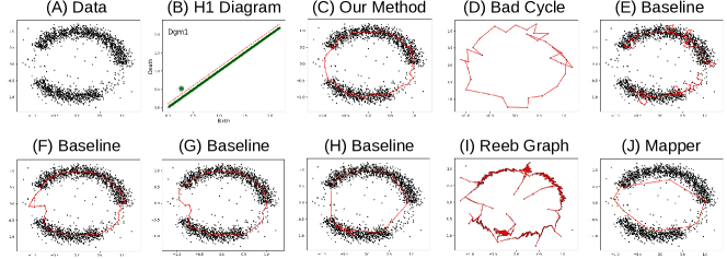
Figure 4: (A) Noisy sample of a circle. (B) 1-D persistence diagram w.r.t. our later sparse DTM-Rips filtration. Persistence points are green. Only one point (big point) ${\mathsf{p}}$ has persistence larger than some threshold $\delta$ (above the red dotted line). (C) Output of our DM-PCD method with persistence threshold $\delta=.25$, which is a lex-optimal persistent cycle w.r.t. the only high persistence point ${\mathsf{p}}$ in (B). (D) shows a "bad" persistent cycle w.r.t. the same high persistence point ${\mathsf{p}}$. In contrast, our output in (C) uses good (high density) edges whenever possible. (E) – (H) are outputs from the baseline algorithm using different radius $r$. (E) $r=0.1$: The underlying shape (circle) is not yet captured. (F) $r=0.2$: There are spurious loops that cannot be simplified via persistence. (G) $r=0.25$: The circle is recovered; however, the size of ${\mathrm{rips}}^{r}(P)$ is now 20 times that of our sparse DTM-Rips filtration. (H) $r=1.05$: The output loses geometric details. (I) is output from ReebRecon using ${\mathrm{rips}}^{r}(P)$ with radius $r=.25$ and has much noise. (J) is output from Mapper using graph Laplacian filter ($k=15$).

Image patches dataset.

The image patches dataset from [8] contains $50K$ points in $\mathbb{S}^{7}\subset{\mathbb{R}}^{8}$, each of which corresponds to a 3x3 image patch [28]. We subsample $10K$ points randomly so computationally we can experiment with Rips complexes at different radii for the baseline. DM-PCD is the only method that can extract the true underlying structure from the dataset. All other methods fail to extract any meaningful structure. The projection of points in 3D (Figure 5 (F)) is very noisy. However, the analysis of [8] shows that the underlying space has a "three-circle model", with two circles intersecting the third circle twice but not intersecting each other, thus the first Betti number of the underlying space is $5$. Our DM-PCD (shown in Figure 5 (G)) successfully recovered the same "three-circle model" (with correct $\beta_{1}=5$) directly from raw data without preprocessing, and the locations of these (outer, horizontal, and vertical) circles match those shown in [8]. Both baseline and Mapper (in Figure 5 (H) and (I)) fail to capture it. (More details in the Appendix.) Results by ReebRecon are omitted for this data set, as the algorithm does not handle background noise well and results are poor.

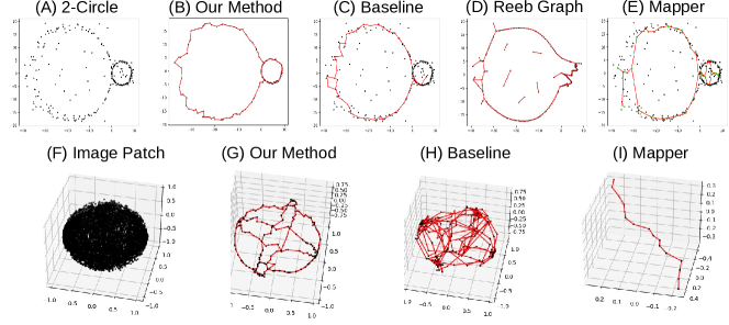
Figure 5: Top row: 2-circle data. Output of our DM-PCD method with persistence threshold $\delta=1.2$ in (B); of baseline in (C), of ReebRecon in (D), and of Mapper in (E). Using a smaller radius $r$ for baseline and ReebRecon will lose the large circle. Mapper output misses geometric details. Bottom row: image patch dataset with projection in ${\mathbb{R}}^{3}$ shown in (F). Our output with persistence threshold $\delta=.146$ in (G) captures the 3-circle model (with $\beta_{1}=5$) perfectly. For baseline in (H), further simplification will remove the main circle from the "3-circle model" while keeping all the noisy ones. Mapper (I) (base point filter) is unable to capture any of the loops.

Traffic flow dataset.

We extract two time-series from [7], which are the traffic flows at detector $\#$409529 from the time-range 10/1/2017 to 10/14/2017 and from the time-range 11/19/2017 to 12/2/2017 (including Thanksgiving). Each time-series is mapped to a PCD in ${\mathbb{R}}^{6}$ via time-delay embedding as proposed by [32], who also propose that loops in the resulting PCD can be used to detect quasi-periodic behavior in the original time-series data. We note that a normal time range has one major loop, indicating one major periodicity; while the Thanksgiving period has two: a normal one and one that indicates the traffic pattern over the holiday weekend. DM-PCD recovers these loops much better than baseline and Mapper. Results by ReebRecon are again omitted due to low quality.

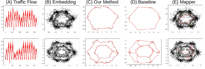
Figure 6: Top row: traffic flow for range (10/1/2017 - 10/14/2017) and bottom row is for range (11/19/2017 - 12/2/2017). (A) input time series, and (B) 2d projections of the time delay embeddings of the time-series. (C) Outputs of our DM-PCD algorithm with persistence thresholds of $\delta=50$ (top row) and $\delta=12.5$ (bottom row). (D) Outputs of the baseline approach. For the Thanksgiving period, any further simplification will destroy the outer-loop but not the cross connections. (E) Outputs of Mapper with graph Laplacian filter ($k=15$).

Coil-20 dataset.

In our final experiment, we use the Coil-20 dataset provided by [30]. More specifically, we take a subset of 17 objects - removing objects 5, 6, and 19. Objects 5 and 9 are both medicine boxes, and objects 3, 6, and 19 are toy cars, and we wanted to evaluate our method’s performance on a dataset containing unique objects. We refer to this subset as Coil-17. Following the process used by [29] to convert images to point clouds, we convert each 128 x 128 gray scale image into a 16384 dimensional vector. Hence the input is a set of 1224 points in ${\mathbb{R}}^{16384}$. Outputs of other methods can be found in the Appendix.

We visualize the data in two dimensions using UMAP dimensionality reduction with L1 metric. Presumably, each class forms a high-dimensional loopy shape. We run DM-PCD using L1 metric with $k=5$. DM-PCD is able to capture most of the individiual coils UMAP does, while providing a more correct representation of some classes than UMAP. Shown in Figure 7 is the UMAP reduction with objects uniquely colored (A), the output of our DM-PCD algorithm with a persistence threshold of 0 (B), the output of our DM-PCD algorithm with a persistence threshold of 56 (C), and the output in (C) after removing the critical edges with L1 length above a threshold of 1700 in the 16384 dimensional original space (D). The raw output contains the loops that we would expect to see based on our understanding of the data and the shapes formed in the UMAP projection. The raw output also contains many other edges, revealing more relationships both within individual classes and across multiple classes in the feature space. We remove the longer edges in order to better highlight the features of the output that capture individual objects.

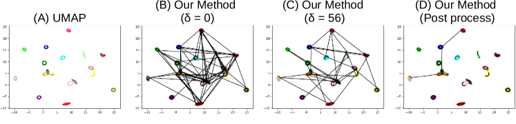
Figure 7: Coil: (A) The UMAP projection (using L1 metric) of Coil-17. (B) Output of our DM-PCD algorithm with persistence threshold $\delta=0$. (C) Output of our DM-PCD algorithm with persistence threshold $\delta=56$. (D) The output shown in (C) with critical edges of L1 length greater than 1700 removed from the output.

Taking a closer look at Figure 7 (D), there are eight objects that the DM-PCD captures in the same exact manner that the UMAP projection does. Close up pictures of these eight objects are shown in Figure 8.

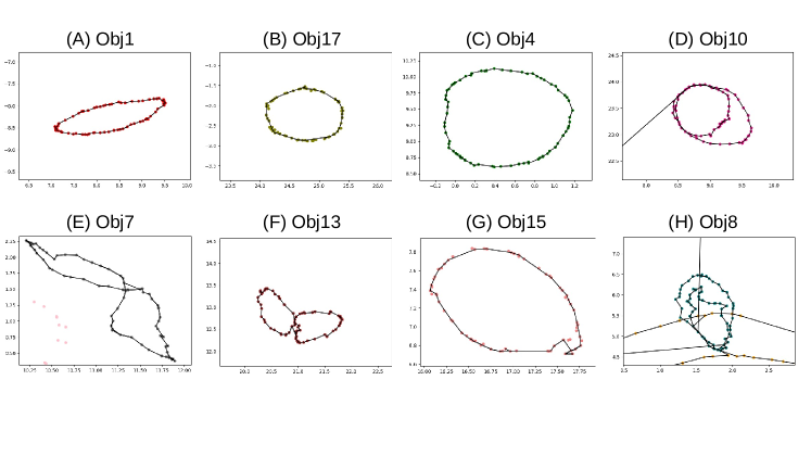
Figure 8: Coil: Zoom ins of Figure 7 (D) on the eight objects for which our DM-PCD post processed output matches the UMAP projection.

There are also four objects that both the DM-PCD output and the UMAP projection capture as loops, but the loops differ between the two methods. Close up pictures of these four objects are shown in Figure 9. Object 11 (Figure 9 (A)) is a single loop in the UMAP projection, but is actually two full loops in the DM-PCD output. A closer look (Figure 9 (B)) at images 16, 17, 54, and 55 shows two separate loops in the output. The L1 distances between these images in the 16384 dimensional original space (1069.2157046029981, 1038.6980409049952, 693.1607849029981, and 566.901973108997) for pairs (16,54), (17,55), (16,17), and (54,55) respectively) do not match the distances between the pairs in the UMAP projections. This indicates that the UMAP projection does not preserve the underlying structure of this object, and that the DM-PCD output containing two loops is correct.

A similar result is obtained for Object 14 (Figure 9 (C)), where UMAP projects a single loop and the DM-PCD output contains multiple loops. Objects 11 and 14 are symmetrical, adding further justification that multiple loops is a better skeletonization.

Object 2 (Figure 9 (D)) makes a complete loop in the DM-PCD output, but the loop looks incomplete in the UMAP projection. We ran UMAP projections on smaller subsets of Coil-20, some of which project Object 2 as a clear loop (Figure 9 (E)), whereas the DM-PCD output consistently captures Object 2 as a loop.

Object 20 (Figure 9 (F)) is captured as the same loop in both the UMAP projection and the DM-PCD output, but the DM-PCD output has an additional edge dividing the loop. The edge connects images 44 and 70, which have a L1 distance of 1329.8000237339966 in the original space. While the other edges adjacent to these nodes are much shorter, other edges that would similarly divide the loop into two are much longer. For example, the L1 distance between images 19 and 58 is 1822.1608110429997. The dividing edge in the DM-PCD output captures this difference, whereas the UMAP projection has no indication of such a difference.

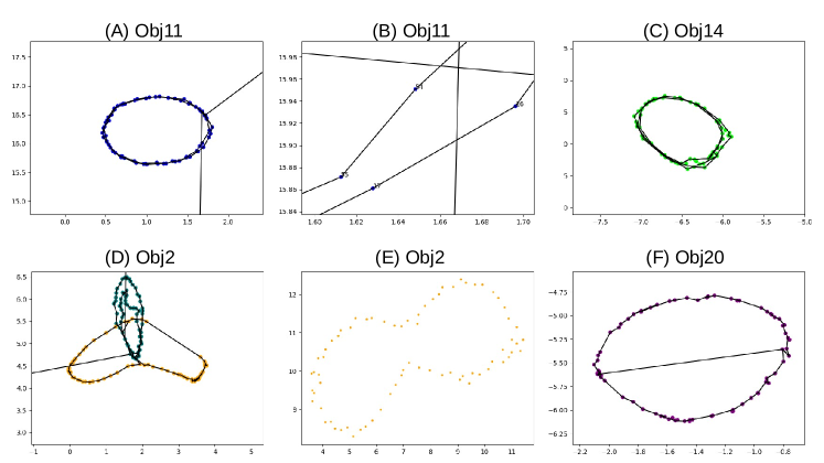
Figure 9: Coil: Zoom ins of Figure 7 (D) on the four objects for which our DM-PCD post processed output captures a different loop than the UMAP projection. (A) Object 11 - While it appears at first glance that the DM-PCD output matches the loop the UMAP projection contains, a closer look reveals (B) that the DM-PCD output actually captures two loops. (C) Object 14 - Similarly to Object 11, the DM-PCD output contains multiple loops and UMAP projection only captures one. (D) Object 2 - UMAP projection is not a complete loop, but DM-PCD produces a complete loop. (E) Object 2 - UMAP projection of only Object 2’s images - a complete loop is visible. (F) Object 20 - UMAP projection shows a single loop, while the DM-PCD output captures the same loop, but has an additional edge dividing the loop.

For the remaining five objects, it is not as clear whether or not the DM-PCD output is correct. Close ups of all five objects are shown in Figure 10. For each object, the figure shows the output at persistence thresholds $\delta=0$ (first row), $\delta=56$ (second row), and $\delta=56$ with critical edges longer than 1700 removed (third row). Object 3 (Figure 10 (A)) and Object 18 (Figure 10 (E)) are not captured as a loop in either the UMAP projection or in any DM-PCD output. The arcs appear to follow the arcs embedded in the UMAP projection. Object 9 (Figure 10 (B)) does appear as a loop in the UMAP projection, but is captured as a (double) arc by DM-PCD. Object 12 (Figure 10 (C)) is captured as a loop in UMAP, but is not in any DM-PCD output. However an arc spanning most of the loop is clearly captured. Under different parameters, DM-PCD was able to extract a loop. Object 16 (Figure 10 (D)) is captured as a loop in UMAP, and a loop is only captured by DM-PCD with persistence threshold $\delta=0$.

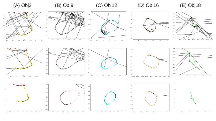
Figure 10: Coil: Zoom ins of DM-PCD outputs with persistence thresholds $\delta=0$ (first row), $\delta=56$ (second row), and $\delta=56$ with critical edges longer than 1700 removed (third row). The objects of focus are (A) Object 3, (B) Object 9, (C) Object 12, (D) Object 16, and (E) Object 18.

A final note on comparing DM-PCD to UMAP projections - the metric distortion of UMAP became apparent when viewing the DM-PCD outputs. There is metric distortion within classes - such as Object 20, where there appears to be an extra edge in the DM-PCD output because the UMAP embedding does not preserve the distances in the original space. There is also clear metric distortion in the UMAP embedding with respect to object relationships. For example, before removing critical edges with length greater than 1700, both Objects 4 and 16 have an edge that connects to Object 8. However, once the thresholding is applied, the edge connecting Objects 4 and 8 is removed and the edge connecting Objects 16 and 8 remains. This would indicate that Object 16 is closer to Object 8 than Object 4 is, but Object 4 appears closer in the UMAP embedding.

7 Concluding Remarks

We generalized the DM-graph reconstruction algorithm to arbitrary filtrations, proved that the output of this generalized algorithm is meaningful, and developed a method for graph reconstruction from high-dimensional PCDs. Empirical results demonstrate the effectiveness of our DM-PCD approach.

Time complexity is the main limitation of our approach. The time to compute persistence is a function of the size of the input filtration. While the theoretical worst case running time is cubic in this size, in practice modern implementations (such as PHAT) perform in subquadratic time (we observe near-linear growth of time w.r.t. the size of simplicial complex in our experiments). Hence reducing the size of filtration is crucial in practice. While the sparsification strategy we used in this paper helps to bring down the size of filtration, the reduction might not be significant enough for very large or more challenging datasets than what we experiment with in our paper.

In addition to running time causing potential limitations, the raw output of our DM-PCD method must be connected. As shown in Coil-20, with some post-processing we were able to capture individual objects quite easily - but the proper post-processing approach will depend on individual datasets and may not be so straight forward.

8 Data and Code Availability

Code for both our new methodology and the baseline approach is publicly available at https://github.com/lucasjmagee/PCD-Graph-Recon-DM. The repository also contains all datasets used in this manuscript.

Appendix A Further Study of Alternative Approaches

Different input triangulations for baseline  Our main experiments compare the quality of our DM-PCD method to the baseline algorithm. baseline takes an input triangulation, for which we chose the Rips complex at a fixed radius. We tested other input triangulations to highlight that the baseline approach fails regardless of the input triangulation. Results are shown in Figure 11. Even using sparse weighted Rips complex at a fixed radius large enough to capture the larger feature with less noise compared to a regular Rips complex, the points forming the smaller feature are connected by nearly a clique. Using this triangulation with any valid density function as input for the baseline algorithm results in the smaller feature being lost. It is also shown that using the weighted Rips complex without sparsification results in a similar triangulation and final output.

Different input filtrations for generalized algorithm  Our DM-PCD algorithm takes a sparse weighted Rips filtration of a point cloud dataset. However, we generalized the discrete Morse graph reconstruction algorithm to take an arbitrary filtration. To highlight the utility of the sparse weighted Rips filtration, we run the generalized discrete Morse graph reconstruction algorithm with both the regular Rips filtration and the regular weighted Rips filtration. Results are shown in Figure 12. Using the regular Rips filtration, the output captures the two features with a lot of additional noise. Trying to use persistence thresholding to remove the noise will remove the smaller feature before all noise is removed. The regular weighted Rips filtration is able to perfectly capture both features, similarly to using the sparse weighted Rips filtration. However, because the persistence computation of the filtration is a bottleneck, the sparse filtration is a superior option for our DM-PCD algorithm.

Dimensionality reduction of noisy data  For noisy datasets, such as the image patches dataset, dimensionality reduction techniques alone fail to reveal meaningful structure. Results of such techniques are shown in Figure 13. The main paper shows our DM-PCD algorithm extracts a clear three circle structure that is known to be the true underlying structure of the image patches data. However, PCA, tSNE, and UMAP projections of the image patches dataset reveal no meaningful structure (Figure 13 (A) - (C)). This is because these methods do not look to preserve metric relations. In particular, tSNE attempts to cluster data and UMAP attempts to preserve continuous structure. For cleaner data, such as Coil-20 (Figure 13 (D)), we see that UMAP is able to capture structure. However, even applying PCA and UMAP (Figure 13 (E) and (F)) to the much cleaner $X(15,30)$ subset of image patches, we see that UMAP is still unable to capture the known three circle structure of the data. Running the baseline and Mapper approaches on the PCA reduced image patches data also fails to extract the correct structure. Results are shown in Figure 14. Running baseline with a persistence threshold $\delta=2$ results in a graph where three circles appear visible (Figure 14 (B)). However, the topology is incorrect, as all circles intersect twice (the first Betti number is equal to 7). Raising the persistence threshold to 4 (Figure 14 (C)) results in an output with the correct first Betti number equal to 5, but we have clearly lost the 3 circles. Mapper fails on the PCA reduced data and the output is very similar to the output on the original data (Figure 14 (D)). This example highlights a general problem with performing dimensionality reduction then performing graph reconstruction - one needs to reduce to an appropriate dimension. Clearly it would not be possible to extract the correct graph structure from the images patches dataset if it were first reduced to 2 dimensions. It turns out that reducing to 3 dimensions is also too much, as we are unable to capture the proper (dis)connections between circles. Not having to reduce dimension, and more so not needing to know the limit for dimensionality reduction, is a huge advantage to our method.

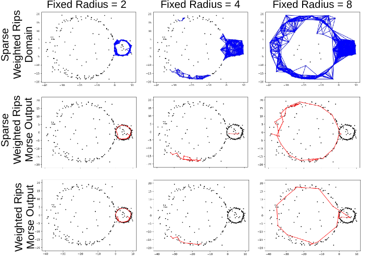
Figure 11: Sparse weighted Rips complex at fixed radii (first row) with results of baseline using sparse weighted Rips complex (second row) and full weighted Rips complex (third row). Fixed radii values of 2 (first column), 4 (second column), and 8 (third column) are shown.

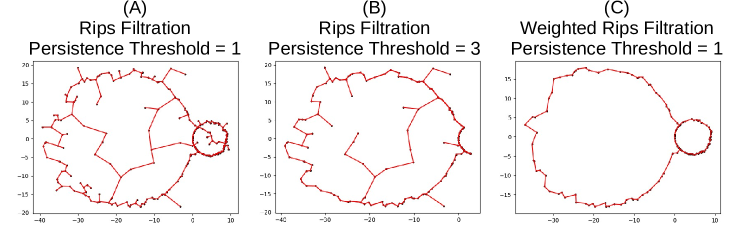
Figure 12: Results of using the generalized discrete Morse algorithm with the regular Rips filtration as input. At a lower persistence threshold (A), both features are captured with additional noise. At a higher persistence threshold (B), the smaller feature is lost while some noise remains. Using the weighted Rips filtration as input (C), the algorithm is able to recover both features with no noise.

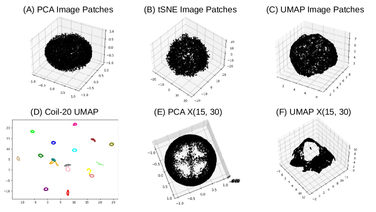
Figure 13: Outputs of various dimensionality reduction techniques (PCA, tSNE, and UMAP) performed on the 10,000 image patch subset ((A) - (C)), Coil-20 (D), and $X(15,30)$ ((E) and (F)).

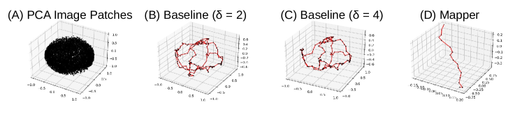
Figure 14: PCA reduction of image patches dataset (A) and outputs of baseline with persistence thresholds 2 and 4 (B and C), and Mapper (base point filter) (D) on the PCA reduced image patches dataset.

Appendix B More Details on Experiments

Comparison of methods  Our experiments compare the quality of outputs and computational efficiency of our DM-PCD method with the baseline algorithm and the state-of-the-art ReebRecon algorithm. We also compare the quality of outputs to those of the Mapper algorithm. We do not include Mapper running times in our comparisons of computational efficiency because it is significantly faster than the other algorithms.

The ReebRecon algorithm has two outputs - a contracted output, which contains only non-degree two nodes, and an augmented output, which contains edges going through every possible node in the domain. While the contracted outputs are useful for examining the topology of the output, they do a poor job of preserving the underlying geometry of the output. On the other hand, the augmented outputs are very noisy because every node is included. For this reason, the authors of the ReebRecon algorithm smooth outputs. We smooth the augmented outputs by subsampling the arcs (non-degree two paths), and then perform standard iterative smoothing on the remaining vertices. An example is shown in Figure 15. Unless otherwise noted, the ReebRecon results displayed in figures are the smoothed augmented outputs. Ultimately, the quality of the output is now dependant on the smoothing, and we note that different smoothing techniques may result in better quality outputs. However, the topology of the outputs is often incorrect, and in such cases no smoothing can make the output "correct".

The Mapper algorithm traditionally outputs a simplicial complex and was not developed to explicitly extract underlying graph structures from data. For all of our experiments, we limit the Mapper output to be a graph (1-dimensional simplicial complex). Each node in a graph outputted by Mapper represents a cluster computed within the algorithm. We assign the coordinates of a node to be the average coordinates of the cluster it represents.

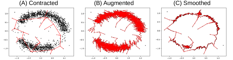
Figure 15: ReebRecon outputs on one circle dataset. The contracted output (A) and the augmented output (B) of the ReebRecon algorithm with $r=.25$. The contracted output is useful in examining the topology of the output, but does a poor job of preserving the geometry of the underlying skeleton. The augmented output better preserves the geometry but contains a lot of noise. (C) is a smoothed augmented output with less noise.

In our time comparisons, ReebRecon is much slower than both DM-PCD and baseline. While we are using an old implementation from 2011 that may not be optimized, it is known that ReebRecon is theoretically faster than both DM-PCD and baseline, which have persistence computation as a bottleneck. DM-PCD tends to be more efficient than baseline, as the sparsification in our algorithm builds a filtration that is linear in size with respect to the number of points, whereas the regular Rips complex used in baseline results in a filtration of size $O(n^{3})$, and $r$ values large enough to capture the underlying skeleton will have much bigger filtrations.

One Circle dataset.  The main paper shows that our DM-PCD algorithm is able to successfully capture the circle, and both the baseline and ReebRecon capture the circle with $r=.25$. However, the quality of output for both baseline and ReebRecon is heavily dependent on the value of $r$ - more specifically the corresponding ${\mathrm{rips}}^{r}(P)$ complex. Shown in the first row of Figure 16 is the ${\mathrm{rips}}^{r}(P)$ complex for $r$ values of .1 (A), .2 (B), .25 (C), and 1.05 (D). The second and third rows contain results of baseline and ReebRecon. All ReebRecon outputs are smoothed with no subsampling, a neighborhood radius of 2 neighbors, and 5 iterations - except for (D), where the output is a spanning tree and smoothing does not improve output quality. With an $r$ value too small (.1), the underlying skeleton is not contained in ${\mathrm{rips}}^{r}(P)$, and neither method will be able to produce a desirable output. It is not enough to select an $r$ value that results in the complex containing the underlying skeleton. For $r=.2$, the circle is captured by the ${\mathrm{rips}}^{r}(P)$ complex, but so is an additional spurious loop. Neither baseline or ReebRecon can produce an output not containing the spurious loop. For $r=1.05$, there are no additional spurious loops in the ${\mathrm{rips}}^{r}(P)$ complex, but ReebRecon produces a spanning tree and baseline, while producing a single loop, loses the geometry of the underlying skeleton.

For this dataset, $r=.25$ was an appropriate selection for both baseline and ReebRecon. However, as shown in Table 1, the size of the ${\mathrm{rips}}^{r}(P)$ complex is much bigger than the sparsified weighted Rips complex used in our DM-PCD algorithm. Complex size is particularly costly for our DM-PCD method and the baseline method because of the persistence computation. While baseline was able to produce a reasonable output at $r=.25$, it took significantly more time than our DM-PCD algorithm.

While smoothing certainly decreases the noise in the ReebRecon output, the output quality is still worse than that of both DM-PCD and baseline. We comment that a different smoothing method may result in a better quality output.

Additionally, the main paper shows that the Mapper approach is also able to successfully capture the circle. We show the ${\sf Mapper}{}$ results with a variety of filter functions in Figure 17. The graph Laplacian filter and the distance to base point filter are able to capture the circle, while the eccentricity filter and the Gaussian density filter are unable to capture the true underlying structure of the data. The heat maps of the filter functions shown in the first row of Figure 17 provide intuition on why each filters is either successfully or unsuccessfully used to extract the underlying structure with Mapper. These two filter functions will be the top choices for most of the remaining datasets.

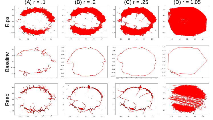
Figure 16: One circle data - ${\mathrm{rips}}^{r}(P)$ complex (first row), baseline outputs (second row), and ReebRecon outputs (third row). (A) $r=.1$ - ${\mathrm{rips}}^{r}(P)$ complex fails to capture the circle, resulting in both methods failing to capture the circle. (B) $r=.2$ - ${\mathrm{rips}}^{r}(P)$ complex now contains the circle, but also contains a spurious loop. Both the baseline output, which was generated with persistence threshold $\delta=\infty$, and the ReebRecon output must contain this spurious loop (C) $r=.25$ - ${\mathrm{rips}}^{r}(P)$ complex now contains the circle without any additional spurious loops. Both the baseline output ($\delta=\infty$) and the ReebRecon output capture the loop. (D) $r=1.05$ - ${\mathrm{rips}}^{r}(P)$ complex still contains the circle, as well as many more simplices. As a result, the baseline output has lost its nice geometry, with long edges going through high density regions, and the ReebRecon output is a spanning tree.

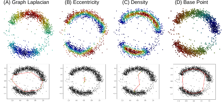
Figure 17: One circle data - Filter function values (first row) and corresponding Mapper outputs (second row) with filter functions - (A) graph Laplacian filter ($k=15$), (B) eccentricity filter, (C) Gaussian density filter, (D) distance to base point filter.

Method	Radius	$\#$ Simplices	Time (seconds)
Our Method	$\infty$	368276	2.6
Baseline	.05	33368	.1
Reeb Graph	.05	33368	.03
Baseline	.10	356925	1.1
Reeb Graph	.10	356925	2.49
Baseline	.15	1490149	5.4
Reeb Graph	.15	1490149	21.05
Baseline	.2	3869507	13.0
Reeb Graph	.2	3869507	76.46
Baseline	.25	7708243	44.8
Reeb Graph	.25	7708243	221.25
Baseline	.5	43392850	231.1
Reeb Graph	.5	43392850	3445.10

Table 1: One circle dataset: Comparison of radius used, $\#$ simplices, and running time of DM-PCD, baseline, and ReebRecon. Our algorithm has radius $\infty$ as we run on the full sparse DTM-Rips filtration.

Two Circle dataset.  The main paper shows that our DM-PCD algorithm is able to successfully capture both circles, while both baseline and ReebRecon failed to capture both circles. Again, this is because both methods are heavily dependent on the input triangulation (the ${\mathrm{rips}}^{r}(P)$ complex). This complex at various values of $r$ is shown in the first row of Figure 18, while the corresponding baseline and ReebRecon outputs are shown in the second and third rows respectively. All ReebRecon outputs are smoothed with no subsampling, a neighborhood radius of 2 neighbors, and 10 iterations. Neither result can contain the larger circle if the input triangulation itself does not contain the larger circle, so we increase values of $r$ until the complex contains the larger circle. $r=1$ is too small to capture even the smaller circle. At $r=1.5$, the complex does contain the smaller circle, and both baseline and ReebRecon are able to successfully extract the loop. However, at $r=2$ and $r=3$, the complex still does not contain the larger circle, and more noise around the smaller circle is added to the outputs. Finally, at $r=4$, the larger circle is contained within the complex. However there are two issues. Firstly, there is a spurious loop in the complex along the larger circle, so while $r=4$ is able to capture the larger circle, it is still not an appropriate value of $r$. We would need to try to find a new $r$ value that better captures the data if not for the second issue - the smaller circle is lost in both outputs - meaning an appropriate value of $r$ does not exist for either method. We can see that in the ${\mathrm{rips}}^{r}(P)$ complex at $r=4$, the points forming the smaller circle now nearly form a clique, which results in both baseline and ReebRecon outputs losing the smaller circle. We conclude that there is no value for $r$ that will result in either method capturing both circles. Running time and simplicial complex size comparisons are shown in Table 2. For radius $r=4$, we see that the number of simplices used in both baseline and ReebRecon is nearly double that of the filtration used by DM-PCD. As a result, the running times of baseline and ReebRecon are longer than that of DM-PCD.

Additionally, the main paper shows that Mapper was able to successfully capture both features of the two circle dataset. Further results for different filter functions are shown in Figure 19. Similarly to the results of the one circle dataset, Mapper was able to successfully capture both features when using either the graph Laplacian filter or distance to base point filter. Looking at the heat map for the eccentricity filter, we see that it would also appear to be an acceptable choice for this particular dataset. The output captures the larger feature and is unable to capture the smaller feature. The density filter once again fails to extract any meaningful structure from the dataset.

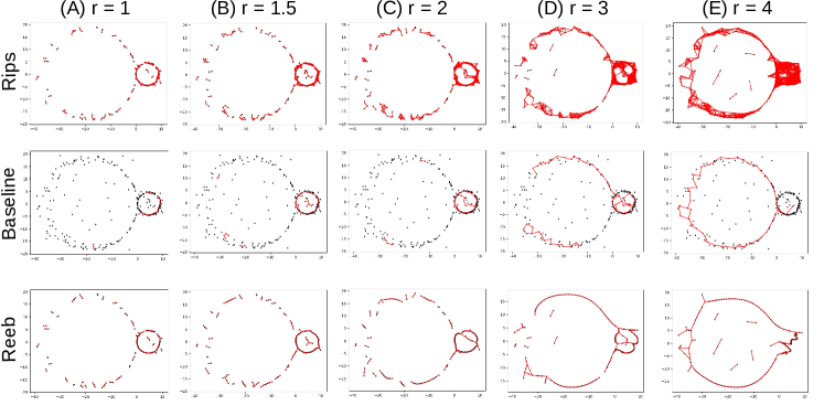
Figure 18: The ${\mathrm{rips}}^{r}(P)$ complex (first row), baseline outputs (second row), and ReebRecon outputs (third row). All baseline outputs were generated using persistence threshold zero, meaning that no simplification occurred. (A) $r=1$ - ${\mathrm{rips}}^{r}(P)$ complex fails to capture either circle, resulting in both methods failing to capture either circle. (B) $r=1.5$ - ${\mathrm{rips}}^{r}(P)$ complex now contains the smaller circle but not the larger circle. Both outputs successfully capture the smaller circle, but fail to capture the larger circle. (C) $r=2$ - ${\mathrm{rips}}^{r}(P)$ complex now connects the noise inside of the smaller circle to the smaller circle, while still not containing the larger circle. The outputs now capture the smaller circle and some noise inside of the circle, and still fail to capture the larger circle. (D) $r=3$ - ${\mathrm{rips}}^{r}(P)$ complex still does not contain the larger circle, and contains many edges cutting across the smaller circle. The ReebRecon output captures the smaller circle with more noise, while the baseline output has begun to lose the smaller circle. Both outputs fail to capture the larger circle. (E) $r=4$ - ${\mathrm{rips}}^{r}(P)$ complex now contains the larger circle, as well as a spurious loop, and the points forming the smaller circle now nearly form a clique. The outputs capture the larger circle, but contain a spurious loop, and the smaller circle is completely lost.

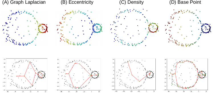
Figure 19: Two circle dataset: filter function values (first row) and corresponding Mapper outputs (second row) using (A) graph Laplacian filter ($k=15$), (B) eccentricity filter, (C) Gaussian density filter, (D) distance to base point filter.

Method	Radius	$\#$ Simplices	Time (seconds)
Our Method	$\infty$	19497	.06
Baseline	1	2182	.002
Reeb Graph	1	2182	.01
Baseline	2	8350	.013
Reeb Graph	2	8350	.02
Baseline	3	20005	.045
Reeb Graph	3	20005	.05
Baseline	4	41349	.13
Reeb Graph	4	41349	.25

Table 2: Two circle dataset: Comparison of running time of DM-PCD, baseline, and ReebRecon. Our algorithm has radius $\infty$ as we run on the full sparse DTM-Rips filtration.

Image patches dataset.  The main paper shows that our DM-PCD algorithm is able to successfully extract the "three-circle model" from a random 10,000 point subset of the image patches dataset from [8], while baseline, ReebRecon, and Mapper methods are unable to do so. We run baseline with ${\mathrm{rips}}^{.75}(P)$ as the input complex. We tried several $r$ values less than $.75$, as well as $r=.8$. For $r$ values less than $.75$, there were many spurious loops that could not be removed with persistence thresholding. For $r=.8$, the desired three-circles are not completely recovered even with no persistence thresholding. Results at various persistence thresholds are shown in Figure 20. Although the output does contain the three circles we wish to extract, it is also made up of several additional loops. Raising the persistence threshold to 5 removes some of the additional loops, but raising the persistence threshold to 10 removes part of the desired three circle model without removing the remaining additional loops. In fact, raising the persistence threshold to $\infty$, we see that some of these incorrect loops are a product of the input triangulation, and it is not possible to achieve a desired output from baseline with $r=.75$. While it may still be possible for a "good" $r$ value to exist, it is extremely expensive to compute persistence on triangulations with this many simplices.

Running time and simplicial complex size comparisons are shown in Table 3. For radius $r=.75$, we see that the number of simplices used in baseline is over 50,000,000 greater than the number of simplices in the filtration used by DM-PCD. Although DM-PCD takes longer to compute persistence even with a smaller filtration, the DM-PCD filtration has an implied $r=\infty$, and that any sizable increase to $r=.75$ for baseline will result in a significant increase in running time. We note that for all values of $r$, the number of simplices used in baseline would be the same number of simplices used by ReebRecon.

Additionally, the main paper shows that Mapper was unable to capture the true underlying structure of the image patches dataset. Further results for different filter functions are shown in Figure 21. Gaussian density and eccentricity filters fail, as seen in previous datasets. However, unlike the previous dataset, the graph Laplacian and distance to base point filters also fail to capture the underlying structure. This data is simply too noisy for Mapper to extract the underlying structure.

Finally, while our algorithm is deterministic, this dataset is generated from a random 10K point subset. In an attempt to quantify the error, we generated 10 different random subsets to apply our method to. On all 10 datasets, our method extracts the 3 circles correctly. To quantify error, we computed the distance between two output graphs $G_{i}$, $G_{j}$ by calculating the average distance between each node in one graph to its nearest node in the other graph, and normalizing this distance by the diameter of the full 50K point dataset. The result was $0.036$ average error.

Method	Radius	$\#$ Simplices	Time (seconds)
Our Method	$\infty$	209397755	16089.4
Baseline	.25	77261	.15
Baseline	.75	263787145	1485.42

Table 3: Image Patches dataset: Comparison of running time of DM-PCD and baseline. Our algorithm has radius $\infty$ as we run on the full sparse DTM-Rips filtration.

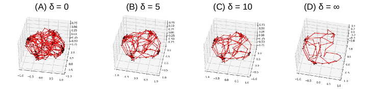
Figure 20: Image Patches: Outputs of baseline with ${\mathrm{rips}}^{r}(P)$ complex ($r=.75$) as the input triangulation at various persistence thresholds. (A) $\delta=0$ - With no thresholding of critical edges, the output captures the three circles that we expect to, as well as additional loops. (B) $\delta=5$ - Raising the persistence threshold allows for some of the additional loops to be removed while keeping the three circles we expect. (C) $\delta=10$ - Further raising the persistence threshold results in losing part of the horizontal circle while keeping extra loops. (D) $\delta=\inf$ - Removing all critical edges except those with infinity persistence removes more of the desired three circle output and keeps loops not part of the desired output.

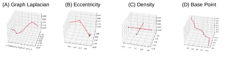
Figure 21: Image patches: Outputs of Mapper using different filter functions - (A) graph Laplacian filter ($k=15$), (B) eccentricity filter, (C) Gaussian density filter, (D), distance to base point filter. The dataset is too noisy and none of the filters result in Mapper outputting a graph representative of the true underlying structure.

Traffic flow dataset.  We also test on point clouds derived from traffic flow data [7]. We extract two datasets: the time-series of traffic flow at detector $\#$409529 from time-range 10/1/2017 to 10/14/2017 and from time-range 11/19/2017 to 12/2/2017 (which includes Thanksgiving). Each time-series is mapped to a point cloud dataset in ${\mathbb{R}}^{6}$ via time-delay embedding.

Given a time series $f:t->{\mathbb{R}}$ and a parameter $\tau$, the lift defined by $\phi(t)=(f(t),f(t+\tau),...,f(t+M\tau))$ is called a time delay embedding. For each traffic flow function, we create a PCD using a time delay embedding with $M=5$ and $\tau=50$. The two dimensional projections of these PCDs are shown in Figure 4 (B) of the main paper. The first function’s time delay embedding projection appears to be a single loop, while the second appears to have an inner loop and an outer loop.

The main paper shows the results of our DM-PCD algorithm with $k=30$ on both time series datasets. So far in our experiments, a default value of $k=15$ has been used. By the nature of time delay embeddings, which may create clumps of points close together, different values of $k$ can produce markedly different results. Shown in Figure 22 are results of DM-PCD on the two datasets with $k$ values of 15, 30, and 40. For the first dataset (10/1/2017 - 10/14/2017), a single loop is captured with all values of $k$. For the second dataset (11/19/2017 - 12/2/2017), changing the value of $k$ results in more drastic changes in the output. The persistence thresholds for the outputs are 8.25 ($k=15$), 12.5 ($k=30$), and 12.84 ($k=40$). In all cases, if the persistence threshold were raised enough to further threshold the output, a portion of the outer loop would be lost. We note that our output must be connected, so the desired result is two loops with a single connection. The output with $k=15$ contains many extra connections, while the output with $k=30$ contains a single extra connection. With $k=40$, the desired output is achieved.

Also shown in the main paper, baseline is able to successfully capture the single loop of the first time series dataset. Results for baseline on the second time series dataset are shown in Figure 23. The persistence thresholds for the outputs are 8 ($k=15$), 5 ($k=30$), and 3 ($k=40$). Just like the results for DM-PCD in Figure 22, if the persistence thresholds were raised enough to further threshold the output, a portion of the outer loop would be lost, making the output of DM-PCD superior.

Running time and simplicial complex size comparisons for 10/1/2017 - 10/14/2017 and 11/19/2017 - 12/2/2017 traffic flows are shown in Table 4 and 5 respectively. Note that the baseline results shown in the main paper use $r=90$ and $r=75$ respectively. For the first dataset, we see that the number of simplices used by the baseline with $r=90$ is more than five times greater than the number of simplices used in DM-PCD. This results in longer running time for baseline. For the second dataset, the number of simplices used by the baseline with $r=75$ is a little less than three times greater than the number of simplices used in DM-PCD. While the running time remained shorter for baseline in this particular instance, we note that an increase in the value of $r$ can add a significant amount of simplices and push the running time to be longer than the DM-PCD running time. We again note that for all values of $r$, the number of simplices used in baseline would be the same number of simplices used by ReebRecon.

Additionally, the main paper shows that Mapper was able to extract the structure behind traffic flow from 10/1/2017 to 10/14/2017, but was unable to do so for traffic flow from 11/19/2017 to 12/2/2017. Results of Mapper on both datasets using a variety of filter functions is shown in Figure 24. Again, using the graph Laplacian and distance to base point filters allowed Mapper to extract the single loop structure behind the first dataset. However, Mapper is unable to extract the two loop structure behind the second dataset with these filters, along with eccentricity and Gaussian density filters. In contrast, DM-PCD was able to get the true underlying structure behind both datasets.

Method	Radius	$\#$ Simplices	Time (seconds)
Our Method	$\infty$	6,879,338	98.6
Baseline	75	14,646,522	54.7
Baseline	90	35,543,784	123.903

Table 4: Traffic (10/1/2017 - 10/14/2017) dataset: comparison of running time of DM-PCD and baseline. Our algorithm has radius $\infty$ as we run on the full sparse DTM-Rips filtration.

Method	Radius	$\#$ Simplices	Time (seconds)
Our Method	$\infty$	5,720,309	106.1
Baseline	60	5,157,336	16.8
Baseline	75	15,659,797	57.7

Table 5: Traffic (11/19/2017 - 12/2/2017) dataset: comparison of running time of DM-PCD and baseline. Our algorithm has radius $\infty$ as we run on the full sparse DTM-Rips filtration.

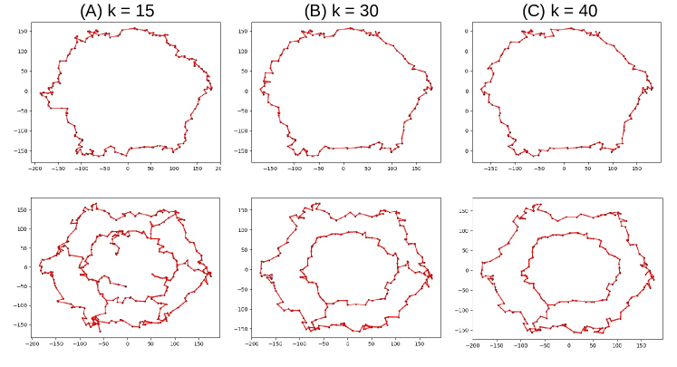
Figure 22: Traffic flow: Outputs of DM-PCD on both datasets (10/1/2017 - 10/14/2017 top row, 11/19/2017 - 12/2/2017 bottom row) with different values of $k$. (A) $k=15$ - Single loop captured in first dataset, two loops captured with extra connections in second dataset. (B) $k=30$ - Single loop captured in first dataset, two loops captured with an extra connection in second dataset. (C) $k=40$ - Single loop captured in first dataset, two loops captured with a single connection in second dataset.

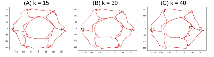
Figure 23: Traffic flow: Outputs of baseline method on the second traffic time series dataset (11/19/2017 - 12/2/2017) at different values of $k$ - (A) $k=15$, (B) $k=30$, (C) $k=40$. In all cases, any further simplification will lose the outer loop before removing any connections with the inner loop.

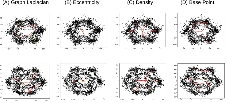
Figure 24: Traffic flow: Outputs of Mapper on both datasets using different filter functions - (A) graph Laplacian filter ($k=15$), (B) eccentricity filter, (C) Gaussian density filter, (D), distance to base point filter. The structure of traffic flow from 10/1/2017 to 10/14/2017 (first row) is captured by Mapper using the graph Laplacian filter function and the distance to base point filter function, while the structure of traffic flow from 11/19/2017 to 12/2/2017 (second row) is not captured by Mapper using any of the filter functions.

Coil-20.  Similarly to the two circle example, both the baseline and ReebRecon approaches are unable to capture all coils because the coils have varying scales in the original space. A concrete example is shown in Figure 25, where Objects 1 and 17 cannot be captured at the same scale. We also applied Mapper to Coil-17 using a base point filter. While Mapper can extract the structure of individual objects quite well, the method also struggles to capture all coils. Focusing on Objects 1 and 17 again, we see that by changing the epsilon parameter of the density clustering scheme we use inside of Mapper, we are able to capture the structure of either Object 1 or Object 17, but not both (results shown in Figure 26). While it may be possible that a different clustering scheme (or different covering and filter function combinations) could lead to a Mapper configuration that can capture both objects, finding parameters able to capture all coils would be difficult.

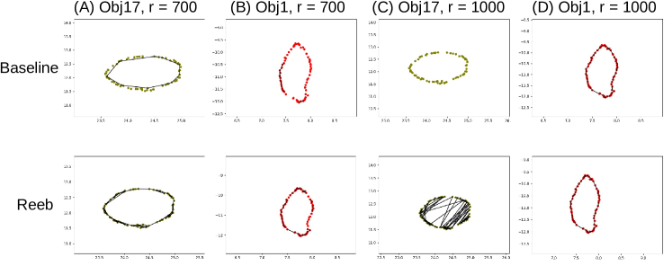
Figure 25: Coil: Objects 1 and 17 with baseline and ReebRecon outputs. (A) Object 17, $r=700$ - Object 17 is captured by both methods. (B) Object 1, $r=700$ - Object 1 is not captured by either method. (C) Object 17, $r=1000$ - Object 17 is not captured by either method. (D) Object 1, $r=1000$ - Object 1 is captured by both methods.

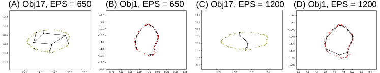
Figure 26: Coil: Objects 1 and 17 with Mapper outputs generated using a base point filter function. (A) Object 17, $EPS=650$ - structure of Object 17 is captured. (B) Object 1, $EPS=650$ - structure of Object 1 is not captured. (C) Object 17, $EPS=1200$ - structure of Object 17 is not captured. (D) Object 17, $EPS=1200$ - structure of Object 1 is captured.

References

- [1] M. Aanjaneya, F. Chazal, D. Chen, M. Glisse, L. Guibas, and D. Morozov. Metric graph reconstruction from noisy data. In Proc. 27th Sympos. Comput. Geom., pages 37–46, 2011.
- [2] S. Banerjee, L. Magee, D. Wang, X. Li, B. Huo, J. Jayakumar, K. Matho, M. Lin, K. Ram, M. Sivaprakasam, J. Huang, Y. Wang, and P. Mitra. Semantic segmentation of microscopic neuroanatomical data by combining topological priors with encoder-decoder deep networks. Nature Machine Intelligence, 2:585–594, 2020.
- [3] M. Belkin and P. Niyogi. Laplacian eigenmaps for dimensionality reduction and data representation. Neural Computation, 15(6):1373–1396, 2003.
- [4] Mikhail Belkin, Qichao Que, Yusu Wang, and X. Zhou. Toward understanding complex data: graph laplacians on manifolds with singularities and boundaries. In Conf. Learning Theory (COLT), pages 36.1–36.26, 2012. Journal of Machine Learning Research – Proceedings Track 23.
- [5] Mickaël Buchet, Frédéric Chazal, Steve Y. Oudot, and Donald R. Sheehy. Efficient and robust persistent homology for measures. In Proceedings of the Twenty-sixth Annual ACM-SIAM Symposium on Discrete Algorithms, SODA ’15, pages 168–180, Philadelphia, PA, USA, 2015. Society for Industrial and Applied Mathematics.
- [6] Chen Cai, Nikolaos Vlassis, Lucas Magee, Ran Ma, Zeyu Xiong, Bahador Bahmani, Teng-Fong Wong, Yusu Wang, and WaiChing Sun. Equivariant geometric learning for digital rock physics: estimating formation factor and effective permeability tensors from morse graph, 2021.
- [7] California Department of Transportation. Traffic flows at detector 409529, 2017.
- [8] Gunnar Carlsson, Tigran Ishkhanov, Vin Silva, and Afra Zomorodian. On the local behavior of spaces of natural images. International Journal of Computer Vision, 76:1–12, 01 2008.
- [9] F. Chazal, D. Cohen-Steiner, and Q. Mérigot. Geometric inference for probability measures. Foundations of Computational Mathematics, 11:733–751, 2011.
- [10] Frédéric Chazal, Ruqi Huang, and Jian Sun. Gromov—hausdorff approximation of filamentary structures using reeb-type graphs. Discrete Comput. Geom., 53(3):621–649, April 2015.
- [11] Frédéric Chazal, Vin de Silva, Marc Glisse, and Steve Oudot. The structure and stability of persistence modules. Springer, 2018.
- [12] David Cohen-Steiner, André Lieutier, and Julien Vuillamy. Lexicographic optimal chains and manifold triangulations, 2019. available at URL: https://hal.archives-ouvertes.fr/hal-02391190/document.
- [13] David Cohen-Steiner, André Lieutier, and Julien Vuillamy. Lexicographic optimal homologous chains and applications to point cloud triangulations. In 36th Sympos. Comput. Geom. (SoCG), 2020. to appear, see also url: https://hal.archives-ouvertes.fr/hal-02391240/document.
- [14] O. Delgado-Friedrichs, V. Robins, and A. Sheppard. Skeletonization and partitioning of digital images using discrete morse theory. IEEE Trans. Pattern Anal. Machine Intelligence, 37(3):654–666, March 2015.
- [15] T. K. Dey, J. Wang, and Y. Wang. Graph reconstruction by discrete morse theory. In Proc. Internat. Sympos. Comput. Geom., pages 31:1–31:15, 2018.
- [16] Tamal Dey, Jiayuan Wang, and Yusu Wang. Road network reconstruction from satellite images with machine learning supported by topological methods. In Proc. 27th ACM SIGSPATIAL Intl. Conf. Adv. Geographic Information Systems (GIS), pages 520–523, 2019.
- [17] Tamal K. Dey, Tao Hou, and Sayan Mandal. Computing minimal persistent cycles: Polynomial and hard cases. In Shuchi Chawla, editor, Proceedings of the 2020 ACM-SIAM Symposium on Discrete Algorithms, SODA 2020, Salt Lake City, UT, USA, January 5-8, 2020, pages 2587–2606. SIAM, 2020.
- [18] Tamal K. Dey, Jiayuan Wang, and Yusu Wang. Improved road network reconstruction using discrete morse theory. In Proc. 25th ACM SIGSPATIAL Intl. Conf. Adv. Geographic Information Systems (GIS), pages 58:1–58:4, 2017.
- [19] D.L. Donoho and C. Grimes. Hessian eigenmaps: Locally linear embedding techniques for high-dimensional data. Proceedings of the National Academy of Sciences, 100(10):5591–5596, 2003.
- [20] Herbert Edelsbrunner and John Harer. Computational Topology: An Introduction. Amer. Math. Soc., Providence, Rhode Island, 2010.
- [21] R. Forman. Combinatorial vector fields and dynamic systems. Mathematische Zeitschrift, 228(4):629–681, 1998.
- [22] Robin Forman. A user’s guide to discrete Morse theory. Séminare Lotharinen de Combinatore 48, 2002.
- [23] Xiaoyin Ge, Issam I. Safa, Mikhail Belkin, and Yusu Wang. Data skeletonization via reeb graphs. In J. Shawe-Taylor, R. S. Zemel, P. L. Bartlett, F. Pereira, and K. Q. Weinberger, editors, Advances in Neural Information Processing Systems 24, pages 837–845. Curran Associates, Inc., 2011.
- [24] A. Gyulassy, M. Duchaineau, V. Natarajan, V. Pascucci, E. Bringa, A. Higginbotham, and B. Hamann. Topologically clean distance fields. IEEE Trans. Visualization Computer Graphics, 13(6):1432–1439, Nov 2007.
- [25] T. J. Hastie. Principal curves and surfaces. PhD thesis, stanford university, 1984.
- [26] B. Kégl and A. Krzyżak. Piecewise linear skeletonization using principal curves. IEEE Trans. Pattern Anal. Machine Intell., 24:59–74, January 2002.
- [27] Fabrizio Lecci, Alessandro Rinaldo, and Larry Wasserman. Statistical analysis of metric graph reconstruction. J. Mach. Learn. Res., 15(1):3425–3446, January 2014.
- [28] A. Lee, K. Pedersen, and D. Mumford. The nonlinear statistics of high-contrast patches in natural images. International Journal of Computer Vision, 54:83–103, 2004.
- [29] Leland McInnes, John Healy, and James Melville. Umap: Uniform manifold approximation and projection for dimension reduction, 2020.
- [30] Nayar and H. Murase. Columbia object image library: Coil-100. Technical Report CUCS-006-96, Department of Computer Science, Columbia University, February 1996.
- [31] U. Ozertem and D. Erdogmus. Locally defined principal curves and surfaces. Journal of Machine Learning Research, 12:1249–1286, 2011.
- [32] Jose A. Perea and John Harer. Sliding windows and persistence: An application of topological methods to signal analysis. Found. Comput. Math. (FoCM), 15:799––838, 2015. https://doi.org/10.1007/s10208-014-9206-z.
- [33] V. Robins, P. J. Wood, and A. P. Sheppard. Theory and algorithms for constructing discrete morse complexes from grayscale digital images. IEEE Trans. Pattern Anal. Machine Intelligence, 33(8):1646–1658, Aug 2011.
- [34] S.T. Roweis and L.K. Saul. Nonlinear Dimensionality Reduction by Locally Linear Embedding. Science, 290(5500):2323, 2000.
- [35] Gurjeet Singh, Facundo Memoli, and Gunnar Carlsson. Topological Methods for the Analysis of High Dimensional Data Sets and 3D Object Recognition. In M. Botsch, R. Pajarola, B. Chen, and M. Zwicker, editors, Eurographics Symposium on Point-Based Graphics. The Eurographics Association, 2007.
- [36] Thierry Sousbie. The persistent cosmic web and its filamentary structure – i. theory and implementation. Monthly Notices of the Royal Astronomical Society, 414:350 – 383, 06 2011.
- [37] J.B. Tenenbaum, V. Silva, and J.C. Langford. A Global Geometric Framework for Nonlinear Dimensionality Reduction. Science, 290(5500):2319, 2000.
- [38] S. Wang, Y. Wang, and Y. Li. Efficient map reconstruction and augmentation via topological methods. In Proc. 23rd ACM SIGSPATIAL, page 25. ACM, 2015.
- [39] Pengxiang Wu, Chao Chen, Yusu Wang, Shaoting Zhang, Changhe Yuan, Zhen Qian, Dimitris N. Metaxas, and Leon Axel. Optimal topological cycles and their application in cardiac trabeculae restoration. In Information Processing in Medical Imaging - 25th International Conference, IPMI 2017, Boone, NC, USA, June 25-30, 2017, Proceedings, pages 80–92, 2017.