CONTaiNER: Few-Shot Named Entity Recognition via Contrastive Learning

Abstract

Named Entity Recognition (NER) in Few-Shot setting is imperative for entity tagging in low resource domains. Existing approaches only learn class-specific semantic features and intermediate representations from source domains. This affects generalizability to unseen target domains, resulting in suboptimal performances. To this end, we present CONTaiNER, a novel contrastive learning technique that optimizes the inter-token distribution distance for Few-Shot NER. Instead of optimizing class-specific attributes, CONTaiNER optimizes a generalized objective of differentiating between token categories based on their Gaussian-distributed embeddings. This effectively alleviates overfitting issues originating from training domains. Our experiments in several traditional test domains (OntoNotes, CoNLL’03, WNUT ’17, GUM) and a new large scale Few-Shot NER dataset (Few-NERD) demonstrate that, on average, CONTaiNER outperforms previous methods by 3%-13% absolute F1 points while showing consistent performance trends, even in challenging scenarios where previous approaches could not achieve appreciable performance. The source code of CONTaiNER will be available at: https://github.com/psunlpgroup/CONTaiNER.

1 Introduction

Named Entity Recognition (NER) is a fundamental NLU task that recognizes mention spans in unstructured text and categorizes them into a pre-defined set of entity classes. In spite of its challenging nature, recent deep-learning based approaches Huang et al. (2015); Ma and Hovy (2016); Lample et al. (2016); Peters et al. (2018); Devlin et al. (2018) have achieved impressive performance. As these supervised NER models require large-scale human-annotated datasets, few-shot techniques that can effectively perform NER in resource constraint settings have recently garnered a lot of attention.

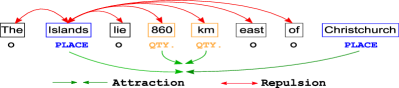
Figure 1: Contrastive learning dynamics of a token (Islands) with all other tokens in an example sentence from GUM Zeldes (2017). CONTaiNER decreases the embedding distance between tokens of the same category (PLACE) while increasing the distance between different categories ( QTY. and O).

Few-shot learning involves learning unseen classes from very few labeled examples Fei-Fei et al. (2006); Lake et al. (2011); Bao et al. (2020). To avoid overfitting with the limited available data, meta-learning has been introduced to focus on how to learn Vinyals et al. (2016); Bao et al. (2020). Snell et al. (2017) proposed Prototypical Networks to learn a metric space where the examples of a specific unknown class cluster around a single prototype. Although it was primarily deployed in computer vision, Fritzler et al. (2019) and Hou et al. (2020) also used Prototypical Networks for few-shot NER. Yang and Katiyar (2020), on the other hand, proposed a supervised NER model that learns class-specific features and extends the intermediate representations to unseen domains. Additionally, they employed a Viterbi decoding variant of their model as "StructShot".

Few-shot NER poses some unique challenges that make it significantly more difficult than other few-shot learning tasks. First, as a sequence labeling task, NER requires label assignment according to the concordant context as well as the dependencies within the labels Lample et al. (2016); Yang and Katiyar (2020). Second, in NER, tokens that do not refer to any defined set of entities are labeled as Outside (O). Consequently, a token that is labeled as O in training entity set may correspond to a valid target entity in test set. For prototypical networks, this challenges the notion of entity examples being clustered around a single prototype. As for Nearest Neighbor based methods such as Yang and Katiyar (2020), they are initially “pretrained" with the objective of source class-specific supervision. As a result, the trained weights will be closely tied to the source classes and the network will project training set O-tokens so that they get clustered in embedding space. This will force the embeddings to drop a lot of useful features pertaining to its true target entity in the test set. Third, in few-shot setting, there are not enough samples from which we can select a validation set. This reduces the capability of hyperparameter tuning, which particularly affects template based methods where prompt selection is crucial for good performance Cui et al. (2021). In fact, the absence of held-out validation set puts a lot of earlier few-shot works into question whether their strategy is truly "Few-Shot" Perez et al. (2021).

To deal with these challenges, we present a novel approach , CONTaiNER that harnesses the power of contrastive learning to solve Few-Shot NER. CONTaiNER tries to decrease the distance of token embeddings of similar entities while increasing it for dissimilar ones (Figure 1). This enables CONTaiNER to better capture the label dependencies. Also, since CONTaiNER is trained with a generalized objective, it can effectively avoid the pitfalls of O-tokens that the prior methods struggle with. Lastly, CONTaiNER does not require any dataset specific prompt or hyperparameter tuning. Standard settings used in prior works Yang and Katiyar (2020) works well across different domains in different evaluation settings.

Unlike traditional contrastive learners Chen et al. (2020); Khosla et al. (2020) that optimize similarity objective between point embeddings, CONTaiNER optimizes distributional divergence effectively modeling Gaussian Embeddings. While point embedding simply optimizes sample distances, Gaussian Embedding faces an additional constraint of maintaining class distribution through the variance estimation. Thus Gaussian Embedding explicitly models entity class distributions which not only promotes generalized feature representation but also helps in few-sample target domain adaptation. Previous works in Gaussian Embedding has also shown that mapping to a density captures representation uncertainties Vilnis and McCallum (2014) and expresses natural asymmetries Qian et al. (2021) while showing better generalization requiring less data to achieve optimal performance Bojchevski and Günnemann (2017). Inspired by these unique qualities of Gaussian Embedding, in this work we leverage Gaussian Embedding in contrastive learning for Few-Shot NER.

A nearest neighbor classification scheme during evaluation reveals that on average, CONTaiNER significantly outperforms previous SOTA approaches in a wide range of tests by up to 13% absolute F1-points. In particular, we extensively test our model in both in-domain and out-of-domain experiments as proposed in Yang and Katiyar (2020) in various datasets (CoNLL ’03, OntoNotes 5.0, WNUT ’17, I2B2). We also test our model in a large dataset recently proposed for Few-Shot NER - Few-NERD Ding et al. (2021) where CONTaiNER outperforms all other SOTA approaches setting a new benchmark result in the leaderboard.

In summary, our contributions are as follows: (1) We propose a novel Few-Shot NER approach CONTaiNER that leverages contrastive learning to infer distributional distance of their Gaussian Embeddings. To the best of our knowledge we are the first to leverage Gaussian Embedding in contrastive learning for Named Entity Recognition. (2) We demonstrate that CONTaiNER representations are better suited for adaptation to unseen novel classes, even with a low number of support samples. (3) We extensively test CONTaiNER in a wide range of experiments using several datasets and evaluation schemes. In almost every case, our model largely outperforms present SOTAs establishing new benchmark results.

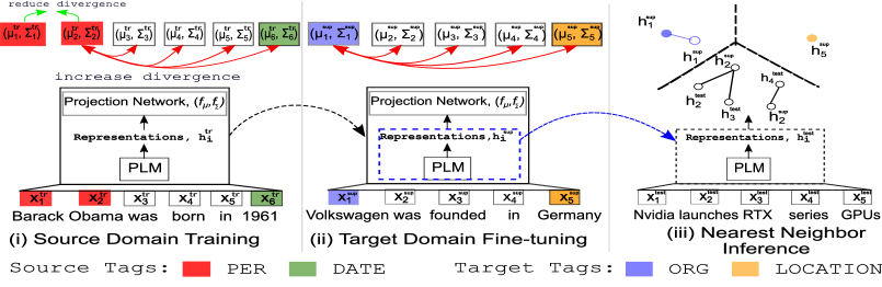
Figure 2: Illustration of our proposed CONTaiNER framework based on Contrastive Learning over Gaussian Embedddings: (i) Training in source domains using training NER labels PER and DATE, (ii) Fine-tuning to target domains using target NER labels ORG and LOCATION, (iii) Assigning labels to test samples via Nearest Neighbor support set labels.

2 Task Formulation

Given a sequence of $n$ tokens $\{x_{1},x_{2},\ldots x_{n}\}$, NER aims to assign each token $x_{i}$ to its corresponding tag label $y_{i}$.

Few-shot Setting

For Few-shot NER, a model is trained in a source domain with a tag-set $\{C_{(i)}^{s}\}$ and tested in a data-scarce target domain with a tag-set $\{C_{(j)}^{d}\}$ where $i,j$ are index of different tags. Since $\{C_{(i)}^{s}\}\cap\{C_{(j)}^{d}\}=\emptyset$, it is very challenging for models to generalize to unseen test tags. In an N-way K-shot setting, there are $N$ tags in the target domain $|\{C_{(j)}^{d}\}|=N$, and each tag is associated with a support set with K examples.

Tagging Scheme

For fair comparison of CONTaiNER against previous SOTA models, we follow an IO tagging scheme where I-type represents that all of the tokens are inside an entity, and O-type denotes all the other tokens Yang and Katiyar (2020); Ding et al. (2021).

Evaluation Scheme

To compare with SOTA models in Few-NERD leaderboard Ding et al. (2021), we adpot episode evaluation as done by the authors. Here, a model is assessed by calculating the micro-F1 score over multiple number of test episodes. Each episode consists of a K-shot support set and a K-shot unlabeled query (test) set to make predictions. While Few-NERD is explicitly designed for episode evaluation, traditional NER datasets (e.g., OntoNotes, CoNLL’03, WNUT ’17, GUM) have their distinctive tag-set distributions. Thus, sampling test episodes from the actual test data perturbs the true distribution that may not represent the actual performance. Consequently, Yang and Katiyar (2020) proposed to sample multiple support sets from the original development set and use them for prediction in the original test set. We also use this evaluation strategy for these traditional NER datasets.

3 Method

CONTaiNER utilizes contrastive learning to optimize distributional divergence between different token entity representations. Instead of focusing on label specific attributes, this contradistinction explicitly trains the model to distinguish between different categories of tokens. Furthermore, modeling Gaussian Embedding instead of traditional point representation effectively lets CONTaiNER model the entity class distribution, which incites generalized representation of tokens. Finally, it lets us carefully finetune our model even with a small number of samples without overfitting which is imperative for domain adaptation.

As demonstrated in Figure 2, we first train our model in source domains. Next, we finetune model representations using few-sample support sets to adapt it to target domains. The training and finetuning of CONTaiNER is illustrated in Algorithm 1. Finally, we use an instance level nearest neighbor classifier for inference in test sets.

3.1 Model

Figure 2 shows the key components of our model. To generate contextualized representation of sentence tokens, CONTaiNER incorporates a pretrained language model encoder PLM. For proper comparison against existing approaches, we use BERT Devlin et al. (2018) as our PLM encoder. Thus given a sequence of $n$ tokens $[x_{1},x_{2},\ldots,x_{n}]$, we take the final hidden layer output of the PLM as the intermediate representations $\bm{h}_{i}\in\mathbb{R}^{l^{\prime}}$.

$$[\bm{h}_{1},\bm{h}_{2},\ldots,\bm{h}_{n}]=\texttt{PLM}([x_{1},x_{2},\ldots,x_{n}])$$ (1)

These intermediate representations are then channeled through simple projection layer for generating the embedding. Unlike SimCLR Chen et al. (2020) that uses projected point embedding for contrastive learning, we assume that token embeddings follow Gaussian distributions. Specifically, we employ projection network $f_{\mu}$ and $f_{\Sigma}$ for producing Gaussian distribution parameters:

$$\bm{\mu}_{i}=f_{\mu}(\bm{h}_{i}),~{}~{}\bm{\Sigma}_{i}=\operatorname*{ELU}\left(f_{\Sigma}(\bm{h}_{i})\right)+(1+\epsilon)$$ (2)

where $\bm{\mu}_{i}\in\mathbb{R}^{l},\bm{\Sigma}_{i}\in\mathbb{R}^{l\times l}$ represents mean and diagonal covariance (with nonzero elements only along the diagonal of the matrix) of the Gaussian Embedding respectively; $f_{\mu}$ and $f_{\Sigma}$ are implemented as ReLU followed by single layer networks; $\operatorname*{ELU}$ for exponential linear unit; and $\epsilon\approx e^{-14}$ for numerical stability.

3.2 Training in Source Domain

For calculating the contrastive loss, we consider the KL-divergence between all valid token pairs in the sampled batch. Two tokens $x_{p}$ and $x_{q}$ are considered as positive examples if they have the same label $y_{p}=y_{q}$. Given their Gaussian Embeddings $\mathcal{N}(\bm{\mu}_{p},\bm{\Sigma}_{p})$ and $\mathcal{N}(\bm{\mu}_{q},\bm{\Sigma}_{q})$, we can calculate their KL-divergence as following:

$$\begin{split}D_{\text{KL}}&[\mathcal{N}_{q}||\mathcal{N}_{p}]=D_{\text{KL}}[\mathcal{N}(\bm{\mu}_{q},\bm{\Sigma}_{q})||\mathcal{N}(\bm{\mu}_{p},\bm{\Sigma}_{p})]\\ &=\frac{1}{2}\biggl{(}\operatorname{Tr}(\bm{\Sigma}_{p}^{-1}\bm{\Sigma}_{q})\\ &\quad\quad+(\bm{\mu}_{p}-\bm{\mu}_{q})^{T}\bm{\Sigma}_{p}^{-1}(\bm{\mu}_{p}-\bm{\mu}_{q})\\ &\quad\quad-l+\log\frac{|\bm{\Sigma}_{p}|}{|\bm{\Sigma}_{q}|}\biggr{)}\end{split}$$ (3)

Both directions of the KL-divergence are calculated since it is not symmetric.

$$d(p,q)=\frac{1}{2}\left(D_{\text{KL}}[\mathcal{N}_{q}||\mathcal{N}_{p}]+D_{\text{KL}}[\mathcal{N}_{p}||\mathcal{N}_{q}]\right)$$ (4)

We first train our model in resource rich source domain having training data $\mathcal{X}_{\text{tr}}$. At each training step, we randomly sample a batch of sequences (without replacement) $\mathcal{X}\in\mathcal{X}_{\text{tr}}$ from the training set having batch size of $b$. For each $(x_{i},y_{i})\in\mathcal{X}$, we obtain its Gaussian Embedding $\mathcal{N}(\mu_{i},\Sigma_{i})$ by channeling the corresponding token sequence through the model (Algorithm 1: Line 3-6). We find in-batch positive samples $\mathcal{X}_{p}$ for sample $p$ and subsequently calculate the Gaussian embedding loss of $x_{p}$ with respect to that of all other valid tokens in the batch:

$$\begin{split}\mathcal{X}_{p}=\{(x_{q},y_{q})\in\mathcal{X}\mid y_{p}=y_{q},p\neq q\}\\ \end{split}$$ (5)

$$\ell(p)=-\log\frac{\sum\limits_{\begin{subarray}{c}(x_{q},y_{q})\in\mathcal{X}_{p}\end{subarray}}\exp(-d(p,q))/|\mathcal{X}_{p}|}{\sum\limits_{\begin{subarray}{c}(x_{q},y_{q})\in\mathcal{X},p\neq q\end{subarray}}\exp(-d(p,q))}$$ (6)

In this way we can calculate the distributional divergence of all the token pairs in the batch (Algorithm 1: Line 7-10 ). We do not scale the contrastive loss by any normalization factor as proposed by Chen et al. (2020) since we did not find it to be beneficial for optimization.

3.3 Finetuning to Target Domain using Support Set

After training in source domains, we finetune our model using a small number of target domain support samples following a similar procedure as in the training stage. As we have only a few samples for finetuning, we take them in a single batch. When multiple few-shot samples (e.g., 5-shot) are available for the target classes, the model can effectively adapt to the new domain by optimizing KL-divergence of Gaussian Embeddings as in Eq. 4. In contrast, for 1-shot case, it turns out challenging for models to adapt to the target class distribution. If the model has no prior knowledge about target classes (either from direct training or indirectly from source domain training where the target class entities are marked as O-type), a single example might not be sufficient to deduce the variance of the target class distribution. Thus, for 1-shot scenario, we optimize $d^{\prime}(p,q)=||\bm{\mu}_{p}-\bm{\mu}_{q}||_{2}^{2}$, the squared euclidean distance between mean of the embedding distributions. When the model has direct/indirect prior knowledge about the target classes involved, we still optimize the KL-divergence of the distributions similar to the 5-shot scenario.

We demonstrate in Table 7 that optimizing with squared euclidean distance gives us slightly better performance in 1-shot scenario. Nevertheless, in all cases with 5-shot support set, optimizing the KL-divergence between the Gaussian Embeddings gives us the best result.

Early Stopping

Finetuning with a small support set runs the risk of overfitting and without access to a held out validation set due to data scarcity in the target domain, we cannot keep tabs on the saturation point where we need to stop finetuning. To alleviate this, we rely on the calculated contrastive loss and use it as our early stopping criteria with a patience of 1. (Algorithm 1: Line 16-17, 24 )

Algorithm 1 Training and Finetuning of CONTaiNER

0:  Training data $\mathcal{X}_{tr}$, Support Data $\mathcal{X}_{sup}$, Train loss function $d_{tr}$, Finetune loss function $d_{ft}$ , $f_{\mu},f_{\Sigma}$, PLM

1:  // training in source domain

2:  for sampled (w/o replacement) minibatch $\mathcal{X}\in\mathcal{X}_{tr}$  do

3:     for all $i\equiv(x_{i},y_{i})\in\mathcal{X}$ do

4:        $\bm{\mu}_{i}=f_{\mu}(\texttt{PLM}(x_{i}))$ //[Eq. 1]

5:        $\bm{\Sigma}_{i}=ELU(f_{\Sigma}(\texttt{PLM}(x_{i})))+(1+\epsilon)$ //[Eq. 2]

6:     end for

7:     for all $i\equiv(x_{i},y_{i})\in\mathcal{X}$ do

8:        Calculate $\ell(i)$ as in Eq. 5 and 6

9:     end for

10:     $\mathcal{L}_{tr}=\frac{1}{|\mathcal{X}|}\sum\limits_{i\in\mathcal{X}}\ell(i)$

11:     update $f_{\mu},f_{\Sigma},$ PLM by backpropagation to reduce $\mathcal{L}_{tr}$

12:  end for

13:  // finetuning to target domain

14:  $\mathcal{L}_{prev}=\infty$

15:  $\mathcal{L}_{ft}=\mathcal{L}_{prev}-1$ //Stable Initialization

16:  while $\mathcal{L}_{ft}<\mathcal{L}_{prev}$ do

17:     $\mathcal{L}_{prev}=\mathcal{L}_{ft}$

18:     for all $i\equiv(x_{i},y_{i})\in\mathcal{X}_{sup}$ do

19:        Calculate $\bm{\mu}_{i}$ and $\bm{\Sigma}_{i}$ using Eq. 1, 2 //Line 4,5

20:     end for

21:     for all $i\equiv(x_{i},y_{i})\in\mathcal{X}_{sup}$ do

22:        Calculate $\ell(i)$ as in Eq. 5 and 6

23:     end for

24:     $\mathcal{L}_{ft}=\frac{1}{|\mathcal{X}_{sup}|}\sum\limits_{i\in\mathcal{X}_{sup}}\ell(i)$

25:     update $f_{\mu},f_{\Sigma},$ PLM by backpropagation to reduce $\mathcal{L}_{ft}$

26:  end while

27:  return  PLM and discard $f_{\mu}$, $f_{\Sigma}$

3.4 Instance Level Nearest Neighbor Inference

After training and finetuning the network with train and support data respectively, we extract the pretrained language model encoder PLM for inference. Similar to SimCLR Chen et al. (2020), we found that representations before the projection layers actually contain more information than the final output representation which contributes to better performance, so $f_{\mu}$ and $f_{\Sigma}$ projection heads are not used for inference. We thus calculate the representations of the test data from PLM and find nearest neighbor support set representation for inference Wang et al. (2019); Yang and Katiyar (2020).

The PLM representations $\bm{h}_{j}^{\text{sup}}$ of each of the support token $(x_{j}^{\text{sup}},y_{j}^{\text{sup}})\in\mathcal{X}_{\text{sup}}$ can be calculated as in Eq. 1. Similarly for test data $\mathcal{X}_{\text{test}}$, we get the PLM representations $\bm{h}_{i}^{\text{test}}$ where $x_{i}^{\text{test}}\in\mathcal{X}_{\text{test}}$. Here we assign $x_{i}^{\text{test}}$ the same label as the support token that is nearest in the PLM representation space:

$$y_{i}^{\text{test}}=\operatorname*{arg\,min}\limits_{y_{k}^{\text{sup}}~{}\text{where}~{}(x_{k}^{\text{sup}},y_{k}^{\text{sup}})\in\mathcal{X}_{\text{sup}}}||\bm{h}_{i}^{\text{test}}-\bm{h}_{k}^{\text{sup}}||_{2}^{2}$$ (7)

Dataset	Domain	# Class	# Sent
OntoNotes	General	18	76K
I2B2’14	Medical	23	140K
CoNLL’03	News	4	20K
WNUT’17	Social	6	5K
GUM	Mixed	11	3.5K
Few-NERD	Wikipedia	66	188K

Table 1: Summary Statistics of Datasets

Viterbi Decoding

Most previous works Hou et al. (2020); Yang and Katiyar (2020); Ding et al. (2021) noticed a performance improvement by using CRFs Lafferty et al. (2001) which removes false predictions to improve performance. Thus we also employ Viterbi decoding in the inference stage with an abstract transition distribution as in StructShot Yang and Katiyar (2020). For the transition probabilities, the transition between three abstract tags O, I, and I-other is estimated by counting their occurrences in the training set. Then for the target domain tag-set, these transition probabilities are evenly distributed into corresponding target distributions. The emission probabilities are calculated from Nearest Neighbor Inference stage. Comparing domain transfer results (Table 3) against other tasks (Table 2,4,5) we find that, interestingly, if there is no significant domain shift involved in the test data, contrastive learning allows CONTaiNER to automatically extract label dependencies, obviating the requirement of extra Viterbi decoding stage.

4 Experiment Setups

Datasets

For evaluation, we use datasets across different domains: General (OntoNotes 5.0 Weischedel et al. (2013)), Medical (I2B2 Stubbs and Uzuner (2015)), News (CoNLL’03 Sang and De Meulder (2003)), Social (WNUT’17 Derczynski et al. (2017)). We also test on GUM Zeldes (2017) that represents wide variety of texts: interviews, news articles, instrumental texts, and travel guides. The miscellany of domains makes it a challenging dataset to work on. Ding et al. (2021) argue that the distribution of these datasets may not be suitable for proper representation of Few-Shot capability. Thus, they proposed a new large scale dataset Few-NERD that contains 66 fine-grained entities across 8 coarse grained entities, significantly richer than previous datasets. A summary of these datasets is given in Table 1.

Baselines

Model	1-shot				5-shot
	Group A	Group B	Group C	Avg.	Group A	Group B	Group C	Avg.
Proto	19.3 $\pm$ 3.9	22.7 $\pm$ 8.9	18.9 $\pm$ 7.9	20.3	30.5 $\pm$ 3.5	38.7 $\pm$ 5.6	41.1 $\pm$ 3.3	36.7
NNShot	28.5 $\pm$ 9.2	27.3 $\pm$ 12.3	21.4 $\pm$ 9.7	25.7	44.0 $\pm$ 2.1	51.6 $\pm$ 5.9	47.6 $\pm$ 2.8	47.7
StructShot	30.5 $\pm$ 12.3	28.8 $\pm$ 11.2	20.8 $\pm$ 9.9	26.7	47.5 $\pm$ 4.0	53.0 $\pm$ 7.9	48.7 $\pm$ 2.7	49.8
CONTaiNER	32.2 $\pm$ 5.3	30.9 $\pm$ 11.6	32.9 $\pm$ 12.7	32.0	51.2 $\pm$ 5.9	55.9 $\pm$ 6.2	61.5 $\pm$ 2.7	56.2
+ Viterbi	32.4 $\pm$ 5.1	30.9 $\pm$ 11.6	33.0 $\pm$ 12.8	32.1	51.2 $\pm$ 6.0	56.0 $\pm$ 6.2	61.5 $\pm$ 2.7	56.2

Table 2: F1 scores in Tag Set Extension on OntoNotes. Group A, B, C are three disjoint sets of entity types. Results vary slightly compared to Yang and Katiyar (2020) since they used different support set samples (publicly unavailable) than ours.

Model	1-shot					5-shot
	I2B2	CoNLL	WNUT	GUM	Avg.	I2B2	CoNLL	WNUT	GUM	Avg.
Proto	13.4 $\pm$ 3.0	49.9 $\pm$ 8.6	17.4 $\pm$ 4.9	17.8 $\pm$ 3.5	24.6	17.9 $\pm$ 1.8	61.3 $\pm$ 9.1	22.8 $\pm$ 4.5	19.5 $\pm$ 3.4	30.4
NNShot	15.3 $\pm$ 1.6	61.2 $\pm$ 10.4	22.7 $\pm$ 7.4	10.5 $\pm$ 2.9	27.4	22.0 $\pm$ 1.5	74.1 $\pm$ 2.3	27.3 $\pm$ 5.4	15.9 $\pm$ 1.8	34.8
StructShot	21.4 $\pm$ 3.8	62.4 $\pm$ 10.5	24.2 $\pm$ 8.0	7.8 $\pm$ 2.1	29.0	30.3 $\pm$ 2.1	74.8 $\pm$ 2.4	30.4 $\pm$ 6.5	13.3 $\pm$ 1.3	37.2
CONTaiNER	16.4 $\pm$ 1.7	57.8 $\pm$ 10.7	24.2 $\pm$ 2.9	17.9 $\pm$ 1.8	29.1	24.1 $\pm$ 1.9	72.8 $\pm$ 2.0	27.7 $\pm$ 2.2	24.4 $\pm$ 2.2	37.3
+ Viterbi	21.5 $\pm$ 1.7	61.2 $\pm$ 10.7	27.5 $\pm$ 1.9	18.5 $\pm$ 4.9	32.2	36.7 $\pm$ 2.1	75.8 $\pm$ 2.7	32.5 $\pm$ 3.8	25.2 $\pm$ 2.7	42.6

Table 3: F1 scores in Domain Extension with OntoNotes as the source domain. Results vary slightly compared to Yang and Katiyar (2020) since they used different support set samples (publicly unavailable) than ours.

We compare the performance of CONTaiNER with state-of-the-art Few-Shot NER models on different datasets across several settings. We first measure the model performance in traditional NER datasets in tag-set extension and domain transfer tasks as proposed in Yang and Katiyar (2020). We then evaluate our model in Few-NERD Ding et al. (2021) dataset that is explicitly designed for Few-Shot NER, and compare it against the Few-NERD leaderboard baselines. Similar to Ding et al. (2021), we take Prototypical Network based ProtoBERT Snell et al. (2017); Fritzler et al. (2019); Hou et al. (2020), nearest neighbor based metric method NNShot that leverages the locality of in-class samples in embedding space, and additional Viterbi decoding based Structshot Yang and Katiyar (2020) as the main SOTA baselines.

4.1 Tag-set Extension Setting

A common use-case of Few-Shot NER is that new entity types may appear in the same existing text domain. Thus (Yang and Katiyar, 2020) proposed to experiment tag-set extension capability using OntoNotes Weischedel et al. (2013) dataset. The eighteen existing entity classes are split in three groups: A, B, and C, each having six classes. Models are tested in each of these groups having few sample support set while being trained in the remaining two groups. During training, all test group entities are replaced with O-tag. Since the source and destination domains are the same, the training phase will induce some indirect information about unseen target entities. So, during finetuning of CONTaiNER, we optimize the KL-divergence between ouptut embeddings as in Eq. 4.

We use the same entity class splits as used by Yang and Katiyar (2020) and used bert-base-cased as the backbone encoder for all models. Since they could not share the sampled support set for licensing reasons, we sampled five sets of support samples for each group and averaged the results, as done by the authors. We show these results in Table 2. We see that in different entity groups, CONTaiNER outperforms present SOTAs by upto 12.75 absolute F1 points, a substantial improvement in performance.

4.2 Domain Transfer Setting

In this experiment a model trained on a source domain is deployed to a previously unseen novel text domain. Here we take OntoNotes (General) as our source text domain, and evaluate the Few-Shot performance in I2B2 (Medical), CoNLL (News), WNUT (Social) domains as in Yang and Katiyar (2020). We also evaluate the performance in GUM Zeldes (2017) dataset due to its particularly challenging nature. We show these results in Table 3. While all the other domains have almost no intersection with OntoNotes, target entities in CoNLL are fully contained within OntoNotes entities, that makes it comparable to supervised learning.

4.3 Few-NERD Setting

For few-shot setting, Ding et al. (2021) proposed two different settings: Few-NERD (INTRA) and Few-NERD (INTER). In Few-NERD (INTRA) train, dev, and test sets are divided according to coarse-grained types. As a result, fine-grained entity types belonging to People, Art, Product, MISC coarse grained types are put in the train set, Event, Building coarse grained types in dev set, and ORG, LOC in test set. So, there is no overlap between train, dev, test set classes in terms of coarse grained types. On the other hand, in Few-NERD (INTER) coarse grained types are shared, although all the fine grained types are mutually disjoint. Because of the restrictions of sharing coarse-grained types, Few-NERD (INTRA) is more challenging.

Model	5-way		10-way		Avg.
	1$\sim$2 shot	5$\sim$10 shot	1$\sim$2 shot	5$\sim$10 shot
StructShot	35.92	38.83	25.38	26.39	31.63
ProtoBERT	23.45	41.93	19.76	34.61	29.94
NNShot	31.01	35.74	21.88	27.67	29.08
CONTaiNER	40.43	53.70	33.84	47.49	43.87
+ Viterbi	40.40	53.71	33.82	47.51	43.86

Table 4: F1 scores in FEW-NERD (INTRA).

Model	5-way		10-way		Avg.
	1$\sim$2 shot	5$\sim$10 shot	1$\sim$2 shot	5$\sim$10 shot
StructShot	57.33	57.16	49.46	49.39	53.34
ProtoBERT	44.44	58.80	39.09	53.97	49.08
NNShot	54.29	50.56	46.98	50.00	50.46
CONTaiNER	55.95	61.83	48.35	57.12	55.81
+ Viterbi	56.1	61.90	48.36	57.13	55.87

Table 5: F1 scores in FEW-NERD (INTER).

Since, few-shot performance of any model relies on the sampled support set, the authors also released train, dev, test split for both Few-NERD (INTRA) and Few-NERD (INTER). We evaluate our model performance using these provided dataset splits and compare the performance in Few-NERD leaderboard. All models use bert-base-uncased as the backbone encoder. As shown in Table 4 and Table 5, CONTaiNER establishes new benchmark results in the leaderboard in both of these tests.

5 Results and Analysis

We prudently analyze different components of our model and justify the design choices made in the scheming of CONTaiNER. We also examine the results discussed in Section 4 that gives some intuitions about few-shot NER in general.

5.1 Overall Results

Table 2-5 demonstrates that overall, in every scenario CONTaiNER convincingly outperforms all other baseline approaches. This improvement is particularly noticeable in challenging scenarios, where all other baseline approaches perform poorly. For example, FEW-NERD (intra) (Table 4) is a challenging scenario where the coarse grained entity types corresponding to train and test sets do not overlap. As a result, other baseline approaches face a substantial performance hit, whereas CONTaiNER still performs well. In tag-set extension (Table 2), we see a similar performance trend - CONTaiNER performs consistently well across the board. Likewise, in domain transfer to a very challenging unseen text domain like GUM Zeldes (2017), baseline models performs miserably; yet CONTaiNER manages to perform consistently outperforming SOTA models by a significant margin. Analyzing these results more closely, we notice that while CONTaiNER surpasses other baselines in almost every tests, more prominently in 5-shot cases. Evidently, CONTaiNER is able to make better use of multiple few-shot samples thanks to distribution modeling via contrastive Gaussian Embedding optimization. In this context, note that StructShot actually got marginally higher F1-score in 1-shot CoNLL domain adaptation and 1$\sim$2 shot FEW-NERD (INTER) cases. In CoNLL, the target classes are subsets of training classes, so supervised learning based feature extractors are expected to get an advantage in prediction. On the other hand, Ding et al. (2021) carefully tuned the hyperparameters for baselines like StructShot for best performance. We could also improve performance in a similar manner, however for uniformity of model across different few-shot settings, we use the same model architecture in every test. Nevertheless, CONTaiNER shows comparable performance even in these cases while significantly outperforming in every other test.

5.2 Training Objective

Traditional contrastive learners usually optimize cosine similarity of point embeddings Chen et al. (2020). While this has proven to work well in image data, in more challenging NLU tasks like Few-Shot NER, it gives subpar performance. We compare the performance of point embeddings with euclidean distance and cosine similarity to that of CONTaiNER using Gaussian Embedding and KL-divergence in OntoNotes tag-set extension. We report these performance in Table 8 in Appendix. Basically, Gaussian Embedding leads to learning generalized representation during training, which is more suitable for finetuning to few sample target domain. In Appendix C, we examine this aspect by comparing the t-SNE representations from point embedding and Gaussian Embedding.

5.3 Effect of Model Fine-tuning

Being a contrastive learner, CONTaiNER can take advantage of extremely small support set to refine its representations through fine-tuning. To closely examine the effects of fine-tuning, we conduct a case study with OntoNotes tag-extension task using PERSON, DATE, MONEY, LOC, FAC, PRODUCT target entities.

	W/O Finetuning	W/ Finetuning
1-shot	31.76	32.90
5-shot	56.99	61.48

Table 6: Comparison of F1-Scores with and without support set finetuning of CONTaiNER

As shown in Table 6, we see that finetuning indeed improves few-shot performance. Besides, the effect of finetuning is even more marked in 5-shot prediction indicating that CONTaiNER finetuning process can make the best use of few-samples available in target domain.

5.4 Modeling Label Dependencies

Analyzing the results, we observe that domain transfer (Table 3) sees some good gains in performance from using Viterbi decoding. In contrast, tag-set extension (Table 2) and FEW-NERD (Table 4,5) gets almost no improvement from using Viterbi decoding. This indicates an interesting property of CONTaiNER. During domain transfer the text domains have no overlap in train and test set. So, an extra Viterbi decoding actually provides additional information regarding the label dependencies, giving us some nice improvement. Otherwise, the train and target domain have substantial overlap in both tagset extension and FEW-NERD. Thus the model can indirectly learn the label dependencies through in-batch contrastive learning. Consequently, unless there is a marked shift in the target text domain, we can achieve the best performance even without employing additional Viterbi decoding.

6 Related Works

Meta Learning

The idea of Few-shot learning was popularized in computer vision through Matching Networks Vinyals et al. (2016). Subsequently, Prototypical Network Snell et al. (2017) was proposed where class prototypical representations were learned. Test samples are given labels according to the nearest prototype. Later this technique was proven successful in other domains as well. Wang et al. (2019), on the other hand found simple feature transformations to be quite effective in few shot image recognition These metric learning based approaches have also been deployed in different NLP tasks Geng et al. (2019); Bao et al. (2020); Han et al. (2018); Fritzler et al. (2019).

Contrastive Learning

Early progress was made by contrasting positive against negative samples Hadsell et al. (2006); Dosovitskiy et al. (2014); Wu et al. (2018). Chen et al. (2020) proposed SimCLR by refining the idea of contrastive learning with the help of modern image augmentation techniques to learn robust sets of features. Khosla et al. (2020) leveraged this to boost supervised learning performance as well. In-batch negative sampling has also been explored for learning representation Doersch and Zisserman (2017); Ye et al. (2019). Storing instance class representation vectors is another popular direction Wu et al. (2018); Zhuang et al. (2019); Misra and Maaten (2020).

Gaussian Embedding

Vilnis and McCallum (2014) first explored the idea of learning word embeddings as Gaussian Distributions. Although the authors used RANK-SVM based learning objective instead of modern deep contextual modeling, they found that embedding densities in a Gaussian space enables natural represenation of uncertainty through variances. Later, Bojchevski and Günnemann (2017) leveraged Gaussian Embedding in Graph representation. Besides state-of-the-art performance, they found Gaussian Embedding to be surprisingly effective in inductive learning, generalizing to unseen nodes with few training data. Moreover, KL-divergence between Gaussian Embeddings allows explicit consideration of asymmetric distance which better represents inclusion, similarity or entailment Qian et al. (2021) and preserve the hierarchical structures among words Athiwaratkun and Wilson (2018).

Few-Shot NER

Established few-shot learning approaches have also been applied in Named Entity Recognition. Fritzler et al. (2019) leveraged prototypical network Snell et al. (2017) for few shot NER. Inspired by the potency of simple feature extractors and nearest neighbor inference Wang et al. (2019); Wiseman and Stratos (2019) in few-Shot learning, Yang and Katiyar (2020) used supervised learner based feature extractors for Few-Shot NER. Pairing it with abstract transition tag Viterbi decoding, they achieved current SOTA result in Few-Shot NER tasks. Huang et al. (2020) proposed noisy supervised pre-training for Few-Shot NER. However, this method requires access to a large scale noisy NER dataset such as WiNER Ghaddar and Langlais (2017) for the supervised pretraining. Acknowledging the shortcomings and evaluation scheme disparity in Few-Shot NER, Ding et al. (2021) proposed a large scale dataset specifically designed for this task. Wang et al. (2021) explored model distillation for Few-Shot NER. However, this requires access to a large unlabelled dataset for good performance. Very recently, prompt based techniques have also surfaced in this domain Cui et al. (2021). However, the performance of these methods rely heavily on the chosen prompt. As denoted by the author, the performance delta can be massive (upto 19% absolute F1 points) depending on the prompt. Thus, in the absence of a large validation set, their applicability becomes limited in true few-shot learning Perez et al. (2021).

7 Conclusion

We propose a contrastive learning based framework CONTaiNER that models Gaussian embedding and optimizes inter token distribution distance. This generalized objective helps us model a class agnostic feature extractor that avoids the pitfalls of prior Few-Shot NER methods. CONTaiNER can also take advantage of few-sample support data to adapt to new target domains. Extensive evaluations in multiple traditional and recent few-shot NER datasets reveal that, CONTaiNER consistently outperforms prior SOTAs, even in challenging scenarios. While we investigate the efficacy of distribution optimization based contrastive learning in Few-Shot NER, it will be of particular interest to investigate its potency in other domains as well.

Ethics Statement

With CONTaiNER, we have achieved state-of-the-art Few-Shot NER performance leveraging Gaussian Embedding based contrastive learning. However, the overall performance is still quite low compared to supervised NER that takes advantage of the full training dataset. Consequently, it is still not ready for deployment in high-stake domains (e.g. Medical Domain, I2B2 dataset), leaving a lot of room for improvement in future research.

Appendix A Implementation Details

For all of our experiments in CONTaiNER. we chose the same hyperparameters as in Yang and Katiyar (2020). Across all our tests, we kept Gaussian Embedding dimension fixed to $l=128$. In order to guarantee proper comparison against prior competitive approaches, we use the same backbone encoder for all methods in same tests, i.e. bert-base-cased was used for all methods in Tag-Set Extension and Domain Transfer tasks while bert-base-uncased was used for Few-NERD following the respective evaluation strategies. Finally, to observe the effect of Viterbi decoding on CONTaiNER output, we set the re-normalizing temperature $\tau$ from [0.01, 0.05, 0.1].

Using an RTX A6000, we trained the network on OntoNotes dataset for 30 minutes. The finetuning stage requires less than a minute due to the small number of samples.

Appendix B Fine-tuning Objective

During finetuning, if a model does not have any prior knowledge about the target classes, directly or indirectly, a 1-shot example may not give sufficient information about the target class distribution (i.e. the variance of the distribution). Consequently during finetuning, for 1-shot adaptation to new classes, optimizing euclidean distance of the mean embedding gives better performance. Nevertheless, for 5-shot cases, KL-divergence of the Gaussian Embedding always gives better performance indicating that it takes better advantage of multiple samples. We show this behavior in the best result of domain transfer task with WNUT in Table 7. Since this domain transfer task gives no prior information about target embeddings during training, optimizing KL-divergence in 1-shot fineutuning actually hurts performance a bit compared to euclidean finetuning. However, in 5-shot, KL-finetuning again gives superior performance as it can now adapt better to the novel target class distributions.

	KL-Gaussian	Euclidean-mean
1-shot	18.78	27.48
5-shot	32.50	31.12

Table 7: F1 scores comparison in Domain Transfer Task with WNUT with different finetune objectives. While optimizing the KL-divergence of the Gaussian Embedding gives superior result in 5-shot, optimizing Euclidean distance of the mean embeddings actually achieve better result in 1-shot. Note that in both cases the model is trained on out-of-domain data using KL-Gaussian.

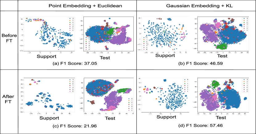
Figure 3: t-SNE visualization of support set and test set representations in a sample few-shot task in OntoNotes tag extension. We show both support and test set representation here before and after finetuning. Prior to finetuning, (a) contrastive learner with point embedding and Euclidean distance objective gives intermixed class representations; (b) Gaussian Embedding with KL-divergenece generates clusters for different unseen classes. After finetuning, (c) point embedding overfits the support examples which further intermingles different class examples; (d) Gaussian Embedding with KL-divergence cleans up the clusters offering better separation between different classes, which results in higher F1-score.

Appendix C t-SNE Visualization: Point Embedding vs. Gaussian Embedding

Figure 3 offers a deep dive into how Gaussian Embedding improves generalization and takes better advantage of few shot support set for target domain adaptation. Here we compare the t-SNE visualization of support set and test set of a sample few-shot scenario in OntoNotes tag set extension task. In Figure 3 (a) we can see that point embedding paired with Euclidean distance metric has suboptimal clustering pattern in both support and test sets. In fact, the support examples in different classes are intermixed implying poor generalization. When the point embedding model is finetuned with the support set (Figure 3 (c)), Euclidean distance aggressively optimizes them and tries to force the same class support examples to collapse into essentially a single point representation. In other words, the model quickly overfits the small support data which in fact hurts model performance. In comparsion, Gaussian Embedding offers a better t-SNE representation prior to and after finetuning. Figure 3 (b) shows the representation of support and test sets prior to finetuning with Gaussian Embedding paired with KL-divergence. In both support and test sets, we observe different class samples mostly clustered together. This indicates that even before finetuning it shows good generalization to unseen classes. While finetuning, the KL-divergence optimization objective maintains the class distribution letting the model generate separate support clusters (Figure 3(d)). After finetuning, the clusters get cleaner offering even better separation between different class clusters, which is also reflected in the performance uplift of the model.

Model	1-shot				5-shot
	Group A	Group B	Group C	Avg.	Group A	Group B	Group C	Avg.
Point Embedding + Cosine	7.73	11.27	15.57	11.52	17.33	30.08	22.51	23.31
Point Embedding + Euclidean	14.96	13.67	11.12	13.25	25.35	41.56	43.11	36.67
Gaussian Embedding + KL-div.	32.2	30.9	32.9	32.0	51.2	55.9	61.5	56.2

Table 8: OntoNotes Tag Set extension mean-F1 score comparison between Point Embedding (with Euclidean distance and cosine similarity) and Gaussian Embedding (KL-divergence).

Appendix D Comparison of Different Training Objectives

Table 8 compares the performance of Gaussian Embedding (KL-divergence) with that of point embedding (Euclidean distance of cosine similarity) in OntoNotes tag extension task. Since Gaussian Embedding utilizes $l$ dimensional mean and $l$ dimensional diagonal covariance matrix, for a fair comaparison we show the results for $2l$ dimensional point embedding. As discussed in Section 5.2, Gaussian Embedding with KL-divergence objective largely outperforms point embedding irrespective of distance metric used.

Appendix E Embedding Quality: Before vs. After Projection

	Before Projection	After Projection
1-shot	32.17	29.21
5-shot	51.19	49.78

Table 9: Comparison of F1-Scores on OntoNotes Group A before and after the projection layer of CONTaiNER

As explained in Section 3.4, the representation before the projection layer contains more information than that of after. In Table 9, we compare the performance of representations before and after the Gaussian projection layer. From the results it is evident that, representation before the projection indeed achieves higher performance, which also supports the findings of Chen et al. (2020). This is because the representation after the projection head is directly adjacent to the contrastive objective, which causes information loss in this layer. Consequently, the representation before projection achieves better performance.

Appendix F NER Prediction Examples

Table LABEL:tab:case_study demonstrates some predictions with CONTaiNER and StructShot using PERSON, DATE, MONEY, LOC, FAC, PRODUCT as target few-shot entities while being trained on all other entity types in OntoNotes dataset. A quick look at these qualitative examples reveal that StructShot often fails to distinguish between non-entity and entity tokens. Moreover, it also misclassifies non-entity tokens as one of the target classes. CONTaiNER on the other hand has lower misclassifications and better entity detection indicating its stability and higher performance.

Table 10: NER Prediction Examples from OntoNotes with PERSON, DATE, MONEY, LOC, FAC,PRODUCT as target few-shot entities

Gold	CONTaiNER	StructShot
BMEC general director Dr. ${\color[rgb]{0,0,1}\text{Johnsee Lee}}_{{\color[rgb]{0,1,0}PER}}$ says that the ITRI ’s ${\color[rgb]{0,0,1}\text{four-year}}_{{\color[rgb]{0,1,0}DATE}}$ R&D program in biochip applications and technology is now in its ${\color[rgb]{0,0,1}\text{second year}}_{{\color[rgb]{0,1,0}DATE}}$.	BMEC general director Dr. ${\color[rgb]{0,0,1}\text{Johnsee Lee}}_{{\color[rgb]{0,1,0}PER}}$ says that the ITRI ’s ${\color[rgb]{0,0,1}\text{four-year}}_{{\color[rgb]{0,1,0}DATE}}$ R&D program in biochip applications and technology is now in its ${\color[rgb]{0,0,1}\text{second year}}_{{\color[rgb]{0,1,0}DATE}}$.	BMEC general director Dr. ${\color[rgb]{0,0,1}\text{Johnsee Lee}}_{{\color[rgb]{0,1,0}PER}}$ says that the ITRI ’s ${\color[rgb]{0,0,1}\text{four-year}}_{{\color[rgb]{0,1,0}DATE}}$ R&D program in biochip applications and technology is now in its second year.
DR. Chip Bio-technology was set up in ${\color[rgb]{0,0,1}\text{September 1998}}_{{\color[rgb]{0,1,0}DATE}}$.	DR. Chip Bio-technology was set up in ${\color[rgb]{0,0,1}\text{September 1998}}_{{\color[rgb]{0,1,0}DATE}}$.	${\color[rgb]{0,0,1}\text{DR. Chip Bio-technology}}_{{\color[rgb]{0,1,0}PRODUCT}}$ was set up in September 1998.
${\color[rgb]{0,0,1}\text{Wang Shin - hwan}}_{{\color[rgb]{0,1,0}PER}}$ notes that traditional bacterial and viral cultures take seven to ten days to prepare , and even with the newer molecular biology testing techniques it takes ${\color[rgb]{0,0,1}\text{three days}}_{{\color[rgb]{0,1,0}DATE}}$ to get a result .	${\color[rgb]{0,0,1}\text{Wang Shin}}_{{\color[rgb]{0,1,0}PER}}$ - hwan notes that traditional bacterial and viral cultures take ${\color[rgb]{0,0,1}\text{seven to ten days}}_{{\color[rgb]{0,1,0}DATE}}$ to prepare , and even with the newer molecular biology testing techniques it takes ${\color[rgb]{0,0,1}\text{three days}}_{{\color[rgb]{0,1,0}DATE}}$ to get a result .	Wang Shin - hwan notes that traditional bacterial and viral cultures take ${\color[rgb]{0,0,1}\text{seven to ten days}}_{{\color[rgb]{0,1,0}DATE}}$ to prepare , and even with the newer molecular biology testing techniques it takes ${\color[rgb]{0,0,1}\text{three days}}_{{\color[rgb]{0,1,0}DATE}}$ to get a result .
Research program director ${\color[rgb]{0,0,1}\text{Pan Chao - chi}}_{{\color[rgb]{0,1,0}PER}}$ states that at present they are actively developing a " fever chip " with a wide range of applications .	Research program director ${\color[rgb]{0,0,1}\text{Pan}}_{{\color[rgb]{0,1,0}PER}}$ Chao - chi states that at ${\color[rgb]{0,0,1}\text{present}}_{{\color[rgb]{0,1,0}DATE}}$ they are actively developing a " fever chip " with a wide range of applications .	Research program director ${\color[rgb]{0,0,1}\text{Pan}}_{{\color[rgb]{0,1,0}PER}}$ Chao - chi states that at present they are actively developing a " fever chip " with a wide range of applications .
Pan explains that in clinical practice , the causes of fever are difficult to quickly diagnose .	${\color[rgb]{0,0,1}\text{Pan}}_{{\color[rgb]{0,1,0}PER}}$ explains that in clinical practice , the causes of fever are difficult to quickly diagnose .	Pan explains that in clinical practice , the causes of fever are difficult to quickly diagnose .
${\color[rgb]{0,0,1}\text{Jerry Huang}}_{{\color[rgb]{0,1,0}PER}}$, executive vice president of U - Vision Biotech , reveals that U - Vision , which was set up in ${\color[rgb]{0,0,1}\text{September 1999}}_{{\color[rgb]{0,1,0}DATE}}$, has signed a contract with the US company Zen - Bio to jointly develop human adipocyte cDNA microarray chips .	${\color[rgb]{0,0,1}\text{Jerry Huang}}_{{\color[rgb]{0,1,0}PER}}$, executive vice president of U - Vision Biotech , reveals that U - Vision , which was set up in ${\color[rgb]{0,0,1}\text{September 1999}}_{{\color[rgb]{0,1,0}DATE}}$, has signed a contract with the US company Zen - Bio to jointly develop human adipocyte cDNA microarray chips .	Jerry Huang , executive vice president of U - Vision Biotech , reveals that U - Vision , which was set up in September 1999 , has signed a contract with the US company Zen - Bio to jointly develop human adipocyte cDNA microarray chips.
${\color[rgb]{0,0,1}\text{Huang}}_{{\color[rgb]{0,1,0}PER}}$ states that research in ${\color[rgb]{0,0,1}\text{recent years}}_{{\color[rgb]{0,1,0}DATE}}$has revealed that adipocytes -LR fat cells -RR are active regulators of the energy balance in the body , and play an important role in disorders such as obesity , diabetes , osteoporosis and cardiovascular disease .	${\color[rgb]{0,0,1}\text{Huang}}_{{\color[rgb]{0,1,0}PER}}$ states that research in ${\color[rgb]{0,0,1}\text{recent years}}_{{\color[rgb]{0,1,0}DATE}}$has revealed that adipocytes -LR fat cells -RR are active regulators of the energy balance in the body , and play an important role in disorders such as obesity , diabetes , osteoporosis and cardiovascular disease .	Huang states that research in recent years has revealed that adipocytes -LR fat cells -RR are active regulators of the energy balance in the body , and play an important role in disorders such as obesity , diabetes , osteoporosis and cardiovascular disease .
Maybe a ${\color[rgb]{0,0,1}\text{30 year old}}_{{\color[rgb]{0,1,0}DATE}}$ man & a ${\color[rgb]{0,0,1}\text{15 year old}}_{{\color[rgb]{0,1,0}DATE}}$boy doesn’t qualify .	Maybe a 30 year old man & a 15 year old boy doesn’t qualify .	Maybe a ${\color[rgb]{0,0,1}\text{30 year old}}_{{\color[rgb]{0,1,0}DATE}}$ man & a ${\color[rgb]{0,0,1}\text{15 year old}}_{{\color[rgb]{0,1,0}DATE}}$boy doesn’t qualify .
After ${\color[rgb]{0,0,1}\text{Tom DeLay}}_{{\color[rgb]{0,1,0}PER}}$ was zapped, ${\color[rgb]{0,0,1}\text{Charles Colson}}_{{\color[rgb]{0,1,0}PER}}$ became ${\color[rgb]{0,0,1}\text{DeLay}}_{{\color[rgb]{0,1,0}PER}}$’s personal guru.	After ${\color[rgb]{0,0,1}\text{Tom DeLay}}_{{\color[rgb]{0,1,0}PER}}$ was zapped, ${\color[rgb]{0,0,1}\text{Charles Colson}}_{{\color[rgb]{0,1,0}PER}}$ became DeLay’s personal guru.	After Tom DeLay was zapped, ${\color[rgb]{0,0,1}\text{Charles Colson}}_{{\color[rgb]{0,1,0}PER}}$ became DeLay’s personal guru.
She does not sit still or lay still for you to change her ${\color[rgb]{0,0,1}\text{Pampers}}_{{\color[rgb]{0,1,0}PRODUCT}}$.	She does not sit still or lay still for you to change her ${\color[rgb]{0,0,1}\text{Pampers}}_{{\color[rgb]{0,1,0}PRODUCT}}$.	She does not sit still or lay still for you to change her ${\color[rgb]{0,0,1}\text{Pampers}}_{{\color[rgb]{0,1,0}PRODUCT}}$.
Russian and Norwegian divers searched the fourth compartment of the wrecked submarine ${\color[rgb]{0,0,1}\text{Kursk}}_{{\color[rgb]{0,1,0}PRODUCT}}$, ${\color[rgb]{0,0,1}\text{Sunday}}_{{\color[rgb]{0,1,0}DATE}}$, but they found too much damage to proceed with the task of recovering bodies .	Russian and Norwegian divers searched the fourth compartment of the wrecked submarine ${\color[rgb]{0,0,1}\text{Kursk}}_{{\color[rgb]{0,1,0}PRODUCT}}$, ${\color[rgb]{0,0,1}\text{Sunday}}_{{\color[rgb]{0,1,0}DATE}}$, but they found too much damage to proceed with the task of recovering bodies .	Russian and Norwegian divers searched the fourth compartment of the wrecked submarine Kursk, ${\color[rgb]{0,0,1}\text{Sunday}}_{{\color[rgb]{0,1,0}DATE}}$, but they found too much damage to proceed with the task of recovering bodies .
${\color[rgb]{0,0,1}\text{Zinni}}_{{\color[rgb]{0,1,0}PER}}$ testifying after the attack on ${\color[rgb]{0,0,1}\text{the ``USS Cole''}}_{{\color[rgb]{0,1,0}PRODUCT}}$ – Aden never had a specific terrorist threat .	${\color[rgb]{0,0,1}\text{Zinni}}_{{\color[rgb]{0,1,0}PER}}$ testifying after the attack on ${\color[rgb]{0,0,1}\text{the ``USS Cole''}}_{{\color[rgb]{0,1,0}PRODUCT}}$ – Aden never had a specific terrorist threat .	Zinni testifying after the attack on ${\color[rgb]{0,0,1}\text{the ``USS Cole''}}_{{\color[rgb]{0,1,0}PRODUCT}}$ – Aden never had a specific terrorist threat .
Today , the enterovirus chip is in the testing phase , and DR. Chip is collaborating with Taipei Veterans General Hospital to obtain samples with which to establish the accuracy of the chip .	${\color[rgb]{0,0,1}\text{Today}}_{{\color[rgb]{0,1,0}DATE}}$, the enterovirus chip is in the testing phase, and ${\color[rgb]{0,0,1}\text{DR. Chip}}_{{\color[rgb]{0,1,0}PRODUCT}}$ is collaborating with ${\color[rgb]{0,0,1}\text{Taipei Veterans General Hospital}}_{{\color[rgb]{0,1,0}FAC}}$ to obtain samples with which to establish the accuracy of the chip .	${\color[rgb]{0,0,1}\text{Today}}_{{\color[rgb]{0,1,0}DATE}}$, the enterovirus chip is in the testing phase, and ${\color[rgb]{0,0,1}\text{DR. Chip}}_{{\color[rgb]{0,1,0}PRODUCT}}$ is collaborating with Taipei Veterans General Hospital to obtain samples with which to establish the accuracy of the chip .
And I think perhaps no one more surprised than some of the people running those firms on ${\color[rgb]{0,0,1}\text{Wall Street}}_{{\color[rgb]{0,1,0}FAC}}$.	I think perhaps no one more surprised than some of the people running those firms on ${\color[rgb]{0,0,1}\text{Wall Street}}_{{\color[rgb]{0,1,0}FAC}}$.	I think perhaps no one more surprised than some of the people running those firms on Wall Street.
We’re all getting , this news in from the speech that the Homeland Security Secretary ${\color[rgb]{0,0,1}\text{Tom Ridge}}_{{\color[rgb]{0,1,0}PER}}$ is expected to be delivering at the international press club around 1:00 Eastern at the top of the hour .	We’re all getting , this news in from the speech that the Homeland Security Secretary ${\color[rgb]{0,0,1}\text{Tom Ridge}}_{{\color[rgb]{0,1,0}PER}}$ is expected to be delivering at the international press club around 1:00 Eastern at the top of the hour .	We’re all getting , this news in from the speech that the Homeland Security Secretary ${\color[rgb]{0,0,1}\text{Tom Ridge}}_{{\color[rgb]{0,1,0}PER}}$ is expected to be delivering at the international press ${\color[rgb]{0,0,1}\text{club}}_{{\color[rgb]{0,1,0}FAC}}$ around 1:00 Eastern at the top of the hour .
${\color[rgb]{0,0,1}\text{Yesterday}}_{{\color[rgb]{0,1,0}DATE}}$ American pilots mechanics approved their share ${\color[rgb]{0,0,1}\text{\$ 1.8 billion}}_{{\color[rgb]{0,1,0}MONEY}}$ in labor concession .	${\color[rgb]{0,0,1}\text{Yesterday}}_{{\color[rgb]{0,1,0}DATE}}$ American pilots mechanics approved their share ${\color[rgb]{0,0,1}\text{\$ 1.8 billion}}_{{\color[rgb]{0,1,0}MONEY}}$ in labor concession .	Yesterday American pilots mechanics approved their share $ 1.8 billion in labor concession .

References

- Athiwaratkun and Wilson (2018) Ben Athiwaratkun and Andrew Gordon Wilson. 2018. Hierarchical density order embeddings. arXiv preprint arXiv:1804.09843.
- Bao et al. (2020) Yujia Bao, Menghua Wu, Shiyu Chang, and Regina Barzilay. 2020. Few-shot text classification with distributional signatures. In ICLR.
- Bojchevski and Günnemann (2017) Aleksandar Bojchevski and Stephan Günnemann. 2017. Deep gaussian embedding of graphs: Unsupervised inductive learning via ranking. arXiv preprint arXiv:1707.03815.
- Chen et al. (2020) Ting Chen, Simon Kornblith, Mohammad Norouzi, and Geoffrey Hinton. 2020. A simple framework for contrastive learning of visual representations. In ICML.
- Cui et al. (2021) Leyang Cui, Yu Wu, Jian Liu, Sen Yang, and Yue Zhang. 2021. Template-based named entity recognition using bart. arXiv preprint arXiv:2106.01760.
- Derczynski et al. (2017) Leon Derczynski, Eric Nichols, Marieke van Erp, and Nut Limsopatham. 2017. Results of the wnut2017 shared task on novel and emerging entity recognition. In Proceedings of the 3rd Workshop on Noisy User-generated Text, pages 140–147.
- Devlin et al. (2018) Jacob Devlin, Ming-Wei Chang, Kenton Lee, and Kristina Toutanova. 2018. Bert: Pre-training of deep bidirectional transformers for language understanding. arXiv preprint arXiv:1810.04805.
- Ding et al. (2021) Ning Ding, Guangwei Xu, Yulin Chen, Xiaobin Wang, Xu Han, Pengjun Xie, Haitao Zheng, and Zhiyuan Liu. 2021. Few-nerd: A few-shot named entity recognition dataset. In Proceedings of the 59th Annual Meeting of the Association for Computational Linguistics and the 11th International Joint Conference on Natural Language Processing (Volume 1: Long Papers), pages 3198–3213.
- Doersch and Zisserman (2017) Carl Doersch and Andrew Zisserman. 2017. Multi-task self-supervised visual learning. In Proceedings of the IEEE International Conference on Computer Vision, pages 2051–2060.
- Dosovitskiy et al. (2014) Alexey Dosovitskiy, Jost Tobias Springenberg, Martin Riedmiller, and Thomas Brox. 2014. Discriminative unsupervised feature learning with convolutional neural networks. Advances in neural information processing systems, 27:766–774.
- Fei-Fei et al. (2006) Li Fei-Fei, Rob Fergus, and Pietro Perona. 2006. One-shot learning of object categories. IEEE transactions on pattern analysis and machine intelligence, 28(4):594–611.
- Fritzler et al. (2019) Alexander Fritzler, Varvara Logacheva, and Maksim Kretov. 2019. Few-shot classification in named entity recognition task. In Proceedings of the 34th ACM/SIGAPP Symposium on Applied Computing, pages 993–1000.
- Geng et al. (2019) Ruiying Geng, Binhua Li, Yongbin Li, Xiaodan Zhu, Ping Jian, and Jian Sun. 2019. Induction networks for few-shot text classification. arXiv preprint arXiv:1902.10482.
- Ghaddar and Langlais (2017) Abbas Ghaddar and Philippe Langlais. 2017. Winer: A wikipedia annotated corpus for named entity recognition. In Proceedings of the Eighth International Joint Conference on Natural Language Processing (Volume 1: Long Papers), pages 413–422.
- Hadsell et al. (2006) Raia Hadsell, Sumit Chopra, and Yann LeCun. 2006. Dimensionality reduction by learning an invariant mapping. In 2006 IEEE Computer Society Conference on Computer Vision and Pattern Recognition (CVPR’06), volume 2, pages 1735–1742. IEEE.
- Han et al. (2018) Xu Han, Hao Zhu, Pengfei Yu, Ziyun Wang, Yuan Yao, Zhiyuan Liu, and Maosong Sun. 2018. Fewrel: A large-scale supervised few-shot relation classification dataset with state-of-the-art evaluation. arXiv preprint arXiv:1810.10147.
- Hou et al. (2020) Yutai Hou, Wanxiang Che, Yongkui Lai, Zhihan Zhou, Yijia Liu, Han Liu, and Ting Liu. 2020. Few-shot slot tagging with collapsed dependency transfer and label-enhanced task-adaptive projection network. arXiv preprint arXiv:2006.05702.
- Huang et al. (2020) Jiaxin Huang, Chunyuan Li, Krishan Subudhi, Damien Jose, Shobana Balakrishnan, Weizhu Chen, Baolin Peng, Jianfeng Gao, and Jiawei Han. 2020. Few-shot named entity recognition: A comprehensive study. arXiv preprint arXiv:2012.14978.
- Huang et al. (2015) Zhiheng Huang, Wei Xu, and Kai Yu. 2015. Bidirectional lstm-crf models for sequence tagging. arXiv preprint arXiv:1508.01991.
- Khosla et al. (2020) Prannay Khosla, Piotr Teterwak, Chen Wang, Aaron Sarna, Yonglong Tian, Phillip Isola, Aaron Maschinot, Ce Liu, and Dilip Krishnan. 2020. Supervised contrastive learning. arXiv preprint arXiv:2004.11362.
- Lafferty et al. (2001) John Lafferty, Andrew McCallum, and Fernando CN Pereira. 2001. Conditional random fields: Probabilistic models for segmenting and labeling sequence data. In ICML.
- Lake et al. (2011) Brenden Lake, Ruslan Salakhutdinov, Jason Gross, and Joshua Tenenbaum. 2011. One shot learning of simple visual concepts. In Proceedings of the annual meeting of the cognitive science society.
- Lample et al. (2016) Guillaume Lample, Miguel Ballesteros, Sandeep Subramanian, Kazuya Kawakami, and Chris Dyer. 2016. Neural architectures for named entity recognition. arXiv preprint arXiv:1603.01360.
- Ma and Hovy (2016) Xuezhe Ma and Eduard Hovy. 2016. End-to-end sequence labeling via bi-directional lstm-cnns-crf. arXiv preprint arXiv:1603.01354.
- Misra and Maaten (2020) Ishan Misra and Laurens van der Maaten. 2020. Self-supervised learning of pretext-invariant representations. In Proceedings of the IEEE/CVF Conference on Computer Vision and Pattern Recognition, pages 6707–6717.
- Perez et al. (2021) Ethan Perez, Douwe Kiela, and Kyunghyun Cho. 2021. True few-shot learning with language models. arXiv preprint arXiv:2105.11447.
- Peters et al. (2018) Matthew E Peters, Mark Neumann, Mohit Iyyer, Matt Gardner, Christopher Clark, Kenton Lee, and Luke Zettlemoyer. 2018. Deep contextualized word representations. arXiv preprint arXiv:1802.05365.
- Qian et al. (2021) Chen Qian, Fuli Feng, Lijie Wen, and Tat-Seng Chua. 2021. Conceptualized and contextualized gaussian embedding. In Proceedings of the AAAI Conference on Artificial Intelligence, volume 35, pages 13683–13691.
- Sang and De Meulder (2003) Erik F Sang and Fien De Meulder. 2003. Introduction to the conll-2003 shared task: Language-independent named entity recognition. arXiv preprint cs/0306050.
- Snell et al. (2017) Jake Snell, Kevin Swersky, and Richard S Zemel. 2017. Prototypical networks for few-shot learning. arXiv preprint arXiv:1703.05175.
- Stubbs and Uzuner (2015) Amber Stubbs and Özlem Uzuner. 2015. Annotating longitudinal clinical narratives for de-identification: The 2014 i2b2/uthealth corpus. Journal of biomedical informatics, 58:S20–S29.