Non-smooth Bayesian Optimization in Tuning Problems

Abstract

Building surrogate models is one common approach when we attempt to learn unknown black-box functions. Bayesian optimization provides a framework which allows us to build surrogate models based on sequential samples drawn from the function and find the optimum. Tuning algorithmic parameters to optimize the performance of large, complicated “ black-box” application codes is a specific important application, which aims at finding the optima of black-box functions. Within the Bayesian optimization framework, the Gaussian process model produces smooth or continuous sample paths. However, the black-box function in the tuning problem is often non-smooth. This difficult tuning problem is worsened by the fact that we usually have limited sequential samples from the black-box function. Motivated by these issues encountered in tuning, we propose a novel additive Gaussian process model called clustered Gaussian process (cGP), where the additive components are induced by clustering. In the examples we studied, the performance can be improved by as much as 90% among repetitive experiments. By using this surrogate model, we want to capture the non-smoothness of the black-box function. In addition to an algorithm for constructing this model, we also apply the model to several artificial and real applications to evaluate it.

Keywords: Bayesian optimization, surrogate modeling, additive Gaussian models.

1 Introduction

As an introduction, we briefly review the recent literature on Bayesian optimization and identify the problem caused by non-smoothness in tuning scenarios in subsection 1.1. The follow-up subsections 1.2 and 1.3 describe the non-smoothness phenomena and focus on one specific kind of non-smoothness.

1.1 Problems and Challenges

Suppose that we have a scalar function $f$ whose expression we do not know, but we can draw noisy samples in the form of pairs $(\bm{x},y)=(\bm{x},f(\bm{x}))$ from function $f$, i.e., we consider a noisy optimization model. The methodology we present in the current paper focuses on univariate functions and could be extended to multivariate functions, but this remains a possible future work.

• When it is easy (or cheap) to evaluate this function at any point of its domain, the default strategy is to use an exhaustive grid search of $\bm{x}$ to find its optimum.

• When it is difficult (or expensive) to evaluate this function at some points of its domain, one strategy is to use a relatively cheap surrogate model to approximate the black-box function.

The general tuning problem is to find the maximum or minimum of such a function $f$ based on (noisy) samples sequentially drawn from the function. This function with an unknown expression is usually called a black-box function. An analytic solution for the optimum of $f$ is usually impossible; even if the analytic expression of the function is known, the analytic optimum could be not tractable or expensive to evaluate. In various scenarios, we need to solve this kind of black-box optimization problem (Müller and Day, 2019; Gramacy, 2020).

Following common strategies, a surrogate model $g$ is proposed to model the underlying black-box function $f$. The chosen surrogate model $g$ needs to be easier to evaluate and approximate the black-box function $f$ reasonably well. This strategy usually works well for smooth functions.

Bayesian optimization provides a surrogate modeling optimization framework that allows us to model and optimize these black-box functions using sequential sampling (Booker et al., 1999; Snoek et al., 2012; Shahriari et al., 2016; Gramacy, 2020). In practice, we sequentially draw expensive samples from the black-box function $f$ and update the surrogate model $g$ with the samples drawn using Bayes’ theorem. If the surrogate model $g$ approximates the black-box function $f$ sufficiently well, we will expect that the optimum obtained from the surrogate model is sufficiently close the true optimum $\max_{\bm{x}}f(\bm{x})$ of the black-box function. That is, if we can ensure $g\approx f$, then their optima can be off by a max error at most $\|f-g\|_{\infty}$. Gaussian process (GP) modeling is a predominantly popular choice for building surrogate models $g$ in Bayesian optimization. The most obvious reason for this choice of GP surrogate model is its convenient conjugacy in Bayes’ theorem and its well-studied covariance dependence structures (Rasmussen and Williams, 2006; Shah et al., 2014). And the sequential sampling scheme can be guided by maximizing the acquisition function within the Bayesian framework (Gramacy and Polson, 2010; Gramacy and Ludkovski, 2015). We summarize the recent progress of the existing problems and challenges pointed out by Shahriari et al. (2016), where a comprehensive introduction to Bayesian optimization is given.

• Constrained Bayesian optimization. A constrained Bayesian optimization problem considers a domain which is not a full space. Notably, Müller and Day (2019) propose grid-based searches for optimization with hidden constraints, following a line of research tackling mixed integer (Holmström et al., 2008), unknown (Gramacy and Lee, 2011) and noisy constraints (Letham et al., 2019).

• Cost sensitivity. The problem of cost sensitivity arises in computer experiment applications and can be incorporated in the Bayesian optimization context (Brochu et al., 2010). Lee et al. (2020) recently propose a cost-aware metric, in combination with cost-effective pilot samples.

• High-dimensional problems. Most Bayesian optimization models focus on low-dimensional domains (Gramacy and Polson, 2010; Snoek et al., 2012). Chen et al. (2012) propose a two-stage strategy to fit high-dimensional GP surrogate models by dropping some dimensions. However, when there are insufficient samples, high-dimensional over-parameterized surrogate models may suffer.

• Multi-task. Multi-task optimization aims at approximating multiple responses simultaneously. Following Williams et al. (2007), Swersky et al. (2013) provide a unified framework for multiple-output GP surrogates. Additive GP surrogate models are designed for multi-fidelity applications with approximations (Kandasamy et al., 2017) or generalized acquisition functions (Song et al., 2019).

• Freeze-thaw. The freeze-thaw strategy considers a subcategory of GP surrogate models where inner loops of iterative optimization are needed (Swersky et al., 2014). This approach has been incorporated into the iterative learning framework (Nguyen et al., 2020). Meanwhile, the criticisms of freeze-thaw approach are mostly based on its complicated implementation and highly application-dependent nature (Dai et al., 2019).

The main application that motivates the current paper is the tuning problem in computational science. In the tuning problem, an expensive black-box cost function $f$, typically the running time of a complicated simulation, with a moderate dimensional variable $\bm{x}$, typically a set of algorithmic tuning parameters, needs to be optimized with a limited sequential sample size. In addition, another important challenge is the potential non-smoothness in the black-box cost function. Tuning becomes more crucial in large-scale computational applications, and surrogate modeling with GP becomes an effective approach (Sid-Lakhdar et al., 2019). The GP modeling will produce continuous sample paths (Cramér and Leadbetter, 2013), but has difficulty in capturing potential non-smoothness (e.g., jumps in black-box performance functions) in the black-box function. This feature of GP surrogates makes it difficult to model cost functions in tuning problems, whose black-box functions often come with potential discontinuities.

As a motivation, we consider a univariate cost function that arises in a specific tuning problem. In a matrix multiplication problem $AB=C$, the practice of blocking large matrices $A,B,C$ and performing block-wise multiplication is done to improve the computational performance (Hong and Kung, 1981; Blackford et al., 2002; Bilmes et al., 1997; Whaley et al., 2001; Zee et al., 2016). The black-box function $f$ is the measured computational speed ($\mathtt{Mflops/s}$) of this matrix multiplication operation (matmul), which is determined by the efficiency of the block matrix multiplication algorithm along with the potential measurement noise. The tuning parameter in this problem is the block size for these blocked matrices. On one hand, we can increase the block size in order to reduce the amount of data movement between fast and slow caches to speed up the multiplication. On the other hand, since the processor cache is finite, when the matrix block is too large to fit into the cache, it would cause cache misses and hence a sudden drop in the computational performance.

Hong and Kung (1981) use a pebble game model on an acyclic directed graph to derive an analytical optimal bound for cost function of this application. The optimal block size is machine dependent since processor cache sizes can differ, and also depends on the structure of the innermost loops. We want to “tune” the optimal block size to attain the fastest matrix multiplication. This motivating example drives us to consider an optimization problem where the black-box function $f:\mathbb{Z}_{+}\rightarrow\mathbb{R}^{1}$ has potential non-smoothness with respect to the block size to be tuned (and where there is no explicit way to compute the optimal block size).

This application of matmul will be our example showing why different partitions may arise naturally in the context of tuning. We also provide multiple synthetic and real-world tuning examples like SuperLU (Yamazaki and Li, 2012) showing the improvement when partitioning is well utilized in the optimization. We want to optimize a non-smooth black-box function with a variant of GP surrogate, which leads to our proposal below.

1.2 Non-smoothness caused by the domain

The black-box function $f$ may be defined on a discrete domain like $\mathbb{Z}^{d}$ instead of $\mathbb{R}^{d}$. This kind of problem is known as a problem with integer constraints (Müller and Day, 2019; Garrido-Merchán and Hernández-Lobato, 2020). Furthermore, if only some of the input dimensions are discrete and the black-box function is defined as $f:\mathbb{Z}^{d-r}\times\mathbb{R}^{r}\rightarrow\mathbb{R}^{1}$, then the problem has mixed-integer constraints. This kind of problem could be addressed with different grid-based search methods and generalized into multiple-objective situations within the Bayesian optimization framework (Holmström et al., 2008; Gramacy and Lee, 2011).

Usually, a GP surrogate model will be assumed to be fitted on a continuous input domain. In the situation where the input domain is (partially) discrete, a common practice is to discretize the continuous input variables of a (univariate) GP surrogate model $g:\mathbb{R}^{d}\rightarrow\mathbb{R}^{1}$ whose mean function approximates $f$ with uncertainty quantification, while the handling of categorical or integer variables in Bayesian optimism is ongoing research (Ru et al., 2020). However, if we have a (piecewise) continuous black-box function $f:\mathbb{R}^{d}\rightarrow\mathbb{R}^{1}$, this simple discretization without appropriate adjustment in the covariance structure of GP surrogate model may yield incorrect results (Garrido-Merchán and Hernández-Lobato, 2020). We mainly focus on another kind of non-smoothness in the next section – the non-smoothness in the black-box function $f$ on a continuous domain.

1.3 Non-smoothness in the black-box function

In this paper, we consider the non-smoothness of the function $f$ of the following two types, where we assume the function domain is $\mathbb{R}^{d}$.

Example 1

For example, the function $f_{1}:\mathbb{R}^{1}\rightarrow\mathbb{R}^{1}$

$$f_{1}(x)=\begin{cases}-x+1&x<0\\ x^{2}&x\geq 0\end{cases},$$ (1)

defined on $\mathbb{R}^{1}$ is a piecewise continuous function. The function $f_{1}$ is not smooth and has a “jump” at the point $x=0$ from 1 to 0 with minimum $0$ reached at $0$.

Other than the non-smoothness caused by “jumps”, another kind of non-smoothness in the black-box function is caused by discontinuous derivatives.

Example 2

For example, the function $f_{2}:\mathbb{R}^{2}\rightarrow\mathbb{R}^{1}$

$$f_{2}(\bm{x})=\begin{cases}(\|\bm{x}\|-1)&\|\bm{x}\|>1\\ (\|\bm{x}\|-1)^{4}&\|\bm{x}\|\leq 1\end{cases},$$ (2)

has support $\mathbb{R}^{2}$ and a discontinuous derivative on the circle $S^{1}:\|\bm{x}\|=1$, where it attains its minimum value of 0. In special cases, such non-smoothness can be captured asymptotically with sufficient samples (Luo et al., 2020a).

Although different choices of covariance kernels would adjust the smoothness of the surrogate model $g$, a GP surrogate would not accurately model “jumps”. Here is one example of the effect of non-smooth black-box functions. Since there could be more than one parameter that specifies the kernel, we use $\bm{\kappa}$ to denote all kernel parameters for kernel $K=K_{\bm{\kappa}}$ below for brevity.

In Figure 1.1, we show the fitted mean function of GP and piecewise GP surrogate models (with a deterministic partition) in the unrealistic best-case situation where we know the exact location of the discontinuity. All models are based on the same 10 pilot samples drawn from equally spaced locations on $[-1,1]$ from $f_{1}$ above, with Gaussian noise with variance $0.01$. We provide surrogate fits with Matérn covariance kernels with parameters $\nu=1/2,3/2,5/2,\infty$, which adjusts the smoothness of the GP surrogate.

For the simple GP surrogate models displayed in the first row, near the non-smooth point $x=0$, we see a lack-of-fit between the black-box function and the fitted mean function from the surrogate models. We also fit a piecewise GP surrogate model $g=g_{1}+g_{2}$ where $g_{1}$ and $g_{2}$ are supported on $(-\infty,0]$ and $[0,+\infty)$ respectively. From the second row of the figure, we can see that this additive approach captures the non-smoothness that occurs at $x=0$, and the minimum obtained from $g$ is closer to the true minimum at 0 for a single GP with any kernel. An important observation is that an appropriate partition of the input domain helps the surrogate model capture the non-smoothness, compared to simple GP surrogate models.

The non-smoothness in $f_{2}$ is caused by discontinuous derivatives, and the non-smoothness in $f_{1}$ is a “jump”. This terminology is more general than the “change-point” and “change-surface”, which are usually restricted to specific dimensions. The presence of non-smoothness in the black-box function will cause GP surrogate models $g$ to be mis-specified, and have a underlying lack-of-fit to the black-box function $f$. The existence of non-smoothness in $f$ presents challenges to the optimization since the optima may no longer be close to the true optimum when the black-box functions are non-smooth as shown in Figure 1.1.

On one hand, mathematically, the non-smoothness should be considered in the context of continuity of functions. However, the mathematical definition requires arbitrarily many points to characterize discontinuities.

On the other hand, in the surrogate modeling context, we only take finitely many sample points. Therefore, we consider those points $x_{2}$ near a (fixed) point $x_{1}$ at which the finite difference $|f(x_{1})-f(x_{2})|/\|x_{1}-x_{2}\|$ exceeds a certain threshold to be “non-smooth” but those points where the finite difference ratio falls below certain threshold to be “smooth”. This is a proxy for the formal mathematical concept. Such a consideration motivates our later construction where we use $(x,\xi y)$ as the clustering criterion in our algorithm, with a factor $\xi$ for threshold adjustment. Detailed discussions are delayed to section 2.3.

This conflict between mathematical and modeled non-smoothness cannot be resolved without high-order derivative modeling (e.g., Solak et al. (2003)). One solution is to put yet another GP surrogate to model first-order derivatives and then use that as a criterion for clustering. This scheme can be generalized to higher order derivatives, but we leave this as future work.

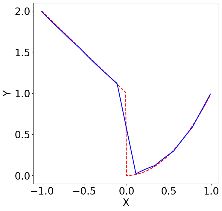
$\nu=1/2$ $\nu=3/2$ $\nu=5/2$ $\nu=\infty$ GP additive GP (with 2 components supported on $(-\infty,0]$ and $[0,+\infty)$ respectively)

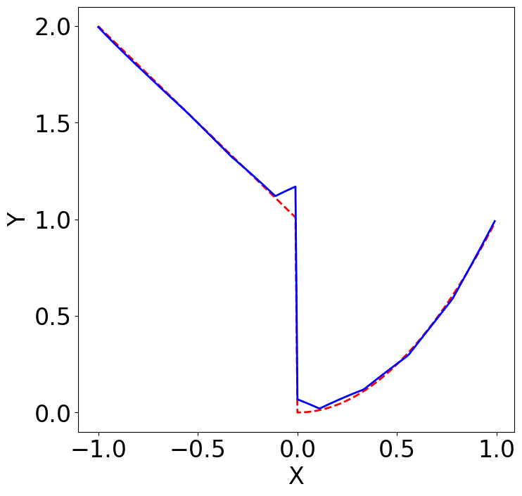
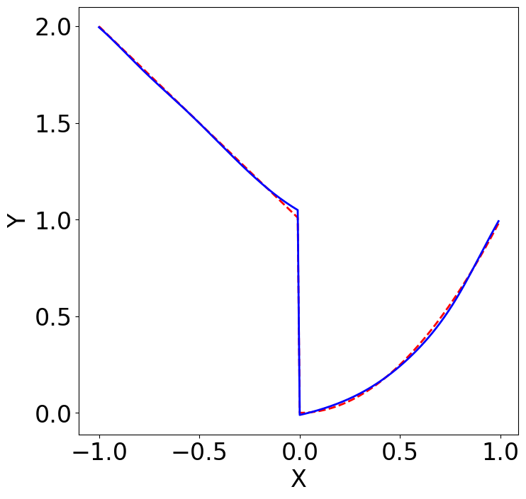
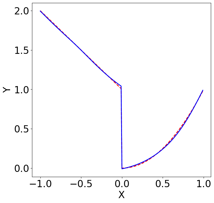
Figure 1.1: Mean function extracted from the fitted GP (first row) and piecewise GP (second row, with components supported at $(-\infty,0]$ and $[0,+\infty)$ respectively) surrogate model with $10$ equally spaced samples on $[-1,1]$ from $f_{1}$. The blue solid line is the fitted surrogate mean function and the red dashed line is the true function $f_{1}$.

Formally, we have a definition of non-smoothness of a function $f$, which captures both jumps and discontinuous derivatives:

Definition 1

(Non-smoothness) Let $f$ be a function of variable $\bm{x}\in\mathbb{R}^{d}$, we define a non-smooth point $\bm{x}_{0}$ of $f$ to be such a point that its first-order gradient $\nabla_{\bm{x}}f$ is either unbounded or does not exist at some point $\bm{x}$ in any open neighborhood of $\bm{x}_{0}$.

The two examples above do not have gradients at certain points of their domains due to “jumps” or different left- and right- limits. Another example is the function $f_{0}(x)=x^{3/2}\cdot\sin(1/x)$, which has a gradient 0 at $x=0$ but is not bounded near $x=0$. These kinds of non-smoothness can be observed in various black-box functions, as we shall see later.

The algorithm we introduce later does not use the definition, but we are motivating the choice of the clustering criterion $(\bm{x},\xi y)$ (for the moment $\xi=1$, and its role will be clear later) using this specific definition, which will enable the surrogate fitting to take non-smoothness into account.

1.4 Organization

We have briefly reviewed surrogate modeling and pointed out the problem of non-smoothness in the tuning context. The organization of the rest of this paper is as follows. In Section 2, we describe our methodology of building a non-smooth GP surrogate model, which we call a clustered GP (cGP) surrogate model, leveraging the partitioning scheme induced by the clustering to accommodate the potential non-smoothness. We first review relevant methods in handling non-smoothness in subsection 2.1, and 2.2. Subsection 2.3 discusses the intuition and construction of the proposed model. Section 3 provides simulated experiments with benchmark functions and analysis for the blocked matrix multiplication tuning problem we mentioned in subsection 1.1. Through these experiments, we observe that the surrogate-based optimization with cGP is better than GP while providing reasonable partitions. (For example, we gain around 5% improvement with a limited number of evaluations when tuning the widely used LU factorization application in Section 3.2.2. ) Moderately high-dimensional experiments are also provided to evaluate the proposed cGP surrogate model. The paper concludes with a discussion of the cGP surrogate model and future work in section 4.

2 Methodology

From what we described above in Definition 1 and the example in Figure 1.1, the problem of tackling non-smoothness in the form of “jumps” or “piecewise continuity” can be addressed by building a GP surrogate model with appropriately chosen additive components.

In Section 2.1, we discuss the existing GP methods that are relevant to consider non-smooth modeling. In the context of the tuning problem, we further focus on modeling a potentially non-smooth black-box function with limited sequential (and possibly noisy) samples. Then, we present our proposed method that is suitable for surrogate modeling in a high-dimensional domain with detailed algorithms in Section 2.3.

2.1 Relevant methods for non-smooth modeling

The first line of relevant research is the online change-point detection problem with GP models (Adams and MacKay, 2007; Saatçi et al., 2010). In a one-dimensional domain (e.g., a time-series), a change-point means that the function behavior is different before and after this point. The observed response could be characterized using different models. The problem involving change-point detection investigates whether and when such a change of behavior occurs. The setup of sequential sampling and inference is known as online detection, in contrast to offline detection where the samples are fixed and the inference is retrospective (Basseville and Nikiforov, 1993; Saatçi et al., 2010). Page (1954) first posed the problem of change-point detection, but not until Smith (1975) was the change-point problem studied with a Bayesian approach, and then Barry and Hartigan (1993) put the offline inference into a fully Bayesian framework. However, not until Adams and MacKay (2007) did a popular Bayesian change-point detection for online inference appear. This kind of online Bayesian change-point model relies on the one-dimensional time domain, making it hard to generalize to higher dimensions.

The second line of relevant research are the non-stationary GP models. In a broader (yet more vague) sense, another collection of research that is related to non-smooth modeling is non-stationary GP modeling, which is investigated in the context of spatial statistics (2-dimensional domain). Since people use the term stationary to refer to a specific family of GP models with covariance kernels depending only on pairwise point distance, GP models without such a covariance kernel could be referred as non-stationary. A stationary kernel (e.g., Matérn kernels) takes the form of $K_{\bm{\kappa}}(\bm{x}_{i},\bm{x}_{j})=K_{\bm{\kappa}}(\|\bm{x}_{i}-\bm{x}_{j}\|)$, while a non-stationary kernel could take the form that depends on specific locations $\bm{x}_{i},\bm{x}_{j}$ (Paciorek and Schervish, 2004). In the context of offline surrogate models, Krause and Guestrin (2007) propose a mixture model to address the non-stationarity based on a partition of the input domain provided by the user. Furthermore, Martinez-Cantin (2015) suggest that the partition weight functions consist of a local part and a global part in order to learn global local features including potential non-smoothness. In a different direction, Herlands et al. (2016) propose a model for the partition weight function to model general change-surfaces. These non-stationary kernels are usually overly parameterized, which might be a problem when there are only limited samples.

The third line of relevant research are in the context of online (non-GP) surrogate models. When the derivative information is not available, Stoyanov et al. (2017) model piecewise constant functions for cracking patterns using hierarchical grid-based methods, and generalize to piecewise polynomials in Stoyanov (2018); Fuchs and Garcke (2020). Although motivated by a similar problem, we do not see an immediate adaptation of the grid-based method into Bayesian optimization framework, which gives up the sequential sampling procedure. A simpler model that is often used in non-smoothness detection is MARS (Friedman, 1991). When the derivative information is available, Solak et al. (2003) suggested an approach to model observation derivatives using GP directly in the specific situation of a dynamic system where the generative equations are known. However, this is not the usual situation in the tuning or data analysis context.

2.2 Partitioning the input domain

The observation we made in Figure 1.1 is that, by fitting additive Gaussian components on appropriate partitions, the non-smoothness can be captured in the fitted model.

In the setting of limited samples, an overly parameterized surrogate model would not provide a good fit. There may be more model parameters than the samples and no unique fit is possible. Due to high dimensionality, grid search methods are no longer efficient and the non-smoothness or a change of behavior would require more samples to fit a surrogate model. These two challenges both urge for a parsimonious surrogate model, which is able to model the non-smoothness in an effective way. As a generalization of the piecewise GP shown in Figure 1.1, we believe a partition based GP surrogate model is a good candidate for handling non-smoothness in the tuning context, as will be explained below. With normalization of the inputs, we can assume the following without loss of generality.

Assumption. Hereafter, we assume that our input domain is a $d$-dimensional unit hypercube $H^{d}=[0,1]^{d}\subset\mathbb{R}^{d}$ ($d\geq 1$) for the simplicity of discussion. Our methodology can be modified to work for $\mathbb{R}^{d}$ and $\mathbb{Z}^{d}$.

It is natural to think that different components in such a surrogate model should be fitted over different partition regions determined by the non-smooth points. For instance, in Figure 1.1, the only non-smooth point for $f_{1}$ is $\bm{x}_{*}=0$ and its complement divides the domain $\mathbb{R}$ into $(-\infty,0]$ and $[0,+\infty)$.

As explained in Section 1.3, we are inspired by the partitioning method used for GP modeling in general. For example, a tree-like partition is utilized in order to handle non-stationarity in GP modeling (Chipman et al., 1998, 2010; Luo et al., 2020b). Furthermore, overly parameterized change-surface models (Martinez-Cantin, 2015; Herlands et al., 2016) can be perceived as partitioning the domain with the support of the weight functions using the change-surfaces. The effect of partitioning is restricting each surrogate model component to the corresponding piece of the domain, and assembling these components to obtain the overall surrogate. Existing partition-based GP models are usually for offline situations, but in our context, the partition must be able to update according to the sequential sampling.

The tuning problem brings us the following challenges. Although our main focus is to develop a novel modeling method to model non-smoothness, we will show by experiments and examples that our model can address the following challenges relatively well.

• Limited and sequential samples. For tuning problems, we need to fit a GP surrogate model with limited sequential samples. Limited and sequential samples make fitting GP surrogate models more difficult and dependent on the choice of samples in each sampling step. With limited samples, it is impossible to fit (non-stationary) models with over-parameterization.

• High-dimensional generalization. Bayesian optimization for the tuning problem usually has a natural moderately high-dimensional domain (e.g., $\mathbb{R}^{d}$ with $d>2$), but it is not immediately clear how to generalize these partition-based GP methods into a high-dimensional domain. Besides, the number of parameters and the samples needed for fitting for surrogate models also grows quickly in high dimensions.

• Restrictive partition shape. Most existing partition-based GP methods have quite restrictive partition shapes (i.e., determined by a system of inequalities $t^{-}_{i}\leq x_{i}\leq t^{+}_{i},i=1,\cdots,d$. (Gramacy and Lee, 2008; Chipman et al., 2010)). When the true non-smooth partition boundaries are not aligned with the coordinate axes, rectangular partitions would not be appropriate for non-smoothness modeling since we cannot expect non-smoothness along rectangular boundaries.

The clustered GP method we propose below could be considered as a special partition-based GP, where the partition is induced by clusters of the observed locations and their responses (i.e., the pairs $(\bm{x},y)$). It not only has improved performance over classical GP surrogate models when there are abundant samples, but also does not have the problem of over-parameterization as the other existing partitioning models. With a reasonable computational cost, we design a clustering induced partition to build a surrogate model. The idea behind our method is to partition using decision boundaries of a clustering method, which generalizes naturally to a domain of any dimension. A good clustering would not only induce a partition adapting to non-smoothness, but also guide the sequential sampling in the Bayesian optimization procedure.

2.3 Clustered GP (cGP) surrogate model

As we explained in Section 2.2, partitioning is central to our solution to the problem of non-smoothness in the black-box function to be modeled. The intuition for our clustered GP surrogate (cGP) model can be explained as follows.

The proposed surrogate model uses the decision boundaries (of classifiers trained by cluster results on observations) to model partition boundaries directly, with a modified acquisition function weighted by the cluster sizes used in sequential sampling. We can introduce clustering based on the joint input-response pair $(\bm{x},\xi y)$ in accordance with our sample-based definition of non-smoothness as follows.

When $\bm{x}_{0}$ is not a non-smooth point, by our definition 1, we have a small $\epsilon$-neighborhood of $\bm{x}_{0}$ and in this neighborhood the gradient of $f$ exists and is bounded. Given our assumption that our domain is $H^{d}$ for continuous functions, we can find an $\bm{x}^{*}$ in this neighborhood such that

$$\left|f(\bm{x}_{1})-f(\bm{x}_{2})\right| \leq\|\bm{x}_{1}-\bm{x}_{2}\|\cdot\|\nabla_{\bm{x}^{*}}f(\bm{x})\|,$$ (3)

The rationale for using the joint input-response pair $(\bm{x},y),y=f(\bm{x})$ to determine whether $\bm{x}_{0}$ is a smooth point is that, if we can find such a pair of $(\bm{x}_{1},y_{1})$ and $(\bm{x}_{2},y_{2})$ that $\|\bm{x}_{1}-\bm{x}_{2}\|$ is small but $|y_{1}-y_{2}|$ is large then the necessary condition (3) for some point $\bm{x}_{0}$ being a non-smooth point is violated. Therefore, $(\bm{x}_{1},y_{1}),(\bm{x}_{2},y_{2})$ should belong to different clusters. To summarize,

1. When $\|\bm{x}_{1}-\bm{x}_{2}\|$ is small, but $|y_{1}-y_{2}|$ large, then we put $(\bm{x}_{1},y_{1})$ and $(\bm{x}_{2},y_{2})$ into two distinct clusters.

2. When $\|\bm{x}_{1}-\bm{x}_{2}\|$ is small, and $|y_{1}-y_{2}|$ is small), then we expect $(\bm{x}_{1},y_{1})$ and $(\bm{x}_{2},y_{2})$ to belong to the same cluster.

3. When $\|\bm{x}_{1}-\bm{x}_{2}\|$ is large, the value $|y_{1}-y_{2}|$ can be small or large, regardless of smoothness of $f$. So we do not make a decision about whether $(\bm{x}_{1},y_{1})$ and $(\bm{x}_{2},y_{2})$ are in the same cluster.

Based on these considerations, we propose clustering the $(d+1)$-dimensional pairs $(\bm{x},y),\bm{x}\in H^{d},y\in\mathbb{R}^{1}$ using one of the methods discussed below, and then use these cluster labels to train a classifier. This classifier would label points and induce a partition scheme on the input domain, and hence on the new locations. One advantage of such clustering is that we do not have to model the support of each additive component nor the change-surface explicitly. This cluster-classify procedure is described in Figure 2.1.

The clustering labels define classes and can be used for training classifiers. The classifier partitions the domain $H^{d}$. In addition, we can maintain an interpretable model which indicates where the discontinuities appear. Compared to other partitioning-based methods (Gramacy and Apley, 2015; Luo et al., 2020b), our cluster-classify algorithm creates a relatively parsimonious parameterization for the partition-based surrogate GP model and generalizes to high-dimensional domains well.

With the additive Gaussian components induced by the clustering scheme, we can fit independent smaller Gaussian processes instead of one large one. This not only allows parallelization over additive components, but also normalization within each component across sequential samples. These features bring computational convenience.

The procedure of sequential sampling with this cluster-classify surrogate model can be summarized as below and also in Figure 2.1.

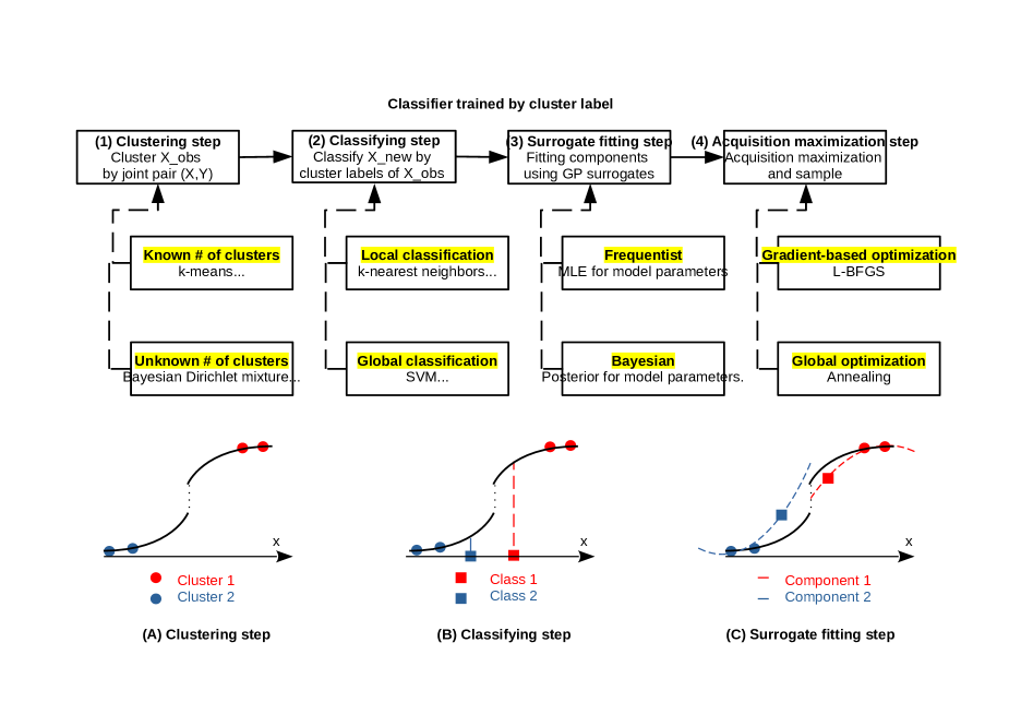
Figure 2.1: The cluster-classify algorithm for partitioning in the cGP surrogate model. In each step, we illustrate options for the task and highlight these options. In the bottom panel, we illustrate how the cluster-classify algorithm works for a one-dimensional non-smooth function according to the bullet list on page 1. In the illustration, we use solid lines to indicate black-box function $f$ and dashed lines for the fitted surrogate model $g$.
(A) There are 4 pairs of observations $(\bm{x},y)$, and the clustering algorithm clusters them into 2 clusters, represented by circles colored in red and blue.
(B) There are 2 new locations $\bm{x}_{1},\bm{x}_{2}$ represented by squares. The classification algorithm classifies these two locations into different clusters, represented by different colors.
(C) We use the corresponding surrogate component to predict at these 2 new locations $\bm{x}_{1},\bm{x}_{2}$. Using $(\bm{x}_{1},y_{1})$ and $(\bm{x}_{2},y_{2})$ we can update each component of the surrogate model.

1. (Clustering step) Cluster pairs $(\bm{x},y)$, with the clustering method you choose (e.g., if you do not know the number of clusters, Bayesian Dirichlet GP mixture (DGM) (Teh, 2010) works; if you know the number of clusters, $k$-means (Devroye et al., 2013) works). can attach cluster labels to samples $\bm{x}$ and form classes among samples . This step labels the observed locations and takes cluster labels as class labels for each location $\bm{x}$.

2. (Classifying step) Classify $\bm{x}_{new}$ by a classification method trained by the labeled samples $\bm{x}$ (e.g., $k$-nearest neighbors (k-NN, (Devroye et al., 2013)) provides a local classification; a support vector machine provides a global classification.) The new predictive locations $\bm{x}_{new}$ (without knowledge of corresponding responses) can be assigned to one and only one cluster class. In each sampling step, the clustering step (re-)labels the observations; and the classifying step is (re-)trained using the labels and predicts on domain.

3. (Surrogate fitting step) Construct additive GP modeling over the partition and fit it by either a frequentist or Bayesian approach.

4. (Acquisition maximization step) Maximize the modified acquisition function (See details in Appendices A and E) for each component (e.g., expected improvement, which concerns maxima of the black-box function) using a selected (gradient-based or global) optimization algorithm to determine the next sequential sample.

To familiarize the novel notion of cluster-classify step, we use $k$-means and DGM (introduced below) in the cluster step of all examples; but use only k-NN in the classify step of all examples in the current paper. However, our implementation supports a wide variety of clustering and classification algorithms used in machine learning. In the cluster-classify scheme, the k-means use the proximity of pair $(x,\xi y)$ to cluster sampled observations; and the k-NN use only the proximity of $x$ to classify any location $x$ without the knowledge of $y$.

Following the Gaussian process modeling notation (Rasmussen and Williams, 2006), the overall clustered GP surrogate model (with $k$ clusters) for a sample
$\left\{y_{1}(\bm{x}_{1}),\cdots,y_{n}(\bm{x}_{n})\right\}$ at $n$ different locations $\bm{X}=\{\bm{x}_{1},\cdots,\bm{x}_{n}\}$ takes the following vector form:

$$\bm{y}(\bm{X}) =(y_{1}(\bm{x}_{1}),\cdots,y_{n}(\bm{x}_{n}))^{T}=\sum_{j=1}^{k}\bm{f}_{j}(\bm{X})\cdot\bm{1}_{j}(\bm{X})+\bm{\epsilon},$$ (4)

where the $\bm{f}_{j}(\bm{x})=(f_{j}(\bm{x}_{1}),\cdots,f_{j}(\bm{x}_{n}))^{T}$ denotes the vector of the $j$-th scalar function evaluated at $n$ different locations $\bm{X}=\{\bm{x}_{1},\cdots,\bm{x}_{n}\}$ of all $k$ Gaussian mean components; the overall Gaussian noise $\bm{\epsilon}$ has mean $0$ and variance $\sigma_{\epsilon}^{2}$. $\bm{1}_{j}(\bm{x})$ is an indicator function returning 1 if $\bm{x}$ is classified as belonging to the $j$-th class and 0 otherwise.

In contrast to a hierarchical partitioning model like the sparse additive Gaussian process (SAGP) model proposed by Luo et al. (2020b); Park and Choi (2010), the additive components of this model are mutually independent due to the disjoint partition scheme induced by our cluster-classify procedure. In the cGP model (4), each $\bm{f}_{j}$ is modeled by a zero-mean Gaussian process prior, i.e., $\bm{f}_{j}(\bm{x})\sim N_{n}(\bm{0},\bm{K}_{j})$, where the notation $N_{d}(\bm{m},\Sigma)$ denotes the $d$-dimensional Gaussian distribution with mean vector $\bm{m}$ and covariance matrix $\Sigma$, with covariance matrix $\bm{K}_{j}=\left[K_{\bm{\kappa}}(\bm{x}_{r},\bm{x}_{s})\cdot\bm{1}_{j}(\bm{x}_{r})\cdot\bm{1}_{j}(\bm{x}_{s})\right]_{r,s=1}^{n}$ and the covariance kernel $K_{\bm{\kappa}}$ modeling the dependence between $\bm{x}$ within the same $j$-th class.

To evaluate the acquisition functions and determine the next sequential sample, we need to fit the surrogate model and draw predictions from the surrogate model. The model parameters are the kernel parameter $\bm{\kappa}$ that determines $K$ and the error variance $\sigma_{\epsilon}^{2}$. One approach to fit the model is to estimate the parameters by maximizing the likelihood function $L(\bm{\kappa},\bm{\sigma}_{\epsilon}^{2}\mid\bm{1}_{1}(\cdot),\cdots,\bm{1}_{k}(\cdot),\bm{y},\bm{x}_{1},\ldots,\bm{x}_{n})$ of (4), which is usually known as the “frequentist approach”. Alternatively, we can impose priors on the parameters $\bm{\kappa},\bm{\sigma}_{\epsilon}^{2}$ and use the modes of their joint posterior

$$P(\bm{\kappa},\bm{\sigma}_{\epsilon}^{2}\mid\bm{1}_{1}(\cdot),\cdots,\bm{1}_{k}(\cdot),\bm{y},\bm{x}_{1},\ldots,\bm{x}_{n})\propto$$

$$\underbrace{P(\bm{y}\mid\bm{\kappa},\bm{\sigma}_{\epsilon}^{2},\bm{f}_{1},\cdots,\bm{f}_{k})\prod_{j=1}^{k}P(\bm{f}_{j}\mid\bm{1}_{j}(\cdot),\bm{x}_{1},\ldots,\bm{x}_{n})}_{\text{Likelihood Function}}\cdot$$

$$\underbrace{P(\bm{\kappa}\mid\bm{1}_{1}(\cdot),\cdots,\bm{1}_{k}(\cdot))}_{\text{Kernel Prior}}\cdot\underbrace{P(\bm{\sigma}_{\epsilon}^{2})}_{\text{Error Prior}}.$$

as their estimates. This is usually known as the “(fully) Bayesian approach”.

The Bayesian approach is preferred by multiple authors (Snoek et al., 2012, 2014; Gramacy, 2020) for its flexibility of incorporating prior information and reproducibility. However, the frequentist approach is still widely used due to its computational efficiency and clear convergence criteria.

Our main idea follows the scheme on page 2.3 and Figure 2.2. We create labels for locations in the input domain based on $(d+1)$-dimensional pairs $(\bm{x}_{obs},y_{obs})$ by clustering (unsupervised). Then, we compute the decision boundary of a classifier trained by $\bm{x}_{obs}$ and its cluster labels, to induce a partitioning of the input domain. We expect that sample points that belong to different regimes determined by the non-smoothness would be assigned to different partition components.

With this trained classifier (supervised), we can classify any point $\bm{x}_{new}$ in the $H^{d}$ and form a partition over the domain. Then the (weighted) acquisition function (by default we use the expected improvement (EI) as the acquisition function) based on the surrogate model is maximized over each component. This weighted acquisition function can be applied to different kinds of acquisition functions like UCB or PI (Hernández-Lobato et al., 2014), we provide a theoretic justification of this weighting scheme in the additive surrogate model in Appendix E. In short, such a weighting scheme and the exploration rate below would ensure convergence of the Bayesian optimization procedure based on cGP.

In a broader view, this cluster-classify scheme also introduces a model selection problem in an online context. When the data accumulates, we want to determine the number of clusters dynamically. Currently, we retrain the clustering algorithm in every step, but to reduce the computational complexity, a more principled way might be to derive an online version of selection criteria like the gap statistics developed by Tibshirani et al. (2001).

We have to point out again that we consider noisy observations, and we pick the expected improvement (Shahriari et al., 2016) as our default acquisition function. However, if a noiseless model is assumed, a different choice of acquisition function is needed. Our algorithm is described in Algorithm 1, and we call this model the clustered Gaussian process (cGP) model.

The cGP model is intrinsically related to at least two different kinds of (Bayesian) GP models. One is the treed GP model (Gramacy and Lee, 2008) that partitions the input domain using a dynamic tree (hence not clear how acquisition function can be elicited for an online setting), while the cGP uses a more flexible way of component creation via the cluster-classify step. The other is a (two-layer) hierarchical model with input clusters (Park and Choi, 2010), but the hierarchical model requires latent parameters and user-specific clusters, and it is unclear whether the existing acquisition functions are still suitable if used in an online setting, compared to the cGP model as a simple additive model without latent parameters.

In the implementation of the cGP model, we introduce the notion of exploration rate, following the practice described by Bull (2011) (in Definition 4) in the spirit of reinforcement learning (Sutton and Barto, 2018). The exploration rate is the probability that the next sequential example would be sampled according to the acquisition maximization. When the exploration rate is exactly 0, the sequential samples are all randomly chosen without referring to the acquisition function at all. When the exploration rate is exactly $1$, the sequential samples are all sampled according to the maximizer of the acquisition function. In our specification, we default the exploration rate to be 0.8. It is worth pointing out that adjusting the exploration rate would affect the efficiency with which the sequential sampling explores the domain. In the algorithm described in Appendix A, we can see how this exploration rate controls alternating between acquisition maximization and random sampling schemes. We introduce this element to allow different sequential sampling schemes and investigate its effect in Section 3.1.

Another minor adjustment we introduce in our implementation is to add a boundary penalty function to the acquisition function. In the problem of handling non-smoothness, it seems that it is of benefit to sample more near the boundary of the partition. In an offline context, Park et al. (2011) had discussed thoroughly about the effect of partition boundaries in GP modeling. In the online optimization context, we implement a user-specified additive penalty function (normalized to the same scale) adding to the acquisition function, therefore, the maximization step would be biased towards the boundary of a component. For instance, the penalty function of a specific component can be configured to be proportional to the squared distance of a point to the boundary of this component. As the partition components determined by the cGP algorithm updates according to sequential sampling, this penalty function can also be updated to account for updated partitions as well. We recommend a careful penalty adjusted to the design and constraints on the domain or no penalty by default.

Figure 2.2: The algorithm flowchart for the cGP surrogate model. The dashed line indicates the usual GP surrogate model, which does not include a partition scheme. The detailed psuedo-code is available in Appendix A. Note that in each step, the clustering and the classifiers are re-trained with the newly sampled observation. Detailed pseudo-code for this algorithm is in Algorithm A.

Our cGP model can address the challenges in Section 2.2 while not introducing too much complexity in surrogate modeling:

• Limited and sequential samples. We do not introduce more complex parameterizations for the partitioning scheme induced by clustering, except for the parameters required by the additive GP components. Even with few samples, unlike more parameterized and complex models (Damianou and Lawrence, 2013; Herlands et al., 2016), cGP models can still be fitted in an online context.

• High-dimensional generalizations. We do not have a high computational cost even in a high-dimensional domain, since the clustering and classification algorithm are usually not affected by the curse of dimensionality. The major computational cost is fitting the component GP surrogate model.

• Restrictive partition shape. We introduce the cluster-classify procedure to determine the partition scheme. Since the classification boundary determines the partitions, we expect that the shape of partitions would reflect non-smoothness better.

We also point out that cGP is unable to model non-smoothness within a single component by its construction. In an extreme situation, we pick only two points, $x_{1}=-0.5$ and $x_{2}=0.5$ for $f_{1}$ function with $f_{1}(x_{1})=1.5,f_{1}(x_{2})=0.25$ as shown in Figure 1.1. If we treat $x_{1},x_{2}$ as one cluster, then we fail to capture the non-smooth point $x_{*}=0$ and will have a constant mean function at $0.375$. If we treat $x_{1},x_{2}$ as two clusters, then we will have piecewise constant functions of values $0.5$ and $0.25$ respectively with a non-smooth change-point at $0$. This problem is intrinsic to any partition-based method with a mis-specified partition scheme. Empirically, we observe that this is not a too serious issue for cGP if we have enough pilot samples.

3 Experiments

Subsection 3.1 starts with simple illustrations of our proposed cGP model. Then, subsection 3.2 revisits the motivating tuning problem we briefly mentioned in Section 1.1 and qualitatively compares the performance of different surrogate models. We first showed that cGP is a competitive alternative for simple smooth and non-smooth functions. Then in matmul, piston and SuperLU applications, our cGP model shows considerable improvement in tuning results. In specific synthetic functions (i.e., Bukin.N6), the improvement is strict in 90% of repeated experiments. The partitioned regime identified by the cGP model is also described and discussed.

3.1 Synthetic Studies

To establish an intuition of how the cGP surrogate model and Algorithm 1 behave, we show two synthetic examples in $H^{2}\subset\mathbb{R}^{2}$. These low-dimensional examples allow us to examine the results visually and qualitatively along with quantitative summaries.

3.1.1 Smooth functions

First, we want to consider a smooth black-box function and see if cGP is competitive against GP surrogates when there is no non-smoothness. In this situation, we expect a simple GP surrogate to perform the best, but expect that cGP models are also competative. Since when we choose the number of clusters $k=1$, the cGP model reduces to the usual GP model, we also expect that GP and cGP would have similar fits when $k$ is small. In the situation where the black-box function has no non-smoothness, for example, we take the simple function $f_{3}(\bm{x})=f_{3}(x_{1},x_{2})=1/(1+(x_{1}-0.25)^{2}+(x_{2}-0.25)^{2})$. We examine one sample of cGP fits (with Matérn $3/2$ kernels) for $k=1,2,\cdots,5$ in Figure 3.1 and average performance in Table 3.1.

When we try to maximize the function, the two key statistics we observe are

$$\Delta\arg\max\coloneqq\|\arg\max_{\bm{x}}(f)-\text{sample maximum point }\bm{x}\|_{2}$$

the $L_{2}$ distance between sample maximum point $\bm{x}$ and the exact maximum point, and the

$$\Delta\max\coloneqq|f_{\max}-\text{sample maximal observed }y|$$

which is the difference between sample maximum function value $y$ and the exact maximum value $f_{\max}=f(\arg\max_{\bm{x}}f)$.

In the optimization context, smaller statistics $\Delta\arg\max$ indicate better performance of the surrogate model, which leads to a sample maximum closer to the truth. And smaller statistics $\Delta\max$ indicates the surrogate model finds an (possibly noisy) observed value that is closer to the true function value.

We can see that for this $f_{3}$ with the unique maximum 1 attained at $(1/4,1/4)$, only the case $k=3$ gives significantly worse performance than the simple GP models in one fit in Figure 3.1, but reasonably close to simple GP on average. And we can see that cGP performs very closely to the simple GP surrogate as shown in Table 3.1; as the number of $k$ increases, the surrogate fits improve.

Surrogate	$f_{3}$ (smooth, Figure 3.1)		$f_{4}$ (non-smooth, Figure 3.2)
	$\Delta\arg\max$	$\Delta\max$	$\Delta\arg\max$	$\Delta\max$
GP ($k=1$)	0.018718	0.000349	0.082762	0.006721
cGP ($k=2$, $k$-means)	0.034503	0.001182	0.067821	0.004524
cGP ($k=3$, $k$-means)	0.041824	0.001730	0.085938	0.007180
cGP ($k=4$, $k$-means)	0.028472	0.000808	0.078971	0.006084
cGP ($k=5$, $k$-means)	0.026969	0.000724	/	/
cGP ($k=2$, DGM)	/	/	0.082752	0.006623
cGP ($k=3$, DGM)	/	/	0.078508	0.006031
cGP ($k=4$, DGM)	/	/	0.067031	0.004412
cGP (partitioned)	/	/	0.160008	0.022961

Table 3.1: Average statistics $\Delta\arg\max$ and $\Delta\max$ for the repeated 50 experiments (different random pilot samples) for synthetic functions $f_{3}$ and $f_{4}$. The smallest statistics (indicating the best model in terms of this statistics) in each column are shown in bold fonts.

This set of synthetic experimental results supports that the cGP method performs reasonably when the black-box function is smooth and would not create a lot of non-smoothness in the fitted surrogate model. Averaging over multiple runs with different pilot samples leads to similar results, therefore, we conclude that adopting the cGP model would not create comparable tuning results on average compared to GP surrogates even there is no non-smoothness at all.

3.1.2 Non-smooth functions

Second, we want to see how cGP performs when non-smoothness exists in the black-box function, compared to GP. We create some non-smoothness in the function $f_{3}$ along the line $x_{2}=0$. We use the indicator function $\bm{1}(\cdot)$ to complete the construction. $f_{4}(\bm{x})=f_{4}(x_{1},x_{2})=\bm{1}(x_{2}>0)\cdot(1/(1+(x_{1}-0.25)^{2}+(x_{2}-0.25)^{2}))+\bm{1}(x_{2}\leq 0)\cdot(0.25/(1+(x_{1}^{2}+x_{2}^{2})))$ as shown below with the same unique exact maximum point (1/4,1/4) as $f_{3}$. Therefore, if the non-smoothness introduced by the indicator functions does not affect the surrogate-based optimization at all, then we would be able to locate the maximum value of $f_{4}$ as easily as $f_{3}$. We examine the mean of cGP fits (with Matérn $3/2$ kernels) for $k=1,2,\cdots,4$ in Figure 3.2 using both $k$-means and Dirichlet Gaussian mixture (DGM) as clustering algorithms. In this case, $k=1$ (i.e., simple GP surrogate) is underfitting and cGP with $k=3,4$ are overfitting since we know from its expression that there are exactly two continuous regimes of this function, separated by the straight line $x_{2}=0$, in the true black-box function $f_{4}$.

Since the cGP model consists of two main parts, the cluster-classify step to get the partitions and modeling on the partitions, we want to explore how the cGP model works when the exact partitioning is known, and compare to the results when the partitions must be computed. Following the practice in Figure 1.1, we get a partitioned cGP assuming that we know the partition is given by $x_{2}=0$. The panel “cGP (partitioned)” in Figure 3.2 shows that when we know the partition exactly, an additive GP (i.e., cGP with known partition) produces the best surrogate fit among all models when compared to the truth of $f_{4}$. In short, if we know the exact partition, then we should not use cluster-classify step, but the model with the exact partition components directly (i.e., additive GP) in this sequential sampling context. Our algorithm Algorithm 1 can be shown to converge when the exact partition is fixed, see Proposition 3 in Appendix E.

When $k=3$, the non-smoothness at $x_{2}=0$ cannot be modeled very appropriately with either $k$-means or DGM as we observe. The cGP with $k=1$ (i.e, GP) is over-smoothed, while the cGP with $k$-means ($k=4$) does not capture a transition boundary near $x_{2}=0$ well. The cGP with $k$-means($k=2$) and DGM ($k=3$) captures the $x_{2}=0$ better, with optima similar to the true black-box function. The cGP with DGMs all have smaller $\Delta\arg\max$ compared to GP and reasonable improvement, while cGP models with $k$-means ($k=2,4$) DGM ($k=2,3,4$) have better $\Delta\max$ and $\Delta\arg\max$ compared to a simple GP on average as observed from Table 3.1. This means that with the same limited sample budget, cGP models (with appropriate clustering) get closer to the true maximum value. We observe that a cGP model with DGM performs better in terms of identifying clusters. The number of clusters is selected by the DGM with a prespecified maximal number of clusters (Teh, 2010). DGM does not require us to know the number of clusters $k$ exactly but the algorithm learns this number from sequentially sampled data. As shown, we can see that DGM with the maximal number of components being 3 adjust the number of partitions better and performs better compared to $k$-means with $k=3$, as shown by one run in Figure 3.2.

One more observation we made based on the average statistics shown in Table 3.1 is that we can see that compared to $f_{3}$, $f_{4}$ tends to inflate the two statistics, no matter what surrogate model we use. This strengthens and is consistent with our intuition established in Figure 1.1 that when there exists non-smoothness, the Bayesian optimization based on surrogate models would encounter difficulties due to the lack of fit near the non-smooth points. In this non-smooth example, we only change the maximal number of clusters allowed in DGM (e.g., in Figure 3.2, we show the $k$ parameter and the number of clusters finally chosen as well).

black-box $f_{3}\in[8/33,1]$ GP ($k=1$) $k$-means ($k=2$) $k$-means ($k=3$) $k$-means ($k=4$) $k$-means ($k=5$)

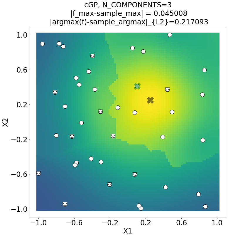
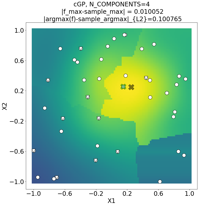
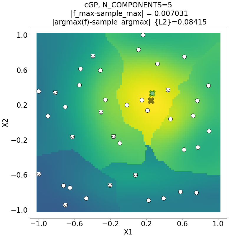
Figure 3.1: Mean function and partition scheme extracted from the GP surrogate model evaluated on $100\times 100$ equally spaced grids on $[-1,1]^{2}$ with weighted expected improvement acquisition function and $n=10$ random pilot samples (triangles), $n=30$ sequential samples (circles) from $f_{3}$. We use the same clustering methods with different assumed numbers of clusters: $k$-means (with $k=1,2,3,4,5$). We show exact minimal point by a black cross; sample minimal point by a green cross.

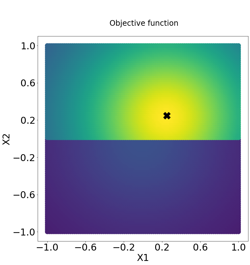
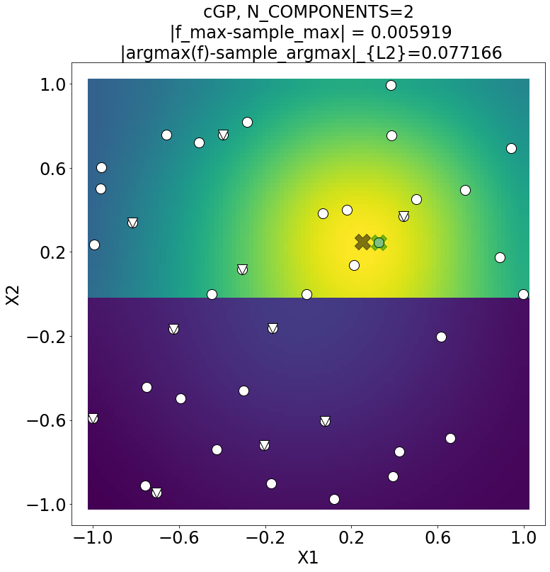
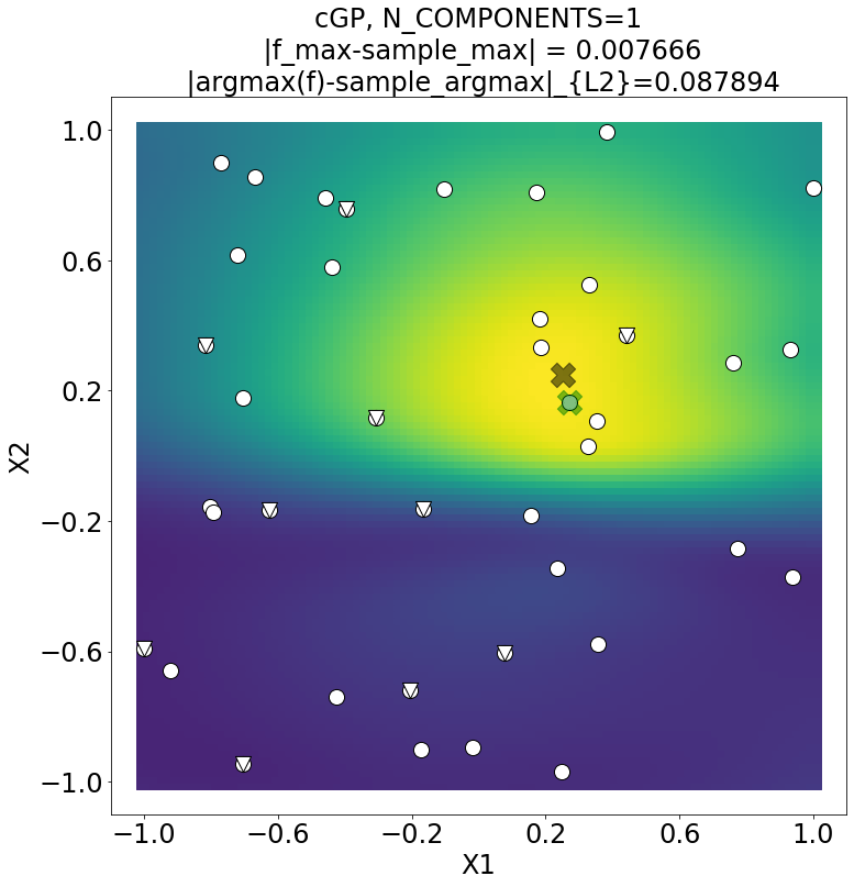
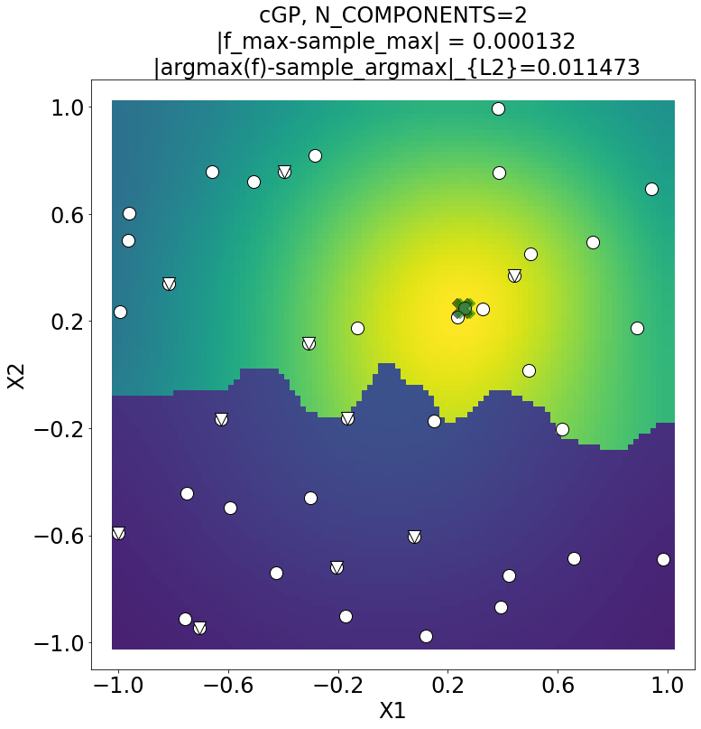
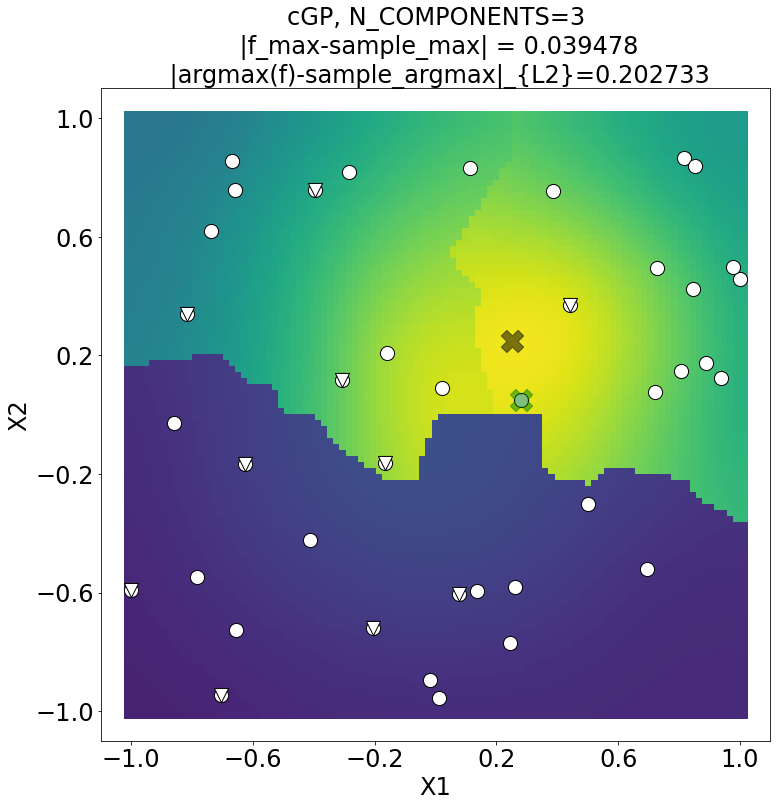
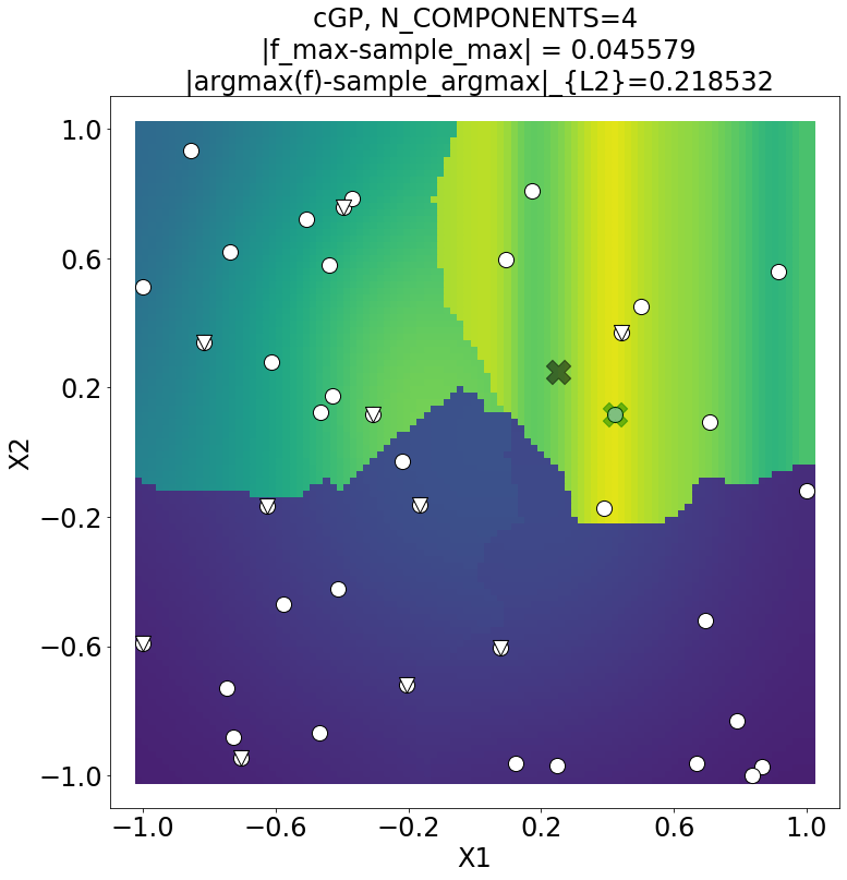
black-box $f_{4}\in[1/3,1]$ cGP (partitioned) GP ($k=1$) $k$-means ($k=2$) $k$-means ($k=3$) $k$-means ($k=4$) DGM ($k=2$, fits 2) DGM ($k=3$, fits 2) DGM ($k=4$, fits 4)

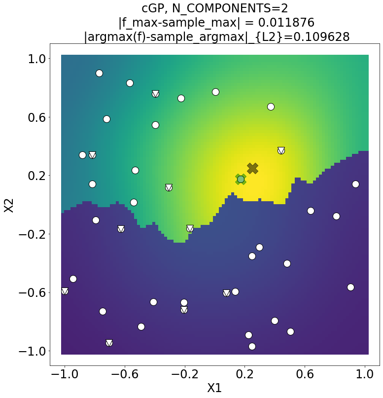
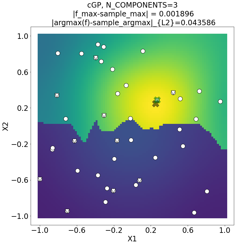
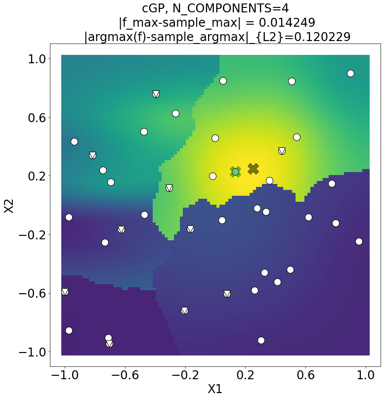
Figure 3.2: Mean function and partition scheme extracted from the GP surrogate model evaluated on $100\times 100$ equally spaced grids on $[-1,1]^{2}$ with weighted expected improvement acquisition function and $n=10$ random pilot samples (triangles), $n=30$ sequential samples (circles) from $f_{4}$, We provide the cGP with oracle partition ($x_{2}=0$) in cGP (partitioned) panel. We use different kinds of clustering methods: $k$-means (with $k=2,3,4$), Dirichlet Gaussian Mixture (DGM, the algorithm fits the surrogate with $2,3,4$ clusters when the maximal allowed number of components are 2,3,4, respectively.) We show exact minimal point by a black cross; sample minimal point by a green cross.

Furthermore, the choice of clustering algorithm in the cluster-classify step matters. When $k=2$ the fit of cGP with $k$-means clustering seems to capture the non-smoothness well while retaining the behavior that is similar to the underlying function. However, in practice, we do not know how many clusters are there. One approach is to treat $k$ as a hyper-parameter that is subject to further tuning with model selection criteria or cross-validation on real data. The other approach, which we take here, is to use Dirichlet Gaussian mixture. We show the fit of these latter two approaches in Figure 3.2 with $k=2,3,4$. Figure 3.2 serves as a qualitative verification of our method in a low-dimensional domain ($d=2$). Usually, a reasonably large $k$ (e.g., 3,4) and DGM would be a practical choice for cluster-classify step whenever our sampling budget allows.

The illustrative examples above show how cGP behaves in terms of mean function and error statistics. cGP behaves differently as we change the number $k$ of components and clustering algorithms. Note that since we use expected improvement (EI) as our guiding acquisition function throughout the paper, it is expected that the $\|f-g\|_{\max}$ would accumulate from clusters, hence possibly worse than the GP.

Next, we want to see how the sequential sample size $n$ and exploration rate $\tau$ could change the behavior of the cGP model when compared to the GP model. As a third example, we study a well-known benchmark function called Bukin N.6 function (displayed in Figure 3.3) defined on a 2-dimensional domain.

We experiment with cGP surrogates with exploration rates $1$ (always sample based on acquisition maximization), $0.8$ and $0.5$. When the exploration rate is 0, the sequential samples are all randomly chosen; while when the exploration rate is 1, the sequential sampling is fully based on acquisition maximization. In some situations (like matmul in Sec. 3.2), adjusting the exploration rate would allow us to explore the domain more efficiently.

For now, let us see how different exploration rates would affect the performance of cGP surrogate models. In this set of experiments, we first investigate the distribution of optima found by different surrogate models. In the first row of Figure 3.4, we repeat the optimization for 100 different random seeds and we can see that when there are moderate or sufficient sequential samples ($n=90,190$), cGP surrogates produce $f_{\min}$’s that are lower (hence better) than the optima given by the GP surrogate with the same sample size. When there are only limited samples ($n=10$), cGP seems to have small improvements. In each of the box plots, we can see that this comparison is systematic and not due to randomness. It is not hard to see in the second row of Figure 3.4 that, partition schemes are actually capturing the level sets of Bukin N.6 function rather accurately and sample more near the optima. Quantitatively, we provide the percentages that cGP surrogates (under different combination of exploration rates) outperform their GP counterparts among 100 runs with distinct random seeds. We not only provide the percentages that cGP gives equal or strictly smaller $f_{\min}$, but also the percentage that cGP gives strictly smaller $f_{\min}$. The percentage that cGP gives equal or strictly smaller $f_{\min}$ should be over 50% to justify the use of cGP, and a larger percentage of strictly better optima indicates the superiority of cGP.

This experiment shows a consistent and qualitative advantage of cGP over GP surrogates. However, more importantly, it also shows that different configurations of hyper-parameters in the cGP model can be adjusted to yield better performance over the same function. The partition scheme accompanying the cGP surrogate fit also reveals the nontrivial geometric structure of the black-box function. Empirically, we find cGP fits slightly faster compared to GP when $n=190$, since inverting $k$ smaller covariance matrices costs less than 1 large covariance matrix of GP. In general, if the black-box function has optima in a relatively small region compared to the whole domain or the function has non-smoothness (also sharp changes) near optima, then the cGP surrogate may reach better optima compared to the GP surrogate, and run faster. And cGP can identify different kinds of behavior rather faithfully through the cluster-classify procedure. Even if the cGP fails to capture the different behaviors in the domain, we still observe that cGP has competitive performance when compared to GP (which is consistent with Figures 3.1 and 3.2).

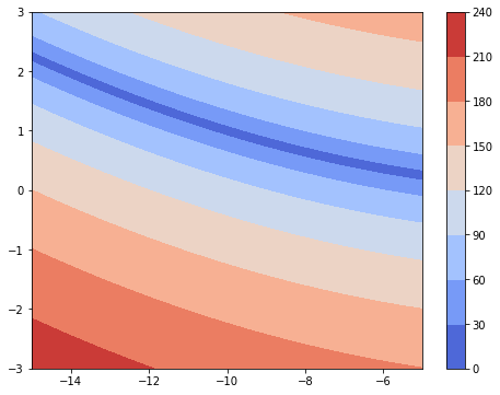
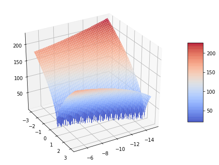
Figure 3.3: The Bukin N.6 function is defined by $f(x)=100\sqrt{|x_{2}-0.01x_{1}^{2}|}+0.01|x_{1}+10|$. The function has unique global minimum $f(x_{\ast})=0$ at $x_{\ast}=(-10,1)$. We optimize the function to find its minimum over the domain of $(-15,5)\times(-3,3)$. The plot is based on evaluation of $f(x)$ on a 100 by 100 grid.

$k=2$ $k=3$ $k=4$

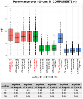
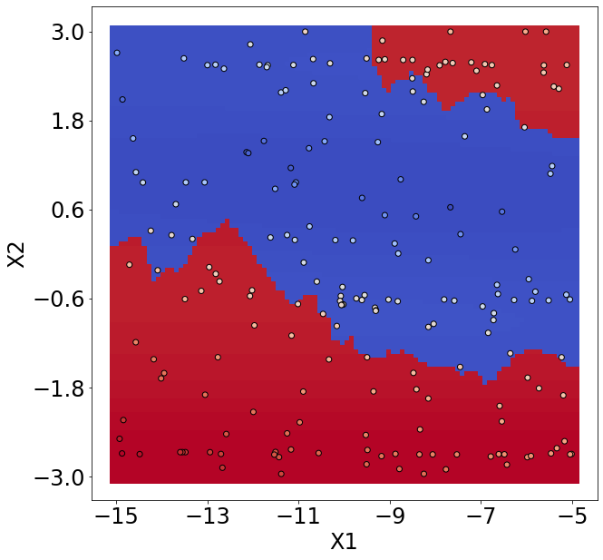
Figure 3.4: The box plot of optima (minimum) obtained from the cGP surrogate model with exploration rates (expRate) of 0.5, 0.8 and 1.0, 10 pilot samples and a sequential sample of size (seqSize) $n=10,90,190$ from Bukin N.6 function. Each dot on the box plot means one optimum obtained from one random seed. We display the performance in terms of distribution of optima from sequential samples from GP and cGP surrogate models, with different numbers of components, exploration rates and sequential sample sizes.
In the percentage table, “(equal)” columns show the percentage of cGP fitted surrogates with optima equal or better than the baseline GP surrogate under different exploration rates in 100 different random seeds. “(strict)” columns shows the percentage of cGP fitted surrogates with optima strictly better than the baseline GP surrogate under different exploration rates in 100 different random seeds.
We also provide corresponding partition schemes (different clustering components are indicated by different colors) for one fit of cGP surrogate model with 190 sequential samples.

3.1.3 Summary

We explore the effect of hyper-parameters of the cGP surrogate model in this section. With qualitative distributional summaries of experiments like box plot and quantitative analysis introduced, we present evidence that cGP has advantages over classical GP surrogates:

1. In the smooth function example (Figure 3.1), we observe that cGP with small $k$ performs similarly to GP. When there is no non-smoothness in the black-box function, we can use cGP in place of GP without much loss of performance. In fact, GP is a special case of cGP with $k=1$.

2. In the non-smooth function example (Figure 3.2), we observe that cGP with different $k$’s can outperform GP when $k$ is appropriately chosen. When there is non-smoothness in the black-box function, we can use cGP to improve optimization results and adjust hyper-parameters. cGP would also produce a partition scheme that illustrates the non-smooth behavior in the black-box function.

3. In the Bukin N.6 function example (Figure 3.3), we observe that cGP with different exploration rates and sample sizes outperforms GP under the same conditions, but different configurations of these hyper-parameters can affect the optimization performance of cGP. In this example, cGP produces a partition scheme illustrating a non-trivial structure of the black-box function and yields better optima.

cGP has the potential of detecting the non-smoothness in the black-box function and cGP usually performs at least as well as GP. We include further synthetic study evidence in Appendix B to support this claim. In the next section, we investigate the performance of the cGP surrogate model in real tuning problems.

3.2 Tuning Problems

As we explained in our cGP model specification above, there are quite a few (hyper-)parameters we could select for the cGP surrogate model.

In a general application, the default choice would suffice. We run some pilot experiments and choose the model parameters like the maximal number of components and exploration rate sequentially. Although the most rigorous way is to find a grid of all possible combinations of these parameters and conduct an exhaustive search, empirical choices would also help. For example, we could guess how many components are there in the black-box functions from the observed data.

The first example is a classic low-dimensional tuning problem, that is to find an appropriate blocking to improve the performance of a large matrix multiplication. We focus on the challenge of limited sample sizes. The second and the third examples, on the other hand, have rather high-dimensional parameter spaces, and hence the difficulty to fit a surrogate model in a high-dimensional parameter space will be present. One of them uses the piston cycling function, the other involves the tuning of the sparse matrix factorization time in the SuperLU_DIST package (Yamazaki and Li, 2012).

3.2.1 Low-dimensional tuning

Let us revisit the matrix multiplication tuning problem we mentioned in subsection 1.1. The black-box function is the computational speed function of the operation $A*B=C$ with blocking structure, where the $n\times n$ matrices $A,B,C$ have double precision entries, and consist of $N\times N$ blocks each of size $b\times b$ such that $n=Nb$. The parameter we attempt to tune is the shared block size $b$ and the computational speed function $f(b)$. Therefore, we have six nested loops (3 outer loops to perform $N^{3}$ multiplications of $b\times b$ matrices, and 3 inner loops to perform 1 $b\times b$ matrix multiplication). Let $m$ be the amount of memory traffic (i.e., slow communication) between main memory and cache, and $f$ be the number of floating point operations. In this example, we have the following analytical performance model:

$$m= N\cdot n^{2}+N\cdot n^{2}+2n^{2} \text{ read each block of }A,B\text{ }N^{3}\text{ times},N^{3}\cdot b^{2}=N\cdot n^{2}$$

$$= (2N+2)n^{2} \text{ read and write each block of }C\text{ }1\text{ time},2N^{2}\cdot b^{2}=2n^{2}$$

$$f= n^{3}+n^{3} \text{number of additions,}N^{3}\cdot b^{3}=n^{3}$$

$$= 2n^{3} N^{3}\cdot b^{3} n^{3}$$ and number of multiplications, =

The quotient $q=f/m$ of these two quantities, known as computational intensity, can be used to model the computational speed of the matrix multiplication. It can be calculated as $q=f/m=\frac{2n^{3}}{(2N+2)n^{2}}\approx b\text{ as }n\rightarrow\infty,\text{s.t. }n=Nb$. Therefore, based on this analytical performance model, we can optimize (maximize) the function $q(b)$ by increasing the block size $b$ (denoted as $\bm{x}$ below). However, this analytical model has an implicit assumption: the 3 $b\times b$ blocks always fit into the cache. We want to increase the block size to reduce communication but also avoid overflowing the cache, which would cause a sudden decrease in performance. Hong and Kung (1981) proved that the minimum number of words moved between cache of size $M$ and memory is $\Omega(\frac{n^{3}}{\sqrt{M}})$ which corresponds to $q\approx b=O(\sqrt{M})$. The exact optimal value of $b$ depends on details of how the loops are organized, compiler optimizations, and hardware architecture, which has led to a large literature on the topic, including the development of special purpose autotuners. More details of optimization for matrix multiplication are explained by Bilmes et al. (1997), Whaley et al. (2001) and Zee et al. (2016). Our goal is not to compete with these autotuners, which may include custom code generation as well as tuning parameters, but to use matrix multiplication as a motivating example, where clear non-smooth and different regimes can be observed, for the clustered GP surrogate.

Figure 3.5: The computational speed for matrices of size $n=1000$. This is the true black-block function obtained from a Haswell node. We also use a green dashed line to indicate the actual maximum $(\bm{x}_{\text{max}},f_{\max})=(112,2010.702)$; and red dashed lines for the regime cutoff $\bm{x}=b=160,500$ discussed in the text.

The machine on which we conduct this experiment is a Cori Haswell computing node, with an L1 cache size of 32KB, 256KB for L2 cache and 40960KB for L3 cache. All cache-line sizes are 64 bytes, i.e., 8 double precision words. Each node has an Intel Xeon Processor E5-2698 v3 2.3 GHz processor (with a theoretical peak of 2.81 PFlops) with a 128GB memory.

Large matrix multiplication is quite expensive, and if we evaluate the computational speed of each block size $b$ from 1 to $n=1000$ (when the block size is 1 or 1000, there is no blocking). The L3 cache is large enough to fit all 3 $1000\times 1000$ matrices $A$, $B$ and $C$. Based on multiple runs, we observe that there is little noise in the data and do not consider averaging it further here. In this dataset, we can make preliminary observations that there are several different kinds of behavior, apart from the noise:

• When $b<160$, the speed increases rapidly with some oscillations and then drops to a plateau level. The oscillations, with local peaks at $b$ equal to multiples of 8, are to be expected since the cache-line size is 8 words. In practice, one might limit the search space to $b$ being multiples of 8, resulting in a smaller search space and a smoother function to optimize, but here we consider all values of $b$ to more rigorously evaluate the cGP. The optimal configuration is attained at $(\bm{x}_{\text{max}},f_{\max})=(112,2010.702)$, with the 2 second best configurations at $(120,2001.35)$ and $(128,2000.758)$. The choice of $b$ that minimizes memory traffic and so (potentially) maximizes speed, depends on details like the ordering of the loops, and what the cache chooses to keep inside or not. In particular, anywhere from just over 1 $b\times b$ to 3 $b\times b$ blocks may need to fit in cache. In our case, since $A$, $B$ and $C$ all fit in L3 cache, the question is what $b$ minimizes the traffic between L2 and L3. Since the L2 holds 32K words, this means it can hold at most 1 square block of size $b=181$, 2 of size $b=128$, and 3 of size $b=104$, ignoring cache conflicts, etc. So it is no surprise that the performance falls off rapidly past $b=128$, reaching a plateau around $b=160$. For a regular sampling scheme, it requires some more sampling in this interval to attain this point, as seen from Figure 3.6 (a) and (d), while cGP benefits from a good partitioning.

• When $160\leq b\leq 500$, the computational speed has a stable trend and rough behavior, with some fluctuations caused by memory alignment and code implementation. Again, most of the small peaks occur at multiples of 8.

• When $b\geq 500$, there is another significant drop (the trend can also be identified starting from $b=400$) until a roughly constant computational speed is attained.

We choose only 20 to 100 samples (including 10 pilot samples) when fitting surrogates so that our surrogate model with sequential sampling can be completed within 20 minutes (versus 3-4 hours needed for an exhaustive search) on the same machine configuration. However, to reduce randomness, we use the recorded dataset as the black-box function $f$ defined on $[1,1000]\cap\mathbb{Z}$. In Figure 3.6, we show the cGP with Dirichlet Bayesian Mixture clustering with maximal number of components as $3$ (which is also the actual number of components chosen), a $k$-nearest neighbor classifier ($k=3$), and a Matérn 3/2 covariance kernel (with nugget). We start with the same 10 randomly chosen pilot samples and then cap the total sample size at 20 and 100, respectively.

(a) GP, 10 sequential samples.	(b) GP, 90 sequential samples.
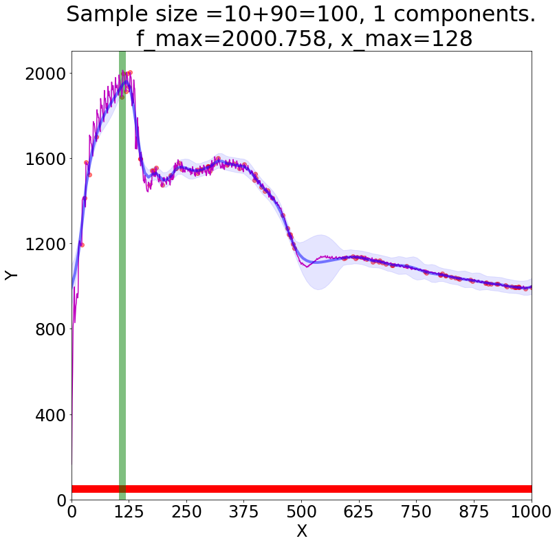
(c) cGP, 10 sequential samples.	(d) cGP, 90 sequential samples.

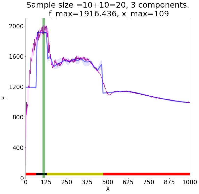
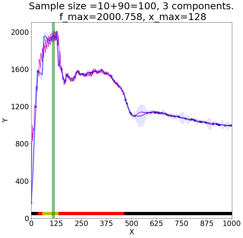
Figure 3.6: The computational speed function and fitted surrogate models. The dark blue solid line and light blue shaded area are the mean and variance of fitted prediction models. $(\bm{x}_{\text{max}},f_{\max})$ records the optimal block size and the actual optimal speed is illustrated by green vertical line on the figure. Bottom colored bars with different colors indicate to which cluster certain portions of the domain belong (but color has no semantic meaning). We also use magenta solid lines to overlay the truth from Figure 3.5 for comparison purposes. (The exploration rates of these experiments are all 1.)

We can get a first impression of the difference between GP and cGP surrogates by looking at Figure 3.6. When the sample size is 20, we can see that there is a big difference between the surrogate fits of GP and cGP, although their sample maxima are close. This difference is due to the fact that the clustering algorithm we choose gives us a correct cluster-based partition when there are as few samples as 20. When the sample size is 100, we observe that the cGP identifies the drop starting from $b=160$ and $b=500$ and attains maxima as good as $b=128$ (with $f(128)=2000.758$, close to the optimal $f(112)=2010.702$), and the same as GP. While its performance is similar to GP with larger sample sizes, we can see that cGP correctly identifies the change of function behavior caused by the drop of computational speed near $b=160$ and another behavior that changes rapidly when $b\geq 500$ even with very limited samples. Within each partition regime, the cGP provides a better fit in the sense that its mean function captures the sharp slopes caused by cache size. The main point we try to make here is that cGP can provide additional partition information while still maintaining a similar performance as GP in searching for maximum. This observation is further strengthened by the summary of repeated experiments in Figure 3.8.

(a) (b) (c) Exploration rate = 1.0 Exploration rate = 0.8 Exploration rate = 0.5

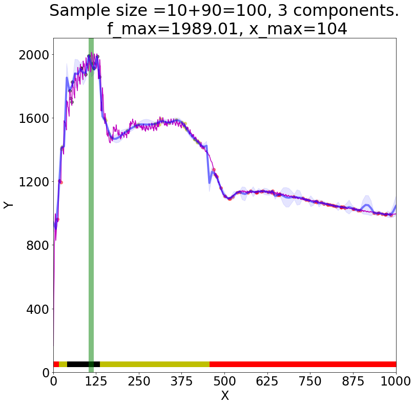
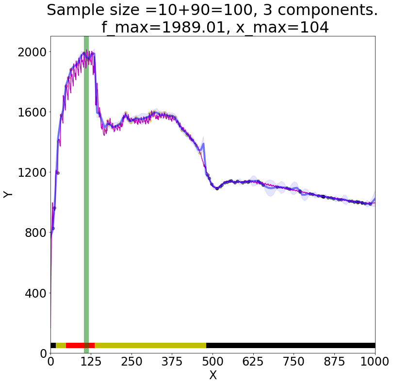
Figure 3.7: The computational speed function and fitted surrogate models. Bottom colored bars with different colors indicate to which component a certain portion of the domain belongs (but color has no semantic meaning). We also use magenta solid lines to overlay the truth from Figure 3.5for comparison purposes. The fit from GP surrogate model with 60 sequential samples and exploration rate (a) $1$. (b) $0.8$. (c) $0.5$.

So far, we consider all sequential samples selected by acquisition maximization (exploration rate 1). In Figure 3.7, we show how the cGP fit changes with different exploration rates, which are defined in the flowchart (see Figure 2.2) and affects the random sampling procedure. If the exploration rate is 0.6, then with a probability 0.6 we choose the next sequential sample with acquisition maximization; and with probability 0.4, we randomly choose the next sample from the input domain (i.e., a random block size $b$).

It is not difficult to observe from Figure 3.7 that, with a lower exploration rate, the partition components remain similar, where for all exploration rates the drops at $b=160$ and $b=500$ are clearly indicated by the change of additive components. However, with a lower exploration rate, we also observe that the sample locations are more spread over the input domain.

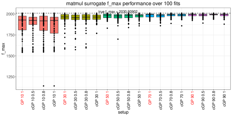
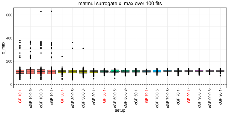
Figure 3.8: The box plot of $f_{\max}$ (top) and $\bm{x}_{\max}$ (bottom, log scale) elicited from sequential samples of 100 fitted surrogate models, each dot in the box plot represents the optimal point in each run (hence each box plot contains 100 points). The sequential sample size varies from 10 to 190 with 10 pilot samples. The exploration rates of the cGP model are chosen to be 0.5, 0.8 and 1 (x-axis format: model/sequential sample size/exploration rate).
Results for simple GP surrogates are highlighted with red labels as a baseline surrogate model; while cGP surrogates with different exploration rates are highlighted with black labels.

In Table 3.2, we also provide the percentage (among 100 runs with different shared random seeds) of runs that cGP outperforms simple GP surrogate models, as a quantitative supplement to the illustration in Figure 3.8, which supports the claim that our cGP surrogate models with the setups above (and different exploration rates) would consistently behave similarly like a simple GP surrogate model, while providing the non-smooth information of the black-box function in terms of both partitions and number of components. As the sequential sample size increases from 10 to 90 (see Table 3.2 (a)), we can see that both surrogate models behave similarly in terms of reaching optima, but the cGP model reaches the true optimum $b=112$ of the underlying black-box function more often (see Table 3.2 (b)). A medium exploration rate of 0.8 in the cGP model seems to improve the performance in this specific data application. Eventually, the number of additive components in the fitted cGP model stabilizes at around 2.9 (see Table 3.2 (c)), which is consistent with our observation that there are 3 partition regimes for the full recorded dataset. The average number of components is not exactly 3 since the $[1,80]\cap\mathbb{Z}$ partition component of the domain is usually under-sampled in surrogates with small sequential sample sizes.

In this matrix multiplication tuning example, the cause of non-smooth points (i.e., reduction of communication; overflow of fast cache) and different kinds of behavior is clear and observed in the recorded dataset as shown in Figure 3.5. cGP surrogates behave similarly to the GP model when there are few samples; but when there are enough samples, the cGP model clearly identifies different partition regimes much better with a reasonable performance in optimization. It is also clear that each additive component has a different normalization for the data within this label, hence different degrees of smoothness are better elicited in the surrogate fit. The non-smooth change-points between components are also captured in the cGP model. Therefore, the cGP model searches the optimum $f_{\max}$ and $\bm{x}_{\max}$ more efficiently compared to a simple GP surrogate. In short, cGP provides non-smooth information about the black-box function without loss of optimization performance compared to GP in this application.

In a different setting of matmul application, where we do not change our blocking strategy but vary the matrix size, we even witness the accuracy improvement by adopting the cGP as our surrogate model, see Appendix C.

(a) (b) (c) Exp. rate 1.0 0.8 0.5 1.0 0.8 0.5 GP 1.0 0.8 0.5 Sample size $n=10$ 0.72 0.66 0.62 2 2 1 2 2.71 2.64 2.63 $n=30$ 0.57 0.54 0.48 2 5 3 4 2.89 2.83 2.85 $n=50$ 0.55 0.51 0.45 4 8 6 9 2.84 2.91 2.86 $n=70$ 0.55 0.57 0.49 14 14 11 11 2.88 2.90 2.91 $n=90$ 0.54 0.63 0.54 15 19 16 13 2.94 2.94 2.97

Table 3.2: (a) The percentage of cGP fitted surrogates with optima equal or better than the baseline GP surrogate under different exploration rates. (b) The number of cGP (and GP) fitted surrogates that attain the actual optimal matrix size $\bm{x}_{\max}=112$ under different exploration rates in 100 different random seeds. (c) The average number of additive components in the fitted cGP surrogate models among 100 different random seeds.

3.2.2 High-dimensional tuning

We acknowledge that there are different definitions for high dimensionality. In the tuning context, we usually consider 3- to 32- dimensional domains as high-dimensional tuning domains. This is partially due to the fact that grid searches are no longer an effective strategy in these dimensions. When we conduct a grid search on a one or two dimensional domain, the grid size (i.e., the number of grid points) is usually of the magnitude of $10^{3}$ to $10^{6}$ when we use $\leavevmode\nobreak\ 1000$ grids in each dimension. However, when the dimensionality is 3, the magnitude grows to $10^{9}$, which takes a long time to enumerate. And when the dimensionality exceeds 32, even a binary enumeration vector would take more than $2^{32}$ bytes$=$32Gb to assign. This already exceeds the usual cache size of current computational machines, and makes the grid search infeasible.

In high-dimensional domains, the tuning problem can benefit from adopting surrogate models (Gramacy, 2020). Like the GP surrogate generalizes into high dimensions, it is possible to generalize our cGP model into a domain with higher dimensions. However, the limited sample size would restrict our focus since we need more samples to fit a higher dimensional surrogate model. In the existing literature, synthetic and real examples with dimensionality higher than 32 are seldom studied, with an exception by Chen et al. (2012).

3.2.2.1 Emulated piston cycle time ($d=7$). The first high-dimensional application we study is the piston cycle time model which was proposed in Kenett et al. (2013) for quality control in industrial applications, and has been well-studied in Owen et al. (2014). It is important to tune the variables (e.g., piston surface area, initial gas volume, etc.) of a piston to manufacture products whose minimum and maximum cycle time are within a certain range. This piston model function is a continuous function describing the cycle time of a piston, defined on a 7-dimensional domain with all of its tuning variables being continuous. Although the model function is continuous, empirically it does produce dramatic changes that make it almost look “non-smooth”, as we already observed in the Bukin N.6 function (Figure 3.3). In this specific application, both maximum and minimum are of interest. Therefore, we expect that we need to fit a good surrogate to find all function optima.

In Figure 3.9, we show the performance of GP and cGP surrogate models. We use the DGM classifier and set the maximal number of components to be 3 for cGP and compare against the GP with the same kernel. The choice of the number of components does not affect the results much for this application. However, we still calibrate the exploration rate and increase the allowed sequential sample size in our exploration, and show all boxplots on the same scale. We can see that cGP clearly outperforms GP when we search for $f_{\max}$. Panel (a) in Figure 3.9 shows that cGP systematically gives larger $f_{\max}$ and performs much better than GP surrogate when there is a lack of sequential samples. When we search for $f_{\min}$, panel (b) in Figure 3.9 shows that both GP and cGP produce similar $f_{\min}$. However, cGP still explores the high-dimensional domain more efficiently and gives the smallest $f_{\min}$ among GP surrogates. Note that in the $f_{\max}$ situation, cGP produces a roughly 0.10 in function value improvement on average (difference between sample means of $f_{\max}$); but in the $f_{\min}$ situation, cGP only loses less than 0.02 function value on average. Considering the fact that this function is defined on a 7-dimensional domain, we observed that cGP can approximate the underlying black-box function quite well with relatively few samples.

(a) (b)

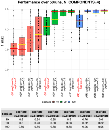
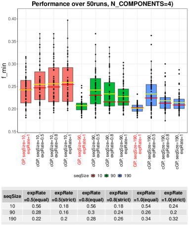
Figure 3.9: (a) The box plot of $f_{\max}$ with y-scale $(0.5,1.2)$ and (b) $f_{\min}$ with y-scale $(0.1,0.8)$ from sequential samples of 50 fitted surrogate models of piston simulation function, each dot in the box plot represents the optimal point in each run (hence each box plot contains 50 points). The sequential sample size varies from 10 to 190 with 10 pilot samples. Exploration rates of the cGP model are chosen to be 0.5, 0.8 and 1. We also show the sample mean (yellow horizontal bar) and median (red horizontal bar) among 100 optima points.

In the table at the bottom of Figure 3.9 we provide a similar quantitative comparison for GP and cGP surrogates. The fraction of out-performing batches shows that the cGP with a high exploration rate is preferred when looking for $f_{\max}$. Although the quantitative percentage does not favor cGP when searching for $f_{\min}$, by comparing the sample means and medians obtained from GP and cGP, the claim that cGP does not give a much worse $f_{\min}$ is supported. This kind of trade-off is common in choosing different surrogates. It is worth pointing out that cGP models can have a significant gain like this even if a real “non-smoothness” does not occur. It is not hard to

3.2.2.2 SuperLU_DIST parallel tuning ($d=4$). The second high-dimensional application we are studying is the tuning problem arising in the distributed-memory parallel sparse LU factorization of SuperLU_DIST (Yamazaki and Li, 2012). SuperLU_DIST is a numerical software package developed for LU factorization of large sparse matrices in parallel. There are several mechanisms introduced to speed up the LU factorization for large matrices. We use 8 Haswell nodes with 32 cores on each node, and 256 MPIs in total. This tuning problem has 4 tunable parameters, LOOKAHEAD (number of lookahead panels used to overlap the communication with computation), nprow (number of row processes out of 256 MPI processes), NSUP and NREL (parameters defining sizes of the so-called supernode representations). There are other categorical parameters COLPERM (different ways of permuting the columns) etc., for which we take the default paramter values of SuperLU and do not tune in this example.

All of these parameters are integers, and so we need to round them to the nearest integer when fitting the surrogate model over a continuous domain. The black-box objective function $f$ in this tuning problem is the running time of LU factorization for a given matrix; our examples arise in chemistry. In Table 3.3 and Figure 3.10, we display the approximate time range for the LU factorization when cGP explores the 4-parameter space with different parameter configurations, the details of these matrices are available at https://sparse.tamu.edu/PARSEC.

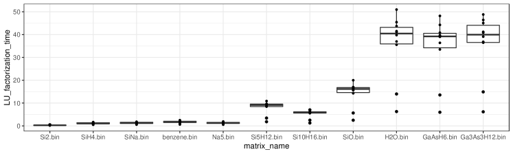
Figure 3.10: Box plots for LU factorization time when 4 parameters in the SuperLU application are randomly chosen with the same random number generator. To reduce randomness, we repeat 10 times for each parameter configuration and use the average value for each point in each column.

Size of raw data file Matrix dimension ($d\times d$ square matrices) Number of nonzeros entries in matrix Matrix name Approximate range of factorization times (seconds) GP baseline factorization time (seconds) 224Kb $769$ 17801 Si2 $\approx$ 0.10-0.90 0.145 2.0Mb $5041$ 171903 SiH4 $\approx$ 0.20-2.0 0.283 2.3Mb $5743$ 198787 SiNa $\approx$ 0.20-2.0 0.311 2.9Mb $8219$ 242669 benzene $\approx$ 0.30-4.0 0.362 3.6Mb $5832$ 305630 Na5 $\approx$ 0.20-3.0 0.285 8.6Mb $19896$ 738598 Si5H12 $\approx$ 1.0-14.0 1.136 11Mb $17077$ 875923 Si10H16 $\approx$ 0.6-8.0 0.698 16Mb $33401$ 1317655 SiO $\approx$ 2.0-22.0 1.992 26Mb $67024$ 2216736 H2O $\approx$ 5.5-53.0 5.686 39Mb $61349$ 3381809 GaAsH6 $\approx$ 5.0-55.0 5.207 36Mb $61349$ 5970947 Ga3As3H12 $\approx$ 5.0-65.0 5.382

Table 3.3: The fixed matrices (stored in raw text files with the size indicated in bytes) considered in the SuperLU_DIST application and their typical factorization time (without tuning) on 8 cori Haswell nodes, with 32 cores used on each node. We consider those matrices smaller than 10Mb as “small” while the others “large”. We also include baseline execution time when the application is tuned by a simple GP surrogate.

As above, we fix the random seed to ensure the pilot samples are the same for each surrogate model. Even with the same random seed, the running time has some noise due to the working condition of each node. In our experiments, we use the DGM classifier with the maximal number of components $k$=2, 4 and expRate=0.5, 0.8, 1.0 for the cGP model and compare their performance against the simple GP surrogate model. In this application, we want to find an optimal configuration of the SuperLU_DIST application so that the minimum running time $f_{\min}$ becomes as small as possible. $f_{\max}$ is not relevant in this application.

In Figure 3.11, we show the performance of GP and cGP surrogate models. In these applications, the choice of the maximal number of components affects the result. For matrices smaller than 10Mb, we can see that cGP can provide configurations of SuperLU_DIST that are faster than using the GP surrogate. cGP is usually not much worse than GP except when in the Na5 matrix (but its absolute value is also close). Therefore, we can use cGP in place of GP without much worry about getting a much worse $f_{\min}$. For matrices larger than 10Mb, the noise in the running time is negligible, and we observe that cGP is generally producing a better factorization time with only a few exceptions. The improvement can be as much as 7% (7.3% for GaAsH6 matrix). Again, we expect that when cGP is giving a worse result (e.g., Si10H16 matrix), it is within a 7% margin and for a better choice of exploration rate (1.0, the number of components $k=2$), we can achieve a 5% improvement. Such an improvement is quite important when we often need to conduct LU factorization multiple times.

The geometries of the objective function in both piston and SuperLU_DIST applications are not known to us. And it is hard to explore the true geometry as we did for the one-dimensional matmul application. However, we show the power of cGP by simply choosing a few different cGP surrogate models. In the piston application, we can see that $f_{\max}$ is much improved while $f_{\min}$ only loses slightly. In the SuperLU_DIST application, we can see that $f_{\min}$ gets improved over GP results very frequently, and again it would not lose by a large margin.

Figure 3.11: In the top panel, we show the absolute SuperLU_DIST running time ($f_{\min}$) obtained by each specific surrogate model with 190 sequential samples and 10 pilot samples in one run. In the bottom panel, we show the relative ratio ($f_{\min}$ obtained by certain cGP models divided by the $f_{\min}$ obtained by simple GP) of SuperLU_DIST running time obtained by each specific surrogate model against the one using simple GP surrogate model, ratios that are less than 1 means better performance. Further results can be found in Appendix D.

4 Discussion

4.1 Contribution

In this paper, we start with a comprehensive literature review of recent progress in Bayesian optimization. By a thorough review and practical experience, we identify the non-smoothness problem in the tuning context. For tuning problems, we usually have limited samples and tune more than one or two parameters. The non-smoothness problem is more challenging when we have limited samples and relatively high dimensionality. This specific problem has not been treated nor explored to the best of our knowledge, but arises in the tuning context.

To address this potential problem in the tuning context, we propose a new clustering-based method that potentially improves surrogate modeling for non-smooth black-box objective functions, which extends to high-dimensional domains without much increase in complexity. The accompanying algorithm with acquisition re-weighting is a parsimonious but novel way to fit an additive GP model by automatically creating partitions, which can be utilized in the Bayesian optimization and more general online contexts.

The cGP surrogate model works well when the black-box function shows non-smoothness or even changes sharply near the optima. When we have a clear knowledge of the underlying geometry of the problem, this knowledge usually helps us to choose the parameters of cGP surrogate models to attain better results (e.g., Bunkin N.6 in Figure 3.4). However, even when we do not know the objective functions for certain applications, cGP may help us to identify the geometry (e.g., matmul in Section 3.2.1). Even if we do not care about the geometry of the objective function, we can usually get improvement in our tuning task (e.g., piston, large matrices in SuperLU_DIST in Section 3.2.2). In the least favorable situation, using cGP would not lose much in tuning tasks compared to GP (e.g., small matrices in SuperLU_DIST).

The cGP model usually has a computational advantage over GP since it fits multiple smaller GP components instead of one large GP. This advantage is more obvious when we have a lot of samples to feed the surrogate model. When we have a bigger computational budget and many samples (as opposed to limited and sequential samples), a cGP is $k^{2}$ times (where $k$ is the number of clusters in the cGP model) faster than a GP with the same number of samples (assuming the clusters are roughly the same size). In addition, cGP can be considered as a generalization of the GP model, when we choose the maximal number of components to be 1, cGP reduces to the GP model. In this sense, cGP can be a standalone modeling method that incorporates the change-surface detection within a Bayesian framework as well. Further extensions to the sparsified versions are possible.

In terms of the partitioning induced by the cluster-classify step, we connect the sample points with the underlying black-box function in a novel way, which opens the door to more sophisticated designs to explore properties of black-box functions using sequential samples.

4.2 Future work

Considering the high flexibility of the cGP surrogate model, we can refine cGP in several natural ways. From a Bayesian perspective, it would be natural to insert a prior mechanism to allow different kinds of acquisition functions in cGP sequential sampling, potentially a different weighting of clustering components with apriori information. This may require us to modify the current cGP model into a fully Bayesian framework which exceeds the scope of the current paper. The cGP model could also be extended to multiple-output scenarios, where we may learn the partition from multiple similar runs of the application.

Proposed as an additive model, we may want to allow different covariance kernels for different components (or adaptive choice of kernels) induced by the cluster-classify step in our algorithm. Combined with the current implementation, we are able to parallelize the fitting of cGP, since the components are conditionally independent.

One practical issue is to determine the hyper-parameters used for the cGP model. For instance, we need to pick an appropriate number of components in the cGP model. One future direction is to develop a refined way of determining the number of additive components in our surrogate model. The typical cross-validation approach would not work here when there is non-smoothness, because we need to know the “correct partition” to create an appropriate training and testing set that are sampled from different regions in a balanced way. Potentially, we need an algorithmic multi-level approach: at the coarse level we use a small number of samples to bound the number of components and pin down the number of components.

It is of theoretic interest how GP surrogate models work in conjunction with non-stationary and/or compactly supported covariance kernels in the tuning context. And it is also of theoretic interest whether the clustering and classification consistency would be ensured when we have a lot of sequential samples, although we have experimental results showing good large-sample behavior Or in other words, how many samples are needed to recover the “true partition of the black-box function”? In the tuning context, an error bound for early stopping may be of more practical interest. Besides, replacing the simple GP model with more sophisticated models like deep GP (Damianou and Lawrence, 2013) would introduce another question: how can the trade-off between the number of model parameters and the number of sequential samples be balanced when we have limited samples for modeling?

One potentially more general approach is to choose different acquisition functions and exploration rates for different partition components adaptively. It is of interest to know how this relatively heuristic approach performs against the more sophisticated approach like optimization-based decomposition (Park et al., 2011). And we also intend to develop new clustering criteria that fits into the cGP framework. For instance, let each sample point $(\bm{x},y)$ be a vertex in a graph with edge weights equal to the reciprocal of a difference metric like $1/(\|\bm{x}_{1}-\bm{x}_{2}\|+\xi\cdot|y_{1}-y_{2}|)$. Then we only keep those edges with large enough weights to form a graph-based clustering, so only “nearby” vertices representing “no jumps” (i.e., smoothness) are connected. The cGP model with the cluster-classify mechanism could leverage the (graph-based) convex clustering as a potential clustering algorithm (Sun et al., 2021).

Following the consideration of a different clustering method, a natural and important future direction for addressing non-smoothness in surrogate modeling is to consider higher order non-smoothness. In Definition 1, we are motivated by non-existence of the first-order gradients of black-box functions in an open neighborhood. We expect that higher order non-smoothness motivated by higher order gradients is more complicated and so will be efforts to model that kind of non-smoothness. And the incorporation of both geometric and topological information conveyed by the non-smooth features of the black-box function may assist our modeling further (Luo and Strait, 2019).

Another main question we have not touched in the current paper is the handling of categorical (or binary) variables in the tuning context. More often than not, high-performance computing applications bring categorical variables without explicit ordering (e.g., different kinds of algorithms used for a specific optimization problem). When there are few categories involved, we build separate surrogate models for each of these categories. However, it is still of interest how we could model non-smoothness in a tuning problem where many categorical variables with multiple categories involved. In addition, we can also view the choice of clustering and classification algorithms as a categorical variable.

To summarize, we have identified a rarely explored practical problem, proposed and implemented a novel algorithm that generalizes the classical GP surrogate model. This cGP model has the ability to handle non-smoothness and complex geometry of the objective black-box function with limited online samples. We provide evidence how this model outperforms the simple GP surrogate model for high and low dimensional functions, and discuss its flexibility and possible extensions.

4.3 Ethics Compliance

• Code and data availability
  We stored our code at https://github.com/hrluo/cGP for reproducibility and production purposes. For the SuperLU_DIST application, we use the embedded code stored at https://github.com/gptune/GPTune as part of GPTune project and the SuperLU software available at https://github.com/xiaoyeli/superlu_dist.

• Acknowledgment/Funding source
  We thank Giulia Guidi for providing us the C++ code for the matmul application and helpful comments.

  This research was supported by the Exascale Computing Project (17-SC-20-SC), a collaborative effort of the U.S. Department of Energy Office of Science and the National Nuclear Security Administration. We used resources of the National Energy Research Scientific Computing Center (NERSC), a U.S. Department of Energy Office of Science User Facility operated under Contract No. DE-AC02-05CH11231.

A cGP Algorithm

Data: $X_{n_{0},d}$ (data matrix consisting of pilot samples in $H^{d}$)

Input: $X_{new}$ (data matrix of predictive locations in $H^{d}$), $k$ (optional, the number of clusters), $\tau$, (the exploration rate), $maxSampleSize$ (the maximal number of samples that can be drawn from $f$)

Result: list $g$ of GP surrogate model components corresponding to clusters

Prediction of clustered GP surrogate model at predictive locations $X_{new}$

GP ($X_{n,d},Y_{n}$) is a Gaussian process surrogate model fitted with the data matrix $X_{n,d}$ and response $Y_{n}$.

EI ($x$,$g$) is an acquisition function based on the surrogate model $g$, evaluated at $x\in H^{d}$.

CLUSTER ($X_{n,d}$,$Y_{n}$,$k$) is a (e.g., $k$-means) clustering method performed on $X_{n,d},Y_{n}$ that returns the labels of a data matrix $X_{n,d}$ as an $n\times 1$ vector.

CLASSIFY ($X_{n,d}$,$(X^{{}^{\prime}}_{n^{\prime},d},L^{{}^{\prime}}_{n^{\prime},1})$) is a (e.g., $k$-nearest neighbors) classification method that is trained by a set of labeled data $(X^{{}^{\prime}}_{n^{\prime},d},L^{{}^{\prime}}_{n^{\prime},1})$; and returns the labels of a data matrix $X_{n,d}$ as an $n\times 1$ vector.

uni ($v$) is a function that returns unique values in the vector $v$.

1begin

      2 $X$ = $X_{n_{0},d}$

       while $i<maxSampleSize$ do

            

            3Generate a random number $u\in[0,1]$

             if $u\leq\tau$ then

                  4 $g$ = $[\cdots]$; $x0$ = $[\cdots]$; $ei0$ = $[\cdots]$

                  

                  5$dataLabel$ = CLUSTER ($X$,$k$); $clusLabel$ = uni ($dataLabel$)

                   /* fit the clustered GP surrogate model with $X$ = $X_{n_{0},d}$ */

                  

                  /* In practice, we also eliminate those clusters with too small sizes to avoid mis-fits. */

                   for j in $clusLabel$ do

                        6 $X_{j}$ = $X[dataLabel==j,:]$

                        7 $Y_{j}$ = $Y[dataLabel==j]$

                        8 $g[j]$ = GP ($X_{j}$,$Y_{j}$)

                        9 $x0[j]$ = $\arg\max_{x\in H^{d}}$EI ($x$,$g[j]$); $ei0[j]$ = EI ($x0[j]$,$g[j]$)

                         /* The CLASSIFY ($\bm{x}$,$(X,dataLabel)$ is implicitly used in this step. */

                        

                   end for

                  10$j0$ = $\arg\max_{j\in clusLabel}ei0[j]/|dataLabel==j|$

                   /* weighted acquisition function by cluster size */

                  11 Append $x0[j0]$ and its function values $f(x0[j0])$ to the $X$ and $Y$

            

            else

                  12 Append random location $x1$ and its function values $f(x1)$ to the $X$ and $Y$

             end if

            

       end while

      /* predict based on the fitted clustered GP surrogate model */

      13 $dataLabel$ = CLUSTER ($X$,$Y$,$k$)

       for $\bm{x}\text{ {in} }X_{new}$ do

            14 Find the label CLASSIFY ($\bm{x}$,$(X,dataLabel)$) and let $j_{\bm{x}}$ = the $dataLabel$ of $\bm{x}$

            15 Predict the value of surrogate function at $\bm{x}$ using GP model $g[j_{\bm{x}}]$

       end for

      

end

Algorithm 1 Clustered Gaussian process (cGP) surrogate model algorithm (the algorithm that carries out the idea described in Sec. 2)

B Additional Synthetic Studies

In this set of experiments, we pick a set of 2-dimensional benchmark functions. For each of these functions, we know the exact minimum from its expression. However, these analytical solutions are designed to be difficult to find by popular optimization methods. We would briefly describe the function at the beginning of each section and display its minima. Among all these well-known benchmark functions, practitioners only concern about minima. We do not have to consider maxima, as suggested in most benchmarks. In addition, there is a typical domain for these benchmark functions, over which people would like to search for minima.

For each run, we assume that we always have 10 randomly chosen pilot samples (it turns out that the optimal design would not systematically help in synthetic function cases). In addition, we choose three different sample sizes: 10 (limited sample size), 90 (normal sample size) and 190 (abundant sample size). The major factor we tune for cGP model is the number of components ($k=2,3,4$), which is the maximal number of components allowed in the cGP model. We use DGM cluster algorithm to decide clustering labels; and k-NN $(k=3)$ to decide the classification labels. For each random seed, we have the same set of 10 pilot samples, and fit GP model, cGP models (with N_SEQUENTIAL 10, 90, 190). For each sample size, we also adjust the expRate of the cGP model as 0.5, 0.8 and 1.0. Therefore, we would have $3\times 3=9$ different cGP models against one GP model for a fixed sample size.

The first comparison is the violin plot, a generalization of the box plot. The violin plot shows 10%, 25%, 50%, 75%, 90% quantiles of the estimated density of 100 minima obtained by each surrogate model among 100 runs, with black solid lines. We also show the sample mean (yellow horizontal bar) and median (red horizontal bar) among 100 points. In the violin plot, we can see the estimated density of surrogate minima as the sequential sample size increases. In addition, since minima are displayed as a distribution of dots in the plot, we can avoid the delusion of a good single run and see the systematic performance of a specific surrogate model against another model. When we see a significantly lower clump, we can conclude that the cGP model is distributionally better than the GP model. This shows a significant trend and eliminates the randomness in single runs as much as possible.

The second comparison is the percentage table, as we have seen in Figure 3.4. The table includes two types of percentage. The “(equal)” percentage means the percentage of batches that the corresponding cGP models give an equal or smaller minimum among all sequential samples drawn. The “(strict)” percentage means the percentage of batches that the corresponding cGP model gives strictly smaller minima among all sequential samples drawn. When we see (equal) greater than 50% and (strict) greater than 1-(equal)%, we can conclude that there is a significant advantage of using cGP (with an appropriate setting). This means that at least half of times cGP outperforms or equal to GP; and cGP performs better more often than GP.

1. The Bukin N.6 function has an expression $f(x)=100\sqrt{|x_{2}-0.01x_{1}^{2}|}+0.01|x_{1}+10|$. The function has four global minima $f(x_{\ast})=0$ at $x_{\ast}=(-10,1)$. We optimize over $[-15,5]\times[-3,3]$.
   

   
   

2. The Easom function has an expression $f(x)=-\cos(x_{1})\cos(x_{2})\exp(-(x_{1}-\pi)^{2}-(x_{2}-\pi)^{2})$. The function has four global minima $f(x_{\ast})=-1$ at $x_{\ast}=(\pi,\pi)$. We optimize over $[-10,10]\times[-10,10]$.
   

   
   

3. The Michalewicz function has an expression $f(x)=-\sin(x_{1})\sin^{20}\left(\frac{x_{1}^{2}}{\pi}\right)-\sin(x_{2})\sin^{20}\left(\frac{2x_{2}^{2}}{\pi}\right)$. The function has four global minima $f(x_{\ast})=-1.8013$ at $x_{\ast}=(2.20,1.57)$. We optimize over $[0,4]\times[0,4]$.
   

   
   

4. The Schaffer N.2 function has an expression $f(x)=0.5+\frac{sin^{2}(x_{1}^{2}-x_{2}^{2})-0.5}{\left[1+0.001\cdot(x_{1}^{2}+x_{2}^{2})\right]^{2}}$. The function has four global minima $f(x_{\ast})=0$ at $x_{\ast}=(0,0)$. We optimize over $[-2,2]\times[-2,2]$.
   

   
   

5. The Holder Table function has an expression

   $$f(x)=-\left|\sin(x_{1})\cos(x_{2})\exp\left(\left|1-\frac{\sqrt{x_{1}^{2}+x_{2}^{2}}}{\pi}\right|\right)\right|.$$ (5)

   The function has four global minima $f(x_{\ast})=-19.2085$ at $x_{\ast}=(\pm 8.05502,\pm 9.66459)$. We optimize over $[-10,10]\times[-10,10]$.
   

   
   

6. The Cross-in-Tray function has an expression

   $$f(x)=-0.0001\left(\left|\sin(x_{1})\sin(x_{2})\exp\left(\left|100-\frac{\sqrt{x_{1}^{2}+x_{2}^{2}}}{\pi}\right|\right)\right|+1\right)^{0.1}.$$ (6)

   The function has four global minima $f(x_{\ast})=-2.06261218$ at $x_{\ast}=(\pm 1.3494,\pm 1.3494)$. We optimize over $[-10,10]\times[-10,10]$.
   

   
   

Based on the results of the synthetic studies we obtained from these benchmark functions, the following empirical observations are made:

1. If the black-box function has optima hidden in a “slit-like” (low-dimensional and also near dis-continuous) region, then cGP produces better and faster results, along with a nice partition scheme (Bukin N6 as in Figure 3.4 and Easom).

2. In some situations where the black-box function is smooth, cGP could still show competitive performance using several smaller GP components. It could also be tuned to show better tail behavior in the sense that the obtained minima are closer to the truth more often (Michalewicz).

3. If the black-box function has a noisy and rough surface, then cGP can be configured to perform as good as GP, usually faster, and come up with clustering regimes. (Schaffer N2)

4. If the black-box function has optima in a relatively small region compared to the whole domain, then cGP may not produce very informative regimes (Easom and Holder Table) but it would reach better optima; and runs faster.

5. If the true function has significant dis-continuities and relatively strong signal (matmul with averaging), then cGP can identify different regimes rather faithfully. The common feature of those function where cGP outperforms GP is that the function changes sharply (hence analogous to a non-smoothness) near the minimum.

C Additional Results of Experiments in Section 3.2.1

Besides the problem setting of changing block size in the matmul application, we can also fix and optimize our blocking strategy but test the optimized blocking strategy with different matrix sizes. In this experiment, when the matrix size exceeds the memory cache size, the computational speed would experience an immediate drop, as we would observe in Figure C.1 below. The black-box function $f$ in this application is still computational speed, but the tuning variable $\bm{x}$ is the matrix size.

All of their cache-line sizes are 64 bytes, equivalent to 8 double precision floating point numbers. Based on this consideration, we can sample the block sizes $b$ that are multiples of 8 in this example.

(a)	(b)
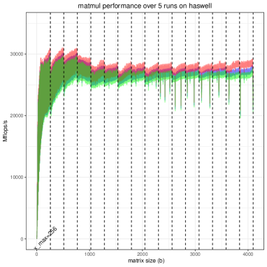
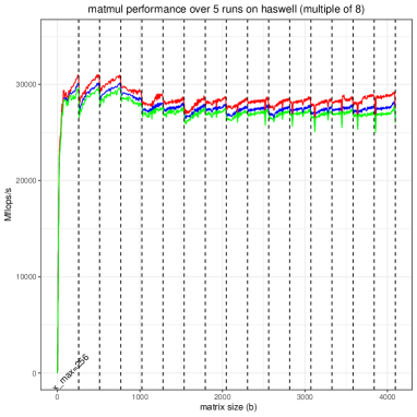
$\bm{x}_{\text{max}}=256$	$\bm{x}_{\text{max}}=256$

Figure C.1: The computational speed for matrices of sizes varying from $16$ to $4096$. The red line shows the maximum among 5 runs; the green line shows the minimum among 5 runs; the blue line shows the average among 5 runs. (a) The matrix size varies from 16 to 4096, obtained from 5 different runs. (b) The matrix sizes are multiples of 8, varying from 16 to 4096. We also use dashed lines to indicate the matrix sizes that are multiples of 256 where we expect a drop by machine architecture.

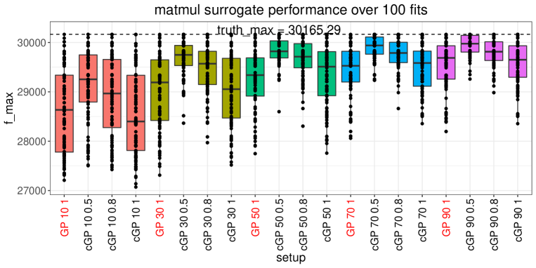
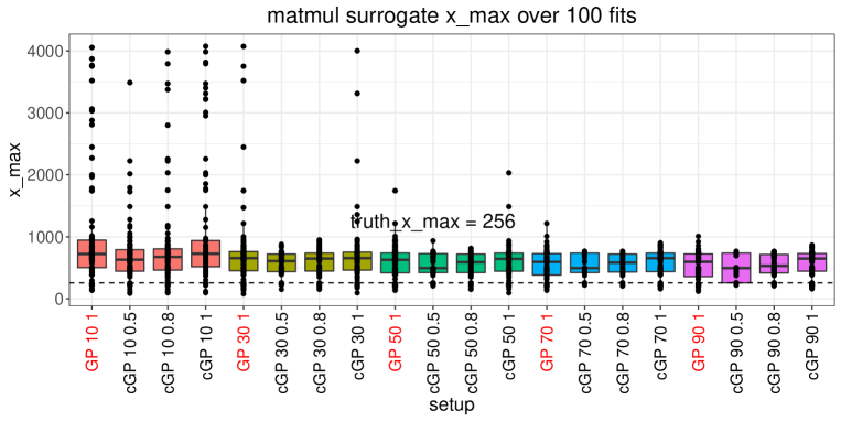
Figure C.2: The box plot of $f_{\max}$ (top) and $\bm{x}_{\max}$ (bottom) elicited from sequential samples of 100 fitted surrogate models, each dot in the box plot represents the optimal point in each run (hence each box plot contains 100 points). The sequential sample size varies from 10 to 190 with 10 pilot samples. The exploration rates of the cGP model are chosen to be 0.5, 0.8 and 1.
Results for simple GP surrogates are highlighted with red labels as a baseline surrogate model; while cGP surrogates with different exploration rates are highlighted with black labels.

To eliminate the randomness caused by a single run, we repeat cGP (and GP) for 100 different random seeds with 10 pilot random samples for each run. In Figure C.2, we compare the performance of a simple GP surrogate model searching over any integer $[16,4096]\cap\mathbb{Z}$ against our cGP model with the exact number of components 3 (with $k$-means clustering) and $k=3$ in the k-NN classification step (See Figure 2.1). Our cGP model searches over integers that are multiples of 8 over $[16,4096]$. Qualitatively, it is not hard to see that cGP performs better than the GP model, under almost all sample sizes.

In this matrix multiplication example with varying matrix sizes, the cause of non-smooth points (i.e., reduction of communication; overflow of fast cache) and different kinds of behavior are clear and observed in the recorded dataset as shown in Figure C.1. Our optimized strategy would attain the best performance on the matrix with matrix size $\bm{x}_{\max}=256$. In the summary Figure C.2, cGP surrogates behave similarly to the GP model when there are few samples; but when there are enough samples, the cGP model clearly identifies different partition regimes much better with a reasonable accuracy improvement. Therefore, the cGP model searches the optimum $f_{\max}$ and $\bm{x}_{\max}$ more efficiently compared to a simple GP surrogate, with more evidence shown in Table C.1.

		(a)			(b)			(c)
Exp. rate		1.0	0.8	0.5	1.0	0.8	0.5	1.0	0.8	0.5
Sample size	$n=10$	0.57	0.69	0.78	2	2	2	1.79	1.85	1.83
	$n=30$	0.65	0.74	0.82	3	3	5	2.08	2.10	2.20
	$n=50$	0.67	0.74	0.85	4	5	9	2.15	2.20	2.27
	$n=70$	0.62	0.74	0.82	4	6	11	2.24	2.31	2.38
	$n=90$	0.61	0.70	0.80	4	7	12	2.30	2.37	2.38

Table C.1: (a) The percentage of cGP fitted surrogates with optima equal or better than the baseline GP surrogate under different exploration rates. (b) The number of cGP fitted surrogates that attain the actual optimal matrix size $\bm{x}_{\max}=256$ under different exploration rates. A simple GP surrogate model would only reach $\bm{x}_{\max}=256$ once in 100 different random seeds. (c) The average number of additive components in the fitted cGP surrogate models among 100 different random seeds.

To better understand the performance behavior, we provide cache-miss profiling results of the matrix multiplication for varying matrix sizes. We used Linux’s Perf to collect the cache miss rates. The profiling results show that the cache miss rate at each cache level has a jump when exceeding a certain matrix size.

We show the peak performance and cache traffic for only one execution of the matmul application. The execution is done on the same node type with the Haswell architecture as mentioned in Sec. 3.2.1. We obtain the data read/load traffic of L1 (Data cache, 32KB), L2 (Unified cache, 256KB) and L3 (Unified cache, 40960KB; also known as LLC, last layer cache) cache.

Theoretical calculations concerning only whether matrices fit into storage show that, ideally, the matrix size that makes the matrices exceed the L1 ($\approx$52), L2 ($\approx$105) and L3 ($\approx$1322) caches (using $\sqrt{\frac{1}{3}\text{cache bytes}/8}$ for accessing three double precision square matrices in the matmul application.) These threshold matrix sizes are illustrated by blue vertical lines in the Figure C.3.

The statistic we monitor is the cache miss rate. For L1 cache, we monitor the data load miss rate; for L2 cache, we monitor the data demand miss rate and all demand miss rate; for L3 cache, we monitor the data load, store miss rates and their sum. These hardware measurements lend support to our claim that the black-box function $f$ does have some non-smoothness and partially explain why the partition obtained by the cGP model is beneficial. It also partially validates the findings of surrogate models in the tuning context. By incorporating the non-smoothness in the tuning context, our model also induces informative partitions consistent with non-smoothness observed in the profiling.

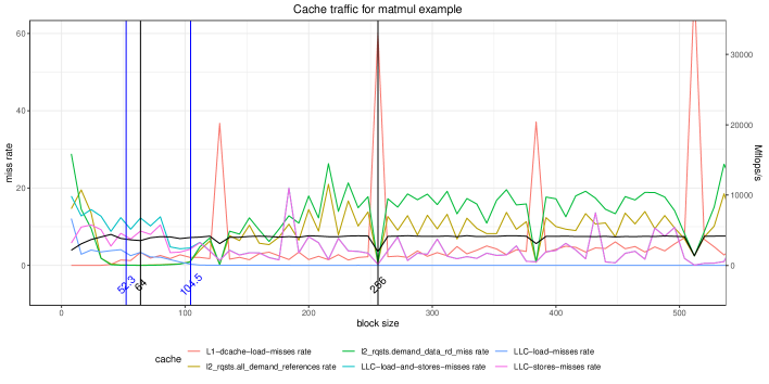
Figure C.3: Cache traffic and computational performance for one batch of the matmul application. The top panel shows the traffic when the block size changes among multiples of 8 from 10 to 4096; the bottom panel shows a zoom-in version of the top panel focusing on the traffic for block size less than 512. The x-axis is the block size in the matmul application. The left y-axis is the percentage of miss rate for each type of cache. The right y-axis is the computational speed of the matmul application.

D Additional Results of Experiments in Figure 3.11

The following figures are organized in the same formats: In the top panel, we show the absolute SuperLU_DIST running time ($f_{\min}$) obtained by each specific surrogate model with different number of sequential samples and 10 pilot samples in one run. In the bottom panel, we show the relative ratio ($f_{\min}$ obtained by cGP models divided by the $f_{\min}$ obtained by simple GP) of SuperLU_DIST running time obtained by each specific surrogate model against the one using the simple GP surrogate model, ratios that are less than 1 means better performance.

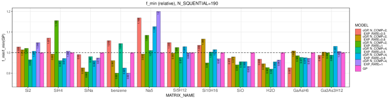
Figure D.1: SuperLU_DIST results with 10 pilot and 10 sequential samples.

Figure D.2: SuperLU_DIST results with 10 pilot and 90 sequential samples.

E Theoretic Results

Let us start with a simpler situation by supposing the partitions of components are fixed from the beginning of sequential sampling.

Assumption A. The number of components $k<\infty$ is known and cannot change.

To ensure the convergence of the surrogate model, we need to assume that the covariance kernel $K$ satisfies:

Assumption B. The Fourier transform $\hat{K}(\bm{\xi})\coloneqq\int_{\mathbb{R}^{d}}2^{-2\pi i\left\langle\bm{x},\bm{\xi}\right\rangle}K(\bm{x})d\bm{x}$ exists, is isotropic and non-increasing and satisfy either $\hat{K}(\bm{\xi})=\Theta\left(\|\bm{\xi}\|^{-2\nu-d}\right)$ for some $\nu>0$ or $\hat{K}(\bm{\xi})=O\left(\|\bm{\xi}\|^{-2\nu-d}\right)$ for $\forall\nu>0$ (and denote $\nu=\infty$). We call this $\nu$ the smoothness parameter of the covariance kernel $K$. (Assumption B is exactly the Assumptions 1,2 and 3 in Bull (2011))

Assumption C. The covariance kernel $K$ is $\mathcal{C}^{\left\lceil 2\nu\right\rceil}$ and the $\left\lceil 2\nu\right\rceil$-th order Taylor approximation $P_{K}$ satisfy $\left|K(\bm{x})-P_{K}(\bm{x})\right|=O\left(\|\bm{x}\|^{2\nu}\left(-\log\|\bm{x}\|\right)^{2\alpha}\right)$ as $\bm{x}\rightarrow 0$ for some $\alpha\geq 0$. (Assumption 4 in Bull (2011))

Both Matern family and exponential kernel satisfy Assumption 2 and 3 above. When the partitions are fixed, the crucial condition of the convergence of GP surrogate lies in the regularity of the component domains and the sample size. The regularity of the component domain can be described by

Definition 2

(Lipschitz domain, Wynne et al. (2021)) An open set $\mathcal{X}_{i}\subset\mathbb{R}^{d}$ is called a (special) Lipschitz domain if there exists a rotation of $\mathcal{X}_{i}$, denoted by $\bar{\mathcal{X}}_{i}$, and a function $\psi:\mathbb{R}^{d-1}\rightarrow\mathbb{R}$ which satisfies the following:

(1) $\mathcal{X}_{i}=\{(x,y)\in\mathbb{R}^{d},y>\psi(x)\}$

(2) $\psi$ is a Lipschitz function such that $\left|\psi(x)-\psi(x^{\prime})\right|\leq M\|x-x^{\prime}\|_{2}$ for any $x,x^{\prime}\in\mathbb{R}^{d-1}$ and some $M>0$.

For instance, the binary divisions adopted by Chipman et al. (2010) consist of Lipschitz domains with piecewise constant functions $\psi=c_{j}$.

Proposition 3

Suppose Assumptions A hold and that the domain $\mathcal{X}$ can be decomposed into Lipschitz domains $\mathcal{X}_{1}\cup\cdots\cup\mathcal{X}_{k}=\mathcal{X}$ and each $\mathcal{X}_{j}$ is compact with an nonempty interior. In the reproducing kernel Hilbert space (RKHS) $\mathcal{H}_{\theta}(\mathcal{X})$ defined by the covariance kernel $K_{\theta}$ on $\mathcal{X}$, let us suppose that black-box functions $f\mid_{\mathcal{X}_{j}}\in\mathcal{H}_{\theta_{U}}(\mathcal{X}_{j}),j=1,\cdots,k$ with $\theta\leq\theta_{U}<\infty$ satisfy Assumption B and C. Then there exists an integer $n_{0}>k$ such that the interpolant optimum (Bull, 2011) $\bm{x}_{n}^{*}$ satisfy

$$\sup_{\begin{array}[]{c}\|f\|_{\mathcal{H}_{\theta^{U}}(\mathcal{X}_{j})}\leq R\\ j=1,\cdots,k\end{array}}\mathbb{E}_{f}\left|f(\bm{x}_{n}^{*})-\min_{\mathcal{X}}f\right|=O\left(\left(\frac{n}{\log n}\right)^{-\nu/d}\left(\log n\right)^{\alpha}\right)$$ (7)

for some $R>0$ and all sufficiently large sample size $n>n_{0}$. If $\nu=\infty$ then the statement holds for all $\nu<\infty$.

Proof. The idea of the proof is that the overall sequence $\bm{x}_{1},\bm{x}_{2},\cdots,\bm{x}_{n}$ of sequential sampling can be organized into sub-sequences for each component, which grow simultaneously due to our algorithm. Within each component we have an asymptotic scheme, the regularity of the component domains allow us to apply results in Bull (2011) obtained from the RKHS techniques for each component.

The sequential samples $\bm{x}_{1},\bm{x}_{2},\cdots,\bm{x}_{n}$ are chosen from one of all $k$ independent components in the additive GP model. Therefore, if we use the super script to denote the component a sample point belongs to, we can reorganize the sample sequence $\bm{x}_{1},\bm{x}_{2},\cdots,\bm{x}_{n}$ into $k$ sub-sequences where the sizes of sub-sequences satisfy $n_{1}+\cdots+n_{k}=n$:

$$\bm{x}_{1}^{(1)},\bm{x}_{2}^{(1)},\cdots,\bm{x}_{n_{1}}^{(1)} ;\quad\bm{x}_{1}^{(2)},\bm{x}_{2}^{(2)},\cdots,\bm{x}_{n_{2}}^{(2)}\quad\cdots \bm{x}_{1}^{(k)},\bm{x}_{2}^{(k)},\cdots,\bm{x}_{n_{k}}^{(k)}.$$

Now we also need to show that all $n_{1},n_{2},\cdots,n_{k}>1$ and tend to infinity, for otherwise, there would be components containing no sequential sample points at all. However, this cannot happen, due to the fact that overall sequential sampling strategy is to pick the maximizer of EI acquisition function $\text{EI}_{j}(\bm{x})$ in each component weighted by component sample size $n_{j}$. If $n_{1}=1$ while $n_{2},\cdots,n_{k}>1$ then we can pick $n_{0}$ such that

$$\frac{\max_{j=2,\cdots,k}\max_{\bm{x}\in\mathcal{X}_{j}}\text{EI}_{j}(\bm{x})}{\min(n_{2},\cdots,n_{k})+n_{0}/(k-1)}\leq\max_{\bm{x}\in\mathcal{X}_{1}}\text{EI}_{1}(\bm{x})/1$$

The numerator is the maximal acquisition function among all $\text{EI}_{j}(\bm{x}),j=1,2,\cdots,k$, which is non-increasing by the definition of EI function. The denominator $n_{0}/(k-1)$ can be intuitively understood as each sequential sample avoiding $\mathcal{X}_{1}$ would add $1/(k-1)$ sample to each of components $2,\cdots,k$.

Alternatively, assume that there exists some $j_{0}$ such that $n_{j_{0}}\not{\rightarrow}\infty$ and bounded by $n_{j_{0}}\leq N_{0}<\infty$ as $n\rightarrow\infty$. When $n$ is large enough, the following holds since the RHS is a constant and the LHS has its denominator tending to infinity while its numerator is bounded.

$$\frac{\max_{j\in A}\max_{\bm{x}\in\mathcal{X}_{j}}\text{EI}_{j}(\bm{x})}{\min_{j\in A}n_{j}}\leq\frac{\max_{\bm{x}\in\mathcal{X}_{j_{0}}}\text{EI}_{j_{0}}(\bm{x})}{N_{0}}$$

Therefore, we can increase the sample size $n>n_{0}$, then all weighted acquisition functions from components $2,\cdots,k$ would have maxima less than the maximum of $\text{EI}_{1}(\bm{x})$. Therefore, the $(n+1)$-th sequential sample must be selected as the maximizer of $\text{EI}_{1}(\bm{x})$ in $\mathcal{X}_{1}$. Following similar arguments on $n_{j}-\min_{j}n_{j}$ , we can see that $\min_{j=1,\cdots,k}n_{j}\rightarrow\infty$ as $n\rightarrow\infty$.

When all $n_{1},n_{2},\cdots,n_{k}>0$, by our algorithm, for the sub-sequence

$$\bm{x}_{1}^{(j)},\bm{x}_{2}^{(j)},\cdots,\bm{x}_{n_{j}}^{(j)},$$

$$\bm{x}_{J}^{(j)}\coloneqq\arg\max_{\bm{x}\in\mathcal{X}_{j}}\text{EI}_{j}(\bm{x})/J,$$

for $j=1,2,\cdots,k$. It is straightforward to see that $\bm{x}_{J}^{(j)}$ is also the $\arg\max_{\bm{x}\in\mathcal{X}_{j}}\text{EI}_{j}(\bm{x})$. Due to the fact that additive components are independent, each sub-sequence constitutes a sequential sampling within the component domain $\mathcal{X}_{j}$ with the same strategy. We use the assumption on $f\mid_{\mathcal{X}_{j}}$ and apply Theorem 5 of Bull (2011) to each of these $k$ independent components ($j=1,\cdots,k$) that

$$\sup_{\|f\mid_{\mathcal{X}_{j}}\|_{\mathcal{H}_{\theta^{U}}(\mathcal{X}_{j})}\leq R_{j}}\mathbb{E}_{f}\left|f\mid_{\mathcal{X}_{j}}(\bm{x}_{n_{j}}^{(j)*})-\min_{\mathcal{X}_{j}}f\mid_{\mathcal{X}_{j}}\right|=O\left(\left(\frac{n_{j}}{\log n_{j}}\right)^{-\nu/d}\left(\log n_{j}\right)^{\alpha_{j}}\right),$$

and we take the maximum (since $k<\infty$) on the LHS to yield the stated result (7) with $\alpha=\max_{j}\alpha_{j}>0$ and $R=\min_{j}R_{j}>0$. $\square$

Our result is slightly weaker than Theorem 5 in Bull (2011) in the sense that the same claim of error in terms of the supremum norm holds for every sample size $n>0$. Our results can be applied to quite general additive GP surrogate models with mutually independent components. One step further, Wynne et al. (2021) proved that even the $\nu$ are mis-specified, the convergence may still hold with a worse rate.

This discussion reveals the effect and importance of re-weighting acquisition functions in the cGP algorithm. Assumptions B and C focus on the smoothness for $f$ within each component. This convergence would not hold if EI is not weighted, regardless the distribution assumption of $\bm{x}_{i}^{\prime}s$.

However, we shall point out that our Algorithm 1 would update the partition induced by the cluster-classify step for each sampling step. Therefore, this proposition does not cover exactly cGP, but we provide a justification for weighting acquisition functions when we use an additive model in a Bayesian optimization setting. Besides, we do observe empirically that the partition usually becomes stable after sufficiently many samples are collected, so the simplification is not groundless.

That being said, we still need to rigorously prove clustering and classification consistency (in sense that the decision boundaries coincide with non-smooth borders with an appropriately chosen $\xi$). This remains an unsolved theoretic question in the current paper, but usually a reasonable choice of $\xi$ or even $\xi=1$ can lead to empirically satisfying optimization results.

References

- Adams and MacKay (2007) Ryan P. Adams and David J. C. MacKay. Bayesian online changepoint detection. arXiv:0710.3742 [stat], 2007.
- Barry and Hartigan (1993) Daniel Barry and J. A. Hartigan. A bayesian analysis for change point problems. Journal of the American Statistical Association, 88(421):309–319, 1993.
- Basseville and Nikiforov (1993) M. Basseville and I. V. Nikiforov. Detection of Abrupt Changes: Theory and Application. Prentice Hall Information and System Sciences Series. Prentice Hall, Englewood Cliffs, N.J, 1993.
- Bilmes et al. (1997) Jeff Bilmes, Krste Asanovic, Chee-Whye Chin, and Jim Demmel. Optimizing matrix multiply using phipac: a portable, high-performance, ansi c coding methodology. In ACM International Conference on Supercomputing 25th Anniversary Volume, pages 253–260, 1997.
- Blackford et al. (2002) L. Susan Blackford, Antoine Petitet, Roldan Pozo, Karin Remington, R. Clint Whaley, James Demmel, Jack Dongarra, Iain Duff, Sven Hammarling, Greg Henry, et al. An updated set of basic linear algebra subprograms (BLAS). ACM Transactions on Mathematical Software, 28(2):135–151, 2002.
- Booker et al. (1999) Andrew J. Booker, John E. Dennis, Paul D. Frank, David B. Serafini, Virginia Torczon, and Michael W. Trosset. A rigorous framework for optimization of expensive functions by surrogates. Structural optimization, 17(1):1–13, 1999.
- Brochu et al. (2010) Eric Brochu, Vlad M. Cora, and Nando de Freitas. A tutorial on bayesian optimization of expensive cost functions, with application to active user modeling and hierarchical reinforcement learning. arXiv:1012.2599 [cs], 2010.
- Bull (2011) Adam D. Bull. Convergence rates of efficient global optimization algorithms. Journal of Machine Learning Research, 12(10), 2011.
- Chen et al. (2012) Bo Chen, Rui Castro, and Andreas Krause. Joint optimization and variable selection of high-dimensional gaussian processes. arXiv:1206.6396 [cs, stat], 2012.
- Chipman et al. (1998) Hugh A. Chipman, Edward I. George, and Robert E. McCulloch. Bayesian CART model search. Journal of the American Statistical Association, 93(443):935–948, 1998.
- Chipman et al. (2010) Hugh A. Chipman, Edward I. George, and Robert E. McCulloch. BART: Bayesian additive regression trees. The Annals of Applied Statistics, 4(1):266–298, 2010.
- Cramér and Leadbetter (2013) H. Cramér and M.R. Leadbetter. Stationary and Related Stochastic Processes: Sample Function Properties and Their Applications. Dover Books on Mathematics. Dover Publications, 2013.
- Dai et al. (2019) Zhongxiang Dai, Haibin Yu, Bryan Kian Hsiang Low, and Patrick Jaillet. Bayesian optimization meets bayesian optimal stopping. In International Conference on Machine Learning, pages 1496–1506. PMLR, 2019.
- Damianou and Lawrence (2013) Andreas Damianou and Neil D Lawrence. Deep gaussian processes. In Artificial intelligence and statistics, pages 207–215. PMLR, 2013.
- Devroye et al. (2013) Luc Devroye, László Györfi, and Gábor Lugosi. A probabilistic theory of pattern recognition, volume 31. Springer Science & Business Media, 2013.
- Friedman (1991) Jerome H Friedman. Multivariate adaptive regression splines. The annals of statistics, pages 1–67, 1991.
- Fuchs and Garcke (2020) Barbara Fuchs and Jochen Garcke. Simplex stochastic collocation for piecewise smooth functions with kinks. International Journal for Uncertainty Quantification, 10(1), 2020.
- Garrido-Merchán and Hernández-Lobato (2020) Eduardo C Garrido-Merchán and Daniel Hernández-Lobato. Dealing with categorical and integer-valued variables in bayesian optimization with gaussian processes. Neurocomputing, 380:20–35, 2020.
- Gramacy (2020) Robert B. Gramacy. Surrogates: Gaussian process modeling, design, and optimization for the applied sciences. Chapman and Hall/CRC, 2020.
- Gramacy and Apley (2015) Robert B Gramacy and Daniel W Apley. Local gaussian process approximation for large computer experiments. Journal of Computational and Graphical Statistics, 24(2):561–578, 2015.
- Gramacy and Lee (2008) Robert B. Gramacy and Herbert K. H. Lee. Bayesian treed gaussian process models with an application to computer modeling. Journal of the American Statistical Association, 103(483):1119–1130, 2008.
- Gramacy and Lee (2011) Robert B. Gramacy and Herbert K. H. Lee. Optimization under unknown constraints. Bayesian Statistics, 9(9):1–18, 2011.
- Gramacy and Ludkovski (2015) Robert B. Gramacy and Michael Ludkovski. Sequential design for optimal stopping problems. SIAM Journal on Financial Mathematics, 6(1):748–775, 2015.
- Gramacy and Polson (2010) Robert B. Gramacy and Nicholas G. Polson. Particle learning of Gaussian process models for sequential design and optimization. arXiv:0909.5262 [stat], July 2010.
- Herlands et al. (2016) William Herlands, Andrew Wilson, Hannes Nickisch, Seth Flaxman, Daniel Neill, Wilbert Van Panhuis, and Eric Xing. Scalable gaussian processes for characterizing multidimensional change surfaces. In Artificial Intelligence and Statistics, pages 1013–1021. PMLR, 2016.
- Hernández-Lobato et al. (2014) José Miguel Hernández-Lobato, Matthew W. Hoffman, and Zoubin Ghahramani. Predictive Entropy Search for Efficient Global Optimization of Black-box Functions. arXiv:1406.2541 [cs, stat], June 2014.
- Holmström et al. (2008) Kenneth Holmström, Nils-Hassan Quttineh, and Marcus M. Edvall. An adaptive radial basis algorithm (ARBF) for expensive black-box mixed-integer constrained global optimization. Optimization and Engineering, 9(4):311–339, 2008.
- Hong and Kung (1981) Jia-Wei Hong and H. T. Kung. I/O complexity: The red-blue pebble game. In Proceedings of the Thirteenth Annual ACM Symposium on Theory of Computing - STOC ’81, Milwaukee, Wisconsin, United States, 1981. ACM Press.
- Kandasamy et al. (2017) Kirthevasan Kandasamy, Gautam Dasarathy, Jeff Schneider, and Barnabás Póczos. Multi-fidelity bayesian optimisation with continuous approximations. In International Conference on Machine Learning, pages 1799–1808. PMLR, 2017.
- Kenett et al. (2013) Ron S. Kenett, Shelemyahu Zacks, and Daniele Amberti. Modern Industrial Statistics: With Applications in R, MINITAB and JMP. John Wiley & Sons, 2013.
- Krause and Guestrin (2007) Andreas Krause and Carlos Guestrin. Nonmyopic active learning of gaussian processes: an exploration-exploitation approach. In Proceedings of the 24th international conference on Machine learning, pages 449–456, 2007.
- Lee et al. (2020) Eric Hans Lee, Valerio Perrone, Cedric Archambeau, and Matthias Seeger. Cost-aware bayesian optimization. arXiv:2003.10870 [cs, stat], 2020.
- Letham et al. (2019) Benjamin Letham, Brian Karrer, Guilherme Ottoni, and Eytan Bakshy. Constrained bayesian optimization with noisy experiments. Bayesian Analysis, 14(2):495–519, 2019.
- Luo and Strait (2019) Hengrui Luo and Justin Strait. Combining geometric and topological information in image segmentation. arXiv e-prints, pages arXiv–1910, 2019.
- Luo et al. (2020a) Hengrui Luo, Steven N. MacEachern, and Mario Peruggia. Asymptotics of lower dimensional zero-density regions. arXiv:2006.02568, pages 1–28, 2020a.
- Luo et al. (2020b) Hengrui Luo, Giovanni Nattino, and Matthew T. Pratola. Sparse Additive Gaussian Process Regression. arXiv:1908.08864 [math, stat], 2020b.
- Martinez-Cantin (2015) Ruben Martinez-Cantin. Locally-biased bayesian optimization using nonstationary gaussian processes. In Neural Information Processing Systems (NIPS) workshop on Bayesian Optimization, volume 7, page 4, 2015.
- Müller and Day (2019) Juliane Müller and Marcus Day. Surrogate Optimization of Computationally Expensive Black-Box Problems with Hidden Constraints. INFORMS Journal on Computing, 31(4):689–702, 2019.
- Nguyen et al. (2020) Vu Nguyen, Sebastian Schulze, and Michael A. Osborne. Bayesian optimization for iterative learning. arXiv:1909.09593 [cs, stat], 2020.
- Owen et al. (2014) Art B Owen, Josef Dick, and Su Chen. Higher order sobol’indices. Information and Inference: A Journal of the IMA, 3(1):59–81, 2014.
- Paciorek and Schervish (2004) Christopher J. Paciorek and Mark J. Schervish. Nonstationary covariance functions for gaussian process regression. In Advances in Neural Information Processing Systems 16, pages 273–280. MIT Press, 2004.
- Page (1954) E. S. Page. Continuous inspection schemes. Biometrika, 41(1/2):100, 1954.
- Park et al. (2011) Chiwoo Park, Jianhua Z. Huang, and Yu Ding. Domain decomposition approach for fast gaussian process regression of large spatial data sets. Journal of Machine Learning Research, 11:1697–1728, 2011.
- Park and Choi (2010) Sunho Park and Seungjin Choi. Hierarchical gaussian process regression. In Proceedings of 2nd Asian Conference on Machine Learning, volume 13 of Proceedings of Machine Learning Research, pages 95–110. JMLR Workshop and Conference Proceedings, 2010.
- Rasmussen and Williams (2006) Carl Edward Rasmussen and Christopher K. I. Williams. Gaussian Processes for Machine Learning. Adaptive Computation and Machine Learning. MIT Press, Cambridge, Mass, 2006.
- Ru et al. (2020) Binxin Ru, Ahsan Alvi, Vu Nguyen, Michael A Osborne, and Stephen Roberts. Bayesian optimisation over multiple continuous and categorical inputs. In International Conference on Machine Learning, pages 8276–8285. PMLR, 2020.
- Saatçi et al. (2010) Yunus Saatçi, Ryan Turner, and Carl Edward Rasmussen. Gaussian process change point models. In International Conference on Machine Learning, pages 1–8. PMLR, 2010.
- Shah et al. (2014) Amar Shah, Andrew Wilson, and Zoubin Ghahramani. Student-t processes as alternatives to gaussian processes. In Artificial intelligence and statistics, pages 877–885. PMLR, 2014.
- Shahriari et al. (2016) Bobak Shahriari, Kevin Swersky, Ziyu Wang, Ryan P. Adams, and Nando de Freitas. Taking the human out of the loop: A review of bayesian optimization. Proceedings of the IEEE, 104(1):148–175, 2016.
- Sid-Lakhdar et al. (2019) Wissam M. Sid-Lakhdar, Mohsen Mahmoudi Aznaveh, Xiaoye S. Li, and James W. Demmel. Multi-task and Transfer Learning for Autotuning Exascale Applications. arXiv:1908.05792 [cs, stat], August 2019.
- Smith (1975) A. F. M. Smith. A bayesian approach to inference about a change-point in a sequence of random variables. Biometrika, 62(2):407–416, 1975.
- Snoek et al. (2012) Jasper Snoek, Hugo Larochelle, and Ryan P Adams. Practical bayesian optimization of machine learning algorithms. Advances in neural information processing systems, 25, 2012.
- Snoek et al. (2014) Jasper Snoek, Kevin Swersky, Rich Zemel, and Ryan Adams. Input warping for bayesian optimization of non-stationary functions. In International Conference on Machine Learning, pages 1674–1682. PMLR, 2014.
- Solak et al. (2003) E. Solak, R. Murray-smith, W. Leithead, D. Leith, and Carl Rasmussen. Derivative observations in gaussian process models of dynamic systems. In S. Becker, S. Thrun, and K. Obermayer, editors, Advances in Neural Information Processing Systems, volume 15. MIT Press, 2003.
- Song et al. (2019) Jialin Song, Yuxin Chen, and Yisong Yue. A general framework for multi-fidelity bayesian optimization with gaussian processes. In The 22nd International Conference on Artificial Intelligence and Statistics, pages 3158–3167. PMLR, 2019.
- Stoyanov (2018) Miroslav Stoyanov. Adaptive sparse grid construction in a context of local anisotropy and multiple hierarchical parents. In Sparse Grids and Applications-Miami 2016, pages 175–199. Springer, 2018.
- Stoyanov et al. (2017) Miroslav Stoyanov, Pablo Seleson, and Clayton Webster. A surrogate modeling approach for crack pattern prediction in peridynamics, chapter 0, pages 1–11. American Institute of Aeronautics and Astronautics, 2017. doi: 10.2514/6.2017-1326.
- Sun et al. (2021) Defeng Sun, Kim-Chuan Toh, and Yancheng Yuan. Convex clustering: Model, theoretical guarantee and efficient algorithm. Journal of Machine Learning Research, 22:1–30, 2021.
- Sutton and Barto (2018) Richard S Sutton and Andrew G Barto. Reinforcement Learning: An Introduction. MIT press, 2018.
- Swersky et al. (2013) Kevin Swersky, Jasper Snoek, and Ryan P Adams. Multi-task bayesian optimization. In Advances in Neural Information Processing Systems, volume 26, pages 1–9. Curran Associates, Inc., 2013.
- Swersky et al. (2014) Kevin Swersky, Jasper Snoek, and Ryan Prescott Adams. Freeze-thaw bayesian optimization. arXiv:1406.3896 [cs, stat], 2014.
- Teh (2010) Yee Whye Teh. Dirichlet Process, 2010.
- Tibshirani et al. (2001) Robert Tibshirani, Guenther Walther, and Trevor Hastie. Estimating the number of clusters in a data set via the gap statistic. Journal of the Royal Statistical Society: Series B (Statistical Methodology), 63(2):411–423, 2001.
- Whaley et al. (2001) R. Clint Whaley, Antoine Petitet, and Jack J. Dongarra. Automated empirical optimizations of software and the atlas project. Parallel computing, 27(1-2):3–35, 2001.
- Williams et al. (2007) Chris Williams, Edwin V. Bonilla, and Kian M. Chai. Multi-task gaussian process prediction. Advances in neural information processing systems, pages 153–160, 2007.
- Wynne et al. (2021) George Wynne, François-Xavier Briol, and Mark Girolami. Convergence guarantees for gaussian process means with misspecified likelihoods and smoothness. Journal of Machine Learning Research, 22(123):1–40, 2021.
- Yamazaki and Li (2012) Ichitaro Yamazaki and Xiaoye S. Li. New scheduling strategies and hybrid programming for a parallel right-looking sparse LU factorization algorithm on multicore cluster systems. In 2012 IEEE 26th International Parallel and Distributed Processing Symposium, pages 619–630, Shanghai, China, May 2012. IEEE.
- Zee et al. (2016) Field G. Van Zee, Tyler M. Smith, Bryan Marker, Tze Meng Low, Robert A. Van De Geijn, Francisco D. Igual, Mikhail Smelyanskiy, Xianyi Zhang, Michael Kistler, Vernon Austel, et al. The blis framework: Experiments in portability. ACM Transactions on Mathematical Software (TOMS), 42(2):1–19, 2016.