Emerging $(2+1)$D massive graviton in graphene-like systems

Abstract

Unlike the fundamental forces of the Standard Model the quantum effects of gravity are still experimentally inaccessible. Rather surprisingly quantum aspects of gravity, such as massive gravitons, can emerge in experiments with fractional quantum Hall liquids. These liquids are analytically intractable and thus offer limited insight into the mechanism that gives rise to quantum gravity effects. To thoroughly understand this mechanism we employ a graphene-like system and we modify it appropriately in order to realise a simple $(2+1)$-dimensional massive gravity model. More concretely, we employ $(2+1)$-dimensional Dirac fermions, emerging in the continuous limit of a fermionic honeycomb lattice, coupled to massive gravitons, simulated by bosonic modes positioned at the links of the lattice. The quantum character of gravity can be determined directly by measuring the correlations on the bosonic atoms or by the interactions they effectively induce on the fermions. The similarity of our approach to current optical lattice configurations suggests that quantum signatures of gravity can be simulated in the laboratory in the near future, thus providing a platform to address question on the unification theories, cosmology or the physics of black holes.

I Introduction

An important open question in physics is that of observing quantum aspects of gravity. The coupling of gravity with matter is so weak that large, macroscopic masses are needed in order to generate an effect. Nevertheless, quantum effects are dominant in microscopic scales where gravity is negligible, thus, making quantum effects of gravity to be well beyond the reach of our current technology. This lack of any experimental evidence impedes our understanding of gravity at a fundamental level. For example, several often conflicting proposals exist for the quantisation of spacetime. Meanwhile, the $(3+1)$-dimensional graviton, the quantum particle that mediates gravity, is unrenormalisable, suffering from infinities in the theoretical level that cannot be removed. A possible way forward is to turn to condensed matter systems where gravitational effects could emerge at an effective level. As the couplings of such systems can be arbitrarily tuned then it would be possible to amplify the effect of geometric fluctuations in the simulated system and provide measurable signatures in proposed experiments.

The last decade has seen an increased interest in the geometric interpretation of condensed matter systems that emulate classical or quantum gravity effects. An interesting example is the emergence of massive gravitons in the ³He-B superfluid [1], where gravity emerges from fermionic bilinears after symmetry breaking, in analogy with the massless emergent gravitational field proposed by Diakonov to construct a lattice-regularized quantum gravity theory [2]. Furthermore, of prominent interest is the exciting discovery that fractional quantum Hall liquids have collective excitations that are an analogue of gravitons. In particular, it has been demonstrated that the long wavelength limit of the Girvin-MacDonald-Platzman mode of the fractional quantum Hall effect [3, 4], also known as the magnetoroton, is properly described as a massive graviton excitation [5, 6, 7], which has been experimentally observed [8, 9]. Nevertheless, fractional quantum Hall liquids are strongly interacting and thus analytically intractable. This intractability significantly limits our understanding of the mechanism responsible for the emergence of quantum gravity.

An alternative route is to engineer a system that effectively simulates quantum signatures of gravity. Such quantum simulations enable the realisation of a wide range of coupling regimes, thus enhancing properties that might be otherwise experimentally inaccessible. As an example, recent experimental advances in simulating quantum gauge theories offer insights into mechanisms that are not yet fully understood, like quark confinement [10]. Several platforms exist where classical gravity emerges. For example, it is possible to produce non-trivial extrinsic geometry by deforming the shape of graphene-like systems [11, 12] or to create tunnelling coupling inhomogeneities that generate intrinsic geometries [13, 14]. Unfortunately, simulations of quantum gravity have not been achieved so far. Roadblocks exist at the conceptual level, such as in realising quantum fluctuations of spacetime, as well as at the practical level, such as in engineering the complex self-interactions present in gravitational theories.

To resolve these problems we employ a simple and modular graphene-like system that can be analytically shown to give rise to massive gravitons in its low energy limit. In particular, we emulate Dirac fermions coupled to massive gravitons described by the Fierz-Pauli theory in 2+1 dimensions, which is known to posses two propagating degrees of freedom of helicity $\pm 2$. To identify the right architecture we first consider the realisation of the Dirac field. We employ a two-dimensional honeycomb lattice configuration that describes $(2+1)$-dimensional Dirac fermions in its low energy limit. An effective background metric can be encoded in the couplings of the fermion lattice by making them position dependent [14]. Unlike extrinsically encoded geometry, which is hard to fluctuate, the intrinsically encoded one can be fluctuated by controlling the couplings of the model through auxiliary quantum fields [15]. In our system we employ bosonic modes positioned at the links of the lattice to induce fluctuations of the gravitational field. These modes are coupled to the fermionic ones and are subject to density-density self-interactions in a particular way that gives rise to a semiclassical expansion of $(2+1)$-dimensional massive gravitons coupled to Dirac fermions.

In recent years, $2+1$ dimensions have attracted great attention since they provide tractable models for gravity. Unlike $(3+1)$-dimensional gravity, pure $(2+1)$-dimensional Einstein gravity has no local propagating degrees of freedom and can be reformulated as a Chern-Simons theory [16, 17] with boundary degrees of freedom given in terms of two-dimensional conformal field theories [18, 19, 20, 21]. A mass term in the Einstein-Hilbert action introduces local gravitational degrees of freedom that imprint their effects on the local properties of the Dirac fermions. In higher dimensions, adding a mass for the graviton has been considered as a possibility to resolve the cosmological constant problem, as well as in the construction of theories for dark matter [22]. In four dimensions, the first consistent theory of massive gravity free of Boulware-Deser ghosts was found by de Rham, Gabadaze and Tolley [23]. Subsequently, massive generalisations of the Einstein-Hilbert action in 2+1 dimensions have been explored such as Topologically Massive Gravity, New Massive Gravity and Zwei-Dreibein Gravity [24, 25, 26].

Apart from identifying a lattice model that effectively gives rise to massive gravitons in $2+1$ dimensions, our proposed architecture allows for quantum simulations with optical lattices. Ultra-cold atoms in optical lattices have proven to be an ideal system for probing interacting high-energy theoretical models or condensed matter physics that are otherwise inaccessible. From realising many-body localisation [27, 28, 29, 30] and non-ergodicity in strongly correlated systems [31, 32] to simulating lattice gauge theories [33, 34, 35, 36, 10, 37] or probing topological phases [38, 39, 40, 41], optical lattice technology is an invaluable component in advances of modern physics [42]. Such simulations keep the promise of realising lattice gauge theories that can be used to illustrate quark confinement, a fundamental phenomenon that still remains a mystery [43]. In particular, hexagonal optical lattices with fermionic or bosonic atoms have already been realised in the laboratory  [40, 41]. Moreover, a shift in the paradigm of quantum simulations with cold atoms has happened with the suitable Yukawa-like coupling between fermionic and bosonic atoms for realising fluctuating gauge fields coupled to Dirac fermions [15] that lead to numerous advances towards the quantum simulation of gauge theories [33, 34, 35, 36, 37]. Here, we present a novel boson-fermion interaction that encodes fluctuating gravitational fields coupled to Dirac fermions. The final necessary ingredient is the realisation of bosonic self-interaction terms that give rise to dynamics of the gravitational field. Such terms can be realised by employing Feshbach resonances that are routinely employed in experiments to realise a wide range of interactions between bosonic atoms [44, 45, 46, 47]. The Yukawa-like coupling between fermions and bosons causes the fermions to interact [48], an effect that can be experimentally witnessed in the fermionic correlators through the violation of Wick’s theorem [49]. The components necessary for this simulation, such as 2D Dirac fermions, mixtures of bosonic and fermions optical lattices and for controlling atomic intra and inter-species interactions, are routinely implemented with current experiments. Hence, optical lattices offer a key tool towards realising quatum properties of gravity in the laboratory.

II Dirac fermions coupled to gravitational fluctuations

We first present the $(2+1)$-dimensional gravitational theory that we want to simulate. We choose the simplest possible theory that has interesting dynamics. To begin with, we choose a torsionless theory where all the dynamics comes from curvature. Moreover, General Relativity in three spacetime dimensions is known for possessing only global or boundary degrees of freedom, while no local propagating modes exist in the bulk similar to the theory in four spacetime dimensions. An interesting generalisation of this theory at the linear level is obtained by adding the Fierz-Pauli mass term. By endowing gravitons with a mass, the theory acquires two propagating degrees of freedom. This is the model we simulate with our lattice simulator.

To obtain spacetime geometries that can be realised with optical lattices we consider the spacetime metric to be in Gaussian form. This form provides a separation of time from space, thus giving a time evolution of the gravitational system that looks similar to the time evolution of the optical lattice, as dictated by the Schrödinger equation. This condition corresponds to choosing the spacetime coordinates in such a way that the metric $g_{\mu\nu}$ looks like

$$ds^{2}=g_{\mu\nu}dx^{\mu}dx^{\nu}=-dt^{2}+\left(l^{2}\delta_{ij}+8\pi Gh_{ij}\right)dx^{i}dx^{j}\,,$$ (1)

where $G$ is Newton’s constant, $l$ is a constant and $\mu=(t,i)$ denotes spacetime indices with $i=(x,y)$. To simplify the required optical lattice architecture we consider a gravity model where $h_{ij}$ is diagonal. This considerably simplifies the constraint structure of the theory and avoids the need of introducing extra relations between the lattice variables in order to preserve the constraints during time evolution. The coupling of the gravitation field with the Dirac fermions is best described in terms of the dreibein field $e^{A}_{\mu}$, given by $g_{\mu\nu}=\eta_{AB}e^{A}_{\mu}e^{B}_{\nu}$, where $A=(0,a=1,2)$ denotes Lorentz indices and $\eta={\rm diag}(-,+,+)$ is the metric of the local tangent Minkowski space. Parallel transport is then defined by the spin connection $\omega^{A}_{\mu}$ satisfying $\partial_{\mu}e^{A}_{\nu}-\Gamma^{\rho}_{\mu\nu}e^{A}_{\rho}+\epsilon^{A}_{\;BC}\omega^{B}_{\mu}e^{C}_{\nu}=0$, where $\Gamma^{\rho}_{\mu\nu}$ is the affine Christoffel connection. We consider gravitational fluctuations of a flat geometry, $\bar{e}^{A}_{\mu}$. In this case the fluctuating gravitational field translates into fluctuations of the dreibein, $\xi^{A}_{\mu}$, and fluctuations of the spin connection, $v^{A}_{\mu}$, of a flat background, i.e:

$$e^{A}_{\mu}=\bar{e}^{A}_{\mu}+8\pi G\xi^{A}_{\mu}\,,\qquad\omega^{A}_{\mu}=8\pi Gv^{A}_{\mu}.$$ (2)

Spacetime geometries of the form given in (1), with $h_{ij}$ diagonal, are described by

$$\bar{e}^{A}_{\mu}=\begin{pmatrix}1&0\\ 0&l\,\delta^{a}_{i}\end{pmatrix},\quad\xi^{A}_{\mu}=\begin{pmatrix}0&0\\ 0&\xi^{a}_{i}\end{pmatrix},\quad\xi^{a}_{i}=\begin{pmatrix}\xi^{1}_{x}&0\\ 0&\xi^{2}_{y}\end{pmatrix},$$ (3)

where $\xi^{a}_{i}$’s are the spatial dreibein fluctuations. The metric fluctuations are then given by $h_{ij}=l\left(\delta_{ai}\xi^{a}_{j}+\delta_{aj}\xi^{a}_{i}\right)$. Furthermore, we consider torsionless geometries, for which the spin connection perturbation $v_{\mu}^{A}$ can be expressed in terms of derivatives of $\xi^{A}_{\mu}$ (see Appendix A for details).

In the following we consider a gravitational model described by the action

$$S[\psi,\xi]=S_{\text{Dirac}}[\psi,\xi]+S_{\text{gr}}[\xi],$$ (4)

where $S_{\text{Dirac}}$ is the action for a Dirac spinor $\psi$ that includes the coupling of the geometry $\xi^{a}_{i}$ to the fermionic current, whereas $S_{\text{gr}}$ is a purely gravitational action that describes the spatial dreibein fluctuations $\xi^{a}_{i}$ in a flat background geometry.

II.1 Fermionic action

The fermion action describes a massless Dirac field on curved space

$$S_{\text{Dirac}}=\frac{i}{2}\int d^{3}x|e|\left(\bar{\psi}e^{\mu}_{A}\gamma^{A}\overrightarrow{D}_{\mu}\psi-\bar{\psi}\overleftarrow{D}_{\mu}e^{\mu}_{A}\gamma^{A}\psi\right),$$ (5)

where $\bar{\psi}=\psi^{\dagger}\gamma^{0}$, and the covariant derivative acting on fermionic fields is defined as $\overrightarrow{D}_{\mu}=\overrightarrow{\partial}_{\mu}+\omega_{\mu}$ and $\overleftarrow{D}_{\mu}=\overleftarrow{\partial}_{\mu}-\omega_{\mu}$ with $\omega_{\mu}=\frac{1}{4}\epsilon_{ABC}\omega^{A}_{\mu}\gamma^{B}\gamma^{C}$. In order to compare the fermionic action $S_{\text{Dirac}}$ with the one coming from the optical lattice simulation, we rescale the corresponding spinor $\psi$ as $\psi\longrightarrow\psi/{\sqrt{|e|}}$, so that they both satisfy flat anti-commutation relations [51]. Next we split the temporal and spatial indices and implement the semiclassical expansion (2). For small Newton’s constant the resulting fermionic action to linear order in $G$ is given by

$$S_{\text{Dirac}}[ \psi,\xi]=i\int d^{3}x\left[\bar{\psi}\gamma^{0}\dot{\psi}+\bar{\psi}\gamma^{i}\partial_{i}\psi\right]$$ (6)

$$-\frac{8i\pi G}{l^{2}}\int d^{3}x\left[\xi^{i}_{a}\bar{\psi}\gamma^{a}\partial_{i}\psi+\frac{1}{2}\partial_{i}\xi^{i}_{a}\bar{\psi}\gamma^{a}\psi\right],$$

where we have defined the inverse field $\xi^{i}_{a}=\delta^{i}_{b}\delta^{a}_{j}\xi^{b}_{j}$.

II.2 Gravitational action

In order to describe the dynamics of the gravitational field we start with the Palatini action for $e^{A}$ and $\omega^{A}$ given by

$$S_{\text{gr}}={1\over 8\pi G}\int d^{3}x\epsilon^{\mu\nu\rho}\,e^{A}_{\mu}\left(\partial_{\nu}\omega_{A\rho}+\frac{1}{2}\epsilon_{ABC}\;\omega^{B}_{\nu}\omega^{C}_{\rho}\right).$$ (7)

As before, we consider the semiclassical expansion of $S_{\text{gr}}$ with zero torsion and background curvature. The dominant order in the $G$ expansion is then given by the massless Fierz-Pauli action for $h_{\mu\nu}=\bar{e}_{A\mu}\xi^{A}_{\nu}+\bar{e}_{A\nu}\xi^{A}_{\mu}$ (see Appendix B for details). The particular action and geometries are suitably chosen so that the resulting Hamiltonian can be directly modelled with ultra-cold atoms in optical lattices. Moreover, considering a metric in Gaussian coordinates (1) is convenient at the quantum level, since it allows to eliminate the so-called conformal divergences in the graviton path integral [50].

The action (7) describes a topological theory with no propagating degrees of freedom. In order to have local degrees of freedom, akin to $(3+1)$-dimensional General Relativity, we introduce a mass term for the gravitational field. Here, we consider massive gravitons $\xi^{A}_{\mu}$ described by the Fierz-Pauli theory [52], obtained by adding the mass term

$${4\pi G\mu^{2}}\epsilon^{\mu\nu\rho}\epsilon_{ABC}\,\bar{e}^{A}_{\mu}\xi^{B}_{\nu}\xi^{C}_{\rho}\,,$$ (8)

in the Lagrangian (7) after linearisation. Combining (2), (7) and (8) finally gives (see Appendix B for details)

$$S_{\text{gr}}[\xi]=-4\pi G\int d^{3}x\epsilon^{ij}\epsilon_{ab}\bigg{(}\dot{\xi}^{a}_{i}\dot{\xi}^{b}_{j}-\mu^{2}\xi^{a}_{i}\xi^{b}_{j}\bigg{)},$$ (9)

which is the effective massive gravitational action, with $\xi^{a}_{i}$ given by (3). Note that we have introduced the mass term (8) by hand. It is known that the Fierz-Pauli action in 2+1 dimensions can be obtained from New Massive Gravity [25, 53], a full gravitational theory with quadratic-in-curvature terms that possesses two local propagating degrees of freedom of helicity $\pm 2$. Alternatively, a different gravitational theory, whose weak field limit leads to the same massive Fierz-Pauli action has been proposed in [54].

II.3 Total Hamiltonian

In order to determine the optical lattice configuration required to simulate this gravity model, we need first to obtain its Hamiltonian. The Hamiltonian corresponding to the action (4) is given by (for details, see Appendix C)

$$H=\int d^{2}x\;\left[\psi^{\dagger}\;h({\boldsymbol{p}})\;\psi+\mathcal{H}_{\text{gr}}\right],$$ (10)

where the single particle Hamiltonian $h({\boldsymbol{p}})$ reads

$$h({\boldsymbol{p}})=\frac{\gamma^{0}}{l}\left(\delta^{i}_{a}\gamma^{a}-\frac{8\pi G}{l}\xi^{i}_{a}\gamma^{a}\right)(-i\partial_{i})+\frac{4i\pi G}{l^{2}}\partial_{i}\xi^{i}_{a}\gamma^{0}\gamma^{a},$$ (11)

and the gravitational Hamiltonian $\mathcal{H}_{\text{gr}}$ equals

$$\mathcal{H}_{\text{gr}}=-\frac{1}{16\pi G}\epsilon_{ij}\epsilon^{ab}\pi_{a}^{i}\pi_{b}^{j}+{4\pi G\mu^{2}}\epsilon^{ij}\epsilon_{ab}\xi^{a}_{i}\xi^{b}_{j}.$$ (12)

Here $\pi^{i}_{a}=\text{diag}(\pi^{x}_{1},\pi^{y}_{2})$ is the canonical momentum conjugate to $\xi^{a}_{i}$ given in (3). The geometric fluctuations and their conjugate momenta can be expressed as

$$\begin{aligned} &\xi^{1}_{x}=\frac{1}{\sqrt{2}}(q_{1}^{\dagger}+q_{1})\,,\\ &\xi^{2}_{y}=\frac{1}{\sqrt{2}}(q_{2}^{\dagger}+q_{2})\,,\end{aligned}\,\qquad\begin{aligned} &\pi_{1}^{x}=-\frac{i}{\sqrt{2}}(q_{1}^{\dagger}-q_{1})\,,\\ &\pi_{2}^{y}=-\frac{i}{\sqrt{2}}(q_{2}^{\dagger}-q_{2})\,,\end{aligned}$$ (13)

where the operators $q_{a}$ and $q^{\dagger}_{a}$ $(a=1,2)$ satisfy the bosonic commutation relations $[q_{a}(x),q_{b}^{\dagger}(y)]=\delta_{ab}\delta^{(2)}(x-y)$ and $[q_{a}(x),q_{b}(y)]=0=[q_{a}^{\dagger}(x),q_{b}^{\dagger}(y)]$. It is in terms of these quantum operators that we can establish a map between (10) and an optical lattice Hamiltonian.

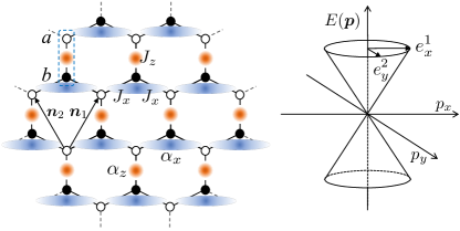
Fig. 1: (Left) The optical lattice configuration with fermionic and bosonic atoms. The unit cell of the honeycomb lattice (dashed box) comprises two fermionic modes $a$ and $b$. The fermionic atoms tunnel along the three different directions of the trivalence lattice with couplings $J_{x}$, $J_{y}(=J_{x})$, and $J_{z}$. The vectors ${\boldsymbol{n}}_{1}=(\sqrt{3}/2,3/2)$ and ${\boldsymbol{n}}_{2}=(-\sqrt{3}/2,3/2)$ transport between different unit cells. (Right) In the low energy limit the dispersion relation $E({\boldsymbol{p}})$ of the fermions is given by Dirac cones. Non-equal tunnelling couplings, $J_{x}$ and $J_{z}$, cause the Dirac cone to be deformed, with its geometry encoded in the dreibein components $e^{1}_{x}$ and $e^{2}_{y}$, effectively describing background gravity. Bosonic modes $\alpha_{x}$ and $\alpha_{z}$, describing Bose-Einstein condensates, are inserted that control the fermionic tunnelling couplings with their populations. Fluctuations of the condensates simulate fluctuations in $e^{1}_{x}$ and $e^{2}_{y}$, i.e. gravitational fluctuations.

III Optical lattice simulator

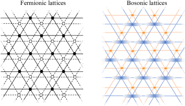
Fig. 2: The optical lattice configuration of Figure 1 is obtained by superposing two pairs of triangular lattices, a fermionic pair (Left) and a bosonic pair (Right). The pair of lattices that hosts fermionic modes $a$ and $b$ gives rise to the honeycomb lattice model when nearest neighbour tunnelling couplings are activated. The pair of bosonic lattice modes, $\alpha_{x}$ and $\alpha_{z}$, is positioned at the links of the honeycomb lattice. The $x$-confinement of the $\alpha_{x}$ modes is made weaker to overlap with both $J_{x}$ and $J_{y}$ links of the honeycomb lattice (see Figure 1). By activating interactions between the bosonic and fermionic atoms, $\Delta_{m}\alpha^{\dagger}_{m}\alpha_{m}a^{\dagger}_{\boldsymbol{i}}b_{\boldsymbol{k}}$, the population of the bosonic modes at site $m$ controls the fermionic tunnelling between sites ${\boldsymbol{i}}$ and ${\boldsymbol{k}}$, thus giving rise to the effective interaction between Dirac fields and fluctuating geometry.

We now design an optical lattice configuration that simulates the quantum gravity model given by (10) in its low energy limit. We first present a configuration that gives rise to Dirac fermions in a fixed background geometry encoded in the tunnelling couplings of the lattice [14]. Then we introduce link quantum variables $d_{m}$ $(m=x,z)$ that fluctuate this geometry. Consider a two-dimensional optical lattice with honeycomb configuration where fermionic atoms, $a$ and $b$, live at its vertices, as shown in Figure 1(Left). The fermions are subject to the tunnelling Hamiltonian

$$H_{\text{latt}}=\sum_{\boldsymbol{i}}\big{[}J_{x}(\boldsymbol{i})a_{\boldsymbol{i}}^{\dagger}b_{\boldsymbol{i}+\boldsymbol{n}_{1}}+J_{y}(\boldsymbol{i})a_{\boldsymbol{i}}^{\dagger}b_{\boldsymbol{i}+\boldsymbol{n}_{2}}+J_{z}(\boldsymbol{i})a_{\boldsymbol{i}}^{\dagger}b_{\boldsymbol{i}}\big{]}+\text{h.c.},$$ (14)

where ${\boldsymbol{i}}=(i_{x},i_{y})$ gives the position of unit cells on the lattice, the couplings of the first two terms are equal ($J_{x}=J_{y}$), and both $J_{x}$ and $J_{z}$ are in general position dependent. At half-filling, the low energy sector of the model is described by the Dirac Hamiltonian $H_{\text{latt}}\approx\int d^{2}x\;\psi^{\dagger}\;\tilde{h}({\boldsymbol{p}})\;\psi$ [14] with (see Appendix D for details)

$$\tilde{h}({\boldsymbol{p}}) =-\frac{\sqrt{3}i}{2}\sqrt{4J_{x}^{2}-J_{z}^{2}}\,\gamma^{0}\gamma^{1}\partial_{x}-\frac{3i}{2}J_{z}\gamma^{0}\gamma^{2}\partial_{y}$$ (15)

$$+\frac{\sqrt{3}i}{2}\partial_{x}\left(\sqrt{4J_{x}^{2}-J_{z}^{2}}\,\right)\gamma^{0}\gamma^{1}+\frac{3i}{2}\partial_{y}J_{z}\gamma^{0}\gamma^{2}.$$

The coefficients of $\gamma^{0}\gamma^{1}(-i\partial_{x})$ and $\gamma^{0}\gamma^{2}(-i\partial_{y})$ play the role of the diagonal space components of the dreibein, $e^{1}_{x}$ and $e^{2}_{y}$, respectively, as shown in Figure 1 (Right). To introduce quantum fluctuations in the $J$ couplings, and thus in the corresponding dreibeins, we insert bosonic modes $\alpha_{x}$ and $\alpha_{z}$ at the edges of the lattice, as shown in Figure 1 (Left). To realise this configuration of atomic boson-fermion mixture we need two pairs of triangular lattices, one fermionic and one bosonic, as shown in Figure 2. Triangular lattices can routinely be created in the laboratory for bosonic [55] and fermionic [56] atoms. Optical lattices with interacting mixtures of bosonic and fermionic atoms have been realised and their rich physics has been extensively investigated [57, 58, 59].

When the bosonic and fermionic lattices shown in Figure 2 are superposed, the bosonic modes $\alpha_{x}$ and $\alpha_{z}$ control the tunnelling of fermions from site $\boldsymbol{i}$ to site $\boldsymbol{k}$ in the $m(=x,z)$ direction, through the interaction $\Delta_{m}\alpha^{\dagger}_{m}\alpha_{m}a^{\dagger}_{\boldsymbol{i}}b_{\boldsymbol{k}}$ [15]. We take the $\alpha_{j}$ modes to correspond to a bosonic condensation with particle density $D_{m}$ and quantum fluctuations $d_{m}$, i.e.

$$\alpha_{m}(\boldsymbol{i})=D_{m}(\boldsymbol{i})+d_{m}(\boldsymbol{i}),$$ (16)

where $[d_{m}(\boldsymbol{i}),d_{m}^{\dagger}(\boldsymbol{j})]=\delta_{\boldsymbol{i}\boldsymbol{j}}$, for $m=x,z$. In the weak fluctuation limit $\langle d^{\dagger}_{m}d_{m}\rangle\ll D_{m}^{2}$, the interactions between bosons and fermions give rise to tunnelling couplings of the form $J_{m}=\Delta_{m}D_{m}(D_{m}+d_{m}^{\dagger}+d_{m})$. If we choose the optical lattice parameters as

$$D_{x}=\sqrt{2}D_{z}=-{l\over 4\pi G}\,,\qquad\Delta_{x}={\Delta_{z}\over 2}=\frac{32\pi^{2}G^{2}}{3l^{3}},$$ (17)

with the operator redefinition $q_{1}={2\sqrt{2}}d_{x}/3-d_{z}/3$ and $q_{2}=d_{z}$ that preserves bosonic commutation relations, we find that, to linear order in $G$, the optical lattice Hamiltonian (14) is mapped to the field theory one (11) (for details, see Appendices C and D). Constant tunnelling terms can be added in (14) to arbitrarily tune the values of the densities $D_{m}$.

The self-interaction terms (12) of the gravitational Hamiltonian can be obtained from the following purely bosonic interactions

$$\mathcal{H}_{\text{boson}}= \frac{1}{24\pi G}(\alpha_{z}^{\dagger}-\alpha_{z})\left(\sqrt{2}(\alpha_{x}^{\dagger}-\alpha_{x})-\frac{1}{2}(\alpha_{z}^{\dagger}-\alpha_{z})\right)$$ (18)

$$+\frac{8\pi G\mu^{2}}{3}\left(\alpha^{\dagger}_{z}\alpha_{z}+\alpha^{\dagger}_{x}\alpha_{x}\right)$$

$$-\frac{256\pi^{3}G^{3}\mu^{2}}{3l^{2}}\alpha^{\dagger}_{z}\alpha_{z}\left(\alpha^{\dagger}_{x}\alpha_{x}-\frac{1}{2}\alpha^{\dagger}_{z}\alpha_{z}\right),$$

restricted to the weak fluctuation regime of $\alpha_{m}$.

III.1 Realisation of interactions

The quantum simulation of Dirac fermions coupled to fluctuating gravity requires the realisation of (10) with the fermionic part coupled to the bosons given by (11) and the self-interactions of bosons (18). The first component is the realisation of the $(2+1)$-dimensional Dirac dispersion relation of the form (15). This has already been achieved in the laboratory with ultracold fermionic atoms by several experimental groups [60, 61, 62]. Of much interest is the possibility the optical lattices offer in running the couplings at will thus allowing the effective encoding of background geometry [14]. Introducing fluctuations in the background geometry can be achieved with optical lattices by coupling bosonic and fermionic species together, as shown in Figure 1(Left). This method is similar to the minimal coupling realisation with optical lattices [15], suitably adapted here to encode the coupling between Dirac fermions and dreibeins. It incorporates Bose-Einstein condensates with weak boson number fluctuations. When positioned at the links of the honeycomb lattice they couple with the tunnelling fermions producing the desired boson-fermion couplings dictated by (11). Note that the tunnelling couplings of fermions, $J_{x}$, $J_{y}$ and $J_{z}$, and the condensation particle densities $D_{m}$ can be routinely tuned and controlled in an experiment by controlling the laser intensity of the optical lattices and the frequency of the magnetic or optical trapping of the condensate, respectively.

Fig. 3: Realisation of the self-interacting terms of the gravitational bosonic modes $\alpha_{x}$ and $\alpha_{z}$. Tunnelling couplings of the form $J(\alpha_{x}^{\dagger}\alpha_{z}+\alpha_{z}^{\dagger}\alpha_{x})$ are produced by the overlap of the wavefunctions of the modes that sit in different wells. The tunnelling coupling $J$ is controlled by the barrier between the potential wells tuned by the laser intensity of the optical lattices. Feshbach resonances are produced by the elastic scattering collisions between $\alpha_{x}$ and $\alpha_{z}$ atoms with a rate that can be easily tuned by a magnetic field.

The final ingredient is the realisation of the gravitational self-interacting terms presented in (18). This Hamiltonian includes chemical potentials as well as tunnelling, pairing and interacting terms between the $\alpha_{m}$ bosonic atoms. Chemical potentials can be easily tuned with great accuracy by controlling the populations or the trapping potential of the cold atoms. Tunnelling terms between two different bosonic modes, such as $\alpha_{x}$ and $\alpha_{z}$, can be obtained by changing the potential barrier between the corresponding sites, as shown in Figure 3. These bosonic terms can be controlled independently from the fermionic atoms as they are created by independent optical lattices (see Appendix E for details). Pairing terms of the form $\alpha^{\dagger}_{z}\alpha^{\dagger}_{x}+\alpha_{z}\alpha_{x}$ can be activated by resonances to molecular bound states as it has been recently demonstrated with homonuclear ³⁹K-³⁹K or heteronuclear ⁴¹K-⁸⁷Rb mixtures [46, 47]. Population interactions of the form $\alpha^{\dagger}_{z}\alpha_{z}\alpha^{\dagger}_{x}\alpha_{x}$ can be accurately controlled by employing Feshbach resonances, e.g. between Rb atoms, as has already been demonstrated experimentally  [44, 45] (see Figure 3). Such resonances are very versatile as they can generate positive, negative or zero interactions, or change the collision rate by several orders of magnitude just by selecting appropriate atomic states and tuning appropriately the external magnetic field. Hence, it is plausible that the quantum gravity model coupled to Dirac fermions given in (10) can be experimentally realised with a mixture of bosonic and fermionic ultra-cold atoms in optical lattices.

IV Quantum signatures of gravity

The optical lattice system given by (14) and (18) in the low energy limit simulates Dirac fermions coupled to massive gravitons (10). The presence of simulated quantum effects of gravity can be witnessed by directly measuring the bosonic field or by measuring the effect it has on the fermionic field. The pure gravity Hamiltonian (12) describes simple tunnelling and pairing terms between bosonic modes 1 and 2. The signatures of these couplings can be directly measured in the quantum correlations $\langle d_{1}^{\dagger}d_{2}^{\dagger}\rangle$ and $\langle d_{1}^{\dagger}d_{2}\rangle$ of the corresponding Bose-Einstein condensates [63]. We can establish how faithfully the simulating Hamiltonian (18) reproduces the desired gravitational Hamiltonian (12) by determining the dependence of the correlations on the “gravitational” coupling $G$.

We present now how to identify the presence of a fluctuating gravitational field from the behaviour of the fermionic quantum correlations. In the absence of gravity, i.e. $G=0$, the interaction term of the Dirac field disappears giving rise to free fermions. If the fermions are coupled to a fluctuating gravitation field then interactions between them emerge. Hence, we can identify the presence of fluctuating geometry by identifying if the Dirac fermions are free or interacting. The distinction between the two can happen by testing the applicability of Wick’s theorem, i.e. testing the decomposition of four-point quantum correlations in terms of two-point correlations. Such two- and four-point correlation measurements are routinely realised in cold atom experiments. Hence, our scheme provides a direct quantum signature of gravity in terms of experimentally feasible components.

The partition function of the system at temperature $T$ is given by

$$Z=\int\mathcal{D}\,\xi\mathcal{\,}\mathcal{D}\pi\mathcal{\,}\mathcal{D}\psi\mathcal{D}\bar{\psi}\,\exp\left(-\frac{1}{k_{B}T}\int d^{2}x\;\mathcal{H}\right),$$ (19)

where $\mathcal{H}=\psi^{\dagger}\;h({\boldsymbol{p}})\;\psi+\mathcal{H}_{\text{gr}}$ and $k_{B}$ is the Boltzmann constant. To determine the behaviour of the fermions due to their interactions mediated by gravitational fluctuations we can integrate the bosonic part, i.e. $\xi$ and $\pi$, our from (19) and derive the effective fermionic Hamiltonian. Integrating out the momenta, $\pi^{i}_{a}$, leads to an irrelevant global factor in $Z$. We can subsequently integrate out the bosonic field $\xi^{a}_{i}$, which up to an overall constant yields

$$Z=\int\mathcal{D}\psi\mathcal{D}\bar{\psi}\exp\left(-\frac{1}{k_{B}T}\int d^{2}x\;\mathcal{H}_{\text{eff}}\right),$$ (20)

with the effective Hamiltonian

$$\mathcal{H}_{\text{eff}}=-i\bar{\psi}\gamma^{i}\partial_{i}\psi-\frac{4\pi G}{l^{2}\mu^{2}}\epsilon_{ab}\epsilon^{ij}{\cal J}_{i}^{a}{\cal J}_{j}^{b},$$ (21)

where ${\cal J}_{i}^{a}=\frac{i}{2l}\left(\bar{\psi}\gamma^{a}\partial_{i}\psi-\partial_{i}\bar{\psi}\gamma^{a}\psi\right)$ is the fermionic current. As a result the partition function of the system is Hubbard-like, effectively describing interacting fermions with a coupling proportional to the gravitational constant $G$. The presence of such attractive fermion interactions can be measured in optical lattices by monitoring its Hubbard-like behaviour [64]. It is interesting to note that similarity of the interaction term in (21) and the effective gravitational models considered in [2, 1].

An alternative manifestation of interactions (21) mediated by the gravitational field is on the fermionic correlations, which can be witnessed by testing the applicability of Wick’s theorem. In the absence of gravitational fluctuations, i.e. for Newton’s constant $G\to 0$ in (2) or for fluctuations $\xi_{i}^{a}\to 0$, the effective partition function corresponds to free fermions, as seen by (21). For this case, Wick’s theorem states that all four-point quantum correlators of the ground state can be exactly decomposed in terms of two-point correlators. Such four-point correlators of fermions can be expressed in terms of fermionic densities and two-point correlations and thus can be directly measured in cold atom experiments [42]. When the interactions induced by the gravitational field are present, i.e. for $G\neq 0$, Wick’s decomposition does not apply, leaving a difference that can be determined by measurements of fermionic correlations [49]. In the perturbative regime considered here this difference gives a measure of the coupling $G$ between the Dirac fermions and the gravitational field.

V Conclusions

Among the forces of nature gravity keeps its quantum aspects well hidden. This lack of experiential evidence hinders the theoretical understanding of quantum gravity and its unification with the rest of the fundamental forces within the Standard Model. Here we propose a way of simulating quantum signatures of massive gravity coupled to Dirac fermions in the laboratory. By building upon recent methods, developed for simulating scalar or gauge fields coupled to Dirac fermions, we are able to model Dirac fermions in the presence of fluctuating geometries, which is a unique characteristic of quantum gravity. This breakthrough was possible by encoding spacetime geometries intrinsically in the couplings of the system and then employing bosonic fields that fluctuate these couplings. The bosonic fields are appropriately designed in order to give rise to quantum a massive graviton akin to the magnetoroton emerging in fractional quantum Hall liquids. As our model provides a direct link between microscopic system components and properties of the effective massive gravity, it sheds light into the mechanism behind the emergence of quantum gravitons in strongly interacting systems.

Beyond providing an example where massive gravitons emerge in a condensed matter system, our model can be simulated with optical lattices. The components used in our proposal, such as the fermionic honeycomb lattice or the bosonic condensates, can be realised in the laboratory with current ultra-cold atom technology. Quantum signatures of the emerging geometry can be witnessed in the effective fermionic interactions mediated by their coupling to fluctuating geometry, which can be directly probed in optical lattice experiments.

Our work opens up a host of various applications. It is intriguing to consider the behaviour of various quantum gravity and cosmology theories in $1+1$, $2+1$ or $3+1$ dimensions with or without fermions. Several open questions exist about the quantum aspects of gravity, cosmology and the physics of black holes that can be addressed within the framework presented here. We envision that our proposal will initiate a new line of investigations where interacting models that simulate gravity can be realised in the laboratory and guide theoretical investigations towards the understanding of quantum aspects of gravity in nature.

Appendix A Spin connection

We consider a three-dimensional geometry whose metric tensor is defined by a set of dreibeins $e^{A}_{\mu}$

$$g_{\mu\nu}=\eta_{AB}e^{A}_{\mu}e^{B}_{\nu}.$$ (22)

where here $A=(0,a=1,2)$ denotes Lorentz indices, $\mu=(t,i=x,y)$ stand for manifold indices, and $\eta={\rm diag}(-,+,+)$ is the Minkowski metric. Parallel transport is defined by the spin connection $\omega^{A}_{\mu}$, which can be obtained from the vielbein postulate

$$\partial_{\mu}e^{A}_{\nu}-\Gamma^{\rho}_{\mu\nu}e^{A}_{\rho}+\epsilon^{A}_{\;BC}\omega^{B}_{\mu}e^{C}_{\nu}=0,$$ (23)

where $\Gamma^{\rho}_{\mu\nu}$ is the affine Christoffel connection and $\epsilon^{ABC}$ the Levi-Civita symbol ($\epsilon^{012}=1$). In this case, the gravitational fluctuations translate into fluctuations of the dreibein and the spin connection

$$e^{A}_{\mu}=\bar{e}^{A}_{\mu}+\frac{1}{8\pi G}\xi^{A}_{\mu}\,,\qquad\omega^{A}_{\mu}=\bar{\omega}^{A}_{\mu}+\frac{1}{8\pi G}v^{A}_{\mu}.$$ (24)

We restrict the analysis to flat backgrounds with constant dreibein and vanishing spin connection. Therefore we set

$$\bar{e}^{A}_{\mu}=constant\,,\qquad\bar{\omega}^{A}_{\mu}=0.$$ (25)

Furthermore, we consider torsionless geometries. In this case taking the antisymmetric part of (23) allows one to express $\omega^{A}_{\mu}$ in terms the dreibein and its derivatives. For the corresponding perturbations (24) one finds the relation

$$\epsilon^{\mu\nu\rho}\left(\partial_{\nu}\xi^{A}_{\rho}+\epsilon^{A}_{\;BC}\,\bar{e}^{B}_{\nu}v^{C}_{\rho}\right)=0,$$ (26)

which can be used to find the form of the spin connection perturbations $v^{A}_{\mu}$

$$v^{A}_{\mu}=M^{AB}_{\mu\nu}\epsilon^{\nu\alpha\beta}\partial_{\alpha}\xi_{B\beta}\,,\quad M^{AB}_{\mu\nu}\equiv\frac{1}{\bar{e}}\left(\frac{1}{2}\bar{e}^{A}_{\mu}\bar{e}^{B}_{\nu}-\bar{e}^{A}_{\nu}\bar{e}^{B}_{\mu}\right),$$ (27)

where $\bar{e}={\rm det}(\bar{e}^{A}_{\mu})$. When restricted to metrics of the form (1), which means

$$\bar{e}^{A}_{\mu}=\begin{pmatrix}1&0\\ 0&\bar{e}^{a}_{i}\end{pmatrix}\,,\qquad\xi^{a}_{\mu}=\begin{pmatrix}0&0\\ 0&\xi^{a}_{i}\end{pmatrix},$$ (28)

the components of the spin connection reduce to

$$v^{0}_{t}=-\frac{4\pi G}{\bar{e}}\epsilon^{ij}\bar{e}^{a}_{i}\dot{\xi}_{aj}\,,\qquad v^{0}_{i}=-\frac{8\pi G}{\bar{e}\,}\epsilon^{jk}\bar{e}^{a}_{i}\partial_{j}\xi_{ak}\,,$$ (29)

$$v^{a}_{t}=0\,,\qquad\qquad v^{a}_{i}=8\pi GM^{ab}_{ij}\epsilon^{jk}\dot{\xi}_{bk}\,.$$

Appendix B Gravity action

In order to describe gravitational fluctuations, we start with the Palatini action for $e^{A}_{\mu}$ and $\omega^{A}_{\mu}$

$$S_{\text{gr}}=\frac{1}{8\pi G}\int d^{3}x\,\epsilon^{\mu\nu\rho}e^{A}_{\mu}\left(\partial_{\nu}\omega_{A\rho}+\frac{1}{2}\epsilon_{ABC}\;\omega^{B}_{\nu}\omega^{C}_{\nu}\right).$$ (30)

Using (24), the action can be expanded in powers of the (2+1)-dimensional reduced Planck mass $1/8\pi G$ as

$$S_{\text{gr}}[\xi]=\frac{1}{8\pi G}S_{\text{gr}}^{(0)}+S_{\text{gr}}^{(1)}+8\pi G\,S_{\text{gr}}^{(2)}.$$ (31)

Defining the background curvature and torsion,

$$\bar{R}^{A}_{\mu\nu}=\partial_{[\mu}\bar{\omega}^{A}_{\nu]}+\frac{1}{2}\epsilon^{A}_{BC}\bar{\omega}^{B}_{[\mu}\bar{\omega}^{C}_{\nu]}=0,$$ (32)

$$\bar{T}^{A}_{\mu\nu}=\partial_{[\mu}\bar{e}^{A}_{\nu]}+\epsilon^{A}_{BC}\bar{\omega}^{B}_{[\mu}\bar{e}^{C}_{\nu]}=0,$$

the different terms in the action (31) can be written as

$$S_{\text{gr}}^{(0)} =\frac{1}{2}\int d^{3}x\,\epsilon^{\mu\nu\rho}\bar{e}^{A}_{\mu}\bar{R}_{A\nu\rho},$$ (33)

$$S_{\text{gr}}^{(1)} =\frac{1}{2}\int d^{3}x\,\epsilon^{\mu\nu\rho}\left(\xi^{A}_{\mu}\bar{R}_{A\nu\rho},+\bar{v}^{A}_{\mu}\bar{T}_{A\nu\rho}\right),$$

$$S_{\text{gr}}^{(2)} =\int d^{3}x\,\epsilon^{\mu\nu\rho}\left(\xi^{A}_{\mu}\bar{D}_{\nu}v_{A\rho}+\frac{1}{2}\epsilon_{ABC}\;\bar{e}^{A}_{\mu}v^{B}_{\nu}v^{C}_{\rho}\right).$$

Considering a flat torsionless background implies that $\bar{R}^{A}_{\mu\nu}=0=\bar{T}^{A}_{\mu\nu}$. Replacing (27) in (33) and using tensor notation then yields

$$S_{\text{gr}}[\xi]=-4\pi G\int d^{3}xM^{AB}_{\mu\nu}\epsilon^{\mu\alpha\beta}\epsilon^{\nu\gamma\delta}\partial_{\alpha}\xi_{A\beta}\partial_{\gamma}\xi_{B\delta}.$$ (34)

One can check that the action (34) boils down to the massless Fierz-Pauli action for $h_{\mu\nu}=\bar{e}_{A\mu}\xi^{A}_{\nu}+\bar{e}_{A\nu}\xi^{A}_{\mu}$.

We are interesting in adding a mass $\mu$ to the geometry fluctuations $\xi^{A}_{\mu}$. We do so by means of the Fierz-Pauli mass term

$$4\pi G\mu^{2}\epsilon^{\mu\nu\rho}\epsilon_{ABC}\,\bar{e}^{A}_{\mu}\xi^{B}_{\nu}\xi^{C}_{\rho}\,.$$ (35)

Thus, implementing (28) and (29) in (34) and adding the term (35) restricted to those conditions, we find the following effective massive gravitational action

$$S_{\text{gr}}[\xi]=-4\pi G\int d^{3}x\epsilon^{ij}\epsilon_{ab}\bigg{(}\dot{\xi}^{a}_{i}\dot{\xi}^{b}_{j}-\mu^{2}\xi^{a}_{i}\xi^{b}_{j}\bigg{)}.$$ (36)

where we have defined $\epsilon^{ij}\equiv\epsilon^{0ij}$.

Appendix C Field theory Hamiltonian

The Hamiltonian density associated to the Lagrangian in (4) is obtained after a straightforward Legendre transformation.

$$\mathcal{H}=\Pi^{\dagger}\dot{\psi}+\dot{\psi}\Pi+\pi_{a}^{i}\dot{\xi}^{a}_{i}-\mathcal{L},$$ (37)

where the canonical momenta read

$$\Pi^{\dagger}=\frac{\partial\mathcal{L}}{\partial\dot{\psi}}=i\psi^{\dagger}\,,\qquad\Pi=\frac{\partial\mathcal{L}}{\partial\dot{\psi}^{\dagger}}=0\,,$$ (38)

$$\pi_{a}^{i}=\frac{\partial\mathcal{L}}{\partial\dot{\xi}^{a}_{i}}=-8\pi G\epsilon^{ij}\epsilon_{ab}\dot{\xi}^{b}_{j},$$

and satisfy the Poisson brackets

$$\left\{\psi_{\alpha}(x),\Pi^{\dagger}_{\beta}(y)\right\}=\left\{\psi^{\dagger}_{\alpha}(x),\Pi_{\beta}(y)\right\}=-\delta_{\alpha\beta}\delta^{(2)}(x-y),$$ (39)

$$\left\{\xi^{a}_{i}(x),\pi_{b}^{j}(y)\right\}=\delta^{a}_{b}\delta^{j}_{i}\delta^{(2)}(x-y).$$

The Hamiltonian reduces to

$$H=\int d^{2}x\;\mathcal{H}=\int d^{2}x\;\left[\psi^{\dagger}\;h(\boldsymbol{p})\;\psi+\mathcal{H}_{\text{gr}}\right],$$ (40)

with the single particle hamiltonian $h(\boldsymbol{p})$

$$h(\boldsymbol{p})=\frac{\gamma^{0}}{l}\left(\delta^{i}_{a}\gamma^{a}-\frac{8\pi G}{l}\xi^{i}_{a}\gamma^{a}\right)(-i\partial_{i})+\frac{4i\pi G}{l^{2}}\partial_{i}\xi^{i}_{a}\gamma^{0}\gamma^{a},$$ (41)

and the gravitational Hamiltonian $\mathcal{H}_{\text{gr}}$ given by

$$\mathcal{H}_{\text{gr}}=-\frac{1}{16\pi G}\epsilon_{ij}\epsilon^{ab}\pi_{a}^{i}\pi_{b}^{j}-{4\pi G\mu^{2}}\epsilon^{ij}\epsilon_{ab}\xi^{a}_{i}\xi^{b}_{j}.$$ (42)

Since our analysis considers geometry fluctuations $\xi^{a}_{i}$ that are diagonal, we define quantum operators of the form

$$\xi^{a}_{i}=\begin{pmatrix}\xi^{1}_{x}&0\\ 0&\xi^{2}_{y}\end{pmatrix}\,,\qquad\begin{aligned} &\xi^{1}_{x}=\frac{1}{\sqrt{2}}(q_{1}^{\dagger}+q_{1})\,,\\ &\xi^{2}_{y}=\frac{1}{\sqrt{2}}(q_{2}^{\dagger}+q_{2}),\end{aligned}$$ (43)

where the operators $q_{a}$ and $q^{\dagger}_{a}$ $(a=1,2)$ satisfy the commutation relations

$$[q_{a}(x),q_{b}^{\dagger}(y)]=\delta_{ab}\delta^{(2)}(x-y),$$ (44)

$$[q_{a}(x),q_{b}(y)]=0=[q_{a}^{\dagger}(x),q_{b}^{\dagger}(y)].$$

Thus, the canonical Poisson brackets (39) are promoted commutators $\{\;,\;\}\rightarrow-i[\;\,\;]$, which then fixes the form of the momenta $\xi_{a}^{i}$ to be

$$\pi_{a}^{i}=\begin{pmatrix}\pi_{1}^{x}&0\\ 0&\pi_{2}^{y}\end{pmatrix}\,,\qquad\begin{aligned} &\pi_{1}^{x}=-\frac{i}{\sqrt{2}}(q_{1}^{\dagger}-q_{1})\,,\\ &\pi_{2}^{y}=-\frac{i}{\sqrt{2}}(q_{2}^{\dagger}-q_{2}).\end{aligned}$$ (45)

The flat background spatial metric is taken as $g_{ij}=l^{2}\delta_{ij}$ with $l$ an arbitrary constant, which implies

$$\bar{e}^{a}_{i}=l\delta^{a}_{i}\,,\qquad\bar{e}^{i}_{a}=\frac{1}{l}\delta^{i}_{a}\,,$$ (46)

and thus the gamma matrices on this background geometry reduce to

$$\gamma^{t}=\gamma^{0}\,,\quad\gamma^{i}=\frac{1}{l}\delta^{i}_{a}\gamma^{a}.$$ (47)

From this expressions we see that the single particle Hamitlonian (41) can be written as

$$h(\boldsymbol{p}) =\left(\frac{1}{l}-\frac{4\sqrt{2}\pi G}{l^{2}}(q_{1}^{\dagger}+q_{1})\right)\gamma^{0}\gamma^{1}(-i\partial_{x})$$ (48)

$$+\left(\frac{1}{l}-\frac{4\sqrt{2}\pi G}{l^{2}}(q_{2}^{\dagger}+q_{2})\right)\gamma^{0}\gamma^{2}(-i\partial_{y})$$

$$+\frac{2\sqrt{2}i\pi G}{l^{2}}\left(\partial_{x}(q_{1}^{\dagger}+q_{1})\gamma^{0}\gamma^{1}+\partial_{y}(q_{2}^{\dagger}+q_{2})\gamma^{0}\gamma^{2}\right),$$

whereas the gravitational Hamiltonian (42) takes the form

$$\mathcal{H}_{\rm gr}=\frac{1}{16\pi G}(q_{1}^{\dagger}-q_{1})(q_{2}^{\dagger}-q_{2})-4\pi G\mu^{2}(q_{1}^{\dagger}+q_{1})(q_{2}^{\dagger}+q_{2}).$$ (49)

In the following, we show how to translate (40) into an optical lattice Hamiltonian.

Appendix D Optical Lattice Hamiltonian

We start considering an optical lattice with unequal tunnelling couplings

$$H_{\rm latt}=\sum_{\boldsymbol{i}}\left(J_{x}a_{\boldsymbol{i}}^{\dagger}b_{\boldsymbol{i}+\boldsymbol{n}_{1}}+J_{y}a_{\boldsymbol{i}}^{\dagger}b_{\boldsymbol{i}+\boldsymbol{n}_{2}}+J_{z}a_{\boldsymbol{i}}^{\dagger}b_{\boldsymbol{i}}\right)+{\rm h.c.},$$ (50)

where $\boldsymbol{i}=(i_{x},i_{y})$ denotes the position of the unit cells (see Figure 1). Expanding the operators in Fourier modes and defining

$$\psi_{\boldsymbol{k}}=\begin{pmatrix}a_{\boldsymbol{k}}\\ b_{\boldsymbol{k}}\end{pmatrix},\quad\tilde{h}({\boldsymbol{k}})=\begin{pmatrix}0&f(\boldsymbol{k})\\ f^{*}(\boldsymbol{k})&0\end{pmatrix},$$ (51)

where $f(\boldsymbol{k})=J_{x}e^{-i\boldsymbol{k}\cdot\boldsymbol{n}_{1}}+J_{y}e^{-i\boldsymbol{k}\cdot\boldsymbol{n}_{2}}+J_{z}$, we find

$$H_{\rm latt}=\sum_{\boldsymbol{k}}\psi^{\dagger}_{\boldsymbol{k}}\tilde{h}(\boldsymbol{k})\psi_{\boldsymbol{k}}.$$ (52)

We consider the special case $J_{x}=J_{y}$. The Fermi points, $\boldsymbol{P}_{\pm}$, are defined by

$$f(\boldsymbol{P}_{\pm})=0\Rightarrow\boldsymbol{P}_{\pm}=\pm\begin{pmatrix}\frac{2}{\sqrt{3}}\arccos(-J_{z}/J_{x})\\ 0\end{pmatrix}.$$ (53)

Now, we expand $f(\boldsymbol{k})$ around the Fermi points

$$f(\boldsymbol{P}_{\pm}+\boldsymbol{p})=\boldsymbol{p}\cdot\nabla f(\boldsymbol{P}_{\pm})=A_{\pm}p_{x}+B_{\pm}p_{y},$$ (54)

where we have defined

$$A_{\pm}=\mp\frac{\sqrt{3}}{2}\sqrt{4J_{x}^{2}-J_{z}^{2}},\quad B_{\pm}=-\frac{3}{2}J_{z}.$$ (55)

Expanding the Hamiltonian $H_{\rm latt}$ around the Fermi point yields

$$H_{\rm latt} =\sum_{\boldsymbol{p}}\begin{pmatrix}a^{\dagger}_{+}\;\;b^{\dagger}_{+}\end{pmatrix}(A_{+}\sigma^{1}p_{x}-B_{+}\sigma^{2}p_{y})\begin{pmatrix}a_{+}\\ b_{+}\end{pmatrix}$$ (56)

$$+\sum_{\boldsymbol{p}}\begin{pmatrix}a^{\dagger}_{-}\;\;b^{\dagger}_{-}\end{pmatrix}(A_{-}\sigma^{1}p_{x}-B_{-}\sigma^{2}p_{y})\begin{pmatrix}a_{-}\\ b_{-}\end{pmatrix}.$$

Defining the four spinor and the gamma matrices

$$\psi_{\boldsymbol{p}}=\begin{pmatrix}a_{+}\\ b_{+}\\ b_{-}\\ a_{-}\end{pmatrix},\quad\gamma^{0}=\begin{pmatrix}0&-\boldsymbol{1}\\ \boldsymbol{1}&0\end{pmatrix},\quad\gamma^{i}=\begin{pmatrix}0&\sigma^{i}\\ \sigma^{i}&0\end{pmatrix},$$ (57)

with $\sigma^{i}=(\sigma^{1},\sigma^{2})$ Pauli matrices. Then we find $H_{\text{latt}}=\int d^{2}x\;\psi^{\dagger}\;\tilde{h}({\boldsymbol{p}})\;\psi$ with the single particle Hamiltonian

$$\tilde{h}(\boldsymbol{p})=\frac{\sqrt{3}}{2}\sqrt{4J_{x}^{2}-J_{z}^{2}}\,\gamma^{0}\gamma^{1}p_{x}+\frac{3}{2}J_{z}\gamma^{0}\gamma^{2}p_{y}.$$ (58)

where, for convenience, we have flipped the orientation of the $y$ axis, i.e. $p_{y}\shortrightarrow-p_{y}$. In order to ensure hermiticity of the full Hamiltonian, the momentum operator is defined as $p_{i}=-i(\overrightarrow{\partial}_{i}-\overleftarrow{\partial}_{i})/2$. Thus we find

$$\tilde{h}(\boldsymbol{p}) =\frac{\sqrt{3}}{2}\sqrt{4J_{x}^{2}-J_{z}^{2}}\,\gamma^{0}\gamma^{1}(-i\partial_{x})+\frac{3}{2}J_{z}\gamma^{0}\gamma^{2}(-i\partial_{y})$$ (59)

$$+\frac{\sqrt{3}i}{2}\partial_{x}\left(\sqrt{4J_{x}^{2}-J_{z}^{2}}\,\right)\gamma^{0}\gamma^{1}+\frac{3i}{2}\partial_{y}J_{z}\gamma^{0}\gamma^{2}.$$

We can now generalise this Hamiltonian by considering the couplings $J_{x}$ and $J_{z}$ as position dependent, varying slowly compared to the lattice spacing. Next, we add a bosonic self-interacting Hamiltonian $\mathcal{H}_{\text{boson}}$,

$$\mathcal{H}_{\text{boson}} =\frac{1}{24\pi G}(\alpha_{z}^{\dagger}-\alpha_{z})\left(\sqrt{2}(\alpha_{x}^{\dagger}-\alpha_{x})-\frac{1}{2}(\alpha_{z}^{\dagger}-\alpha_{z})\right)$$ (60)

$$+\frac{8\pi G\mu^{2}}{3}\left(\alpha^{\dagger}_{z}\alpha_{z}+\alpha^{\dagger}_{x}\alpha_{x}\right)$$

$$-\frac{256\pi^{3}G^{3}\mu^{2}}{3l^{2}}\alpha^{\dagger}_{z}\alpha_{z}\left(\alpha^{\dagger}_{x}\alpha_{x}-\frac{1}{2}\alpha^{\dagger}_{z}\alpha_{z}\right),$$

where $\alpha_{x}$ and $\alpha_{z}$ are bosonic modes at the edges of the lattice that control the tunneling of fermions in the $x$ and in the $z$ direction, respectively (see Figure 2). The optical lattice Hamiltonian that we will consider is then

$$H_{\rm latt}=\int d^{2}x \bigg{[}\psi^{\dagger}\;\tilde{h}(\boldsymbol{p})\;\psi+\mathcal{H}_{\text{boson}}\bigg{]}.$$ (61)

In order to show that (61) can be mapped to (40), first we consider the following form of the couplings

$$J_{m}=\Delta_{m}D_{m}\left(D_{m}+d_{m}^{\dagger}+d_{m}\right)\,,\quad m=x,z.$$ (62)

where the operators $d_{m}$ satisfy the commutation relations

$$[d_{m}(x),d_{n}^{\dagger}(y)]=\delta_{mn}\delta^{(2)}(x-y),$$ (63)

$$[d_{m}(x),d_{n}(y)]=0=[d_{m}^{\dagger}(x),d_{n}^{\dagger}(y)],$$

Note that this is a continuum version of the commutation relations given below Eq. (16). By considering

$$D_{x}=-{l\over 4\pi G}\,,\qquad\Delta_{x}=\frac{32\pi^{2}G^{2}}{3l^{3}},$$ (64)

$$D_{z}=-{\sqrt{2}l\over 8\pi G}\,,\qquad\Delta_{z}=\frac{64\pi^{2}G^{2}}{3l^{3}},$$

one finds that the different terms in $\tilde{h}(\boldsymbol{p})$ given in (59) can be written in the form

$$\frac{3}{2}J_{z} =\frac{1}{l}-\frac{4\sqrt{2}\pi G}{l^{2}}\left(d_{z}^{\dagger}+d_{z}\right),$$ (65)

$$\frac{\sqrt{3}}{2}\sqrt{4J_{x}^{2}-J_{z}^{2}} \approx\frac{1}{l}-\frac{16\pi G}{3l^{2}}\left(d_{x}^{\dagger}+d_{x}\right)$$

$$\hskip 22.76228pt+\frac{4\sqrt{2}\pi G}{3l^{2}}\left(d_{z}^{\dagger}+d_{z}\right),$$

where in the last equality we have used the approximation

$$\left|\left\langle d^{\dagger}_{m}+d_{m}\right\rangle\right|\ll\left|D_{m}\right|,$$ (66)

valid for bosonic states in the weak fluctuation regime. Finally, we consider the operator redefinition

$$q_{1}=\frac{2\sqrt{2}}{3}d_{x}-\frac{1}{3}d_{z}\,,\qquad q_{2}=d_{z},$$ (67)

which satisfy the canonical commutation relations given in (44). This transformation maps the single particle Hamiltonian $\tilde{h}(\boldsymbol{p})$, given (59), into the corresponding Hamiltonian $h(\boldsymbol{p})$ describing fermions coupled to dreibein fluctuations given in (48).

Now we turn our attention to the bosonic Hamiltonian (60), where the operators $\alpha_{m}$ are defined as

$$\alpha_{m}=D_{m}+d_{m}.$$ (68)

In this case we reverse the procedure and show that, up to an irrelevant additive constant, the gravitational Hamiltonian $\mathcal{H}_{\rm gr}$ given in (49) can be mapped to (60). This can be directly shown by noticing that

$$(d^{\dagger}_{m}-d_{m})(d^{\dagger}_{n}-d_{n}) =(\alpha^{\dagger}_{m}-\alpha_{m})(\alpha^{\dagger}_{n}-\alpha_{n}),$$ (69)

$$(d^{\dagger}_{m}+d_{m})(d^{\dagger}_{m}+d_{m}) \approx\frac{\alpha^{\dagger}_{m}\alpha_{m}\alpha^{\dagger}_{n}\alpha_{n}}{D_{m}D_{n}}-\frac{D_{m}}{D_{m}}\alpha^{\dagger}_{n}\alpha_{n}$$

$$-\frac{D_{n}}{D_{m}}\alpha^{\dagger}_{m}\alpha_{m}+D_{m}D_{n},$$

and using (64) and (67). Note that in the last relation we have used $\alpha^{\dagger}_{m}\alpha_{m}\approx D_{m}^{2}+D_{m}(d_{m}^{\dagger}+d_{m})$, which holds in the approximation (66).

Appendix E Optical lattice realisation of the gravitational Hamiltonan

In order to realise the bosonic Hamiltonian (18), we consider the Hamiltonian for bosonic atoms, described by a bosonic mode $\Phi({\bf x})$, in an optical lattice potential $V_{0}$ and a slowly varying external trapping potential $V_{T}$:

$$H= \int d^{3}x\,\,\Phi^{\dagger}({\bf x})\left[-\frac{\nabla^{2}}{2m}+V_{0}({\bf x})+V_{T}({\bf x})\right]\Phi({\bf x})$$ (70)

$$+\frac{2\pi a_{s}^{2}}{m}\int d^{3}x\,\,\Phi^{\dagger}({\bf x})\Phi^{\dagger}({\bf x})\Phi({\bf x})\Phi({\bf x})$$

where $a_{s}$ is the $s$-wave scattering length and $m$ is the mass of the atoms [65]. For single atoms the energy eigenstates are Bloch wave functions and an appropriate superposition of Bloch states yields a set of Wannier functions which are well localized on the individual lattice sites. Expanding the field operator in the Wannier basis $w({\bf x})$ in the following way,

$$\Phi({\bf x})=\sum_{i}\alpha_{i}\phi_{i}({\bf x}),\quad\phi_{i}({\bf x})=w({\bf x}-{\bf x}_{i}),\quad[\alpha_{i},\alpha_{j}^{\dagger}]=\delta_{ij}$$ (71)

one finds the Bose-Hubbard Hamiltonian

$$H=-\sum_{<ij>}t_{ij}\;\alpha_{i}^{\dagger}\alpha_{j}+\sum_{<ijkl>}U_{ijkl}\;\alpha_{i}^{\dagger}\alpha_{j}^{\dagger}\alpha_{k}\alpha_{l},$$ (72)

where $<\!\!\cdots\!\!>$ denotes summation only over nearest neighbours. In (72) we have defined the overlap integrals

$$t_{ij} =\int d^{3}x\,\phi^{*}_{i}({\bf x})\left(-\frac{\nabla^{2}}{2m}+V_{0}({\bf x})+V_{T}({\bf x})\right)\phi_{j}({\bf x})$$ (73)

$$U_{ijkl} =\frac{4\pi a_{s}^{2}}{m}\int d^{3}x\,\phi^{*}_{i}({\bf x})\,\phi^{*}_{j}({\bf x})\,\phi_{k}({\bf x})\,\phi_{l}({\bf x}),$$

where $t_{ij}$ represents the tunnelling couplings (or the hopping matrix elements), whereas $U_{ijkl}$ stands for the strength of the on-site repulsion of two atoms. We arrange the modes to be defined on a diamond lattice with indices $i=(\boldsymbol{i},m)$, $j=(\boldsymbol{j},n)$, etc, as shown in Figure 1. For particular values of $t_{ij}$ and $U_{ijkl}$, e.g. by changing the laser intensity or employing Feshbach resonances that control the scattering length, it is possible to tune appropriately the couplings and reproduce the gravitational Hamiltonian (18).

References

- Volovik [2021] G. E. Volovik. Gravity from symmetry breaking phase transition. 11 2021. doi: 10.1007/s10909-022-02694-z.
- Diakonov [2011] Dmitri Diakonov. Towards lattice-regularized Quantum Gravity. 9 2011.
- Girvin et al. [1985] S. M. Girvin, A. H. MacDonald, and P. M. Platzman. Collective-excitation gap in the fractional quantum hall effect. Phys. Rev. Lett., 54:581–583, Feb 1985. doi: 10.1103/PhysRevLett.54.581.
- Girvin et al. [1986] S. M. Girvin, A. H. MacDonald, and P. M. Platzman. Magneto-roton theory of collective excitations in the fractional quantum hall effect. Phys. Rev. B, 33:2481–2494, Feb 1986. doi: 10.1103/PhysRevB.33.2481.
- Golkar et al. [2016] Siavash Golkar, Dung Xuan Nguyen, Matthew M. Roberts, and Dam Thanh Son. Higher-spin theory of the magnetorotons. Phys. Rev. Lett., 117:216403, Nov 2016. doi: 10.1103/PhysRevLett.117.216403.
- Gromov and Son [2017] Andrey Gromov and Dam Thanh Son. Bimetric theory of fractional quantum hall states. Phys. Rev. X, 7:041032, Nov 2017. doi: 10.1103/PhysRevX.7.041032.
- Bergshoeff et al. [2018] Eric A. Bergshoeff, Jan Rosseel, and Paul K. Townsend. Gravity and the spin-2 planar schrödinger equation. Phys. Rev. Lett., 120:141601, Apr 2018. doi: 10.1103/PhysRevLett.120.141601.
- Pinczuk et al. [1993] A. Pinczuk, B. S. Dennis, L. N. Pfeiffer, and K. West. Observation of collective excitations in the fractional quantum hall effect. Phys. Rev. Lett., 70:3983–3986, Jun 1993. doi: 10.1103/PhysRevLett.70.3983.
- Kang et al. [2000] Moonsoo Kang, A. Pinczuk, B. S. Dennis, M. A. Eriksson, L. N. Pfeiffer, and K. W. West. Inelastic light scattering by gap excitations of fractional quantum hall states at . Phys. Rev. Lett., 84:546–549, Jan 2000. doi: 10.1103/PhysRevLett.84.546.
- Zhou et al. [2021] Zhao-Yu Zhou, Guo-Xian Su, Jad C Halimeh, Robert Ott, Hui Sun, Philipp Hauke, Bing Yang, Zhen-Sheng Yuan, Jürgen Berges, and Jian-Wei Pan. Thermalization dynamics of a gauge theory on a quantum simulator. arXiv preprint arXiv:2107.13563, 2021.
- Iorio et al. [2018] A. Iorio, P. Pais, I. A. Elmashad, A. F. Ali, Mir Faizal, and L. I. Abou-Salem. Generalized Dirac structure beyond the linear regime in graphene. Int. J. Mod. Phys. D, 27(08):1850080, 2018. doi: 10.1142/S0218271818500803.
- Ciappina et al. [2020] Marcelo F. Ciappina, Alfredo Iorio, Pablo Pais, and Adamantia Zampeli. Torsion in quantum field theory through time-loops on dirac materials. Phys. Rev. D, 101:036021, Feb 2020. doi: 10.1103/PhysRevD.101.036021.
- Boada et al. [2011] Octavi Boada, Alessio Celi, José I Latorre, and Maciej Lewenstein. Dirac equation for cold atoms in artificial curved spacetimes. New Journal of Physics, 13(3):035002, 2011.
- Farjami et al. [2020] Ashk Farjami, Matthew D. Horner, Chris N. Self, Zlatko Papić, and Jiannis K. Pachos. Geometric description of the kitaev honeycomb lattice model. Phys. Rev. B, 101:245116, Jun 2020. doi: 10.1103/PhysRevB.101.245116.
- Cirac et al. [2010] J. Ignacio Cirac, Paolo Maraner, and Jiannis K. Pachos. Cold atom simulation of interacting relativistic quantum field theories. Phys. Rev. Lett., 105:190403, Nov 2010. doi: 10.1103/PhysRevLett.105.190403.
- Achucarro and Townsend [1986] A. Achucarro and P. K. Townsend. A Chern-Simons Action for Three-Dimensional anti-De Sitter Supergravity Theories. Phys. Lett. B, 180:89, 1986. doi: 10.1016/0370-2693(86)90140-1.
- Witten [1988] Edward Witten. (2+1)-Dimensional Gravity as an Exactly Soluble System. Nucl. Phys. B, 311:46, 1988. doi: 10.1016/0550-3213(88)90143-5.
- Brown and Henneaux [1986] J. David Brown and M. Henneaux. Central Charges in the Canonical Realization of Asymptotic Symmetries: An Example from Three-Dimensional Gravity. Commun. Math. Phys., 104:207–226, 1986. doi: 10.1007/BF01211590.
- Coussaert et al. [1995] Oliver Coussaert, Marc Henneaux, and Peter van Driel. The Asymptotic dynamics of three-dimensional Einstein gravity with a negative cosmological constant. Class. Quant. Grav., 12:2961–2966, 1995. doi: 10.1088/0264-9381/12/12/012.
- Strominger [1998] Andrew Strominger. Black hole entropy from near horizon microstates. JHEP, 02:009, 1998. doi: 10.1088/1126-6708/1998/02/009.
- Barnich and Compere [2007] Glenn Barnich and Geoffrey Compere. Classical central extension for asymptotic symmetries at null infinity in three spacetime dimensions. Class. Quant. Grav., 24:F15–F23, 2007. doi: 10.1088/0264-9381/24/5/F01.
- Babichev et al. [2016] Eugeny Babichev, Luca Marzola, Martti Raidal, Angnis Schmidt-May, Federico Urban, Hardi Veermäe, and Mikael von Strauss. Heavy spin-2 Dark Matter. JCAP, 09:016, 2016. doi: 10.1088/1475-7516/2016/09/016.
- de Rham et al. [2011] Claudia de Rham, Gregory Gabadadze, and Andrew J. Tolley. Resummation of massive gravity. Phys. Rev. Lett., 106:231101, Jun 2011. doi: 10.1103/PhysRevLett.106.231101.
- Deser et al. [1982] Stanley Deser, R. Jackiw, and S. Templeton. Three-Dimensional Massive Gauge Theories. Phys. Rev. Lett., 48:975–978, 1982. doi: 10.1103/PhysRevLett.48.975.
- Bergshoeff et al. [2009a] Eric A. Bergshoeff, Olaf Hohm, and Paul K. Townsend. Massive Gravity in Three Dimensions. Phys. Rev. Lett., 102:201301, 2009a. doi: 10.1103/PhysRevLett.102.201301.
- Bergshoeff et al. [2013] Eric A. Bergshoeff, Sjoerd de Haan, Olaf Hohm, Wout Merbis, and Paul K. Townsend. Zwei-Dreibein Gravity: A Two-Frame-Field Model of 3D Massive Gravity. Phys. Rev. Lett., 111(11):111102, 2013. doi: 10.1103/PhysRevLett.111.111102. [Erratum: Phys.Rev.Lett. 111, 259902 (2013)].
- Schreiber et al. [2015] Michael Schreiber, Sean S Hodgman, Pranjal Bordia, Henrik P Lüschen, Mark H Fischer, Ronen Vosk, Ehud Altman, Ulrich Schneider, and Immanuel Bloch. Observation of many-body localization of interacting fermions in a quasirandom optical lattice. Science, 349(6250):842–845, 2015.
- Kondov et al. [2015] S. S. Kondov, W. R. McGehee, W. Xu, and B. DeMarco. Disorder-induced localization in a strongly correlated atomic hubbard gas. Phys. Rev. Lett., 114:083002, Feb 2015. doi: 10.1103/PhysRevLett.114.083002.
- White et al. [2009] M. White, M. Pasienski, D. McKay, S. Q. Zhou, D. Ceperley, and B. DeMarco. Strongly interacting bosons in a disordered optical lattice. Phys. Rev. Lett., 102:055301, Feb 2009. doi: 10.1103/PhysRevLett.102.055301.
- Choi et al. [2016] Jae-yoon Choi, Sebastian Hild, Johannes Zeiher, Peter Schauß, Antonio Rubio-Abadal, Tarik Yefsah, Vedika Khemani, David A Huse, Immanuel Bloch, and Christian Gross. Exploring the many-body localization transition in two dimensions. Science, 352(6293):1547–1552, 2016.
- [31] Karen Wintersperger, Christoph Braun, F. Nur Ünal, André Eckardt, Marco Di Liberto, Nathan Goldman, Immanuel Bloch, and Monika Aidelsburger. Realization of an anomalous floquet topological system with ultracold atoms. Nature Physics, (10):1058–1063. doi: 10.1038/s41567-020-0949-y.
- Scherg et al. [2021] Sebastian Scherg, Thomas Kohlert, Pablo Sala, Frank Pollmann, Bharath Hebbe Madhusudhana, Immanuel Bloch, and Monika Aidelsburger. Observing non-ergodicity due to kinetic constraints in tilted fermi-hubbard chains. Nature Communications, 12(1):1–8, 2021.
- Schweizer et al. [2019] Christian Schweizer, Fabian Grusdt, Moritz Berngruber, Luca Barbiero, Eugene Demler, Nathan Goldman, Immanuel Bloch, and Monika Aidelsburger. Floquet approach to lattice gauge theories with ultracold atoms in optical lattices. Nature Phys., 15(11):1168–1173, 2019. doi: 10.1038/s41567-019-0649-7.
- Yang et al. [2020] Bing Yang, Hui Sun, Robert Ott, Han-Yi Wang, Torsten V Zache, Jad C Halimeh, Zhen-Sheng Yuan, Philipp Hauke, and Jian-Wei Pan. Observation of gauge invariance in a 71-site bose–hubbard quantum simulator. Nature, 587(7834):392–396, 2020.
- Milsted et al. [2020] Ashley Milsted, Junyu Liu, John Preskill, and Guifre Vidal. Collisions of false-vacuum bubble walls in a quantum spin chain. arXiv preprint arXiv:2012.07243, 2020.
- Mil et al. [2020] Alexander Mil, Torsten V Zache, Apoorva Hegde, Andy Xia, Rohit P Bhatt, Markus K Oberthaler, Philipp Hauke, Jürgen Berges, and Fred Jendrzejewski. A scalable realization of local u (1) gauge invariance in cold atomic mixtures. Science, 367(6482):1128–1130, 2020.
- Buser et al. [2021] Alexander J. Buser, Hrant Gharibyan, Masanori Hanada, Masazumi Honda, and Junyu Liu. Quantum simulation of gauge theory via orbifold lattice. JHEP, 09:034, 2021. doi: 10.1007/JHEP09(2021)034.
- Alba et al. [2011] E. Alba, X. Fernandez-Gonzalvo, J. Mur-Petit, J. K. Pachos, and J. J. Garcia-Ripoll. Seeing topological order in time-of-flight measurements. Phys. Rev. Lett., 107:235301, Nov 2011. doi: 10.1103/PhysRevLett.107.235301.
- Hauke et al. [2014] Philipp Hauke, Maciej Lewenstein, and André Eckardt. Tomography of band insulators from quench dynamics. Phys. Rev. Lett., 113:045303, Jul 2014. doi: 10.1103/PhysRevLett.113.045303.
- [40] Marcos Atala, Monika Aidelsburger, Julio T. Barreiro, Dmitry Abanin, Takuya Kitagawa, Eugene Demler, and Immanuel Bloch. Direct measurement of the zak phase in topological bloch bands. Nature Physics, (12):795–800. doi: 10.1038/nphys2790.
- Fläschner et al. [2016] Nick Fläschner, BS Rem, M Tarnowski, D Vogel, D-S Lühmann, K Sengstock, and Christof Weitenberg. Experimental reconstruction of the berry curvature in a floquet bloch band. Science, 352(6289):1091–1094, 2016.
- Gross and Bloch [2017] Christian Gross and Immanuel Bloch. Quantum simulations with ultracold atoms in optical lattices. Science, 357(6355):995–1001, 2017.
- Zohar et al. [2015] Erez Zohar, J Ignacio Cirac, and Benni Reznik. Quantum simulations of lattice gauge theories using ultracold atoms in optical lattices. Reports on Progress in Physics, 79(1):014401, 2015.
- Roberts et al. [1998] J. L. Roberts, N. R. Claussen, James P. Burke, Chris H. Greene, E. A. Cornell, and C. E. Wieman. Resonant magnetic field control of elastic scattering in cold . Phys. Rev. Lett., 81:5109–5112, Dec 1998. doi: 10.1103/PhysRevLett.81.5109.
- Bhaseen et al. [2009] M. J. Bhaseen, A. O. Silver, M. Hohenadler, and B. D. Simons. Feshbach resonance in optical lattices and the quantum ising model. Phys. Rev. Lett., 103:265302, Dec 2009. doi: 10.1103/PhysRevLett.103.265302.
- Amato-Grill et al. [2019] Jesse Amato-Grill, Niklas Jepsen, Ivana Dimitrova, William Lunden, and Wolfgang Ketterle. Interaction spectroscopy of a two-component mott insulator. Phys. Rev. A, 99:033612, Mar 2019. doi: 10.1103/PhysRevA.99.033612.
- Hu and Liu [2020] Hui Hu and Xia-Ji Liu. Consistent theory of self-bound quantum droplets with bosonic pairing. Phys. Rev. Lett., 125:195302, Nov 2020. doi: 10.1103/PhysRevLett.125.195302.
- Howl et al. [2021] Richard Howl, Vlatko Vedral, Devang Naik, Marios Christodoulou, Carlo Rovelli, and Aditya Iyer. Non-gaussianity as a signature of a quantum theory of gravity. PRX Quantum, 2:010325, Feb 2021. doi: 10.1103/PRXQuantum.2.010325.
- Matos et al. [2021] Gabriel Matos, Andrew Hallam, Aydin Deger, Zlatko Papić, and Jiannis Pachos. Emergence of gaussianity in the thermodynamic limit of interacting fermions. arXiv preprint arXiv:2107.06906, 2021.
- Dasgupta and Loll [2001] A. Dasgupta and R. Loll. A Proper time cure for the conformal sickness in quantum gravity. Nucl. Phys. B, 606:357–379, 2001. doi: 10.1016/S0550-3213(01)00227-9.
- Golan and Stern [2018] Omri Golan and Ady Stern. Probing topological superconductors with emergent gravity. Phys. Rev. B, 98:064503, Aug 2018. doi: 10.1103/PhysRevB.98.064503.
- Fierz and Pauli [1939] Markus Fierz and Wolfgang Ernst Pauli. On relativistic wave equations for particles of arbitrary spin in an electromagnetic field. Proceedings of the Royal Society of London. Series A. Mathematical and Physical Sciences, 173(953):211–232, 1939.
- Bergshoeff et al. [2009b] Eric A. Bergshoeff, Olaf Hohm, and Paul K. Townsend. More on Massive 3D Gravity. Phys. Rev. D, 79:124042, 2009b. doi: 10.1103/PhysRevD.79.124042.
- Visser [1998] Matt Visser. Mass for the graviton. Gen. Rel. Grav., 30:1717–1728, 1998. doi: 10.1023/A:1026611026766.
- Becker et al. [2010] C Becker, P Soltan-Panahi, J Kronjäger, S Dörscher, K Bongs, and K Sengstock. Ultracold quantum gases in triangular optical lattices. New Journal of Physics, 12(6):065025, jun 2010. doi: 10.1088/1367-2630/12/6/065025.
- Yamamoto et al. [2020] Ryuta Yamamoto, Hideki Ozawa, David C. Nak, Ippei Nakamura, and Takeshi Fukuhara. Single-site-resolved imaging of ultracold atoms in a triangular optical lattice. New Journal of Physics, 22(12):123028, dec 2020. doi: 10.1088/1367-2630/abcdc8.
- Truscott et al. [2001] Andrew G. Truscott, Kevin E. Strecker, William I. McAlexander, Guthrie B. Partridge, and Randall G. Hulet. Observation of fermi pressure in a gas of trapped atoms. Science, 291(5513):2570–2572, 2001. doi: 10.1126/science.1059318.
- Akatsuka et al. [2008] Tomoya Akatsuka, Masao Takamoto, and Hidetoshi Katori. Optical lattice clocks with non-interacting bosons and fermions. Nature Physics, 4(12):954–959, 2008.
- Sugawa et al. [2011] Seiji Sugawa, Kensuke Inaba, Shintaro Taie, Rekishu Yamazaki, Makoto Yamashita, and Yoshiro Takahashi. Interaction and filling-induced quantum phases of dual mott insulators of bosons and fermions. Nature Physics, 7(8):642–648, 2011.
- Tarruell et al. [2012] Leticia Tarruell, Daniel Greif, Thomas Uehlinger, Gregor Jotzu, and Tilman Esslinger. Creating, moving and merging dirac points with a fermi gas in a tunable honeycomb lattice. Nature, 483(7389):302–305, 2012.
- Duca et al. [2015] Lucia Duca, Tracy Li, Martin Reitter, Immanuel Bloch, Monika Schleier-Smith, and Ulrich Schneider. An aharonov-bohm interferometer for determining bloch band topology. Science, 347(6219):288–292, 2015.
- Li et al. [2016] Tracy Li, Lucia Duca, Martin Reitter, Fabian Grusdt, Eugene Demler, Manuel Endres, Monika Schleier-Smith, Immanuel Bloch, and Ulrich Schneider. Bloch state tomography using wilson lines. Science, 352(6289):1094–1097, 2016.
- Horvath et al. [2017] Milena SJ Horvath, Ryan Thomas, Eite Tiesinga, Amita B Deb, and Niels Kjærgaard. Above-threshold scattering about a feshbach resonance for ultracold atoms in an optical collider. Nature communications, 8(1):1–9, 2017.
- Landig et al. [2016] Renate Landig, Lorenz Hruby, Nishant Dogra, Manuele Landini, Rafael Mottl, Tobias Donner, and Tilman Esslinger. Quantum phases from competing short-and long-range interactions in an optical lattice. Nature, 532(7600):476–479, 2016.
- Jaksch et al. [1998] D. Jaksch, C. Bruder, J. I. Cirac, C. W. Gardiner, and P. Zoller. Cold bosonic atoms in optical lattices. Phys. Rev. Lett., 81:3108–3111, Oct 1998. doi: 10.1103/PhysRevLett.81.3108.