Accelerated simulation method for charge regulation effects

Abstract

The net charge of solvated entities, ranging from polyelectrolytes and biomolecules to charged nanoparticles and membranes, depends on the local dissociation equilibrium of individual ionizable groups. Incorporation of this phenomenon, charge regulation, in theoretical and computational models requires dynamic, configuration-dependent recalculation of surface charges and is therefore typically approximated by assuming constant net charge on particles. Various computational methods exist that address this. We present an alternative, particularly efficient charge regulation Monte Carlo method (CR-MC), which explicitly models the redistribution of individual charges and accurately samples the correct grand-canonical charge distribution. In addition, we provide an open-source implementation in the LAMMPS molecular dynamics (MD) simulation package, resulting in a hybrid MD/CR-MC simulation method. This implementation is designed to handle a wide range of implicit-solvent systems that model discreet ionizable groups or surface sites. The computational cost of the method scales linearly with the number of ionizable groups, thereby allowing accurate simulations of systems containing thousands of individual ionizable sites. By matter of illustration, we use the CR-MC method to quantify the effects of charge regulation on the nature of the polyelectrolyte coil–globule transition and on the effective interaction between oppositely charged nanoparticles.

I Introduction

Acid–base ionization reactions in aqueous solutions are among the most common chemical processes. Many soft and biological materials, including colloidal nanoparticles, polyelectrolytes, proteins, and membranes, acquire charge due to ionization of acidic or basic surface groups [1]. The degree of ionization depends on the pH and salt concentration of the solution, but may also be strongly influenced by the presence of other charged entities in the vicinity. This charge regulation (CR) effect [2] can strongly enhance protein–protein [3, 4, 5] and protein–membrane [6] interactions, reduce the electrostatic repulsion between like-charged nanoparticles [7, 8], and modulate the self-organized morphology of polyelectrolyte brushes [9, 10]. Moreover, CR effects can be significantly stronger than surface polarization effects [11], and its many-body nature can even qualitatively change the self-assembled structures of charged nanoparticles [12]. Charge regulation is also directly relevant to numerous practical applications. For example, the response of weak polyelectrolytes to external stimuli enables the design of ionic current rectifiers [13, 14, 15] and controlled drug release [16].

Despite the important role of CR, theoretical and computational studies of solvated systems still widely employ the constant charge (CC) approximation due to the relative simplicity of its implementation. For example, constant charges result in constant interaction potentials that are straightforward to use in molecular dynamics (MD) simulations. Conversely, CR requires the dynamic computation of ionization states that depend on the instantaneous microstructure of a system, leading to structure-dependent interaction potentials that greatly increase computational complexity and cost. As a result, the CC approximation is routinely used in regimes where it is not appropriate, e.g., in partially ionized systems—a choice that is particularly striking given the key role that electrostatic interactions play in nanoparticle aggregation and self-assembly processes [17, 18] and the function of biomolecules [19].

Theoretical efforts to accurately describe CR have been ongoing since the 1950s [11], providing valuable insight into electrostatics of membranes [2, 20], colloidal interactions [21, 22, 23] and polyelectrolyte conformations [24, 25], but have remained confined to the Poisson–Boltzmann description of the electrolyte and relatively simple geometries [26]. Conversely, particle-based simulations can offer much more accurate representations and greater versatility. From a microscopic point of view, acid–base reactions involve the formation and breaking of chemical bonds, which requires the use of ab-initio MD where the interatomic forces are computed on the fly [27, 28]. However, such calculations are computationally very costly and therefore limited to extremely short time and length scales. By comparison, generic coarse-grained models are simpler to use and orders of magnitude faster.

In coarse-grained simulations, two common techniques for modeling acid–base equilibria are the constant-pH Monte Carlo (MC) method [29, 30] and the reaction ensemble MC (RxMC) method [31, 32, 33]. Both methods have been used to model ionizable charged surfaces [34], weak polyelectrolytes in bulk solution [29, 35, 36, 37, 38, 39, 40] and near interfaces [41, 42, 43, 10, 44, 45], hydrogels [46], and proteins [3, 6, 4]. The constant-pH method treats pH as an input parameter without explicitly considering dissociated protons. Therefore, the method is only applicable if the monovalent salt concentration is much higher than the concentration of dissociated ions ($\textnormal{H}^{+}$, $\textnormal{OH}^{-}$), such that the presence of these ions can be neglected. In contrast, the RxMC method explicitly models dissociated ions and is thus applicable at low salt concentrations as well. However, the RxMC method requires that dissociated ions are exchanged with a reservoir only in “corresponding groups,” where a group refers to, e.g., the ions making up a specific salt. Consequently, the method can only exchange dissociated ions if those also exist as a component of an additional salt. Even then, it does not lead to the correct grand-canonical distribution of individual ions. The approximation leads to particularly severe finite-size effects at low ion concentrations, e.g., at $\textnormal{pH}\approx 7$. As a rule of thumb, the pH range where RxMC ($\textnormal{pH}\leq 3$ or $\textnormal{pH}\geq 11$) is acceptable is complementary to the application range of the constant-pH method ($3\leq\textnormal{pH}\leq 11$) [38, 47].

We propose an improved CR-MC method that is accurate and efficient over the full range of pH values and salt concentrations. Our method builds on the RxMC approach [31, 32, 33], but consistently implements both ionization and the exchange of individual ions, and correctly samples the grand-canonical distribution. Moreover, our CR framework is not limited to acid–base reactions, but can be directly applied to any ionization process, broadly defined, including surface adsorption of charged entities such as salt ions or macro-ions.

Except for a coarse-grained implementation of the RxMC method in ESPResSo [48] and an atomistic constant-pH ensemble implementation in NAMD [30], we are not aware of any open-source MD packages that are capable of simulating CR phenomena. To benefit the computational community, we present an open-source, parallel implementation of the CR-MC method in the LAMMPS MD package [49], providing a powerful and highly efficient MD/MC hybrid tool for modeling CR effects in solvated systems.

Upon developing this method we became aware of the grand-reaction approach [50], which provides a general framework for simulating chemical reactions in the grand-canonical ensemble. When applied to coarse-grained electrolyte models, the grand-reaction approach is thermodynamically equivalent to our CR-MC method and leads to the same equilibrium distribution of charged states. The main difference, however, is that we employ a more efficient MC sampling scheme and that our implementation is optimized specifically for charge regulation. Taken together, these factors result in a sampling rate that is nearly an order of magnitude faster than the approach of Ref. 50, allowing us to simulate previously intractable systems with thousands of ionizable sites [12]. Our approach can thus be seen as an optimization of the grand-reaction ensemble method [50].

This article is organized as follows. In Sec. II, we present an overview of the CR model, along with a detailed derivation of the CR-MC method, followed by a performance analysis. In Sec. III, we apply the method to investigate how CR affects two prototypical systems, namely the coil–globule transition of a hydrophobic weak polyelectrolyte and the effective interaction between oppositely charged nanoparticles with variable surface charge density. Lastly, the Appendices provide mathematical derivations, implementation details, and numerical tests.

II Model and algorithm

II.1 Charge regulation model

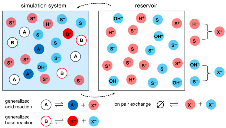
Figure 1: Schematic of an acid–base reaction system in equilibrium with a reservoir at a fixed pH and salinity. The acid (A) and base (B) groups can undergo ionization reactions, becoming charged (A^-, B⁺) via the release of ions ($\textnormal{H}^{+}$, $\textnormal{OH}^{-}$). Salt cations ($\textnormal{S}^{+}$) and anions ($\textnormal{S}^{-}$), as well as released ions, are exchanged between the system and the reservoir. In principle, all possible reactions that preserve the charge neutrality of the system must be considered. Grouping all free monovalent ions into a single particle type (X) markedly reduces the number of required reactions and increases MC sampling performance.

We consider charged particles immersed in an implicit solvent at constant temperature $T$. The particles can represent acidic groups (A), basic groups (B), dissociated ions ($\textnormal{H}^{+}$, $\textnormal{OH}^{-}$), free cations ($\textnormal{S}^{+}$), and free anions ($\textnormal{S}^{-}$) (Fig. 1). The following reactions may occur,

A $$\rightleftharpoons \textnormal{A}^{-}+\textnormal{H}^{+}\;,$$ (1)

B $$\rightleftharpoons \textnormal{B}^{+}+\textnormal{OH}^{-}\;,$$ (2)

where $\textnormal{A}^{-}$ and $\textnormal{B}^{+}$ denote the ionized states of the respective groups. We also take into account the self-dissociation of water,

$$\varnothing\rightleftharpoons\textnormal{H}^{+}+\textnormal{OH}^{-}\;,$$ (3)

where $\varnothing$ denotes an empty set since the solvent ($\textnormal{H}_{2}\textnormal{O}$) is not explicitly considered. The system is in equilibrium with a reservoir at a given salinity, which can be formally expressed as

$$\varnothing\rightleftharpoons\textnormal{S}^{+}+\textnormal{S}^{-}\;.$$ (4)

A natural choice to simulate the reactions Eqs. (1)–(4) is to employ the RxMC method [31, 32], which provides a framework for modeling arbitrary chemical reactions. However, this method is limited to physical reactions and consequently, as noted in Sec. I, implementing Eqs. (1)–(4) alone does not generally lead to the correct grand-canonical distribution of charged states [47], with strong finite-size effects when the concentration of one or more reacting particles is low, e.g., at $\textnormal{pH}\approx 7$.

This limitation of the RxMC method has recently been addressed in the grand-reaction method [50]. By including additional charge-neutral reactions, such as $\varnothing\rightleftharpoons\textnormal{H}^{+}+\textnormal{S}^{-}$, $\textnormal{A}\rightleftharpoons\textnormal{A}^{-}+\textnormal{S}^{+}$, the system is able to reach the correct equilibrium charge distribution. However, these additional reactions increase the implementation complexity as well as the computational cost of the method. There are now eight possible reactions in total, but depending on the system conditions, only a fraction of these reactions effectively sample the ionization states of the system. For example, at $\textnormal{pH}\approx 7$ a representative simulation volume $V<10^{7}\,\textnormal{nm}^{3}$ on average contains less than one $\textnormal{H}^{+}$ and $\textnormal{OH}^{+}$. Thus, most MC moves involving $\textnormal{H}^{+}$ and $\textnormal{OH}^{-}$ are rejected and only three out of the eight possible reactions are effective.

II.2 CR-MC method

The premise of our new method is that it is more efficient to consider generalized reactions in which all like-charged monovalent ions in solution are grouped into a single particle type. These groupings keep the number of required reactions low and thereby improve the MC sampling efficiency of CR. Thus, we implement CR with three general reactions,

A $$\rightleftharpoons \textnormal{A}^{-}+\textnormal{X}^{+}\;,$$ (5)

B $$\rightleftharpoons \textnormal{B}^{+}+\textnormal{X}^{-}\;,$$ (6)

$$\varnothing \rightleftharpoons \textnormal{X}^{+}+\textnormal{X}^{-}\;,$$ (7)

where the $\textnormal{X}^{\pm}$ denote monovalent free ions. In the acid dissociation reaction, Eq. (5), an acid group (A) is ionized by transferring a proton from the system to the reservoir, while simultaneously transferring an ion X⁺ from the reservoir to the system. If we choose X⁺ as the dissociated cation ($\textnormal{X}^{+}={\textnormal{H}^{+}}$) and X^- as the dissociated anion ($\textnormal{X}^{-}={\textnormal{OH}^{-}}$) this scheme exactly reduces to the RxMC method [31, 32], Eqs. (1)–(3). The scheme can be applied multiple times, separately to dissociated and salt ions within the same simulation, in which case it becomes equivalent to the recent grand-reaction ensemble method [50] discussed above.

Most coarse-grained electrolyte models, such as the restricted primitive model [51, 52], already routinely use the same interaction potentials for all monovalent ions, so that the grouping of all monovalent cations and protons into a single ion type, i.e., $\textnormal{X}^{+}=\{{\textnormal{H}^{+}},\,{\textnormal{S}^{+}}\}$, and likewise for all monovalent anions and hydroxyl groups, $\textnormal{X}^{-}=\{{\textnormal{OH}^{-}},\,{\textnormal{S}^{-}}\}$, is natural (Fig. 1). The grouping operation strictly preserves the correct grand-canonical distribution of charged states and does not affect any equilibrium properties of the system (Appendix A), but reduces the number of necessary reactions. For example, Eqs. (3) and (4), along with the “mixed” reactions $\varnothing\rightleftharpoons\textnormal{H}^{+}+\textnormal{S}^{-}$ and $\varnothing\rightleftharpoons\textnormal{OH}^{-}+\textnormal{S}^{+}$, are combined into a single MC step, Eq. (7). This grouping requires the interaction potential of all ions in the group to be the same. Thus, the grouping operation is not applicable in systems where differences in the short-range interaction of different ion types, such as Hofmeister-series effects, are important. The grouping also cannot be performed between ions of different valencies, but multivalent ions of a given valency can be grouped straightforwardly.

The chemical potentials $\mu_{\textnormal{X}^{+}}$ and $\mu_{\textnormal{X}^{-}}$ of the combined cation and the combined anion species, respectively, are determined through a transformation of the grand partition function (Appendix A),

$$e^{\beta\mu_{\textnormal{X}^{+}}} = e^{\beta\mu_{\textnormal{H}}}+e^{\beta\mu_{\textnormal{S}^{+}}}\;,$$ (8)

$$e^{\beta\mu_{\textnormal{X}^{-}}} = e^{\beta\mu_{\textnormal{OH}}}+e^{\beta\mu_{\textnormal{S}^{-}}}\;,$$ (9)

with $\beta=1/(k_{\textnormal{B}}T)$, $k_{\textnormal{B}}$ the Boltzmann constant, and $\mu_{\textnormal{H}}$, $\mu_{\textnormal{S}^{+}}$, $\mu_{\textnormal{OH}}$, and $\mu_{\textnormal{S}^{-}}$ the chemical potentials of the respective ionic species in the reservoir. Moreover, even if the (short-range) interaction potentials of $\textnormal{H}^{+}$ and $\textnormal{S}^{+}$ (or $\textnormal{OH}^{-}$ and $\textnormal{S}^{-}$) differ, Eqs. (8) and (9) are obtained in the dilute electrolyte limit where the details of the short-range ion–ion interaction are immaterial.

The CR-MC method, Eqs. (5)–(7), can also be applied simultaneously to association or adsorption of other ions, such as $\textnormal{Na}^{+}$, in which case B would refer to an empty surface site and $\textnormal{B}^{+}$ would be a site occupied by $\textnormal{Na}^{+}$.

II.3 Monte Carlo algorithm

To implement the scheme described, we derive the MC acceptance rate for the general CR reactions, Eqs. (5)–(7), within the framework of a grand-canonical ensemble. There are six possible MC moves, namely the forward and reverse move for each of the three CR reactions. Forward and reverse moves are proposed with equal probability, leading to the detailed balance condition

$$p_{\textnormal{o}}p^{\textnormal{acc}}_{\textnormal{o}\to\textnormal{n}}=p_{\textnormal{n}}p^{\textnormal{acc}}_{\textnormal{n}\to\textnormal{o}}\;,$$ (10)

where $p_{\textnormal{o}}$ ($p_{\textnormal{n}}$) is the equilibrium probability of the old (new) state and $p^{\textnormal{acc}}_{\textnormal{o}\to\textnormal{n}}$ ($p^{\textnormal{acc}}_{\textnormal{n}\to\textnormal{o}}$) the corresponding acceptance rate. Particles that participate in the reaction are chosen uniformly at random from all eligible particles in the system. If no suitable particles are available, a move is rejected automatically. For clarity, in the following we use the language of acid–base ionization equilibria, but the algorithm is general to any ionization process.

We assume that the simulated system contains a fixed number of $n_{\textnormal{A}}$ acidic groups and $n_{\textnormal{B}}$ basic groups with corresponding dissociation free energies $\Delta G_{\textnormal{a}}$ and $\Delta G_{\textnormal{b}}$, respectively. The number of free cations $n_{\textnormal{X}^{+}}$ and free anions $n_{\textnormal{X}^{-}}$ is allowed to fluctuate via the exchange of ions with the reservoir, which sets the temperature, the pH, and the chemical potentials of combined ions, $\mu_{\textnormal{X}^{+}}$ and $\mu_{\textnormal{X}^{-}}$. The equilibrium probability of the system being in a state with potential energy $E$, $n_{\textnormal{A}}^{-}$ (negatively charged) dissociated acid groups, and $n_{\textnormal{B}}^{+}$ (positively charged) base groups, along with $n_{\textnormal{X}^{-}}$ free anions and $n_{\textnormal{X}^{+}}$ cations, is

$$p(n_{\textnormal{A}^{-}},n_{\textnormal{B}^{+}},n_{\textnormal{X}^{+}},n_{\textnormal{X}^{-}},E) = \frac{n_{\textnormal{A}}!}{n_{\textnormal{A}^{-}}!(n_{\textnormal{A}}-n_{\textnormal{A}^{-}})!}e^{-\beta(\Delta G_{\textnormal{a}}+\mu_{\textnormal{H}})n_{\textnormal{A}^{-}}}\frac{n_{\textnormal{B}}!}{n_{\textnormal{B}^{+}}!(n_{\textnormal{B}}-n_{\textnormal{B}^{+}})!}e^{-\beta({\Delta G_{\textnormal{b}}+\mu_{\textnormal{OH}}})n_{\textnormal{B}^{+}}}$$ (11)

$$\times \frac{\left[\rho_{0}N_{\textnormal{A}}Ve^{\beta\mu_{\textnormal{X}^{+}}}\right]^{n_{\textnormal{X}^{+}}}}{n_{\textnormal{X}^{+}}!}\ \frac{\left[\rho_{0}N_{\textnormal{A}}V\,e^{\beta\mu_{\textnormal{X}^{-}}}\right]^{n_{\textnormal{X}^{-}}}}{n_{\textnormal{X}^{-}}!}\,\frac{e^{-\beta E}}{\Xi}\;.$$

The first four factors on the right-hand side capture the ionization and combinatorial entropy of acid and base groups, where $\mu_{\textnormal{H}}$ and $\mu_{\textnormal{OH}}$ determine the chemical potentials of dissociated cations ($\textnormal{H}^{+}$) and anions ($\textnormal{OH}^{-}$). The fifth and sixth factors represent the ideal partition functions of the free ions, where $\rho_{0}$ is the reference concentration, usually set to $\rho_{0}=1\,$M, $N_{\textnormal{A}}$ Avogadro’s number, and $V$ the system volume. $\Xi$ is the normalizing factor, i.e., the grand partition function of the system (see Appendix A).

The MC acceptance rates are obtained by inserting Eq. (11) into Eq. (10) where the “old” and “new” states correspond to the chosen reactions, Eqs. (5)–(7). To simplify the resulting expressions, we use a base-10 logarithmic representation for all chemical potentials and dissociation constants, $\textnormal{pI}_{\textnormal{X}^{\pm}}=-\beta\mu_{\textnormal{X}^{\pm}}\log_{10}e$, $\textnormal{pI}_{\textnormal{S}^{\pm}}=-\beta\mu_{\textnormal{S}^{\pm}}\log_{10}e$, $\textnormal{pH}=-\beta\mu_{\textnormal{H}}\log_{10}e$, and $\textnormal{pOH}=-\beta\mu_{\textnormal{OH}}\log_{10}e$, with $e$ Euler’s number. The chemical potential of the combined type in the reservoir is determined by the pH of the reservoir and $\textnormal{pI}_{\textnormal{S}^{\pm}}$ via $10^{-\textnormal{pI}_{\textnormal{X}^{+}}}=10^{-\textnormal{pH}}+10^{-\textnormal{pI}_{\textnormal{S}^{+}}}$ [see Appendix A and Eq. (31)]. Likewise, the dissociation constants are $\textnormal{p}K_{\textnormal{a}}=\beta\Delta G_{\textnormal{a}}\log_{10}e$ and $\textnormal{p}K_{\textnormal{b}}=\beta\Delta G_{\textnormal{b}}\log_{10}e$.

The forward acid reaction consists of three steps. An acid group becomes negatively charged, a dissociated ion ($\textnormal{H}^{+}$) is placed into the reservoir, and an ion $\textnormal{X}^{+}$ is taken from the reservoir and placed into the system. The corresponding acceptance ratio is

$$\frac{p^{\textnormal{acc}}_{(n_{\textnormal{A}^{-}})\to(n_{\textnormal{A}^{-}}+1)}}{p^{\textnormal{acc}}_{(n_{\textnormal{A}^{-}}+1)\to(n_{\textnormal{A}^{-}})}}=\frac{(n_{\textnormal{A}}-n_{\textnormal{A}^{-}})\rho_{0}N_{\textnormal{A}}V}{(n_{\textnormal{A}^{-}}+1)(n_{\textnormal{X}^{+}}+1)}10^{\textnormal{pH}-\textnormal{p}K_{\textnormal{a}}-\textnormal{pI}_{\textnormal{X}^{+}}}e^{-\beta\Delta E}\;,$$ (12)

with $\Delta E=E_{\textnormal{n}}-E_{\textnormal{o}}$ the difference in the potential energy of the new and the old state of the system. Thus, applying the Metropolis scheme, we obtain the acceptance probability for the forward acid reaction,

$$p^{\textnormal{acc}}_{(n_{\textnormal{A}^{-}})\to(n_{\textnormal{A}^{-}}+1)}=\min\left[1,\frac{(n_{\textnormal{A}}-n_{\textnormal{A}^{-}})\rho_{0}N_{\textnormal{A}}V}{(n_{\textnormal{A}^{-}}+1)(n_{\textnormal{X}^{+}}+1)}10^{\textnormal{pH}-\textnormal{p}K_{\textnormal{a}}-\textnormal{pI}_{\textnormal{X}^{+}}}e^{-\beta\Delta E}\right]\;.$$ (13)

Similarly, in the backward acid reaction an ion $\textnormal{X}^{+}$ is placed into the reservoir, an ion $\textnormal{H}^{+}$ is taken from the reservoir and placed into the system, and finally an acid group is neutralized. The corresponding acceptance probability is

$$p^{\textnormal{acc}}_{(n_{\textnormal{A}^{-}})\rightarrow(n_{\textnormal{A}^{-}}-1)}=\min\left[1,\frac{n_{\textnormal{A}^{-}}n_{\textnormal{X}^{+}}}{(n_{\textnormal{A}}-n_{\textnormal{A}^{-}}+1)\rho_{0}N_{\textnormal{A}}V}10^{-\textnormal{pH}+\textnormal{p}K_{\textnormal{a}}+\textnormal{pI}_{\textnormal{X}^{+}}}e^{-\beta\Delta E}\right]\;.$$ (14)

The forward/backward base reaction acceptance probabilities are

$$p^{\textnormal{acc}}_{(n_{\textnormal{B}^{+}})\rightarrow(n_{\textnormal{B}^{+}}+1)}=\min\left[1,\frac{\left(n_{\textnormal{B}}-n_{\textnormal{B}^{+}}\right)\rho_{0}N_{\textnormal{A}}V}{\left(n_{\textnormal{B}^{+}}+1\right)\left(n_{\textnormal{X}^{-}}+1\right)}10^{\textnormal{pOH}-\textnormal{p}K_{\textnormal{b}}-\textnormal{pI}_{\textnormal{X}^{-}}}e^{-\beta\Delta E}\right]\;$$ (15)

and

$$p^{\textnormal{acc}}_{(n_{\textnormal{B}^{+}})\rightarrow(n_{\textnormal{B}^{+}}-1)}=\min\left[1,\frac{n_{\textnormal{B}^{+}}n_{\textnormal{X}^{-}}}{\left(n_{\textnormal{B}}-n_{\textnormal{B}^{+}}+1\right)\rho_{0}N_{\textnormal{A}}V}10^{-\textnormal{pOH}+\textnormal{p}K_{\textnormal{b}}+\textnormal{pI}_{\textnormal{X}^{-}}}e^{-\beta\Delta E}\right]\;,$$ (16)

whereas the ion pair insertion/deletion probabilities are given by

$$p^{\textnormal{acc}}_{(n_{\textnormal{X}^{\pm}})\rightarrow(n_{\textnormal{X}^{\pm}}+1)}=\min\left[1,\frac{\left(\rho_{0}N_{\textnormal{A}}V\right)^{2}}{\left(n_{\textnormal{X}^{+}}+1\right)\left(n_{\textnormal{X}^{-}}+1\right)}10^{-\textnormal{pI}_{\textnormal{X}^{+}}-\textnormal{pI}_{\textnormal{X}^{-}}}e^{-\beta\Delta E}\right]\;$$ (17)

and

$$p^{\textnormal{acc}}_{(n_{\textnormal{X}^{\pm}})\rightarrow(n_{\textnormal{X}^{\pm}}-1)}=\min\left[1,\frac{n_{\textnormal{X}^{+}}n_{\textnormal{X}^{-}}}{\left(\rho_{0}N_{\textnormal{A}}V\right)^{2}}10^{\textnormal{pI}_{\textnormal{X}^{+}}+\textnormal{pI}_{\textnormal{X}^{-}}}e^{-\beta\Delta E}\right]\;.$$ (18)

II.4 Performance analysis

The computational cost of the CR-MC method is dominated by the evaluation of the energy $E$. When used with a long-range electrostatic solver, such as the particle–particle particle–mesh (PPPM) algorithm [53], each attempted MC moves requires one evaluation of the full system energy, provided that the energy of the original configuration was retained after a prior MC move or MD step. Likewise, each MD time step also requires a full calculation of long-range electrostatics, so that the computational cost of an MC move is comparable to that of a single MD step. The number of MC moves $n_{\textnormal{MC}}$ to be performed for every $n_{\textnormal{MD}}$ MD time steps depends on the simulation setup. If the objective is to sample equilibrium properties the main consideration is convergence to equilibrium and rapid decorrelation of configurations. The optimal ratio is determined by the decorrelation time scale of the system, which can be limited by either the MD or the MC aspect of the simulation, depending on the model parameters. However, a reasonable rule of thumb is to use $n_{\textnormal{MC}}\sim n_{\textnormal{MD}}$, thus ensuring comparable computational cost of the MC and MD components of the simulation. This choice guarantees that in all situations the number of evaluations of the long-range electrostatic energy is at most twice the optimal number and thereby yields an overall performance that is always a large fraction of the optimal performance. On the other hand, if the goal is to sample the correct dynamics of the dissociation/association process with specific dissociation rates, $n_{\textnormal{MC}}$ is set by these rates. For example, to model an acid with a given dissociation rate $r_{\textnormal{d}}$, the ratio of acid dissociation attempts $n^{\textnormal{A}}_{\textnormal{MC}}$ to MD steps should be on average $n^{\textnormal{A}}_{\textnormal{MC}}/n_{\textnormal{MD}}\approx n_{\textnormal{A}}r_{\textnormal{d}}\delta t$, with $\delta t$ the MD time step.

The evaluation of the system energy is dominated by the evaluation of the electrostatic energy. With a fast PPPM solver the computational complexity of each MD time step and each MC move scales as $\mathcal{O}(N\log N)$, with $N$ the number of charges in the system. Moreover, the total number of MC steps required to relax the charge distribution in the system scales approximately linearly with the number of ionizable sites $M$ in the system. The total computational complexity of MC sampling is thus $\mathcal{O}(MN\log N)$, which dominates over MD for large $M$. Therefore, an efficient MC algorithm is crucial to achieve an acceptable performance when simulating large systems. Our algorithm and implementation (Appendix B) make it possible to simulate CR phenomena in large systems containing tens of thousands of weak acid sites [12].

To obtain a representative performance comparison between different methods, we simulate a simple weak electrolyte consisting of $n_{\textnormal{A}}=500$ individual acidic groups ($\textnormal{p}K_{\textnormal{a}}=6.5$) immersed in an implicit solvent with a dielectric constant $\varepsilon$ within a periodic cubic box of size $L=50l_{\textnormal{B}}$ with $l_{\textnormal{B}}=q_{0}^{2}/(4\pi\varepsilon\varepsilon_{0}k_{\textnormal{B}}T)$ the Bjerrum length, $q_{0}$ the elementary charge, and $\varepsilon_{0}$ the vacuum permittivity. We consider an aqueous solution ($l_{\textnormal{B}}=0.72\,\textnormal{nm}$) with typical pH and salinity values, $\textnormal{pH}=7$ and $\textnormal{pI}_{\textnormal{S}^{\pm}}=2$, corresponding to a symmetric ($\textnormal{pI}_{\textnormal{S}^{\pm}}=\textnormal{pI}_{\textnormal{S}^{+}}=\textnormal{pI}_{\textnormal{S}^{-}}$) monovalent salt concentration $c\approx 0.01$ M. Since we aim to evaluate the performance of the CR algorithm, MD integration is not performed. Electrostatic interactions are taken into account via the PPPM algorithm with a relative force accuracy of $10^{-5}$ and real-space cutoff $r_{\text{cut}}=10l_{\textnormal{B}}$.

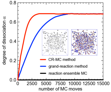
Figure 2: Convergence of the average degree of dissociation $\alpha$ obtained using three methods. The CR-MC method with ion grouping (red curve), the grand-reaction ensemble method (blue curve), and the conventional reaction-ensemble method (black curve), all of which can be realized using our LAMMPS implementation. The inset snapshot shows the simulated system of a simple weak acid electrolyte (see text for details). The CR-MC method results in the same thermodynamic equilibrium as the grand-reaction method, but significantly accelerates the convergence, whereas the reaction-ensemble method suffers from prohibitively strong finite-size effects and is unable to reach thermodynamic equilibrium. The data is averaged over 1000 independent runs. Parameters: $\textnormal{pH}=7$, $\textnormal{pI}_{\textnormal{S}^{\pm}}=2$, $\textnormal{p}K_{\textnormal{a}}=6.5$, $L=50l_{\textnormal{B}}$.

We compare the efficiency of our CR-MC method with the conventional RxMC [31, 32, 33] and the grand-reaction ensemble method [50] (Fig. 2). All three methods differ only in the types of MC moves that are used and are simulated with our LAMMPS implementation (see Appendix B). The three methods could also be simulated using the ESPResSo package which implements the RxMC and grand-reaction ensemble methods. The CR-MC method can be simulated in this package by defining rescaled chemical potentials [Eqs. (8) and (9)] and equilibrium constants that implement the generalized reactions [Eqs. (5)–(7)], i.e., the acid equilibrium constant $K_{\textnormal{A}}=10^{\textnormal{pH}-\textnormal{p}K_{\textnormal{a}}-\textnormal{pI}_{\textnormal{X}^{+}}}$, the base equilibrium constant $K_{\textnormal{B}}=10^{\textnormal{pOH}-\textnormal{p}K_{\textnormal{b}}-\textnormal{pI}_{\textnormal{X}^{-}}}$, and the electrolyte dissociation constant $K_{\textnormal{ion}}=10^{-\textnormal{pI}_{\textnormal{X}^{-}}-\textnormal{pI}_{\textnormal{X}^{+}}}$.

We examine the convergence of the degree of dissociation $\alpha=\langle n_{\textnormal{A}^{-}}\rangle/n_{\textnormal{A}}$ averaged over 1000 independent initial configurations that are generated by randomly placing individual neutral acid groups in the system while not allowing any overlaps, i.e., ensuring an inter-group distance $r_{ij}>\sigma 2^{1/6}$, for all particles in the system (Fig. 2 inset). The same random configurations are used with all three methods and initially no salt ions are present. The conventional RxMC does not result in the correct charge distribution due to severe finite-size effects [47] (Fig. 2, black curve). This issue is corrected by completing the set of possible MC moves, i.e., by employing the grand-reaction ensemble method [50] (Fig. 2, blue curve). Lastly, the CR-MC method (Fig. 2, red curve) converges to the same degree of dissociation, but approximately three times faster. In this comparison, all possible MC moves are attempted with the same probability. Since each MC step requires the evaluation of the total electrostatic energy—unless one or more reacting particles do not exist and the move is immediately rejected—the computational cost of a single MC step is expected to be very similar for all three methods. Indeed, we find that the average CPU time per MC step is the same for the CR-MC method and the grand-reaction ensemble method. Instead, the origin of the slower performance of the grand-reaction ensemble lies in the low concentration of H⁺, on average less than one H⁺ ion in the simulation box, causing most MC moves involving H⁺ to be rejected. Whereas this could be partially compensated by tuning the relative frequency of the different MC moves, we note that the grouping of all free monovalent ions of the same sign, as employed in CR-MC, is natural in coarse-grained electrolyte models, where these ions already routinely use the same interaction potentials.

The combined ions can at any time be ungrouped into their constituent subspecies. The probability $p_{i}$ that any ion belongs to a a given subspecies $i$ is $p_{i}=\exp(\beta\mu_{i})/\exp(\beta\mu_{\textnormal{X}})$. For example, for the combined cation $\textnormal{X}^{+}=\{\textnormal{H}^{+},\textnormal{S}^{+}\}$ a fraction $p_{\textnormal{S}^{+}}=10^{-\textnormal{pI}_{\textnormal{S}^{+}}+\textnormal{pI}_{\textnormal{X}^{+}}}$ of the $\textnormal{X}^{+}$ ions present in the simulation will represent salt cations $\textnormal{S}^{+}$ and a fraction $p_{\textnormal{H}^{+}}=10^{-\textnormal{pH}+\textnormal{pI}_{\textnormal{X}^{+}}}$ will represent $\textnormal{H}^{+}$ ions. The grouping of anions follows an equivalent approach. The grouping and ungrouping operation are exact in thermodynamic equilibrium. When simulating dynamics of non-equilibrium processes, the evolution of the system depends on the transport properties of individual ions and thus the grouping operation can no longer be applied indiscriminately. The grouping can still be applied in non-equilibrium situations if the configurational changes of simulated entities, e.g., polymers or nanoparticle aggregates, are slow compared to the relaxation of the ion density distribution, such that the ion distribution can be considered to be in quasi-equilibrium.

III Applications and discussion

III.1 Configurations of a hydrophobic weak polyelectrolyte

To demonstrate a practical application of the CR-MC method, we investigate the equilibrium configurations of a single hydrophobic polyelectrolyte (PE) chain consisting of $N_{\textnormal{m}}=80$ weak acid groups. All particles are modeled as spheres of diameter $\sigma=l_{\textnormal{B}}=0.72\,\textnormal{nm}$ that interact via a shifted-truncated Lennard-Jones (LJ) potential

$$U_{\textnormal{LJ}}(r_{ij})=\begin{cases}4\varepsilon_{\mathrm{LJ}}\left[\left(\frac{\sigma}{r_{ij}}\right)^{12}-\left(\frac{\sigma}{r_{ij}}\right)^{6}+C\right]&\;r_{ij}\leq r_{\textnormal{cut}}\\ 0&\;r_{ij}>r_{\textnormal{cut}}\;.\end{cases}$$ (19)

We use the standard cutoff $r_{\textnormal{cut}}=2.5\sigma$ and shift $C=2.5^{-6}-2.5^{-12}$ for intra-PE interactions to simulate hydrophobic effects, while all other short-range interactions are purely repulsive, namely $r_{\textnormal{cut}}=2^{1/6}\sigma$ and $C=1/4$. Table 1 summarizes the LJ interaction parameters, where the Lorentz–Berthelot mixing rule is used.

Table 1: Lennard-Jones parameters $\varepsilon_{\mathrm{LJ}}$, $r_{\textnormal{cut}}$ [Eq. (19)] for the hydrophobic PE system. We set $\sigma=l_{\textnormal{B}}$ and $\varepsilon_{\textnormal{ii}}=k_{\textnormal{B}}T$. The subscripts “i” and “m” refer to ions and monomers, respectively.

type	acid monomer	free ion
acid monomer	$\varepsilon_{\textnormal{mm}}$, $2.5\sigma$	$\sqrt{\varepsilon_{\textnormal{mm}}\varepsilon_{\textnormal{ii}}}$, $2^{1/6}\sigma$
free ion	$\sqrt{\varepsilon_{\textnormal{mm}}\varepsilon_{\textnormal{ii}}}$, $2^{1/6}\sigma$	$\varepsilon_{\textnormal{ii}}$, $2^{1/6}\sigma$

Neighboring monomers along the chain are bonded through a harmonic potential,

$$U_{\textnormal{bond}}(r_{ij})=K({r_{ij}}-R_{0})^{2}\;,$$ (20)

with spring constant $K=400k_{\textnormal{B}}T/{\sigma}^{2}$ and bond length $R_{0}=2^{1/6}\sigma$. The relatively large spring constant ensures that the intra-chain electrostatic repulsion cannot noticeably affect the contour length of the chain. The PE is simulated in a periodic cubic box with dimensions $L=100l_{\textnormal{B}}$. Electrostatic interactions are treated in the same manner as in Sec. II.4. The temperature is controlled by a Langevin thermostat with damping time $\tau=[m\sigma^{2}/(k_{\textnormal{B}}T)]^{1/2}$, where $m$ is the ion mass. The positions and velocities are updated using the velocity-Verlet algorithm with a time step of $\delta t=0.005\tau$. After every $n_{\textnormal{MD}}=400$ MD steps, we perform $n_{\textnormal{MC}}=200$ MC steps. We start from a random configuration and equilibrate the system for $10^{3}\tau$. The subsequent production runs last for $2\times 10^{5}\tau$, during which the configurations are sampled every $20\tau$.

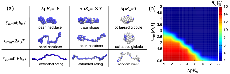
Figure 3: Equilibrium conformations of a hydrophobic weak polyelectrolyte. (a) Representative configurations at different dissociation strength $\Delta\textnormal{p}K_{\textnormal{a}}=\textnormal{p}K_{\textnormal{a}}-\textnormal{pH}$ and short-range (hydrophobic) attraction $\varepsilon_{\textnormal{mm}}$. Charged bead are shown in blue and neutral beads in white. Free ions are not shown for better visualization of the PE conformations. (b) The corresponding radius of gyration $R_{\text{g}}$ shows an abrupt transition between extended (large $R_{\textnormal{g}}$, red shading) and collapsed (low $R_{\textnormal{g}}$, blue shading) structures. In all cases we used $\textnormal{pH}=7$ and $\textnormal{pI}_{\textnormal{S}^{\pm}}=3$.

The competition between the electrostatic monomer repulsion, which promotes polymer expansion, and the short-range monomer attraction representing hydrophobicity, which promotes collapse, leads to a rich conformational behavior of a hydrophobic PE chain. Indeed, by tuning the values of $\Delta\textnormal{p}K_{\textnormal{a}}=\textnormal{p}K_{\textnormal{a}}-\text{pH}$ and the monomer attraction $\varepsilon_{\textnormal{mm}}$ we reproduce the five types of structures reported in earlier simulation work [35], namely the random walk, extended string, collapsed globule, “cigar shape,” and pearl-necklace conformations (Fig. 3a).

In the case of strong dissociation, $\Delta\textnormal{p}K_{\textnormal{a}}=-6$, the PE chain is nearly fully charged and exhibits the well-known conformations of strong PEs, from a pearl-necklace structure at strong attraction (large $\varepsilon_{\textnormal{mm}}$) to an extended string-like structure at weaker attraction (Fig. 3a, left column). At intermediate degrees of dissociation, $\Delta\textnormal{p}K_{\textnormal{a}}=-3.7$, the polyelectrolyte is only partially charged, leading to weaker electrostatic repulsion and consequently more compact structures, such as a “cigar”-shaped structure (Fig. 3a, middle column). Furthermore, weak dissociation, $\Delta\textnormal{p}K_{\textnormal{a}}=0$, leads to a largely uncharged PE. Under these conditions, the chain collapses into a globule at strong monomer attraction, but behaves as a neutral, random coil at weak attraction (Fig. 3a, right column).

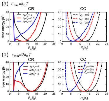
Figure 4: Free-energy profiles as a function of $R_{\textnormal{g}}$ for a hydrophobic weak polyelectrolyte exhibit two stable minima, which indicates the coil–globule transition detected in Fig. 3(b) is discontinuous (solid lines), while the corresponding constant-charge (CC) approximation (dashed lines) results in a single minimum. In (a) and (b), we set $\varepsilon_{\textnormal{mm}}=1.0k_{\textnormal{B}}T$ and $\varepsilon_{\textnormal{mm}}=2.0k_{\textnormal{B}}T$, respectively.

We note that the average radius of gyration $R_{\text{g}}$ characterizing these conformations displays an abrupt change in the parameter space span by $\varepsilon_{\textnormal{mm}}$ and $\Delta\textnormal{p}K_{\textnormal{a}}$ (Fig. 3b). As our CR-MC method is implemented in LAMMPS, it can be directly combined with standard free-energy methods. Thus, we examine the nature of the variation in shape by calculating the free-energy profiles as a function of $R_{\textnormal{g}}$. We apply the metadynamics method [54] implemented in the COLVARS library [55] of LAMMPS, using a bin size $0.05\sigma$ and a “Gaussian-hill” weight $0.005k_{\textnormal{B}}T$, with hills deposited every $10$ MD time steps. We find that under CR conditions the free-energy profile exhibits two minima at the transition point (Fig. 4), indicating a coil–globule transition that is first order (with the caveat that a true thermodynamic transition would require the limit of infinite chain length). Prior theoretical [56] and simulation [57] investigations indeed suggested that CR effects could lead to a first-order coil–globule transition of weak PEs, but to our knowledge this is the first time that this has been confirmed by a free-energy calculation. Repeating the simulations in the corresponding CC approximation, where each chain bead has a fixed charge $Q_{\textnormal{a}}/N_{\textnormal{m}}$ ($Q_{\textnormal{a}}$ the average charge of the weak PE obtained from an equilibrium CR simulation), we always find a single free-energy minimum. Thus, while the observed structures are not new, CR leads to transitions between these structures that are qualitatively different from those observed in the conventional CC approximation.

III.2 Potential of mean force between charged nanoparticles

Charge regulation effects have been shown to reduce the electrostatic repulsion between like-charged particles [7, 8] and increase the attraction between a large particle coated with dissociable sites and a small ion [12]. However, the interaction between two oppositely charged particles has not been explored in detail, even though this arrangement provides a prototypical model for investigating CR effects on electrostatic protein–protein interactions [3, 4, 5].

As an illustration, we calculate the potential of mean force (PMF) between two oppositely charged nanoparticles of radius $R=3.5l_{\textnormal{B}}$ immersed in an implicit aqueous solvent characterized by $l_{\textnormal{B}}=0.72$ nm and $\textnormal{pH}=7$. The solution also contains free ions (salt, protons, and hydroxyl ions) of diameter $\sigma=l_{\textnormal{B}}$. The weak acid and weak base groups on the surface of the nanoparticles have dissociation constants $\textnormal{p}K_{\textnormal{a}}=\textnormal{p}K_{\textnormal{b}}=6.5$. A set of 256 acid/base groups is uniformly distributed on, and rigidly attached to, the shell (radius $3l_{\textnormal{B}}$) of each sphere [12]. We examine two salt concentrations, namely $\textnormal{pI}_{\textnormal{S}^{\pm}}=6$, $c\approx 10^{-6}$ M, representing deionized water, and $\textnormal{pI}_{\textnormal{S}^{\pm}}=1$, $c\approx 0.1$ M, representing a physiological saline solution. In the former case, we utilize a system size $L=1000l_{\textnormal{B}}$ and in the latter $L=40l_{\textnormal{B}}$. This ensures that the number of free ions in the solution greatly exceeds the charge on the individual nanoparticles, thus avoiding spurious long-range electrostatic interactions between periodic images. The excluded-volume interactions are modeled through the expanded LJ potential,

$$U_{\textnormal{LJ}}(r_{ij})=\begin{cases}4\varepsilon_{\mathrm{LJ}}\left[\left(\frac{\sigma}{{r_{ij}}-\Delta}\right)^{12}-\left(\frac{\sigma}{{r_{ij}}-\Delta}\right)^{6}+\frac{1}{4}\right]&\;r_{ij}\leq r_{\textnormal{c}}^{*}\\ 0&\;r_{ij}>r_{\textnormal{c}}^{*}\,,\end{cases}$$ (21)

with $\Delta$ the expanded distance and $r_{\textnormal{c}}^{*}=\Delta+2^{1/6}\sigma$ the cutoff. The interaction parameters for the different combinations of particle types are listed in Table 2.

Table 2: Lennard-Jones interaction parameters in the system of colloidal nanoparticles (radius $R$) and free ions (radius $r$). We always use $\varepsilon_{\mathrm{LJ}}=k_{\textnormal{B}}T$, $\sigma=2r$, and cutoff $r_{\text{c}}^{*}=\Delta+2^{1/6}\sigma$.

type	particle $(R)$	free ions $(r)$
particle $(R)$	$\Delta=2R-2r$	$\Delta=R-r$
free ions $(r)$	$\Delta=R-r$	$\Delta=0$

The temperature $T$ is controlled by a Langevin thermostat with damping time $20\tau$, where the unit time $\tau$ (Sec. III.1) is based upon the mass $m$ of the ions and dissociable groups. The total nanoparticle mass is $257m$. After equilibrating the system for $5\times 10^{3}\tau$, the production runs last for $5\times 10^{5}\tau$ with MD time step $\delta t=0.005\tau$. After every $400$ MD steps, we perform $200$ MC steps.

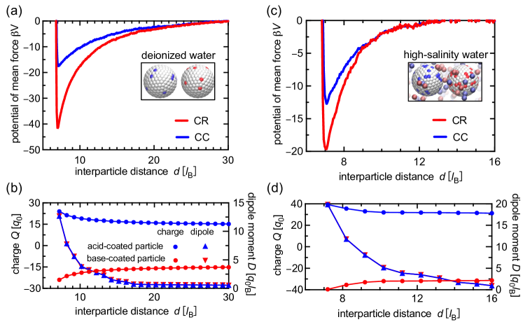
Figure 5: Effect of charge regulation on the interactions between two oppositely charged nanoparticles, modeled as an acid-coated and a base-coated particle. The respective dissociation constants are $\textnormal{p}K_{\textnormal{a}}=6.5$ and $\textnormal{p}K_{\textnormal{b}}=6.5$, while the pH is fixed at $7$. (a) Potential of mean force (PMF) between the charge regulating (CR) particles (red curve) and comparison to the constant charge (CC) approximation (blue curve), when the particles are immersed in deionized water ($\textnormal{pI}_{\textnormal{S}^{\pm}}=6$). Inset shows a typical configuration of an acid-coated particle displaying dissociated (blue) and neutral (white) acid groups, accompanied by a base-coated particle with positively charged (red) and neutral (white) base groups. In the CC simulation, the particle charges are $Q_{\textnormal{acid}}=-Q_{\textnormal{base}}=-14q_{0}$ , obtained from the equilibrium surface charge of isolated particles ($d\to\infty$). (b) Variation of the total charge on the acid-coated (blue circles) and the base-coated (red circles) CR nanoparticle with varying separation $d$. The total dipole moment of both particles is shown as well (blue and red triangles, respectively). (c) Counterpart of panel (a), showing the PMF of the nanoparticle pair immersed in physiological saline solution ($\textnormal{pI}_{\textnormal{S}^{\pm}}=1$). In this case, the particle charge in the CC case is $Q_{\textnormal{acid}}=-Q_{\textnormal{base}}=-29q_{0}$. Inset shows a typical configuration, now also featuring free cations (light red) and anions (light blue). (d) Counterpart of panel (b), illustrating the variation of nanoparticle charge with separation at $\textnormal{pI}_{\textnormal{S}^{\pm}}=1$. Panels (b) and (d) demonstrate that the enhanced attraction of nanoparticles under CR conditions originates from the increased net charge at short separations as well as the nonuniform distribution of the ionized surface groups. Further computational details are provided in the main text.

To investigate the role of CR effects, we calculate the PMF of two colloidal nanoparticles using the metadynamics technique described in Sec. III.1 and compare it to the PMF in the CC approximation. The latter is realized by placing single charges $Q_{\textnormal{acid}}$ and $Q_{\textnormal{base}}$, obtained from independent simulations of isolated acid-coated and base-coated nanoparticles at the above-mentioned conditions, at their respective centers of mass. The PMF profiles (Fig. 5a,c) show that CR can enhance pairwise interactions about twofold compared to the CC situation. This enhancement is a result of both the change in the average charge per particle and the nonuniform surface-charge distribution characterized by the induced dipole moment (Fig. 5b,d). Notably, the enhancement of pairwise interactions by CR not only occurs in deionized water (Fig. 5a,b), but persists at physiological salt concentration ((Fig. 5c,d). This is markedly different from dielectric effects, which are effectively screened under such conditions [58, 59]. This example illustrates that CR effects must be generally taken into account when modeling bio-macromolecular interactions that typically occur at physiological salt conditions.

IV Summary

We have introduced the CR-MC method, a MC scheme that makes possible the efficient and accurate calculation of charge regulation in solvated systems. The method is most suitable for coarse-grained models with implicit solvent, where the details of the short-range ion–ion interaction, such as Hofmeister-series effects, can be neglected. By grouping all like-charged free monovalent ions into a single particle type and allowing monovalent salt to participate in acid–base reactions, our CR-MC method outperforms previous approaches (constant-pH method [29, 30], RxMC [31, 32, 33], and grand-RxMC method [50]) in applicable parameter range or efficiency.

We have implemented the CR-MC method within the LAMMPS [49] MD package. The implementation is parallelized and compatible with existing LAMMPS functionalities, such as rigid-body dynamics and free-energy calculations, and thus markedly lowers the entry barrier to incorporating charge regulation effects into MD simulations. We emphasize that this enables self-consistent calculations in which the instantaneous distribution of particles and charges determines the electrostatic forces that drive the time evolution of the system, and conversely the resulting distributions affect the charge states of the particles. The LAMMPS implementation also supports RxMC [31, 32, 33] and grand-RxMC [50] methods.

We have demonstrated the capabilities of our approach by determining the conformations of a hydrophobic weak polyelectrolyte for different dissociation conditions as well as the corresponding free-energy profiles as a function of its radius of gyration. We found that CR effects lead to the coexistence of two stable states at the coil–globule transition, implying a discontinuous coil–globule transition, thus corroborating previous predictions [57]. Interestingly, this discontinuous transition vanishes in the usual CC approximation that ignores the fluctuations of individual charges on the polyelectrolyte. As a second example, we calculated the PMF between an acid-coated and a base-coated colloidal nanoparticle, demonstrating that CR effects give rise to an approximately twofold increase in the attractive interaction at both low and high salinity. These examples show that CR effects can markedly alter the behavior of charged systems and demonstrate the importance of an accurate CR solver.

The CR-MC method allows the modeling of simple reactions and charge redistribution in a broad range of coarse-grained, solvated systems, such as polyelectrolytes, proteins, membranes, and nanoparticles. Although we have focused on simulating acid–base ionization equilibria, the method is general and can be used to model any two-state association/dissociation process.

Data Availability

The data that support the findings of this study are available within the article. The source code of our CR-MC implementation is available via the standard LAMMPS repository, see Appendix B.

Appendix A Derivation of the grand-canonical ensemble with ion grouping

We show that the proposed grouping of different ions, which is at the core of the efficiency gain provided by the CR-MC method, within the primitive electrolyte model preserves the correct grand-canonical distribution of concentrations and leads to Eq. (11). The grand-canonical ensemble of states for a system with volume $V$ and temperature $T$ in contact with a reservoir containing $M$ different particle types is determined by $M$ chemical potentials $\mu_{i}$, denoted in vector notation as $\bm{\mu}=[\mu_{1},\cdots,\mu_{M}]$. The grand-canonical partition function describing this ensemble,

$$\Xi(\bm{\mu},V,T)=\sum_{\mathbf{N}=0}^{\infty}e^{\beta\bm{\mu}\cdot\mathbf{N}}Q(\mathbf{N},V,T)\;,$$ (22)

is obtained by summing over all $\mathbf{N}=[N_{1},\cdots,N_{M}]$ possible numbers of particles of each type in the system, where the summation denotes a nested sum, $\sum_{\mathbf{N}}[\cdot]=\sum_{N_{1}}\sum_{N_{2}}\cdots\sum_{N_{M}}[\cdot]$, and $\beta=1/(k_{\textnormal{B}}T)$ with $k_{\textnormal{B}}$ the Boltzmann constant. The canonical partition function,

$$Q(\mathbf{N},V,T)=\prod_{l=1}^{M}\frac{1}{N_{l}!}\left(\frac{V}{\Lambda^{3}}\right)^{N_{l}}\mathcal{I}(\mathbf{N},V,T)\;,$$ (23)

contains the product performed over the ideal-gas contributions of individual particle types, with the reference length scale $\Lambda=(\rho_{0}N_{\textnormal{A}})^{-1/3}$ set by the reference concentration $\rho_{0}=1\;\textnormal{M}$. The configurational contribution,

$$\mathcal{I}(\mathbf{N},V,T)=\int d\mathbf{r}^{N}e^{-\beta E(\mathbf{r}^{N})}\;,$$ (24)

is obtained by integrating over the positions of all $N=\sum_{l}N_{l}$ particles in the system, with $E(\mathbf{r}^{N})$ the potential energy of the system that depends on the positions $\mathbf{r}$ of all $N$ particles.

Within the primitive model electrolyte, all monovalent ions use the same short-range interaction potential. Therefore, exchanging one cation type for another cation type leaves the potential energy of the system unchanged. For example, if type $i$ represents $\textnormal{H}^{+}$, type $j$ represents salt cation $\textnormal{S}^{+}$, and $N_{i}>0$, the configuration integral is invariant under changing of ion types,

$$\mathcal{I}([\cdot,N_{i},N_{j},\cdot],V,T)=\mathcal{I}([\cdot,N_{i}-1,N_{j}+1,\cdot],V,T)\;.$$ (25)

Therefore, by induction, $\mathcal{I}$ is a function only of the sum $N_{i}+N_{j}$,

$$\mathcal{I}=\mathcal{I}([\cdot,N_{i}+N_{j},\cdot],V,T)\;.$$ (26)

Using this property and Eq. (23) we rewrite Eq. (22) as

$$\Xi(\bm{\mu},V,T)=\sum_{\mathbf{N^{\prime}}=0}^{\infty}e^{\beta\bm{\mu}^{\prime}\cdot\mathbf{N^{\prime}}}\prod_{l\neq i,j}^{M}\left[\frac{1}{N_{l}!}\left(\frac{V}{\Lambda^{3}}\right)^{N_{l}}\right]\mathcal{S}\;,$$ (27)

where $\bm{\mu}^{\prime}$ and $\mathbf{N}^{\prime}$ contain all particle types except for $i$ and $j$ and $\mathcal{S}$ denotes the sum over elements $i$ and $j$,

$$\mathcal{S}=\sum_{N_{i}=0}^{\infty}\sum_{N_{j}=0}^{\infty}\frac{e^{\beta\mu_{i}N_{i}+\beta\mu_{j}N_{j}}}{N_{i}!N_{j}!}\left(\frac{V}{\Lambda^{3}}\right)^{N_{i}+N_{j}}\mathcal{I}\;.$$ (28)

This sum can be rewritten as a sum over $N_{\textnormal{X}}=N_{i}+N_{j}$,

$$\mathcal{S}=\sum_{N_{\textnormal{X}}=0}^{\infty}\sum_{N_{i}=0}^{N_{\textnormal{X}}}\frac{e^{\beta\mu_{i}N_{i}+\beta\mu_{j}(N_{\textnormal{X}}-N_{i})}}{N_{i}!(N_{\textnormal{X}}-N_{i})!}\left(\frac{V}{\Lambda^{3}}\right)^{N_{\textnormal{X}}}\mathcal{I}\;.$$ (29)

Since $\mathcal{I}$ does not explicitly depend on $N_{i}$, the inner sum can be recognized as a binomial expansion and Eq. (29) can be written as

$$\mathcal{S}=\sum_{N_{\textnormal{X}}=0}^{\infty}\left(e^{\beta\mu_{i}}+e^{\beta\mu_{j}}\right)^{N_{\textnormal{X}}}\frac{1}{N_{\textnormal{X}}!}\left(\frac{V}{\Lambda^{3}}\right)^{N_{\textnormal{X}}}\mathcal{I}\;.$$ (30)

This represents the grand-canonical partition function of a combined type X with chemical potential

$$\mu_{\textnormal{X}}=k_{\textnormal{B}}T\ln\left[e^{\beta\mu_{i}}+e^{\beta\mu_{j}}\right]\;.$$ (31)

Insertion of Eq. (30) into Eq. (27) yields a reduced partition function in $M-1$ particle types that is identical to the original full partition function in $M$ particle types, Eq. (22). Thus, the CR-MC method, Eqs. (12)–(18), which samples the statistical ensemble with combined ion types, Eq. (11), leads to exactly the same equilibrium observables as a Monte Carlo scheme (e.g., the scheme of Ref. 50) in which all ions are treated separately.

Appendix B LAMMPS implementation and usage

We have implemented the CR-MC method described in Sec. II.2 within the LAMMPS MD package. Our implementation is open source and distributed under the GNU General Public License (GPL). It is available from the central LAMMPS repository (https://lammps.sandia.gov/), including documentation and examples.

This LAMMPS implementation performs MC sampling of ionization states [Eqs. (13)–(18)]. The only input parameters required are the equilibrium constants ($\textnormal{p}K$), chemical potentials (pH, pOH) of dissociated ions, and the chemical potential of inserted ions, $\textnormal{pI}_{\textnormal{X}^{+}}$ and $\textnormal{pI}_{\textnormal{X}^{-}}$. The implementation is general. For example, choosing $\textnormal{pI}_{\textnormal{X}^{+}}=\textnormal{pH}$ and $\textnormal{pI}_{\textnormal{X}^{-}}=\textnormal{pOH}$ would perform canonical sampling of standard reactions [Eqs. (1)–(3)] following the RxMC approach for a closed system. The method can be invoked repeatedly to perform reactions with different types of ions within a single simulation, thus enabling simulation in the grand-reaction ensemble. To set up the CR-MC method presented in this work in our LAMMPS implementation, the dissociated ions and salt ions are combined into a single types of cations $\textnormal{X}^{+}$ and anions $\textnormal{X}^{-}$, cf. Eq. (31). Moreover, the implementation supports setting a variable (i.e., time-dependent) pH of the reservoir and can thus, for example, be used to study the response of a system to an increase in pH.

Appendix C Numerical validation

To confirm the correct functioning of our CR-MC implementation, we simulate weak acid dissociation over a wide range of parameters and compare our results to the grand-reaction ensemble approach [50] implemented in the ESPResSo MD package [48] (version 4.0.2). We examine a test system containing $n_{\textnormal{A}}=100$ acid groups immersed in an aqueous solution at room temperature. We set $L=30l_{\textnormal{B}}$, resulting in a similar density of acid groups as in Sec. II.4. All other interaction and system parameters are also described in Sec. II.4.

We explore the behavior of the system at non-neutral pH values, $\textnormal{pH}\neq\textnormal{pOH}$. In this case, charge neutrality of the reservoir implies that the chemical potentials of cations and anions (other than $\textnormal{H}^{+}$ and $\textnormal{OH}^{-}$) in the reservoir are different and must be specified separately. We assume that a non-neutral pH is obtained using a small monovalent acid or base, e.g., HCl or NaOH, which allows us to group the free negatively charged acid with the other monovalent anions into a single particle type, and likewise to group the free positively charged base with free cations. The chemical potential (in the $\log_{10}$ representation) of these additional acid anions ($\textnormal{pI}_{\textnormal{A}^{-}}$) is related to the pH, $10^{-\textnormal{pI}_{\textnormal{A}^{-}}}=10^{-\textnormal{pI}_{\textnormal{S}^{\pm}}}+10^{-\textnormal{pH}}-10^{-\textnormal{pOH}}$. Likewise, for basic solutions the chemical potential of the additional base cations ($\textnormal{pI}_{\textnormal{B}+}$) is determined by $10^{-\textnormal{pI}_{\textnormal{B}^{+}}}=10^{-\textnormal{pI}_{\textnormal{S}^{\pm}}}+10^{-\textnormal{pOH}}-10^{-\textnormal{pH}}$. Using the grouping operation [Eq. (31)] the chemical potential of the combined ion type is thus determined by $\textnormal{pI}_{\textnormal{S}^{\pm}}$ and pH via

$$10^{-\textnormal{pI}_{\textnormal{X}^{\pm}}}=10^{-\textnormal{pI}_{\textnormal{S}^{\pm}}}+10^{-\min[\textnormal{pH},\,\textnormal{pOH}]}\;,$$ (32)

where the first term on the right-hand side takes into account the symmetric monovalent salt, while the second term captures the dissociated ions as well as any free acid/base groups or ions that must be present to maintain a charge-neutral solution at a non-neutral pH.

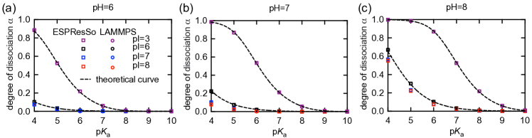
Figure 6: Average degree of dissociation $\alpha$ of monomeric acid groups as a function of $\textnormal{p}K_{\textnormal{a}}$. Data are shown for different values of $\textnormal{pI}=\textnormal{pI}_{\textnormal{S}^{\pm}}$, which determines the chemical potential of monovalent salt, and at three different pH (panels a–c). Square symbols are obtained by the grand-reaction method [50], which simulates the full set of six reactions in the ESPResSo MD package. Circles represent data obtained by the CR-MC method described in this work and implemented in LAMMPS. For all parameters considered, the two data sets show perfect agreement. The simulation data are further validated by a numerical approach that assumes ideal solution conditions and couples the Gibbs–Donnan equilibrium to the Henderson–Hasselbalch ionization equilibrium (dashed lines at $\textnormal{pI}=3$ and $\textnormal{pI}=6$).

In the numerical comparison, the temperature is controlled by a Langevin thermostat with damping time $\tau$. The positions and velocities are updated using the velocity-Verlet algorithm with time step $\delta t=0.01\tau$. After every $n_{\textnormal{MD}}=400$ MD steps we perform $n_{\textnormal{MC}}=200$ MC steps. We start from a random configuration and equilibrate the system for $10^{3}\tau$. The subsequent production runs last for $2\times 10^{5}\tau$, during which the configuration averages are sampled every $20\tau$, yielding the average degree of dissociation $\alpha$ (Fig. 6). As expected, increasing $\Delta\textnormal{p}K_{\textnormal{a}}=\textnormal{p}K_{\textnormal{a}}-\textnormal{pH}$ results in a lower $\alpha$, whereas adding more salt (decreasing $\textnormal{pI}_{\textnormal{S}^{\pm}}$) promotes acid dissociation as the additional salt screens the electrostatic repulsion between charged acid groups. In all cases, our implementation produces results that are statistically identical to those obtained using the ESPResSo package. We find our LAMMPS implementation to be about three times faster per MC step, which we attribute primarily to the CR-MC implementation requiring a single electrostatic energy evaluation per MC move, whereas the current reaction ensemble implementation in ESPResSo (version 4.0.2) calls the full energy evaluation twice per MC move. We emphasize that this difference in execution time per MC step is in addition to the more rapid decorrelation of the configurations resulting from the improved sampling of the CR-MC method (Fig. 2). The combined effect of these two enhancements results in an approximately 9-fold acceleration.

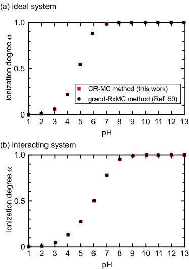
Figure 7: Comparison with previously published results. Average degree of dissociation $\alpha$ obtained using the CR-MC method with the LAMMPS implementation (squares) and previously published results that use the grand-reaction ensemble method with the ESPResSo package (circles) [Fig. 3 in Ref. 50]. (a) Ideal system without particle–particle interactions. (b) Interacting system of polyelectrolyte chains.

Lastly, we test the CR-MC method and LAMMPS implementation by reproducing previously published results on acid dissociation (Fig. 7). For this comparison we use dissociation constant $\textnormal{p}K_{\textnormal{a}}=4$, salt chemical potential $\textnormal{pI}_{\textnormal{S}^{\pm}}=2$, ion diameter $\sigma=0.355\,\textnormal{nm}$, Bjerrum length $l_{\textnormal{B}}=2\sigma$, box size $L=29.14l_{\textnormal{B}}$, and a total simulation time of $5\times 10^{5}\tau$ with time step $\delta t=0.005\tau$. We consider an ideal system of 800 monomers (Fig. 7a) as well as a polyelectrolyte solution containing 16 polyelectrolyte chains where each chain contains $N=50$ acid monomers bonded with a FENE potential (Fig. 7b) (see Supporting Information of Ref. 50, Section S3 for more details). In both cases we find that our calculation of the average degree of dissociation $\alpha$ is statistically identical results to the previously published data.

References

- Atkins and de Paula [2006] P. Atkins and J. de Paula, Physical Chemistry, 7th ed. (Oxford University Press, Oxford, U.K., 2006).
- Ninham and Parsegian [1971] B. W. Ninham and V. A. Parsegian, “Electrostatic potential between surfaces bearing ionizable groups in ionic equilibrium with physiologic saline solution,” J. Theor. Biol. 31, 405–428 (1971).
- Lund and Jönsson [2005] M. Lund and B. Jönsson, “On the charge regulation of proteins,” Biochemistry 44, 5722–5727 (2005).
- Lund and Jönsson [2013] M. Lund and B. Jönsson, “Charge regulation in biomolecular solution,” Q. Rev. Biophys. 46, 265–281 (2013).
- Roosen-Runge et al. [2014] F. Roosen-Runge, F. Zhang, F. Schreiber, and R. Roth, “Ion-activated attractive patches as a mechanism for controlled protein interactions,” Sci. Rep. 4, 7016 (2014).
- Lund, Åkesson, and Jönsson [2005] M. Lund, T. Åkesson, and B. Jönsson, “Enhanced protein adsorption due to charge regulation,” Langmuir 21, 8385–8388 (2005).
- Takae and Tanaka [2018] K. Takae and H. Tanaka, “Hydrodynamic simulations of charge-regulation effects in colloidal suspensions,” Soft Matt. 14, 4711–4720 (2018).
- dos Santos and Levin [2019] A. P. dos Santos and Y. Levin, “Like-charge attraction between metal nanoparticles in a electrolyte solution,” Phys. Rev. Lett. 122, 248005 (2019).
- Tagliazucchi, Olvera de la Cruz, and Szleifer [2010] M. Tagliazucchi, M. Olvera de la Cruz, and I. Szleifer, “Self-organization of grafted polyelectrolyte layers via the coupling of chemical equilibrium and physical interactions,” Proc. Natl. Acad. Sci. U.S.A. 107, 5300–5305 (2010).
- Barr and Panagiotopoulos [2012] S. A. Barr and A. Z. Panagiotopoulos, “Conformational transitions of weak polyacids grafted to nanoparticles,” J. Chem. Phys. 137, 144704 (2012).
- Kirkwood and Shumaker [1952] J. G. Kirkwood and J. B. Shumaker, “The influence of dipole moment fluctuations on the dielectric increment of proteins in solution,” Proc. Natl. Acad. Sci. U.S.A. 38, 855–862 (1952).
- Curk and Luijten [2021] T. Curk and E. Luijten, “Charge regulation effects in nanoparticle self-assembly,” Phys. Rev. Lett. 126, 138003 (2021).
- Yameen et al. [2009] B. Yameen, M. Ali, R. Neumann, W. Ensinger, W. Knoll, and O. Azzaroni, “Synthetic proton-gated ion channels via single solid-state nanochannels modified with responsive polymer brushes,” Nano Letters 9, 2788–2793 (2009).
- Guo et al. [2010] W. Guo, H. Xia, F. Xia, X. Hou, L. Cao, L. Wang, J. Xue, G. Zhang, Y. Song, D. Zhu, Y. Wang, and L. Jiang, “Current rectification in temperature-responsive single nanopores,” Chem. Phys. Chem. 11, 859–864 (2010).
- Tagliazucchi, Rabin, and Szleifer [2013] M. Tagliazucchi, Y. Rabin, and I. Szleifer, “Transport rectification in nanopores with outer membranes modified with surface charges and polyelectrolytes,” ACS Nano 7, 9085–9097 (2013).
- Huang et al. [2019] L. Huang, H. Zhang, S. Wu, X. Xu, L. Zhang, H. Ji, L. He, Y. Qian, Z. Wang, Y. Chen, J. Shen, Z.-W. Mao, and Z. Huang, “Charge regulation of self-assembled tubules by protonation for efficiently selective and controlled drug delivery,” iScience 19, 224–231 (2019).
- Walker et al. [2011] D. A. Walker, B. Kowalczyk, M. Olvera de la Cruz, and B. A. Grzybowski, “Electrostatics at the nanoscale,” Nanoscale 3, 1316–1344 (2011).
- Boles, Engel, and Talapin [2016] M. A. Boles, M. Engel, and D. V. Talapin, “Self-assembly of colloidal nanocrystals: From intricate structures to functional materials,” Chem. Rev. 116, 11220–11289 (2016).
- Zhou and Pang [2018] H.-X. Zhou and X. Pang, “Electrostatic interactions in protein structure, folding, binding, and condensation,” Chem. Rev. 118, 1691–1741 (2018).
- Majee et al. [2019] A. Majee, M. Bier, R. Blossey, and R. Podgornik, “Charge regulation radically modifies electrostatics in membrane stacks,” Phys. Rev. E 100, 050601 (2019).
- Trefalt, Behrens, and Borkovec [2016] G. Trefalt, S. H. Behrens, and M. Borkovec, “Charge regulation in the electrical double layer: Ion adsorption and surface interactions,” Langmuir 32, 380–400 (2016).
- Markovich, Andelman, and Podgornik [2016] T. Markovich, D. Andelman, and R. Podgornik, “Charge regulation: A generalized boundary condition?” Europhys. Lett. 113, 26004 (2016).
- Bakhshandeh, Frydel, and Levin [2020] A. Bakhshandeh, D. Frydel, and Y. Levin, “Charge regulation of colloidal particles in aqueous solutions,” Phys. Chem. Chem. Phys. 22, 24712–24728 (2020).
- Netz [2002] R. R. Netz, “Charge regulation of weak polyelectrolytes at low- and high-dielectric-constant substrates,” J. Phys.: Condens. Matter 15, S239–S244 (2002).
- Prusty et al. [2020] D. Prusty, R. J. Nap, I. Szleifer, and M. Olvera de la Cruz, “Charge regulation mechanism in end-tethered weak polyampholytes,” Soft Matt. 16, 8832–8847 (2020).
- Podgornik [2018] R. Podgornik, “General theory of charge regulation and surface differential capacitance,” J. Chem. Phys. 149, 104701 (2018).
- Lu and Zhang [2008] Z. Lu and Y. Zhang, “Interfacing ab initio quantum mechanical method with classical Drude osillator polarizable model for molecular dynamics simulation of chemical reactions,” J. Chem. Theory Comput. 4, 1237–1248 (2008).
- Maurer and Iftimie [2010] P. Maurer and R. Iftimie, “Combining ab initio quantum mechanics with a dipole-field model to describe acid dissociation reactions in water: First-principles free energy and entropy calculations,” J. Chem. Phys. 132, 074112 (2010).
- Reed and Reed [1992] C. E. Reed and W. F. Reed, “Monte Carlo study of titration of linear polyelectrolytes,” J. Chem. Phys. 96, 1609–1620 (1992).
- Radak et al. [2017] B. K. Radak, C. Chipot, D. Suh, S. Jo, W. Jiang, J. C. Phillips, K. Schulten, and B. Roux, “Constant-pH molecular dynamics simulations for large biomolecular systems,” J. Chem. Theory Comput. 13, 5933–5944 (2017).
- Smith and Triska [1994] W. R. Smith and B. Triska, “The reaction ensemble method for the computer simulation of chemical and phase equilibria. I. Theory and basic examples,” J. Chem. Phys. 100, 3019–3027 (1994).
- Johnson, Panagiotopoulos, and Gubbins [1994] J. K. Johnson, A. Z. Panagiotopoulos, and K. E. Gubbins, “Reactive canonical Monte Carlo,” Mol. Phys. 81, 717–733 (1994).
- Turner et al. [2008] C. H. Turner, J. K. Brennan, M. Lísal, W. R. Smith, J. K. Johnson, and K. E. Gubbins, “Simulation of chemical reaction equilibria by the reaction ensemble Monte Carlo method: A review,” Mol. Simul. 34, 119–146 (2008).
- Barr and Panagiotopoulos [2011] S. A. Barr and A. Z. Panagiotopoulos, “Interactions between charged surfaces with ionizable sites,” Langmuir 27, 8761–8766 (2011).
- Ulrich, Laguecir, and Stoll [2005a] S. Ulrich, A. Laguecir, and S. Stoll, “Titration of hydrophobic polyelectrolytes using Monte Carlo simulations,” J. Chem. Phys. 122, 094911 (2005a).
- Carnal, Ulrich, and Stoll [2010] F. Carnal, S. Ulrich, and S. Stoll, “Influence of explicit ions on titration curves and conformations of flexible polyelectrolytes: A Monte Carlo study,” Macromolecules 43, 2544–2553 (2010).
- Narayanan Nair, Uyaver, and Sun [2014] A. K. Narayanan Nair, S. Uyaver, and S. Sun, “Conformational transitions of a weak polyampholyte,” J. Chem. Phys. 141, 134905 (2014).
- Landsgesell, Holm, and Smiatek [2017] J. Landsgesell, C. Holm, and J. Smiatek, “Simulation of weak polyelectrolytes: A comparison between the constant pH and the reaction ensemble method,” Eur. Phys. J. Special Topics 226, 725–736 (2017).
- Murmiliuk et al. [2018] A. Murmiliuk, P. Košovan, M. Janata, K. Procházka, F. Uhlík, and M. Štěpánek, “Local pH and effective pK of a polyelectrolyte chain: Two names for one quantity?” ACS Macro Lett. 7, 1243–1247 (2018).
- Rathee et al. [2019] V. S. Rathee, H. Sidky, B. J. Sikora, and J. K. Whitmer, “Explicit ion effects on the charge and conformation of weak polyelectrolytes,” Polymers 11, 183 (2019).
- Ulrich, Laguecir, and Stoll [2005b] S. Ulrich, A. Laguecir, and S. Stoll, “Complexation of a weak polyelectrolyte with a charged nanoparticle. Solution properties and polyelectrolyte stiffness influences,” Macromolecules 38, 8939–8949 (2005b).
- Ulrich et al. [2006] S. Ulrich, M. Seijo, A. Laguecir, and S. Stoll, “Nanoparticle adsorption on a weak polyelectrolyte. Stiffness, pH, charge mobility, and ionic concentration effects investigated by Monte Carlo simulations,” J. Phys. Chem. B 110, 20954–20964 (2006).
- Carnal and Stoll [2011] F. Carnal and S. Stoll, “Adsorption of weak polyelectrolytes on charged nanoparticles. Impact of salt valency, pH, and nanoparticle charge density. Monte Carlo simulations,” J. Phys. Chem. B 115, 12007–12018 (2011).
- Stornes, Linse, and Dias [2017] M. Stornes, P. Linse, and R. S. Dias, “Monte Carlo simulations of complexation between weak polyelectrolytes and a charged nanoparticle. Influence of polyelectrolyte chain length and concentration,” Macromolecules 50, 5978–5988 (2017).
- Stornes, Shrestha, and Dias [2018] M. Stornes, B. Shrestha, and R. S. Dias, “pH-dependent polyelectrolyte bridging of charged nanoparticles,” J. Phys. Chem. B 122, 10237–10246 (2018).
- Hofzumahaus, Hebbeker, and Schneider [2018] C. Hofzumahaus, P. Hebbeker, and S. Schneider, “Monte Carlo simulations of weak polyelectrolyte microgels: pH-dependence of conformation and ionization,” Soft Matt. 14, 4087–4100 (2018).
- Landsgesell et al. [2019] J. Landsgesell, L. Nová, O. Rud, F. Uhlík, D. Sean, P. Hebbeker, C. Holm, and P. Košovan, “Simulations of ionization equilibria in weak polyelectrolyte solutions and gels,” Soft Matt. 15, 1155–1185 (2019).
- Limbach et al. [2006] H. J. Limbach, A. Arnold, B. A. Mann, and C. Holm, “ESPResSo—an extensible simulation package for research on soft matter systems,” Comput. Phys. Commun. 174, 704–727 (2006).
- Plimpton [1995] S. Plimpton, “Fast parallel algorithms for short-range molecular dynamics,” J. Comp. Phys. 117, 1–19 (1995).
- Landsgesell et al. [2020] J. Landsgesell, P. Hebbeker, O. Rud, R. Lunkad, P. Košovan, and C. Holm, “Grand-reaction method for simulations of ionization equilibria coupled to ion partitioning,” Macromolecules 53, 3007–3020 (2020).
- Valleau and Cohen [1980] J. P. Valleau and L. K. Cohen, “Primitive model electrolytes. I. Grand canonical Monte Carlo computations,” J. Chem. Phys. 72, 5935–5941 (1980).
- Luijten, Fisher, and Panagiotopoulos [2002] E. Luijten, M. E. Fisher, and A. Z. Panagiotopoulos, “Universality class of criticality in the restricted primitive model electrolyte,” Phys. Rev. Lett. 88, 185701 (2002).
- Hockney and Eastwood [1988] R. W. Hockney and J. W. Eastwood, Computer Simulation Using Particles (IOP Publishing, Bristol, 1988).
- Laio and Parrinello [2002] A. Laio and M. Parrinello, “Escaping free-energy minima,” Proc. Natl. Acad. Sci. U.S.A. 99, 12562–12566 (2002).
- Fiorin, Klein, and Hénin [2013] G. Fiorin, M. L. Klein, and J. Hénin, “Using collective variables to drive molecular dynamics simulations,” Mol. Phys. 111, 3345–3362 (2013).
- Raphael and Joanny [1990] E. Raphael and J.-F. Joanny, “Annealed and quenched polyelectrolytes,” Europhys. Lett. 13, 623–628 (1990).
- Uyaver and Seidel [2003] S. Uyaver and C. Seidel, “First-order conformational transition of annealed polyelectrolytes in a poor solvent,” Europhys. Lett. 64, 536–542 (2003).
- Antila and Luijten [2018] H. S. Antila and E. Luijten, “Dielectric modulation of ion transport near interfaces,” Phys. Rev. Lett. 120, 135501 (2018).
- Yuan, Antila, and Luijten [2020] J. Yuan, H. S. Antila, and E. Luijten, “Structure of polyelectrolyte brushes on polarizable substrates,” Macromolecules 53, 2983–2990 (2020).