A Statistical Detection of Wide Binary Systems in the Ultra-Faint Dwarf Galaxy Reticulum II

Abstract

Binary stars can inflate the observed velocity dispersion of stars in dark matter dominated systems such as ultra-faint dwarf galaxies (UFDs). However, the population of binaries in UFDs is poorly constrained by observations, with preferred binary fractions for individual galaxies ranging from a few percent to nearly unity. Searching for wide binaries through nearest neighbor (NN) statistics (or the two-point correlation function) has been suggested in the literature, and we apply this method for the first time to detect wide binaries in a UFD. By analyzing the positions of stars in Reticulum II (Ret II) from Hubble Space Telescope images, we search for angularly resolved wide binaries in Ret II. We find that the distribution of their NN distances shows an enhancement at projected separations of $\lesssim 1\arcsec$ relative to a model containing no binaries. We show that such an enhancement can be explained by a wide binary fraction of $f_{b}\approx 0.007^{+0.008}_{-0.003}$ at separations of more than 3000 AU. Under the assumption that the binary separation distribution is similar to that in the Milky Way, the total binary fraction in Ret II may be on the order of 50%. We also use the observed magnitude distribution of stars in Ret II to constrain the initial mass function over the mass range $0.34-0.78~{}{\rm\,M_{\odot}}$, finding that a shallow power-law slope of $1.01\leq\alpha\leq 1.15$ matches the data.

1. Introduction

Ultra-faint dwarf galaxies (UFDs) are the lowest luminosity galaxies known, with $L<10^{5}L_{\odot}$. UFDs are dark matter-dominated systems with ancient stellar populations (e.g., Simon & Geha, 2007; Geha et al., 2009; Brown et al., 2014; Li et al., 2018; Simon, 2019; Sacchi et al., 2021), which have been discovered at a rapid rate over the past 15 years by the Dark Energy Survey and other wide-field imaging surveys (e.g., Willman et al., 2005; Zucker et al., 2006; Belokurov et al., 2006; Bechtol et al., 2015; Koposov et al., 2015). Being relics of the early universe, UFDs have challenged various theories of dark matter, from the standard collisionless dark matter picture (Nadler et al., 2021), to ultra-light (fuzzy) dark matter (Calabrese & Spergel, 2016; Safarzadeh & Spergel, 2020; Burkert, 2020; Hayashi et al., 2021) and MOND (McGaugh & Wolf, 2010; Safarzadeh & Loeb, 2021).

The inferred dark matter masses and densities of dwarf galaxies are obtained through measurements of the line of sight velocity dispersion (e.g., Aaronson, 1983; Kleyna et al., 2005; Simon & Geha, 2007; Wolf et al., 2010). However, these measurements are in principle susceptible to the presence of binary stars. For binary stellar systems in UFDs, the primary mass has an upper limit of $0.8~{}M_{\odot}$ (because more massive stars have evolved into compact objects), while a typical companion mass is $\approx 0.3-0.5~{}M_{\odot}$ for an M dwarf and $\approx 0.6~{}M_{\odot}$ for a white dwarf. A binary system of $0.8$ and $0.5~{}M_{\odot}~{}$ stars with a period of 100 years will have a circular velocity on the order of a few $\,{\rm km\,s}^{-1}$.

Such binaries can inflate the inferred velocity dispersion of the galaxy (McConnachie & Côté, 2010; Simon et al., 2011; Kirby et al., 2013a, 2017; Ji et al., 2016; Spencer et al., 2018; Simon, 2019, although see Minor et al. 2010). The recent determination that the close binary fraction (at separations less than 10 AU) in the Milky Way varies inversely with metallicity, reaching 50% at $\textrm{[Fe/H]}=-3$ (Badenes et al., 2018; Moe et al., 2019), increases the importance of this issue for very metal-poor systems such as UFDs. On the other hand, the wide binary fraction (separation $>1000$ AU) may decrease toward lower metallicity (Hwang et al., 2021, although see El-Badry & Rix 2019), but no measurements are available for stars as metal-poor as those in UFDs.

Many recent studies attempt to minimize the effect of close binaries by identifying and removing them from kinematic samples using velocity measurements with a time baseline of $\sim 1$ yr (e.g., Fu et al., 2019; Jenkins et al., 2020; Buttry et al., 2021). However, somewhat wider binaries may evade detection if their velocity changes by less than $2-3~{}\,{\rm km\,s}^{-1}$ in this time interval. An alternative approach is to trace the population of binary stars through the distribution of the projected separations between the stars (Peñarrubia et al., 2016; Kervick et al., 2021). This idea has been explored conceptually, but not examined with real data as it requires high quality imaging with spatial resolution comparable to the expected separations of wide binaries. The angular separations, in turn, depend on the distance to the UFD and the intrinsic distribution of projected binary separations. Moreover, in order to obtain a reliable statistical inference of the binary fraction, the imaging must be deep enough or the galaxy must be luminous enough to make a large sample of member stars available. Given the combined considerations of distance, luminosity, and imaging coverage, we identify Reticulum II (Ret II) as an intriguing target for detecting wide binaries. Ret II is located at a distance of $31.4\pm 1.4$ kpc (Mutlu-Pakdil et al., 2018), and recent Hubble Space Telescope (HST) imaging of the galaxy provides a sample of $\sim 2600$ member stars. At the distance of Ret II, a binary system with a projected separation of 1 pc will have an angular separation of 6$\farcs$7. The HST diffraction limit at optical wavelengths of $\sim 0.1\arcsec$ corresponds to a physical scale of 0.015 pc (3000 AU). With the observed separation distribution of wide binaries (spanning from $\sim 10-10^{5}$ AU) in the solar neighborhood (El-Badry et al., 2021), $\sim 3\%$ of binary pairs should be resolvable at the distance of Ret II. For the first time, we analyze the statistics of nearest neighbors in Ret II in search of enhancements at close separations that could be explained by the presence of the binaries. The structure of this paper is as follows: in §2, we discuss Ret II and the data used for our analysis. In §3, we explain how we model the distribution of the stars as an ellipsoid and how magnitudes are assigned to the stars. In §4, we discuss our result and constraints on the derived binary fraction of Ret II based on fitting the NN distribution, and we investigate the initial mass function in Ret II using the observed magnitude distribution.

2. TARGET AND OBSERVATIONS

2.1. Properties of Reticulum II

Ret II is a typical UFD, with an absolute magnitude of $M_{V}=-3.1$ ($L=1500~{}L_{\odot}$) and a half-light radius of 58 pc (Mutlu-Pakdil et al., 2018). The important physical parameters for our analysis are its angular size and ellipticity, both of which affect the projected separations between random (physically unassociated) pairs of member stars. Published values for these properties are: $R_{h}=6\farcm 0\pm 0\farcm 6$, $\epsilon=0.6^{+0.1}_{-0.2}$ (Bechtol et al., 2015), $R_{h}=3\farcm 6^{+0\farcm 2}_{-0\farcm 1}$, $\epsilon=0.59^{+0.02}_{-0.03}$ (Koposov et al., 2015), $R_{h}=5\farcm 4\pm 0\farcm 2$, $\epsilon=0.56\pm 0.03$ (Muñoz et al., 2018), $R_{h}=6\farcm 3\pm 0\farcm 4$, $\epsilon=0.6\pm 0.1$ (Mutlu-Pakdil et al., 2018), and $R_{h}=6\farcm 6\pm 0\farcm 2$, $\epsilon=0.60\pm 0.01$ (Moskowitz & Walker, 2020). The latter three studies use deeper and more uniform photometry than the discovery papers, but the results across all five structural analyses are in reasonable agreement apart from the small size determined by Koposov et al. (2015). To ensure consistency with our modeling procedures described in §3, we perform our own fits to both the DES DR1 (Abbott et al., 2018) data set employed by Muñoz et al. (2018) and Moskowitz & Walker (2020) and the Megacam photometry from Mutlu-Pakdil et al. (2018). Following the methodology described by Drlica-Wagner et al. (2020) and Simon et al. (2021) and fitting with an exponential profile, we find $R_{h}=5\farcm 9^{+0\farcm 4}_{-0\farcm 3}$, $\epsilon=0.61\pm 0.03$ with the DES data and $R_{h}=6\farcm 2\pm 0\farcm 3$, $\epsilon=0.60\pm 0.03$ with the Megacam data. As representative measurements from the deepest available data, we adopt the Mutlu-Pakdil et al. (2018) values of $R_{h}=6\farcm 3$ and (when needed) $\epsilon=0.6$ for the remainder of this paper.

2.2. HST Imaging

Reticulum II was observed with the Wide Field Channel of the Advanced Camera for Surveys (ACS; Ford et al.) on the Hubble Space Telescope (HST) for program GO-14766 (PI: Simon). The data consist of 12 image tiles, each of which was observed for one orbit that was split between the F606W and F814W filters. Data reduction and photometry followed the procedures described by Brown et al. (2014) and Simon et al. (2021), using DAOPHOT-II (Stetson, 1987) to carry out point-spread function fitting in the STMAG system. Further details about the data and processing will be provided in a forthcoming paper analyzing the star formation history of Ret II with the same data set (J. D. Simon et al., in prep.).

We select Ret II member stars in the ACS color-magnitude diagram (CMD) based on a PARSEC isochrone track (Bressan et al., 2012; Chen et al., 2014; Marigo et al., 2017) with an age of 13 Gyr (similar to previously studied UFDs; Brown et al. 2014) and a metallicity of $\textrm{[Fe/H]}=-2.65$ (Simon et al., 2015). We use a selection window in color space that extends 0.15 mag bluer than the isochrone, except for the magnitude range near the main sequence turnoff, where the window is expanded to 0.40 mag to include the blue stragglers. To the red side, the selection window is 0.15 mag for stars brighter than $m_{814}=22$, and gradually widens to 0.45 mag at $m_{814}=26.5$. We limit the member sample to magnitudes brighter than $m_{814}=26.5$ to avoid the much greater levels of contamination and incompleteness that set in at fainter magnitudes.

We remove sources with bad DAOPHOT photometry flags or spatial profiles that are not consistent with a point source. However, stars whose fluxes could be contaminated by neighboring objects are not removed from the sample, in order to avoid discarding true binaries. For the goals of this study, small photometric errors that may result from stars with close and/or bright neighbors are unimportant. In order to avoid artifacts from bright, saturated stars, we also eliminate detected objects that are within 5″ of $G<11$ stars in the Gaia eDR3 catalog (Gaia Collaboration et al., 2016, 2021a), within 3″ of $11\leq G<15$ stars, or within 1″ of $15\leq G<17$ stars. Finally, we check for and remove sources with multiple slightly offset detections (which result from astrometric distortions in ACS) in the small overlap regions between tiles. After this cleaning, the total number of presumed Ret II member stars is 2587. In Figure 1, we display the spatial distribution of this sample of stars with the ACS tiling pattern overlaid.

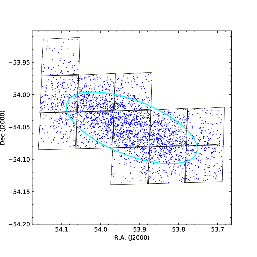
Figure 1.— Spatial distribution of Ret II stars in the ACS data set. The 12 ACS pointings are outlined in black, and an ellipse marking the half-light radius of Ret II is shown in cyan.

2.3. Distribution of Nearest Neighbor Distances

In the left panel of Figure 2, we compare the observed distribution of nearest neighbor (NN) distances for the stars in Ret II (black histogram) with a simulated population of stars with the same geometry as Ret II: an exponential profile with a half-light radius of 6$\farcm$3 and $\epsilon=0.6$ (red histogram). The construction of this model is described in more detail below (§ 3.1), and in the example shown here the model contains no binary stars. We notice that the NN distribution of the stars in Ret II exhibits a possible excess of pairs with small separations compared to what an ellipsoidal reconstruction of Ret II without binaries yields. Could this difference be due to the presence of wide binaries? In the right panel of Figure 2, we compare the Ret II NN distribution with models with a non-zero binary fraction to show that the data are sensitive to this quantity.

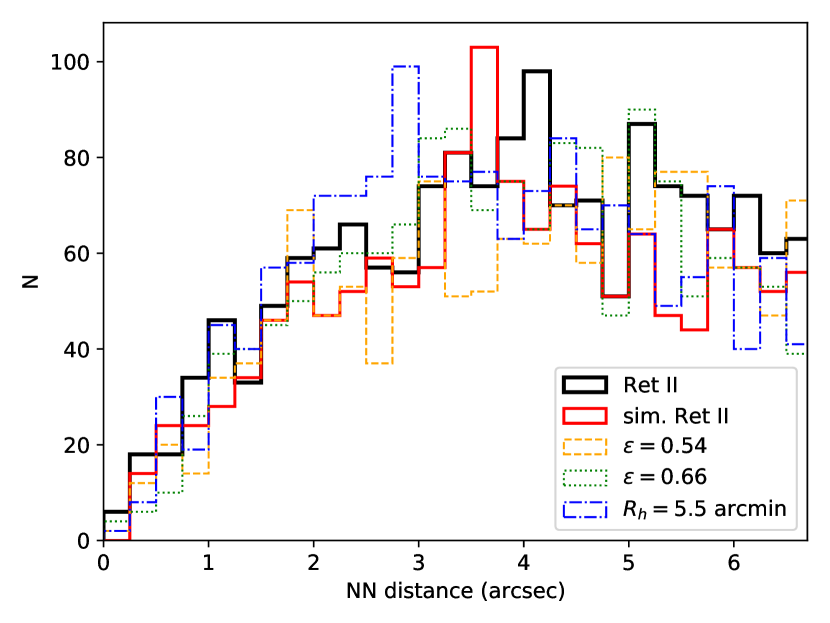
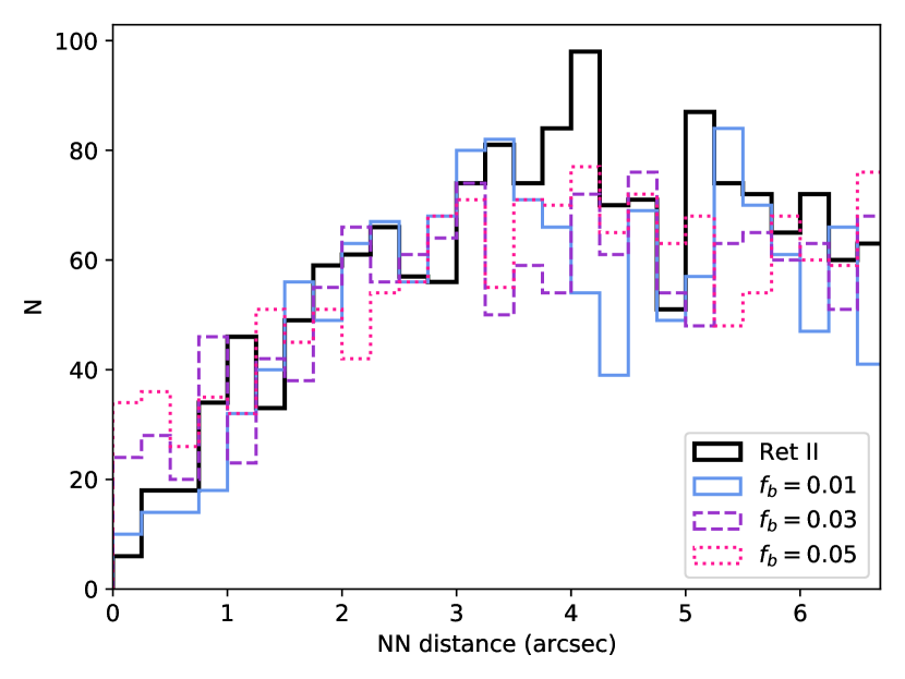
Figure 2.— (Left) Comparison of the nearest neighbor (NN) distance for Ret II stars (black histogram) with mock data sets created by varying the assumed geometry of the galaxy, with no binaries. The red histogram uses the adopted parameters for Ret II, and the orange, green, and blue histograms vary the assumed ellipticity or half-light radius. The mock data generally exhibit fewer pairs of stars at the smallest separations than Ret II does. (Right) Comparison of the nearest neighbor (NN) distance for Ret II stars (black histogram) with mock data sets created by varying the assumed wide binary fraction. Wide binary fractions of 3% and 5% are clearly inconsistent with the data at separations of less than 1″.

3. Methods

3.1. Constructing a Model Galaxy with Binary Stars

We construct a 3D ellipsoidal model of a Ret II-like system based on the assumed half-light radius of $R_{h}=6\farcm 3$ and ellipticity of $\epsilon=0.6$. Assuming an exponential profile for Ret II, we first project the surface density to a 3D radial profile through Abel’s integral:

$$j(r)=-\frac{1}{\pi}\int_{r}^{\infty}\frac{dR}{\sqrt{R^{2}-r^{2}}}\frac{dI}{dR},$$ (1)

where $I(R)$ is the surface density profile, modeled as $I(R)\propto e^{-R/R_{e}}$. Here, $R_{e}$ is the projected exponential scale radius, which is related to the projected half-light radius by $R_{e}=R_{h}/1.68$. The radial distances of the stars in the model galaxy are sampled from $r^{2}j(r)$, and the projected $x,y$ positions of the stars in an elliptical distribution are given by:

$$x=r\sin(\theta)\cos(\phi),~{}y=(1-e)~{}r\sin(\theta)\sin(\phi),$$ (2)

where $\phi$ is sampled uniformly between $(0,2\pi)$, and $\cos(\theta)$ is sampled uniformly between $(0,1)$.

When including a population of binary stars in the model (with binary fraction $f_{b}$), the positions of the primary stars are modeled as above, and the positions of the secondary stars are given by:

$$x_{s}=x_{p}+d\cos(\eta),~{}y_{s}=y_{p}+d\cos(\zeta)\sin(\eta),$$ (3)

where the “p” and “s” subscripts refer to the primary and secondary stars in a binary system, respectively, and $d$ is the projected separation sampled from a power-law distribution $p(d)\propto d^{\beta}$ The inclination angle $(\zeta)$ is sampled uniformly in $\cos(\zeta)$ between $(0,1)$, and the binary phase ($\eta$) is sampled uniformly between $(0,2\pi)$.

To match the geometry of the observational data set, we rotate the coordinate system to the position angle of Ret II and remove stars that fall outside the outline of the HST mosaic displayed in Fig. 1. Both the single stars and binaries that are removed through this step are replaced by an equal number of additional stars (drawn from the distributions described above) located within the HST footprint.

3.2. Assigning Magnitudes to Single and Binary Stars

We assign a mass to each simulated star assuming a Kroupa (2001) initial mass function (IMF). For the primary stars, we include stars between the mass limits of 0.2 and 0.8 ${\rm\,M_{\odot}}$ (lower-mass stars are not detectable in the HST data, while more massive stars are no longer present in Ret II because of its old age). For secondary stars, we define their masses to follow the derived mass ratio distribution from the analysis of binaries in the Milky Way (Kouwenhoven et al., 2009; Chulkov, 2021; El-Badry et al., 2019):

$$p(q)=\dfrac{dN}{dq}\sim\begin{cases}p_{\gamma}(q),~{}0\leq q<q_{\rm twin}\\ 1,~{}q_{\rm twin}\leq q\leq 1\\ \end{cases}$$ (4)

where

$$p_{\gamma}\left(q\right)\propto\left(\frac{q}{q_{\rm break}}\right)^{\gamma_{\rm smallq}}\left[1+\left(\frac{q}{q_{\rm break}}\right)^{1/\Delta}\right]^{\left(\gamma_{\rm largeq}-\gamma_{\rm smallq}\right)\Delta}.$$ (5)

We adopt $q_{\rm break}=0.5$, and $\Delta=0.3$. The other parameters, $\gamma_{\rm smallq}$, $\gamma_{\rm largeq}$, $q_{\rm twin}$, and $F_{\rm twin}$ depend on the primary mass of the star in the binary and the projected separation of the binaries. We adopt values for these parameters from Table G1 of El-Badry et al. (2019), where there is no evidence for changes as a function of projected separation ($d$) in the range $d>3000$ AU probed by our data, so we use a single average number for each parameter rather than allowing them to vary. $q_{\rm twin}$ determines the mass ratio above which there is an excess of twin binaries, and $F_{\rm twin}$ is a measure of the relative abundance of the twin binaries to all binaries in a given bin of primary star mass and binary separation. Most relevant for Ret II are the numbers associated with primary masses between $0.6\leq M_{p}\leq 0.8~{}{\rm\,M_{\odot}}$ and $0.4\leq M_{p}\leq 0.6~{}{\rm\,M_{\odot}}$ for separations between $50\leq d/{\rm AU}\leq 350$. Figure 3 shows random draws from the mass ratio distribution for the two mass bins we consider.

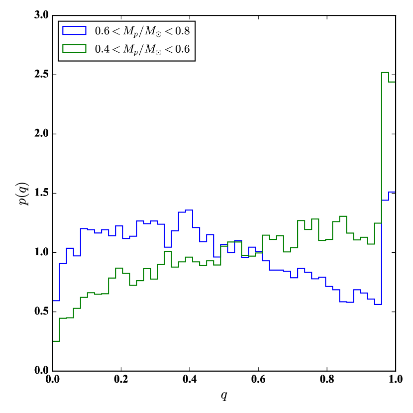
Figure 3.— Realizations of the distribution of binary mass ratios ($q$) for two separate mass bins of $0.4\leq M_{p}\leq 0.6~{}{\rm\,M_{\odot}}$, and $0.6\leq M_{p}\leq 0.8~{}{\rm\,M_{\odot}}$. The parameters describing the mass ratio distributions are adopted from El-Badry et al. (2019). The sharp peak at $q=1$ is due to the excess of twin binaries observed in the solar neighborhood.

We determine absolute magnitudes for the simulated stars based on their stellar masses by interpolating the same PARSEC isochrone employed in § 2 for member selection. We convert the absolute magnitudes into apparent magnitudes assuming a distance of 31.4 kpc (Mutlu-Pakdil et al., 2018) and extinction values of $A_{F606W}=0.045$ mag and $A_{F814W}=0.028$ mag (Schlafly & Finkbeiner, 2011). For binary systems that are unresolved by HST, we combine the magnitudes of the primary and secondary stars. For resolved binaries where the secondary star is fainter than our magnitude limit, we include only the primary magnitude.

3.3. Nearest Neighbor Distribution and MCMC Fits

We then determine the NN separation of each star in the simulated dwarf galaxy. At the wavelength of the F606W filter, the angular resolution of HST is $\sim 0\farcs 1$, so we treat binaries with projected NN separation less than $0\farcs 1$ as single stars. Doing so reduces the number of simulated stars, and to compensate for it we add new single stars to the galaxy so that the total number of simulated stars matches the total number of stars in the Ret II data, which is $n_{T}=2587$.

After computing the projected NN distances for the simulated dwarf galaxy stars, we bin the data into $0\farcs 5$-wide bins for separations up to 15″, with the observed data binned in the same way.

The model presented in §3.1 contains a total of four parameters: the half-light radius and ellipticity of the galaxy, the binary fraction ($f_{b}$), and the slope ($\beta$) of the power-law distribution of binary separations in AU. Because the half-light radius is well-determined from the photometric data, and because it would be computationally inefficient to evaluate the integral in Equation 1 in each Monte Carlo iteration, we adopt a fixed value for half light radius $R_{h}$, leaving three parameters whose values we wish to determine. In the Bayesian formalism, the probability of the model parameters $\Lambda=\{f_{b},e,\beta\}$ given the data is proportional to the likelihood of the data. We compare the binned histograms of the model and observed NN distributions by defining a multi-nomial likelihood:

$$\mathcal{L}(D\mid\Lambda)=\frac{n_{T}!}{n_{1}!...n_{k}!}p_{1}^{n_{1}}...p_{k}^{n_{k}},$$ (6)

where $n_{T}=\Sigma_{i=1}^{i=k}n_{i}$ is the total number of stars, and $p_{i}$ is the probability of each bin, which we obtain from the normalized histogram of the projected NN distribution of each simulation. $n_{i}$ represents the number of stars in each bin from the Ret II data.

We use both the Dynesty (Speagle, 2020) and emcee (Foreman-Mackey et al., 2013) Markov Chain Monte Carlo (MCMC) samplers to construct posterior probability distributions for the four parameters. Initial comparisons with the Ret II data showed that with a stellar sample of this size, the likelihood function is quite noisy, such that successive fits with the same model can produce noticeably different results. We therefore draw 10 random samples according to the model parameters in each MCMC step and evaluate the likelihood function based on the average of those 10 samples rather than using a single realization of the model. Relatedly, we observe that a fraction of the MCMC walkers that begin too far from the preferred parameter values converge slowly, if at all. To prevent these walkers from unnecessarily broadening the posterior probability distributions, we re-initialize the walkers with the lowest 25% of likelihood values to bring them into agreement with the remainder of the walkers. We repeat this process three times to ensure convergence.

3.4. Initial Mass Function

In addition to producing a predicted NN distribution, the model above also leads to a predicted magnitude distribution. Comparing this prediction with the observed magnitude distribution of Ret II can constrain the IMF of the galaxy. As shown in Fig. 4, the default model with a Kroupa IMF is a poor match to the data for any value of the binary fraction. We therefore repeat the exercise of determining magnitudes for the model population of stars in § 3.2 with different IMFs, assuming a power-law form:

$$\xi(m)\propto m^{-\alpha}$$ (7)

over the observed mass range, with the slope $\alpha$ varying between 1.01 and 2.0. Single stars and the primary stars of binary systems are sampled according to Eq. 7, and the masses of the secondary stars are drawn from the distributions given in Eqs. 4 and 5.

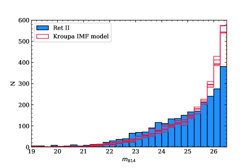
Figure 4.— Comparison between the observed F814W stellar luminosity function of Ret II (blue histogram) and a model drawn from a Kroupa (2001) IMF (red). Five realizations of the Kroupa model are displayed to provide a sense of the scatter associated with the random draws. Here we have assumed a binary fraction of $f_{b}=0.07$ (see §4.2), but different values produce similar results. The plotted model uses the binary mass ratio distribution for $0.4~{}{\rm\,M_{\odot}}<M<0.6~{}{\rm\,M_{\odot}}$, but the results for the $0.6~{}{\rm\,M_{\odot}}<M<0.8~{}{\rm\,M_{\odot}}$ mass ratio distribution are similar. Relative to the data, a Kroupa IMF produces too many faint stars ($m_{814}\gtrsim 25.75$) and too few stars at brighter magnitudes ($m_{814}\lesssim 25$).

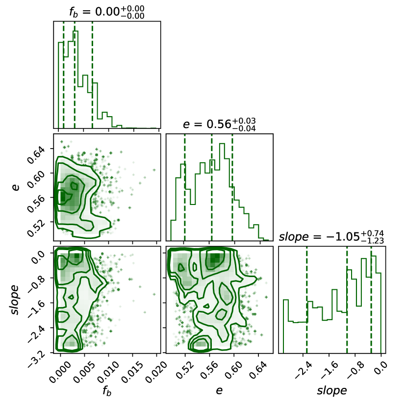
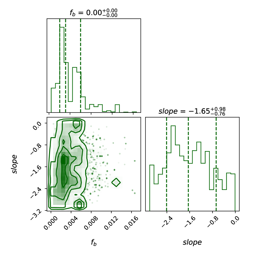
Figure 5.— Left panel: Posterior distributions of three parameters for a simulated dwarf galaxy with $f_{b}=0$, $R_{h}=6\farcm 3$, and $e=0.6$. The recovered binary fraction of $f_{b}=0.003^{+0.004}_{-0.002}$ and ellipticity of $e=0.56^{+0.04}_{-0.03}$ are in agreement with the input values. Right panel: Posterior distributions of two parameters of our model fitting a simulated dwarf with the same input parameters but the ellipticity held fixed. The recovered binary fraction is the same, but the uncertainties are smaller than when the ellipticity is included as a parameter in the MCMC fit.

4. Results

4.1. Tests with Mock Data

First, we test our method by carrying out MCMC fits on mock data sets (generated as described above) with known parameters. All mock data are constructed to match the sample size of the Ret II data set, and all MCMC simulations adopt top-hat priors for the binary fraction and power-law slope of the separation distribution with boundaries of $0\leq f_{b}\leq 1$ and $-2.0\leq\beta\leq-1.01$, respectively, and a Gaussian prior centered at $\epsilon=0.6$ with $\sigma=0.03$ for the ellipticity. Since our initial goal is to test the null hypothesis that the binary fraction is zero in Ret II, the first simulated dwarf contains no binaries ($f_{b}=0$). We then run an MCMC simulation to fit for the parameters of the model in this 3D parameter space and show the posterior distribution of each parameter in the left panel of Figure 5. The recovered posterior for the binary fraction is $f_{b}=0.003^{+0.004}_{-0.002}$ and the ellipticity is $e=0.56^{+0.04}_{-0.03}$. These values are consistent with the input values for the simulated dwarf, confirming that we can recover a zero binary fraction with confidence. The median derived value for the slope of the binary separation distribution is also consistent with the true value, but the posterior probability distribution is so broad that the constraint on this parameter is not useful.

We also explore holding the ellipticity of the galaxy fixed in the fit and using the MCMC procedure to determine only the binary parameters, since the ellipticity is already rather tightly constrained by the photometry. In this case, the recovered binary fraction is unchanged, at $f_{b}=0.003^{+0.003}_{-0.001}$, but the uncertainties are somewhat smaller, indicating that a fit with fewer parameters may be beneficial in determining more accurate binary properties. The results of this fit are displayed in the right panel of Figure 5. Fixing both the ellipticity and the slope of the separation distribution produces very similar results.

Finally, we investigated the impact of assuming an incorrect half-light radius. We constructed a simulated galaxy with a half-light radius of 5$\farcm$5, more than 2-$\sigma$ away from the true value, and then fit that data set with $R_{h}=6\farcm 3$ (and vice versa). Our results indicate that assuming a half-light radius offset from the true value by substantial amounts has a negligible effect on the recovered binary fraction. Extending these tests to $f_{b}>0$, we find that the fits generally recover the input binary fraction within the uncertainties regardless of which fit parameters are held fixed. Thus, although in our analysis below we do not know the intrinsic separation distribution for binaries in Ret II or the true geometry of the galaxy, we conclude that there is no evidence that our inferred binary fraction should be biased.

4.2. Fits to the Observed Ret II Data Set

Next, we move to performing the same analysis on the HST observations of Ret II, with results displayed in Figure 6. With a three parameter fit, the fraction of stars with a companion at separations between 0$\farcs$1 and 10″ is $f_{b}=0.007^{+0.008}_{-0.003}$. The slope of the power-law describing the binary separation distribution is unconstrained by the data, but is consistent with the value of $\beta=-1.6$ found for binary systems in the solar neighborhood (e.g., Chanamé & Gould, 2004; Lépine & Bongiorno, 2007; El-Badry & Rix, 2018; Tian et al., 2020)

If we instead impose $e=0.6$ and fit for the remaining two parameters, we recover an essentially identical posterior distribution of $f_{b}=0.007^{+0.007}_{-0.004}$. Finally, with both the ellipticity and the slope ($\beta=-1.6$) fixed, the derived binary fraction remains unchanged at $f_{b}=0.008^{+0.007}_{-0.005}$.

Since numerical simulations have shown that binaries with semi-major axis $\gtrsim 1$ pc are prone to disruption by tidal forces (Peñarrubia et al., 2016), we also repeat our MCMC simulations with a maximum angular separation of 5″ (0.75 pc) instead of 10″   We find that the inferred binary fraction does not depend significantly on the range of separations considered in the fit. The only choice in our analysis that has any impact on the fit results is the assumed minimum detectable separation between stars. Increasing the separation limit from 0$\farcs$1 to 0$\farcs$15 or 0$\farcs$2 raises the binary fraction to $f_{b}=0.009^{+0.006}_{-0.004}$ or $f_{b}=0.013^{+0.005}_{-0.006}$, respectively. However, we note that both of those values agree with the result for a minimum separation of 0$\farcs$1 within the uncertainties, so we do not regard these changes as significant.

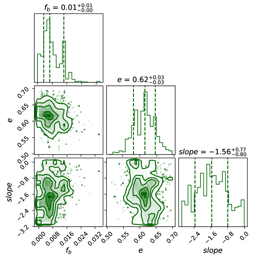
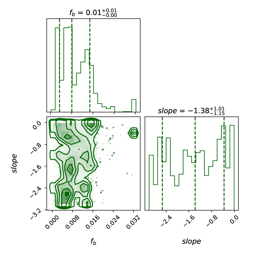
Figure 6.— Left panel: Posterior distributions for our four parameter model fitting the Ret II nearest neighbor separations, assuming a half-light radius of $R_{h}=6\farcm 3$. Right panel: Posterior distributions for our three parameter model fitting Ret II, assuming $R_{h}=6\farcm 3$ and fixing $e=0.6$. The recovered posterior distribution of $f_{b}=0.07^{+0.04}_{-0.03}$ is a statistically significant result compared to what we recovered for a simulated dwarf containing no binaries (see Figure 5).

4.3. IMF Constraints

To assess the IMF in Ret II quantitatively, we draw random samples of 2587 stellar masses according to IMF power-law indices ranging from $\alpha=1.01$ to $\alpha=2.0$ in steps of 0.01. (Here we are assuming that the IMF can be described by a single power law over the mass range probed by our data.) We repeat the random draws 100 times for each value of the IMF slope in order to improve the statistics, and convert all stellar masses into observed magnitudes in the F814W band using a PARSEC isochrone. For each set of model magnitudes, we use a 2-sample Kolmogorov-Smirnov test to calculate the probability $p$ that the observed magnitude distribution and the model are consistent with being drawn from the same probability distribution. There is some correlation between the assumed wide binary fraction and the IMF slope, but for the range of wide binary fractions allowed by the data the effect on $\alpha$ is small. We find that the magnitude distribution of stars in Ret II requires an IMF much shallower than the Salpeter (1955) value of $\alpha=2.35$ (see Fig. 7). For $f_{b}=0.01$, the maximum $p$-values occur at $1.01\leq\alpha\leq 1.15$, and the 84th percentile of the $p$-values (corresponding to a $1\sigma$ upper limit for a Gaussian distribution) is at least $p=0.05$ for $1.01\leq\alpha\leq{\color[rgb]{0,0,0}{1.42}}$. Increasing the binary fraction to larger values preserves the preference for $\alpha~{}{\color[rgb]{0,0,0}{\lesssim}}1.1$ and decreases the quality of the fit for steeper slopes. The differences between using the $0.4~{}{\rm\,M_{\odot}}<M<0.6~{}{\rm\,M_{\odot}}$ and $0.6~{}{\rm\,M_{\odot}}<M<0.8~{}{\rm\,M_{\odot}}$ binary mass ratio distributions (as described in § 3.2) are negligible. This result is consistent with the IMF slopes determined for the UFDs Canes Venatici II, Hercules, Leo IV, and Ursa Major I (all of which are somewhat more luminous than Ret II) by Geha et al. (2013) and Gennaro et al. (2018a). Gennaro et al. (2018a, b) obtained modestly steeper IMFs for the UFDs Boötes I and Coma Berenices, where Coma Ber is the closest of these galaxies to Ret II in luminosity (Muñoz et al., 2018) and metallicity (Kirby et al., 2013b).

5. Discussion and Implications

We have presented the first observational search for wide binary systems in a UFD via high angular resolution imaging. Our approach is based on the 2 point correlation function (e.g., Peñarrubia et al., 2016; Kervick et al., 2021), cast in the form of the nearest neighbor statistic. We find that the spatial distribution of stars in Ret II at small separations is consistent with a fraction of $0.007^{+0.008}_{-0.003}$ of Ret II stars possessing a companion in the separation range from 0$\farcs$1 ($3000$ AU) to 10″ ($3\times 10^{5}$ AU).

Combining the Gaia eDR3 wide binary catalog of El-Badry et al. (2021) with the Gaia Catalog of Nearby Stars (Gaia Collaboration et al., 2021b), we find that in the solar neighborhood, 0.3% of main sequence stars have a companion at a separation beyond 3000 AU that would be bright enough to observe in our Ret II data set. The wide binary fraction in Ret II is somewhat higher than, but consistent with, this value. The overall fraction of nearby stars that are in multiple systems is 44% (Raghavan et al., 2010), indicating that for the separation and mass ratio distributions in the Milky Way, only $\sim 1$% of binary systems have companions distant enough and bright enough to be detected at a distance of $\sim 30$ kpc. One might therefore suppose that the multiplicity rate in Ret II is also $\gtrsim 50$%, but the uncertainty on this estimate is quite large.

In recent work, Hwang et al. (2021) found that the wide binary fraction in the Milky Way declines by a factor of two from solar metallicity down to $\mathrm{[Fe/H]}=-1$. If that trend continues to lower metallicities, the wide binary fraction in Ret II would be expected to be $\sim 0.1$% or less, below our measured value (although only modestly inconsistent given the uncertainties). On the other hand, El-Badry & Rix (2019) derived a flat wide binary fraction with metallicity. Presuming that the primary difference between the star-forming conditions in Ret II in the early universe and those prevalent in the progenitors of the Milky Way stellar halo is metallicity, a lack of strong evolution in the wide binary fraction with metallicity is slightly more consistent with our results. However, more data in both the Milky Way and dwarf galaxies will be needed to draw strong conclusions.

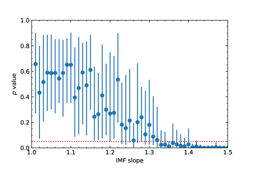
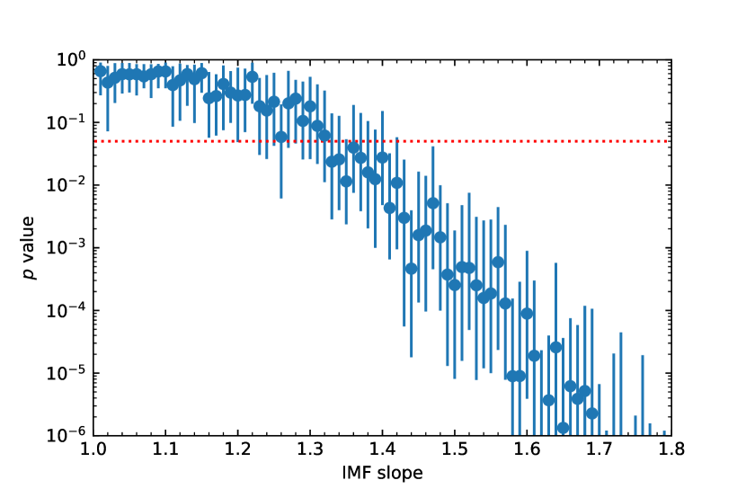
Figure 7.— Kolmogorov-Smirnov $p$-value from comparing the observed magnitude distribution in Ret II with models constructed with different IMF slopes. The left panel displays the results with a linear scale on the y axis to highlight the good fit obtained at $\alpha\lesssim{\color[rgb]{0,0,0}{1.15}}$, and the right panel uses a logarithmic scale to illustrate the behavior for steeper slopes. The error bars are plotted as the 16th and 84th percentiles of the distribution of $p$-values obtained for each slope. The red dotted line shows our limit of $p=0.05$ for a model to be considered a reasonable match to the data. The distribution of magnitudes in Ret II strongly prefers a shallow IMF slope of $\alpha\leq 1.4$ over the observed mass range of $0.34-0.78~{}{\rm\,M_{\odot}}$.

Although individual binary stars have been identified spectroscopically in UFDs (e.g., Frebel et al., 2010; Koposov et al., 2011; Koch et al., 2014; Venn et al., 2017; Li et al., 2018), relatively few constraints on the overall binary population in these galaxies are available. Using hierarchical Bayesian modeling of multi-epoch radial velocity measurements in Segue 1, Martinez et al. (2011) demonstrated that the galaxy must contain either a high fraction of binary stars or shorter mean binary periods than the Milky Way. However, they were only able to place a weak lower limit on the binary fraction of $f_{b}\sim 0.05$ at 68% confidence. Minor et al. (2019) used a similar method to investigate Ret II with a smaller spectroscopic sample, concluding that $f_{b}>0.5$ at 90% confidence. This result is not obviously inconsistent with our measurements, given the large difference in scales between the binaries we can detect and those whose kinematic signatures are observable.

The first photometric determination of the binary fraction in UFDs was by Geha et al. (2013), who modeled HST color-magnitude diagrams of Hercules and Leo IV to measure $f_{b}=0.47^{+0.16}_{-0.14}$ and $f_{b}=0.47^{+0.37}_{-0.17}$, respectively. More recently, Gennaro et al. (2018a) analyzed the entire HST data set of Brown et al. (2014) to study the IMF. They considered the binary fraction as a nuisance parameter, but found values spanning a very wide range, from $f_{b}=0.05^{+0.02}_{-0.05}$ for Canes Venatici II to $f_{b}=0.61\pm 0.14$ for Coma Berenices. On the other hand, employing deeper near-infrared HST imaging of Com Ber, Gennaro et al. (2018b) determined a smaller binary fraction of $0.25^{+0.08}_{-0.25}$.

Our technique for measuring the binary fraction is distinct from and complementary to the previous methods used in the literature. Other HST measurements relied on jointly fitting the colors and magnitudes of member stars to determine the IMF and the binary fraction simultaneously based on the photometric differences between single stars and unresolved binaries. Here, we use stellar positions to statistically identify spatially resolved binary stars. Encouragingly, the results from different techniques appear to be generally consistent, although as previously mentioned, the uncertainties at this stage are quite large. Spectroscopic follow-up of a larger sample of stars in Ret II and imaging searches for wide binaries in other nearby UFDs may shed additional light on this subject.

The steepness of the binary separation distribution and the distance of Ret II provide a relatively narrow range of separations over which wide Ret II binaries can be identified. We are therefore unable to determine whether the separation distribution in Ret II differs in any way from that observed in the Milky Way. The spectroscopic studies of Segue 1 and Ret II, which are sensitive to close binary systems, have suggested a shorter mean period distribution than in the Milky Way (Martinez et al., 2011; Minor et al., 2019). Similarly, Moe et al. (2019) infer shorter mean periods for metal-poor binary systems in the Milky Way. More specifically, they find that the close binary fraction is a strong inverse function of metallicity, while the wide binary fraction is independent of metallicity, so the dominant population of close binaries among metal-poor stars shifts the average period to smaller values. If the same result holds for UFDs, the influence of binary stars on their internal kinematics could be larger than would be estimated by assuming solar neighborhood binary properties.

The IMF in low-mass dwarf galaxies has generally been found to be shallower (more bottom-light) than that in the Milky Way (Wyse et al., 2002; Geha et al., 2013; Gennaro et al., 2018a, b). Our IMF measurement for Ret II is consistent with these results, with an IMF that is best described by a slope of $1.01\leq\alpha\leq 1.15$ when fit with a single power-law from $0.34~{}{\rm\,M_{\odot}}$ to $0.78~{}{\rm\,M_{\odot}}$. The UFDs therefore remain qualitatively consistent with a picture in which the IMF varies systematically with metallicity, from bottom-heavy IMFs for the most massive galaxies (e.g., van Dokkum & Conroy, 2010; Spiniello et al., 2012) to bottom-light IMFs for the least luminous dwarfs (however, see Gennaro et al. 2018a for possible complications of this model). If the bottom-light IMF for the surviving low-mass stars in Ret II can be extrapolated to much higher masses, there are significant implications for the population of supernovae the galaxy hosted at early times, and hence its chemical evolution (e.g., Jeon et al., 2021).

The noisiness of the likelihood function and the large uncertainties we obtain on the fraction of wide binaries suggest that the primary limitation of the Ret II data set is the sample size. The HST imaging already extends beyond the half-light radius of Ret II, so imaging over a wider field, as will be possible with, e.g., the Roman Space Telescope (Akeson et al., 2019) may only result in modest improvements. Larger numbers of stars can be obtained from deeper imaging in the near-infrared, either with HST (e.g., Gennaro et al., 2018b) or with the James Webb Space Telescope. Alternatively, it may be preferable to target dwarf galaxies containing larger numbers of stars. Most such systems are more distant, limiting the spatial resolution that can be obtained, but the recently-discovered UFDs Carina II and Hydrus I are each a factor of $\sim 2$ more luminous than Ret II and are located at comparable distances from the Milky Way (Koposov et al., 2018; Torrealba et al., 2018). Space-based imaging of these galaxies therefore may provide new insight into the binary star populations in UFDs. In parallel, spectroscopic observations of larger samples of UFD stars over a longer time baseline — the earliest UFD radial velocities are now $\sim 15$ years old — can tighten constraints on close binary systems, and a joint analysis of the spectroscopy and imaging together could improve measurements of the binary separation distribution in these extreme environments.

References

- Aaronson (1983) Aaronson, M. 1983, ApJ, 266, L11
- Abbott et al. (2018) Abbott, T. M. C., Abdalla, F. B., Allam, S., et al. 2018, ApJS, 239, 18
- Akeson et al. (2019) Akeson, R., Armus, L., Bachelet, E., et al. 2019, arXiv e-prints, arXiv:1902.05569
- Badenes et al. (2018) Badenes, C., Mazzola, C., Thompson, T. A., et al. 2018, ApJ, 854, 147
- Bechtol et al. (2015) Bechtol, K., Drlica-Wagner, A., Balbinot, E., et al. 2015, ApJ, 807, 50
- Belokurov et al. (2006) Belokurov, V., Zucker, D. B., Evans, N. W., et al. 2006, ApJ, 647, L111
- Bressan et al. (2012) Bressan, A., Marigo, P., Girardi, L., et al. 2012, MNRAS, 427, 127
- Brown et al. (2014) Brown, T. M., Tumlinson, J., Geha, M., et al. 2014, ApJ, 796, 91
- Brown et al. (2014) Brown, T. M., Tumlinson, J., Geha, M., et al. 2014, The Astrophysical Journal
- Burkert (2020) Burkert, A. 2020, ApJ, 904, 161
- Buttry et al. (2021) Buttry, R., Pace, A. B., Koposov, S. E., et al. 2021, arXiv e-prints, arXiv:2108.10867
- Calabrese & Spergel (2016) Calabrese, E., & Spergel, D. N. 2016, MNRAS, 460, 4397
- Chanamé & Gould (2004) Chanamé, J., & Gould, A. 2004, ApJ, 601, 289
- Chen et al. (2014) Chen, Y., Girardi, L., Bressan, A., et al. 2014, MNRAS, 444, 2525
- Chulkov (2021) Chulkov, D. 2021, MNRAS, 501, 769
- Drlica-Wagner et al. (2020) Drlica-Wagner, A., Bechtol, K., Mau, S., et al. 2020, ApJ, 893, 47
- El-Badry & Rix (2018) El-Badry, K., & Rix, H.-W. 2018, MNRAS, 480, 4884
- El-Badry & Rix (2019) —. 2019, MNRAS, 482, L139
- El-Badry et al. (2021) El-Badry, K., Rix, H.-W., & Heintz, T. M. 2021, MNRAS, arXiv:2101.05282 [astro-ph.SR]
- El-Badry et al. (2019) El-Badry, K., Rix, H.-W., Tian, H., Duchêne, G., & Moe, M. 2019, MNRAS, 489, 5822
- Ford et al. (2003) Ford, H. C., Clampin, M., Hartig, G. F., et al. 2003, Society of Photo-Optical Instrumentation Engineers (SPIE) Conference Series, Vol. 4854, Overview of the Advanced Camera for Surveys on-orbit performance, ed. J. C. Blades & O. H. W. Siegmund, 81
- Foreman-Mackey et al. (2013) Foreman-Mackey, D., Hogg, D. W., Lang, D., & Goodman, J. 2013, PASP, 125, 306
- Frebel et al. (2010) Frebel, A., Simon, J. D., Geha, M., & Willman, B. 2010, ApJ, 708, 560
- Fu et al. (2019) Fu, S. W., Simon, J. D., & Alarcón Jara, A. G. 2019, ApJ, 883, 11
- Gaia Collaboration et al. (2016) Gaia Collaboration, Prusti, T., de Bruijne, J. H. J., et al. 2016, A&A, 595, A1
- Gaia Collaboration et al. (2021a) Gaia Collaboration, Brown, A. G. A., Vallenari, A., et al. 2021a, A&A, 649, A1
- Gaia Collaboration et al. (2021b) Gaia Collaboration, Smart, R. L., Sarro, L. M., et al. 2021b, A&A, 649, A6
- Geha et al. (2009) Geha, M., Willman, B., Simon, J. D., et al. 2009, ApJ, 692, 1464
- Geha et al. (2013) Geha, M., Brown, T. M., Tumlinson, J., et al. 2013, ApJ, 771, 29
- Gennaro et al. (2018a) Gennaro, M., Tchernyshyov, K., Brown, T. M., et al. 2018a, ApJ, 855, 20
- Gennaro et al. (2018b) Gennaro, M., Geha, M., Tchernyshyov, K., et al. 2018b, ApJ, 863, 38
- Hayashi et al. (2021) Hayashi, K., Ferreira, E. G. M., & Jowett Chan, H. Y. 2021, arXiv e-prints, arXiv:2102.05300
- Hwang et al. (2021) Hwang, H.-C., Ting, Y.-S., Schlaufman, K. C., Zakamska, N. L., & Wyse, R. F. G. 2021, MNRAS, 501, 4329
- Jenkins et al. (2020) Jenkins, S., Li, T. S., Pace, A. B., et al. 2020, ApJ, in press, arXiv:2101.00013
- Jeon et al. (2021) Jeon, M., Besla, G., & Bromm, V. 2021, MNRAS, 506, 1850
- Ji et al. (2016) Ji, A. P., Frebel, A., Simon, J. D., & Geha, M. 2016, ApJ, 817, 41
- Kervick et al. (2021) Kervick, C., Walker, M. G., Peñarrubia, J., & Koposov, S. E. 2021, submitted to ApJ, arXiv:2107.07554
- Kirby et al. (2013a) Kirby, E. N., Boylan-Kolchin, M., Cohen, J. G., et al. 2013a, ApJ, 770, 16
- Kirby et al. (2013b) Kirby, E. N., Cohen, J. G., Guhathakurta, P., et al. 2013b, ApJ, 779, 102
- Kirby et al. (2017) Kirby, E. N., Cohen, J. G., Simon, J. D., et al. 2017, ApJ, 838, 83
- Kleyna et al. (2005) Kleyna, J. T., Wilkinson, M. I., Evans, N. W., & Gilmore, G. 2005, ApJ, 630, L141
- Koch et al. (2014) Koch, A., Hansen, T., Feltzing, S., & Wilkinson, M. I. 2014, ApJ, 780, 91
- Koposov et al. (2015) Koposov, S. E., Belokurov, V., Torrealba, G., & Evans, N. W. 2015, ApJ, 805, 130
- Koposov et al. (2011) Koposov, S. E., Gilmore, G., Walker, M. G., et al. 2011, ApJ, 736, 146
- Koposov et al. (2018) Koposov, S. E., Walker, M. G., Belokurov, V., et al. 2018, MNRAS, 479, 5343
- Kouwenhoven et al. (2009) Kouwenhoven, M. B. N., Brown, A. G. A., Goodwin, S. P., Portegies Zwart, S. F., & Kaper, L. 2009, A&A, 493, 979
- Kroupa (2001) Kroupa, P. 2001, Monthly Notices of the Royal Astronomical Society
- Lépine & Bongiorno (2007) Lépine, S., & Bongiorno, B. 2007, AJ, 133, 889
- Li et al. (2018) Li, T. S., Simon, J. D., Pace, A. B., et al. 2018, ApJ, 857, 145
- Marigo et al. (2017) Marigo, P., Girardi, L., Bressan, A., et al. 2017, ApJ, 835, 77
- Martinez et al. (2011) Martinez, G. D., Minor, Q. E., Bullock, J., et al. 2011, ApJ, 738, 55
- McConnachie & Côté (2010) McConnachie, A. W., & Côté, P. 2010, ApJ, 722, L209
- McGaugh & Wolf (2010) McGaugh, S. S., & Wolf, J. 2010, ApJ, 722, 248
- Minor et al. (2010) Minor, Q. E., Martinez, G., Bullock, J., Kaplinghat, M., & Trainor, R. 2010, ApJ, 721, 1142
- Minor et al. (2019) Minor, Q. E., Pace, A. B., Marshall, J. L., & Strigari, L. E. 2019, MNRAS, 487, 2961
- Moe et al. (2019) Moe, M., Kratter, K. M., & Badenes, C. 2019, ApJ, 875, 61
- Moskowitz & Walker (2020) Moskowitz, A. G., & Walker, M. G. 2020, ApJ, 892, 27
- Muñoz et al. (2018) Muñoz, R. R., Côté, P., Santana, F. A., et al. 2018, ApJ, 860, 66
- Mutlu-Pakdil et al. (2018) Mutlu-Pakdil, B., Sand, D. J., Carlin, J. L., et al. 2018, ApJ, 863, 25
- Nadler et al. (2021) Nadler, E. O., Drlica-Wagner, A., Bechtol, K., et al. 2021, Phys. Rev. Lett., 126, 091101
- Peñarrubia et al. (2016) Peñarrubia, J., Ludlow, A. D., Chanamé, J., & Walker, M. G. 2016, MNRAS, 461, L72
- Raghavan et al. (2010) Raghavan, D., McAlister, H. A., Henry, T. J., et al. 2010, The Astrophysical Journal Supplement Series, 1007.0414
- Sacchi et al. (2021) Sacchi, E., Richstein, H., Kallivayalil, N., et al. 2021, ApJ, 920, L19
- Safarzadeh & Loeb (2021) Safarzadeh, M., & Loeb, A. 2021, arXiv e-prints, arXiv:2104.13961
- Safarzadeh & Spergel (2020) Safarzadeh, M., & Spergel, D. N. 2020, ApJ, 893, 21
- Salpeter (1955) Salpeter, E. E. 1955, ApJ, 121, 161
- Schlafly & Finkbeiner (2011) Schlafly, E. F., & Finkbeiner, D. P. 2011, ApJ, 737, 103
- Simon (2019) Simon, J. D. 2019, ARA&A, 57, 375
- Simon & Geha (2007) Simon, J. D., & Geha, M. 2007, ApJ, 670, 313
- Simon et al. (2011) Simon, J. D., Geha, M., Minor, Q. E., et al. 2011, ApJ, 733, 46
- Simon et al. (2015) Simon, J. D., Drlica-Wagner, A., Li, T. S., et al. 2015, ApJ, 808, 95
- Simon et al. (2021) Simon, J. D., Brown, T. M., Drlica-Wagner, A., et al. 2021, ApJ, 908, 18
- Speagle (2020) Speagle, J. S. 2020, MNRAS, 493, 3132
- Spencer et al. (2018) Spencer, M. E., Mateo, M., Olszewski, E. W., et al. 2018, AJ, 156, 257
- Spiniello et al. (2012) Spiniello, C., Trager, S. C., Koopmans, L. V. E., & Chen, Y. P. 2012, ApJ, 753, L32
- Stetson (1987) Stetson, P. B. 1987, PASP, 99, 191
- Tian et al. (2020) Tian, H.-J., El-Badry, K., Rix, H.-W., & Gould, A. 2020, ApJS, 246, 4
- Torrealba et al. (2018) Torrealba, G., Belokurov, V., Koposov, S. E., et al. 2018, MNRAS, 475, 5085
- van Dokkum & Conroy (2010) van Dokkum, P. G., & Conroy, C. 2010, Nature, 468, 940
- Venn et al. (2017) Venn, K. A., Starkenburg, E., Malo, L., Martin, N., & Laevens, B. P. M. 2017, MNRAS, 466, 3741
- Willman et al. (2005) Willman, B., Dalcanton, J. J., Martinez-Delgado, D., et al. 2005, ApJ, 626, L85
- Wolf et al. (2010) Wolf, J., Martinez, G. D., Bullock, J. S., et al. 2010, MNRAS, 406, 1220
- Wyse et al. (2002) Wyse, R. F. G., Gilmore, G., Houdashelt, M. L., et al. 2002, New Astronomy, 7, 395
- Zucker et al. (2006) Zucker, D. B., Belokurov, V., Evans, N. W., et al. 2006, ApJ, 643, L103