Quantum effects in structural and elastic properties of graphite: Path-integral simulations

Abstract

Graphite, as a well-known carbon-based solid, is a paradigmatic example of the so-called van der Waals layered materials, which display a large anisotropy in their physical properties. Here we study quantum effects in structural and elastic properties of graphite by using path-integral molecular dynamics simulations in the temperature range from 50 to 1500 K. This method takes into account quantization and anharmonicity of vibrational modes in the material. Our results are compared with those found by using classical molecular dynamics simulations. We analyze the volume and in-plane area as functions of temperature and external stress. The quantum motion is essential to correctly describe the in-plane and out-of-plane thermal expansion. Quantum effects cause also changes in the elastic properties of graphite with respect to a classical model. At low temperature we find an appreciable decrease in the linear elastic constants, mainly in $C_{12}$ and $C_{44}$. Quantum corrections in stiffness constants can be in some cases even larger than 20%. The bulk modulus and Poisson’s ratio are reduced in a 4% and 19%, respectively, due to zero-point motion of the C atoms. These quantum effects in structural and elastic properties of graphite are nonnegligible up to temperatures higher than 300 K.

I Introduction

Over the last few decades, we have witnessed a large progress in the knowledge of carbon-based materials with $sp^{2}$ orbital hybridization, as fullerenes, carbon nanotubes, and graphene,Hone (2001); Hone et al. (2000); Geim and Novoselov (2007); Katsnelson (2007) which has progressively broadened the scope of this research field further than the traditionally known graphite. This classical material has in turn become a paradigmatic case of the nowadays called van der Waals materials, characterized by a layered structure, where the interactions between sheets are much weaker than those between atoms in each sheet.Frisenda et al. (2020) Among these materials one finds hexagonal boron nitride, transition-metal dichalcogenides, and III-VI compounds as InSe and GaS.Ajayan et al. (2016)

In addition to its common role in several areas as lubrication, batteries, and nuclear technology, graphite has had a renewed interest in recent years in connection with the discovery of graphene and the potential applications of this two-dimensional material. In particular, mechanical properties of graphite, including elastic constants, have been studied by using experimental and theoretical methods.Blakslee et al. (1970); Bosak et al. (2007); Nicklow et al. (1972); Boettger (1997); Jansen and Freeman (1987); Hasegawa and Nishidate (2004); Mounet and Marzari (2005); Michel and Verberck (2008); Savini et al. (2011) Nevertheless, a precise knowledge of these properties has been limited by the difficulty of obtaining high-quality single crystalline samples.Rollings et al. (2006); Zhou et al. (2005) Thus, although there is a general agreement on the values of the largest elastic stiffness constants (i.e., their relative uncertainty is a few percent), values of smaller elastic constants such as $C_{44}$ and $C_{13}$ are known with relatively large error bars. For $C_{13}$, for example, one finds in the literature values of 0(3) GPaBosak et al. (2007) and 15(5) GPa,Blakslee et al. (1970) derived from apparently reliable methods. This is in part due to the high anisotropy of graphite, which means that elastic stiffness constants related to in-plane deformations, as $C_{11}$ and $C_{12}$, are much larger than those related to deformations along the $z$-axis perpendicular to the basal plane.

Theoretical work has been carried out to study structural, elastic, and thermodynamic properties of graphite. Most of the calculations and simulations performed to analyze such properties of graphite (and solids in general) have considered atomic nuclei as classical particles. This means that their quantum zero-point motion is not taken into account in zero-temperature calculations, and their motion is assumed to be classical (i.e., follows Newton’s laws) in finite-temperature Monte Carlo or molecular dynamics (MD) simulations. The quantum delocalization of atomic nuclei becomes unimportant at high temperatures, but can lead to appreciable corrections in physical observables for $T$ lower than the Debye temperature of the material, $\Theta_{D}$.Kittel (1996) Throughout this paper we call nuclear quantum effects those caused by the quantum nature of atomic nuclei, which manifests itself in a spacial delocalization larger than that expected for a classical calculation (thermal motion).

Several research groups employed density-functional theory (DFT) calculations at $T=0$, and in some cases finite temperatures were considered by using a quantum quasiharmonic approximation (QHA) for the vibrational modes.Mounet and Marzari (2005); Sevik (2014); Mann et al. (2017) This approach is generally accepted to be sound at low temperature, but it can be inaccurate for layered materials at relatively high temperatures, as a consequence of an appreciable anharmonic coupling between out-of-plane and in-plane vibrational modes, which is not considered in a QHA. Various works based on classical molecular dynamics and Monte Carlo simulations of graphite have also appeared in the literature.Ghiringhelli et al. (2005); Tsai and Tu (2010); Colonna et al. (2011); Trevethan and Heggie (2016); Petersen and Gillette (2018); Korkut (2014); Dunn and Duffy (2011) For this layered material, frequencies of out-of-plane vibrational modes are lower than those of in-plane vibrations, and one can define two different Debye temperatures, one for the first set of modes ($\Theta_{D}^{\rm out}\sim$ 1000 K) and another for the second ($\Theta_{D}^{\rm in}\sim$ 2500 K).Krumhansl and Brooks (1953); Nihira and Iwata (2003) This means that nuclear quantum effects are expected to be appreciable at temperatures in the order of 300 K and even higher.

The difficulties associated to using classical simulations can be surmounted by employing simulation techniques which take account of nuclear quantum effects in an explicit way, as those based on Feynman path integrals.Gillan (1988); Ceperley (1995); Brito et al. (2015); Herrero and Ramírez (2016) This procedure is in principle equivalent to a quantization of the vibrational modes in the solid, with the advantage that anharmonicities are directly included in the path-integral simulation procedures. This kind of methods have been used to study properties of materials as diamond,Herrero and Ramírez (2000); Brito et al. (2020) silicon,Noya et al. (1996) boron nitride,Calvo and Magnin (2016); Brito et al. (2019) and graphene.Brito et al. (2015); Herrero and Ramírez (2016, 2019) We are not aware of any quantum atomistic simulation of graphite. An important point is the large anisotropy of this material, so that quantum effects can be quantitatively very different for properties along directions on the basal plane or perpendicular to it.

Here we employ the path-integral molecular dynamics (PIMD) method to study structural and elastic properties of graphite in a temperature range from 50 to 1500 K. The importance of nuclear quantum effects in the considered variables is assessed by comparing the results of quantum simulations with those obtained from classical MD simulations. We find that considering nuclear quantum motion is necessary for an adequate description of the in-plane thermal expansion. In general, quantum effects are nonnegligible in structural and elastic properties of graphite for temperatures even higher than 300 K. Particular attention is set on the temperature dependence of the linear elastic constants and bulk modulus of graphite. At low temperature, quantum corrections in elastic stiffness constants may be higher than 20%, whereas the Poisson’s ratio and bulk modulus are appreciably reduced.

The paper is organized as follows. In Sec. II we describe the computational methods employed in the simulations. In Sec. III we discuss the phonon dispersion bands and the calculation of elastic constants at $T=0$. Results for the internal energy of graphite are presented in Sec. IV. In Sec. V we show results for the volume and the in-plane area, and the thermal expansion is presented in Sec. VI. Data of the elastic constants and bulk modulus at finite temperatures are given and discussed in Secs. VII and VIII. Finally, we summarize the main results in Sec. IX.

II Computational Method

In this paper we study the influence of nuclear quantum effects on structural and elastic properties of graphite. This means that we consider quantum delocalization of atomic nuclei, and analyze its influence on physical observables of the material. This requires, on one side, the definition of a reliable potential to describe the interatomic interactions in the solid. This potential is usually derived from ab-initio methods (e.g., DFT), tight-binding-like Hamiltonians, or effective interactions. This provides one with a Born-Oppenheimer surface for motion of the atomic nuclei. On the other side, we need a method to take into account the quantum dynamics (or quantum delocalization) in the many-body configuration space of atomic coordinates with the selected interatomic interactions. This means that we have to base our finite-temperature calculations on quantum statistical physics, in contrast to the more usually employed classical statistical physics to perform Monte Carlo or molecular dynamics simulations.

Thus, we employ PIMD simulations to study equilibrium properties of graphite as a function of temperature and pressure. The PIMD method rests on the Feynman path-integral formulation of statistical mechanics,Feynman (1972) which turns out to be a suitable nonperturbative procedure to study many-body quantum systems at finite temperatures. In the implementation of this method, each quantum particle (here, atomic nucleus) is described as a set of $N_{\rm Tr}$ (Trotter number) beads, which act as classical particles building a ring polymer.Gillan (1988); Ceperley (1995) In this way, one has a classical isomorph displaying an unreal dynamics, as it does not represent the true dynamics of the actual quantum particles. This isomorph is, however, practical for an efficient sampling of the configuration space, thus giving accurate values for time-independent variables of the quantum system. Details on this simulation technique can be found in Refs. Gillan, 1988; Ceperley, 1995; Herrero and Ramírez, 2014; Cazorla and Boronat, 2017.

Interatomic interactions between C atoms are described here through a long-range bond order potential, the so-called LCBOPII, mainly employed earlier to perform classical simulations of carbon-based systems.Los et al. (2005) Notably, it has been used to study the phase diagram of carbon, including graphite, diamond, and the liquid, and displayed its precision by yielding rather accurately the graphite-diamond transition line.Ghiringhelli et al. (2005) More recently, this effective potential has been also found to accurately describe various properties of graphene.Fasolino et al. (2007); Los et al. (2016); Zakharchenko et al. (2009); Politano et al. (2012); Ramírez and Herrero (2017)

The LCBOPII potential was also employed in last years to perform PIMD simulations, providing a quantification of nuclear quantum effects in monolayer and bilayer graphene from a comparison with results of classical simulations.Herrero and Ramírez (2016, 2018) In this paper about graphite, as in earlier simulations of graphene,Ramírez et al. (2016); Herrero and Ramírez (2016); Ramírez and Herrero (2017) the original parameterization of the LCBOPII potential has been slightly modified to increase the zero-temperature bending constant $\kappa$ of the graphene layers from 1.1 eV to 1.49 eV, closer to experimental data.Lambin (2014); Tisi (2017) The interlayer interaction was fitted to the results of quantum Monte Carlo calculations,Spanu et al. (2009) to yield a binding energy of 50 meV/atom for graphite.Zakharchenko et al. (2010)

For the calculations presented here, we have employed both the isothermal-isobaric ($NPT$) and isothermal-isochoric ($NVT$) ensembles. For the $NVT$ simulations we used cell parameters obtained from equilibrium $NPT$ simulations at the same temperature. We have used effective algorithms for the PIMD simulations, as those presented in the literature.Tuckerman et al. (1992); Tuckerman and Hughes (1998); Martyna et al. (1999) In particular, we have employed staging coordinates to define the bead positions in the classical isomorph, and in order to keep a constant $T$ we have introduced chains of four Nosé-Hoover thermostats connected to each staging coordinate. In $NPT$ simulations, another chain of four thermostats was coupled to the barostat to give the equilibrium volume fluctuations for the considered external stress.Tuckerman (2010); Herrero and Ramírez (2014). The equations of motion have been integrated by using the reversible reference system propagator algorithm (RESPA), which allows to consider different time steps for the integration of the slow and fast degrees of freedom.Martyna et al. (1996) The time step corresponding to the interatomic forces was $\Delta t$ = 1 fs, which is adequate for the C atomic mass and the range of temperatures considered here. More details on this type of PIMD simulations are given elsewhere.Tuckerman and Hughes (1998); Herrero et al. (2006); Herrero and Ramírez (2011)

We considered orthorhombic simulation cells of graphite with $N$ = 960 atoms and similar side lengths in the in-plane $x$ and $y$ directions ($L_{x}\approx L_{y}$). These cells included four carbon sheets in AB stacking, each with $n$ = 240 atoms. Periodic boundary conditions were assumed. To check the convergence of our results, some simulations were carried out for larger simulation cells with $n$ = 960 atoms. As the size $n$ is increased, there appear vibrational modes with longer wavelength $\lambda$. In fact, one has an effective wavelength cutoff $\lambda_{\rm max}\approx L$, where $L=(L_{x}L_{y})^{1/2}$, which translates into a wavevector cutoff $k_{\rm min}\approx 2\pi/L$, with $k=|{\bf k}|$. The results obtained using $n$ = 240 and 960 atoms/layer for the energy, in-plane area, and interatomic distances coincide within the statistical error bars of our simulations. For example, for the energy and mean interatomic distance, differences are less than $6\times 10^{-4}$ eV/atom and $4\times 10^{-5}$ Å, respectively.

Sampling of the configuration space was performed in the temperature range between 50 K and 1500 K. The Trotter number $N_{\rm Tr}$ (number of beads in the ring polymers) varies with the temperature as $N_{\rm Tr}=6000~{}{\rm K}/T$, which gives a roughly constant accuracy of the PIMD results for different temperatures.Herrero et al. (2006); Herrero and Ramírez (2011); Ramírez et al. (2012) A typical simulation run in the $NVT$ or $NPT$ ensembles consisted of $2\times 10^{5}$ PIMD steps for system equilibration and $8\times 10^{6}$ steps for calculation of average variables. For comparison with the results of our quantum PIMD simulations, we have also carried out classical molecular dynamics simulations with the same interatomic potential. In our context, these classical simulations correspond to a Trotter number $N_{\rm Tr}=1$.

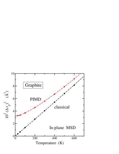
Figure 1: In-plane mean-square displacement, $(\Delta r_{p})^{2}=(\Delta x)^{2}+(\Delta y)^{2}$, of carbon atoms in graphite, as derived from classical MD (circles) and quantum PIMD simulations (squares) at various temperatures. Error bars are less than the symbol size.

In Fig. 1 we present the mean-square displacement (MSD) of carbon atoms in the $(x,y)$ layer plane, $(\Delta r_{p})^{2}=(\Delta x)^{2}+(\Delta y)^{2}$, at several temperatures and zero external pressure. Solid circles represent data points obtained from classical MD simulations, whereas squares indicate results of PIMD simulations. The classical results converge to zero in the low-temperature limit, as expected in classical physics, while the quantum data converge at low $T$ to $(\Delta r_{p})^{2}=3.4\times 10^{-3}$ Ų (in-plane zero-point delocalization). The difference between classical and quantum results decreases as temperature is raised, but is clearly appreciable in the whole temperature range displayed in Fig. 1. An even larger quantum delocalization occurs for the out-of-plane $z$-direction, which has been studied in detail for graphene in Ref. Herrero and Ramírez, 2016. Such atomic quantum delocalization (in-plane and out-of-plane) causes changes in the properties of the material, especially in the presence of anharmonicities in the lattice vibrations, as the atomic motion ”explores” larger regions of the configuration space, as compared to classical simulations.

The elastic stiffness constants at $T=0$ have been calculated from the phonon dispersion bands and cell distortions as explained in Sec. III. Relations between the elastic stiffness constants $C_{ij}$ and compliance constants $S_{ij}$ for hexagonal crystals, as well as their definitions as functions of the strain and stress components, $e_{ij}$ and $\tau_{ij}$, are given in the literatureMarsden et al. (2018); Li and Thompson (1990); Rabiei et al. (2020). We use the standard notation for strain components, with $e_{ij}=\epsilon_{ij}$ for $i=j$, and $e_{ij}=2\epsilon_{ij}$ for $i\neq j$ .Ashcroft and Mermin (1976); Marsden et al. (2018)

At finite temperatures, we have also obtained the elastic constants of graphite in two different ways. The first way consists in applying a certain component of the stress tensor in isothermal-isobaric simulations, and obtaining the associated elastic constants from the resulting strain. Thus, for example, for $\tau_{xx}\neq 0$ and $\tau_{ij}=0$ for the other components we can calculate $S_{11}$, $S_{12}$, and $S_{13}$. Then, from the obtained compliance constants we calculate the stiffness constants $C_{ij}$ using the relations corresponding to hexagonal crystals.Marsden et al. (2018); Li and Thompson (1990); Rabiei et al. (2020)

In the second way, we take as a reference for each temperature and kind of simulation (classical MD or PIMD) the simulation cell parameters obtained from equilibrium isothermal-isobaric simulations at that temperature. Then, we carry out $NVT$ simulations for cells strained a certain amount respect the equilibrium one. For example, for $e_{zz}\neq 0$ and $e_{ij}=0$ for the other components of the strain tensor, we obtain a stress tensor $\{\tau_{ij}\}$ from which we calculate the stiffness constants $C_{13}$ and $C_{33}$. Comparing the results of both methods provides us with a consistency check for our calculations.

III Phonon dispersion bands and elastic constants at $T=0$

The evaluation of the elastic stiffness constants, $C_{ij},$ of graphite with the LCBOPII potential model in the classical $T\rightarrow 0$ limit provides us with a useful reference for the subsequent analysis of temperature and nuclear quantum effects. Two alternative methods have been employed to derive $C_{ij}$ in this limit, namely the analysis of the harmonic dispersion relation of acoustic phonons, and the calculation of the elastic energy associated to some selected strain tensors, $\{e_{ij}\}$.

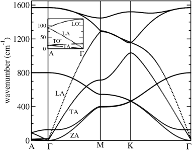
Figure 2: Phonon dispersion bands of graphite as derived from the LCBOPII potential model in a harmonic approximation. The labels LA, TA, and ZA refer to the acoustic bands employed in the calculation of the elastic stiffness constants. The inset amplifies the low-energy acoustic bands along the $\Gamma-A$ direction.

The phonon bands of graphite derived from the LCBOPII potential employed here are displayed in Fig. 2. These bands were obtained by diagonalization of the dynamical matrix along selected symmetry directions in reciprocal space. Interatomic force constants were derived by numerical differentiation of the forces using atom displacements of $1.5\times 10^{-3}$ Å with respect to the equilibrium positions. The phonon dispersion in Fig. 2 is similar to those obtained from other empirical potentials and DFT calculations.Wirtz and Rubio (2004) In Table I we present frequencies of optical modes at the $\Gamma$ point and acoustic modes at the high-symmetry points $M$, $K$, $A$ in $k$-space, derived from DFT calculations in the local-density approximation (LDA) and generalized-gradient approximation (GGA),Wirtz and Rubio (2004) as well as those obtained with the LCBOPII interatomic potential.

Table 1: Phonon frequencies (in cm^-1) at high-symmetry points in $k$-space, obtained in Ref. Wirtz and Rubio, 2004 from LDA and GGA-DFT calculations, along with those found for the LCBOPII interatomic potential employed here.

		LDA	GGA	LCBOPII
$\Gamma$	LO/TO	1597	1569	1570
	ZO	893	884	901
	TO’	43	—	21
	LO’	120	—	128
$M$	LA	1346	1338	1266
	TA	626	634	714
	ZA	472	476	396
$K$	LA/LO	1238	1221	1158
	ZA/ZO	535	539	465
	TA	1002	1004	1035
$A$	LA/LO’	85	—	90
	TA/TO’	30	—	14

The sound velocities for the three acoustic bands (LA, TA, and ZA) along the direction $\Gamma\mathrm{M}$, with wavevectors $(k_{x},0,0)$, correspond to the slopes $\left(\partial\omega/\partial k_{x}\right)_{\varGamma}$. For the hexagonal symmetry of graphite, these velocities are related to the elastic stiffness constants as follows:Newnham (2005)

$$\omega_{\rm LA}=\left(\frac{C_{11}}{\rho}\right)^{1/2}k_{x}\>,$$ (1)

$$\omega_{\rm TA}=\left(\frac{C_{11}-C_{12}}{2\rho}\right)^{1/2}k_{x}\>,$$ (2)

$$\omega_{\rm ZA}=\left(\frac{C_{44}}{\rho}\right)^{1/2}k_{x}\>,$$ (3)

where $\rho$ is the density of graphite. Along the $\Gamma\mathrm{A}$ direction, $(0,0,k_{z})$, the sound velocities of the LA and the twofold degenerate TA branches are given by,Newnham (2005)

$$\omega_{\rm LA}=\left(\frac{C_{33}}{\rho}\right)^{1/2}k_{z}\>,$$ (4)

$$\omega_{\rm TA}=\left(\frac{C_{44}}{\rho}\right)^{1/2}k_{z}\>.$$ (5)

The interatomic potential LCBOPII was employed earlier to obtain the phonon dispersion bands of graphene.Karssemeijer and Fasolino (2011) We note that the version of the potential used in that work was slightly different than that employed here, which is more realistic to describe the bending of the graphene sheets,Tisi (2017); Ramírez et al. (2016) as mentioned above in Sec. II.

Our second approach to determine $C_{ij}$ at $T=0$ consists in calculating the elastic energy, $E_{\rm elas}$, for small strains $e_{ij}$, which can be expressed as

$$\frac{E_{elas}}{V_{0}}=\frac{E-E_{0}}{V_{0}}=\frac{1}{2}\sum_{i=1}^{6}\sum_{j=1}^{6}C_{ij}e_{i}e_{j}\>,$$ (6)

where $E_{0}$ and $V_{0}$ are the energy and volume of the equilibrium configuration in the absence of strain (see below). We use the Voigt notation, where the components of the strain tensor are labeled as

$$\left\{e_{i},i=1,\ldots 6\right\}=\left\{e_{xx},e_{yy},e_{zz},e_{yz},e_{xz},e_{xy}\right\}\>.$$ (7)

Table 2: Definition of the six different cell strains employed to calculate the elastic energy and the classical value of the elastic stiffness constants at $T=0$. The isotropic bulk modulus, $B_{iso}$, is defined in Eq. (18).

strain	components, $e_{ij}\neq 0$	$E_{elas}/V_{0}$
1	$e_{xx}=e_{yy}=e$	$(C_{11}+C_{12})e^{2}$
2	$e_{xx}=-e_{yy}=e$	$(C_{11}-C_{12})e^{2}$
3	$e_{zz}=e$	$\frac{1}{2}C_{33}e^{2}$
4	$e_{xz}=e_{zx}=e$	$2C_{44}e^{2}$
5	$e_{xx}=e_{yy}=e_{zz}=e$	$\frac{9}{2}B_{iso}e^{2}$
6	$e_{xx}=e_{yy}=-\frac{e}{3},\>e_{zz}=\frac{2e}{3}$	$\frac{1}{9}(C_{11}+C_{12}+2C_{33}-4C_{13})e^{2}$

The elastic energy corresponding to six different strain tensors, employed in the evaluation of $C_{ij}$, is summarized in Table II. The tensor components are defined with the help of a dimensionless constant $e$. The elastic stiffness constants were obtained by quadratic fits of the function $E_{elas}/V_{0}$ for strains defined in the region $\left|e\right|\leq 2\times 10^{-3}$. One important aspect in the calculation of the elastic energy is that, whenever the solid lattice is subjected to a uniform strain, the atoms will rearrange themselves in the distorted lattice to minimize the elastic energy.Feynman et al. (1977); Stadler et al. (1996); Zhou and Huang (2008) This aspect is especially important in the case of strain 2 in Table II, where upon a uniform distortion of the lattice, one finds that the elastic energy is reduced by a 13% when internal relaxation of atomic positions in the distorted lattice is allowed. Only when this atomic relaxation is included, the elastic constants calculated by the elastic-energy method and the acoustic phonon dispersion agree with each other.Stadler et al. (1996) Our results for the classical $T\rightarrow 0$ limit of the elastic stiffness constants of graphite are summarized in Table III, along with also finite-temperature values which will be discussed below. The error bars in the classical zero-temperature values were derived from the differences encountered between both methods employed here, except for $C_{13}$, where the error bar corresponds to the results obtained with strains 5 and 6.

Table 3: Elastic stiffness constants, bulk modulus, and Poisson’s ratio of graphite, derived from classical and quantum simulations at $T$ = 0, 300 and 750 K. Data for $C_{ij}$ and $B$ are in GPa. We give in parenthesis the statistical error in the last digit.

	$T=0$		$T=300$ K		$T=750$ K
	class.	quantum	class.	quantum	class.	quantum
$C_{11}$	1007.7(5)	992(1)	969(1)	960(2)	917(2)	910(2)
$C_{12}$	216.3(3)	174(1)	175(1)	162(2)	134(1)	131(2)
$C_{13}$	1.05(4)	1.0(1)	3.4(1)	3.4(1)	5.7(1)	5.7(1)
$C_{33}$	37.1(1)	35.9(1)	34.6(1)	33.9(1)	31.6(1)	31.2(1)
$C_{44}$	1.03(2)	0.74(1)	0.61(1)	0.57(1)	0.42(2)	0.41(2)
$B$	35.1(1)	33.8(1)	33.0(1)	32.3(1)	30.4(1)	30.0(1)
$\nu$	0.215	0.175	0.181	0.169	0.146	0.144

IV Energy

In this section we present the internal energy of unstressed graphite, obtained from PIMD simulations in the isothermal-isobaric ensemble at various temperatures. This kind of simulations yield separately the kinetic and potential energy of the system,Herrero and Ramírez (2014); Ramírez and Herrero (2011) which allows us to analyze anharmonicities in the solid by comparing both energies. For given temperature and external stress, we express the internal energy as $E=E_{0}+E_{\rm pot}+E_{\rm kin}$, where $E_{\rm pot}$ and $E_{\rm kin}$ are the kinetic and potential energy, and $E_{0}$ is the energy of the classical model at $T=0$, i.e., the minimum-energy configuration of the considered LCBOPII potential, with totally planar sheets and no atomic quantum delocalization.

In the classical minimum, the energy of graphite decreases by 50 meV/atom with respect to an isolated graphene monolayer. This stabilization energy, associated to layer interactions, is in line with that found from classical Monte Carlo simulations of bilayer graphene using the LCBOPII potentialZakharchenko et al. (2010) (25 meV/atom, since in this case each graphene layer has only one neighboring layer). The interlayer binding energies obtained from various ab-initio calculations for the AB stacking of graphite display a rather large dispersion, with most data between 20 and 80 meV/atom.Hasegawa and Nishidate (2004); Hasegawa et al. (2007); Mostaani et al. (2015) Experimental values at room temperature lie between 35 and 52 meV/atom.Hasegawa and Nishidate (2004)

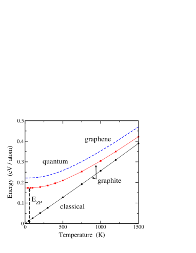
Figure 3: Internal energy of unstressed graphite as a function of temperature, obtained from PIMD (squares) and classical MD simulations (circles). Solid lines are guides to the eye. Error bars are less than the symbol size. A vertical dashed arrow indicates the zero-point energy, $E_{\rm ZP}$ = 173 meV/atom. A dashed line shows the internal energy of monolayer graphene, as derived from PIMD simulations.

In Fig. 3 we display the temperature dependence of the internal energy per atom, $E-E_{0}$, as derived from our PIMD simulations of unstressed graphite (solid squares). For comparison, we also show the internal energy obtained from classical MD simulations (circles). In the quantum case, $E-E_{0}$ converges in the low-$T$ limit to a zero-point energy $E_{\rm ZP}$ = 173 meV/atom. This value is slightly higher than that corresponding to a graphene monolayerHerrero and Ramírez (2016) ($E_{\rm ZP}=171$ meV/atom), which indicates that most of the zero-point energy is due to high-frequency in-plane vibrational modes, which are not appreciably changed by the interaction between layers.

In the quantum model, the internal energy follows at low temperature ($T<200$ K) a dependence $E-E_{0}\sim T^{3}$, which is consistent with the known dependence $c_{p}\sim T^{2}$ for the specific heat of graphite in this temperature region.Desorbo and Nichols (1958); Herrero and Ramírez (2020a) The classical model yields at low $T$ a dependence $E-E_{0}\sim T$, as expected from the equipartition principle in classical statistical mechanics for harmonic lattice vibrations, which gives the Dulong-Petit law: $c_{p}=3Nk_{B}$ irrespective of $T$. At high $T$ we find from the classical simulations slight deviations from this law, due to anharmonicity of the vibrational modes. The energy data found from PIMD simulations converge to those of classical MD simulations as temperature is raised. However at $T=1000$ K we still observe a significant difference between quantum and classical results, close to 50 meV/atom.

The dashed line in Fig. 3 represents the internal energy per atom for a graphene monolayer, as derived from PIMD simulations. This line is shifted upwards by $\Delta E=$ 48 meV/atom with respect to the quantum data of graphite, which is the effective interlayer interaction. This value is slightly lower than that found in the classical calculation at $T=0$ ($\Delta E=$ 50 meV/atom), due to the larger zero-point energy per atom in graphite.

As indicated above, an overall quantification of the anharmonicity of vibrational modes in graphite can be obtained by comparing the kinetic and potential energy yielded by PIMD simulations. For strictly harmonic vibrations, one has $E_{\rm kin}=E_{\rm pot}$ (virial theorem), so departure from pure harmonicity can be assessed in view of deviations from unity of the ratio $E_{\rm kin}/E_{\rm pot}$. At low $T$, we find for graphite a ratio $E_{\rm kin}/E_{\rm pot}=1.02$. From earlier analysis of anharmonicity in solids, on the basis of quasiharmonic approximations and perturbation theory, it is known that for small $T$, changes in the vibrational energy with respect to a harmonic approach are essentially due to the kinetic-energy contribution. Indeed, for a perturbed harmonic oscillator with an energy perturbation proportional to $r^{3}$ or $r^{4}$ at $T=0$ (here $r$ is any coordinate in the problem), the first-order change in the energy is due to a variation of $E_{\rm kin}$, and $E_{\rm pot}$ keeps changeless as in the unperturbed oscillator.Herrero and Ramírez (1995); Landau and Lifshitz (1965)

V Structural variables

V.1 Crystal volume

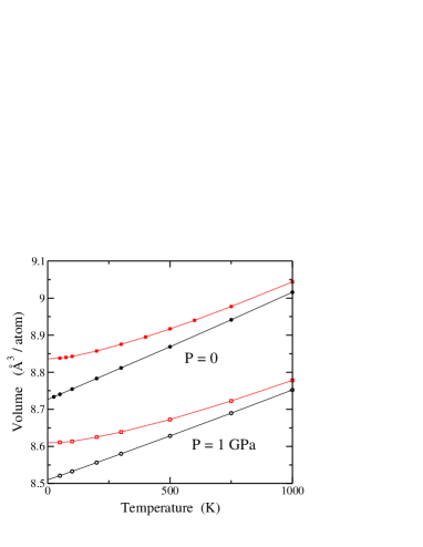
Figure 4: Temperature dependence of the crystal volume of graphite, as derived from PIMD (squares) and classical MD (circles) simulations for $P=0$ (solid symbols) and a hydrostatic pressure $P=1$ GPa (open symbols). Error bars are smaller than the symbol size.

In Fig. 4 we present the volume per atom as a function of temperature, as derived from classical MD (circles) and PIMD simulations (squares) in the $NPT$ ensemble for zero external stress (solid symbols) and a hydrostatic pressure $P=1$ GPa (open symbols). As is usual in Thermodynamics, and in the definition of the bulk modulus considered below, a compressive pressure is positive. In the stress-tensor notation employed in elasticity this corresponds to $\tau_{xx}=\tau_{yy}=\tau_{zz}=-1$ GPa, and $\tau_{\alpha\beta}=0$ for $\alpha\neq\beta$.

We comment first the results for the unstressed material. The data derived from classical simulations display a temperature dependence of the volume close to linear, with a positive slope $dV/dT$ slowly increasing for rising $T$. These data converge at low temperature to $V_{0}=8.727$ Å³/atom, which corresponds to the minimum-energy volume. For comparison, we mention that earlier theoretical work based mainly on DFT calculations gave values for $V_{0}$ between 8.61 and 8.94 Å³/atom.Jansen and Freeman (1987); Schabel and Martins (1992); Furthmuller et al. (1994); Boettger (1997) The equilibrium volume obtained from PIMD simulations at each temperature is larger than the classical result, and converges to 8.837 Å³/atom for $T\to 0$. This represents a zero-point volume expansion of 1.3% with respect to the classical minimum. At high temperature the quantum and classical data converge one to the other. Our results are not far from the volume obtained for graphite at ambient conditions from x-ray diffraction experiments: 8.78 and 8.80 Å³/atom in Refs. Hanfland et al., 1989 and Zhao and Spain, 1989, respectively.

At low temperature ($T\to 0$) the interlayer distance, $c$, increases from the classical limit by a 0.4%, and the linear expansion in the sheet plane ($x$ and $y$ directions) amounts also to a 0.4%. The zero-point expansion of a crystal is controlled by the anharmonicity of the lattice vibrations. In terms of a QHA, this expansion depends on each phonon through the product of its zero-point energy and the corresponding Grüneisen parameter.Ashcroft and Mermin (1976); Debernardi and Cardona (1996); Mounet and Marzari (2005); Herrero and Ramírez (2020b) Given that the main contributions to the in-plane and out-of-plane expansions are dominated by phonons with different polarization, it seems accidental that the relative quantum effects in directions $x$ and $z$ coincide, in spite of the large anisotropy of the material. This anisotropy is, however, clearly observable in the thermal expansion at finite temperatures (see Sec. VI).

For graphite under a hydrostatic pressure $P=1$ GPa, we obtain classical and quantum results similar to those found for the unstressed material, with the following differences. First, the volume is reduced, but this reduction is much less in the $(x,y)$ plane than in the out-of-plane $z$-direction, which corresponds to the different magnitudes of the elastic constants governing the compressibility in different crystal directions (see below). Second, the zero-point volume expansion is reduced with respect to that found for unstressed graphite. For $P=1$ GPa we find $\Delta V$ = 0.099 ų/atom for $T\to 0$ vs an expansion of 0.110 ų/atom for $P=0$. Third, the thermal dilation decreases under an applied hydrostatic pressure. In the temperature range from $T$ = 0 to 1000 K, we find from the PIMD data an expansion of 0.169 and 0.207 ų/atom for the stressed and unstressed material, respectively.

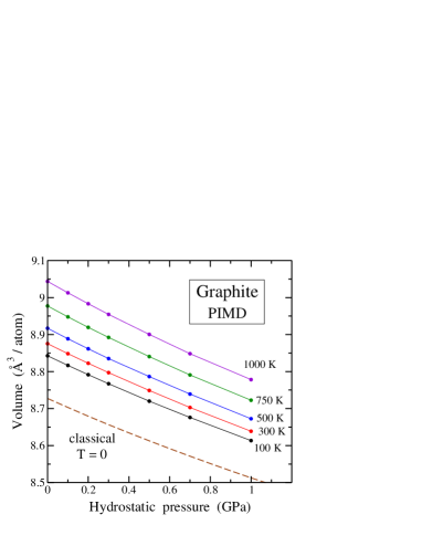
Figure 5: Volume of graphite as a function of hydrostatic pressure at various temperatures, as derived from PIMD simulations. From top to bottom, $T$ = 1000, 750, 500, 300, and 100 K. Solid lines are guides to the eye. A dashed line represents the pressure dependence of the classical volume at $T=0$.

The dependence of crystal volume on hydrostatic pressure is displayed in Fig. 5 for several temperatures. Symbols are data points derived from PIMD simulations and solid lines are guides to the eye. The dashed line indicates the pressure dependence of $V$ for the classical model at $T=0$. For each pressure $P$, this corresponds to the minimum of the enthalpy $H=E-PV$. Note the important difference between this classical result at $T=0$ and the quantum result at $T=100$ K (more than 0.1 Å³/atom), due to the low-temperature crystal expansion for the quantum model, as shown in Fig. 4. The solid lines in Fig. 5 seem at first sight rather parallel, but differences between their slopes (in particular at $P=0$) indicate changes in the bulk modulus of the material (see below). The volume differences between these isotherms become smaller as the hydrostatic pressure is increased. Thus, the difference between the quantum result at 100 K and the classical minimum is reduced by a 13% from $P$ = 0 to 1 GPa.

Volume changes under a hydrostatic pressure are related to the bulk modulus $B$, as discussed in Sec. VIII. From the classical data at $T=0$, we have $dV/dP=-0.246$ Å³/(atom GPa) in the limit $P\to 0$, whereas at $T$ = 1000 K, our PIMD simulations yield $dV/dP=-0.313$ Å³/(atom GPa).

The strain components $e_{xx}$ and $e_{zz}$ for a hydrostatic pressure $P$ can be obtained from the elastic compliance constants $S_{ij}$ asMarsden et al. (2018); Rabiei et al. (2020)

$$\frac{e_{xx}}{e_{zz}}=\frac{S_{11}+S_{12}+S_{13}}{2S_{13}+S_{33}}\;.$$ (8)

At room temperature ($T=300$ K) we find from our PIMD simulations $e_{xx}/e_{zz}$ = 0.027. At 1000 K this ratio decreases to 0.023.

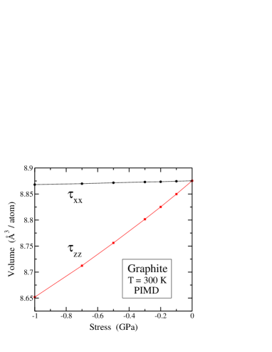
Figure 6: Volume of graphite as a function of uniaxial stress along the $x$ and $z$ directions of the orthorhombic simulation cell at $T$ = 300 K. $\tau_{xx}$ and $\tau_{zz}$ indicate the nonvanishing components of the stress tensor in each case. Symbols represent results of PIMD simulations, with error bars less than the symbol size. Lines are guides to the eye.

For the calculation of elastic constants at finite temperatures presented in Sec. VII, we have carried out simulations of graphite under various kinds of stress, given by the different components of the tensor $\{\tau_{ij}\}$, as explained in Sec. II. In Fig. 6 we present the dependence of the crystal volume on uniaxial stress along the $x$ and $z$ directions at $T$ = 300 K, as derived from PIMD simulations. These uniaxial stresses correspond to nonvanishing components of the stress tensor $\tau_{xx}$ and $\tau_{zz}$, respectively. The volume change in the second case is much larger than in the former, due to the higher compressibility in the $z$ direction, perpendicular to the layer planes. For $\tau_{xx}$ and $\tau_{zz}$ close to zero we find for the stress derivative of the volume values of $-7.2\times 10^{-3}$ and -0.256 ų/(atom GPa), respectively.

The volume change under a uniaxial stress can be obtained from the elastic constants of the material, in particular from the compliance constants. We haveMarsden et al. (2018); Rabiei et al. (2020)

$$\frac{\Delta V}{V}=e_{xx}+e_{yy}+e_{zz}=(S_{11}+S_{12}+S_{13})\tau_{xx}\;,$$ (9)

or, for the stress derivative of the volume:

$$\frac{dV}{d\tau_{xx}}=(S_{11}+S_{12}+S_{13})V\;.$$ (10)

Similarly, for a uniaxial stress $\tau_{zz}$, one has

$$\frac{dV}{d\tau_{zz}}=(2S_{13}+S_{33})V\;.$$ (11)

Note that the ratio of these stress derivatives of the volume coincides with the ratio $e_{xx}/e_{zz}$ given above for a hydrostatic pressure.

V.2 In-plane area

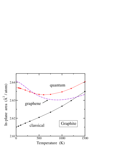
Figure 7: Temperature dependence of the in-plane area per atom, $A_{p}$, obtained from classical (circles) and PIMD (squares) simulations for $n=240$. Error bars are less than the symbol size. Solid lines are guides to the eye. A dashed line indicates the dependence of $A_{p}$ on $T$ for a graphene monolayer, as derived from PIMD simulations for the same system size.

In the graphene literature, it has been discussed with great detail the behavior of the in-plane area of the 2D material, which in the case of graphite corresponds to the area $L_{x}L_{y}$ on the $xy$ plane of the simulation box. Here we will consider the in-plane area per atom, $A_{p}=L_{x}L_{y}/n$. In Fig. 7 we show the temperature dependence of $A_{p}$ for unstressed graphite, as derived from classical MD (circles) and PIMD simulations (squares). At first sight one observes an important difference between the quantum and classical results. In the quantum data we find a decrease in $A_{p}$ for rising $T$ until a temperature of about 600 K, for which it reaches a minimum, and an increase in $A_{p}$ at higher $T$. In contrast, in the classical data we obtain a rise (roughly linear) of $A_{p}$ at low $T$, and an increase faster than linear at $T>500$ K. At $T=1500$ K the difference between classical and quantum data for $A_{p}$ is still much larger than the error bars of the simulation results (smaller than the symbol size in Fig. 7).

In the low-temperature limit ($T\to 0$), the in-plane area $A_{p}$ derived from PIMD simulations converges to 2.6371 Ų/atom, with a C–C bond length $d_{\rm C-C}=$ 1.4276 Å. For the classical minimum we find a value $A_{0}=2.6149$ Ų/atom, which corresponds to a C–C distance $d_{0}=1.4188$ Å. This gives for the quantum result a zero-point expansion in the area $A_{p}$ of 0.022 Ų/atom, i.e. a relative increase of about 1%, associated to the rise in C–C bond length. Looking at the C–C distance for the classical minimum, $d_{0}$, we observe that there is a slight in-plane lattice contraction with respect to the cases of a graphene monolayer ($d_{0}$ = 1.4199 Å) and bilayer ($d_{0}$ = 1.4193 Å), as a consequence of interlayer interactions.Herrero and Ramírez (2016, 2019) We note that, although in the classical model one has planar carbon sheets for $T\to 0$, in the quantum zero-temperature limit the layers are not exactly planar, since there is an atomic zero-point motion in the out-of-plane $z$-direction.Herrero and Ramírez (2016); Ramírez and Herrero (2017)

For comparison with the results for graphite, we also present in Fig. 7 the area $A_{p}$ obtained from PIMD simulations of monolayer graphene with the same size $n=240$ (dashed line). In this case, the shape of the temperature dependence is similar to that of graphite, with a decrease in $A_{p}$ at low $T$ and an increase at high $T$. For graphene, however, the decrease is larger and the minimum of $A_{p}$ occurs at a higher temperature. At low $T$, the area $A_{p}$ of graphite is reduced by $4\times 10^{-3}$ Ų/atom with respect to a graphene monolayer, as a consequence of layer interactions.

The fact that $dA_{p}/dT<0$ at low temperature, as obtained in the quantum simulations, is due to the out-of-plane motion of the carbon atoms, which dominates over the thermal expansion of the C–C bonds in the graphite layers. This effect is not captured by a classical model for the atomic motion, as happens in classical MD simulations, where the relative contributions of the different vibrational modes are not correctly represented at low temperatures. At high $T$, the bond expansion dominates over the contraction associated to motion in the $z$-direction, so that $dA_{p}/dT>0$ in both classical and quantum models.

VI Thermal expansion

At low $T$ our PIMD simulations give for graphite with AB stacking an interlayer spacing $c$ = 3.3510 Å. For the classical model at $T=0$ (minimum energy configuration with planar graphene sheets) we find $c_{0}$ = 3.3372 Å. Thus, we have a zero-point expansion $\Delta c=1.4\times 10^{-2}$ Å. At $T$ = 300 K, we have $c$ = 3.3688 Å from PIMD simulations, not far from a distance of 3.3538 Å obtained by Baskin and Meyer from x-ray diffraction measurements at room temperature ($T=297$ K).Baskin and Meyer (1955) At 300 K, the difference between quantum and classical results is around four times smaller than for the low-temperature limit.

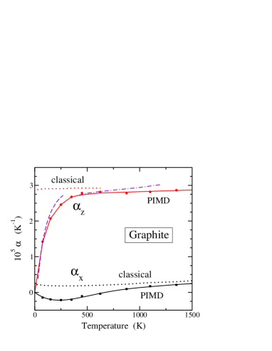
Figure 8: Linear thermal expansion coefficients of graphite vs temperature: $\alpha_{x}$ along the in-plane $x$-direction and $\alpha_{z}$ along the out-of-plane $z$-direction. Symbols represent data obtained from PIMD simulations for $n=960$ and solid lines are guides to the eye. Dotted lines indicate results derived from classical MD simulations. The dashed line represents data obtained for $\alpha_{z}$ by Bailey and YatesBailey and Yates (1970) from interferometric measurements at $T<300$ K. The dashed-dotted line is a fit to experimental data of $\alpha_{z}$ for $T>300$ K.Marsden et al. (2018)

From the mean interlayer spacing we consider the linear thermal expansion coefficient (TEC) $\alpha_{z}$, defined as

$$\alpha_{z}=\frac{1}{c}\left(\frac{\partial c}{\partial T}\right)_{\tau}\,.$$ (12)

This TEC for vanishing external stress has been commonly denoted as $\alpha_{c}$ in the literature, but we will call it here $\alpha_{z}$ for notation consistency. Data for $\alpha_{z}$ obtained from PIMD simulations of graphite are presented in Fig. 8 as solid circles. These data points were obtained from a numerical derivative of the mean layer spacing $c$ found in the simulations at several temperatures. One observes a fast rise of $\alpha_{z}$ in the low-temperature region up to around 200 K, and at higher $T$ this rise becomes much slower. At 300 K we find $\alpha_{z}=2.6\times 10^{-5}$ K^-1. For comparison, we also present in Fig. 8 results of classical MD simulations for $\alpha_{z}$ (dotted line). They converge at low $T$ to a value $\alpha_{z}=2.9\times 10^{-5}$ K^-1. Note the inconsistency of this classical result with the third law of Thermodynamics, which requires that TECs should vanish for $T\to 0$.Callen (1960); Ashcroft and Mermin (1976)

Experimental data for $\alpha_{z}$ of pyrolytic graphite at low $T$ were obtained by Bailey and YatesBailey and Yates (1970) from interferometric measurements (dashed line in Fig. 8). The dashed-dotted line indicates a fit to experimental data from several sources at $T>300$ K, presented by Marsden et al.Marsden et al. (2018) Both dashed and dashed-dotted lines derived from experimental data do not fit well one with the other close to room temperature, due to the dispersion of data in different source references. At $T>500$ K we observe that the TEC $\alpha_{z}$ obtained from our PIMD simulations rises slower than the line fitted to experimental data in Ref. Marsden et al., 2018.

In the $xy$ layer plane, we consider a linear TEC defined as

$$\alpha_{x}=\frac{1}{L_{x}}\left(\frac{\partial L_{x}}{\partial T}\right)_{\tau}\,.$$ (13)

In Fig. 8 (bottom) we display $\alpha_{x}$ obtained from PIMD simulations of graphite up to 1500 K (solid squares). The solid line represents a polynomial fit to the data points. At low temperature this TEC is negative and reaches a minimum at $T_{m}\approx 250$ K. For $T>T_{m}$, $\alpha_{x}$ increases for rising temperature and becomes positive at $T_{m}\approx 600$ K, which coincides with the temperature at which the in-plane area $A_{p}$ attains its minimum value, as shown in Fig. 7. For comparison, the dotted line in Fig. 8 (bottom) represents the results obtained for $\alpha_{x}$ from classical MD simulations. This classical $\alpha_{x}$ takes positive values in the whole temperature region considered here, and converges at low $T$ to a (nonphysical) value of $2.2\times 10^{-6}$ K^-1. The quantum data for $\alpha_{x}$ are below the classical ones, and for $T>1500$ K they are close one to the other.

Our results for $\alpha_{x}$ show a temperature dependence similar to those obtained earlier employing other theoretical techniques, in particular that found by Mounet and MarzariMounet and Marzari (2005) from a combination of DFT calculations with a QHA for the vibrational modes. These authors found for $\alpha_{x}$ a minimum of $-1.2\times 10^{-6}$ K^-1 for $T\approx 250$ K and a vanishing TEC for $T\approx 500$ K. Experimental results for the TEC $\alpha_{x}$ show a minimum at a temperature between 200 and 300 K, similarly to the data obtained from our quantum simulations.Kellett and Richards (1964); Morgan (1972); Marsden et al. (2018) Several experimental data sets display a minimum of about $-1.5\times 10^{-6}$ K^-1, which turns out to be somewhat less than our data presented in Fig. 8.

VII Linear elastic constants at finite temperatures

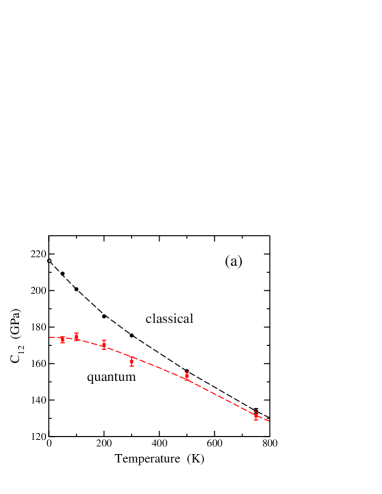
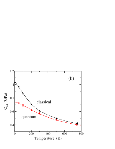
Figure 9: Temperature dependence of the elastic constants: (a) $C_{12}$ and (b) $C_{44}$, as derived from classical MD (circles) and PIMD (squares) simulations in the $NVT$ ensemble. Open circles in (a) and (b) represent the classical value at $T=0$, calculated from the phonon dispersion curves. Error bars, when not shown, are in the order of the symbol size. Lines are guides to the eye.

In this section we present and discuss nuclear quantum effects in the elastic stiffness constants of graphite. Such effects are present in general for the different elastic constants, mainly at low temperature, but they turn out to be especially large for $C_{12}$ and $C_{44}$. In Fig. 9(a) we present the temperature dependence of the elastic constant $C_{12}$, as derived from our classical (circles) and PIMD (squares) simulations. The classical finite-temperature results converge at low $T$ to the value obtained from the phonon dispersion, indicated by an open circle in Fig. 9(a). In the limit $T\to 0$, this elastic constant is found to decrease from the classical value of 216 GPa to 174 GPa due to zero-point motion. This represents a reduction of a 19% with respect to the classical result. At room temperature the quantum reduction amounts to a 7%.

In Fig. 9(b) we display the dependence of $C_{44}$ on temperature for both quantum (squares) and classical (circles) cases. The open circle at $T=0$ represents the value calculated from the phonon dispersion curves as explained in Sec. III ($C_{44}=1.03(2)$ GPa). The quantum results converge at low $T$ to $C_{44}=0.74$ GPa. This elastic constant is particularly interesting from the viewpoint of quantum effects. Given its small value in comparison to other stiffness constants of graphite, at low temperature the quantum correction with respect to the classical result is very large. In the limit $T\to 0$, it means a relative reduction of $C_{44}$ by a 28%.

Concerning nuclear quantum effects, something similar occurs for other elastic stiffness constants, as $C_{11}$ and $C_{33}$, for which results of classical and PIMD simulations are given in Table III at $T=$ 300 and 750 K, as well as for the low-$T$ limit. In all cases, the classical value at $T=0$ is calculated from the phonon dispersion bands and lattice strains, as explained in Sec. III. The low-temperature quantum values are obtained from an extrapolation of finite-temperature PIMD results. For $C_{11}$ and $C_{33}$, zero-point motion causes a decrease of 1.5% and 3.0% with respect to the classical value, respectively. We do not clearly observe any quantum effect in $C_{13}$. In fact, for this stiffness constant the results of PIMD and classical MD simulations coincide within error bars in the temperature region considered here.

It is worthwhile commenting on the relation between the temperature dependence of the linear elastic constants shown in Fig. 9 and the quantum delocalization of atomic nuclei. For $C_{12}$ and $C_{44}$, we find in the classical results a decrease as temperature is raised. This is related to classical thermal motion of the carbon atoms, which grows with temperature as indicated by the MSD shown in Fig. 1. In the results of our quantum PIMD simulations we observe an important decrease in the zero-temperature elastic constants, due to zero-point delocalization (finite MSD), with respect to the classical values, where the atomic MSD vanishes. As temperatures increases, the quantum and classical results converge one to the other, as happens for the MSD. Something similar can be said for the results of the bulk modulus presented below in Sec. VIII.

Table 4: Elastic stiffness constants, bulk modulus $B$, and Poisson’s ratio $\nu$ of graphite obtained from various experimental techniques by different authors at ambient conditions. Data for $C_{ij}$ and $B$ are given in GPa. The bulk modulus $B$ is obtained in each case from the elastic constants by using Eq. (16).

	BlaksleeBlakslee et al. (1970)	BosakBosak et al. (2007)	NicklowNicklow et al. (1972)
$C_{11}$	1060(20)	1109(16)	1440(200)
$C_{12}$	180(20)	139(36)	—
$C_{13}$	15(5)	0(3)	—
$C_{33}$	36.5(1)	38.7(7)	37.1(5)
$C_{44}$	0.27(9)	5.0(3)	4.6(2)
$B$	35.8(2)	36.4(11)	—
$\nu$	0.17	0.13	—

In Table IV we present values of the elastic stiffness constants derived from experimental data by several authors, from a combination of ultrasonic, sonic resonance, and static test methods,Blakslee et al. (1970) as well as inelastic x-ray scattering,Bosak et al. (2007) and inelastic neutron scattering along with a force model.Nicklow et al. (1972) There appears some dispersion in these results derived from experiments at ambient conditions, in particular for $C_{13}$ and $C_{44}$, as can be seen in our Table IV and in Refs. Blakslee et al., 1970; Bosak et al., 2007. For $C_{44}$ these values range from 5.0 GPa to less than 1 GPa. The low value $C_{44}=0.27(9)$ GPa obtained by Blakslee et al.Blakslee et al. (1970) may be due to the presence of dislocations in the studied material, as suggested by the authors. In a later paper, Seldin and NezbedaSeldin and Nezbeda (1970) found that this elastic constant rises when the graphite samples are irradiated with neutrons at several temperatures. These authors found that natural graphite crystals have after irradiation a shear modulus $C_{44}$ in the range 1.6–4.6 GPa. Experimental data for $C_{13}$ of graphite are scarce, and different techniques have yielded diverse outcomes. The results found by Bosak et al.Bosak et al. (2007) were compatible with a vanishing $C_{13}$ (within their error bar).

In Table V we give values of the elastic constants of graphite calculated by various research groups. Several calculations were carried out in the framework of DFT, with both local-density approximation (LDA) and generalized-gradient approximation (GGA).Boettger (1997); Hasegawa and Nishidate (2004); Mounet and Marzari (2005) Moreover, Jansen and FreemanJansen and Freeman (1987) employed the full-potential linearized augmented-plane wave (FLAPW) method, and Michel and Verberck obtained the elastic constants from the phonon spectrum calculated with an effective potential.Michel and Verberck (2008) In spite of the general reliability of these theoretical procedures, there are some discrepancies between the results of the different research groups. A common feature of the data derived from DFT calculations is that they yielded $C_{13}<0$, as shown in Table V. Although this is not forbidden for the stability of hexagonal crystals,Mouhat and Coudert (2014) we are not aware of any experimental work on graphite where $C_{13}$ was found to be negative. We also note the anomalous (very small) value obtained for $C_{33}$ in Ref. Hasegawa and Nishidate, 2004 from DFT-GGA calculations, which seems to be due to a largely underestimated interlayer interaction. Our main conclusion concerning the linear elastic constants of graphite is that the intrinsic difficulty of calculating the elastic constants of this largely anisotropic material, is still more complicated at temperatures lower than the Debye temperature of the material, where nuclear quantum effects are relevant.

Table 5: Elastic stiffness constants, bulk modulus, and Poisson’s ratio of graphite obtained from various calculations based on density-functional theory with LDA and GGA, as well as FLAPW and lattice dynamics (Latt. dyn.). Values indicated with an asterisk (^∗) correspond to $C_{11}+C_{12}$. Data for $C_{ij}$ and $B$ are given in GPa. The bulk modulus $B$ is obtained in each case from the elastic constants by means of Eq. (16).

	LDABoettger (1997)	FLAPWJansen and Freeman (1987)	LDA, GGAHasegawa and Nishidate (2004)	LDA, GGAMounet and Marzari (2005)	Latt. dyn.Michel and Verberck (2008)
$C_{11}$	1279.6∗	1430∗	—	1118, 1079	1211.3
$C_{12}$	—	—	—	235, 217	275.5
$C_{13}$	–0.5	–12	—	–2.8, –0.5	0.59
$C_{33}$	40.8	56	30.4, 0.8	29.5, 42.2	36.79
$C_{44}$	—	—	—	4.5, 3.9	4.18
$B$	38.3	50.2	—	28.0, 39.6	35.1
$\nu$	—	—	—	0.210, 0.201	0.227

From the elastic stiffness constants one can obtain the Poisson’s ratio $\nu$, which is a measure of the relation between the transverse and longitudinal strains under an applied stress. For graphite one has $\nu=C_{12}/C_{11}$. In Table III we give the Poisson’s ratio calculated from the elastic constants yielded by our classical and quantum simulations. In our results, $\nu$ is found to decrease as temperature is raised. In the low-temperature limit, nuclear quantum motion causes a reduction of $\nu$ from 0.215 to 0.175, i.e., it decreases by a 19%. At $T$ = 300 K the classical and quantum values are 0.181 and 0.169, respectively, with a decrease of a 7% due to quantum motion. At 750 K this decrease is small, about 1%.

In Table IV we give values of the Poisson’s ratio obtained from the elastic constants found in experimental works.Blakslee et al. (1970); Bosak et al. (2007) The value derived from the work of Blakslee et al.Blakslee et al. (1970) is close to our quantum result at $T=300$ K, and that from the paper by Bosak et al.Bosak et al. (2007) is somewhat lower. Data derived from theoretical methods given in Table V are close to our classical value at $T=0$, $\nu=0.215$. A larger collection of data for the Poisson’s ratio of graphite derived from theoretical methods is given in Ref. Politano and Chiarello, 2015. The data reported in the literature display a large dispersion, most of them lying in the region from 0.12 to 0.3. We note that the Poisson’s ratio usually considered for graphite is an in-plane variable, i.e., it refers to $x$ and $y$ directions. One can equally define an out-of-plane ratio $\nu_{xz}$, referring to $x$ and $z$ directions. In this case, $\nu_{xz}=C_{13}/C_{11}$, and we find from our PIMD simulations at 300 K: $\nu_{xz}=3.5\times 10^{-3}$.

VIII Bulk modulus

We present here results for the isothermal bulk modulus, $B=-V(\partial P/\partial V)_{T}$ , derived from our classical MD and quantum PIMD simulations. To check the overall consistency of our procedures, we obtain $B$ in three different ways: (1) calculating ${\partial P}/{\partial V}$ from a numerical differentiation for positive and negative hydrostatic pressures $P$ close to $P=0$, (2) from the volume fluctuations along $NPT$ simulation runs at temperature $T$, and (3) from the elastic constants obtained from the simulations.

In the isothermal-isobaric ensemble (our second method), the bulk modulus can be directly calculated from the mean-square fluctuations of the volume, $\sigma_{V}^{2}$, using the formulaLandau and Lifshitz (1980); Herrero (2008)

$$B=\frac{k_{B}TV}{\sigma_{V}^{2}}\;,$$ (14)

$k_{B}$ being Boltzmann’s constant. This expression has been employed earlier to obtain the bulk modulus of various kinds of solids from path-integral simulations.Herrero and Ramírez (2000); Herrero (2008)

The bulk modulus of graphite can be also calculated from the elastic constants of the material (our third procedure). For a hydrostatic pressure $P$, we have $\tau_{xx}=\tau_{yy}=\tau_{zz}=-P$, so that

$$\frac{\Delta V}{V}=e_{xx}+e_{yy}+e_{zz}=-(2S_{11}+2S_{12}+4S_{13}+S_{33})P\;,$$ (15)

and using the relations between stiffness and compliance constants,Marsden et al. (2018); Rabiei et al. (2020) we find

$$B=-V\frac{\partial P}{\partial V}=\frac{(C_{11}+C_{12})\,C_{33}-2C_{13}^{2}}{C_{11}+C_{12}+2C_{33}-4C_{13}}\;,$$ (16)

as in Refs. Jansen and Freeman, 1987; Boettger, 1997.

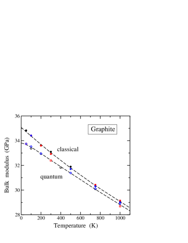
Figure 10: Temperature dependence of the bulk modulus of graphite, obtained from PIMD (open symbols) and classical MD simulations (solid symbols). The data shown in both cases were obtained by following three different procedures: (1) numerical derivative $dP/dV$ from various hydrostatic pressures $P$ (squares), (2) fluctuation formula in Eq. (14) (circles), and (3) from the elastic constants using Eq. (16) (diamonds). Error bars are on the order of the symbol size. Dashed lines are guides to the eye.

The temperature dependence of the bulk modulus $B$ of graphite derived from our simulations is shown in Fig. 10. Solid and open symbols represent results of classical and quantum simulations, respectively. In each case, symbols represent data obtained from (1) numerical derivative $dP/dV$ (squares), (2) fluctuation formula (circles), and (3) elastic constants (diamonds). The values obtained for the bulk modulus from the three methods agree well in the whole temperature range considered here, for both quantum and classical data. In the limit $T\to 0$, we find $B$ = 35.1 and 33.8 GPa for the classical and quantum models, respectively. This means a reduction of the bulk modulus by a 4% due to zero-point motion of the C atoms.

In Table III we give values of the bulk modulus $B$ of graphite calculated using Eq. (16) from the stiffness constants derived from our classical and quantum simulations at $T$ = 300 and 750 K, as well as for the zero-temperature limit. Values of $B$ obtained from the elastic constants yielded by experimental and theoretical methods are given in Tables IV and V, respectively. From an analysis of the equation of state of graphite at room temperature, Hanfland et al.Hanfland et al. (1989) found at ambient pressure $B$ = 33.8(30) GPa, a little higher than our quantum result at 300 K ($B$ = 32.3 GPa). Zhao and SpainZhao and Spain (1989) obtained a somewhat larger value, $B$ = 35.8(16), from x-ray diffraction experiments. Tohei et al.Tohei et al. (2006) found $B$ = 28.7 GPa at 300 K from LDA-DFT calculations combined with a QHA for the lattice modes.

One can also define an “isotropic bulk modulus” $B_{\rm iso}$ for isotropic changes of the volume,Jansen and Freeman (1987) which means $e_{xx}=e_{yy}=e_{zz}=e$ and $\Delta V/V=3e$. One thus has a hydrostatic pressure

$$P=-\frac{1}{3}(\tau_{xx}+\tau_{yy}+\tau_{zz})\;,$$ (17)

which gives

$$B_{\rm iso}=-V\frac{\partial P}{\partial V}=\frac{1}{9}\,\left(2C_{11}+2C_{12}+4C_{13}+C_{33}\right)\;.$$ (18)

For the classical limit at $T=0$ we have $B_{\rm iso}$ = 276.6 GPa, and from our PIMD simulations we find for $T\to 0$: $B_{\rm iso}$ = 263.5 GPa. At $T$ = 300 K, the classical and quantum simulations yield 259.6 and 254.6 GPa, respectively.

IX Summary

PIMD simulations allow us to quantify nuclear quantum effects in structural and elastic properties in condensed matter. For graphite, in particular, we have seen that such quantum effects are appreciable for $T$ in the order of 500 K, and even higher for some variables. At low temperature, the quantum zero-point expansion of the graphite volume is nonnegligible, and amounts to 1.3% of the classical value. In spite of the large anisotropy of graphite, we have found that the expansion due to zero-point motion is nearly isotropic, i.e., the relative increases in in-plane and out-of-plane directions are approximately the same.

The thermal contraction of the in-plane area ($\alpha_{x}<0$) observed in x-ray diffraction experiments at low temperature is reproduced by our quantum simulations, contrary to classical MD, where a positive in-plane thermal expansion is found in the whole temperature range studied here. Given that a negative $\alpha_{x}$ in layered materials is caused by out-of-plane atomic motion, the in-plane contraction of graphite is essentially due to quantum motion of the C atoms in the $z$-direction. Also, the characteristic trend of $\alpha_{x}$ (negative at low $T$ and positive at high $T$) is a clear signature of anharmonicity in the vibrational modes, indicating a coupling between in-plane and out-of-plane modes.

Quantization of lattice vibrations gives rise to changes in the elastic properties of graphite with respect to a classical model. At low temperature, the most significant relative changes in the elastic stiffness constants correspond to $C_{12}$ and $C_{44}$, where quantum corrections cause a reduction of 19% and 28%, respectively. The bulk modulus and Poisson’s ratio decrease by a 4% and 19% at low $T$ because of zero-point motion of the carbon atoms. In general, our results indicate that graphite is “softer” than predicted by classical simulations.

In connection with $C_{13}$, it is still open the question why several ab-initio calculations have yielded negative values, which has not been observed in experimental studies. We found here positive values for this elastic constant, but we did not observe any quantum effect on it. All this could be due to a lack of precision in the description of interlayer van-der-Waals-like interactions.

We finally note the consistency of the simulation results with the third law of thermodynamics. This means, in particular, that for $T\to 0$, thermal expansion coefficients should vanish. Moreover, the temperature derivatives of the elastic stiffness constants and bulk modulus should also vanish.