Aerial Base Station Placement Leveraging Radio Tomographic Maps

Abstract

Mobile base stations on board unmanned aerial vehicles (UAVs) promise to deliver connectivity to those areas where the terrestrial infrastructure is overloaded, damaged, or absent. A fundamental problem in this context involves determining a minimal set of locations in 3D space where such aerial base stations (ABSs) must be deployed to provide coverage to a set of users. While nearly all existing approaches rely on average characterizations of the propagation medium, this work develops a scheme where the actual channel information is exploited by means of a radio tomographic map. A convex optimization approach is presented to minimize the number of required ABSs while ensuring that the UAVs do not enter no-fly regions. A simulation study reveals that the proposed algorithm markedly outperforms its competitors.

1 Introduction

The rapid evolution of the technology of unmanned aerial vehicles (UAVs) has spurred extensive research to complement terrestrial communication infrastructure with base stations mounted on board UAVs [1]. The main use case of such aerial base stations (ABSs) is to provide connectivity in areas where it is insufficient or not available, e.g. because they are remote or because of a natural disaster. The research question that arises is at which locations one or multiple ABSs need to be deployed to provide coverage to the ground terminals (GTs).

This question has been extensively investigated for a single ABS; see e.g. [2, 3, 4, 5]. Other schemes have been proposed to set the 2D position of multiple ABSs in a horizontal plane of a given height; see e.g. [6]. In contrast, the focus here is on algorithms capable of determining the 3D position of the ABSs. Existing works in this context are classified next according to how they account for the propagation channel between the ABSs and the GTs. First, some schemes [7] do not model or learn the channel and, therefore, the suitability of a location cannot be determined before an ABS visits it, which drastically increases the time to find a suitable placement. Besides approaches that assume free-space propagation [8], a large number of works rely on the empirical model from [9]; see e.g. [10, 11, 12, 13, 14].The main limitation is that such models provide shadowing values in average scenarios, e.g. in a generic urban environment, but are likely to yield highly suboptimal placements in a specific environment. This limitation is addressed in [15, 16] by using 3D models of the deployment scenario. Unfortunately, 3D models are seldom available and, even when they are, their resolution is insufficient for reasonably predicting the channel in conventional bands or, for example, when a GT is inside a building.

In contrast, the present paper proposes a scheme where the air-to-ground channel of the specific deployment scenario is learned by relying on the notion of radio tomography [17, 18]. A radio map that provides the attenuation between arbitrary points of space is constructed based on measurements collected by the GTs and ABSs. To accommodate the special requirements of air-to-ground radio maps, the conventional approach to radio tomography, which has a cubic complexity in the size of the grid, is here replaced with a linear complexity algorithm. Using this radio map, a placement algorithm is proposed to minimize the number of ABSs required to guarantee a minimum rate for all GTs. Unlike most competing algorithms, it is based on a convex program, it can accommodate no-fly zones, and has low computational complexity. The third contribution is an open source simulator that allows testing and developing algorithms for ABS placement; see Fig. 1.

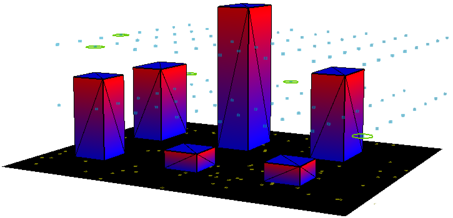
Fig. 1: Example of ABS placement in an urban environment with the developed simulator. GTs are represented by markers on the ground, grid points by blue dots, and ABS positions by green circles.

Paper structure. Sec. 2 and formulates the problem. The construction and evaluation of radio maps is described in Sec. 3. An algorithm for ABS placement using radio maps is then proposed in Sec. 4. Performance evaluation is carried out in Sec. 5 by means of the developed simulator. Finally, Secs. 6 and 7 respectively discuss the related work and present the main conclusions. The supplementary material contains an algorithm for approximating tomographic integrals and the derivation of the placement algorithm.

Notation. $\mathbb{R}_{+}$ is set of non-negative real numbers. Boldface uppercase (lowercase) letters denote matrices (column vectors). $a[i]$ represents the $i$-th entry of vector $\bm{a}$. Notation $\bm{0}$ (respectively $\bm{1}$) refers to the matrix of the appropriate dimensions with all zeros (ones). $\|\bm{A}\|_{{\color[rgb]{0,0,0}\text{F}}}$ denotes Frobenius norm of matrix $\bm{A}$, whereas $\|\bm{a}\|_{p}$ denotes the $\ell_{p}$-norm of vector $\bm{a}$. With no subscript, $\|\bm{a}\|$ stands for the $\ell_{2}$-norm. Inequalities between vectors or matrices must be understood entrywise.

2 Model and Problem Formulation

Consider ${{\color[rgb]{0,0,0}M}}$ users or ground terminals (GTs) located at positions $\{{{\color[rgb]{0,0,0}\bm{x}}}^{\text{GT}}_{1},\ldots,{{\color[rgb]{0,0,0}\bm{x}}}^{\text{GT}}_{{\color[rgb]{0,0,0}M}}\}\subset{{\color[rgb]{0,0,0}\mathcal{X}}}\subset\mathbb{R}^{3}$, where region ${{\color[rgb]{0,0,0}\mathcal{X}}}$ will typically include points on the ground and inside buildings. To provide connectivity to the GTs, ${{\color[rgb]{0,0,0}N}}$ ABSs are deployed at positions $\{{{\color[rgb]{0,0,0}\bm{x}}}^{\text{ABS}}_{1},\ldots,{{\color[rgb]{0,0,0}\bm{x}}}^{\text{ABS}}_{{\color[rgb]{0,0,0}N}}\}\subset{{\color[rgb]{0,0,0}\mathcal{F}}}\subset\mathbb{R}^{3}$, where ${{\color[rgb]{0,0,0}\mathcal{F}}}$ comprises all locations where a UAV is allowed to fly. This excludes no-fly zones, airspace occupied by buildings, and altitudes out of legal limits. To simplify the exposition, the focus will be on the downlink and it will be assumed that the channel is not frequency dispersive. The rate of the communication link between the ${{\color[rgb]{0,0,0}m}}$-th GT and an ABS at position ${{\color[rgb]{0,0,0}\bm{x}}}^{\text{ABS}}\in{{\color[rgb]{0,0,0}\mathcal{X}}}$ is determined by the channel gain and noise power. The former is given by

$${\color[rgb]{0,0,0}\gamma}_{{\color[rgb]{0,0,0}m}}({{\color[rgb]{0,0,0}\bm{x}}}^{\text{ABS}})=20\log_{10}\left(\frac{{\color[rgb]{0,0,0}\lambda}}{4\pi\|{{\color[rgb]{0,0,0}\bm{x}}}^{\text{GT}}_{{\color[rgb]{0,0,0}m}}-{{\color[rgb]{0,0,0}\bm{x}}}^{\text{ABS}}\|}\right)-{\color[rgb]{0,0,0}\xi}({{\color[rgb]{0,0,0}\bm{x}}}^{\text{GT}}_{{\color[rgb]{0,0,0}m}},{{\color[rgb]{0,0,0}\bm{x}}}^{\text{ABS}}),$$ (1)

where ${\color[rgb]{0,0,0}\lambda}$ is the wavelength associated with the carrier frequency of the transmission and function ${\color[rgb]{0,0,0}\xi}$ denotes shadowing. Small-scale fading is ignored for simplicity, but the ensuing formulation can be adapted to accommodate the associated uncertainty. The capacity is

$${\color[rgb]{0,0,0}C}_{{\color[rgb]{0,0,0}m}}({{\color[rgb]{0,0,0}\bm{x}}}^{\text{ABS}})={\color[rgb]{0,0,0}W}\log_{2}\left(1+{{\color[rgb]{0,0,0}P_{\text{TX}}}10^{{\color[rgb]{0,0,0}\gamma}_{{\color[rgb]{0,0,0}m}}({{\color[rgb]{0,0,0}\bm{x}}}^{\text{ABS}})/10}}/{{\color[rgb]{0,0,0}\sigma^{2}}}\right),$$ (2)

where ${\color[rgb]{0,0,0}W}$ denotes bandwidth, ${\color[rgb]{0,0,0}P_{\text{TX}}}$ the transmit power, and ${\color[rgb]{0,0,0}\sigma^{2}}$ the noise power. Since the ${{\color[rgb]{0,0,0}m}}$-th GT may connect to one or multiple ABSs, it may receive a rate up to $\sum_{{\color[rgb]{0,0,0}n}}{\color[rgb]{0,0,0}C}_{{\color[rgb]{0,0,0}m}}({{\color[rgb]{0,0,0}\bm{x}}}^{\text{ABS}}_{{\color[rgb]{0,0,0}n}})$. As usual in the literature, it is assumed that the backhaul connection of the ABSs has sufficiently high capacity, yet the proposed scheme can be generalized to accommodate backhaul constraints.

The problem is to find a minimal set of ABS locations that guarantees a minimum rate for every user. This criterion arises naturally in some of the main use cases of UAV-assisted networks such as emergency response or disaster management. Formally, the problem can be stated as follows:

$$\mathop{\text{minimize}}_{{{\color[rgb]{0,0,0}N}},\{{{\color[rgb]{0,0,0}\bm{x}}}^{\text{ABS}}_{{\color[rgb]{0,0,0}n}}\}_{{{\color[rgb]{0,0,0}n}}=1}^{{\color[rgb]{0,0,0}N}}}~{} {{\color[rgb]{0,0,0}N}}$$ (3a)

$$\mathop{\text{s.t.}}~{} \textstyle\sum_{{\color[rgb]{0,0,0}n}}{\color[rgb]{0,0,0}C}_{{\color[rgb]{0,0,0}m}}({{\color[rgb]{0,0,0}\bm{x}}}^{\text{ABS}}_{{\color[rgb]{0,0,0}n}})\geq{\color[rgb]{0,0,0}{\color[rgb]{0,0,0}r}}_{\text{min}},~{}{{\color[rgb]{0,0,0}m}}=1,\ldots,{{\color[rgb]{0,0,0}M}},$$ (3b)

$${{\color[rgb]{0,0,0}\bm{x}}}^{\text{ABS}}_{{\color[rgb]{0,0,0}n}}\in{{\color[rgb]{0,0,0}\mathcal{F}}},~{}~{}{{\color[rgb]{0,0,0}n}}=1,\ldots,{{\color[rgb]{0,0,0}N}}.$$ (3c)

To simplify notation, the same rate ${\color[rgb]{0,0,0}{\color[rgb]{0,0,0}r}}_{\text{min}}$ is assumed across GTs, but different rates can be set up to straightforward modifications.

3 Tomographic Radio Maps

The first difficulty when solving (3) is that the function ${\color[rgb]{0,0,0}C}_{{\color[rgb]{0,0,0}m}}({{\color[rgb]{0,0,0}\bm{x}}}^{\text{ABS}})$ is unknown since the shadowing term ${\color[rgb]{0,0,0}\xi}({{\color[rgb]{0,0,0}\bm{x}}}^{\text{GT}}_{{\color[rgb]{0,0,0}m}},{{\color[rgb]{0,0,0}\bm{x}}}^{\text{ABS}})$ in (1) is unknown. The approach proposed here is to rely on a radio map that provides ${\color[rgb]{0,0,0}\xi}({{\color[rgb]{0,0,0}\bm{x}}}^{\text{GT}},{{\color[rgb]{0,0,0}\bm{x}}}^{\text{ABS}})$ for all ${{\color[rgb]{0,0,0}\bm{x}}}^{\text{GT}}$ and ${{\color[rgb]{0,0,0}\bm{x}}}^{\text{ABS}}$. Such a map can be constructed by means of the so-called tomographic (or NeSh) model [17], as considered in the literature of channel-gain cartography; see [19] and references therein. However, the existing works in this context focus on ground-to-ground channels. Constructing radio maps of air-to-ground channels involves special challenges that render existing approaches unsuitable, as discussed later.

The radio tomographic model [17] prescribes that

$${\color[rgb]{0,0,0}\xi}({{\color[rgb]{0,0,0}\bm{{{\color[rgb]{0,0,0}x}}}}}_{1},{{\color[rgb]{0,0,0}\bm{{{\color[rgb]{0,0,0}x}}}}}_{2})=\frac{1}{\|{{\color[rgb]{0,0,0}\bm{{{\color[rgb]{0,0,0}x}}}}}_{1}-{{\color[rgb]{0,0,0}\bm{{{\color[rgb]{0,0,0}x}}}}}_{2}\|_{2}^{1/2}}\int_{{{\color[rgb]{0,0,0}\bm{{{\color[rgb]{0,0,0}x}}}}}_{1}}^{{{\color[rgb]{0,0,0}\bm{{{\color[rgb]{0,0,0}x}}}}}_{2}}{\color[rgb]{0,0,0}l}({{\color[rgb]{0,0,0}\bm{{{\color[rgb]{0,0,0}x}}}}})d{{\color[rgb]{0,0,0}\bm{{{\color[rgb]{0,0,0}x}}}}},$$ (4)

where the function ${\color[rgb]{0,0,0}l}$ inside the line integral is termed spatial loss field (SLF) and quantifies the local attenuation (absorption) that a signal suffers at each position. The SLF can be estimated in a first stage before solving (3) by collecting measurements of the form $({{\color[rgb]{0,0,0}\bm{x}}}^{\text{ABS}},{{\color[rgb]{0,0,0}\bm{x}}}^{\text{GT}},{\color[rgb]{0,0,0}\gamma}_{{\color[rgb]{0,0,0}m}}({{\color[rgb]{0,0,0}\bm{x}}}^{\text{ABS}}))$ and applying standard estimation techniques; see e.g. [20, 21, 19].

In practice, to estimate ${\color[rgb]{0,0,0}l}$ and evaluate (4), function ${\color[rgb]{0,0,0}l}$ needs to be discretized by storing its values ${\color[rgb]{0,0,0}l}({{\color[rgb]{0,0,0}\bm{x}}}^{{\color[rgb]{0,0,0}\bar{\mathcal{X}}}}_{1}),\ldots,{\color[rgb]{0,0,0}l}({{\color[rgb]{0,0,0}\bm{x}}}^{{\color[rgb]{0,0,0}\bar{\mathcal{X}}}}_{{\color[rgb]{0,0,0}Q}})$ on a 3D regular grid of ${{\color[rgb]{0,0,0}Q}}$ points ${{\color[rgb]{0,0,0}\bar{\mathcal{X}}}}:=\{{{\color[rgb]{0,0,0}\bm{x}}}^{{\color[rgb]{0,0,0}\bar{\mathcal{X}}}}_{1},\ldots,{{\color[rgb]{0,0,0}\bm{x}}}^{{\color[rgb]{0,0,0}\bar{\mathcal{X}}}}_{{\color[rgb]{0,0,0}Q}}\}$. The conventional approach approximates (4) as a weighted sum [22] of the values ${\color[rgb]{0,0,0}l}({{\color[rgb]{0,0,0}\bm{x}}}^{{\color[rgb]{0,0,0}\bar{\mathcal{X}}}}_{{\color[rgb]{0,0,0}q}})$ for which the centroid ${{\color[rgb]{0,0,0}\bm{x}}}^{{\color[rgb]{0,0,0}\bar{\mathcal{X}}}}_{{\color[rgb]{0,0,0}q}}$ lies inside an ellipsoid with foci at ${{\color[rgb]{0,0,0}\bm{{{\color[rgb]{0,0,0}x}}}}}_{1}$ and ${{\color[rgb]{0,0,0}\bm{{{\color[rgb]{0,0,0}x}}}}}_{2}$; see the ellipses in Fig. 2 for a depiction in 2D. Unfortunately, it can be easily seen from Fig. 2 that the resulting approximation of ${\color[rgb]{0,0,0}\xi}({{\color[rgb]{0,0,0}\bm{{{\color[rgb]{0,0,0}x}}}}}_{1},{{\color[rgb]{0,0,0}\bm{{{\color[rgb]{0,0,0}x}}}}}_{2})$ is a discontinuous function of ${{\color[rgb]{0,0,0}\bm{{{\color[rgb]{0,0,0}x}}}}}_{1}$ and ${{\color[rgb]{0,0,0}\bm{{{\color[rgb]{0,0,0}x}}}}}_{2}$. It may even be 0 even when ${\color[rgb]{0,0,0}l}({{\color[rgb]{0,0,0}\bm{x}}}^{{\color[rgb]{0,0,0}\bar{\mathcal{X}}}}_{{\color[rgb]{0,0,0}q}})\neq 0~{}\forall{{\color[rgb]{0,0,0}q}}$. To minimize these effects, the grid point spacing needs to be small relative to the length of the minor axis, which is commonly set in the order of the wavelength. Thus, for standard centimetric wavelengths and regions ${{\color[rgb]{0,0,0}\mathcal{X}}}$ with sides in the order of km and height in the order of 100 m, ${{\color[rgb]{0,0,0}Q}}$ must be in the order of $10^{14}$, which is prohibitively high. Finally, the complexity of such an approximation is $\mathcal{O}({{\color[rgb]{0,0,0}{{\color[rgb]{0,0,0}Q}}}}_{0}^{3})$ for a ${{\color[rgb]{0,0,0}{{\color[rgb]{0,0,0}Q}}}}_{0}\times{{\color[rgb]{0,0,0}{{\color[rgb]{0,0,0}Q}}}}_{0}\times{{\color[rgb]{0,0,0}{{\color[rgb]{0,0,0}Q}}}}_{0}$ grid.

To remedy these issues, this paper advocates approximating the integral in (4) as a line integral of a piecewise constant approximation of ${\color[rgb]{0,0,0}l}$, as already hinted in [21] for tomographic imaging. This involves obtaining the intersections between the the voxel boundaries and the line segment that connects the transmitter to the receiver locations; see the colored segment in Fig. 2. A possible implementation along the lines of [23, Sec. I-B-1] is presented in the supplementary material, but others are possible. The resulting approximation is continuous, can be used with large grid point spacing, and can be computed with complexity only $\mathcal{O}({{\color[rgb]{0,0,0}{{\color[rgb]{0,0,0}Q}}}}_{0})$ for a ${{\color[rgb]{0,0,0}{{\color[rgb]{0,0,0}Q}}}}_{0}\times{{\color[rgb]{0,0,0}{{\color[rgb]{0,0,0}Q}}}}_{0}\times{{\color[rgb]{0,0,0}{{\color[rgb]{0,0,0}Q}}}}_{0}$ grid.

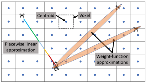
Fig. 2: 2D illustration of the conventional weight-function approximation of the tomographic integral (4) (orange ellipses) and the approximation adopted here (colored line segment). Observe that the upper ellipse contains no centroid and, therefore, the approximation will yield zero attenuation regardless of the values of the SLF.

4 Placement with Min-rate Guarantees

The approach in Sec. 3 makes it possible to find the shadowing between any two points and, therefore, the channel gain and capacity; cf. (1) and (2). The constraint in (3b) can thus be evaluated. Yet, solving (3) is challenging: even if ${{\color[rgb]{0,0,0}N}}$ were known and one just needed to find feasible $\{{{\color[rgb]{0,0,0}\bm{x}}}^{\text{ABS}}_{{\color[rgb]{0,0,0}n}}\}_{{{\color[rgb]{0,0,0}n}}=1}^{{\color[rgb]{0,0,0}N}}$, the problem would still be non-convex due to the constraints. To bypass this difficulty, the proposed approach involves discretizing the flight region ${{\color[rgb]{0,0,0}\mathcal{F}}}$ into a flight grid ${{\color[rgb]{0,0,0}\bar{\mathcal{F}}}}:=\{{{\color[rgb]{0,0,0}\bm{x}}}^{{\color[rgb]{0,0,0}\bar{\mathcal{F}}}}_{1},\ldots,{{\color[rgb]{0,0,0}\bm{x}}}^{{\color[rgb]{0,0,0}\bar{\mathcal{F}}}}_{{\color[rgb]{0,0,0}G}}\}\subset{{\color[rgb]{0,0,0}\mathcal{F}}}\subset\mathbb{R}^{3}$; see Fig. 1.

Since ${{\color[rgb]{0,0,0}\bar{\mathcal{F}}}}$ contains only points where an ABS can be placed, solving (3) amounts to finding the smallest subset of ${{\color[rgb]{0,0,0}N}}$ points of ${{\color[rgb]{0,0,0}\bar{\mathcal{F}}}}$ that satisfies (3b). To see this, replace ${{\color[rgb]{0,0,0}\bm{x}}}^{\text{ABS}}_{{\color[rgb]{0,0,0}n}}\in{{\color[rgb]{0,0,0}\mathcal{F}}}$ in (3c) with ${{\color[rgb]{0,0,0}\bm{x}}}^{\text{ABS}}_{{\color[rgb]{0,0,0}n}}\in{{\color[rgb]{0,0,0}\bar{\mathcal{F}}}}$ and let ${\color[rgb]{0,0,0}\alpha}_{{\color[rgb]{0,0,0}g}}$ be 1 if there is an ABE at ${{\color[rgb]{0,0,0}\bm{x}}}^{{\color[rgb]{0,0,0}\bar{\mathcal{F}}}}_{{\color[rgb]{0,0,0}g}}$ and 0 otherwise. The summation in (3b) can then be expressed as $\sum_{{\color[rgb]{0,0,0}g}}{\color[rgb]{0,0,0}\alpha}_{{\color[rgb]{0,0,0}g}}{\color[rgb]{0,0,0}C}_{{\color[rgb]{0,0,0}m}}({{\color[rgb]{0,0,0}\bm{x}}}^{{\color[rgb]{0,0,0}\bar{\mathcal{F}}}}_{{\color[rgb]{0,0,0}g}})$. Since the number of ABSs can be written as $\sum_{{\color[rgb]{0,0,0}g}}{\color[rgb]{0,0,0}\alpha}_{{\color[rgb]{0,0,0}g}}$, the discretized version of (3) becomes

$$\mathop{\text{minimize}}_{{\color[rgb]{0,0,0}\bm{\alpha}}\in\{0,1\}^{{{\color[rgb]{0,0,0}G}}}}\quad \textstyle\sum_{{{\color[rgb]{0,0,0}g}}}{\color[rgb]{0,0,0}\alpha}_{{\color[rgb]{0,0,0}g}}$$ (5a)

$$\mathop{\text{s.t.}}\quad \textstyle\sum_{{{\color[rgb]{0,0,0}g}}}{\color[rgb]{0,0,0}\alpha}_{{\color[rgb]{0,0,0}g}}{\color[rgb]{0,0,0}\bm{{\color[rgb]{0,0,0}c}}}_{{\color[rgb]{0,0,0}g}}\geq{\color[rgb]{0,0,0}{\color[rgb]{0,0,0}r}}_{\text{min}}\bm{1},$$ (5b)

where ${\color[rgb]{0,0,0}\bm{{\color[rgb]{0,0,0}c}}}_{{\color[rgb]{0,0,0}g}}:=[{\color[rgb]{0,0,0}C}_{1}({{\color[rgb]{0,0,0}\bm{x}}}^{{\color[rgb]{0,0,0}\bar{\mathcal{F}}}}_{{\color[rgb]{0,0,0}g}}),\ldots,{\color[rgb]{0,0,0}C}_{{\color[rgb]{0,0,0}M}}({{\color[rgb]{0,0,0}\bm{x}}}^{{\color[rgb]{0,0,0}\bar{\mathcal{F}}}}_{{\color[rgb]{0,0,0}g}})]^{\top}$. Problem (5) is of a combinatorial nature and can be solved for small ${{\color[rgb]{0,0,0}G}}$ by exhaustive search. However, the complexity of such a task is exponential and, therefore, it is preferable to adopt an approximation that can be efficiently computed. One possibility is to relax the constraint ${\color[rgb]{0,0,0}\bm{\alpha}}\in\{0,1\}^{{{\color[rgb]{0,0,0}G}}}$ as well as the objective and apply an interior-point solver. This approach is described in the supplementary material but not pursued here due to the well-known poor scalability of this kind of methods with the number of variables and constraints [24]. Indeed, in this application, ${{\color[rgb]{0,0,0}G}}$ can be in the order of millions, which would render the cubic complexity of interior-point methods prohibitive. Instead, this section presents a solver based on the alternating-direction method of multipliers (ADMM) [25] whose complexity is linear in ${{\color[rgb]{0,0,0}G}}$.

Suppose that there exists no grid point such that ${\color[rgb]{0,0,0}\bm{{\color[rgb]{0,0,0}c}}}_{{\color[rgb]{0,0,0}g}}=\bm{0}$. Otherwise, ${{\color[rgb]{0,0,0}\bm{x}}}^{{\color[rgb]{0,0,0}\bar{\mathcal{F}}}}_{{\color[rgb]{0,0,0}g}}$ can be disregarded without further implications. By applying the change of variables ${\color[rgb]{0,0,0}\alpha}_{{\color[rgb]{0,0,0}g}}{\color[rgb]{0,0,0}\bm{{\color[rgb]{0,0,0}c}}}_{{\color[rgb]{0,0,0}g}}\rightarrow{\color[rgb]{0,0,0}\bm{{\color[rgb]{0,0,0}r}}}_{{\color[rgb]{0,0,0}g}}$, it is clear that Problem (5) can be equivalently written as

$$\mathop{\text{minimize}}_{{\color[rgb]{0,0,0}\bm{R}}\in\mathbb{R}^{{{\color[rgb]{0,0,0}M}}\times{{\color[rgb]{0,0,0}G}}}}\quad \textstyle\sum_{{{\color[rgb]{0,0,0}g}}=1}^{{{\color[rgb]{0,0,0}G}}}\mathbb{I}[{\color[rgb]{0,0,0}\bm{{\color[rgb]{0,0,0}r}}}_{{\color[rgb]{0,0,0}g}}\neq\bm{0}]$$ (6a)

$$\mathop{\text{s.t.}}\quad \textstyle\sum_{{{\color[rgb]{0,0,0}g}}=1}^{{{\color[rgb]{0,0,0}G}}}{\color[rgb]{0,0,0}\bm{{\color[rgb]{0,0,0}r}}}_{{\color[rgb]{0,0,0}g}}\geq{\color[rgb]{0,0,0}{\color[rgb]{0,0,0}r}}_{\text{min}}\bm{1}$$ (6b)

$${\color[rgb]{0,0,0}\bm{{\color[rgb]{0,0,0}r}}}_{{\color[rgb]{0,0,0}g}}\in\{\bm{0},{\color[rgb]{0,0,0}\bm{{\color[rgb]{0,0,0}c}}}_{{\color[rgb]{0,0,0}g}}\},~{}{{\color[rgb]{0,0,0}g}}=1,\ldots,{{\color[rgb]{0,0,0}G}},$$ (6c)

where ${\color[rgb]{0,0,0}\bm{R}}:=[{\color[rgb]{0,0,0}\bm{{\color[rgb]{0,0,0}r}}}_{1},\ldots,{\color[rgb]{0,0,0}\bm{{\color[rgb]{0,0,0}r}}}_{{\color[rgb]{0,0,0}G}}]$ and $\mathbb{I}[\cdot]$ is a function that returns 1 when the condition in brackets holds and 0 otherwise. It will now be argued that relaxing the constraint ${\color[rgb]{0,0,0}\bm{{\color[rgb]{0,0,0}r}}}_{{\color[rgb]{0,0,0}g}}\in\{\bm{0},{\color[rgb]{0,0,0}\bm{{\color[rgb]{0,0,0}c}}}_{{\color[rgb]{0,0,0}g}}\}$ as $\bm{0}\leq{\color[rgb]{0,0,0}\bm{{\color[rgb]{0,0,0}r}}}_{{\color[rgb]{0,0,0}g}}\leq{\color[rgb]{0,0,0}\bm{{\color[rgb]{0,0,0}c}}}_{{\color[rgb]{0,0,0}g}}$ entails no loss of optimality. On the one hand, if $\{{\color[rgb]{0,0,0}\bm{{\color[rgb]{0,0,0}r}}}_{{\color[rgb]{0,0,0}g}}\}_{{\color[rgb]{0,0,0}g}}$ are feasible for (6), then they are feasible for the relaxed problem and yield the same objective value. On the other hand, if $\{{\color[rgb]{0,0,0}\bm{{\color[rgb]{0,0,0}r}}}_{{\color[rgb]{0,0,0}g}}\}_{{\color[rgb]{0,0,0}g}}$ are feasible for the relaxed problem, setting those non-zero ${\color[rgb]{0,0,0}\bm{{\color[rgb]{0,0,0}r}}}_{{\color[rgb]{0,0,0}g}}$ equal to ${\color[rgb]{0,0,0}\bm{{\color[rgb]{0,0,0}c}}}_{{\color[rgb]{0,0,0}g}}$ yields a feasible point for (6) that attains the same objective value.

The next step is to show that, after relaxing (6c), the inequality in (6b) can be replaced with an equality without loss of optimality. First, note that (6b) can be written as ${\color[rgb]{0,0,0}\bm{R}}\bm{1}\geq{\color[rgb]{0,0,0}{\color[rgb]{0,0,0}r}}_{\text{min}}\bm{1}$. Upon letting ${\color[rgb]{0,0,0}{\bar{\bm{{\color[rgb]{0,0,0}r}}}}}_{{\color[rgb]{0,0,0}m}}\in\mathbb{R}^{{\color[rgb]{0,0,0}G}}$ denote the ${{\color[rgb]{0,0,0}m}}$-th column of ${\color[rgb]{0,0,0}\bm{R}}^{\top}$, constraint (6b) becomes ${\color[rgb]{0,0,0}{\bar{\bm{{\color[rgb]{0,0,0}r}}}}}_{{\color[rgb]{0,0,0}m}}^{\top}\bm{1}\geq{\color[rgb]{0,0,0}{\color[rgb]{0,0,0}r}}_{\text{min}},~{}{{\color[rgb]{0,0,0}m}}=1,\ldots,{{\color[rgb]{0,0,0}M}}$. Now consider a feasible ${\color[rgb]{0,0,0}\bm{R}}$ and note that if ${\color[rgb]{0,0,0}{\bar{\bm{{\color[rgb]{0,0,0}r}}}}}_{{{\color[rgb]{0,0,0}m}}_{0}}^{\top}\bm{1}>{\color[rgb]{0,0,0}{\color[rgb]{0,0,0}r}}_{\text{min}}$ for some ${{\color[rgb]{0,0,0}m}}_{0}$, then replacing ${\color[rgb]{0,0,0}{\bar{\bm{{\color[rgb]{0,0,0}r}}}}}_{{{\color[rgb]{0,0,0}m}}_{0}}$ with ${\color[rgb]{0,0,0}{\bar{\bm{{\color[rgb]{0,0,0}r}}}}}_{{{\color[rgb]{0,0,0}m}}_{0}}^{\prime}:={\color[rgb]{0,0,0}{\color[rgb]{0,0,0}r}}_{\text{min}}{\color[rgb]{0,0,0}{\bar{\bm{{\color[rgb]{0,0,0}r}}}}}_{{{\color[rgb]{0,0,0}m}}_{0}}/(\bm{1}^{\top}{\color[rgb]{0,0,0}{\bar{\bm{{\color[rgb]{0,0,0}r}}}}}_{{{\color[rgb]{0,0,0}m}}_{0}})$ yields another feasible ${\color[rgb]{0,0,0}\bm{R}}^{\prime}$ that satisfies $({\color[rgb]{0,0,0}{\bar{\bm{{\color[rgb]{0,0,0}r}}}}}_{{{\color[rgb]{0,0,0}m}}_{0}}^{\prime})^{\top}\bm{1}={\color[rgb]{0,0,0}{\color[rgb]{0,0,0}r}}_{\text{min}}$ and that attains the same objective value as ${\color[rgb]{0,0,0}\bm{R}}$. Applying this logic for all ${{\color[rgb]{0,0,0}m}}$ yields a feasible matrix that satisfies ${\color[rgb]{0,0,0}\bm{R}}\bm{1}={\color[rgb]{0,0,0}{\color[rgb]{0,0,0}r}}_{\text{min}}\bm{1}$ without affecting the objective value.

Data: ${\color[rgb]{0,0,0}\bm{C}}\in\mathbb{R}_{+}^{{{\color[rgb]{0,0,0}M}}\times{{\color[rgb]{0,0,0}G}}}$, ${\color[rgb]{0,0,0}{\color[rgb]{0,0,0}r}}_{\text{min}}\in\mathbb{R}_{+}$, $\{{\color[rgb]{0,0,0}w}_{{\color[rgb]{0,0,0}g}}\}_{{\color[rgb]{0,0,0}g}}\subset\mathbb{R}_{+}$, ${\color[rgb]{0,0,0}\rho}>0$

1 Initialize  ${{\color[rgb]{0,0,0}\bm{U}}}^{1}\in\mathbb{R}_{+}^{{{\color[rgb]{0,0,0}M}}\times{{\color[rgb]{0,0,0}G}}}$ and ${{\color[rgb]{0,0,0}\bm{Z}}}^{1}\in\mathbb{R}_{+}^{{{\color[rgb]{0,0,0}M}}\times{{\color[rgb]{0,0,0}G}}}$

2 for ${\color[rgb]{0,0,0}k}=1,2,\ldots$ do

3       for ${{\color[rgb]{0,0,0}g}}=1,2,\ldots,{{\color[rgb]{0,0,0}G}}$ do

4             Bisection: find ${\color[rgb]{0,0,0}s}_{{\color[rgb]{0,0,0}g}}^{{\color[rgb]{0,0,0}k}+1}$ s.t. $\bm{1}^{\top}\max({{\color[rgb]{0,0,0}\bm{{{\color[rgb]{0,0,0}z}}}}}_{{\color[rgb]{0,0,0}g}}^{{\color[rgb]{0,0,0}k}}-{{\color[rgb]{0,0,0}\bm{{{\color[rgb]{0,0,0}u}}}}}_{{\color[rgb]{0,0,0}g}}^{{\color[rgb]{0,0,0}k}}-{\color[rgb]{0,0,0}s}_{{\color[rgb]{0,0,0}g}}^{{\color[rgb]{0,0,0}k}+1}\bm{1},\bm{0})={{\color[rgb]{0,0,0}w}_{{\color[rgb]{0,0,0}g}}}/{{\color[rgb]{0,0,0}\rho}}$

5             Set ${\color[rgb]{0,0,0}\bm{{\color[rgb]{0,0,0}r}}}_{{\color[rgb]{0,0,0}g}}^{{\color[rgb]{0,0,0}k}+1}=\min({{\color[rgb]{0,0,0}\bm{{{\color[rgb]{0,0,0}z}}}}}_{{\color[rgb]{0,0,0}g}}^{{\color[rgb]{0,0,0}k}}-{{\color[rgb]{0,0,0}\bm{{{\color[rgb]{0,0,0}u}}}}}_{{\color[rgb]{0,0,0}g}}^{{\color[rgb]{0,0,0}k}},{\color[rgb]{0,0,0}s}_{{\color[rgb]{0,0,0}g}}^{{\color[rgb]{0,0,0}k}+1}\bm{1})$

6            

7      for ${{\color[rgb]{0,0,0}m}}=1,2,\ldots,{{\color[rgb]{0,0,0}M}}$ do

8             Bisection: find ${{\color[rgb]{0,0,0}\lambda}}$ s.t. $\bm{1}^{\top}\max(\bm{0},\min({\color[rgb]{0,0,0}{\bar{\bm{{\color[rgb]{0,0,0}c}}}}}_{{\color[rgb]{0,0,0}m}},{\color[rgb]{0,0,0}{\bar{\bm{{\color[rgb]{0,0,0}r}}}}}_{{\color[rgb]{0,0,0}m}}^{{\color[rgb]{0,0,0}k}+1}+{{\color[rgb]{0,0,0}{\bar{\bm{u}}}}}_{{\color[rgb]{0,0,0}m}}^{{\color[rgb]{0,0,0}k}}-{{\color[rgb]{0,0,0}\lambda}}\bm{1}))={\color[rgb]{0,0,0}{\color[rgb]{0,0,0}r}}_{\text{min}}$

9            [1ex] Set ${{\color[rgb]{0,0,0}{\bar{\bm{z}}}}}_{{\color[rgb]{0,0,0}m}}^{{\color[rgb]{0,0,0}k}+1}=\max(\bm{0},\min({\color[rgb]{0,0,0}{\bar{\bm{{\color[rgb]{0,0,0}c}}}}}_{{\color[rgb]{0,0,0}m}},{\color[rgb]{0,0,0}{\bar{\bm{{\color[rgb]{0,0,0}r}}}}}_{{\color[rgb]{0,0,0}m}}^{{\color[rgb]{0,0,0}k}+1}+{{\color[rgb]{0,0,0}{\bar{\bm{u}}}}}_{{\color[rgb]{0,0,0}m}}^{{\color[rgb]{0,0,0}k}}-{{\color[rgb]{0,0,0}\lambda}}\bm{1}))$

10            

11      Set ${{\color[rgb]{0,0,0}\bm{U}}}^{{\color[rgb]{0,0,0}k}+1}={{\color[rgb]{0,0,0}\bm{U}}}^{{\color[rgb]{0,0,0}k}}+{\color[rgb]{0,0,0}\bm{R}}^{{\color[rgb]{0,0,0}k}+1}-{{\color[rgb]{0,0,0}\bm{Z}}}^{{\color[rgb]{0,0,0}k}+1}$

12       If convergence( ) then return ${\color[rgb]{0,0,0}\bm{R}}^{{\color[rgb]{0,0,0}k}+1}$

Algorithm 1 ABS Placement

The objective $\sum_{{{\color[rgb]{0,0,0}g}}=1}^{{{\color[rgb]{0,0,0}G}}}\mathbb{I}[{\color[rgb]{0,0,0}\bm{{\color[rgb]{0,0,0}r}}}_{{\color[rgb]{0,0,0}g}}\neq\bm{0}]$ can be equivalently expressed as $\sum_{{{\color[rgb]{0,0,0}g}}=1}^{{{\color[rgb]{0,0,0}G}}}\mathbb{I}[\|{\color[rgb]{0,0,0}\bm{{\color[rgb]{0,0,0}r}}}_{{\color[rgb]{0,0,0}g}}\|_{\infty}\neq\bm{0}]$, where the $\ell_{\infty}$-norm $\|\bm{v}\|_{\infty}$ equals the largest absolute value of the entries of vector $\bm{v}$. Clearly, $\sum_{{{\color[rgb]{0,0,0}g}}=1}^{{{\color[rgb]{0,0,0}G}}}\mathbb{I}[\|{\color[rgb]{0,0,0}\bm{{\color[rgb]{0,0,0}r}}}_{{\color[rgb]{0,0,0}g}}\|_{\infty}\neq\bm{0}]=\|[\|{\color[rgb]{0,0,0}\bm{{\color[rgb]{0,0,0}r}}}_{1}\|_{\infty},\ldots,\|{\color[rgb]{0,0,0}\bm{{\color[rgb]{0,0,0}r}}}_{{\color[rgb]{0,0,0}G}}\|_{\infty}]^{\top}\|_{0}$, which suggests the relaxation $\|[\|{\color[rgb]{0,0,0}\bm{{\color[rgb]{0,0,0}r}}}_{1}\|_{\infty},\ldots,\|{\color[rgb]{0,0,0}\bm{{\color[rgb]{0,0,0}r}}}_{{\color[rgb]{0,0,0}G}}\|_{\infty}]^{\top}\|_{1}=\sum_{{\color[rgb]{0,0,0}g}}\|{\color[rgb]{0,0,0}\bm{{\color[rgb]{0,0,0}r}}}_{{\color[rgb]{0,0,0}g}}\|_{\infty}$, or its reweighted version $\sum_{{\color[rgb]{0,0,0}g}}{\color[rgb]{0,0,0}w}_{{\color[rgb]{0,0,0}g}}\|{\color[rgb]{0,0,0}\bm{{\color[rgb]{0,0,0}r}}}_{{\color[rgb]{0,0,0}g}}\|_{\infty}$, where $\{{\color[rgb]{0,0,0}w}_{{\color[rgb]{0,0,0}g}}\}_{{\color[rgb]{0,0,0}g}}$ are non-negative constants set as in [26]. With these observations, the problem becomes

$$\mathop{\text{minimize}}_{{\color[rgb]{0,0,0}\bm{R}}\in\mathbb{R}^{{{\color[rgb]{0,0,0}M}}\times{{\color[rgb]{0,0,0}G}}}}\quad \textstyle\sum_{{\color[rgb]{0,0,0}g}}{\color[rgb]{0,0,0}w}_{{\color[rgb]{0,0,0}g}}\|{\color[rgb]{0,0,0}\bm{{\color[rgb]{0,0,0}r}}}_{{\color[rgb]{0,0,0}g}}\|_{\infty}$$ (7a)

$$\mathop{\text{s.t.}}\quad {\color[rgb]{0,0,0}\bm{R}}\bm{1}={\color[rgb]{0,0,0}{\color[rgb]{0,0,0}r}}_{\text{min}}\bm{1},~{}\bm{0}\leq{\color[rgb]{0,0,0}\bm{R}}\leq{\color[rgb]{0,0,0}\bm{C}},$$ (7b)

where the $({{\color[rgb]{0,0,0}m}},{{\color[rgb]{0,0,0}g}})$-th entry of ${\color[rgb]{0,0,0}\bm{C}}\in\mathbb{R}_{+}^{{{\color[rgb]{0,0,0}M}}\times{{\color[rgb]{0,0,0}G}}}$ is given by ${\color[rgb]{0,0,0}c}_{{{\color[rgb]{0,0,0}m}},{{\color[rgb]{0,0,0}g}}}:={\color[rgb]{0,0,0}C}_{{\color[rgb]{0,0,0}m}}({{\color[rgb]{0,0,0}\bm{x}}}^{{\color[rgb]{0,0,0}\bar{\mathcal{F}}}}_{{\color[rgb]{0,0,0}g}})$, i.e., the capacity of the link between the ${{\color[rgb]{0,0,0}m}}$-th user and the ${{\color[rgb]{0,0,0}g}}$-th grid point. The $({{\color[rgb]{0,0,0}m}},{{\color[rgb]{0,0,0}g}})$-th entry of ${\color[rgb]{0,0,0}\bm{R}}$ therefore satisfies $0\leq{\color[rgb]{0,0,0}r}_{{{\color[rgb]{0,0,0}m}},{{\color[rgb]{0,0,0}g}}}\leq{\color[rgb]{0,0,0}c}_{{{\color[rgb]{0,0,0}m}},{{\color[rgb]{0,0,0}g}}}$, which means that it can be interpreted as the rate at which a virtual ABS placed at grid point ${{\color[rgb]{0,0,0}\bm{x}}}^{{\color[rgb]{0,0,0}\bar{\mathcal{F}}}}_{{\color[rgb]{0,0,0}g}}$ communicates with the ${{\color[rgb]{0,0,0}m}}$-th user. In case that ${\color[rgb]{0,0,0}r}_{{{\color[rgb]{0,0,0}m}},{{\color[rgb]{0,0,0}g}}}=0$ for all ${{\color[rgb]{0,0,0}m}}$, then no actual ABS needs to be deployed at ${{\color[rgb]{0,0,0}\bm{x}}}^{{\color[rgb]{0,0,0}\bar{\mathcal{F}}}}_{{\color[rgb]{0,0,0}g}}$. In other words, the virtual ABS at ${{\color[rgb]{0,0,0}\bm{x}}}^{{\color[rgb]{0,0,0}\bar{\mathcal{F}}}}_{{\color[rgb]{0,0,0}g}}$ corresponds to an actual ABS only if ${\color[rgb]{0,0,0}r}_{{{\color[rgb]{0,0,0}m}},{{\color[rgb]{0,0,0}g}}}\neq 0$ for some ${{\color[rgb]{0,0,0}m}}$.

Within the ADMM framework, Problem (7) can be decomposed into one subproblem per row and column of ${\color[rgb]{0,0,0}\bm{R}}$. Each problem involves solving a bisection task of a 1D monotonically decreasing function and therefore can be solved with $\mathcal{O}(1)$ evaluations. The total complexity is $\mathcal{O}({{\color[rgb]{0,0,0}M}}{{\color[rgb]{0,0,0}G}})$, much smaller than the $\mathcal{O}(({{\color[rgb]{0,0,0}G}}+2{{\color[rgb]{0,0,0}M}})^{3})$ complexity per inner iteration of an interior-point method; cf. the supplementary material. The algorithm is shown as Algorithm 1 and is derived in the supplementary material. In the notation used therein, if $\bm{A}$ is a matrix, then $\bm{a}_{m}$ is its $m$-th column and ${\bar{\bm{a}}}_{n}^{\top}$ its $n$-th row. Furthermore, superscripts indicate the iteration index, ${\color[rgb]{0,0,0}\rho}>0$ is the step size, and the $\min$ and $\max$ operators act entrywise.

5 Numerical Experiments

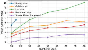
Fig. 3: Mean minimum number of ABSs required to provide a minimum rate of ${\color[rgb]{0,0,0}{\color[rgb]{0,0,0}r}}_{\text{min}}=5$ Mb/s vs. the number of GTs ($0pt=53$ m, $20\times 30\times 5$ SLF grid, $9\times 9\times 3$ fly grid).

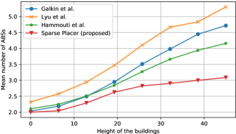
Fig. 4: Mean minimum number of ABSs required to provide a minimum rate of ${\color[rgb]{0,0,0}{\color[rgb]{0,0,0}r}}_{\text{min}}=20$ Mb/s vs. $0pt$ [m] ($20\times 30\times 150$ SLF grid, $9\times 9\times 5$ fly grid).

The area of interest is a rectangle of $500\times 400$ m with 9 streets in each direction delimited by 8 rows and columns of buildings of a certain height $0pt$. The flight height is between 50 and 150 m. The SLF is such that the absorption inside the buildings is 3 dB/m. The carrier frequency is 2.4 GHz, the bandwidth ${\color[rgb]{0,0,0}W}=20$ MHz, the transmit power ${\color[rgb]{0,0,0}P_{\text{TX}}}=0.1$ Watt, and the noise power ${\color[rgb]{0,0,0}\sigma^{2}}=-96$ dBm. A total of ${{\color[rgb]{0,0,0}M}}$ GTs are deployed on the street uniformly at random. The proposed algorithm is compared with the algorithm by Huang et al. [27], the K-means algorithm by Galkin et al. [28], the spiral-based algorithm by Lyu et al. [29], and the iterative algorithm by Hammouti et al. [11] for unlimited backhaul. The implementation of the algorithm in [27] was provided by the authors, whereas the rest were implemented by us. The algorithm in [27] is only used in one experiment since its computational complexity of $\mathcal{O}({{\color[rgb]{0,0,0}M}}^{6})$ makes it only suitable for a relatively low ${{\color[rgb]{0,0,0}M}}$. The positions returned by these algorithms are projected onto the grid ${{\color[rgb]{0,0,0}\bar{\mathcal{F}}}}$ of allowed flying positions.

The adopted performance metric is the minimum number of ABSs required to guarantee a rate ${\color[rgb]{0,0,0}{\color[rgb]{0,0,0}r}}_{\text{min}}$ to all GTs. This metric is averaged using Monte Carlo across realizations of the user locations. For the algorithms in [27] and [29], which are based on a maximum radius, the latter is gradually decreased starting from its value corresponding to free space propagation until all GTs receive the minimum rate. For the algorithms in [11] and [28], the number of centroids is gradually increased starting from 1 until the aforementioned rate condition is met. See the repository (link on the first page) for more details along with the code of all experiments.

Fig. 3 depicts the minimum number of ABSs required to guarantee a rate of ${\color[rgb]{0,0,0}{\color[rgb]{0,0,0}r}}_{\text{min}}=5$ Mb/s for all GTs. The proposed algorithm is seen to yield placements that require fewer ABSs than all competing algorithms. This can be ascribed to the fact that it is aware of the channel and of in which regions it is allowed to fly. To investigate further the impact of the former effect, Fig. 4 studies the influence of shadowing. For a building height $0pt=0$, propagation occurs in free space, which leads to all algorithms performing similarly. The slightly worse performance of the algorithm by Lyu et al. is mainly caused by the flight grid discretization. As $0pt$ increases, the channel gradually differs more and more from free-space propagation and the competing algorithms suffer a performance degradation.

Finally, Fig. 5 investigates the influence of ${\color[rgb]{0,0,0}{\color[rgb]{0,0,0}r}}_{\text{min}}$. It is seen that the sensitivity of the proposed algorithm is much smaller than the one of its competitors, for which the performance metric increases considerably as ${\color[rgb]{0,0,0}{\color[rgb]{0,0,0}r}}_{\text{min}}$ increases.

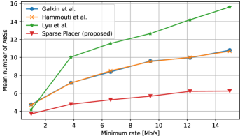
Fig. 5: Mean minimum number of ABSs required to provide a minimum rate of ${\color[rgb]{0,0,0}{\color[rgb]{0,0,0}r}}_{\text{min}}$ ($0pt=53$ m, $48\times 40\times 5$ SLF grid, $9\times 9\times 5$ fly grid).

6 Related Work

The most related works are [15, 30, 27]. In [15], a terrain map or 3D model of the environment is used to predict the channel. Unfortunately, such models are seldom available and, furthermore, their resolution is typically very low relative to typical wavelengths, which indicates that the resulting accuracy may be insufficient for placement purposes. Besides, a reinforcement learning approach is used rather than a convex optimization approach as in the present paper. The algorithm needs to be retrained in every new environment or if the number of UAVs changes. Besides, this approach is not flexible enough to accommodate additional constraints, for example that a human user must take control of one of the UAVs.

The approach in [30] relies on average local descriptors of the channel in terms of a map that provides the path loss exponent of each region in the deployment scenario. However, it just applies for ${{\color[rgb]{0,0,0}N}}={{\color[rgb]{0,0,0}M}}=1$.

Finally, [27] also adopts a convex optimization approach based on promoting sparsity, but the formulation is entirely different as it is not based on a discretization. Its complexity is $\mathcal{O}({{\color[rgb]{0,0,0}M}}^{6})$, which restricts its applicability to scenarios with a low number of GTs. Besides, it cannot accommodate general flight constraints since convexity would be lost in that case.

7 Conclusions

This paper proposes a new approach to ABS placement where, instead of relying on average characterizations of the channel, a radio map of the specific deployment scenario is constructed and used to determine the set of optimal ABS locations in terms of a convex objective that approximately minimizes the number of ABSs to guarantee a minimum rate to all GTs. Unlike most approaches, the proposed algorithm has a low complexity and can accommodate flight constraints such as no-fly zones or airspace occupied by buildings. The intuitive soundness of the scheme is empirically corroborated using an open source simulator developed in this work.

8 Supplementary Material

8.1 Notation

$\mathbb{R}_{++}$ is the set of positive real numbers. If $\bm{a}$ and $\bm{b}$ are vectors of the same dimension, then $\bm{a}\odot\bm{b}$ is the entrywise product of $\bm{a}$ and $\bm{b}$, whereas $\bm{a}\div\bm{b}$ is the entrywise quotient of $\bm{a}$ and $\bm{b}$.

8.2 An Algorithm for Air-to-ground Radio Tomography

As indicated in Sec. 3, the usual approximation to (4) using a weight function is not suitable to construct an air-to-ground radio map for ABS placement. Instead, this work proposes adopting a different approximation to the integral in (4). The technique, commonly used in other disciplines (see references in [23]) and hinted in a different context in [21], involves splitting the 3D space in voxels centered at the grid points ${{\color[rgb]{0,0,0}\bar{\mathcal{X}}}}:=\{{{\color[rgb]{0,0,0}\bm{x}}}^{{\color[rgb]{0,0,0}\bar{\mathcal{X}}}}_{1},\ldots,{{\color[rgb]{0,0,0}\bm{x}}}^{{\color[rgb]{0,0,0}\bar{\mathcal{X}}}}_{{\color[rgb]{0,0,0}Q}}\}$ and approximating ${\color[rgb]{0,0,0}l}$ by a function that takes the value ${\color[rgb]{0,0,0}l}({{\color[rgb]{0,0,0}\bm{x}}}^{{\color[rgb]{0,0,0}\bar{\mathcal{X}}}}_{{\color[rgb]{0,0,0}q}})$ at all points of the ${{\color[rgb]{0,0,0}q}}$-th voxel. The resulting piecewise constant approximation of ${\color[rgb]{0,0,0}l}$ can be integrated by determining the positions of the crossings between the voxel boundaries and the line segment between ${{\color[rgb]{0,0,0}\bm{{{\color[rgb]{0,0,0}x}}}}}_{1}$ and ${{\color[rgb]{0,0,0}\bm{{{\color[rgb]{0,0,0}x}}}}}_{2}$; see Fig. 2.

Algorithm 2, which can be classified as a parametric, floating point, and zeroth-order algorithm [23, Sec. I-B-1], is our implementation of the aforementioned approximation, yet others are possible. The idea is to parameterize the line segment between ${{\color[rgb]{0,0,0}\bm{{{\color[rgb]{0,0,0}x}}}}}_{1}$ and ${{\color[rgb]{0,0,0}\bm{{{\color[rgb]{0,0,0}x}}}}}_{2}$ as ${{\color[rgb]{0,0,0}\bm{{{\color[rgb]{0,0,0}x}}}}}(t)={{\color[rgb]{0,0,0}\bm{{{\color[rgb]{0,0,0}x}}}}}_{1}+t({{\color[rgb]{0,0,0}\bm{{{\color[rgb]{0,0,0}x}}}}}_{2}-{{\color[rgb]{0,0,0}\bm{{{\color[rgb]{0,0,0}x}}}}}_{1})$, where $t\in[0,1]$, and identify the values $t_{1},t_{2},\ldots,t_{T}$ for which the boundary between two adjacent voxels is crossed. Since $\|{{\color[rgb]{0,0,0}\bm{{{\color[rgb]{0,0,0}x}}}}}(t_{i})-{{\color[rgb]{0,0,0}\bm{{{\color[rgb]{0,0,0}x}}}}}(t_{i-1})\|=(t_{i}-t_{i-1})\|{{\color[rgb]{0,0,0}\bm{{{\color[rgb]{0,0,0}x}}}}}_{2}-{{\color[rgb]{0,0,0}\bm{{{\color[rgb]{0,0,0}x}}}}}_{1}\|$ whenever $t_{i}>t_{i-1}$, the approximation is then

$${\color[rgb]{0,0,0}\xi}({{\color[rgb]{0,0,0}\bm{{{\color[rgb]{0,0,0}x}}}}}_{1},{{\color[rgb]{0,0,0}\bm{{{\color[rgb]{0,0,0}x}}}}}_{2}) \approx\frac{\sum_{i=2}^{T}(t_{i}-t_{i-1})\|{{\color[rgb]{0,0,0}\bm{{{\color[rgb]{0,0,0}x}}}}}_{2}-{{\color[rgb]{0,0,0}\bm{{{\color[rgb]{0,0,0}x}}}}}_{1}\|{\color[rgb]{0,0,0}l}({{\color[rgb]{0,0,0}\bm{x}}}^{{\color[rgb]{0,0,0}\bar{\mathcal{X}}}}_{{{\color[rgb]{0,0,0}q}}_{i}})}{\|{{\color[rgb]{0,0,0}\bm{{{\color[rgb]{0,0,0}x}}}}}_{2}-{{\color[rgb]{0,0,0}\bm{{{\color[rgb]{0,0,0}x}}}}}_{1}\|^{1/2}}$$ (8)

$$=\|{{\color[rgb]{0,0,0}\bm{{{\color[rgb]{0,0,0}x}}}}}_{2}-{{\color[rgb]{0,0,0}\bm{{{\color[rgb]{0,0,0}x}}}}}_{1}\|^{1/2}\sum_{i=2}^{T}(t_{i}-t_{i-1}){\color[rgb]{0,0,0}l}({{\color[rgb]{0,0,0}\bm{x}}}^{{\color[rgb]{0,0,0}\bar{\mathcal{X}}}}_{{{\color[rgb]{0,0,0}q}}_{i}}),$$ (9)

where ${{{\color[rgb]{0,0,0}q}}_{i}}$ is the index of the $i$-th voxel crossed by the segment. Since ${{\color[rgb]{0,0,0}\bar{\mathcal{X}}}}$ is a 3D grid, each point in $\{{{\color[rgb]{0,0,0}\bm{x}}}^{{\color[rgb]{0,0,0}\bar{\mathcal{X}}}}_{1},\ldots,{{\color[rgb]{0,0,0}\bm{x}}}^{{\color[rgb]{0,0,0}\bar{\mathcal{X}}}}_{{\color[rgb]{0,0,0}Q}}\}$ can also be indexed by a vector ${\color[rgb]{0,0,0}\bm{i}}$ of 3 indices that lies in the set ${\color[rgb]{0,0,0}\mathcal{I}}:=\{1,\ldots,{{\color[rgb]{0,0,0}{{\color[rgb]{0,0,0}Q}}}}_{x}\}\times\{1,\ldots,{{\color[rgb]{0,0,0}{{\color[rgb]{0,0,0}Q}}}}_{y}\}\times\{1,\ldots,{{\color[rgb]{0,0,0}{{\color[rgb]{0,0,0}Q}}}}_{z}\}$. The values of the SLF can also be collected in a tensor ${\color[rgb]{0,0,0}\bm{{\color[rgb]{0,0,0}L}}}\in\mathbb{R}^{{{\color[rgb]{0,0,0}{{\color[rgb]{0,0,0}Q}}}}_{x}\times{{\color[rgb]{0,0,0}{{\color[rgb]{0,0,0}Q}}}}_{y}\times{{\color[rgb]{0,0,0}{{\color[rgb]{0,0,0}Q}}}}_{z}}$, whose entry ${\color[rgb]{0,0,0}L}[{\color[rgb]{0,0,0}\bm{i}}]$ is the value of ${\color[rgb]{0,0,0}l}$ at the ${\color[rgb]{0,0,0}\bm{i}}$-th grid point. If ${\color[rgb]{0,0,0}\bm{\delta}}_{{{\color[rgb]{0,0,0}\bar{\mathcal{X}}}}}\in\mathbb{R}_{++}^{3}$ denotes a vector whose $j$-th entry ${\color[rgb]{0,0,0}\delta}_{{{\color[rgb]{0,0,0}\bar{\mathcal{X}}}}}[j]$ represents the spacing between grid points along the $j$-th axis, the coordinates of the ${\color[rgb]{0,0,0}\bm{i}}$-th grid point are clearly ${\color[rgb]{0,0,0}\bm{i}}\odot{\color[rgb]{0,0,0}\bm{\delta}}_{{{\color[rgb]{0,0,0}\bar{\mathcal{X}}}}}$, where $\odot$ denotes entrywise product. Similarly, the boundaries between adjacent voxels along the $j$-th axis occur at values of the $j$-th coordinate given by ${\color[rgb]{0,0,0}\delta}_{{{\color[rgb]{0,0,0}\bar{\mathcal{X}}}}}[j]({\color[rgb]{0,0,0}i}\pm 1/2)$, where ${\color[rgb]{0,0,0}i}$ is an integer. It is then clear that steps 6-8 in Algorithm 2 simply find the next value of $t$ for which the segment crosses a voxel boundary along one of the axes by solving the equation

$${{\color[rgb]{0,0,0}x}}_{1}[j]+t({{\color[rgb]{0,0,0}x}}_{2}[j]-{{\color[rgb]{0,0,0}x}}_{1}[j])={\color[rgb]{0,0,0}\delta}_{{{\color[rgb]{0,0,0}\bar{\mathcal{X}}}}}[j]({\color[rgb]{0,0,0}i}_{\text{current}}[j]\pm{1}/{2})$$ (10)

for $t$ along each axis $j$ and taking the minimum across axes. The $\pm$ becomes a plus sign for the $j$-th axis if the segment is increasing along this axis and a minus sign otherwise.

An alternative implementation of the same integral approximation with smaller computational complexity but greater memory complexity could be obtained by creating 3 lists corresponding to the values of $t$ for which the line segment between ${{\color[rgb]{0,0,0}\bm{{{\color[rgb]{0,0,0}x}}}}}_{1}$ and ${{\color[rgb]{0,0,0}\bm{{{\color[rgb]{0,0,0}x}}}}}_{2}$ intersects each axis and then merging those lists into a list with non-decreasing values of $t$.

Algorithm 2 solves the limitations of the conventional approximation outlined in Sec. 3. First, Algorithm 2 yields an approximation of ${\color[rgb]{0,0,0}\xi}({{\color[rgb]{0,0,0}\bm{{{\color[rgb]{0,0,0}x}}}}}_{1},{{\color[rgb]{0,0,0}\bm{{{\color[rgb]{0,0,0}x}}}}}_{2})$ that is a continuous function of ${{\color[rgb]{0,0,0}\bm{{{\color[rgb]{0,0,0}x}}}}}_{1}$ and ${{\color[rgb]{0,0,0}\bm{{{\color[rgb]{0,0,0}x}}}}}_{2}$ since the line integral of a piecewise constant function is continuous. Besides, the issue of the approximation becoming zero when the ellipses in the right side of Fig. 2 miss all grid points disappears. For this reason, the voxels can now be kept large regardless of the wavelength and, therefore, the total number of voxels can be kept low enough to be handled given the available computational resources. Finally, as indicated in Sec. 3, the computational complexity of Algorithm 2 is much smaller than the one of the conventional approximation. Specifically, one can observe in Algorithm 2 that a constant number of products and additions are required for each crossing. The total number of crossings is at most ${{\color[rgb]{0,0,0}{{\color[rgb]{0,0,0}Q}}}}_{z}+{{\color[rgb]{0,0,0}{{\color[rgb]{0,0,0}Q}}}}_{y}+{{\color[rgb]{0,0,0}{{\color[rgb]{0,0,0}Q}}}}_{z}$, which means that, if ${{\color[rgb]{0,0,0}{{\color[rgb]{0,0,0}Q}}}}_{x}={{\color[rgb]{0,0,0}{{\color[rgb]{0,0,0}Q}}}}_{y}={{\color[rgb]{0,0,0}{{\color[rgb]{0,0,0}Q}}}}_{z}={{\color[rgb]{0,0,0}{{\color[rgb]{0,0,0}Q}}}}_{0}$, then the total complexity of Algorithm 2 is $\mathcal{O}({{\color[rgb]{0,0,0}{{\color[rgb]{0,0,0}Q}}}}_{0})$, whereas the complexity of the standard approximation is $\mathcal{O}({{\color[rgb]{0,0,0}{{\color[rgb]{0,0,0}Q}}}}_{0}^{3})$.

11:  Input: ${{\color[rgb]{0,0,0}\bm{{{\color[rgb]{0,0,0}x}}}}}_{1}$, ${{\color[rgb]{0,0,0}\bm{{{\color[rgb]{0,0,0}x}}}}}_{2}$, grid spacing vector ${\color[rgb]{0,0,0}\bm{\delta}}_{{{\color[rgb]{0,0,0}\bar{\mathcal{X}}}}}\in\mathbb{R}^{3}$,     SLF tensor ${\color[rgb]{0,0,0}\bm{{\color[rgb]{0,0,0}L}}}\in\mathbb{R}^{{{\color[rgb]{0,0,0}{{\color[rgb]{0,0,0}Q}}}}_{x}\times{{\color[rgb]{0,0,0}{{\color[rgb]{0,0,0}Q}}}}_{y}\times{{\color[rgb]{0,0,0}{{\color[rgb]{0,0,0}Q}}}}_{z}}$. 2:  Initialize ${\color[rgb]{0,0,0}\bm{\Delta}}_{{{\color[rgb]{0,0,0}\bm{{{\color[rgb]{0,0,0}x}}}}}}={{\color[rgb]{0,0,0}\bm{{{\color[rgb]{0,0,0}x}}}}}_{2}-{{\color[rgb]{0,0,0}\bm{{{\color[rgb]{0,0,0}x}}}}}_{1}$, ${\color[rgb]{0,0,0}\bm{b}}_{\text{inc}}=\mathop{\rm sign}({\color[rgb]{0,0,0}\bm{\Delta}}_{{{\color[rgb]{0,0,0}\bm{{{\color[rgb]{0,0,0}x}}}}}})$, ${\color[rgb]{0,0,0}{I}}=0$ 3:  Set zero entries of ${\color[rgb]{0,0,0}\bm{\Delta}}_{{{\color[rgb]{0,0,0}\bm{{{\color[rgb]{0,0,0}x}}}}}}$ to 1 # To avoid dividing by 0 4:  Set ${\color[rgb]{0,0,0}\bm{i}}_{\text{current}}=\text{round}({{\color[rgb]{0,0,0}\bm{{{\color[rgb]{0,0,0}x}}}}}_{1}\div{\color[rgb]{0,0,0}\bm{\delta}}_{{{\color[rgb]{0,0,0}\bar{\mathcal{X}}}}})$ # Index of current voxel 25:  while $t<1$ do 36:     Set ${\color[rgb]{0,0,0}\bm{t}}_{\text{cand}}=({\color[rgb]{0,0,0}\bm{\delta}}_{{{\color[rgb]{0,0,0}\bar{\mathcal{X}}}}}\odot({\color[rgb]{0,0,0}\bm{i}}_{\text{current}}+{\color[rgb]{0,0,0}\bm{b}}_{\text{inc}}/2)-{{\color[rgb]{0,0,0}\bm{{{\color[rgb]{0,0,0}x}}}}}_{1})\div{\color[rgb]{0,0,0}\bm{\Delta}}_{{{\color[rgb]{0,0,0}\bm{{{\color[rgb]{0,0,0}x}}}}}}$ 47:     Set ${\color[rgb]{0,0,0}i}_{\text{next}}=\operatorname*{arg\,min}_{i}{\color[rgb]{0,0,0}t}_{\text{cand}}[i]~{}\mathop{\text{s.t.}}~{}{\color[rgb]{0,0,0}b}_{\text{inc}}[i]\neq 0$ 58:     Set ${\color[rgb]{0,0,0}t}_{\text{next}}={\color[rgb]{0,0,0}t}_{\text{cand}}[{\color[rgb]{0,0,0}i}_{\text{next}}]$ 69:     Set ${\color[rgb]{0,0,0}{I}}={\color[rgb]{0,0,0}{I}}+(t-{\color[rgb]{0,0,0}t}_{\text{next}}){\color[rgb]{0,0,0}L}[{\color[rgb]{0,0,0}\bm{i}}_{\text{current}}]$ 710:     Set $t={\color[rgb]{0,0,0}t}_{\text{next}}$ 811:     Set ${\color[rgb]{0,0,0}\bm{i}}_{\text{current}}[{\color[rgb]{0,0,0}i}_{\text{next}}]={\color[rgb]{0,0,0}\bm{i}}_{\text{current}}[{\color[rgb]{0,0,0}i}_{\text{next}}]+{\color[rgb]{0,0,0}b}_{\text{inc}}[{\color[rgb]{0,0,0}i}_{\text{next}}]$ 12:  end while 13:  return $\|{{\color[rgb]{0,0,0}\bm{{{\color[rgb]{0,0,0}x}}}}}_{2}-{{\color[rgb]{0,0,0}\bm{{{\color[rgb]{0,0,0}x}}}}}_{1}\|^{1/2}{\color[rgb]{0,0,0}{I}}$

Algorithm 2 Tomographic Integral Approximation

8.3 Interior-Point Solver

This section details how an interior-point solver can be used to solve a relaxed version of (5).

Indeed, Problem (5) is non-convex due to the constraint ${\color[rgb]{0,0,0}\bm{\alpha}}\in\{0,1\}^{{{\color[rgb]{0,0,0}G}}}$. As pointed out in Sec. 4, a brute-force approach is not viable since ${{\color[rgb]{0,0,0}G}}$ will typically be large in real applications. Instead, it is more convenient to adopt a convex approximation by relaxing this constraint. This yields

$$\mathop{\text{minimize}}_{{\color[rgb]{0,0,0}\bm{\alpha}}\in[0,1]^{{{\color[rgb]{0,0,0}G}}}}\quad \|{\color[rgb]{0,0,0}\bm{\alpha}}\|_{0}$$ (11a)

$$\mathop{\text{s.t.}}\quad {\color[rgb]{0,0,0}\bm{C}}{\color[rgb]{0,0,0}\bm{\alpha}}\geq{\color[rgb]{0,0,0}{\color[rgb]{0,0,0}r}}_{\text{min}}\bm{1}$$ (11b)

where ${\color[rgb]{0,0,0}\bm{\alpha}}:=[{\color[rgb]{0,0,0}\alpha}_{1},\ldots,{\color[rgb]{0,0,0}\alpha}_{{\color[rgb]{0,0,0}G}}]^{\top}$ and ${\color[rgb]{0,0,0}\bm{C}}:=[{\color[rgb]{0,0,0}\bm{{\color[rgb]{0,0,0}c}}}_{1},\ldots,{\color[rgb]{0,0,0}\bm{{\color[rgb]{0,0,0}c}}}_{{\color[rgb]{0,0,0}G}}]$. Although it can be easily seen that this relaxation does not entail loss of optimality, the objective now is non-convex. As usual, this zero norm can be replaced with an $\ell_{1}$-norm to yield a convex problem:

$$\mathop{\text{minimize}}_{{\color[rgb]{0,0,0}\bm{\alpha}}\in[0,1]^{{{\color[rgb]{0,0,0}G}}}}\quad \|{\color[rgb]{0,0,0}\bm{\alpha}}\|_{1}$$ (12a)

$$\mathop{\text{s.t.}}\quad {\color[rgb]{0,0,0}\bm{C}}{\color[rgb]{0,0,0}\bm{\alpha}}\geq{\color[rgb]{0,0,0}{\color[rgb]{0,0,0}r}}_{\text{min}}\bm{1}.$$ (12b)

It is well-known though that the sparsity of the solutions can be increased by means of reweighting [26]. To this end, $\|{\color[rgb]{0,0,0}\bm{\alpha}}\|_{1}=\sum_{{\color[rgb]{0,0,0}g}}|{\color[rgb]{0,0,0}\alpha}_{{\color[rgb]{0,0,0}g}}|=\sum_{{\color[rgb]{0,0,0}g}}{\color[rgb]{0,0,0}\alpha}_{{\color[rgb]{0,0,0}g}}$ can be replaced with $\sum_{{\color[rgb]{0,0,0}g}}{\color[rgb]{0,0,0}w}_{{\color[rgb]{0,0,0}g}}{\color[rgb]{0,0,0}\alpha}_{{\color[rgb]{0,0,0}g}}$, where ${\color[rgb]{0,0,0}w}_{{\color[rgb]{0,0,0}g}}\geq 0$ are properly selected weights:

$$\mathop{\text{minimize}}_{{\color[rgb]{0,0,0}\bm{\alpha}}\in[0,1]^{{{\color[rgb]{0,0,0}G}}}}\quad {\color[rgb]{0,0,0}\bm{{\color[rgb]{0,0,0}w}}}^{\top}{\color[rgb]{0,0,0}\bm{\alpha}}$$ (13a)

$$\mathop{\text{s.t.}}\quad {\color[rgb]{0,0,0}\bm{C}}{\color[rgb]{0,0,0}\bm{\alpha}}\geq{\color[rgb]{0,0,0}{\color[rgb]{0,0,0}r}}_{\text{min}}\bm{1}$$ (13b)

The standard approach is to iteratively set ${\color[rgb]{0,0,0}w}_{{\color[rgb]{0,0,0}g}}=1/(\epsilon+{\color[rgb]{0,0,0}\tilde{\alpha}}_{{\color[rgb]{0,0,0}g}})$, where $\epsilon$ is a small constant and $\{{\color[rgb]{0,0,0}\tilde{\alpha}}_{{\color[rgb]{0,0,0}g}}\}_{{\color[rgb]{0,0,0}g}}$ are obtained by first solving the problem with a previous set of weights, the initial set being such that ${\color[rgb]{0,0,0}w}_{{\color[rgb]{0,0,0}g}}=1~{}\forall{{\color[rgb]{0,0,0}g}}$.

To apply an interior point solver, the inequality constraints can be replaced with equality constraints by introducing the vector of slack variables ${\color[rgb]{0,0,0}\bm{{\color[rgb]{0,0,0}s}}}$:

$$\mathop{\text{minimize}}_{{\color[rgb]{0,0,0}\bm{\alpha}}\in[0,1]^{{{\color[rgb]{0,0,0}G}}}}\quad {\color[rgb]{0,0,0}\bm{{\color[rgb]{0,0,0}w}}}^{\top}{\color[rgb]{0,0,0}\bm{\alpha}}$$ (14a)

$$\mathop{\text{s.t.}}\quad {\color[rgb]{0,0,0}\bm{C}}{\color[rgb]{0,0,0}\bm{\alpha}}={\color[rgb]{0,0,0}{\color[rgb]{0,0,0}r}}_{\text{min}}\bm{1}+{\color[rgb]{0,0,0}\bm{{\color[rgb]{0,0,0}s}}}$$ (14b)

$${\color[rgb]{0,0,0}\bm{{\color[rgb]{0,0,0}s}}}\geq\bm{0}$$ (14c)

Given that this problem has ${{\color[rgb]{0,0,0}G}}+{{\color[rgb]{0,0,0}M}}$ variables plus ${{\color[rgb]{0,0,0}M}}$ Lagrange multipliers associated with the equality constraints, each inner step of the interior point solver involves solving a system of ${{\color[rgb]{0,0,0}G}}+2{{\color[rgb]{0,0,0}M}}$ linear equations with ${{\color[rgb]{0,0,0}G}}+2{{\color[rgb]{0,0,0}M}}$ variables, which has a complexity $\mathcal{O}(({{\color[rgb]{0,0,0}G}}+2{{\color[rgb]{0,0,0}M}})^{3})$.

8.4 Derivation of Algorithm 1

The goal in this section is to derive a solver for (7) using the framework of ADMM [25].

To facilitate this task, it is convenient at this point to replace the objective with a linear function $\sum_{{\color[rgb]{0,0,0}g}}{\color[rgb]{0,0,0}w}_{{\color[rgb]{0,0,0}g}}{\color[rgb]{0,0,0}s}_{{\color[rgb]{0,0,0}g}}$, where $\{{\color[rgb]{0,0,0}s}_{{\color[rgb]{0,0,0}g}}\}_{{\color[rgb]{0,0,0}g}}$ are slack variables. Problem (7) can then be expressed as

$$\mathop{\text{minimize}}_{{\color[rgb]{0,0,0}\bm{R}}\in\mathbb{R}^{{{\color[rgb]{0,0,0}M}}\times{{\color[rgb]{0,0,0}G}}}}\quad {\color[rgb]{0,0,0}\bm{{\color[rgb]{0,0,0}w}}}^{\top}{\color[rgb]{0,0,0}\bm{{\color[rgb]{0,0,0}s}}}$$ (15a)

$$\mathop{\text{s.t.}}\quad {\color[rgb]{0,0,0}\bm{R}}\bm{1}={\color[rgb]{0,0,0}{\color[rgb]{0,0,0}r}}_{\text{min}}\bm{1}$$ (15b)

$$\bm{0}\leq{\color[rgb]{0,0,0}\bm{R}}\leq{\color[rgb]{0,0,0}\bm{C}}$$ (15c)

$${\color[rgb]{0,0,0}\bm{{\color[rgb]{0,0,0}r}}}_{{\color[rgb]{0,0,0}g}}\leq{\color[rgb]{0,0,0}s}_{{\color[rgb]{0,0,0}g}}\bm{1},~{}{{\color[rgb]{0,0,0}g}}=1,\ldots,{{\color[rgb]{0,0,0}G}},$$ (15d)

where ${\color[rgb]{0,0,0}\bm{{\color[rgb]{0,0,0}w}}}:=[{\color[rgb]{0,0,0}w}_{1},\ldots,{\color[rgb]{0,0,0}w}_{{\color[rgb]{0,0,0}G}}]^{\top}$ and ${\color[rgb]{0,0,0}\bm{{\color[rgb]{0,0,0}s}}}:=[{\color[rgb]{0,0,0}s}_{1},\ldots,{\color[rgb]{0,0,0}s}_{{\color[rgb]{0,0,0}G}}]^{\top}$.

The next step is to express (15) in form amenable to application of ADMM. For the problem at hand, notation can be simplified by adopting the following special homogeneous form:

$$\mathop{\text{minimize}}_{{{\color[rgb]{0,0,0}\bm{X}}},{{\color[rgb]{0,0,0}\bm{Z}}}}\quad {\color[rgb]{0,0,0}f}({{\color[rgb]{0,0,0}\bm{X}}})+{\color[rgb]{0,0,0}h}({{\color[rgb]{0,0,0}\bm{Z}}})$$ (16a)

$$\mathop{\text{s.t.}}\quad {{\color[rgb]{0,0,0}\bm{A}}}_{1}{{\color[rgb]{0,0,0}\bm{X}}}{{\color[rgb]{0,0,0}\bm{A}}}_{2}+{{\color[rgb]{0,0,0}\bm{B}}}_{1}{{\color[rgb]{0,0,0}\bm{Z}}}{{\color[rgb]{0,0,0}\bm{B}}}_{2}=\bm{0}.$$ (16b)

For this problem, the ADMM iteration from [25, Sec. 3.1.1] becomes

$${{\color[rgb]{0,0,0}\bm{X}}}^{{\color[rgb]{0,0,0}k}+1} =\operatorname*{arg\,min}_{{\color[rgb]{0,0,0}\bm{X}}}{\color[rgb]{0,0,0}f}({{\color[rgb]{0,0,0}\bm{X}}})+\frac{{\color[rgb]{0,0,0}\rho}}{2}\|{{\color[rgb]{0,0,0}\bm{A}}}_{1}{{\color[rgb]{0,0,0}\bm{X}}}{{\color[rgb]{0,0,0}\bm{A}}}_{2}+{{\color[rgb]{0,0,0}\bm{B}}}_{1}{{\color[rgb]{0,0,0}\bm{Z}}}^{{\color[rgb]{0,0,0}k}}{{\color[rgb]{0,0,0}\bm{B}}}_{2}+{{\color[rgb]{0,0,0}\bm{U}}}^{{\color[rgb]{0,0,0}k}}\|_{{\color[rgb]{0,0,0}\text{F}}}^{2}$$ (17a)

$${{\color[rgb]{0,0,0}\bm{Z}}}^{{\color[rgb]{0,0,0}k}+1} =\operatorname*{arg\,min}_{{\color[rgb]{0,0,0}\bm{Z}}}{\color[rgb]{0,0,0}h}({{\color[rgb]{0,0,0}\bm{Z}}})+\frac{{\color[rgb]{0,0,0}\rho}}{2}\|{{\color[rgb]{0,0,0}\bm{A}}}_{1}{{\color[rgb]{0,0,0}\bm{X}}}^{{\color[rgb]{0,0,0}k}+1}{{\color[rgb]{0,0,0}\bm{A}}}_{2}+{{\color[rgb]{0,0,0}\bm{B}}}_{1}{{\color[rgb]{0,0,0}\bm{Z}}}{{\color[rgb]{0,0,0}\bm{B}}}_{2}+{{\color[rgb]{0,0,0}\bm{U}}}^{{\color[rgb]{0,0,0}k}}\|_{{\color[rgb]{0,0,0}\text{F}}}^{2}$$ (17b)

$${{\color[rgb]{0,0,0}\bm{U}}}^{{\color[rgb]{0,0,0}k}+1} ={{\color[rgb]{0,0,0}\bm{U}}}^{{\color[rgb]{0,0,0}k}}+{{\color[rgb]{0,0,0}\bm{A}}}_{1}{{\color[rgb]{0,0,0}\bm{X}}}^{{\color[rgb]{0,0,0}k}+1}{{\color[rgb]{0,0,0}\bm{A}}}_{2}+{{\color[rgb]{0,0,0}\bm{B}}}_{1}{{\color[rgb]{0,0,0}\bm{Z}}}^{{\color[rgb]{0,0,0}k}+1}{{\color[rgb]{0,0,0}\bm{B}}}_{2},$$ (17c)

where ${{\color[rgb]{0,0,0}\bm{U}}}^{{\color[rgb]{0,0,0}k}}$ is a matrix of scaled dual variables and ${\color[rgb]{0,0,0}\rho}>0$ is the step-size parameter.

There are multiple possibilities to cast (15) as (16) and each one leads to updates of a different nature. Thus, several attempts are often required. As seen later, the following assignments yield suitable updates for the problem under consideration:

$${{\color[rgb]{0,0,0}\bm{X}}} \rightarrow[{\color[rgb]{0,0,0}\bm{R}}^{\top},{\color[rgb]{0,0,0}\bm{{\color[rgb]{0,0,0}s}}}]^{\top}$$ (18a)

$${{\color[rgb]{0,0,0}\bm{Z}}} \rightarrow{\color[rgb]{0,0,0}\bm{R}}$$ (18b)

$${\color[rgb]{0,0,0}f}({{\color[rgb]{0,0,0}\bm{X}}}) \rightarrow{\color[rgb]{0,0,0}\bm{{\color[rgb]{0,0,0}w}}}^{\top}{\color[rgb]{0,0,0}\bm{{\color[rgb]{0,0,0}s}}}+\sum_{{\color[rgb]{0,0,0}g}}\mathcal{I}[{\color[rgb]{0,0,0}\bm{{\color[rgb]{0,0,0}r}}}_{{\color[rgb]{0,0,0}g}}\leq{\color[rgb]{0,0,0}s}_{{\color[rgb]{0,0,0}g}}\bm{1}]$$ (18c)

$${\color[rgb]{0,0,0}h}({{\color[rgb]{0,0,0}\bm{X}}}) \rightarrow\mathcal{I}[{\color[rgb]{0,0,0}\bm{R}}\bm{1}={\color[rgb]{0,0,0}{\color[rgb]{0,0,0}r}}_{\text{min}}\bm{1}]+\mathcal{I}[\bm{0}\leq{\color[rgb]{0,0,0}\bm{R}}\leq{\color[rgb]{0,0,0}\bm{C}}]$$ (18d)

$${{\color[rgb]{0,0,0}\bm{A}}}_{1} \rightarrow[\bm{I}_{{\color[rgb]{0,0,0}M}},\bm{0}],~{}{{\color[rgb]{0,0,0}\bm{A}}}_{2}\rightarrow\bm{I}_{{{\color[rgb]{0,0,0}G}}},~{}{{\color[rgb]{0,0,0}\bm{B}}}_{1}\rightarrow-\bm{I}_{{\color[rgb]{0,0,0}M}},~{}{{\color[rgb]{0,0,0}\bm{B}}}_{2}\rightarrow\bm{I}_{{\color[rgb]{0,0,0}G}}.$$ (18e)

Here, $\mathcal{I}[\cdot]$ is a function that takes the value 0 when the condition inside brackets holds and $\infty$ otherwise. Note that with this choice for the matrices in (16), it follows that ${{\color[rgb]{0,0,0}\bm{A}}}_{1}{{\color[rgb]{0,0,0}\bm{X}}}{{\color[rgb]{0,0,0}\bm{A}}}_{2}+{{\color[rgb]{0,0,0}\bm{B}}}_{1}{{\color[rgb]{0,0,0}\bm{Z}}}{{\color[rgb]{0,0,0}\bm{B}}}_{2}={\color[rgb]{0,0,0}\bm{R}}-{{\color[rgb]{0,0,0}\bm{Z}}}$ and, therefore, the constraint in (16) imposes that ${\color[rgb]{0,0,0}\bm{R}}={{\color[rgb]{0,0,0}\bm{Z}}}$.

${{\color[rgb]{0,0,0}\bm{X}}}$-step. To derive the ${{\color[rgb]{0,0,0}\bm{X}}}$-update, observe that, with the above assignments, the problem in (17a) becomes

$$({\color[rgb]{0,0,0}\bm{R}}^{{\color[rgb]{0,0,0}k}+1},{\color[rgb]{0,0,0}\bm{{\color[rgb]{0,0,0}s}}}^{{\color[rgb]{0,0,0}k}+1})= \arg\min_{{\color[rgb]{0,0,0}\bm{R}},{\color[rgb]{0,0,0}\bm{{\color[rgb]{0,0,0}s}}}}~{}{\color[rgb]{0,0,0}\bm{{\color[rgb]{0,0,0}w}}}^{\top}{\color[rgb]{0,0,0}\bm{{\color[rgb]{0,0,0}s}}}+\sum_{{\color[rgb]{0,0,0}g}}\mathcal{I}[{\color[rgb]{0,0,0}\bm{{\color[rgb]{0,0,0}r}}}_{{\color[rgb]{0,0,0}g}}\leq{\color[rgb]{0,0,0}s}_{{\color[rgb]{0,0,0}g}}\bm{1}]$$

$$+\frac{{\color[rgb]{0,0,0}\rho}}{2}\|{\color[rgb]{0,0,0}\bm{R}}-{{\color[rgb]{0,0,0}\bm{Z}}}^{{\color[rgb]{0,0,0}k}}+{{\color[rgb]{0,0,0}\bm{U}}}^{{\color[rgb]{0,0,0}k}}\|_{{\color[rgb]{0,0,0}\text{F}}}^{2}$$ (19a)

$$= \arg\min_{{\color[rgb]{0,0,0}\bm{R}},{\color[rgb]{0,0,0}\bm{{\color[rgb]{0,0,0}s}}}}~{}\sum_{{\color[rgb]{0,0,0}g}}\big{[}{\color[rgb]{0,0,0}w}_{{\color[rgb]{0,0,0}g}}{\color[rgb]{0,0,0}s}_{{\color[rgb]{0,0,0}g}}+\mathcal{I}[{\color[rgb]{0,0,0}\bm{{\color[rgb]{0,0,0}r}}}_{{\color[rgb]{0,0,0}g}}\leq{\color[rgb]{0,0,0}s}_{{\color[rgb]{0,0,0}g}}\bm{1}]$$

$$+\frac{{\color[rgb]{0,0,0}\rho}}{2}\|{\color[rgb]{0,0,0}\bm{{\color[rgb]{0,0,0}r}}}_{{\color[rgb]{0,0,0}g}}-{{\color[rgb]{0,0,0}\bm{{{\color[rgb]{0,0,0}z}}}}}_{{\color[rgb]{0,0,0}g}}^{{\color[rgb]{0,0,0}k}}+{{\color[rgb]{0,0,0}\bm{{{\color[rgb]{0,0,0}u}}}}}_{{\color[rgb]{0,0,0}g}}^{{\color[rgb]{0,0,0}k}}\|_{2}^{2}\big{]},$$ (19b)

where ${{\color[rgb]{0,0,0}\bm{{{\color[rgb]{0,0,0}z}}}}}_{{\color[rgb]{0,0,0}g}}^{{\color[rgb]{0,0,0}k}}$ and ${{\color[rgb]{0,0,0}\bm{{{\color[rgb]{0,0,0}u}}}}}_{{\color[rgb]{0,0,0}g}}^{{\color[rgb]{0,0,0}k}}$ respectively denote the ${{\color[rgb]{0,0,0}g}}$-th column of ${{\color[rgb]{0,0,0}\bm{Z}}}^{{\color[rgb]{0,0,0}k}}$ and ${{\color[rgb]{0,0,0}\bm{U}}}^{{\color[rgb]{0,0,0}k}}$. This problem clearly separates into ${{\color[rgb]{0,0,0}G}}$ problems of the form

$$({\color[rgb]{0,0,0}\bm{{\color[rgb]{0,0,0}r}}}_{{\color[rgb]{0,0,0}g}}^{{\color[rgb]{0,0,0}k}+1},{\color[rgb]{0,0,0}s}_{{\color[rgb]{0,0,0}g}}^{{\color[rgb]{0,0,0}k}+1})=\arg\min_{{\color[rgb]{0,0,0}\bm{{\color[rgb]{0,0,0}r}}}_{{\color[rgb]{0,0,0}g}},{\color[rgb]{0,0,0}s}_{{\color[rgb]{0,0,0}g}}}~{} {\color[rgb]{0,0,0}w}_{{\color[rgb]{0,0,0}g}}{\color[rgb]{0,0,0}s}_{{\color[rgb]{0,0,0}g}}+\frac{{\color[rgb]{0,0,0}\rho}}{2}\|{\color[rgb]{0,0,0}\bm{{\color[rgb]{0,0,0}r}}}_{{\color[rgb]{0,0,0}g}}-{{\color[rgb]{0,0,0}\bm{{{\color[rgb]{0,0,0}z}}}}}_{{\color[rgb]{0,0,0}g}}^{{\color[rgb]{0,0,0}k}}+{{\color[rgb]{0,0,0}\bm{{{\color[rgb]{0,0,0}u}}}}}_{{\color[rgb]{0,0,0}g}}^{{\color[rgb]{0,0,0}k}}\|_{2}^{2}$$ (20a)

$$\mathop{\text{s.t.}}\quad {\color[rgb]{0,0,0}\bm{{\color[rgb]{0,0,0}r}}}_{{\color[rgb]{0,0,0}g}}\leq{\color[rgb]{0,0,0}s}_{{\color[rgb]{0,0,0}g}}\bm{1}.$$ (20b)

If ${\color[rgb]{0,0,0}w}_{{\color[rgb]{0,0,0}g}}=0$, the inequality constraint can be removed and the optimum is attained when ${\color[rgb]{0,0,0}\bm{{\color[rgb]{0,0,0}r}}}_{{\color[rgb]{0,0,0}g}}^{{\color[rgb]{0,0,0}k}+1}={{\color[rgb]{0,0,0}\bm{{{\color[rgb]{0,0,0}z}}}}}_{{\color[rgb]{0,0,0}g}}^{{\color[rgb]{0,0,0}k}}-{{\color[rgb]{0,0,0}\bm{{{\color[rgb]{0,0,0}u}}}}}_{{\color[rgb]{0,0,0}g}}^{{\color[rgb]{0,0,0}k}}$. Thus, it suffices to focus on the case ${\color[rgb]{0,0,0}w}_{{\color[rgb]{0,0,0}g}}>0$. In this case, we have the following:

Proposition 1

If ${\color[rgb]{0,0,0}w}_{{\color[rgb]{0,0,0}g}}>0$, then ${\color[rgb]{0,0,0}\bm{{\color[rgb]{0,0,0}r}}}_{{\color[rgb]{0,0,0}g}}^{{\color[rgb]{0,0,0}k}+1}$ and ${\color[rgb]{0,0,0}s}_{{\color[rgb]{0,0,0}g}}^{{\color[rgb]{0,0,0}k}+1}$ satisfy

$${\color[rgb]{0,0,0}\bm{{\color[rgb]{0,0,0}r}}}_{{\color[rgb]{0,0,0}g}}^{{\color[rgb]{0,0,0}k}+1}=\min({{\color[rgb]{0,0,0}\bm{{{\color[rgb]{0,0,0}z}}}}}_{{\color[rgb]{0,0,0}g}}^{{\color[rgb]{0,0,0}k}}-{{\color[rgb]{0,0,0}\bm{{{\color[rgb]{0,0,0}u}}}}}_{{\color[rgb]{0,0,0}g}}^{{\color[rgb]{0,0,0}k}},{\color[rgb]{0,0,0}s}_{{\color[rgb]{0,0,0}g}}^{{\color[rgb]{0,0,0}k}+1}\bm{1})$$ (21a)

$$\bm{1}^{\top}\max({{\color[rgb]{0,0,0}\bm{{{\color[rgb]{0,0,0}z}}}}}_{{\color[rgb]{0,0,0}g}}^{{\color[rgb]{0,0,0}k}}-{{\color[rgb]{0,0,0}\bm{{{\color[rgb]{0,0,0}u}}}}}_{{\color[rgb]{0,0,0}g}}^{{\color[rgb]{0,0,0}k}}-{\color[rgb]{0,0,0}s}_{{\color[rgb]{0,0,0}g}}^{{\color[rgb]{0,0,0}k}+1}\bm{1},\bm{0})=\frac{{\color[rgb]{0,0,0}w}_{{\color[rgb]{0,0,0}g}}}{{\color[rgb]{0,0,0}\rho}},$$ (21b)

where $\min$ and $\max$ operate entrywise.

Proof. Since Problem (20) is convex differentiable and Slater’s conditions are satisfied, it follows that the Karush-Kuhn-Tucker (KKT) conditions are sufficient and necessary. To obtain these conditions, observe that the Lagrangian of (20) is given by

$${{\color[rgb]{0,0,0}\mathcal{L}}}({\color[rgb]{0,0,0}\bm{{\color[rgb]{0,0,0}r}}}_{{\color[rgb]{0,0,0}g}},{\color[rgb]{0,0,0}s}_{{\color[rgb]{0,0,0}g}};{{\color[rgb]{0,0,0}\bm{{{\color[rgb]{0,0,0}\nu}}}}})={\color[rgb]{0,0,0}w}_{{\color[rgb]{0,0,0}g}}{\color[rgb]{0,0,0}s}_{{\color[rgb]{0,0,0}g}}+\frac{{\color[rgb]{0,0,0}\rho}}{2}\|{\color[rgb]{0,0,0}\bm{{\color[rgb]{0,0,0}r}}}_{{\color[rgb]{0,0,0}g}}-{{\color[rgb]{0,0,0}\bm{{{\color[rgb]{0,0,0}z}}}}}_{{\color[rgb]{0,0,0}g}}^{{\color[rgb]{0,0,0}k}}+{{\color[rgb]{0,0,0}\bm{{{\color[rgb]{0,0,0}u}}}}}_{{\color[rgb]{0,0,0}g}}^{{\color[rgb]{0,0,0}k}}\|_{2}^{2}+{{\color[rgb]{0,0,0}\bm{{{\color[rgb]{0,0,0}\nu}}}}}^{\top}({\color[rgb]{0,0,0}\bm{{\color[rgb]{0,0,0}r}}}_{{\color[rgb]{0,0,0}g}}-{\color[rgb]{0,0,0}s}_{{\color[rgb]{0,0,0}g}}\bm{1}).$$ (22)

The KKT conditions are, therefore,

$$\nabla_{{\color[rgb]{0,0,0}\bm{{\color[rgb]{0,0,0}r}}}_{{\color[rgb]{0,0,0}g}}}{{\color[rgb]{0,0,0}\mathcal{L}}}({\color[rgb]{0,0,0}\bm{{\color[rgb]{0,0,0}r}}}_{{\color[rgb]{0,0,0}g}},{\color[rgb]{0,0,0}s}_{{\color[rgb]{0,0,0}g}};{{\color[rgb]{0,0,0}\bm{{{\color[rgb]{0,0,0}\nu}}}}}) ={\color[rgb]{0,0,0}\rho}({\color[rgb]{0,0,0}\bm{{\color[rgb]{0,0,0}r}}}_{{\color[rgb]{0,0,0}g}}-{{\color[rgb]{0,0,0}\bm{{{\color[rgb]{0,0,0}z}}}}}_{{\color[rgb]{0,0,0}g}}^{{\color[rgb]{0,0,0}k}}+{{\color[rgb]{0,0,0}\bm{{{\color[rgb]{0,0,0}u}}}}}_{{\color[rgb]{0,0,0}g}}^{{\color[rgb]{0,0,0}k}})+{{\color[rgb]{0,0,0}\bm{{{\color[rgb]{0,0,0}\nu}}}}}=\bm{0}$$ (23a)

$$\nabla_{{\color[rgb]{0,0,0}s}_{{\color[rgb]{0,0,0}g}}}{{\color[rgb]{0,0,0}\mathcal{L}}}({\color[rgb]{0,0,0}\bm{{\color[rgb]{0,0,0}r}}}_{{\color[rgb]{0,0,0}g}},{\color[rgb]{0,0,0}s}_{{\color[rgb]{0,0,0}g}};{{\color[rgb]{0,0,0}\bm{{{\color[rgb]{0,0,0}\nu}}}}}) ={\color[rgb]{0,0,0}w}_{{\color[rgb]{0,0,0}g}}-\bm{1}^{\top}{{\color[rgb]{0,0,0}\bm{{{\color[rgb]{0,0,0}\nu}}}}}=0$$ (23b)

$${\color[rgb]{0,0,0}\bm{{\color[rgb]{0,0,0}r}}}_{{\color[rgb]{0,0,0}g}} \leq{\color[rgb]{0,0,0}s}_{{\color[rgb]{0,0,0}g}}\bm{1}$$ (23c)

$${{\color[rgb]{0,0,0}\bm{{{\color[rgb]{0,0,0}\nu}}}}} \geq\bm{0},~{}~{}{{\color[rgb]{0,0,0}\nu}}[{{\color[rgb]{0,0,0}m}}]({\color[rgb]{0,0,0}r}_{{\color[rgb]{0,0,0}g}}[{{\color[rgb]{0,0,0}m}}]-{\color[rgb]{0,0,0}s}_{{\color[rgb]{0,0,0}g}})=0~{}\forall{{\color[rgb]{0,0,0}m}}.$$ (23d)

From (23a) and the inequality in (23d), it follows that

$${{\color[rgb]{0,0,0}\bm{{{\color[rgb]{0,0,0}\nu}}}}}=-{\color[rgb]{0,0,0}\rho}({\color[rgb]{0,0,0}\bm{{\color[rgb]{0,0,0}r}}}_{{\color[rgb]{0,0,0}g}}-{{\color[rgb]{0,0,0}\bm{{{\color[rgb]{0,0,0}z}}}}}_{{\color[rgb]{0,0,0}g}}^{{\color[rgb]{0,0,0}k}}+{{\color[rgb]{0,0,0}\bm{{{\color[rgb]{0,0,0}u}}}}}_{{\color[rgb]{0,0,0}g}}^{{\color[rgb]{0,0,0}k}})\geq\bm{0}.$$ (24)

This implies that ${\color[rgb]{0,0,0}\bm{{\color[rgb]{0,0,0}r}}}_{{\color[rgb]{0,0,0}g}}\leq{{\color[rgb]{0,0,0}\bm{{{\color[rgb]{0,0,0}z}}}}}_{{\color[rgb]{0,0,0}g}}^{{\color[rgb]{0,0,0}k}}-{{\color[rgb]{0,0,0}\bm{{{\color[rgb]{0,0,0}u}}}}}_{{\color[rgb]{0,0,0}g}}^{{\color[rgb]{0,0,0}k}}$. Combining this inequality with (23c) yields

$${\color[rgb]{0,0,0}\bm{{\color[rgb]{0,0,0}r}}}_{{\color[rgb]{0,0,0}g}}\leq\min({{\color[rgb]{0,0,0}\bm{{{\color[rgb]{0,0,0}z}}}}}_{{\color[rgb]{0,0,0}g}}^{{\color[rgb]{0,0,0}k}}-{{\color[rgb]{0,0,0}\bm{{{\color[rgb]{0,0,0}u}}}}}_{{\color[rgb]{0,0,0}g}}^{{\color[rgb]{0,0,0}k}},{\color[rgb]{0,0,0}s}_{{\color[rgb]{0,0,0}g}}\bm{1}).$$ (25)

On the other hand, from the equality in (24) and the inequality in (23d), one finds that

$$-{\color[rgb]{0,0,0}\rho}({\color[rgb]{0,0,0}r}_{{\color[rgb]{0,0,0}g}}[{{\color[rgb]{0,0,0}m}}]-{{\color[rgb]{0,0,0}z}}_{{\color[rgb]{0,0,0}g}}^{{\color[rgb]{0,0,0}k}}[{{\color[rgb]{0,0,0}m}}]+{{\color[rgb]{0,0,0}u}}_{{\color[rgb]{0,0,0}g}}^{{\color[rgb]{0,0,0}k}}[{{\color[rgb]{0,0,0}m}}])({\color[rgb]{0,0,0}r}_{{\color[rgb]{0,0,0}g}}[{{\color[rgb]{0,0,0}m}}]-{\color[rgb]{0,0,0}s}_{{\color[rgb]{0,0,0}g}})=0~{}\forall{{\color[rgb]{0,0,0}m}}.$$ (26)

This holds if and only if either ${\color[rgb]{0,0,0}r}_{{\color[rgb]{0,0,0}g}}[{{\color[rgb]{0,0,0}m}}]={{\color[rgb]{0,0,0}z}}_{{\color[rgb]{0,0,0}g}}^{{\color[rgb]{0,0,0}k}}[{{\color[rgb]{0,0,0}m}}]-{{\color[rgb]{0,0,0}u}}_{{\color[rgb]{0,0,0}g}}^{{\color[rgb]{0,0,0}k}}[{{\color[rgb]{0,0,0}m}}]$ or ${\color[rgb]{0,0,0}r}_{{\color[rgb]{0,0,0}g}}[{{\color[rgb]{0,0,0}m}}]={\color[rgb]{0,0,0}s}_{{\color[rgb]{0,0,0}g}}$. Therefore, it follows from (25) that

$${\color[rgb]{0,0,0}\bm{{\color[rgb]{0,0,0}r}}}_{{\color[rgb]{0,0,0}g}}=\min({{\color[rgb]{0,0,0}\bm{{{\color[rgb]{0,0,0}z}}}}}_{{\color[rgb]{0,0,0}g}}^{{\color[rgb]{0,0,0}k}}-{{\color[rgb]{0,0,0}\bm{{{\color[rgb]{0,0,0}u}}}}}_{{\color[rgb]{0,0,0}g}}^{{\color[rgb]{0,0,0}k}},{\color[rgb]{0,0,0}s}_{{\color[rgb]{0,0,0}g}}\bm{1}),$$ (27)

which establishes (21a). Finally, combine this expression with (23b) and (24) to arrive at

$${\color[rgb]{0,0,0}w}_{{\color[rgb]{0,0,0}g}} =-{\color[rgb]{0,0,0}\rho}\bm{1}^{\top}({\color[rgb]{0,0,0}\bm{{\color[rgb]{0,0,0}r}}}_{{\color[rgb]{0,0,0}g}}-{{\color[rgb]{0,0,0}\bm{{{\color[rgb]{0,0,0}z}}}}}_{{\color[rgb]{0,0,0}g}}^{{\color[rgb]{0,0,0}k}}+{{\color[rgb]{0,0,0}\bm{{{\color[rgb]{0,0,0}u}}}}}_{{\color[rgb]{0,0,0}g}}^{{\color[rgb]{0,0,0}k}})$$ (28a)

$$=-{\color[rgb]{0,0,0}\rho}\bm{1}^{\top}(\min({{\color[rgb]{0,0,0}\bm{{{\color[rgb]{0,0,0}z}}}}}_{{\color[rgb]{0,0,0}g}}^{{\color[rgb]{0,0,0}k}}-{{\color[rgb]{0,0,0}\bm{{{\color[rgb]{0,0,0}u}}}}}_{{\color[rgb]{0,0,0}g}}^{{\color[rgb]{0,0,0}k}},{\color[rgb]{0,0,0}s}_{{\color[rgb]{0,0,0}g}}\bm{1})-{{\color[rgb]{0,0,0}\bm{{{\color[rgb]{0,0,0}z}}}}}_{{\color[rgb]{0,0,0}g}}^{{\color[rgb]{0,0,0}k}}+{{\color[rgb]{0,0,0}\bm{{{\color[rgb]{0,0,0}u}}}}}_{{\color[rgb]{0,0,0}g}}^{{\color[rgb]{0,0,0}k}})$$ (28b)

$$=-{\color[rgb]{0,0,0}\rho}\bm{1}^{\top}\min(\bm{0},{\color[rgb]{0,0,0}s}_{{\color[rgb]{0,0,0}g}}\bm{1}-{{\color[rgb]{0,0,0}\bm{{{\color[rgb]{0,0,0}z}}}}}_{{\color[rgb]{0,0,0}g}}^{{\color[rgb]{0,0,0}k}}+{{\color[rgb]{0,0,0}\bm{{{\color[rgb]{0,0,0}u}}}}}_{{\color[rgb]{0,0,0}g}}^{{\color[rgb]{0,0,0}k}})$$ (28c)

$$={\color[rgb]{0,0,0}\rho}\bm{1}^{\top}\max(\bm{0},{{\color[rgb]{0,0,0}\bm{{{\color[rgb]{0,0,0}z}}}}}_{{\color[rgb]{0,0,0}g}}^{{\color[rgb]{0,0,0}k}}-{{\color[rgb]{0,0,0}\bm{{{\color[rgb]{0,0,0}u}}}}}_{{\color[rgb]{0,0,0}g}}^{{\color[rgb]{0,0,0}k}}-{\color[rgb]{0,0,0}s}_{{\color[rgb]{0,0,0}g}}\bm{1}),$$ (28d)

thereby recovering (21b). The proof is complete by noting that (23) holds if and only if (27) and (28d) hold.

$\blacksquare$

Observe that (21a) can be used to obtain ${\color[rgb]{0,0,0}\bm{{\color[rgb]{0,0,0}r}}}_{{\color[rgb]{0,0,0}g}}^{{\color[rgb]{0,0,0}k}+1}$ if ${\color[rgb]{0,0,0}s}_{{\color[rgb]{0,0,0}g}}^{{\color[rgb]{0,0,0}k}+1}$ is given, whereas (21b) does not depend on ${\color[rgb]{0,0,0}\bm{{\color[rgb]{0,0,0}r}}}_{{\color[rgb]{0,0,0}g}}^{{\color[rgb]{0,0,0}k}+1}$. Therefore, a solution to (21) can be found by first solving (21b) for ${\color[rgb]{0,0,0}s}_{{\color[rgb]{0,0,0}g}}^{{\color[rgb]{0,0,0}k}+1}$ and then substituting the result into the right-hand side of (21a) to recover ${\color[rgb]{0,0,0}\bm{{\color[rgb]{0,0,0}r}}}_{{\color[rgb]{0,0,0}g}}^{{\color[rgb]{0,0,0}k}+1}$. To this end, we have the following:

Proposition 2

prop:rootssg Equation (21b) has a unique root. This root lies in the interval $[\check{\color[rgb]{0,0,0}s}_{{\color[rgb]{0,0,0}g}}^{{\color[rgb]{0,0,0}k}},\hat{\color[rgb]{0,0,0}s}_{{\color[rgb]{0,0,0}g}}^{{\color[rgb]{0,0,0}k}}]$, where

$$\check{\color[rgb]{0,0,0}s}_{{\color[rgb]{0,0,0}g}}^{{\color[rgb]{0,0,0}k}} :=\min_{{\color[rgb]{0,0,0}m}}\left({{\color[rgb]{0,0,0}z}}_{{\color[rgb]{0,0,0}g}}^{{\color[rgb]{0,0,0}k}}[{{\color[rgb]{0,0,0}m}}]-{{\color[rgb]{0,0,0}u}}_{{\color[rgb]{0,0,0}g}}^{{\color[rgb]{0,0,0}k}}[{{\color[rgb]{0,0,0}m}}]\right)-\frac{{\color[rgb]{0,0,0}w}_{{\color[rgb]{0,0,0}g}}}{{{\color[rgb]{0,0,0}M}}{\color[rgb]{0,0,0}\rho}}$$ (29a)

$$\hat{\color[rgb]{0,0,0}s}_{{\color[rgb]{0,0,0}g}}^{{\color[rgb]{0,0,0}k}} :=\max_{{\color[rgb]{0,0,0}m}}\left({{\color[rgb]{0,0,0}z}}_{{\color[rgb]{0,0,0}g}}^{{\color[rgb]{0,0,0}k}}[{{\color[rgb]{0,0,0}m}}]-{{\color[rgb]{0,0,0}u}}_{{\color[rgb]{0,0,0}g}}^{{\color[rgb]{0,0,0}k}}[{{\color[rgb]{0,0,0}m}}]\right)-\frac{{\color[rgb]{0,0,0}w}_{{\color[rgb]{0,0,0}g}}}{{{\color[rgb]{0,0,0}M}}{\color[rgb]{0,0,0}\rho}}.$$ (29b)

Proof. Consider the function ${{\color[rgb]{0,0,0}F}}({\color[rgb]{0,0,0}s}):=\bm{1}^{\top}\max({{\color[rgb]{0,0,0}z}}_{{\color[rgb]{0,0,0}g}}^{{\color[rgb]{0,0,0}k}}-{{\color[rgb]{0,0,0}u}}_{{\color[rgb]{0,0,0}g}}^{{\color[rgb]{0,0,0}k}}-{\color[rgb]{0,0,0}s}\bm{1},\bm{0})=\sum_{{\color[rgb]{0,0,0}m}}\max({{\color[rgb]{0,0,0}z}}_{{\color[rgb]{0,0,0}g}}^{{\color[rgb]{0,0,0}k}}[{{\color[rgb]{0,0,0}m}}]-{{\color[rgb]{0,0,0}u}}_{{\color[rgb]{0,0,0}g}}^{{\color[rgb]{0,0,0}k}}[{{\color[rgb]{0,0,0}m}}]-{\color[rgb]{0,0,0}s},\bm{0})$. Since ${{\color[rgb]{0,0,0}F}}$ is the sum of non-increasing piecewise linear functions, so is ${{\color[rgb]{0,0,0}F}}$. Since ${{\color[rgb]{0,0,0}F}}({\color[rgb]{0,0,0}s})\rightarrow\infty$ as ${\color[rgb]{0,0,0}s}\rightarrow-\infty$ and ${{\color[rgb]{0,0,0}F}}({\color[rgb]{0,0,0}s})=0$ for a sufficiently large ${\color[rgb]{0,0,0}s}$, it follows that (21b) has at least one root. Uniqueness of the root follows readily by noting that ${{\color[rgb]{0,0,0}F}}$ is strictly decreasing whenever ${{\color[rgb]{0,0,0}F}}({\color[rgb]{0,0,0}s})>0$.

It remains to be shown that ${{\color[rgb]{0,0,0}F}}(\check{\color[rgb]{0,0,0}s}_{{\color[rgb]{0,0,0}g}}^{{\color[rgb]{0,0,0}k}})\geq{{\color[rgb]{0,0,0}w}_{{\color[rgb]{0,0,0}g}}}/({{{\color[rgb]{0,0,0}M}}{\color[rgb]{0,0,0}\rho}})$ whereas ${{\color[rgb]{0,0,0}F}}(\hat{\color[rgb]{0,0,0}s}_{{\color[rgb]{0,0,0}g}}^{{\color[rgb]{0,0,0}k}})\leq{{\color[rgb]{0,0,0}w}_{{\color[rgb]{0,0,0}g}}}/({{{\color[rgb]{0,0,0}M}}{\color[rgb]{0,0,0}\rho}})$. For the first of these inequalities, observe that $\check{\color[rgb]{0,0,0}s}_{{\color[rgb]{0,0,0}g}}^{{\color[rgb]{0,0,0}k}}\leq{{\color[rgb]{0,0,0}z}}_{{\color[rgb]{0,0,0}g}}^{{\color[rgb]{0,0,0}k}}[{{\color[rgb]{0,0,0}m}}]-{{\color[rgb]{0,0,0}u}}_{{\color[rgb]{0,0,0}g}}^{{\color[rgb]{0,0,0}k}}[{{\color[rgb]{0,0,0}m}}]-{{\color[rgb]{0,0,0}w}_{{\color[rgb]{0,0,0}g}}}/({{{\color[rgb]{0,0,0}M}}{\color[rgb]{0,0,0}\rho}})$ for all ${{\color[rgb]{0,0,0}m}}$, which in turn implies that ${{\color[rgb]{0,0,0}z}}_{{\color[rgb]{0,0,0}g}}^{{\color[rgb]{0,0,0}k}}[{{\color[rgb]{0,0,0}m}}]-{{\color[rgb]{0,0,0}u}}_{{\color[rgb]{0,0,0}g}}^{{\color[rgb]{0,0,0}k}}[{{\color[rgb]{0,0,0}m}}]-\check{\color[rgb]{0,0,0}s}_{{\color[rgb]{0,0,0}g}}^{{\color[rgb]{0,0,0}k}}\geq{{\color[rgb]{0,0,0}w}_{{\color[rgb]{0,0,0}g}}}/({{{\color[rgb]{0,0,0}M}}{\color[rgb]{0,0,0}\rho}})$. Thus, $\max({{\color[rgb]{0,0,0}z}}_{{\color[rgb]{0,0,0}g}}^{{\color[rgb]{0,0,0}k}}[{{\color[rgb]{0,0,0}m}}]-{{\color[rgb]{0,0,0}u}}_{{\color[rgb]{0,0,0}g}}^{{\color[rgb]{0,0,0}k}}[{{\color[rgb]{0,0,0}m}}]-\check{\color[rgb]{0,0,0}s}_{{\color[rgb]{0,0,0}g}}^{{\color[rgb]{0,0,0}k}},0)={{\color[rgb]{0,0,0}z}}_{{\color[rgb]{0,0,0}g}}^{{\color[rgb]{0,0,0}k}}[{{\color[rgb]{0,0,0}m}}]-{{\color[rgb]{0,0,0}u}}_{{\color[rgb]{0,0,0}g}}^{{\color[rgb]{0,0,0}k}}[{{\color[rgb]{0,0,0}m}}]-\check{\color[rgb]{0,0,0}s}_{{\color[rgb]{0,0,0}g}}^{{\color[rgb]{0,0,0}k}}\geq{{\color[rgb]{0,0,0}w}_{{\color[rgb]{0,0,0}g}}}/({{{\color[rgb]{0,0,0}M}}{\color[rgb]{0,0,0}\rho}})$, which yields ${{\color[rgb]{0,0,0}F}}(\check{\color[rgb]{0,0,0}s}_{{\color[rgb]{0,0,0}g}}^{{\color[rgb]{0,0,0}k}})\geq\sum_{{\color[rgb]{0,0,0}m}}{{\color[rgb]{0,0,0}w}_{{\color[rgb]{0,0,0}g}}}/({{{\color[rgb]{0,0,0}M}}{\color[rgb]{0,0,0}\rho}})={{\color[rgb]{0,0,0}w}_{{\color[rgb]{0,0,0}g}}}/{{\color[rgb]{0,0,0}\rho}}$. For the second inequality, note similarly that ${{\color[rgb]{0,0,0}z}}_{{\color[rgb]{0,0,0}g}}^{{\color[rgb]{0,0,0}k}}[{{\color[rgb]{0,0,0}m}}]-{{\color[rgb]{0,0,0}u}}_{{\color[rgb]{0,0,0}g}}^{{\color[rgb]{0,0,0}k}}[{{\color[rgb]{0,0,0}m}}]-\hat{\color[rgb]{0,0,0}s}_{{\color[rgb]{0,0,0}g}}^{{\color[rgb]{0,0,0}k}}\leq{{\color[rgb]{0,0,0}w}_{{\color[rgb]{0,0,0}g}}}/({{{\color[rgb]{0,0,0}M}}{\color[rgb]{0,0,0}\rho}})$ for all ${{\color[rgb]{0,0,0}m}}$. This means that ${{\color[rgb]{0,0,0}F}}(\hat{\color[rgb]{0,0,0}s}_{{\color[rgb]{0,0,0}g}}^{{\color[rgb]{0,0,0}k}})\leq\sum_{{\color[rgb]{0,0,0}m}}\max({{\color[rgb]{0,0,0}w}_{{\color[rgb]{0,0,0}g}}}/({{{\color[rgb]{0,0,0}M}}{\color[rgb]{0,0,0}\rho}}),0)={{\color[rgb]{0,0,0}w}_{{\color[rgb]{0,0,0}g}}}/{{\color[rgb]{0,0,0}\rho}}$.

$\blacksquare$

${{\color[rgb]{0,0,0}\bm{Z}}}$-step. From (17b) and (18), it follows that

$${{\color[rgb]{0,0,0}\bm{Z}}}^{{\color[rgb]{0,0,0}k}+1}=\operatorname*{arg\,min}_{{\color[rgb]{0,0,0}\bm{Z}}}~{}~{} \bigg{[}\mathcal{I}[{{\color[rgb]{0,0,0}\bm{Z}}}\bm{1}={\color[rgb]{0,0,0}{\color[rgb]{0,0,0}r}}_{\text{min}}\bm{1}]+\mathcal{I}[\bm{0}\leq{{\color[rgb]{0,0,0}\bm{Z}}}\leq{\color[rgb]{0,0,0}\bm{C}}]$$ (30a)

$$+\frac{{\color[rgb]{0,0,0}\rho}}{2}\|{\color[rgb]{0,0,0}\bm{R}}^{{\color[rgb]{0,0,0}k}+1}-{{\color[rgb]{0,0,0}\bm{Z}}}+{{\color[rgb]{0,0,0}\bm{U}}}^{{\color[rgb]{0,0,0}k}}\|_{{\color[rgb]{0,0,0}\text{F}}}^{2}\bigg{]}$$ (30b)

$$=\operatorname*{arg\,min}_{{\color[rgb]{0,0,0}\bm{Z}}}~{}~{} \sum_{{\color[rgb]{0,0,0}m}}\bigg{[}\mathcal{I}[{{\color[rgb]{0,0,0}{\bar{\bm{z}}}}}_{{\color[rgb]{0,0,0}m}}^{\top}\bm{1}={\color[rgb]{0,0,0}{\color[rgb]{0,0,0}r}}_{\text{min}}]+\mathcal{I}[\bm{0}\leq{{\color[rgb]{0,0,0}{\bar{\bm{z}}}}}_{{\color[rgb]{0,0,0}m}}\leq{\color[rgb]{0,0,0}{\bar{\bm{{\color[rgb]{0,0,0}c}}}}}_{{\color[rgb]{0,0,0}m}}]$$ (30c)

$$+\frac{{\color[rgb]{0,0,0}\rho}}{2}\|{\color[rgb]{0,0,0}{\bar{\bm{{\color[rgb]{0,0,0}r}}}}}_{{\color[rgb]{0,0,0}m}}^{{\color[rgb]{0,0,0}k}+1}-{{\color[rgb]{0,0,0}{\bar{\bm{z}}}}}_{{\color[rgb]{0,0,0}m}}+{{\color[rgb]{0,0,0}{\bar{\bm{u}}}}}_{{\color[rgb]{0,0,0}m}}^{{\color[rgb]{0,0,0}k}}\|_{{\color[rgb]{0,0,0}\text{F}}}^{2}\bigg{]},$$ (30d)

where ${{\color[rgb]{0,0,0}{\bar{\bm{z}}}}}_{{\color[rgb]{0,0,0}m}}$, ${\color[rgb]{0,0,0}{\bar{\bm{{\color[rgb]{0,0,0}c}}}}}_{{\color[rgb]{0,0,0}m}}$, and ${{\color[rgb]{0,0,0}{\bar{\bm{u}}}}}_{{\color[rgb]{0,0,0}m}}^{{\color[rgb]{0,0,0}k}}$ respectively denote the ${{\color[rgb]{0,0,0}m}}$-th column of ${{\color[rgb]{0,0,0}\bm{Z}}}^{\top}$, ${\color[rgb]{0,0,0}\bm{C}}^{\top}$, and $({{\color[rgb]{0,0,0}\bm{U}}}^{{\color[rgb]{0,0,0}k}})^{\top}$. Clearly, this separates into ${{\color[rgb]{0,0,0}M}}$ problems of the form

$${{\color[rgb]{0,0,0}{\bar{\bm{z}}}}}_{{\color[rgb]{0,0,0}m}}^{{\color[rgb]{0,0,0}k}+1}=\operatorname*{arg\,min}_{{{\color[rgb]{0,0,0}{\bar{\bm{z}}}}}_{{\color[rgb]{0,0,0}m}}}~{}~{} \frac{1}{2}\|{\color[rgb]{0,0,0}{\bar{\bm{{\color[rgb]{0,0,0}r}}}}}_{{\color[rgb]{0,0,0}m}}^{{\color[rgb]{0,0,0}k}+1}-{{\color[rgb]{0,0,0}{\bar{\bm{z}}}}}_{{\color[rgb]{0,0,0}m}}+{{\color[rgb]{0,0,0}{\bar{\bm{u}}}}}_{{\color[rgb]{0,0,0}m}}^{{\color[rgb]{0,0,0}k}}\|_{{\color[rgb]{0,0,0}\text{F}}}^{2}$$ (31a)

$$\mathop{\text{s.t.}}\quad \bm{1}^{\top}{{\color[rgb]{0,0,0}{\bar{\bm{z}}}}}_{{\color[rgb]{0,0,0}m}}={\color[rgb]{0,0,0}{\color[rgb]{0,0,0}r}}_{\text{min}},~{}~{}\bm{0}\leq{{\color[rgb]{0,0,0}{\bar{\bm{z}}}}}_{{\color[rgb]{0,0,0}m}}\leq{\color[rgb]{0,0,0}{\bar{\bm{{\color[rgb]{0,0,0}c}}}}}_{{\color[rgb]{0,0,0}m}}.$$ (31b)

Proposition 3

If $\bm{1}^{\top}{\color[rgb]{0,0,0}{\bar{\bm{{\color[rgb]{0,0,0}c}}}}}_{{\color[rgb]{0,0,0}m}}<{\color[rgb]{0,0,0}{\color[rgb]{0,0,0}r}}_{\text{min}}$, then (31) is infeasible. If $\bm{1}^{\top}{\color[rgb]{0,0,0}{\bar{\bm{{\color[rgb]{0,0,0}c}}}}}_{{\color[rgb]{0,0,0}m}}\geq{\color[rgb]{0,0,0}{\color[rgb]{0,0,0}r}}_{\text{min}}$, the solution to (31) is given by

$${{\color[rgb]{0,0,0}{\bar{\bm{z}}}}}_{{\color[rgb]{0,0,0}m}}^{{\color[rgb]{0,0,0}k}+1}=\max(\bm{0},\min({\color[rgb]{0,0,0}{\bar{\bm{{\color[rgb]{0,0,0}c}}}}}_{{\color[rgb]{0,0,0}m}},{\color[rgb]{0,0,0}{\bar{\bm{{\color[rgb]{0,0,0}r}}}}}_{{\color[rgb]{0,0,0}m}}^{{\color[rgb]{0,0,0}k}+1}+{{\color[rgb]{0,0,0}{\bar{\bm{u}}}}}_{{\color[rgb]{0,0,0}m}}^{{\color[rgb]{0,0,0}k}}-{{\color[rgb]{0,0,0}\lambda}}\bm{1})),$$ (32)

where ${{\color[rgb]{0,0,0}\lambda}}$ satisfies

$$\bm{1}^{\top}\max(\bm{0},\min({\color[rgb]{0,0,0}{\bar{\bm{{\color[rgb]{0,0,0}c}}}}}_{{\color[rgb]{0,0,0}m}},{\color[rgb]{0,0,0}{\bar{\bm{{\color[rgb]{0,0,0}r}}}}}_{{\color[rgb]{0,0,0}m}}^{{\color[rgb]{0,0,0}k}+1}+{{\color[rgb]{0,0,0}{\bar{\bm{u}}}}}_{{\color[rgb]{0,0,0}m}}^{{\color[rgb]{0,0,0}k}}-{{\color[rgb]{0,0,0}\lambda}}\bm{1}))={\color[rgb]{0,0,0}{\color[rgb]{0,0,0}r}}_{\text{min}}.$$ (33)

Proof. The fact that $\bm{1}^{\top}{\color[rgb]{0,0,0}{\bar{\bm{{\color[rgb]{0,0,0}c}}}}}_{{\color[rgb]{0,0,0}m}}<{\color[rgb]{0,0,0}{\color[rgb]{0,0,0}r}}_{\text{min}}$ implies that (31) is infeasible is trivial and, therefore, the rest of the proof focuses on the case where $\bm{1}^{\top}{\color[rgb]{0,0,0}{\bar{\bm{{\color[rgb]{0,0,0}c}}}}}_{{\color[rgb]{0,0,0}m}}\geq{\color[rgb]{0,0,0}{\color[rgb]{0,0,0}r}}_{\text{min}}$.

As before, the KKT conditions are sufficient and necessary in this case. Noting that the Lagrangian is given by

$${{\color[rgb]{0,0,0}\mathcal{L}}}({{\color[rgb]{0,0,0}{\bar{\bm{z}}}}}_{{\color[rgb]{0,0,0}m}};{{\color[rgb]{0,0,0}\lambda}},{{\color[rgb]{0,0,0}\bm{{{\color[rgb]{0,0,0}\nu}}}}},{{\color[rgb]{0,0,0}\bm{{{\color[rgb]{0,0,0}\mu}}}}})=~{}\frac{1}{2}\|{\color[rgb]{0,0,0}{\bar{\bm{{\color[rgb]{0,0,0}r}}}}}_{{\color[rgb]{0,0,0}m}}^{{\color[rgb]{0,0,0}k}+1}-{{\color[rgb]{0,0,0}{\bar{\bm{z}}}}}_{{\color[rgb]{0,0,0}m}}+{{\color[rgb]{0,0,0}{\bar{\bm{u}}}}}_{{\color[rgb]{0,0,0}m}}^{{\color[rgb]{0,0,0}k}}\|_{{\color[rgb]{0,0,0}\text{F}}}^{2}$$

$$\quad\quad+{{\color[rgb]{0,0,0}\lambda}}(\bm{1}^{\top}{{\color[rgb]{0,0,0}{\bar{\bm{z}}}}}_{{\color[rgb]{0,0,0}m}}-{\color[rgb]{0,0,0}{\color[rgb]{0,0,0}r}}_{\text{min}})-{{\color[rgb]{0,0,0}\bm{{{\color[rgb]{0,0,0}\nu}}}}}^{\top}{{\color[rgb]{0,0,0}{\bar{\bm{z}}}}}_{{\color[rgb]{0,0,0}m}}+{{\color[rgb]{0,0,0}\bm{{{\color[rgb]{0,0,0}\mu}}}}}^{\top}({{\color[rgb]{0,0,0}{\bar{\bm{z}}}}}_{{\color[rgb]{0,0,0}m}}-{\color[rgb]{0,0,0}{\bar{\bm{{\color[rgb]{0,0,0}c}}}}}_{{\color[rgb]{0,0,0}m}})$$ (34)

yields the KKT conditions

$$\nabla_{{{\color[rgb]{0,0,0}{\bar{\bm{z}}}}}_{{\color[rgb]{0,0,0}m}}}{{\color[rgb]{0,0,0}\mathcal{L}}}({{\color[rgb]{0,0,0}{\bar{\bm{z}}}}}_{{\color[rgb]{0,0,0}m}};{{\color[rgb]{0,0,0}\lambda}},{{\color[rgb]{0,0,0}\bm{{{\color[rgb]{0,0,0}\nu}}}}},{{\color[rgb]{0,0,0}\bm{{{\color[rgb]{0,0,0}\mu}}}}})=$$

$$\quad-({\color[rgb]{0,0,0}{\bar{\bm{{\color[rgb]{0,0,0}r}}}}}_{{\color[rgb]{0,0,0}m}}^{{\color[rgb]{0,0,0}k}+1}-{{\color[rgb]{0,0,0}{\bar{\bm{z}}}}}_{{\color[rgb]{0,0,0}m}}+{{\color[rgb]{0,0,0}{\bar{\bm{u}}}}}_{{\color[rgb]{0,0,0}m}}^{{\color[rgb]{0,0,0}k}})+{{\color[rgb]{0,0,0}\lambda}}\bm{1}-{{\color[rgb]{0,0,0}\bm{{{\color[rgb]{0,0,0}\nu}}}}}+{{\color[rgb]{0,0,0}\bm{{{\color[rgb]{0,0,0}\mu}}}}}=\bm{0},$$ (35a)

$$\bm{1}^{\top}{{\color[rgb]{0,0,0}{\bar{\bm{z}}}}}_{{\color[rgb]{0,0,0}m}}={\color[rgb]{0,0,0}{\color[rgb]{0,0,0}r}}_{\text{min}},$$ (35b)

$${{\color[rgb]{0,0,0}{\bar{\bm{z}}}}}_{{\color[rgb]{0,0,0}m}}\geq\bm{0},~{}{{\color[rgb]{0,0,0}\bm{{{\color[rgb]{0,0,0}\nu}}}}}\geq 0,~{}{{\color[rgb]{0,0,0}\nu}}[{{\color[rgb]{0,0,0}g}}]{{\color[rgb]{0,0,0}\bar{z}}}_{{\color[rgb]{0,0,0}m}}[{{\color[rgb]{0,0,0}g}}]=0~{}\forall{{\color[rgb]{0,0,0}g}},$$ (35c)

$${{\color[rgb]{0,0,0}{\bar{\bm{z}}}}}_{{\color[rgb]{0,0,0}m}}\leq{\color[rgb]{0,0,0}{\bar{\bm{{\color[rgb]{0,0,0}c}}}}}_{{\color[rgb]{0,0,0}m}},~{}{{\color[rgb]{0,0,0}\bm{{{\color[rgb]{0,0,0}\mu}}}}}\geq 0,~{}{{\color[rgb]{0,0,0}\mu}}[{{\color[rgb]{0,0,0}g}}]({{\color[rgb]{0,0,0}\bar{z}}}_{{\color[rgb]{0,0,0}m}}[{{\color[rgb]{0,0,0}g}}]-{\color[rgb]{0,0,0}\bar{c}}_{{\color[rgb]{0,0,0}m}}[{{\color[rgb]{0,0,0}g}}])=0~{}\forall{{\color[rgb]{0,0,0}g}}.$$ (35d)

From (35a) and the second inequality in (35d), it follows that

$${{\color[rgb]{0,0,0}\bm{{{\color[rgb]{0,0,0}\mu}}}}}={\color[rgb]{0,0,0}{\bar{\bm{{\color[rgb]{0,0,0}r}}}}}_{{\color[rgb]{0,0,0}m}}^{{\color[rgb]{0,0,0}k}+1}-{{\color[rgb]{0,0,0}{\bar{\bm{z}}}}}_{{\color[rgb]{0,0,0}m}}+{{\color[rgb]{0,0,0}{\bar{\bm{u}}}}}_{{\color[rgb]{0,0,0}m}}^{{\color[rgb]{0,0,0}k}}-{{\color[rgb]{0,0,0}\lambda}}\bm{1}+{{\color[rgb]{0,0,0}\bm{{{\color[rgb]{0,0,0}\nu}}}}}\geq\bm{0},$$ (36)

which in turn implies that

$${{\color[rgb]{0,0,0}{\bar{\bm{z}}}}}_{{\color[rgb]{0,0,0}m}}\leq{\color[rgb]{0,0,0}{\bar{\bm{{\color[rgb]{0,0,0}r}}}}}_{{\color[rgb]{0,0,0}m}}^{{\color[rgb]{0,0,0}k}+1}+{{\color[rgb]{0,0,0}{\bar{\bm{u}}}}}_{{\color[rgb]{0,0,0}m}}^{{\color[rgb]{0,0,0}k}}-{{\color[rgb]{0,0,0}\lambda}}\bm{1}+{{\color[rgb]{0,0,0}\bm{{{\color[rgb]{0,0,0}\nu}}}}}.$$ (37)

Combining this expression with the first inequality in (35d) yields

$${{\color[rgb]{0,0,0}{\bar{\bm{z}}}}}_{{\color[rgb]{0,0,0}m}}\leq\min({\color[rgb]{0,0,0}{\bar{\bm{{\color[rgb]{0,0,0}c}}}}}_{{\color[rgb]{0,0,0}m}},{\color[rgb]{0,0,0}{\bar{\bm{{\color[rgb]{0,0,0}r}}}}}_{{\color[rgb]{0,0,0}m}}^{{\color[rgb]{0,0,0}k}+1}+{{\color[rgb]{0,0,0}{\bar{\bm{u}}}}}_{{\color[rgb]{0,0,0}m}}^{{\color[rgb]{0,0,0}k}}-{{\color[rgb]{0,0,0}\lambda}}\bm{1}+{{\color[rgb]{0,0,0}\bm{{{\color[rgb]{0,0,0}\nu}}}}}).$$ (38)

To show that this expression holds with equality, substitute (36) into the equality of (35d) to obtain

$$({\color[rgb]{0,0,0}\bar{r}}_{{\color[rgb]{0,0,0}m}}^{{\color[rgb]{0,0,0}k}+1}[{{\color[rgb]{0,0,0}g}}]-{{\color[rgb]{0,0,0}\bar{z}}}_{{\color[rgb]{0,0,0}m}}[{{\color[rgb]{0,0,0}g}}]+{{\color[rgb]{0,0,0}\bar{u}}}_{{\color[rgb]{0,0,0}m}}^{{\color[rgb]{0,0,0}k}}[{{\color[rgb]{0,0,0}g}}]-{{\color[rgb]{0,0,0}\lambda}}+{{\color[rgb]{0,0,0}\nu}}[{{\color[rgb]{0,0,0}g}}])({{\color[rgb]{0,0,0}\bar{z}}}_{{\color[rgb]{0,0,0}m}}[{{\color[rgb]{0,0,0}g}}]-{\color[rgb]{0,0,0}\bar{c}}_{{\color[rgb]{0,0,0}m}}[{{\color[rgb]{0,0,0}g}}])=0,$$ (39)

which implies that either ${{\color[rgb]{0,0,0}\bar{z}}}_{{\color[rgb]{0,0,0}m}}[{{\color[rgb]{0,0,0}g}}]={\color[rgb]{0,0,0}\bar{r}}_{{\color[rgb]{0,0,0}m}}^{{\color[rgb]{0,0,0}k}+1}[{{\color[rgb]{0,0,0}g}}]+{{\color[rgb]{0,0,0}\bar{u}}}_{{\color[rgb]{0,0,0}m}}^{{\color[rgb]{0,0,0}k}}[{{\color[rgb]{0,0,0}g}}]-{{\color[rgb]{0,0,0}\lambda}}+{{\color[rgb]{0,0,0}\nu}}[{{\color[rgb]{0,0,0}g}}]$ or ${{\color[rgb]{0,0,0}\bar{z}}}_{{\color[rgb]{0,0,0}m}}[{{\color[rgb]{0,0,0}g}}]={\color[rgb]{0,0,0}\bar{c}}_{{\color[rgb]{0,0,0}m}}[{{\color[rgb]{0,0,0}g}}]$. Therefore,

$${{\color[rgb]{0,0,0}{\bar{\bm{z}}}}}_{{\color[rgb]{0,0,0}m}}=\min({\color[rgb]{0,0,0}{\bar{\bm{{\color[rgb]{0,0,0}c}}}}}_{{\color[rgb]{0,0,0}m}},{\color[rgb]{0,0,0}{\bar{\bm{{\color[rgb]{0,0,0}r}}}}}_{{\color[rgb]{0,0,0}m}}^{{\color[rgb]{0,0,0}k}+1}+{{\color[rgb]{0,0,0}{\bar{\bm{u}}}}}_{{\color[rgb]{0,0,0}m}}^{{\color[rgb]{0,0,0}k}}-{{\color[rgb]{0,0,0}\lambda}}\bm{1}+{{\color[rgb]{0,0,0}\bm{{{\color[rgb]{0,0,0}\nu}}}}}).$$ (40)

To obtain an expression for ${{\color[rgb]{0,0,0}{\bar{\bm{z}}}}}_{{\color[rgb]{0,0,0}m}}$ that does not depend on ${{\color[rgb]{0,0,0}\bm{{{\color[rgb]{0,0,0}\nu}}}}}$, one may consider three cases for each ${{\color[rgb]{0,0,0}g}}$:

• C1: ${\color[rgb]{0,0,0}\bar{r}}_{{\color[rgb]{0,0,0}m}}^{{\color[rgb]{0,0,0}k}+1}[{{\color[rgb]{0,0,0}g}}]+{{\color[rgb]{0,0,0}\bar{u}}}_{{\color[rgb]{0,0,0}m}}^{{\color[rgb]{0,0,0}k}}[{{\color[rgb]{0,0,0}g}}]-{{\color[rgb]{0,0,0}\lambda}}<0$. In this case, if ${{\color[rgb]{0,0,0}\nu}}[{{\color[rgb]{0,0,0}g}}]=0$, expression (40) would imply that ${{\color[rgb]{0,0,0}\bar{z}}}_{{\color[rgb]{0,0,0}m}}[{{\color[rgb]{0,0,0}g}}]<0$, which would violate the first inequality in (35c). Therefore, ${{\color[rgb]{0,0,0}\nu}}[{{\color[rgb]{0,0,0}g}}]>0$ and, due to the equality in (35c), ${{\color[rgb]{0,0,0}\bar{z}}}_{{\color[rgb]{0,0,0}m}}[{{\color[rgb]{0,0,0}g}}]=0$. If ${\color[rgb]{0,0,0}\bar{c}}_{{\color[rgb]{0,0,0}m}}[{{\color[rgb]{0,0,0}g}}]>0$, it is then clear from (40) that ${{\color[rgb]{0,0,0}\nu}}[{{\color[rgb]{0,0,0}g}}]=-({\color[rgb]{0,0,0}\bar{r}}_{{\color[rgb]{0,0,0}m}}^{{\color[rgb]{0,0,0}k}+1}[{{\color[rgb]{0,0,0}g}}]+{{\color[rgb]{0,0,0}\bar{u}}}_{{\color[rgb]{0,0,0}m}}^{{\color[rgb]{0,0,0}k}}[{{\color[rgb]{0,0,0}g}}]-{{\color[rgb]{0,0,0}\lambda}})$. If ${\color[rgb]{0,0,0}\bar{c}}_{{\color[rgb]{0,0,0}m}}[{{\color[rgb]{0,0,0}g}}]=0$, then greater values of ${{\color[rgb]{0,0,0}\nu}}[{{\color[rgb]{0,0,0}g}}]$ will also satisfy the KKT conditions but this is not relevant since in this case the only feasible ${{\color[rgb]{0,0,0}\bar{z}}}_{{\color[rgb]{0,0,0}m}}[{{\color[rgb]{0,0,0}g}}]$ is ${{\color[rgb]{0,0,0}\bar{z}}}_{{\color[rgb]{0,0,0}m}}[{{\color[rgb]{0,0,0}g}}]=0$.

• C2: ${\color[rgb]{0,0,0}\bar{r}}_{{\color[rgb]{0,0,0}m}}^{{\color[rgb]{0,0,0}k}+1}[{{\color[rgb]{0,0,0}g}}]+{{\color[rgb]{0,0,0}\bar{u}}}_{{\color[rgb]{0,0,0}m}}^{{\color[rgb]{0,0,0}k}}[{{\color[rgb]{0,0,0}g}}]-{{\color[rgb]{0,0,0}\lambda}}=0$. In this case, (40) becomes ${{\color[rgb]{0,0,0}\bar{z}}}_{{\color[rgb]{0,0,0}m}}[{{\color[rgb]{0,0,0}g}}]=\min({\color[rgb]{0,0,0}\bar{c}}_{{\color[rgb]{0,0,0}m}}[{{\color[rgb]{0,0,0}g}}],{{\color[rgb]{0,0,0}\nu}}[{{\color[rgb]{0,0,0}g}}])$. Due to the equality in (35c), it then follows that either ${\color[rgb]{0,0,0}\bar{c}}_{{\color[rgb]{0,0,0}m}}[{{\color[rgb]{0,0,0}g}}]=0$ and ${{\color[rgb]{0,0,0}\nu}}[{{\color[rgb]{0,0,0}g}}]\geq 0$, or ${{\color[rgb]{0,0,0}\bar{z}}}_{{\color[rgb]{0,0,0}m}}[{{\color[rgb]{0,0,0}g}}]={{\color[rgb]{0,0,0}\nu}}[{{\color[rgb]{0,0,0}g}}]=0$.

• C3: ${\color[rgb]{0,0,0}\bar{r}}_{{\color[rgb]{0,0,0}m}}^{{\color[rgb]{0,0,0}k}+1}[{{\color[rgb]{0,0,0}g}}]+{{\color[rgb]{0,0,0}\bar{u}}}_{{\color[rgb]{0,0,0}m}}^{{\color[rgb]{0,0,0}k}}[{{\color[rgb]{0,0,0}g}}]-{{\color[rgb]{0,0,0}\lambda}}>0$. If ${\color[rgb]{0,0,0}\bar{c}}_{{\color[rgb]{0,0,0}m}}[{{\color[rgb]{0,0,0}g}}]=0$, then necessarily ${{\color[rgb]{0,0,0}\bar{z}}}_{{\color[rgb]{0,0,0}m}}[{{\color[rgb]{0,0,0}g}}]=0$ and any ${{\color[rgb]{0,0,0}\nu}}[{{\color[rgb]{0,0,0}g}}]\geq 0$ satisfies the KKT conditions. On the other hand, if ${\color[rgb]{0,0,0}\bar{c}}_{{\color[rgb]{0,0,0}m}}[{{\color[rgb]{0,0,0}g}}]>0$, then it is clear that ${{\color[rgb]{0,0,0}\bar{z}}}_{{\color[rgb]{0,0,0}m}}[{{\color[rgb]{0,0,0}g}}]>0$ and, due to the equality in (35c), one has that ${{\color[rgb]{0,0,0}\nu}}[{{\color[rgb]{0,0,0}g}}]=0$, which in turn implies that ${{\color[rgb]{0,0,0}\bar{z}}}_{{\color[rgb]{0,0,0}m}}[{{\color[rgb]{0,0,0}g}}]=\min({\color[rgb]{0,0,0}\bar{c}}_{{\color[rgb]{0,0,0}m}}[{{\color[rgb]{0,0,0}g}}],{\color[rgb]{0,0,0}\bar{r}}_{{\color[rgb]{0,0,0}m}}^{{\color[rgb]{0,0,0}k}+1}[{{\color[rgb]{0,0,0}g}}]+{{\color[rgb]{0,0,0}\bar{u}}}_{{\color[rgb]{0,0,0}m}}^{{\color[rgb]{0,0,0}k}}[{{\color[rgb]{0,0,0}g}}]-{{\color[rgb]{0,0,0}\lambda}})$.

Combining C1-C3 yields

$${{\color[rgb]{0,0,0}\bar{z}}}_{{\color[rgb]{0,0,0}m}}[{{\color[rgb]{0,0,0}g}}]=\max(0,\min({\color[rgb]{0,0,0}\bar{c}}_{{\color[rgb]{0,0,0}m}}[{{\color[rgb]{0,0,0}g}}],{\color[rgb]{0,0,0}\bar{r}}_{{\color[rgb]{0,0,0}m}}^{{\color[rgb]{0,0,0}k}+1}[{{\color[rgb]{0,0,0}g}}]+{{\color[rgb]{0,0,0}\bar{u}}}_{{\color[rgb]{0,0,0}m}}^{{\color[rgb]{0,0,0}k}}[{{\color[rgb]{0,0,0}g}}]-{{\color[rgb]{0,0,0}\lambda}})),$$ (41)

which is just the scalar version of (32). Finally, to obtain ${{\color[rgb]{0,0,0}\lambda}}$, one may substitute (41) into (35b), which produces (33).

$\blacksquare$

Thus, as in the ${{\color[rgb]{0,0,0}\bm{X}}}$-step, one needs to solve the scalar equation (33). The following result is the counterpart of prop:rootssg for the ${{\color[rgb]{0,0,0}\bm{Z}}}$-step.

Proposition 4

prop:ubrootlambda If $\bm{1}^{\top}{\color[rgb]{0,0,0}{\bar{\bm{{\color[rgb]{0,0,0}c}}}}}_{{\color[rgb]{0,0,0}m}}<{\color[rgb]{0,0,0}{\color[rgb]{0,0,0}r}}_{\text{min}}$, then equation (33) has no roots. If $\bm{1}^{\top}{\color[rgb]{0,0,0}{\bar{\bm{{\color[rgb]{0,0,0}c}}}}}_{{\color[rgb]{0,0,0}m}}\geq{\color[rgb]{0,0,0}{\color[rgb]{0,0,0}r}}_{\text{min}}$, then (33) has a unique root. This root lies in the interval $[{{\color[rgb]{0,0,0}\check{\lambda}}}_{{\color[rgb]{0,0,0}m}}^{{\color[rgb]{0,0,0}k}},{{\color[rgb]{0,0,0}\hat{\lambda}}}_{{\color[rgb]{0,0,0}m}}^{{\color[rgb]{0,0,0}k}}]$, where

$${{\color[rgb]{0,0,0}\check{\lambda}}}_{{\color[rgb]{0,0,0}m}}^{{\color[rgb]{0,0,0}k}}= \min_{{\color[rgb]{0,0,0}g}}[{\color[rgb]{0,0,0}\bar{r}}_{{\color[rgb]{0,0,0}m}}^{{\color[rgb]{0,0,0}k}+1}[{{\color[rgb]{0,0,0}g}}]+{{\color[rgb]{0,0,0}\bar{u}}}_{{\color[rgb]{0,0,0}m}}^{{\color[rgb]{0,0,0}k}}[{{\color[rgb]{0,0,0}g}}]-{\color[rgb]{0,0,0}\bar{c}}_{{\color[rgb]{0,0,0}m}}[{{\color[rgb]{0,0,0}g}}]]$$ (42a)

$${{\color[rgb]{0,0,0}\hat{\lambda}}}_{{\color[rgb]{0,0,0}m}}^{{\color[rgb]{0,0,0}k}}= \max\{{\color[rgb]{0,0,0}\bar{r}}_{{\color[rgb]{0,0,0}m}}^{{\color[rgb]{0,0,0}k}+1}[{{\color[rgb]{0,0,0}g}}]+{{\color[rgb]{0,0,0}\bar{u}}}_{{\color[rgb]{0,0,0}m}}^{{\color[rgb]{0,0,0}k}}[{{\color[rgb]{0,0,0}g}}]:{{\color[rgb]{0,0,0}g}}\in\{{{\color[rgb]{0,0,0}g}}:{\color[rgb]{0,0,0}\bar{c}}_{{\color[rgb]{0,0,0}m}}[{{\color[rgb]{0,0,0}g}}]>\frac{{\color[rgb]{0,0,0}{\color[rgb]{0,0,0}r}}_{\text{min}}}{{{\color[rgb]{0,0,0}G}}}\}\}$$

$$-\frac{{\color[rgb]{0,0,0}{\color[rgb]{0,0,0}r}}_{\text{min}}}{{{\color[rgb]{0,0,0}G}}}$$ (42b)

Proof. Denote by ${{\color[rgb]{0,0,0}G}}({{\color[rgb]{0,0,0}\lambda}})$ the left-hand side of (33), i.e.,

$${{\color[rgb]{0,0,0}G}}({{\color[rgb]{0,0,0}\lambda}}):=\sum_{{\color[rgb]{0,0,0}g}}\max(0,\min({\color[rgb]{0,0,0}\bar{c}}_{{\color[rgb]{0,0,0}m}}[{{\color[rgb]{0,0,0}g}}],{\color[rgb]{0,0,0}\bar{r}}_{{\color[rgb]{0,0,0}m}}^{{\color[rgb]{0,0,0}k}+1}[{{\color[rgb]{0,0,0}g}}]+{{\color[rgb]{0,0,0}\bar{u}}}_{{\color[rgb]{0,0,0}m}}^{{\color[rgb]{0,0,0}k}}[{{\color[rgb]{0,0,0}g}}]-{{\color[rgb]{0,0,0}\lambda}})).$$ (43)

This is a sum of non-increasing piecewise continuous functions and therefore ${{\color[rgb]{0,0,0}G}}$ is also non-increasing piecewise continuous. The maximum value is attained for sufficiently small ${{\color[rgb]{0,0,0}\lambda}}$ and equals $\sum_{{\color[rgb]{0,0,0}g}}{\color[rgb]{0,0,0}\bar{c}}_{{\color[rgb]{0,0,0}m}}[{{\color[rgb]{0,0,0}g}}]=\bm{1}^{\top}{\color[rgb]{0,0,0}{\bar{\bm{{\color[rgb]{0,0,0}c}}}}}_{{\color[rgb]{0,0,0}m}}$. If $\bm{1}^{\top}{\color[rgb]{0,0,0}{\bar{\bm{{\color[rgb]{0,0,0}c}}}}}_{{\color[rgb]{0,0,0}m}}<{\color[rgb]{0,0,0}{\color[rgb]{0,0,0}r}}_{\text{min}}$, then ${{\color[rgb]{0,0,0}G}}({{\color[rgb]{0,0,0}\lambda}})<{\color[rgb]{0,0,0}{\color[rgb]{0,0,0}r}}_{\text{min}}~{}\forall\lambda$ and (33) admits no solution. Conversely, if $\bm{1}^{\top}{\color[rgb]{0,0,0}{\bar{\bm{{\color[rgb]{0,0,0}c}}}}}_{{\color[rgb]{0,0,0}m}}>{\color[rgb]{0,0,0}{\color[rgb]{0,0,0}r}}_{\text{min}}$, then a solution can be found since ${{\color[rgb]{0,0,0}G}}({{\color[rgb]{0,0,0}\lambda}})>{\color[rgb]{0,0,0}{\color[rgb]{0,0,0}r}}_{\text{min}}$ for sufficiently small ${{\color[rgb]{0,0,0}\lambda}}$ and ${{\color[rgb]{0,0,0}G}}({{\color[rgb]{0,0,0}\lambda}})=0$ for sufficiently large ${{\color[rgb]{0,0,0}\lambda}}$. Uniqueness follows from the fact that ${{\color[rgb]{0,0,0}G}}$ is strictly decreasing except when ${{\color[rgb]{0,0,0}G}}({{\color[rgb]{0,0,0}\lambda}})=0$ or ${{\color[rgb]{0,0,0}G}}({{\color[rgb]{0,0,0}\lambda}})=\bm{1}^{\top}{\color[rgb]{0,0,0}{\bar{\bm{{\color[rgb]{0,0,0}c}}}}}_{{\color[rgb]{0,0,0}m}}$.

To show that ${{\color[rgb]{0,0,0}G}}({{\color[rgb]{0,0,0}\check{\lambda}}}_{{\color[rgb]{0,0,0}m}}^{{\color[rgb]{0,0,0}k}})\geq{\color[rgb]{0,0,0}{\color[rgb]{0,0,0}r}}_{\text{min}}$ just note from (42a) that ${{\color[rgb]{0,0,0}\check{\lambda}}}_{{\color[rgb]{0,0,0}m}}^{{\color[rgb]{0,0,0}k}}\leq{\color[rgb]{0,0,0}\bar{r}}_{{\color[rgb]{0,0,0}m}}^{{\color[rgb]{0,0,0}k}+1}[{{\color[rgb]{0,0,0}g}}]+{{\color[rgb]{0,0,0}\bar{u}}}_{{\color[rgb]{0,0,0}m}}^{{\color[rgb]{0,0,0}k}}[{{\color[rgb]{0,0,0}g}}]-{\color[rgb]{0,0,0}\bar{c}}_{{\color[rgb]{0,0,0}m}}[{{\color[rgb]{0,0,0}g}}]$ or, equivalently, ${\color[rgb]{0,0,0}\bar{c}}_{{\color[rgb]{0,0,0}m}}[{{\color[rgb]{0,0,0}g}}]\leq{\color[rgb]{0,0,0}\bar{r}}_{{\color[rgb]{0,0,0}m}}^{{\color[rgb]{0,0,0}k}+1}[{{\color[rgb]{0,0,0}g}}]+{{\color[rgb]{0,0,0}\bar{u}}}_{{\color[rgb]{0,0,0}m}}^{{\color[rgb]{0,0,0}k}}[{{\color[rgb]{0,0,0}g}}]-{{\color[rgb]{0,0,0}\check{\lambda}}}_{{\color[rgb]{0,0,0}m}}^{{\color[rgb]{0,0,0}k}}$. This clearly yields ${{\color[rgb]{0,0,0}G}}({{\color[rgb]{0,0,0}\check{\lambda}}}_{{\color[rgb]{0,0,0}m}}^{{\color[rgb]{0,0,0}k}})=\sum_{{\color[rgb]{0,0,0}g}}\max(0,{\color[rgb]{0,0,0}\bar{c}}_{{\color[rgb]{0,0,0}m}}[{{\color[rgb]{0,0,0}g}}])=\sum_{{\color[rgb]{0,0,0}g}}{\color[rgb]{0,0,0}\bar{c}}_{{\color[rgb]{0,0,0}m}}[{{\color[rgb]{0,0,0}g}}]$, which is greater than or equal to ${\color[rgb]{0,0,0}{\color[rgb]{0,0,0}r}}_{\text{min}}$ by assumption.

To show that ${{\color[rgb]{0,0,0}G}}({{\color[rgb]{0,0,0}\hat{\lambda}}}_{{\color[rgb]{0,0,0}m}}^{{\color[rgb]{0,0,0}k}})\leq{\color[rgb]{0,0,0}{\color[rgb]{0,0,0}r}}_{\text{min}}$, note from (42) that ${{\color[rgb]{0,0,0}\hat{\lambda}}}_{{\color[rgb]{0,0,0}m}}^{{\color[rgb]{0,0,0}k}}\geq{\color[rgb]{0,0,0}\bar{r}}_{{\color[rgb]{0,0,0}m}}^{{\color[rgb]{0,0,0}k}+1}[{{\color[rgb]{0,0,0}g}}]+{{\color[rgb]{0,0,0}\bar{u}}}_{{\color[rgb]{0,0,0}m}}^{{\color[rgb]{0,0,0}k}}[{{\color[rgb]{0,0,0}g}}]-{{\color[rgb]{0,0,0}{\color[rgb]{0,0,0}r}}_{\text{min}}}/{{{\color[rgb]{0,0,0}G}}}$ for all ${{\color[rgb]{0,0,0}g}}$ such that ${\color[rgb]{0,0,0}\bar{c}}_{{\color[rgb]{0,0,0}m}}[{{\color[rgb]{0,0,0}g}}]>{{\color[rgb]{0,0,0}{\color[rgb]{0,0,0}r}}_{\text{min}}}/{{{\color[rgb]{0,0,0}G}}}$. This clearly implies that ${\color[rgb]{0,0,0}\bar{r}}_{{\color[rgb]{0,0,0}m}}^{{\color[rgb]{0,0,0}k}+1}[{{\color[rgb]{0,0,0}g}}]+{{\color[rgb]{0,0,0}\bar{u}}}_{{\color[rgb]{0,0,0}m}}^{{\color[rgb]{0,0,0}k}}[{{\color[rgb]{0,0,0}g}}]-{{\color[rgb]{0,0,0}\hat{\lambda}}}_{{\color[rgb]{0,0,0}m}}^{{\color[rgb]{0,0,0}k}}\leq{{\color[rgb]{0,0,0}{\color[rgb]{0,0,0}r}}_{\text{min}}}/{{{\color[rgb]{0,0,0}G}}}$ for all ${{\color[rgb]{0,0,0}g}}$ such that ${\color[rgb]{0,0,0}\bar{c}}_{{\color[rgb]{0,0,0}m}}[{{\color[rgb]{0,0,0}g}}]>{{\color[rgb]{0,0,0}{\color[rgb]{0,0,0}r}}_{\text{min}}}/{{{\color[rgb]{0,0,0}G}}}$ and, as a consequence, $\min({\color[rgb]{0,0,0}\bar{c}}_{{\color[rgb]{0,0,0}m}}[{{\color[rgb]{0,0,0}g}}],{\color[rgb]{0,0,0}\bar{r}}_{{\color[rgb]{0,0,0}m}}^{{\color[rgb]{0,0,0}k}+1}[{{\color[rgb]{0,0,0}g}}]+{{\color[rgb]{0,0,0}\bar{u}}}_{{\color[rgb]{0,0,0}m}}^{{\color[rgb]{0,0,0}k}}[{{\color[rgb]{0,0,0}g}}]-{{\color[rgb]{0,0,0}\lambda}}))\leq{{\color[rgb]{0,0,0}{\color[rgb]{0,0,0}r}}_{\text{min}}}/{{{\color[rgb]{0,0,0}G}}}$ and the inequality ${{\color[rgb]{0,0,0}G}}({{\color[rgb]{0,0,0}\hat{\lambda}}}_{{\color[rgb]{0,0,0}m}}^{{\color[rgb]{0,0,0}k}})\leq{\color[rgb]{0,0,0}{\color[rgb]{0,0,0}r}}_{\text{min}}$ follows.

$\blacksquare$

${{\color[rgb]{0,0,0}\bm{U}}}$-step. Finally, the ${{\color[rgb]{0,0,0}\bm{U}}}$-update in (17c) for the assignments in (18) becomes

$${{\color[rgb]{0,0,0}\bm{U}}}^{{\color[rgb]{0,0,0}k}+1}={{\color[rgb]{0,0,0}\bm{U}}}^{{\color[rgb]{0,0,0}k}}+{\color[rgb]{0,0,0}\bm{R}}^{{\color[rgb]{0,0,0}k}+1}-{{\color[rgb]{0,0,0}\bm{Z}}}^{{\color[rgb]{0,0,0}k}+1}.$$ (44)

References

[1]
Y. Zeng, Q. Wu, and R. Zhang,
“Accessing from the sky: A tutorial on UAV communications for 5G
and beyond,”
arXiv preprint arXiv:1903.05289, 2019.
[2]
Z. Han, A. L. Swindlehurst, and K. J. R. Liu,
“Optimization of manet connectivity via smart deployment/movement of
unmanned air vehicles,”
IEEE Trans. Veh. Technol., vol. 58, no. 7, pp. 3533–3546,
2009.
[3]
I. Bor-Yaliniz, A. El-Keyi, and H. Yanikomeroglu,
“Efficient 3-d placement of an aerial base station in next
generation cellular networks,”
in Proc. IEEE Int. Conf. Commun. IEEE, 2016, pp. 1–5.
[4]
J. Chen and D. Gesbert,
“Optimal positioning of flying relays for wireless networks: A LOS
map approach,”
in Proc. IEEE Int. Conf. Commun., Paris, France, May 2017, pp.
1–6.
[5]
Z. Wang, L. Duan, and R. Zhang,
“Adaptive deployment for UAV-aided communication networks,”
IEEE Trans. Wireless Commun., vol. 18, no. 9, pp. 4531–4543,
2019.
[6]
D. Romero and G. Leus,
“Non-cooperative aerial base station placement via stochastic
optimization,”
in Proc. IEEE Mobile Ad-hoc Sensor Netw., Shenzhen, China, Dec.
2019, pp. 131–136.
[7]
S. Park, K. Kim, H. Kim, and H. Kim,
“Formation control algorithm of multi-uav-based network
infrastructure,”
Applied Sciences, vol. 8, no. 10, pp. 1740, 2018.
[8]
D.-Y. Kim and J.-W. Lee,
“Integrated topology management in flying ad hoc networks: Topology
construction and adjustment,”
IEEE Access, vol. 6, pp. 61196–61211, 2018.
[9]
A. Al-Hourani, S. Kandeepan, and A. Jamalipour,
“Modeling air-to-ground path loss for low altitude platforms in
urban environments,”
in IEEE Global Commun. Conf., 2014, pp. 2898–2904.
[10]
E. Kalantari, H. Yanikomeroglu, and A. Yongacoglu,
“On the number and 3D placement of drone base stations in wireless
cellular networks,”
in IEEE Vehicular Tech. Conf., 2016, pp. 1–6.
[11]
H. El Hammouti, M. Benjillali, B. Shihada, and M.-S. Alouini,
“A distributed mechanism for joint 3D placement and user
association in UAV-assisted networks,”
in IEEE Wireless Commun. Netw. Conf., Marrakech, Morocco, Apr.
2019.
[12]
B. Perabathini, K. Tummuri, A. Agrawal, and V.S. Varma,
“Efficient 3D placement of UAVs with QoS Assurance in Ad Hoc
Wireless Networks,”
in Int. Conf. Comput. Commun. Netw., 2019, pp. 1–6.
[13]
X. Liu, Y. Liu, and Y. Chen,
“Reinforcement learning in multiple-UAV networks: Deployment and
movement design,”
IEEE Trans. Veh. Tech., vol. 68, no. 8, pp. 8036–8049, 2019.
[14]
M.K. Shehzad, A. Ahmad, S.A. Hassan, and H. Jung,
“Backhaul-aware intelligent positioning of UAVs and association of
terrestrial base stations for fronthaul connectivity,”
IEEE Trans. Netw. Sci. Eng., pp. 1–1, 2021.
[15]
J. Qiu, J. Lyu, and L. Fu,
“Placement optimization of aerial base stations with deep
reinforcement learning,”
in IEEE Int. Conf. Commun., 2020, pp. 1–6.
[16]
J. Sabzehali, V.K. Shah, H.S. Dhillon, and J.H. Reed,
“3D placement and orientation of mmWave-based UAVs for Guaranteed
LoS Coverage,”
IEEE Wireless Commun. Letters, pp. 1–1, 2021.
[17]
N. Patwari and P. Agrawal,
“Nesh: A joint shadowing model for links in a multi-hop network,”
in Proc. IEEE Int. Conf. Acoust., Speech, Signal Process., Las
Vegas, NV, Mar. 2008, pp. 2873–2876.
[18]
N. Patwari and P. Agrawal,
“Effects of correlated shadowing: Connectivity, localization, and
RF tomography,”
in Proc. Int. Conf. Info. Process. Sensor Networks, St. Louis,
MO, Apr. 2008, pp. 82–93.
[19]
D. Romero, D. Lee, and G. B. Giannakis,
“Blind radio tomography,”
IEEE Trans. Signal Process., vol. 66, no. 8, pp. 2055–2069,
Jan. 2018.
[20]
J. Wilson, N. Patwari, and O. G. Vasquez,
“Regularization methods for radio tomographic imaging,”
in Virginia Tech Symp. Wireless Personal Commun., Blacksburg,
VA, Jun. 2009.
[21]
M. A. Kanso and M. G. Rabbat,
“Compressed rf tomography for wireless sensor networks: Centralized
and decentralized approaches,”
in Int. Conf. Distributed Comput. Sensor Syst., Marina del Rey,
CA, 2009, Springer, pp. 173–186.
[22]
B. R. Hamilton, X. Ma, R. J. Baxley, and S. M. Matechik,
“Propagation modeling for radio frequency tomography in wireless
networks,”
IEEE J. Sel. Topics Signal Process., vol. 8, no. 1, pp. 55–65,
Feb. 2014.
[23]
J.R. Mitchell, P. Dickof, and A.G. Law,
“A comparison of line integral algorithms,”
Comput. Physics, vol. 4, no. 2, pp. 166–172, 1990.
[24]
T. Lin, S. Ma, Y. Ye, and S. Zhang,
“An ADMM-based interior-point method for large-scale linear
programming,”
Optim. Methods Software, vol. 36, no. 2-3, pp. 389–424, 2021.
[25]
S. Boyd, N. Parikh, E. Chu, B. Peleato, and J. Eckstein,
“Distributed optimization and statistical learning via the
alternating direction method of multipliers,”
Found. Trends Mach. Learn., vol. 3, no. 1, pp. 1–122, Jan.
2011.
[26]
E.J. Candes, M.B. Wakin, and S.P. Boyd,
“Enhancing sparsity by reweighted minimization,”
J. Fourier Analysis App., vol. 14, no. 5, pp. 877–905, 2008.
[27]
M. Huang, L. Huang, S. Zhong, and P. Zhang,
“UAV-mounted mobile base station placement via sparse recovery,”
IEEE Access, vol. 8, pp. 71775–71781, 2020.
[28]
B. Galkin, J. Kibilda, and L.A. DaSilva,
“Deployment of UAV-mounted access points according to spatial user
locations in two-tier cellular networks,”
in Wireless Days. IEEE, 2016, pp. 1–6.
[29]
J. Lyu, Y. Zeng, R. Zhang, and T.J. Lim,
“Placement optimization of UAV-mounted mobile base stations,”
IEEE Commun. Letters, vol. 21, no. 3, pp. 604–607, 2017.
[30]
J. Chen, U. Mitra, and D. Gesbert,
“3D urban UAV relay placement: Linear complexity algorithm and
analysis,”
IEEE Trans. Wireless Commun., pp. 1–1, 2021.