Explaining classifiers to understand coarse-grained models

Abstract

Bottom-up coarse-grained molecular dynamics models are parameterized using complex effective Hamiltonians. These models are typically optimized to approximate high dimensional data from atomistic simulations. In contrast, human validation of these models is often limited to low dimensional statistics that do not necessarily differentiate between the CG model and said atomistic simulations. We propose that explainable machine learning can directly convey high-dimensional error to scientists and use Shapley additive explanations do so in two coarse-grained protein models.

University] Department of Chemistry, Chicago Center for Theoretical Chemistry, James Franck Institute, and Institute for Biophysical Dynamics, The University of Chicago, 5735 S. Ellis Ave., Chicago, Illinois 60637, USA

Some journals require a graphical entry for the Table of Contents. This should be laid out “print ready” so that the sizing of the text is correct.

Inside the tocentry environment, the font used is Helvetica 8 pt, as required by Journal of the American Chemical Society.

The surrounding frame is 9 cm by 3.5 cm, which is the maximum permitted for Journal of the American Chemical Society graphical table of content entries. The box will not resize if the content is too big: instead it will overflow the edge of the box.

This box and the associated title will always be printed on a separate page at the end of the document.

1 Introduction

Atomistic molecular dynamics (MD) has provided scientific insight into many problems^{1, 2, 3, 4, 5}. Despite computational gains, however, atomistic MD is still limited in terms of the time- and space- scales it can access. These limitations have motivated the development of coarse-grained (CG) models that simulate the original system at a minimal resolution, aiming to reduce computational cost while maintaining quantitative accuracy^{6, 7, 8, 9, 10, 11, 12, 13, 14, 15}. A common class of CG models describe molecular behavior using MD at a coarser resolution than their atomistic counterparts; the behavior of these simulations is then primarily controlled via an effective Hamiltonian. For example, a CG model may simulate a solvated protein by propagating only the center of mass of each amino acid; the equilibrium distribution could then be controlled by a Hamiltonian defined at the resolution of these centers of mass. The behavior of these models can be divided into their dynamic and thermodynamic properties. While accurately reproducing the dynamics of a reference atomistic system is an area of current interest¹⁶, the remainder of this article focuses on thermodynamic issues, and more specifically, the configurational distribution produced by a CG model. We here limit our discussion to systems in the canonical ensemble, and solely focus on the configurational portion of this effective Hamiltonian, which we refer to as the CG force-field.

There are many ways to create the effective Hamiltonian characterizing a CG model^{6, 7, 8, 9, 10, 11, 12, 13, 14, 15}; these various approaches often result in different effective force-fields. Top-down methods aim to reproduce observables that are coarser than the effective Hamiltonian, such as partition coefficients or interfacial tension. The coarse resolution of these observables makes it possible to obtain reference data from either experiment or simulation. In contrast, bottom-up methods tend to require samples from a reference atomistic simulation, which are mapped to the resolution of the CG Hamiltonian and used as a target for parameterization. The variety of possible parameterization techniques makes it valuable to understand how a proposed force-field approximates a reference atomistic simulation at the resolution of the CG model (i.e., that of the effective Hamiltonian), whether it be a reference simulation used to parameterize the model or one created solely for external validation.

However, while a CG model is intrinsically coarser than the atomistic model it represents, it is still high dimensional. For example, the CG molecules in this paper are relatively small but easily reach 36 dimensions, which is well beyond what generic data visualizations (e.g., scatter plots or histograms) can communicate to humans. These models are often still amenable to visualization as groups of particles in 3D space¹⁹ as the systems preferentially occupy a small portion of the possible phase space (for example, a protein does not dissociate into its constituent atoms— its behavior is strongly constrained by its primary and higher order structure). However, while visual inspection can detect some errors, it can be difficult to translate into quantitative evaluations of the model. Established dimensional reduction techniques^{20, 14, 15} can be used to summarize the behavior present in the model and reference data, but are not typically designed to find differences between them. In contrast, the original task of designing said force-fields does involve quantitative comparison of candidate force-fields to reference data. In the case of top-down force-fields, optimization involves statistics that are readily intepretable by computational scientists; however, these observables are coarser than the resolution of the effective Hamiltonian. In the case of bottom-up force-fields, while the considered resolution is ideal, said optimization often utilizes specific (and often opaque) computational algorithms to optimize the Hamiltonian such that its high dimensional configurational statistics approximate those of a reference model. As a result, it can be difficult to understand how the behavior produced by a CG force-field deviates from the ideal high dimensional behavior of the atomistic system, even when such reference data is available.

This article will provide a way to compare two samples from differing high dimensional free energy surfaces. The analysis presented here does not specify a particular process be used to generate these samples. However, the examples we will study have been created using bottom-up coarse-graining techniques and we will borrow terminology from the bottom-up coarse-graining literature to express our ideas: for example, we will refer to the function which maps each atomistic configuration to its CG counterpart as the CG map, and we will refer to the ideal effective force-field perfectly reproducing the mapped atomistic statistics as the manybody potential of mean force (manybody-PMF). Furthermore, as the techniques we describe provide a way to compare two samples from differing high dimensional free energy surfaces, these approaches are especially pertinent to bottom-up parameterization strategies as a mapped atomistic reference sample is readily available.

As noted previously, the high dimensional nature of the data produced by CG models makes it difficult to directly visualize their full behavior. When parameterizing atomistic models using quantum mechanical data, computational scientists can often additionally compare the energies or forces produced by the reference method to those produced by the proposed atomistic force-field, and use this configuration-wise error (or atom-wise decompositions of this error) to study problematic areas of phase space (e.g. Bartók et al. ²¹). This is difficult to do with CG models as the point-wise evaluation of the manybody-PMF is often not available and only a noisy estimate may be available for the forces of the manybody-PMF. An attractive approach is to train multiple CG force-fields, each with increasingly complex manybody interactions: treating a higher order potential as if it were the true manybody-PMF allows one to estimate the conditional free energy and force differences at each configuration. In this article we show that a classifier can be used in lieu of training a more complex CG force-field to obtain the same estimate of force-field quality. While this alone allows the computational scientist to isolate problematic configurations based on force-field error, the larger contribution of this work is the realization that the classifier based approach, when combined with methods from explainable ML/AI (collectively referred to as XAI in this article), allows one to analyze the force-field errors in a novel way.

XAI is a subfield of AI under active development (for an overview of the corresponding definitions, see refs ^{23, 24, 25, 26, 27, 28}). This issue of algorithmic transparency is not new (see, e.g., refs ^{29, 30}) however, as automated decisions become more common in everyday life, an increasing amount of scrutiny has been placed on providing justifications for the output of automated systems^{31, 32}. This is required for a variety of reasons, whether it be regulatory compliance, ethical analysis, debugging, or further comprehension of the data used to train the algorithm. For the purposes of this article, we divide the algorithms in this field into two categories: transparent (or intepretable) models and post hoc explanations. Transparent models are algorithms that, once trained, can be intrinsically understood by a particular audience; examples include shallow decision trees or rule lists. Algorithms of this type are generally simpler than more opaque algorithms and do not include approaches such as deep neural networks. Post hoc explanations, on the other hand, are methods that digest and summarize information from an already optimized external algorithm (such as feature attribution methods). While transparent models are intrinsically interpretable, explainable models are those which have additional post hoc explanation methods to provide reduced representations of the knowledge present in the trained model.

The main contribution of this work is the following realization: extracting the knowledge present in a classifier trained to estimate force-field error provides an explanation of the errors present in the original model. The nature of the insight provided depends on the particular methods from XAI we adopt. To illustrate this concept we take a particular modern explanation technique, Shapley additive explanations (SHAP values), and demonstrate how they can isolate which physical portions of two CG proteins (dodecaalanine and actin) are problematic for specific CG force-fields. The goal of this paper is not to model these two proteins accurately; instead, it is to show that non-ideal force-fields can be detected and understood. These insights are then aggregated using typical dimensional reduction techniques to produce collective variables (CVs) which optimally characterize the types of error exhibited by a candidate force-field parameterization. These insights are shown to be useful when considering the behavior of CG force-fields, and provide a conceptual basis for future bottom-up error analysis through classification.

2 Theory

The techniques presented in this article compare two high dimensional free energy surfaces, which we refer to as $U_{\mathrm{PMF}}(x)$ and $U_{\mathrm{FF}}(x)$, where $x$ represents a sample on the free energy surface. Via the canonical ensemble these free energy surfaces define probability densities as

$$p_{\mathrm{PMF}}(x)=Z_{\mathrm{PMF}}^{-1}\mathrm{e}^{-\beta U_{\mathrm{PMF}}(x)}$$

and

$$p_{\mathrm{FF}}(x)=Z_{\mathrm{FF}}^{-1}\mathrm{e}^{-\beta U_{\mathrm{FF}}(x)},$$

with $Z_{\mathrm{PMF}}$ and $Z_{\mathrm{FF}}$ defined as the integral of $\mathrm{e}^{-\beta U_{\mathrm{PMF}}}$ and $\mathrm{e}^{-\beta U_{\mathrm{FF}}}$ over all possible $x$. These free energy surfaces could be those defined by any collective variables. However, in the analysis that follows we will often assume that $x$ are the configurational variables that comprise the domain of the configurational part of a CG Hamiltonian (typically the CG Cartesian coordinates or pairwise distances); in this case $U_{\mathrm{FF}}$ refers to the configurational CG force-field and $U_{\mathrm{PMF}}$ refers to the manybody-PMF.

Classification is the machine learning task of predicting the most probable class, or label, associated with a given data point³³. For example, one might want to predict the particular number present in a given picture of a handwritten digit. Algorithms in supervised classification are trained to complete this labeling task by studying an already labeled data set: in the previous example, said data set would be a set of pictures that have had the correct number already associated with each picture. In certain learning contexts various samples may not have a clear correct class. For example, certain hand written digits may be so messy that only the original writer knows the digit truly intended. In order to naturally adapt to ambiguous samples, classifiers can be designed to output a guess of the probability each possible class^{33, 34, 35, 36}. Focusing on the case where we only have two possible classes to predict (for example, if we were only considering pictures of 4 or 5), this probabilistic estimate can be quantified by a single real number for each sample between 0 and 1.

It is possible to characterize classification tasks statistically. Again focusing on the task of classifying a picture as containing a 4 or 5, we first define the distribution of all possible pictures we could consider (containing 4 or 5)— this characterizes the fact that certain images (such as one comprised of random pixels) are not typical of pictures of either 4 nor 5. We refer to this overall probability density as $M(x)$. Then, for each possible picture, we refer to the conditional probability that a specific picture contains a 4 as $\eta(x)$; the probability of 5 is then $1-\eta$. Together, $M(x)$ and $\eta(x)$ define a joint probability density over pictures and possible classes. A classifier that is directed to produce probabilities attempts to estimate $\eta$ on samples produced from $M$.

This statistical description can be reframed by considering the pictures that are characteristic to each class individually. This involves first considering pictures which have a ground truth of containing 5, and then those with a ground truth of 4. The ambiguous pictures above will be then described as areas in which these two distributions (termed the class conditional distributions) overlap. When combined with the overall balance between the classes, the class conditional description in this paragraph and the picture conditional viewpoint in the previous paragraph are equivalent specifications of a classification problem.

Classification is used in this work by setting the class conditional probabilities to $p_{\mathrm{FF}}$ and $p_{\mathrm{PMF}}$. Using the connections between the two views of classification, $\eta$ then takes the following form:

$$\eta(x)=\frac{p_{\mathrm{PMF}}(x)}{p_{\mathrm{PMF}}(x)+p_{\mathrm{FF}}(x)}$$ (1)

A calibrated classifier can be used to approximate $\eta$ using only samples from each free energy surface; importantly, this implies that it is not necessary to know the values of $U_{\mathrm{FF}}$ or $U_{\mathrm{PMF}}$ evaluated on samples in order to estimate $\eta$ on each sample. This approach is summarized by the following algorithm:

1. Generate $N$ samples from $U_{\mathrm{PMF}}$

2. Generate $N$ samples from $U_{\mathrm{FF}}$

3. Label all samples from $U_{\mathrm{PMF}}$ with “A”

4. Label all samples from $U_{\mathrm{FF}}$ with “B”

5. Train a calibrated classifier to predict $\eta$

$\eta$, when combined with $\beta$, can be transformed into a offset pointwise difference between $U_{\mathrm{FF}}$ and $U_{\mathrm{PMF}}$, which we refer to as $\Delta U$:

$$\Delta U(x):=\mathrm{k_{b}}T\log\frac{\eta(x)}{1-\eta(x)}=U_{\mathrm{FF}}(x)-U_{\mathrm{PMF}}(x)+\mathrm{k_{b}}T\log\frac{Z_{\mathrm{FF}}}{Z_{\mathrm{PMF}}}.$$ (2)

When $U_{\mathrm{FF}}$ corresponds to the configurational distribution of a CG simulation and $U_{\mathrm{PMF}}$ corresponds to the manybody-PMF, we typically can evaluate $U_{\mathrm{FF}}$ on an arbitrary configuration but are unable to evaluate $U_{\mathrm{PMF}}$. Additively combining $\Delta U$ and $U_{\mathrm{FF}}$ provides an estimate of $U_{\mathrm{PMF}}$, one that would be exact with a perfect classifier and learning procedure. In practice, limited data and imperfect classification algorithms make this estimate only approximately correct. Using $\Delta U$ to form an additive update to $U_{\mathrm{FF}}$ has been performed in the past, see Lemke and Peter ³⁷. This estimation duality, combined with the realization that classification is a variational process with respect to the proposed hypothesis, establish that classification can here be viewed as a variational technique to estimate the manybody-PMF using $U_{\mathrm{FF}}$ as a reference. Note that $\Delta U$ is defined here such that there is no unknown global offset.

As $\Delta U$ precisely characterizes the pointwise difference between two free energy surfaces, evaluating it at a particular configuration quantifies the difference in the conditional free-energies at that point. Areas of high $\Delta U$ imply that one ensemble has considerably more population in said area than the other ensemble, while a largely negative $\Delta U$ implies the opposite. Equivalently, when used as a structural CV, $\Delta U$ describes which configurations occupy areas of high distributional overlap and which are specific to either free energy surface. In the context of $U_{\mathrm{FF}}$ approximating $U_{\mathrm{PMF}}$, linking $\Delta U$ to other intuitive structural variables can characterize what errors a CG model is committing. For example, if $\Delta U$ is negative whenever a particular bond distance is small, this implies that the CG model ($U_{\mathrm{FF}}$) is over stabilizing small bond distances. The advantage relative to direct visualization of configurational statistics from either ensemble is that configurations occupying areas of high distributional overlap may be discarded prior to analysis. This approach, however, is still relatively tedious: it again requires human analysis of the resulting configurations, incurring all of the difficulties discussed in the introduction. An appealing alternative is to understand the algorithmic form of $\Delta U$ itself: for example, if it is a linear function, its learned coefficients may offer insight. However, if $U_{\mathrm{FF}}$ is composed of low order $n$-body terms while $U_{\mathrm{PMF}}$ contains higher order terms, $\Delta U$ will contain high order terms as well, and it may be difficult for intepretable models to provide a good estimate of $\Delta U$. In this article, we use techniques from XAI to overcome this difficulty and extract configurational information from a complex estimate of $\Delta U$.

2.1 Feature attribution

XAI includes of a large variety of methods. This article will focus on the use of a single method from this field: SHAP values^{38, 39, 40}. SHAP values are a feature attribution method^{23, 29, 30} with a strong mathematical underpinning. Feature attribution methods or feature importance measures provide a quantification of how informative a feature, or particular input variable, is to an algorithm. Some feature attribution methods are global, meaning that stated feature values are related to the aggregate behavior of the classifier over the entire data set. Other feature attribution methods, such as SHAP values, are local: every prediction made by a classifier can be associated with a particular set of SHAP values. When estimating $\Delta U$, this means that a prediction of a large positive or negative $\Delta U$ can be analyzed to determine which features lead the classifier to that conclusion.

The classification examples in this article quantify the error present in various CG models of proteins. The classification algorithm is trained on the ordered distance matrix derived from each configuration. As a result, applying a feature attribution method to explain $\Delta U$ isolates which pairwise distances are most connected to the estimated error, and in doing so clarifies which configurational aspects of the protein are well captured by the CG model.

2.2 Shapley and SHAP values

SHAP values are based on Shapley values^{41, 23} from cooperative game theory. We first explain Shapley values and how they relate to classification, and then provide a description of SHAP values.

2.2.1 Shapley values

Shapley values are a method to fairly distribute a reward among a group of individuals. Suppose a group of five scientists decides to create a product to bring to market. These five people have joined together because their individual knowledge, when combined, produces a better product then they could individually. However, suppose one of the five people has knowledge that is vital to the product: if they were not present, the total amount of profit would be greatly diminished. In contrast, the expertise of the remaining four people is largely, but not completely, shared. As a result, losing one of those four people would reduce the possible profit, but would not do so substantially. In this situation, how should the profit be fairly divided among the scientists? Allocation in these circumstances is answered by Shapley values.

The central calculation needed to define Shapley values is the ability to estimate the reward had some of the individuals in the group not been present. Suppose the five people present are referred to as $A$, $B$, $C$, $D$, and $E$. We then denote the reward when everyone is present $\mathcal{C}(\{A,B,C,D,E\})$. In order to calculate Shapley values we must be able to calculate, as an example, $\mathcal{C}(\{A,B,D,E\})$: the reward had individual $C$ not been present. Shapley values then consider growing the number of present individuals incrementally, such as the (ordered) sequence $\mathcal{C}(\{B\}),\mathcal{C}(\{B,A\}),\mathcal{C}(\{B,A,D\})...$, and associating with individual $D$ the term $\mathcal{C}(\{B,A,D\})-\mathcal{C}(\{B,A\})$: the incremental increase that was seen when $D$ was added in this particular sequence. The Shapley value averages over all such sequences. Mathematically, the Shapley value for player $i$ is defined as follows,

$$\phi_{i}=\frac{1}{n!}\sum_{R}\mathcal{C}(P^{R}_{i}\cup\{i\})-\mathcal{C}(P^{R}_{i})$$ (3)

where $n$ is the number of individuals, $R$ iterates over all possible orders (not subsets) of players and $P^{R}_{i}$ is the subset of individuals that precedes player $i$ in that particular $R$. It is important to note here that this sum is over all possible orderings, as where $\mathcal{C}$ only depends on the members present, not the order in which they were added. This calculation must be performed for each individual (or player) for which we wish to calculate a Shapley value.

Shapley values satisfy a number of intuitive mathematical properties^{41, 42, 38} and in some cases are the only allocation method that does so. The most important property for the current application is that summing together the Shapley values for all players provides the original reward when the entire group is present.

2.2.2 SHAP values

The connection between Shapley values and feature attribution is made by considering every individual prediction made by a classifier a game in which each feature is a player. The output of the game, in analogy with the total profit in the previous subsection, is the numerical prediction of the classifier. However, one important detail is absent when considering feature attribution: what does it mean for a feature to be missing? It is possible in some cases to retrain a model with only a subset of the original features⁴³; however, the number of models required quickly becomes infeasible. Instead, Shapley Additive Explanation (SHAP) values train a single model and average said full model’s predictions over the missing variables to represent missing values³⁸. For example, consider hypothetical classifier $f(w,x,y,z)$ with four input variables. Suppose we wished to calculate the Shapley value of $w$ for configuration $(w_{0},x_{0},y_{0},z_{0})$: this would include calculating $f_{wz}(x_{0},y_{0})$, where $w$ and $z$ are “missing”. SHAP values dictate that $f_{wz}(x_{0},y_{0}):=\int f(w,x_{0},y_{0},z)p(w,z|x_{0},y_{0})dwdz$, where $p(w,z|x_{0},y_{0})$ is the distribution of $w$ and $z$ conditional on $x=x_{0}$ and $y=y_{0}$. With this definition of “missing values”, Shapley values are applied as before to give SHAP values for each feature. The algorithmic calculation of these values for arbitrary classification techniques is far from trivial, but is possible for tree ensembles such as those used in this article³⁹.

Despite the abstract description above, SHAP values can be physically interpreted in the current study. All the examples in this paper perform calibrated classification using distance matrices as input. The signal additively explained by the given SHAP values corresponds to $\Delta U$. The individual terms in the Eq. (3) can be understood as follows: $\mathcal{C}(P^{R}_{i}\cup\{i\})$ corresponds to the mean $\Delta U$ found when holding the distances specified by $P^{R}_{i}\cup\{i\}$ constant and letting the remainder of the protein freely explore the canonical ensemble, and $\mathcal{C}(P^{R}_{i})$ is the same but letting distance $i$ also freely explore. In this way, the SHAP values isolate which parts of a specific protein configuration contribute to its specified $\Delta U$. The same idea can be applied to an feature set of an arbitrary free energy surface: the system is allowed to explore conditional to the given features under investigation.

SHAP values provide a real number for each feature and configuration considered. In this way they can be considered a new set of descriptors for each protein configuration. This set of descriptors is of equal dimensionality to the original data set, and at first seems to provide little advantage relative to the original coordinates. However, three properties of SHAP coordinates are more desirable than the original coordinate system:

1. SHAP values monotonically relate to $\Delta U$.

2. SHAP coordinates are of the same scale for each configuration and feature. As a result, the relative importance of an inter-domain distance and an intra-domain distance can be directly compared in SHAP space.

3. SHAP values individually reflect manybody correlations in the original data.

As a result, quickly inspecting the individual ranges of SHAP values (using, for example, box plots) can produce insight about problematic aspects of $U_{\mathrm{FF}}$ in the original coordinate system. Additionally, we reduce the dimensionality of the generated SHAP coordinates to produce a lower dimensional set of CVs that summarizes the types and severities of errors present in a given CG model. These analyses suggest aspects of the CG model’s force-field basis that may be modified to improve accuracy. It is important to note that SHAP values using conditional expectations, such as those used in this article, assign feature attributions using both correlations present in the learning distribution (here, the combined model and reference ensembles) combined with information in $\Delta U$^{43, 44}. For example, consider the more generic case of the function $f(x,y)=2x$ analyzed over a distribution of $x$ and $y$ where $x$ and $y$ are highly correlated. Conditional SHAP values, such as those in this paper, will assign importance to both $x$ and $y$: this is informally because knowing that $y$ is large also implies that $x$ is large due to the correlation: $y$ contains information about $x$. As a result, it is difficult to infer the structure of a hypothetical $f$ using said SHAP values. Other feature attribution methods based on Shapley values circumvent this limitation at the cost of considering unrepresentative samples⁴³; we leave investigating these alternative methods to a future study.

3 Methods

The methods used in this article can be reproduced using publicly available libraries. Classification was performed using the DART (boosted decision trees with dropout) algorithm in the Light Gradient Boosting Machine (lightgbm) library. This library supports a large number of hyperparameters. Unless otherwise specified, hyperparameters were set to 5 leaves, 5000 trees, and 6150 bins per feature; trees were dropped (DART) at a rate of 0.5 with a max drop of 1000, and each learned tree saw 80% of the feature space and 15% of the full data set (this random subset of data was redrawn every 50 trees). 50% of each molecular data set was used as a training set, while the other 50% were used as a test set. Trees were grown to minimize the log loss. Subsampling data and features sped up training. The results presented are obtained from the test set; however, due to the regularization imposed, performance on the train and test sets were close to identical. Qualitative conclusions made through CVs generated via dimensional reduction were stable to choices of hyperparameters. Estimated pointwise free energy differences were found to be somewhat sensitive to choices of hyperparameters. This is expected: large absolute differences in $\Delta U$ imply that a comparison is being made at a location with very low configurational density in one ensemble; the precise level of population is difficult to accurately estimate without using enhanced sampling. As a result, if one wishes to make a quantitative comparison between models based on the pointwise free energy differences, a large amount of well sampled data must be put through a very careful train-test-validation based framework. In contrast, the approach in this paper used classifiers with similar levels of regularization throughout.

Dimensional reduction was performed using principal component analysis (PCA) combined with the Uniform Manifold Approximation and Projection (UMAP) method⁴⁵. This technique was selected due to observed computational efficiency and separation of clusters, not due to any physical argument. Results generated using t stochastic neighbor embedding⁴⁶ (t-SNE) appeared different, but lead to similar physical conclusions. It was observed that depending on the system under study, the structure of the high dimensional data varies greatly (for example, in terms of connectivity), suggesting that different models in the future may require different analysis strategies. Unless otherwise noted, 20 PCA coordinates were used as input to UMAP to create a 2 dimensional projection using 64 nearest neighbors (other parameters were left to their defaults). Qualitative aspects of the generated CVs were found to be consistent across a wide range of parameters; said high number of neighbors was used to avoid small clumps of points which did not improve physical interpretation. $k$-nearest neighbor regression (KNN regression) was used to map coordinates to UMAP coordinates using the following procedure. First, data was mapped to SHAP values; second, PCA was used to map the SHAP values onto the first 20 principal modes. UMAP was then applied to map these PCA coordinates to UMAP space. This data served as a training set for KNN regression, which was parameterized to map SHAP values to UMAP coordinates. New configurations were processed by first producing their SHAP values; these SHAP values transformed using the trained KNN regressor. When projecting data onto SHAP coordinates which were generated from other ensembles, KNN regression was always used. For dodecaalanine, KNN regression was trained using 2$e$4 data points; the remainder of the samples in each ensemble were also projected using KNN regression. In the case of actin, all 1$e$4 samples were processed directly with PCA and UMAP. KNN regression was parameterized to use the 5 closest neighbors.

3.1 Dodecaalanine

Dodecaalanine (DDA) is a short polypeptide which adopts a variety of conformations in solution: a hairpin like conformation, a helical conformation, and an extended conformation (see, for example, Rudzinski and Noid ⁴⁷). DDA was simulated at the atomistic resolution using Amber18⁴⁸ and the Charmm36m⁴⁹ force-field. Each of two replicas was as solvated with 7121 water molecules (TIP3P) and 20 sodium and chloride ion pairs. This system was relaxed using steepest descent for 5000 steps, followed by equilibration via NVT simulations and NPT simulations. Production samples were extracted every 50 $ps$ from a 5.1 $\mu s$ trajectory propagated using a 2 $fs$ timestep in the NVT ensemble at 303$K$ using a Langevin⁵⁰ thermostat with a damping parameter of 0.5 $ps$. Hydrogen bonds were constrained via SHAKE. The resulting DDA frames were mapped to a resolution of one CG site per amino acid; coordinates were determined by a center of mass mapping. CG simulations were propagated in LAMMPS⁵¹ (version lammps-7Aug19, lammps.sandia.gov) and were started from an initial structure obtained from the mapped atomistic ensemble. The system was minimized for 5$e$5 NVE/limit steps, then propagated for 5$e$5 steps using a Nose-Hoover⁵² thermostat with a 0.2 $fs$ timestep and a coupling parameter of 0.5 $fs$. Production CG simulations were propagated using using a Langevin thermostat with a 2 $fs$ timestep and a damping parameter of 0.1 $ps$. 1.8$e$5 total CG samples were taken by sampling every 0.4 $ps$. Each DDA classification task was performed on 3.6$e$5 samples: 1.8$e$5 were randomly sampled from the mapped atomistic replicas, and 1.8$e$5 were taken from a contiguous CG trajectory.

Figure 1: The map used to coarse-grain dodecaalanine in the current study. Each amino acid was mapped to a single CG site via a center of mass mapping.

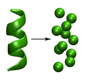
Relative entropy minimized (REM) models of DDA were iteratively parameterized using the Adversarial Residual Coarse-Graining⁵³ software framework (git repository available upon request). Analysis and visualization used the theano⁵⁴, numpy⁵⁵, lightgbm⁵⁶, scikit-learn⁵⁷, shap^{38, 58}, pandas⁵⁹, ggplot2⁶⁰, data.table⁶¹, and pracma⁶² libraries Each iteration’s CG simulation was performed using the settings described above for CG models. Marginal distributions were confirmed to well approximate those implied by the theory underpinning REM (SI). All potentials (bonded and nonbonded) were represented via pairwise interactions. Nonbonded pairwise potentials were represented using a WCA potential summed with a 3rd order $b$-spline (the additive non-spline terms significantly improve stability during training); bonded potentials were represented using a harmonic potential summed with a 3rd order $b$-spline. For nonbonded interactions, 20 equally space spline knots were used for both the bonded and nonbonded splines; the nonbonded splines and tables ranged from 0.001 to 20 Angstroms, and the bonded splines and tables ranged from 0.001 to 10 Angstroms. Both the parameters controlling the WCA and harmonic terms were transformed through $\exp$ to enforce positivity. Bonds were present both between nearest neighbors along the CG backbone and neighbors separated by a single site; in the latter case, the bonded interactions emulated angle potentials. At each iteration, 1.8$e$5 configurations were randomly sampled from atomistic trajectory and used to calculate the REM derivative (along with the entire CG trajectory). Larger sets of configurations for derivatives were not seen to change the REM results, although smaller sets (e.g., 9$e$4) were noted to give biased potentials. For each iterative update, the next set of parameters was generated using the RMSprop algorithm⁶³ using a rate of 0.009 for all parameters (all parameterization was performed relative to LAMMPS real units). Resulting parameter updates were clipped to a absolute maximum of 0.07. Parameters were updated until no reliable change in any potential was visible for 30 iterations.

The radius of gyration and Q-helicity were used to quantify the behavior of DDA; their formulation can be found in Rudzinski and Noid ⁴⁷. Q-helicity quantifies the similarity of a given configuration to a helix: 0 corresponds to no helical character, while 1 corresponds to a completely helical polypeptide. Similar CVs are present in enhanced sampling studies, see Piana and Laio ⁶⁴ and Prakash et al. ⁶⁵.

3.2 Actin

Actin was simulated at the atomistic resolution using GROMACS 5.1.4⁶⁶; the protein was solvated with 29530 waters (TIP3P) and 107 pairs of potassium and chloride ions. Equilibration details may be found in Hocky et al. ⁶⁷. Production simulations were performed for 1 $\mu s$ using CHARMM27+CMAP⁶⁸ in the NPT ensemble at 310$K$ and 1 $bar$ using the stochastic velocity rescaling thermostat⁶⁹ with a coupling parameter of 0.1 $ps$ and a Parrinello-Rahman barostat⁷⁰ with a coupling parameter of 2 $ps$. Hydrogen bonds were constrained via LINCS. Samples were collected every 100 $ps$. The atomistic frames were mapped to the CG resolution using the map found in Saunders and Voth ⁷¹. Briefly, sites indexed 1-4 represent actin’s four main subdomains which are approximately arranged at the 4 corners of a square; site 9 represents the nucleotide ADP situated at the center of these 4 subdomains, and site 5 represents the D-loop, a semistructured region connected to site 2. The map is characterized in Fig. 2 (adapted from Saunders and Voth ⁷¹ with permission). Hetero-elastic network models (hENMs) were created using the procedure in Lyman et al. ⁷² using this atomistic trajectory. In certain portions of the results, models are parameterized using all 12 of these sites. In other portions only sites 1-4 are used.

Figure 2: The map used to coarse-grain actin in the current study. Each set of atoms was mapped to a position via a center of mass mapping. CG models of actin were simulated and modeled at both the resolution of all 12 sites presented and at the resolution of sites 1-4.

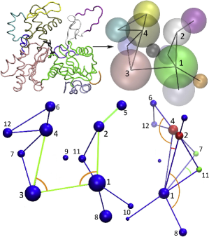
CG samples of actin were generated using LAMMPS (version 17Nov2016). Initial configurations were taken from the mapped atomistic trajectory. The system was propagated using a timestep of 1 $fs$ via a Langevin thermostat with a damping parameter of 50 $fs$. 2$e$5 CG samples were obtained by sampling every 10 $ps$. The relaxation steps used for actin were less aggressive than those used in DDA as no REM optimization was needed. When performing classification based comparisons, similar procedures were followed except the size of the data was significantly smaller: 1$e$4 samples were used from each data source (the entirety of the mapped atomistic simulation was used, and the CG trajectory was randomly subsampled).

4 Results

SHAP coordinates were used to explain errors in models of DDA and actin. As elaborated on in section 3.1, when considering DDA a single resolution of 12 sites was used with multiple pairwise spline force-fields, each of which was minimized using REM. The CG resolution was defined as the center of mass of each amino acid. In the case of actin, models consisting of fully connected networks of harmonic springs at two resolutions (12 and 4 sites) were studied, each of which were parameterized using the hENM method as described in section 3.2; as a result, all harmonic springs present differed. Section 4.1 studies the effect of various force-field bases on DDA, providing examples of using SHAP based analysis to understand and improve existing force-fields. Section 4.2 analyzes the role of the CG map when modeling actin, providing an example of how $\Delta U$ and the resulting SHAP coordinates relate to selecting model resolution.

4.1 Dodecaalanine

Dodecaalanine was modeled using five different force-fields. Each force-field was composed solely of pairwise interactions at the bonded and nonbonded level. Sites adjacent along the backbone were connected via bonds; sites separated by a single site were connected via an additional bond to emulate a angle potential. Within each type of interactions (bonded, angle-bonded, and nonbonded), a unique interaction type was defined for each possible pair of site types. Each model can be considered as extending the model before it.

The first model was composed of a single site type. The pairwise nonbonded interactions were set to be constant, i.e. nonbonded pairwise forces were uniformly zero. This resulted in unique two pairwise interactions (one bonded and one angle bonded). The second model was identical to the first model, but included pairwise nonbonded interactions. The third model then included a single additional collective site type for the termini, resulting in two site types total. The fourth extended the model by considering the site types at each termini to be distinct, resulting in three site types. The final model was extended to five site types by providing additional unique site types to each CG bead adjacent to a termini bead. The difference in the pairwise potentials derived when adding new site types is substantial, as shown in the SI. Only a subset of these models is analyzed in certain sections for brevity.

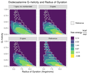
Established CVs, such as the radius of gyration and Q-helicity (see section 3.1), show significant differences between the reference atomistic data and the various models: high helical states are not captured. The difference between a select few models and the reference free energy surface is shown in Fig. 3. However, little difference is apparent between various CG force-fields, save for a small amount of extra distortion present in the single site model lacking nonbonded interactions.

Figure 3: Free energy surfaces of the radius of gyration and Q-helicity for various models and the reference distribution. The grey overlay (and lower right panel) is given by the reference density and is present as a visual guide. Clear differences exist between the models and the reference distribution, but little difference can be seen between various models, despite significant differences in pairwise potentials (see SI).

Classification was performed between each model and the reference data, with the results shown in Fig 4. We note that Fig. 4 characterizes the distribution of errors at the resolution of the CG Hamiltonian, but that $\Delta U$ is also a valid structural CV⁷³ that is optimized to separate the pair of ensembles it is generated from. $\Delta U$ additionally numerically corresponds to the difference in pointwise free energy values at the resolution given by considering $\Delta U$ as a CV. There exist other CVs that equivalently recapitulate $\Delta U$, including the distribution in the full SHAP feature space. The dimensionally reduced coordinates are not guaranteed to share this property, but seem to recapitulate the overlap shown by $\Delta U$ alone.

Figure 4: Violin plots of $\Delta U$ for multiple models of dodecaalanine. Each model distribution is divided along the reference and model ensembles. Note that varying models modify $\Delta U$, changing the shape of the projected reference distribution.

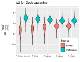
In contrast to the lack of change present in Fig. 3, increasingly complex force-field bases produces notable changes in the distribution of $\Delta U$. More significant drops in the magnitude of error can be seen after addition of nonbonded interactions and the introduction of a third site type. Interpreting $\Delta U$ as a typical CV, it is also apparent that all of the models considered have relatively poor overlap with the reference data set.

4.1.1 Uniform no-nonbonded model

SHAP variables were constructed for the 1 type DDA model lacking nonbonded interactions using the per-feature output of TreeExplainer as input for UMAP based dimensional reduction (Fig. 5).

Figure 5: Free energy surfaces produced along the SHAP CVs generated from the 1 type no-nonbonded model. Light grey lines characterize the combine density of the model and reference data and serve as a visual guide.

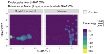
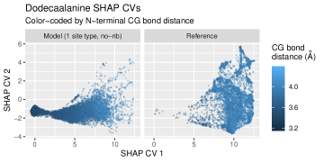
The lack of overlap seen in Fig. 4 is preserved, along with additional organization representing the various sources of error. While UMAP lowers dimensionality to allow visualization, it does not provide explicit formulas for the resulting CVs. However, examination of the individual aggregated SHAP values themselves provides immediate insight into the distances characterizing $\Delta U$. For example, the feature with the largest mean absolute SHAP value by a factor of 3.5 is the N-terminal CG bond; the next set of maximal SHAP values spans distances between sites separate by a single site (e.g. backbone index 3 and backbone index 5). Plotting the N-terminal bond distance with the SHAP CVs (Fig. 6) demonstrates that the elongated error present from $(0,-1.7)$ to $(8,-1.7)$ is primarily due to this bond distance. Larger scale N-terminal effects (combined with minor distortion at the C-terminus) dictate the width of this feature. Comparison of SHAP values via the generated SHAP CVs provides information on their interdependence. For example, comparison of the values of radius of gyration and Q-helicity with the generated SHAP coordinates (SI) implies that the variety of small islands present in the right of the reference ensemble primarily represent both partially helical states and minor bond distance errors in the middle of the protein, while the fully extended configurations are diffusely present around $(8,-1.5)$. While the helical errors are spread across multiple features, they correspond to single islands in the SHAP based projection.

Figure 6: Samples from the 1 type no-nonbonded and reference ensembles projected onto the SHAP CVs in Fig. 5. Samples are colored by the distance between the N-terminal CG site and its nearest bonded neighbor.

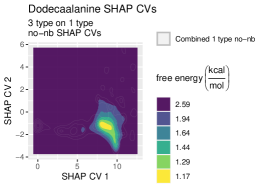
Both non-bonded interactions and a single additional type for the termini (the 2 type model) each reduce the elongated error feature dominating the model lacking nonbonded interactions; however incorporating a distinct bead for each each termini (the 3 type model) fully removes the elongated error present in Fig. 5, as can be seen by projecting the 3 type model ensemble onto the coordinates present in 5 (Fig. 7). The additional site types also slightly increase the density present in various partially helical states, but not sufficiently to register in Fig. 7.

Figure 7: 3 type free energy surface projected along the SHAP CVs generated from the 1 type no-nonbonded model. Filled surfaces represent the 3 type model ensemble, while grey lines represent the combined 1 type no-nonbonded and reference ensembles presented in Fig. 5.

4.1.2 Three-site model

In order to better describe the remaining error in the more complex models, new SHAP CVs were generated based on the comparison of the 3 type ensemble to the reference data (Fig. 8).

Figure 8: The free energy surface projected along the SHAP CVs generated from the 3 site model grey lines characterize the combine density of the model and reference data and serve as a visual guide.

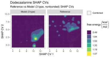
The global geometry described by the resulting SHAP CVs differs significantly from that present in Fig. 5: as expected, the bond errors dominating the 1 type model without nonbonded interactions are no longer present. Inspection of the individual SHAP values no longer isolates a particular portion of the protein as broadly responsible for $\Delta U$ (see SI). The large diffuse area present (as well as the protrusion at $(10,0)$) in the model ensemble is due to erroneous helix-like formation at the C-terminus, a phenomena spread over 4 sites. The subbasins near $(8,2)$, are due to differences in the inner walls present in $\Delta U$. Sharper features around $(4,6.5)$ are due to the remaining helix formation (primarily present though 1-4 distances), while features around $(10,7.5)$ are due to a higher propensity for shorter bond distances and angles throughout the middle of the protein. These types of errors are degenerate along the protein backbone, resulting in many minima in the surface. The complex nature of the presented error makes it difficult to isolate small adjustments to the force-field basis to improve the model. Attempting to improve the quality of the model by adding additional site detail to each termini results in little improvement, consistent with said error analysis. This is seen in both Fig. 4 and 9, where Fig. 9 visualizes the ensemble produced by the 5 type model projected into the coordinates created from the 3 site model.

Figure 9: 5 type free energy surface projected along the SHAP CVs generated from the 3 type model. Filled surfaces represent the 5 type model ensemble, while grey lines represent the combined 3 type and reference ensembles presented in Fig. 8.

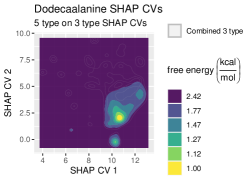
This lack of improvement contrasts strongly the improvement seen in Fig. 7, supporting the view that additional parameters, if not targeted towards known areas of error, do not necessarily improve model performance.

4.2 Actin

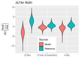
Actin was analyzed using two different elastic network models created using the heteroENM methodology⁷²: one model was created at a 12 site resolution, while the other was created using a 4 site subset of the 12 site model (sites indexed 1 through 4). In order to better understand model error, the samples produced by the 12 site model were additionally mapped to the 4 site resolution for comparison to the 4 site model. The distribution of $\Delta U$ for the 12 site model at both resolutions as well as the errors in the 4 site model are visualized in Fig. 10. At the 12 site resolution, the 12 site model exhibits a large spread of $\Delta U$. When mapped to the 4 site resolution, however, it performs marginally better than the 4 site model when compared to the reference ensemble.

Figure 10: Violin plots of $\Delta U$ for multiple models and resolutions of actin, divided along the reference and model ensembles. The “12 site (4 resolution)” and “4 site” models are compared to the reference at the 4 site resolution, while “12 site” is compared at the 12 site resolution. Note that varying models/resolutions change the form of $\Delta U$, which changes the shape of the projected reference distribution.

SHAP variables were generated between the 12 site elastic network and the reference ensemble (Fig. 11) at the 12 site resolution; a diffuse central basin is present, along with a variety of smaller subbasins. The subbasins present at $(1.5,2.5)$ and $(11,5)$ are due to the distance between sites 1 and 9. The subbasin at $(6,5)$ is attributable to the distance between sites 2 and 4. The subbasin at $(6,-3)$, along with the broadness of the central basin, correspond to relatively uncorrelated heterogeneity occurring between site 5 and the rest of the protein, along with variation in the position of site 9.

Figure 11: The free energy plot given by the SHAP CVs calculated by comparing the 12 site elastic network to the reference ensemble at a 12 site resolution.

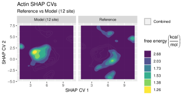
Collectively, the majority of the error present is associated with sites $5$ and $9$, which represent the d-loop (a transiently structured region located on the edge of the protein) and the nucleotide ADP (situated in the center of the protein). This suggests that a model built at the 4 site resolution may result in less error, which is indeed shown in Fig. 10. A harmonic network built at the 4 site resolution was used to test this hypothesis; the resulting SHAP CV based comparison is shown in Fig. 12. Inspection of plotted SHAP values indicates that the horizontal spread (along CV 1) is due to error associated with the 2-4 and 3-4 distances, while the vertical spread is attributable to error in the 1-4 distance.

Figure 12: Free energy surface produced along the SHAP variables generated by comparing a 4 site elastic network model to mapped reference data.

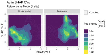
However, $\Delta U$ for the 4 site model is determined at a different resolution than that of the 12 site model. As where the 4 site model is only judged on the behavior of sites 1-4 (which represent the core of each of the 4 main subdomains), the 12 site model is compared using all 12 sites— and as a result must capture more complex behavior. This likely does not align with error validation in practice: if both a 4 site and 12 site model are considered, it is likely that only sites 1-4 are critical (if not, the 4 site model would be an invalid choice regardless of its accuracy). In other words, the pertinent behavior of the 12 site model may very well be concentrated in sites 1-4. The current analysis framework allows us to analyze the 12 site model at the resolution of sites 1-4 by mapping the 12 site model to the 4 site resolution. The resulting mapped 12 site ensemble is then projected onto the variables generated by the SHAP variable 4 site model (Fig. 13).

Figure 13: 12 site free energy surface produced along the SHAP variables generated by comparing a 4 site elastic network model to mapped reference data. Filled surfaces represent the 12 site model ensemble, while grey lines represent the combined 4 site model and reference ensembles presented in Fig. 12.

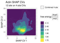
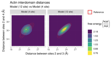
The offset of the 12 site ensemble in CV space (along with Fig. 10) implies that errors related to the 2-4 and 2-3 are resolved in the 12 site model; this is reinforced by considering the free energy surface given by said distances (Fig. 14).

Figure 14: Free energy surface produced the distance between sites 2 and 4 and the distance between sites 2 and 3. Filled contour panels represent the two model ensembles, while the red line contour overlay correspond to statistics from the reference ensemble.

5 Discussion and Conclusions

The results presented demonstrate two uses of SHAP CVs. First, the error of an existing model can be described and used as a guide to adjust the force-field basis. These CVs can similarly be used to quantify the effect of a proposed change to said basis. Second, the effect of resolution on the accuracy of a CG model can be quantified: in this case, an increase in resolution improved the behavior of a CG model quantified at a coarser resolution. While the conclusions and model adjustments are not necessarily counterintuitive, they were analyzed with minimal human intervention.

In the case of DDA, the largest reduction in error was seen when accounting for bond disagreements. This is supported by the fact that the large free energies found in effective bonded interactions can easily result in areas of phase space that are effectively not traversed by either the model or reference data, as a lack of overlap in any dimension implies a lack of overlap at the full phase space resolution. The conclusions drawn from the SHAP CVs contrast strongly with conclusions drawn from pre-selected CVs: while Fig. 3 suggests that the CG model occupies a subset of the phase space favorable to the mapped atomistic data, Fig. 4, along with Figs 5 and 8, illustrate that the two ensembles are close to disjoint, while the latter two figures still represent variation in Q-helicity (and to a lesser extent, radius of gyration). This does not imply that pre-selected CVs cannot correctly discover issues with overlap— $\Delta U$ is a CV in itself and may be selected/approximated using external knowledge.

In the case of actin, it is perhaps surprising that at a 12 site resolution the distribution of $\Delta U$ is of a similar magnitude as that found in DDA: actin has a persistent tertiary structure while DDA is relatively disordered. However, it is important to note that actin was modeled using harmonic potentials as where DDA was modeled using spline interactions. Based on SHAP based analysis, this error is primarily due to difficulty modeling the d-loop and nucleotide, a conclusion supported by the reduction of error when considered at the 4 site resolution. Notably, however, the 12 site model performs better than one constructed without these problematic sites due to improved reproduction of cross correlations. This is attributable to the limited basis of the forcefield, and suggests that approaches which select CG mappings without considering the limited force-field basis that is eventually applied will not produce mapping operators that are necessarily useful in practice. Similarly, if the proposed approach is combined with a series of maps at varying resolutions, the effect of model resolution can be validated in a novel and rigorous way. The interplay between $\Delta U$ and resolution supports the idea that the correctness of an approximate CG model may be difficult to consider without an implied resolution for analysis.

5.1 Invariance and Adversarial Learning

The relationship between $\eta$ and $\Delta U$ (Eq. (2)) provides important insight to classification in the current context. First, if the force-fields generating both ensembles are known, the information provided by classification can alternatively be gleaned by calculating the overall difference in free energies using, for example the Bennet Acceptance Ratio⁷⁴. Similarly, if performing classification between a CG model and a mapped reference ensemble, estimating the ideal classifier is analogous to estimating the true PMF along with the corresponding free energy difference. Additionally, Eq. (2) directly implies that any symmetry or locality shared by $U_{\mathrm{FF}}$ and $U_{\mathrm{PMF}}$ is shared by $\eta$. This has important consequences when considering applying the proposed XAI approach to novel chemical systems: the corresponding classification problem will contain physical symmetries and locality, and approaches which do not take this into account will likely provide poor estimates of $\eta$. A straightforward example is a homogeneous liquid where an asymmetric classifier is trained on the Cartesian coordinates: sampling sufficient to converge various local correlations (e.g., radial distribution functions) may be insufficient to parameterize such a classifier. On the other hand, functions which are formulated to obey permutational and rototranslational symmetries, while widely investigated as techniques for atomistic and CG force-field development^{14, 75, 76}, will require appropriate explanation methods.

Systematic coarse-graining methodologies typically define a numerical measure of error and then return the force-field which minimizes said error. Classification suggests similar ideas of global error based on the accuracy achievable when performing classification between the ensemble implied by the force-field and the reference ensemble: a lower level of mean accuracy implies better emulation of the reference statistics (the accuracy is minimized if the reference and model are indistinguishable; this results in a constant $\eta$ of 0.5). A natural question is then to consider force-fields which are optimized using this particular measure of quality. These force-field optimization approaches lead to adversarial learning, an approach firmly established by generative adversarial networks⁷⁷, which when applied to CG force-field development is termed Adversarial Residual Coarse-Graining (ARCG)⁵³. The properties of $\eta$ described in the previous paragraph additionally often apply to adversarial learning. The error estimation present in ARCG⁵³ can resultingly be viewed as simultaneously providing an estimate of $U_{\mathrm{PMF}}$ and the difference in configurational free energy. Conversely, the variational error in ARCG can be calculated without performing any classification: if a higher order force-field is used to approximate $U_{\mathrm{PMF}}$ and supplemented with a free energy difference method, the derivatives updating the parameters are similarly calculable through (2). Additionally, as $\eta$ is central to adversarial residuals^{36, 53}, the explanations proposed in this article are fundamentally related to global residuals such as relative entropy and the Hellinger distance. The value of these various divergences provide a quantification of the overlap of $\Delta U$ described Figs. 4 and 10; however, the numerical values of these divergences are difficult to interpret without context.

CG models are often created to study specific phenomena, and it may not be necessary to perfectly produce all the behavior of the mapped atomistic system. In this cases the proposed methodology can be adapted by customizing the resolution at which it is performed, such as in the example of actin. However, more broadly, the concept of bottom-up error analysis as presented here may not be appropriate for these models. The modeler must decide whether to view the model as a way to reproduce specific phenomena or whether to view the model as a drop in quantitative replacement for atomistic simulation. Certain coarse-graining strategies, such as ARCG, can parameterize a force-field to reproduce the manybody behavior of a subset of the particles present in the CG system. However, doing so incorporates additional human influence into the creation of said CG model: as the resolution becomes coarser, the approach begins to resemble top-down parameterization strategies. We note that machine learned atomistic force-fields are often quantified including values similar to $\Delta U$; if CG models are to be eventually considered as accurate as their fine-grained counterparts, utilizing similar measures of quality is critical.

5.2 XAI and future directions

The analysis in this article focuses on using SHAP values to describe the behavior produced by CG potentials. The approach trains a classifier to estimate $\Delta U$, and then uses techniques from XAI to explain said estimate. Interpretable models and explanations intrinsically provide a way to understand the high dimensional differences characterizing the quality of a proposed CG force-field, and we fully expect that other methods from the rapidly developing field of XAI will find similar utility. Furthermore, the study of explanations and interpetability is fundamentally relevant to the creation of CG models: CG force-fields are rarely created solely to reproduce the manybody-PMF of the training ensemble. They are instead often created to either extract knowledge from the system under study or to investigate new physical settings, tasks that intrinsically require human understanding of the limitations and workings of the utilized CG model. Any technique for bottom-up CG model creation which uses external human validation is a candidate for using explainable techniques. We hope that this work will serve as an initial example for a new approach to CG model validation.

5.3 References

AEPD thanks Alexander Pak, Glen Hocky, and Sriramvignesh Mani for insight, guidance, and simulation data. This material is based upon the work supported by the National Science Foundation (NSF, Grant No. CHE-1465248). Simulations were performed using the resources provided by the University of Chicago Research Computing Center (RCC).

References

- Karplus and McCammon 2002 Karplus, M.; McCammon, J. A. Molecular dynamics simulations of biomolecules. Nat Struct. Mol. Bio. 2002, 9, 646
- Shaw et al. 2010 Shaw, D. E.; Maragakis, P.; Lindorff-Larsen, K.; Piana, S.; Dror, R. O.; Eastwood, M. P.; Bank, J. A.; Jumper, J. M.; Salmon, J. K.; Shan, Y., et al. Atomic-level characterization of the structural dynamics of proteins. Science 2010, 330, 341–346
- Buch et al. 2010 Buch, I.; Harvey, M. J.; Giorgino, T.; Anderson, D. P.; De Fabritiis, G. High-throughput all-atom molecular dynamics simulations using distributed computing. J. Chem. Inf. Model. 2010, 50, 397–403
- Lindorff-Larsen et al. 2011 Lindorff-Larsen, K.; Piana, S.; Dror, R. O.; Shaw, D. E. How fast-folding proteins fold. Science 2011, 334, 517–520
- Karplus and Lavery 2014 Karplus, M.; Lavery, R. Significance of molecular dynamics simulations for life sciences. Isr. J. Chem. 2014, 54, 1042–1051
- Voth 2008 Voth, G. A. Coarse-graining of condensed phase and biomolecular systems; CRC press, 2008
- Brini et al. 2013 Brini, E.; Algaer, E. A.; Ganguly, P.; Li, C.; Rodríguez-Ropero, F.; van der Vegt, N. F. Systematic coarse-graining methods for soft matter simulations–a review. Soft Matter 2013, 9, 2108–2119
- Saunders and Voth 2013 Saunders, M. G.; Voth, G. A. Coarse-graining methods for computational biology. Ann. Rev. Biophys. 2013, 42, 73–93
- Noid 2013 Noid, W. Perspective: Coarse-grained models for biomolecular systems. J. Chem. Phys. 2013, 139, 09B201_1
- Noid 2013 Noid, W. G. Biomolecular Simulations; Springer, 2013; pp 487–531
- Marrink and Tieleman 2013 Marrink, S. J.; Tieleman, D. P. Perspective on the Martini model. Chem. Soc. Rev. 2013, 42, 6801–6822
- Potestio et al. 2014 Potestio, R.; Peter, C.; Kremer, K. Computer simulations of soft matter: Linking the scales. Entropy 2014, 16, 4199–4245
- Pak and Voth 2018 Pak, A. J.; Voth, G. A. Advances in coarse-grained modeling of macromolecular complexes. Curr. Opin. Struc. Biol. 2018, 52, 119–126
- Gkeka et al. 2020 Gkeka, P.; Stoltz, G.; Barati Farimani, A.; Belkacemi, Z.; Ceriotti, M.; Chodera, J. D.; Dinner, A. R.; Ferguson, A. L.; Maillet, J.-B.; Minoux, H.; Peter, C.; Pietrucci, F.; Silveira, A.; Tkatchenko, A.; Trstanova, Z.; Wiewiora, R.; Lelièvre, T. Machine Learning Force Fields and Coarse-Grained Variables in Molecular Dynamics: Application to Materials and Biological Systems. J. Chem. Theory. Comput. 2020, 16, 4757–4775, PMID: 32559068
- Noé et al. 2020 Noé, F.; Tkatchenko, A.; Müller, K.-R.; Clementi, C. Machine learning for molecular simulation. Annu. Rev. Phys. Chem. 2020, 71, 361–390
- Rudzinski 2019 Rudzinski, J. F. Recent progress towards chemically-specific coarse-grained simulation models with consistent dynamical properties. Computation 2019, 7, 42
- Noid et al. 2007 Noid, W.; Chu, J.-W.; Ayton, G. S.; Voth, G. A. Multiscale coarse-graining and structural correlations: Connections to liquid-state theory. The Journal of Physical Chemistry B 2007, 111, 4116–4127
- Shell 2008 Shell, M. S. The relative entropy is fundamental to multiscale and inverse thermodynamic problems. J. Chem. Phys. 2008, 129, 144108
- Humphrey et al. 1996 Humphrey, W.; Dalke, A.; Schulten, K., et al. VMD: visual molecular dynamics. J. Mol. Graphics 1996, 14, 33–38
- Ceriotti 2019 Ceriotti, M. Unsupervised machine learning in atomistic simulations, between predictions and understanding. J. Chem. Phys. 2019, 150, 150901
- Bartók et al. 2018 Bartók, A. P.; Kermode, J.; Bernstein, N.; Csányi, G. Machine learning a general-purpose interatomic potential for silicon. Phys. Rev. X 2018, 8, 041048
- Stoltz et al. 2010 Stoltz, G.; Rousset, M., et al. Free energy computations: A mathematical perspective; World Scientific, 2010
- Molnar 2020 Molnar, C. Interpretable Machine Learning; Lulu.com, 2020
- Arrieta et al. 2020 Arrieta, A. B.; Díaz-Rodríguez, N.; Del Ser, J.; Bennetot, A.; Tabik, S.; Barbado, A.; García, S.; Gil-López, S.; Molina, D.; Benjamins, R., et al. Explainable Artificial Intelligence (XAI): Concepts, taxonomies, opportunities and challenges toward responsible AI. Inform. Fusion 2020, 58, 82–115
- Arya et al. 2019 Arya, V.; Bellamy, R. K.; Chen, P.-Y.; Dhurandhar, A.; Hind, M.; Hoffman, S. C.; Houde, S.; Liao, Q. V.; Luss, R.; Mojsilović, A., et al. One explanation does not fit all: A toolkit and taxonomy of ai explainability techniques. arXiv preprint arXiv:1909.03012 2019,
- Murdoch et al. 2019 Murdoch, W. J.; Singh, C.; Kumbier, K.; Abbasi-Asl, R.; Yu, B. Definitions, methods, and applications in interpretable machine learning. Proc. Natl. Acad. Sci. U. S. A. 2019, 116, 22071–22080
- Molnar et al. 2020 Molnar, C.; Casalicchio, G.; Bischl, B. Interpretable Machine Learning–A Brief History, State-of-the-Art and Challenges. arXiv preprint arXiv:2010.09337 2020,
- Holzinger et al. 2018 Holzinger, A.; Kieseberg, P.; Weippl, E.; Tjoa, A. M. Current Advances, Trends and Challenges of Machine Learning and Knowledge Extraction: From Machine Learning to Explainable AI. Machine Learning and Knowledge Extraction. Cham, 2018; pp 1–8
- Kodratoff 1994 Kodratoff, Y. The comprehensibility manifesto. 1994; \urlhttps://www.kdnuggets.com/news/94/n9.txt
- Rüping et al. 2006 Rüping, S., et al. Learning interpretable models. 2006,
- Rudin 2019 Rudin, C. Stop explaining black box machine learning models for high stakes decisions and use interpretable models instead. Nat. Mach. Intell. 2019, 1, 206–215
- Mittelstadt et al. 2019 Mittelstadt, B.; Russell, C.; Wachter, S. Explaining explanations in AI. Proceedings of the conference on fairness, accountability, and transparency. 2019; pp 279–288
- Friedman et al. 2001 Friedman, J.; Hastie, T.; Tibshirani, R. The elements of statistical learning; Springer series in statistics New York, 2001; Vol. 1
- Buja et al. 2005 Buja, A.; Stuetzle, W.; Shen, Y. Loss functions for binary class probability estimation and classification: Structure and applications. Working draft, November 2005, 3
- Gneiting and Raftery 2007 Gneiting, T.; Raftery, A. E. Strictly proper scoring rules, prediction, and estimation. Journal of the American statistical Association 2007, 102, 359–378
- Reid and Williamson 2011 Reid, M. D.; Williamson, R. C. Information, divergence and risk for binary experiments. J. Mach. Learn. Res. 2011, 12, 731–817
- Lemke and Peter 2017 Lemke, T.; Peter, C. Neural network based prediction of conformational free energies-a new route towards coarse-grained simulation models. J. Chem. Theory Comput. 2017,
- Lundberg and Lee 2017 Lundberg, S. M.; Lee, S.-I. A unified approach to interpreting model predictions. Adv. Neur. In. 2017; pp 4765–4774
- Lundberg et al. 2020 Lundberg, S. M.; Erion, G.; Chen, H.; DeGrave, A.; Prutkin, J. M.; Nair, B.; Katz, R.; Himmelfarb, J.; Bansal, N.; Lee, S.-I. From local explanations to global understanding with explainable AI for trees. Nat. Mach. Intell. 2020, 2, 2522–5839
- Lundberg et al. 2018 Lundberg, S. M.; Nair, B.; Vavilala, M. S.; Horibe, M.; Eisses, M. J.; Adams, T.; Liston, D. E.; Low, D. K.-W.; Newman, S.-F.; Kim, J., et al. Explainable machine-learning predictions for the prevention of hypoxaemia during surgery. Nat. Biomed. Eng. 2018, 2, 749
- Shapley 1953 Shapley, L. S. A value for n-person games. Contributions to the Theory of Games 1953, 2, 307–317
- Young 1985 Young, H. P. Monotonic solutions of cooperative games. Int. J. Game. Theory 1985, 14, 65–72
- Sundararajan and Najmi 2019 Sundararajan, M.; Najmi, A. The many Shapley values for model explanation. arXiv preprint arXiv:1908.08474 2019,
- Kumar et al. 2020 Kumar, I. E.; Venkatasubramanian, S.; Scheidegger, C.; Friedler, S. Problems with Shapley-value-based explanations as feature importance measures. arXiv preprint arXiv:2002.11097 2020,
- McInnes et al. 2018 McInnes, L.; Healy, J.; Melville, J. Umap: Uniform manifold approximation and projection for dimension reduction. arXiv preprint arXiv:1802.03426 2018,
- Maaten and Hinton 2008 Maaten, L. v. d.; Hinton, G. Visualizing data using t-SNE. J. Mach. Learn. Res. 2008, 9, 2579–2605
- Rudzinski and Noid 2015 Rudzinski, J. F.; Noid, W. G. Bottom-up coarse-graining of peptide ensembles and helix–coil transitions. J. Chem. Theory Comput. 2015, 11, 1278–1291
- Case et al. 2018 Case, D.; Ben-Shalom, I.; Brozell, S.; Cerutti, D.; Cheatham III, T.; Cruzeiro, V.; Darden, T.; Duke, R.; Ghoreishi, D.; Gilson, M., et al. AMBER 2018. University of California, San Francisco 2018,
- Huang et al. 2017 Huang, J.; Rauscher, S.; Nawrocki, G.; Ran, T.; Feig, M.; de Groot, B. L.; Grubmüller, H.; MacKerell, A. D. CHARMM36m: an improved force field for folded and intrinsically disordered proteins. Nat. Methods 2017, 14, 71–73
- Schneider and Stoll 1978 Schneider, T.; Stoll, E. Molecular-dynamics study of a three-dimensional one-component model for distortive phase transitions. Phys. Rev. B 1978, 17, 1302
- Plimpton 1995 Plimpton, S. Fast parallel algorithms for short-range molecular dynamics. J. Comput. Phys. 1995, 117, 1–19
- Shinoda et al. 2004 Shinoda, W.; Shiga, M.; Mikami, M. Rapid estimation of elastic constants by molecular dynamics simulation under constant stress. Phys. Rev. B 2004, 69, 134103
- Durumeric and Voth 2019 Durumeric, A. E.; Voth, G. A. Adversarial-residual-coarse-graining: Applying machine learning theory to systematic molecular coarse-graining. J. Chem. Phys. 2019, 151, 124110
- Theano Development Team 2016 Theano Development Team, Theano: A Python framework for fast computation of mathematical expressions. arXiv e-prints 2016, abs/1605.02688
- Harris et al. 2020 Harris, C. R.; Millman, K. J.; van der Walt, S. J.; Gommers, R.; Virtanen, P.; Cournapeau, D.; Wieser, E.; Taylor, J.; Berg, S.; Smith, N. J.; Kern, R.; Picus, M.; Hoyer, S.; van Kerkwijk, M. H.; Brett, M.; Haldane, A.; del R’ıo, J. F.; Wiebe, M.; Peterson, P.; G’erard-Marchant, P.; Sheppard, K.; Reddy, T.; Weckesser, W.; Abbasi, H.; Gohlke, C.; Oliphant, T. E. Array programming with NumPy. Nature 2020, 585, 357–362
- Ke et al. 2017 Ke, G.; Meng, Q.; Finley, T.; Wang, T.; Chen, W.; Ma, W.; Ye, Q.; Liu, T.-Y. Lightgbm: A highly efficient gradient boosting decision tree. Adv. Neur. In. 2017; pp 3146–3154
- Pedregosa et al. 2011 Pedregosa, F.; Varoquaux, G.; Gramfort, A.; Michel, V.; Thirion, B.; Grisel, O.; Blondel, M.; Prettenhofer, P.; Weiss, R.; Dubourg, V.; Vanderplas, J.; Passos, A.; Cournapeau, D.; Brucher, M.; Perrot, M.; Duchesnay, E. Scikit-learn: Machine Learning in Python. J. Mach. Learn. Res. 2011, 12, 2825–2830
- pandas development team 2020 pandas development team, T. pandas-dev/pandas: Pandas 1.1.3. version v1.1.3, 2020
- Wickham 2016 Wickham, H. ggplot2: Elegant Graphics for Data Analysis; Springer-Verlag New York, 2016
- Dowle and Srinivasan 2019 Dowle, M.; Srinivasan, A. data.table: Extension of ‘data.frame‘. 2019; R package version 1.12.8
- Borchers 2019 Borchers, H. W. pracma: Practical Numerical Math Functions. 2019; R package version 2.2.9
- Hinton et al. 2012 Hinton, G.; Srivastava, N.; Swersky, K. Neural networks for machine learning. Coursera, video lectures 2012, 264
- Piana and Laio 2007 Piana, S.; Laio, A. A bias-exchange approach to protein folding. J. Phys. Chem. B 2007, 111, 4553–4559
- Prakash et al. 2018 Prakash, A.; Baer, M. D.; Mundy, C. J.; Pfaendtner, J. Peptoid backbone flexibilility dictates its interaction with water and surfaces: a molecular dynamics investigation. Biomacromolecules 2018, 19, 1006–1015
- Abraham et al. 2015 Abraham, M. J.; Murtola, T.; Schulz, R.; Páll, S.; Smith, J. C.; Hess, B.; Lindahl, E. GROMACS: High performance molecular simulations through multi-level parallelism from laptops to supercomputers. SoftwareX 2015, 1, 19–25
- Hocky et al. 2016 Hocky, G. M.; Baker, J. L.; Bradley, M. J.; Sinitskiy, A. V.; De La Cruz, E. M.; Voth, G. A. Cations stiffen actin filaments by adhering a key structural element to adjacent subunits. J. Phys. Chem. B 2016, 120, 4558–4567
- Mackerell Jr et al. 2004 Mackerell Jr, A. D.; Feig, M.; Brooks III, C. L. Extending the treatment of backbone energetics in protein force fields: Limitations of gas-phase quantum mechanics in reproducing protein conformational distributions in molecular dynamics simulations. J. Comput. Chem. 2004, 25, 1400–1415
- Bussi et al. 2007 Bussi, G.; Donadio, D.; Parrinello, M. Canonical sampling through velocity rescaling. J. Chem. Phys. 2007, 126, 014101
- Parrinello and Rahman 1981 Parrinello, M.; Rahman, A. Polymorphic transitions in single crystals: A new molecular dynamics method. J. Appl. Phys. 1981, 52, 7182–7190
- Saunders and Voth 2012 Saunders, M. G.; Voth, G. A. Comparison between actin filament models: coarse-graining reveals essential differences. Structure 2012, 20, 641–653
- Lyman et al. 2008 Lyman, E.; Pfaendtner, J.; Voth, G. A. Systematic multiscale parameterization of heterogeneous elastic network models of proteins. Biophys. J. 2008, 95, 4183–4192
- Sultan and Pande 2018 Sultan, M. M.; Pande, V. S. Automated design of collective variables using supervised machine learning. J. Chem. Phys. 2018, 149, 094106
- Bennett 1976 Bennett, C. H. Efficient estimation of free energy differences from Monte Carlo data. J. Comput. Phys. 1976, 22, 245–268
- Goscinski et al. 2020 Goscinski, A.; Fraux, G.; Ceriotti, M. The role of feature space in atomistic learning. arXiv preprint arXiv:2009.02741 2020,
- Anderson et al. 2019 Anderson, B.; Hy, T.-S.; Kondor, R. Cormorant: Covariant Molecular Neural Networks. arXiv preprint arXiv:1906.04015 2019,
- Goodfellow et al. 2014 Goodfellow, I.; Pouget-Abadie, J.; Mirza, M.; Xu, B.; Warde-Farley, D.; Ozair, S.; Courville, A.; Bengio, Y. Generative adversarial nets. Adv. Neur. In. 2014; pp 2672–2680