Galactic Scaling Rules in a Modified Dynamical Model

Abstract

Schulz galactic scaling rules Schulz (2017), which include baryonic Tully-Fisher relation, have been surveyed in this work within the context of a modified dynamical model. These scaling relations are derived by employing the virial theorem and applying equilibrium and stability conditions. The scaling rules are also obtained by dimensional analysis of an integral relation between surface density and circular velocity of disk galaxies. To check the validity of the scaling relations based on observational data, we have defined, based on the properties of the model, the proper equilibrium size $R_{eq}$ and equilibrium velocity $V_{eq}$ of systems. By employing these measures of length and velocity, SPARC data (Lelli et al., 2016a) is used to analyze the results. The viability of the scaling relations is tested and it is shown that, compared to some other measures of length and velocity, $R_{eq}$ and $V_{eq}$ provide the closest fits to the theoretical predictions. We have compared our results with prior works and have concluded that the set of baryonic Tully-Fisher relation plus mass-size relation ( or mass-velocity ) provides an appropriate description of the general characteristics of the systems. Lastly, it is shown that these scaling relations predict a certain evolution of galactic properties with redshift. This behavior provides a chance to examine the cosmic evolution of the present modified dynamical model in future works.

1 Introduction

In considering each particular galaxy, one could observe that different systems display distinct features such as bars, boxes, warps, etc. This approach of close inspection of galactic systems would lead to an intricate classification of galaxies. Using this method, the dynamical behavior of various systems might be understood in detail. However, another productive approach could be the investigation of global properties of galaxies such as luminosity, mass, velocity, size, etc. This second line of research leads to galactic scaling laws. It is reasonable to argue that accurate galactic scaling laws could be used as valuable guidelines toward better understanding the origin and evolution of galaxies. As it is explained by Cappellari (2016), scaling relations provide astronomers with some easily measurable, statistically motivated, characters of galactic systems which are redshift dependent; thus, the results can be compared with the outcome of numerical simulations. Moreover, the evolution of the scaling parameters is indeed expected to depend on various mechanisms of galaxy formation; therefore, the general trend of the evolution could be employed in studying the physics of galaxy formation. However, a dominant challenge in deriving the scaling rules is the issue of the sources of error as it has been discussed by Saintonge and Spekkens (2011) extensively.

One of the most accurate scaling rules is reported by Tully and Fisher (1977) as a relation between luminosity and circular velocity. However, some researchers have provided evidence in support of a baryonic Tully-Fisher relation (BTFR) which correlates the baryonic mass with a characteristic velocity, i.e. the flat velocity, of galactic systems (Freeman, 1999, McGaugh et al., 2000, McGaugh, 2005a, Lelli et al., 2016b). The argument in favour of BTFR is that the scatter in this relation is notably smaller in near-infrared (NIR) compared to ultraviolet or far-infrared. In addition, since NIR luminosity is usually considered as the best measure of the stellar mass, one could conclude that the Tully-Fisher relation primarily describes a link between mass and rotational velocity ($M-V$) (Schulz, 2017). However, it seems that we still have a lot to learn from this scaling relation. For example, Iorio et al. (2017) show that BTFR derived from dwarf irregular galaxies of LITTLE THINGS is in excellent agreement with those of larger scale galaxies; though, Mancera Piña et al. (2019, 2020) report a few isolated gas-rich ultra-diffuse galaxies which deviate clearly from BTFR. See section 6 of Iorio et al. (2017) and Figure 3 of Mancera Piña et al. (2019).

Another scaling rule is proposed by Brandt (1960) as a correlation between mass, velocity and size ( $M-V-R$ ) of galaxies. Also, Schulz (2017) provides four interconnected scaling relations between baryonic mass, radius and velocity of galaxies. These scaling rules are derived based on two simple assumptions - related to the phenomenology of galaxies - and they include BTFR and Brandt (1960) relation. By surveying the literature, one may easily find other works mentioning similar results in various systems (Larson, 1981, Kazanas, 1995).

The origin of galactic scaling rules is considered to be rooted within the governing dynamics of the systems. For example, it is expected in the context of the standard model of cosmology that systematic variation of galactic features with halo properties, i.e. mass, size, etc., could generate galactic scaling relations (White, 1997, Navarro, 2018). In this case, an essential issue is defining a suitable scenario by which one could connect the properties of the dark and baryonic matter to the pure observational characters. Navarro (2018) argues, based on N-body and hydrodynamical simulations, that the self-similar nature of cold dark matter halo is also of critical importance in deriving the scaling rules. In these simulations, the correlations between galaxy’s mass and size with those of halo are found to be highly non-linear. See also Davis et al. (2019) who survey a sample of 48 spiral galaxies and report correlations between maximum disk rotational velocity (and halo’s dark matter ) with spiral arm pitch angle, central velocity dispersion and mass of the central black hole. See Salucci (2019) for a review on the distribution of dark matter in galaxies and its properties.

On the other hand, within theories of modified dynamics and modified gravity one should be able to find the scaling relations based on the modified governing equations. These scaling rules eventually correlate only the observable galactic properties, i.e. no halo is presumed in this viewpoint. See Sanders (2010) for a valuable review on different aspects of the mass discrepancy problem, including the scaling relations.

It is quite interesting that the scaling rules derived by Schulz (2017) show a close connection to MOND (MOdified Newtonian Dynamics) phenomenology because, in deriving these relations, Schulz presumes that the acceleration at the edge of the galactic stellar disk is proportional to the characteristic acceleration of MOND. Proposed by Milgrom (1983a, b, c), MOND considers a modification in Newton’s second law to solve the missing mass problem at galactic scales. The second law of dynamics in this theory is modified to a general form of $\vec{a}\mu(a/a_{0MOND})=\vec{g}$, in which $a$ is the acceleration, $g$ is the gravitational field, $\mu$ is an interpolating function and $a_{0MOND}=1.2\times 10^{-10}m/s^{2}$ is a phenomenological parameter of the model which is close to $cH_{0}$ ( Here, $c$ is the speed of light and $H_{0}$ is the Hubble constant ). See also Famaey and McGaugh (2012) for an excellent review on MOND theory and phenomenology. MOND has had some very interesting predictions such as the externeal field effect (Chae et al., 2020, 2021b, 2021a). Moreover, within the context of MOND, one could infer BTFR from the equation of motion (Milgrom, 1983b) as well as the scale invariance of the theory (Milgrom, 2009). It is important to note that the former method relates the asymptotic speed of the system to its total mass while the latter method connects some measure of the mean squared velocity to the total mass of the object (Milgrom, 2009). The interpretation of MOND phenomenology is still debated; however, this model might be discussed through a Machian viewpoint as a type of vacuum effect (Milgrom, 1999).

In this work, we obtain four scaling rules within the framework of a modified dynamical model ( MOD ) which is derived by imposing Neumann boundary condition on general relativistic field equations (Shenavar, 2016a, Shenavar and Javidan, 2020). The model, which is based on Wheeler’s interpretation of Mach’s principle (Wheeler, 1964), is reviewed in Sec. 2. The scaling rules are established based on two different approaches: In the first approach, reported in Sec. 3, the scaling laws are found as a result of "collective behavior" of the systems by forcing the equilibrium and stability conditions based on virial theorem. The second approach uses the modified Poisson equation to find an integral relation between the baryonic surface density and the circular velocity. Then, the scaling rules are derived based on the dimensional analysis of this integral. See A. These two derivations show that the scaling relations could be obtained from the first principles as well as averaged properties of the of the systems.

To analyze the scaling relations, we have defined measures of mass, velocity and scale length based on characteristics of baryons in each galactic systems. Then, a sample of galactic data known as SPARC (Lelli et al., 2016b, a) is used to check the reliability of the scaling laws. Some implications of these scaling rules are discussed in Discussions 6 and Conclusion 7.

From data analysis point of view, if there are $n$ parameters $\left\{x_{1},...,x_{n}\right\}$ describing a system, then one could check for $2^{n}-n-1$ ( $=$ number of subsets containing more than one element ) relations between them; however, not all of these relations are independent because they involve the same quantities. For example, if we presume that there are only three characteristics of a galactic system - namely mass $M$, velocity $V$ and radius $R$ - then there could be four correlations. These relations could be displayed as $M-V$, $M-R$, $V-R$ and finally $M-V-R$; though, only two of the relations could be considered as independent. Because performing a plane fit when there is a collinearity problem is typically more challenging than the simple line fit ( this issue happens in the case of $M-V-R$ relation, see Sec. 5 ), it is wise to choose the relations containing two parameters. However, the above argument is based on the presumption that the measures of mass, scale, velocity and also the underlying model ( concerning the nature of dark matter / gravity ) are well-understood and verified. This is not the case in galactic systems; thus, we have to be careful in interpreting the results. As we will see in Sec. 4, there are various proposals for characteristic velocity and length of the system. The nature of mass discrepancy at galactic scale too is still debated. Thus, it is more cautious to fit all three bivariate relations. The results will be provided in Sec. 5. Clearly, sharp deviations from theoretical predictions in any of the relations could signal anomalies due to unsuitable measures, false theories or even new parameters ( such as the presence of dark halos ).

2 Properties of the model

2.1 Review on the Modified Dynamical Model

The dominant current view toward gravitation is based on the assumption that the laws of local physics, presented through some differential equations, are independent of the universe at large scales ( which is mainly discussed as boundary conditions ). See Hawking and Ellis (1973), page 1. In other word, it is usually presumed that the interaction of two point masses here does not depend on the existence of matter far away. This work is based on a model which presumes otherwise. In other words, in the present model, a connection between local and global physics is prescribed.

The gravitational interaction is described through Einstein field equations which consist of ten partial differential equations (PDE). In this system of coupled PDEs, four equations are constraint equations ( due to Bianchi identity $\nabla^{\mu}G_{\mu\nu}=0$ ) while the rest govern the fabric of spacetime. See Misner et al. (1973), page 409, for a detailed discussion. Similar to other PDEs, Einstein field equations - even in their linearized form - do not uniquely determine the geometry; i.e. one needs to provide suitable boundary conditions to derive a unique solution. For example, according to Thorne et al. (1973), the usual demand in solving the field equations that the scalar potentials should go to zero at spatial infinity is a type of boundary condition.

The implementation of boundary conditions on GR field equations had been interpreted by Wheeler (1964) as Mach’s principle. The model that we apply here has been derived based on imposing Neumann boundary condition ( BC ) on Einstein field equations (Shenavar, 2016a, Shenavar and Javidan, 2020). Assume the following perturbed flat Friedmann-Lemaitre-Robertson-Walker metric

$$ds^{2}=-(1+2\Phi)dt^{2}+R^{2}(t)(1-2\Psi)\delta_{ij}dx^{i}dx^{j}$$ (1)

in which the parameter $R(t)$ is the scale factor while the scalar potentials $\Phi$ and $\Psi$ are, in general, functions of spacetime coordinates. Using this metric, one could derive the Einstein field equations order by order. For example, it is easy to see that if the anisotropic stress is negligible, then the tidal forces would be equal $\partial_{i}\partial_{j}\Phi=\partial_{i}\partial_{j}\Psi$. This equation relates the two scalar potentials and when the boundary condition is imposed on a sphere with the radius of particle horizon, then it is possible to show that due to the homogeneity and isotropy of the cosmos at large scale, the most general solution would be found as $\Phi-\Psi=c_{1}(t)$. This relation shows that, due to the presence of cosmic matter at large scale, the gravitational potential $\Phi$ and the 3-curvature perturbation $\Psi$ could in general be different. See Shenavar and Javidan (2020) for detailed derivation.

According to the present model, a nonzero Neumann parameter $c_{1}(t)$ indicates the effect of distant stars on local dynamics. In the language of Ellis (2013), this is a type of top-down causation. The boundary, i.e. the sphere defined by the particle horizon, is itself evolving; therefore, the Neumann parameter $c_{1}(t)$ evolves with time and this evolution could be determined from the system of equations presented in Appendix A of Shenavar and Javidan (2020). However, according to these equations, the parameter $c_{1}(t)$ changes very slowly in recent cosmic times. Thus, when one is considering the physics of the local universe, as we will do here, one could simply assume this parameter as a constant $c_{1}(t)=c_{1}$. The value of $c_{1}$ should be estimated from observations (Shenavar, 2016a, b, Shenavar and Ghafourian, 2018). It could be shown that for a system of particles, with the density $\rho(\vec{x}^{~{}\prime})$ and total mass $M$, one could derive the next modified potential (Shenavar, 2016b)

$$\Phi(\vec{x})=-G\int\frac{\rho(\vec{x}^{~{}\prime})d^{3}\vec{x}^{~{}\prime}}{|\vec{x}^{~{}\prime}-\vec{x}|}+\frac{2c_{1}a_{0}}{M}\int\rho(\vec{x}^{~{}\prime})d^{3}\vec{x}^{~{}\prime}|\vec{x}^{~{}\prime}-\vec{x}|.$$ (2)

in which $G$ is the gravitational constant and $a_{0}\equiv cH_{0}$ is a fundamental acceleration of the model related to the expansion of the Universe. Thus, the first term on the right hand side ( RHS ) is the Newtonian potential while the second one is due to the new boundary condition. Using this potential, it is possible to obtain the motion of objects in solar system and galactic scales. Based on observations at these scales, one could see that the values $a_{0}\equiv cH_{0}=6.59\times 10^{-10}~{}m/s^{2}$ and $c_{1}=0.065$ are compatible with the data (Shenavar, 2016b, Shenavar and Ghafourian, 2018). At the scale of the solar system, for example, the second term on the RHS of Eq. 2 suggests a small, though detectable, correction to the precession of perihelion of the objects (Shenavar, 2016b). It should be mentioned that such effect occurs as a result of coupling between the zero and the first order terms in an expanding universe. In other words, such term could not appear in a static universe because adding a constant of integration to the scalar potential would not change the force in the static universe.

Theories with a new linear potential, i.e. a constant acceleration or a Rindler term, have been proposed before to address the mass discrepancy problem. For example, we could mention fourth order conformal gravity (Mannheim and Kazanas, 1989, 1994, Mannheim, 2006), five-dimensional brane world unification of space, time and velocity (Carmeli, 2003, Behar and Carmeli, 1999) and Grumiller’s effective theory of gravity (Grumiller, 2010, 2011). Also, many works in the literature have followed this line of thought to fit the basic parameters of the modified models (O’Brien and Mannheim, 2012, Mannheim and O’Brien, 2012, Lin et al., 2013).

Regarding Eq. 2, we point out that having a new potential term, which is proportional to the distance of the two particles $i$ and $j$, i.e. $\propto|\vec{x}_{i}-\vec{x}_{j}|$, the long range interaction in the present model is significantly enhanced compared to the pure Newtonian one ( in which the potential behaves as $\propto 1/|\vec{x}_{i}-\vec{x}_{j}|$ ). This would provide a critical clue in following analysis when we introduce a scale length for gravitating systems.

In the history of potential theory, a potential similar to our modified dynamical term, i.e. $\int\rho(\vec{x}^{~{}\prime})d^{3}\vec{x}^{~{}\prime}|\vec{x}^{~{}\prime}-\vec{x}|$, has been named "superpotential" by Chandrasekhar and Lebovitz (1962a, b, c). These authors surveyed the properties of this term to investigate the stability of astrophysical objects, such as Jacobi ellipsoids, by employing higher ranks of tensor virial theorem. See also Roberts (1962).

From Eq. 2 it is convenient to derive the modified Poisson equation as

$$\nabla^{2}\Phi=4\pi G\rho+\frac{4c_{1}a_{0}}{M}\int\frac{\rho(\vec{x}^{~{}\prime})d^{3}\vec{x}^{~{}\prime}}{|\vec{x}^{~{}\prime}-\vec{x}|}$$ (3)

while, since $\nabla^{2}\int\rho(\vec{x}^{~{}\prime})d^{3}\vec{x}^{~{}\prime}|\vec{x}^{~{}\prime}-\vec{x}|=-2\int\frac{\rho(\vec{x}^{~{}\prime})d^{3}\vec{x}^{~{}\prime}}{|\vec{x}^{~{}\prime}-\vec{x}|}$, one could obtain the next fourth-order Poisson equation (Shenavar and Ghafourian, 2018)

$$\nabla^{4}\Phi=4\pi G\nabla^{2}\rho-\frac{16c_{1}\pi a_{0}}{M}\rho.$$ (4)

In most occasions, this fourth-order differential equation provides a more convenient starting point for the simple reason that it is a pure differential equation while Eq. 3 is an integro-differential equation. However, as we will see in the following, Eq. 3 could also provide a good insight into the physical behavior of the model specially when we are trying to compare the results of the present model with those of the dark matter models. See Sec. 2.2 below.

The left hand side ( LHS ) of Eq. 4 appears mostly in the theory of linear elasticity and it is known as the biharmonic equation. Any solution of Laplace equation is also a solution to the biharmonic equation; though, the opposite is not correct. See Chapter 8 of Selvadurai (2013) for a review on this equation, its properties and solutions. Also, for an investigation on the existence and uniqueness of the solutions of the biharmonic equation see Bhattacharyya and Gopalsamy (1988).

The potential 2 predicts that at outer parts of galaxies which the Newtonian term dies-off, the modified term provides a constant acceleration as $2c_{1}a_{0}$ ( neglecting the long range interaction with the environment ). This prediction has been tested by using a sample of 101 high surface brightness ( HSB ) and low surface brightness ( LSB ) galaxies (Shenavar, 2016a). The value of $c_{1}=0.065$ was found to be in accordance with those derived based on rotation curve data ( a sample of 39 LSB galaxies tested in Shenavar (2016b) ) and perihelion precession. See also Figure A2 in Shenavar and Javidan (2020) which is based on 551 objects and shows similar results.

The general behavior of the rotation curve of a galaxy with central surface density $\Sigma_{0}$ in the present model is dependent to the ratio of $\mathcal{R}_{F}\equiv\Sigma_{\dagger}/\Sigma_{0}$ which one could call the Freeman ratio (Shenavar and Ghafourian, 2018). Here, $\Sigma_{\dagger}=a_{0}/G=9.9~{}kgm^{-2}$ is a critical surface density. The value of $\Sigma_{\dagger}$, when interpreted as a surface brightness, is close to the one found by Freeman (1970) who first suggested that there is a universal surface brightness for spiral galaxies (Famaey and McGaugh, 2012). As discussed in Shenavar (2016b) in more details, galaxies with low mass densities, i.e. when $\Sigma_{0}$ is small compared to $\Sigma_{\dagger}$, show a clear rising rotation curve, those galaxies with intermediate to high-mass surface densities display flat rotation curves while galaxies with the highest masses show a Keplerian decline in their rotation curves. From observational point of view, this behaviour has been reported, for example, by Casertano and van Gorkom (1991).

The local stability of stellar and fluid disks in this modified dynamical model has also been investigated and it has been shown that systems governed by Eq. 4 are locally more stable compared to the Newtonian model (Shenavar and Ghafourian, 2018). Moreover, it could be seen, using WKB approximation, that LSB galaxies are more stable than HSBs; thus, the central surface density of galaxies is critical in understanding the local stability. The role of the central surface density will be discussed more in following.

At cosmic scales, we should point out that choosing Neumann BC to solve cosmic perturbation equations would also change the trajectory of massless particles which results in a new lensing equation (Shenavar, 2016a, Shenavar and Javidan, 2020). The lensing equation of MOD has been tested against a sample of ten strong lensing systems (Shenavar, 2016a). While the derived mass of nine systems are found to be within the observational bound, one lens, i.e. Q0142-100, shows a 7.5 $\%$ deviation from the lower mass bound which is acceptable regarding uncertainties in the position of the image and specially the oblateness of the lens (Shenavar, 2016a). The growth of the cosmic structures too, was studied by a Newtonian approach for which the model predicted a more rapid rate of the structure formation in matter dominated era. Moreover, it is proved that this modified dynamical model displays a late time accelerated expansion with an equation of state which converges to $w<-1$ (Shenavar and Javidan, 2020). Balakrishna Subramani et al. (2019) provide a comparison between the present model and $\Lambda CDM$ ( $\Lambda~{}+$ cold dark matter ) based on angular size - redshift data.

Although Eq. 2 has been derived by modifying the first principles, i.e. the boundary condition of GR plus including the measurement process of spacetime intervals (Shenavar, 2016a, Shenavar and Javidan, 2020), it represents eventually a modified dynamical model. In fact, the behavior of the present model at galactic scales shows some similarities with MOND because both models are constructed based on presuming a universal scale of acceleration. However, it should be pointed out that different proposed interpolating functions of MOND have all resulted in nonlinear models (Famaey and McGaugh, 2012) while Eq. 2 is clearly linear. This feature makes analytical computations much easier as we will see in following. The linearity of the governing equation of motion could also lead to more straightforward galactic simulations. This is the subject of a future work.

2.2 Comparing $\rho_{c_{1}}$ and various dark matter profiles

A definitive solution to the problem of mass discrepancy, whether it is found to be dark matter or modified models of dynamics/gravity, has to explain the apparent successes of the rival models. For example, if models of dark matter are finally approved, they should be able to explain why the universal acceleration of MOND, and its interpolating function, are valuable in explaining galactic systematic. On the other hand, a good modified model of gravity should illustrate the reason that some dark matter profiles are more consistent with the rotation curve data. Here, we will explain a connection between hypothetical dark matter profiles and the extra term in the modified Poisson equation 3.

Figure 1: Comparing the prediction of $\rho_{c_{1}}$ ( solid curve ) for the missing mass with various dark matter density profiles of the Galaxy. Properties of different halos are derived from Weber and de Boer (2010). The CDM profiles are as follows: NFW (Navarro et al., 1996, 1997), BE (Binney and Evans, 2001), Moore (Moore et al., 1999) and pseudo-isothermal ( PISO ). In addition, we have plotted a halo profile named as 240 which is similar to the pseudo-isothermal model of CDM, though, it declines faster at outer parts of the galaxy compared to PISO (Weber and de Boer, 2010).

It is clear that the modified Poisson equation 3 could be rewritten as $\nabla^{2}\Phi=4\pi G(\rho_{m}+\rho_{c_{1}})$ in which

$$\rho_{c_{1}} = \frac{c_{1}a_{0}}{\pi GM}\int\frac{\rho_{m}(\vec{x}^{~{}\prime})d^{3}\vec{x}^{~{}\prime}}{|\vec{x}^{~{}\prime}-\vec{x}|}$$ (5)

plays the role of dark matter halo, i.e. it provides the system with more attractive force. In Fig. 1, we have plotted various density profiles of CDM, for our Milky Way Galaxy, to make a comparison with $\rho_{c_{1}}$. The CDM profiles used here are Navarro, Frenk $\&$ White ( NFW ) (Navarro et al., 1996, 1997), Binney $\&$ Evans ( BE ) (Binney and Evans, 2001), Moore (Moore et al., 1999) and pseudo-isothermal ( PISO ). Also, the halo profile named as 240 is similar to the pseudo-isothermal model of CDM, though, it decreases faster at outer parts of the galaxy (Weber and de Boer, 2010). The free parameters of these halos for the Milky Way Galaxy are provided in Table. 1 of Weber and de Boer (2010). The appropriate density and scale of the baryonic matter are also derived from Weber and de Boer (2010). As it is shown in Fig. 1, in very small radii the prediction of $\rho_{c_{1}}$ for the missing mass density is very close to the profile 240 of Weber and de Boer (2010); then, it converges mostly to BE profile for $0.1~{}(kpc)~{}<R<~{}8~{}(kpc)$. The density $\rho_{c_{1}}$ surely does not diverge at the center as some dark matter profiles do. See, for example, the behavior of NFW at $R\approx 0$ in Fig. 1. At large radii, $\rho_{c_{1}}$ shows a larger value compared to other profiles. This means a larger centripetal force compared to other dark matter halos at large radii. Of course, this results is obtained based on the assumption that the source of gravity is isolated. However, most galaxies are within their group; thus, in general, one expects non-negligible external forces. The external forces might have some effects on galactic scaling rules as we will discuss below.

2.3 Baryonic surface density and the dynamical acceleration

Assume the second-order modified Poisson equation of 3. Since $\nabla^{2}\Phi=-\vec{\nabla}.\vec{a}$, one could estimate to the lowest order the magnitude of change in the gravitational acceleration due to an extended object by $|\nabla^{2}\Phi|\approx|\vec{a}|/L$, in which $L$ is the typical size of the system. In addition, one may write $\rho\propto M/L^{3}$ and $\int\frac{\rho(\vec{x}^{~{}\prime})d^{3}\vec{x}^{~{}\prime}}{|\vec{x}^{~{}\prime}-\vec{x}|}\propto M/L$. Thus, one would expect a relation between the magnitude of the centripetal acceleration, and the baryonic surface density $\Sigma_{b}\propto M/L^{2}$ of the form of

$$a=A_{MOD}\Sigma_{b}+B_{MOD}$$ (6)

in which $A_{MOD}$ and $B_{MOD}$ are some constants which should be determined from observations. Of course, other modified models of gravity are expected to display somehow similar relations at galactic scale, because, these models too are solely dependent to baryonic mass distribution and their scale length. In the case of MOND, for example, we expect a relation as $a=A_{MOND}\Sigma^{1/2}_{b}$ ( see (Famaey and McGaugh, 2012) ) while for pure Newtonian theory, without dark matter halo, one could obtain a relation as $a=A_{Newt}\Sigma_{b}$. The Poisson equation within the dark matter models, on the other hand, provides a relation between baryonic and halo mass and their appropriate scales. Therefore, a simple relation between the acceleration and the baryonic surface density is not expected through dark matter paradigm unless one could prove that there is a fine-tuned relation between baryonic and dark masses and disk-halo sizes. To check the relation between the baryonic surface density and acceleration we will use data from Famaey and McGaugh (2012) who provide the acceleration at the peak of the rotation curve $a_{p}$ and the characteristic surface density of the baryons.

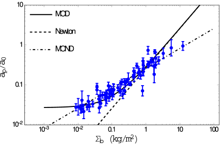
Figure 2: Typical acceleration of galaxies ( in units of $a_{0}=6.59\times 10^{-10}~{}m/s^{2}$ ) as a function of baryonic mass surface density $\Sigma_{b}~{}$ ( in units of $~{}kg/m^{2}$ ). The acceleration $a_{p}$ is measured at the distance where the rotation velocity of baryons is maximum. Data is derived from Famaey and McGaugh (2012). See also Fig. 7 of Lelli et al. (2017) for a similar graph which includes many individual measurements across galaxy rotation curves rather than using peak velocity for each object.

In Fig. 2, we have plotted the data with theoretical curves of MOD, MOND and Newtonian models. The curves correspond to $A_{MOD}/a_{0}=0.26m^{2}/kg$ and $B_{MOD}/a_{0}=0.027$ for MOD model while $A_{MOND}/a_{0}=0.26m/kg^{0.5}$ and $A_{Newt}/a_{0}=0.26m^{2}/kg$ for MOND and Newtonian models, respectively. In this plot, we have assumed $a_{0}=6.59\times 10^{-10}~{}m/s^{2}$ as mentioned above. As one could see from Fig. 2, the curves corresponding to MOND and MOD are more consistent with the data. Although, in Fig. 2 there appears a noticeable deviation between the data and MOD at the very high surface densities, i.e. the last three data points on the right. However, even at this limit, the MOD curve is touched by the error bars of the two data points while the last data point displays a significant deviation from the model. At low surface densities, on the other hand, the MOD curve follows the data pretty well while MOND does the same two. The pure Newtonian line shows a significant discrepancy, especially for systems with lower surface densities. This is of course expected because the Newtonian model is not supposed to justify the galactic systematics without a dark matter halo. From this perspective, Fig. 2 could be thought as an illustration for the mass discrepancy problem in Newtonian model. Also, it is seen from Fig. 2 that the predictions of MOND and MOD are quite different for galaxies with very high and very low surface densities. Especially, the MOD model predicts a constant acceleration ( at redshifts near zero ) for galaxies with very small densities while MOND predicts a decreasing acceleration as $a\propto\Sigma^{1/2}_{b}$. Thus, systems with very low surface densities could help to compare these two models of modified dynamics.

Another important feature of MOND and MOD is that both these models predict an upper bound on $\Sigma$ (Milgrom, 1989, Shenavar and Ghafourian, 2018). In fact, McGaugh (1996) provides detailed analysis on disk galaxies and shows that the number of HSB galaxies with surface densities larger than $\Sigma_{\dagger}\equiv a_{0}/G$ decreases exponentially. This is while HSB galaxies could be observed more easily because they have higher surface brightness compared to LSBs. See, also, Fig. 6 in Shenavar and Ghafourian (2018). In Fig. 2, and for the objects with very high surface densities, there is a clear deviation between MOND and MOD which could help us to compare the two models. More data on this tail of the plot could be helpful to decide between the two modified models of dynamics.

A similar graph to Fig. 2 could be seen in Fig. 7 of Lelli et al. (2017) , which is plotted based on many individual measurements of rotation curves. These authors investigate the link between baryons and dark matter in 240 galaxies and report that the observed acceleration correlates ( over 4 dex ) with the expectations from baryonic distribution. The relations is known as Radial Acceleration Relation (RAR) and it indicates a systematic deviation from Newtonian gravity below the critical acceleration of $\sim 10^{-10}m/s^{2}$. See also McGaugh et al. (2016).

It is important to note that the discussion presented in this section is based on dimensional analysis; thus, Fig. 2 essentially displays an estimated relation between a characteristic acceleration, i.e. $a_{p}$, and the baryonic surface density. For more accurate investigations, one should refer to accurate data analysis of galactic rotation curves or try to find more accurate "scaling rules", as presented in the next sections.

3 Galactic Scaling Rules Derived From the Virial Theorem

In this section, we will derive four scaling relations based on the virial theorem. The validity of these scaling relations would be tested against SPARC data (Lelli et al., 2016a) in the following two sections by introducing characteristic measures of velocity and size for galactic systems.

Here, we will use the steady state plus stability conditions to derive the scaling rules of galactic systems. If a system is in steady state, then its moment of inertia, i.e. $I$, is a constant. Using the scalar virial theorem,

$$\frac{1}{2}\frac{d^{2}I}{dt^{2}}=2T+W,$$ (7)

in which $T\equiv 1/2\int\rho d^{3}\vec{x}~{}\vec{v}^{2}$ and $W\equiv-\int\rho d^{3}\vec{x}~{}(\vec{x}.\vec{\nabla}\Phi)$ stand for the total kinetic energy and the virial energy respectively, one could write the steady state condition as

$$2T+W=0.$$ (8)

See Collins (1978) and also chapters 4 and 7 of Binney and Tremaine (2008) for more details.

Geometry	$\alpha$	$\beta$
Homogeneous sphere	3/5	18/35
Exponential sphere	5/32	7/4
Exponential disk (thin)	$11.63/(4\pi^{2})$	1.47
Exponential disk (thick)	0.28	1.48

Table 1: The virial parameters $\alpha$ and $\beta$. The virial parameters for the first three geometries are derived by Shenavar (2016b). By the same method, one could derive the virial parameters for a thick exponential disk, i.e. the last case.

For a single-component gravitating system, and by using our modified dynamics, it has been previously proved that the virial energy is of the general form of

$$W(R)=-\alpha\frac{GM^{2}}{R}-2c_{1}\beta Ma_{0}R$$ (9)

in which $\alpha$ and $\beta$ are some positive parameters solely dependent to the mass distribution of the system (Shenavar, 2016b). See Table 1 for typical values of $\alpha$ and $\beta$. The virial parameters $\alpha$ and $\beta$ for the first three geometries are derived in Appendix of (Shenavar, 2016b). For the last case, i.e. thick exponential disk, the parameters $\alpha$ and $\beta$ are derived numerically by assuming that the vertical mass distribution of the disk changes as $sech(z/z_{0})/(\pi z_{0})$ in which $z_{0}$ is the scale height of the system presumed to be $1/10$ of the disk radius. In fact, one could show that by assuming the vertical mass distribution as $sech^{2}(z/z_{0})/(2z_{0})$, the results for $\alpha$ and $\beta$ would be almost the same. Thus, $\alpha=0.28$ and $\beta=1.48$ appropriately represent the virial parameters of a thick exponential disk.

In addition to the steady state condition, i.e. Eq. 8, one needs a stability criterion to explain the behavior of the gravitating systems. Here, we maximize the virial energy to find the stable state. The idea of maximizing virial energy to find the scaling relation of galactic systems is first exploited by Secco. See, for example, Secco (2000, 2001). From physical point of view, Eq. 8 suggests that when the virial energy is maximum, the kinetic energy should be minimum. See Fig. 3 which displays the virial energy of a thin exponential disk ( with the scale length $R_{d}$ ) as a function of $y=R/(2R_{d})$ for different values of Freeman ratio $\mathcal{R}_{F}\equiv\Sigma_{\dagger}/\Sigma_{0}=0.1,~{}1.0,~{}10$. We have chosen the thin exponential disk for the sake of convenience; however, it could be easily checked that the general behavior of $W(R)$ in Eq. 9 is similar for other mass distributions.

Figure 3: The virial energy of a thin exponential disk ( in units of $Ma_{0}R_{d}$ ) as a function of $y=R/(2R_{d})$ and for different values of Freeman ratio $\mathcal{R}_{F}=0.1,~{}1.0,~{}10$. To plot this graph, we have assumed $\alpha=11.63/(4\pi^{2})$ and $\beta=1.47$. It is easy to see that every system possesses a maximum of virial energy which corresponds to a minimum of kinetic energy. In addition, for systems with smaller Freeman ratio ( denser galaxies ), the maximum occurs in larger radii ( compared to $R_{d}$ ).

It is clear from Fig. 3 that for systems with smaller Freeman ratio, i.e. denser systems, the maximum of the virial function occurs in larger radii. In fact, it could be proved that for any thin exponential disk one has $y_{max}\propto\mathcal{R}^{-1/2}_{F}$ in which $y_{max}$ is the radius for which the maximum of $W(R)$ happens. Thus, the maximum point of denser systems occurs in larger radii ( in units of $2R_{d}$ ). Moreover, the maximum point of systems with smaller Freeman ratio occurs in smaller virial energies, i.e. larger values of $|W(R)|$. Thus, from Eq. 8, one could immediately realize that because in the steady state condition we have $T=-1/2W$, the dense systems possess larger kinetic energies, i.e. greater velocities for denser galaxies. This behavior has been reported before based on the observations of galaxies (Casertano and van Gorkom, 1991).

Now, we obtain the four scaling rules by assuming an stable equilibrium for galactic systems. The derivation is quite general because we only presume the virial theorem 8 and the general form of the virial energy 9. Hence, no specific mass distribution is assumed. To do so, we note that for a general system with the virial energy of 9, and by maximizing $W(R)$ function, one could find the radius in which the system is in stable virial equilibrium as

$$R_{eq}=\sqrt{\frac{GM\alpha}{2c_{1}a_{0}\beta}}.$$ (10)

This is one of the scaling rules. This relation is reminiscent of the definition of the MOND transition radius for a point mass. It is easy to see that, except for the constants of the model like $a_{0}$ and $\beta$ etc., this expression for the equilibrium radius is only related to the mass of the system.

Now, using the steady state condition 8 and the stability condition 10 one could find a relation between the total mass of the system and its characteristic velocity in virial equilibrium $V_{eq}$ as

$$V^{4}_{eq}=8c_{1}a_{0}\alpha\beta GM$$ (11)

To derive this relation, we replace $T=1/2MV^{2}_{eq}$ and $W|_{R_{eq}}$ from Eq. 9 into Eq. 8. This is the second scaling relation (BTFR).

The scale length of the system could also be found by eliminating mass $M$ from Eqs. 10 and 11 as

$$R_{eq}=\frac{V^{2}_{eq}}{4\beta c_{1}a_{0}}.$$ (12)

which, except for the constants of the model, is only dependent to the virial velocity $V_{eq}$ of the system. Equation 12 is the third scaling relation. It is also possible to derive this scale length directly from the steady state condition of 8

$$-\alpha\frac{GM^{2}}{R_{eq}}-2c_{1}\beta Ma_{0}R_{eq}+MV^{2}_{eq}=0$$

where, by solving for $R_{eq}$ results in

$$R_{eq}=\frac{V^{2}_{eq}\pm\sqrt{V^{4}_{eq}-8c_{1}a_{0}\alpha\beta GM}}{4\beta c_{1}a_{0}}.$$

Using Eq. 11 we see that in the last equation we have $V^{4}_{eq}-8c_{1}a_{0}\alpha\beta GM=0$ and therefore we obtain Eq. 12 again.

Finally, combining any pair of these three scaling relations, i.e. 10, 11 and 12, one can find another scaling law between mass, velocity and scale length as:

$$V^{2}_{eq}R_{eq}=2\alpha GM.$$ (13)

These four scaling rules are closely interconnected because they have been derived from simultaneous imposition of stability and equilibrium conditions in the context of modified dynamics 2. However, only two of the relations could be considered as independent as discussed in the Introduction. Being derived from the virial theorem, these scaling relations characterize the whole system and in particular they do not hold at a certain radial distance.

The interconnectivity of these four scaling rules is displayed in Fig. 4. As Schulz (2017) has explained, versions of these relations have been well known in the literature (Brandt, 1960, Larson, 1981, Kazanas, 1995); though, in some prior works, researchers have used magnitude rather than baryonic mass to discuss the relations. Schulz derives all of these scaling rules by an elegant line of reasoning based on two propositions. The first assumption is that the centripetal acceleration at the edge of the galaxy is proportional to the predicted acceleration of Newtonian physics. Second, this acceleration is a constant which is related to MOND constant acceleration $a_{0MOND}$. However, it should be mentioned that there is another constant in Schulz’s proposal which is named as flatness factor or $C_{f}$. This constant is defined as the "increased gravitational force due to a flattened mass distribution versus a point mass" (Schulz, 2017). The constant $C_{f}$ helps to fit the data to the scaling rules; though, it only changes the intercepts in $\log-\log$ planes. See our discussion on data analysis below for a similar situation.

Figure 4: The Four scaling relations which are derived from virial theorem plus assuming a new modified dynamics governed by potential 2. The parameters $\alpha$ and $\beta$ are dimensionless factors of order unity which are reported in Table. 1 for different geometries.

While Eq. 13 appears usually in researches related to the dark matter paradigm (it is also the oldest of the four rules (Brandt, 1960) ), some scaling relations similar to Eqs. 10, 11 and 12 have attracted much attention in MOND literature. In fact, by noticing that the typical centripetal acceleration at the edge of galactic systems is almost constant, i.e. $V^{2}/R\approx a_{0}$, Milgrom (1983a) started the whole MOND model. This observation is similar to Eq. 12. Moreover, Milgrom explained the mass-velocity scaling rule, i.e. $M\propto V^{4}$, which was first reported by Tully and Fisher (1977) as a relation between luminosity and circular velocity.

In addition to the above method, it is also possible to obtain the four scaling relations of Fig. 4 by dimensional analysis of the modified Poisson equation. We have reported such derivation in A. In comparison, however, the virial method manifests its advantage over the method of dimensional analysis because by using the former method one could introduce measures of virial size and velocity of the systems ( and their uncertainties ). Then, it is possible to employ these measures to investigate the reliability of the scaling rules using relatively accurate data. In what follows, we introduce measures of galactic mass, size and velocity for the SPARC sample, and subsequently, we will study the slopes and intercepts of the scaling relations.

4 Measures of Galactic Mass, Size and Velocity in Virial Equilibrium

In this section, we will define proper measures of mass, size and velocity of galactic systems based on data provided by SPARC (Lelli et al., 2016a). It should be mentioned that these three parameters are introduced in a way that they represent the whole system ( stellar + gas ).

4.1 SPARC data

The SPARC (Spitzer Photometry and Accurate Rotation Curves) galactic sample, provided by Lelli et al. (2016a), includes 175 nearby objects with high-quality data for rotation velocity derived based on HI/H$\alpha$ studies. SPARC also uses new surface photometry at $3.6~{}\mu m$ which traces the stellar mass. Lelli et al. (2016b) employ SPARC data to study the BTFR. To do so, they provide an algorithm to exclude galaxies with rising rotation velocity $V_{f}$, some systems with very high inclination corrections and also objects with low-quality rotation curves. This leaves the sample with 118 galaxies.

Four objects ( out of 118 ) do not possess the scale length of the stellar disk $R_{d}$ and/or $R_{HI}$. The quantity $R_{HI}$ is the radius where the $HI$ surface density, corrected to face-on, reaches $1~{}M_{\odot}/pc$. These two scales are needed ( as we will see below ) to define a suitable virial size for galaxies. Thus, these systems, i.e. NGC 5907, D 631-7, NGC 5533 and NGC 7339, will be excluded from our analysis. Therefore, our sub-sample includes 114 objects. This sub-sample of SPARC is suitable for our data analysis because it covers a wide range of galactic morphology ( S0 to Im ), galactic radius $(~{}0.3~{}kpc\lesssim R\lesssim 15~{}kpc~{})$, gas fraction $f_{g}=M_{g}/M_{b}$ of the systems $(~{}0.01\lesssim f_{g}\lesssim 0.95~{})$, galactic baryonic mass $(~{}10^{8}M_{\odot}\lesssim M_{b}\lesssim 10^{11}M_{\odot}~{})$ and surface brightness of the systems $(~{}8~{}L_{\odot}/pc^{2}\lesssim\Sigma\lesssim 3000~{}L_{\odot}/pc^{2}~{})$. In addition, merging systems have been excluded from the main sample. This point makes the data even more appropriate since our arguments are essentially based on virial theorem which becomes significantly more complicated in the case of merging systems. Beside this, merging systems display out-of-equilibrium HI kinematics which artificially increase the final scatter in the results. In conclusion, the sample which is used here represents non-merging objects in environments with small densities.

4.2 The measure of mass

Virial method dictates the use of total baryonic mass instead of luminosity, and in our following data analysis, we will employ this measure of mass to carry out the calculations. In fact, McGaugh et al. (2000) have shown that the optical Tully-Fisher relation breaks down for velocities less than $100~{}km/s$ while by considering the total baryonic mass, the relation is tight over five decades of stellar mass and circular velocities ranging over $30~{}km/s\lesssim V\lesssim 300~{}km/s$. As Lelli et al. (2016b) have explained ( Sec. 2.3 ) the total baryonic mass in SPARC is derived from $M_{b}=M_{g}+\Upsilon_{\star}L_{[3.6]}$ in which $M_{g}=1.33M_{HI}$ is the mass of gass, 1.33 being included to contain the share of helium, $\Upsilon_{\star}$ is the mass-to-light ratio of stars assumed to be $0.5$ throughout and finally $L_{[3.6]}$ is the $[3.6]$ luminosity. The uncertainty in $M_{g}$ is reported to be generally smaller than $10~{}\%$ which will be used to estimate $\delta f_{g}/f_{g}$ in Eq. 18 below. The collected uncertainty in the total baryonic mass $M_{b}$ due to errors in $M_{g}$, $L_{[3.6]}$, $\Upsilon_{\star}$ and distance has been carefully calculated by Lelli et al. (2016b). Moreover, the error in flat velocity $V_{f}$ due to non-rotational velocities, asymmetries between the two sides of the disk, the dispersion around average velocity and the inclination correction is also provided in SPARC.

4.3 Equilibrium radius of real systems

To fit the above scaling relations, one needs to introduce an appropriate dynamical length scale for real galactic systems. This length scale must represent the two components of the systems, i.e. stellar and gas ( hereafter shown by indices $s$ and $g$ respectively ), and their collective gravitational effects. However, this is not a trivial work due to some observational and theoretical reasons. From observational point of view, the issue is that one can define many scale lengths for the stellar component such as the effective radius $R_{eff}$, which encompasses half of the total luminosity, and also $R_{d}$ which provides the scale length of the stellar disk. The scales $R_{eff}$ and $R_{d}$ are provided in SPARC catalog. On the other hand, for the gaseous component, SPARC provides $R_{HI}$ as defined above. None of these scale length are necessarily compatible with the statistical nature of the virial theorem; however, these are the best available options provided by SPARC. There are other characteristic radii such as $R_{200}$, which is defined as the length where the average density is $200$ times larger than the critical density of the universe. We do not consider this scale length here.

From theoretical point of view, the main issue is to find a dynamical scale length, i.e. a combination of $R_{d}$ ( or $R_{eff}$ ) and $R_{HI}$, to represent the virial size of the systems. To do so, it is necessary to derive a radius based on virial energy of compound ( gas + stars ) systems. We have provided the detailed calculations of the virial energy of a system consisting of gas and stars in B. To first order of approximation, the virial energy of such system is

$$-W_{tot} \simeq G\left[\alpha(\frac{M^{2}_{g}}{R_{g}}+\frac{M^{2}_{s}}{R_{s}})+\gamma_{1}\frac{M_{s}M_{g}}{R_{g}}\right]+\frac{2c_{1}a_{0}}{M}\left[\beta(M^{2}_{g}R_{g}+M^{2}_{s}R_{s})+\gamma_{2}M_{s}M_{g}R_{g}\right]$$ (14)

in which $\gamma_{1}$ and $\gamma_{2}$ are some dimensionless parameters related to the gravitational interaction of gaseous and stellar components. Also, $M_{s}$ $(~{}M_{g}~{})$ and $R_{s}$ $(~{}R_{g}~{})$ are the mass and scale length of the stellar ( gaseous ) system respectively while $M$ is the total mass of the system. In the above formula, we have presumed that stellar and gas systems have the same geometry; thus, they both have the same virial coefficients $\alpha$ and $\beta$. This simplification reduces the number of degrees of freedom in our data analysis.

Now, to find the equilibrium radius, imagine that there is a system with total mass $M$, radius $R$ and the virial energy of

$$-W=\alpha^{\prime}\frac{GM^{2}}{R}+2c_{1}\beta^{\prime}Ma_{0}R$$

which is equivalent to the virial energy of of the original system, i.e. $W=W_{tot}$. By equating the last two formulas for virial energy, one could find a quadratic equation for $R$ with two solutions. We define the arithmetic mean of the two roots as the equilibrium radius:

$$R_{eq}=\frac{GM}{4c_{1}a_{0}\beta^{\prime}}\left[\alpha(\frac{f^{2}_{g}}{R_{g}}+\frac{(1-f_{g})^{2}}{R_{s}})+\gamma_{1}\frac{f_{g}(1-f_{g})}{R_{g}}\right]+\frac{1}{2\beta^{\prime}}\left[\beta(f^{2}_{g}R_{g}+(1-f_{g})^{2}R_{s})+\gamma_{2}f_{g}(1-f_{g})R_{g}\right]$$ (15)

in which $f_{g}=M_{g}/M$ is the ratio of the mass of the gas to the total baryonic mass. There are six dimensionless parameters, i.e. $c_{1}$, $\alpha$, $\beta$, $\beta^{\prime}$, $\gamma_{1}$ and $\gamma_{2}$, in the definition of $R_{eq}$ which only four of them could be independent. Thus, we redefine these parameters as $\lambda_{1}=\alpha/(4\beta^{\prime}c_{1})$, $\lambda_{2}=\gamma_{1}/(4\beta^{\prime}c_{1})$, $\lambda_{3}=\beta/(2\beta^{\prime})$, $\lambda_{4}=\gamma_{2}/(2\beta^{\prime})$ to simplify the expression for $R_{eq}$ as

$$R_{eq}=\frac{GM}{a_{0}}\left[\lambda_{1}(\frac{f^{2}_{g}}{R_{g}}+\frac{(1-f_{g})^{2}}{R_{s}})+\lambda_{2}\frac{f_{g}(1-f_{g})}{R_{g}}\right]+\lambda_{3}(f^{2}_{g}R_{g}+(1-f_{g})^{2}R_{s})+\lambda_{4}f_{g}(1-f_{g})R_{g}$$ (16)

Also, in our data analysis below, we have used the value $\Sigma_{\dagger}=a_{0}/G=4.7\times 10^{9}M_{\odot}/kpc^{2}$ for the critical surface density.

To see the behavior of the equilibrium radius as a function of Freeman ratio $\mathcal{R}_{F}=\Sigma_{\dagger}/\Sigma_{0}$, we have plotted $R_{eq}$ in Fig. 5 for the objects of SPARC sample. Here, $\Sigma_{0}=M/\pi R^{2}_{eq}$ is assumed as the proper surface density of the system with the scale length $R_{eq}$. Also, the plot is drawn by assuming $R_{s}=R_{eff}$ and $(~{}\lambda_{2},~{}\lambda_{3},~{}\lambda_{4}~{})/\lambda_{1}=(~{}1.1,~{}0.039,~{}0.19~{})$ which are the best parameters derived from the data analysis in Sec. 5. A similar graph could be produced if one assumes $R_{s}=R_{d}$ in deriving $R_{eq}$. See also Fig. 11 which shows the change in $R_{HI}$, $R_{eff}$ and $R_{d}$ as a function of Freeman ratio. By comparing Figs. 5 and 11, it could be seen that the behavior of $R_{eq}$ as a function of $\mathcal{R}_{F}$ is more similar to $R_{HI}$ than $R_{eff}$ or $R_{d}$.

Eq. 16 means that when $\mathcal{R}_{F}$ is small, the equilibrium radius is determined by the first term on the RHS of this equation, i.e. the term proportional to $GM/a_{0}$. In other words, when $\mathcal{R}_{F}$ is small, the system is dominated by the Newtonian gravitational energy. On the other hand, when $\mathcal{R}_{F}$ is large, the terms proportional to $\lambda_{3}$ and $\lambda_{4}$ in Eq. 16 have a dominant share in the equilibrium radius. These terms are due to MOD virial energy. In conclusion, $R_{eq}$ puts galaxies with large and small Freeman ratios on the same plane; thus, the scatter in size-dependent relations ( $M-R$ and $V-R$ ) decreases significantly.

Another advantage of using $R_{eq}$ as a scale length of galactic systems ( instead of $R_{d}$ or $R_{eff}$ ) is that $R_{eq}$ includes the stellar and gaseous sizes with their appropriate share in the systems ( $1-f_{g}$ and $f_{g}$ respectively). This is particularly important because in some systems, the gas contributes more mass than the stars ( up to 95 $\%$ in a few objects of SPARC ). Of course, using $R_{d}$ or $R_{eff}$ as the representative of the scale of the system would not be fitting in such situation anymore.

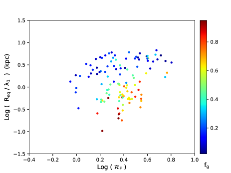
Figure 5: Equilibrium radius $R_{eq}$ as a function of Freeman ratio $\mathcal{R}_{F}$. In this plot it is assumed that $R_{s}=R_{eff}$ and $(~{}\lambda_{2},~{}\lambda_{3},~{}\lambda_{4}~{})/\lambda_{1}=(~{}1.1,~{}0.039,~{}0.19~{})$. It could be seen that the gas-rich systems ( galaxies with high $f_{g}=M_{g}/M_{b}$ ) are separated from gas-poor ones. A similar graph could be achieved if one assumes $R_{s}=R_{d}$ in deriving $R_{eq}$. See also Fig. 11 which shows the change in $R_{HI}$, $R_{eff}$ and $R_{d}$ as a function of Freeman ratio. Color online.

It could be seen in Fig. 5 that the gas-rich systems are separated from gas-poor ones. Moreover, very few objects could be found with $\mathcal{R}_{F}<1$. This is due to the reason that in MOD dynamics, systems with $\Sigma_{0}\gtrsim\Sigma_{\dagger}$ are locally unstable. See Shenavar and Ghafourian (2018) for the detailed proof.

The equilibrium radius $R_{eq}$ depends on four observable parameters $R_{s}$, $R_{g}$, $M$ and $f_{g}$. The error in this radius could be estimated as

$$\delta R_{eq}=\left((\frac{\partial R_{eq}}{\partial R_{s}}\delta R_{s})^{2}+(\frac{\partial R_{eq}}{\partial R_{g}}\delta R_{g})^{2}+(\frac{\partial R_{eq}}{\partial M}\delta M)^{2}+(\frac{\partial R_{eq}}{\partial f_{g}}\delta f_{g})^{2}\right)^{1/2}$$ (17)

in which

$$\frac{\delta f_{g}}{f_{g}}=\sqrt{\left(\frac{\delta M_{g}}{M_{g}}\right)^{2}+\left(\frac{\delta M}{M}\right)^{2}}$$ (18)

represents the error in gas fraction. All necessary quantities to calculate $\delta R_{eq}$ are provided by SPARC.

4.4 Equilibrium Velocity

The kinetic energy in virial theorem 7 contains both rotational and random terms. In the same way, the equilibrium velocity $V_{eq}$, which represents a system in virial equilibrium, must contain both rotation and pressure tracers. A suitable velocity which fulfills this condition could be introduced as

$$V_{eq}=\left(0.5V^{2}_{f}+\sigma^{2}_{eq}\right)^{1/2}$$ (19)

where $\sigma_{eq}$ is the velocity dispersion, i.e. it is a measure of disordered or noncircular motions. Some authors (Weiner et al., 2006, Kassin et al., 2007, Cortese et al., 2014) have proposed a similar measure of velocity to include the share of the gas velocity dispersion. However, here $\sigma_{eq}$ represents the velocity dispersion in both gas and stars.

Fitting Parameters				$\log R_{eq}=a+b(\log M_{b}-\log M_{b0})$				$\log R_{eq}=a+b(\log V_{eq}-\log V_{eq0})$				$\log M_{b}=a+b(\log V_{eq}-\log V_{eq0})$
$\frac{\lambda_{2}}{\lambda_{1}}$	$\frac{\lambda_{3}}{\lambda_{1}}$	$\frac{\lambda_{4}}{\lambda_{1}}$	$\frac{\sigma_{eq}}{(km/s)}$	$a$	$b$	$\Delta$	$\epsilon_{y}$	$a$	$b$	$\Delta$	$\epsilon_{y}$	$a$	$b$	$\Delta$	$\epsilon_{y}$
0.80	0.046	0.21	14	0.178	0.483	0.080	0.0	0.178	1.865	0.13	0.0	10.136	3.91	0.21	0.082
0.95	0.043	0.17	13	0.127	0.497	0.083	0.0	0.134	1.937	0.13	0.0	10.137	3.889	0.21	0.082
1.10	0.039	0.19	15	0.146	0.498	0.082	0.0	0.15	1.937	0.13	0.0	10.134	3.932	0.21	0.083	$\surd$
1.10	0.036	0.18	10	0.136	0.503	0.071	0.0	0.137	1.933	0.13	0.0	10.142	3.834	0.21	0.081
1.30	0.037	0.18	14	0.140	0.502	0.071	0.0	0.138	1.957	0.13	0.0	10.136	3.910	0.21	0.082
1.45	0.037	0.19	17	0.148	0.490	0.083	0.0	0.149	1.963	0.13	0.0	10.130	3.981	0.21	0.085
1.55	0.035	0.21	11	0.169	0.487	0.083	0.0	0.163	1.870	0.13	0.0	10.141	3.851	0.21	0.081

Table 2: Results from fitting the bivariate scaling relations of Fig. 4. It is assumed that the size of the stellar disk is equal to $R_{eff}$. Data from SPARC (Lelli et al., 2016b, a). The plots corresponding to the set of parameters indicated by $\surd$ are provided in Figs 6, 7 and 8.

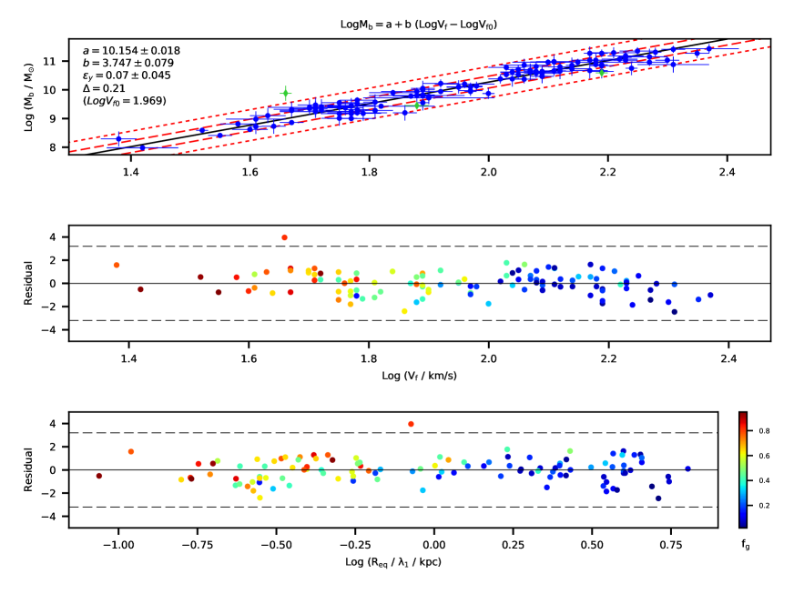
Figure 13: A decreased slope is observed for BTFR $M\propto V^{4}_{eq}$ presuming that $\sigma_{eq}=0$, i.e. in this graph $V_{eq}=V_{f}$. The equilibrium radius $R_{eq}$ in lower residual plot is calculated by assuming $R_{s}=R_{eff}$ and $(\lambda_{2},~{}\lambda_{3},~{}\lambda_{4})/\lambda_{1}=(1.1,~{}0.039,~{}0.19)$. Also, compare with Fig. 8. Data from SPARC (Lelli et al., 2016b, a). Color online.

It could be easily seen that although the correction due to $\sigma_{eq}$ is negligible for most galaxies with $V_{f}\gtrsim 40$, the overall effect of this term is considerable. To see this point, consider BTFR. In this relation, the correction of $\sigma_{eq}$ shifts the objects with smallest $V_{f}$ toward right on velocity axis while it keeps data points with high velocities almost unchanged. Thus, the slope in BTFR increases from $\simeq 3.7$ to $\simeq 3.9$ and higher. Compare Figs 8 and 13 to see this point. Adding $\sigma_{eq}$, which we assume to be smaller than $20~{}km/s$ in our data analysis, could help us to find unified scaling rules for pressure-dominated and rotation-dominated galaxies; though, this matter needs a much larger sample and is beyond the scope of our work.

The error in $V_{eq}$ could be simply estimated because the error in $V_{f}$ is provided by SPARC. We should mention that Lelli et al. (2019) have reported a minor indexing bug in the calculations of the error in $V_{f}$ provided by Lelli et al. (2016b). However, this bug causes an underestimation of the errors by $0.6~{}km~{}s^{-1}$ on average which corresponds to $0.1~{}\%$ deviation in the final results; thus, we neglect it here.

5 Data Analysis

5.1 Method of data analysis

From statistical analysis point of view, and due to large uncertainties in most galactic data, the data analysis of galactic scaling rules is a challenging issue. The related least-square problem has been discussed in many works (Akritas and Bershady, 1996, Tremaine et al., 2002, Press et al., 2007). Here, we use the method which has been explained in Sec. 3.2 of Cappellari et al. (2013) to perform robust line fit to data with uncertainties in all parameters and also possible unknown intrinsic scatter. This method combines the Least Trimmed Squares (LTS) robust procedure which is suggested by Rousseeuw (1984) for the first time and then improved by Rousseeuw and Van Driessen (2006). This technique also forces the fit to converge to the appropriate solution in the presence of significant outlier data points (Leroy and Rousseeuw, 1987). The outlier data are shown by green diamonds in all fitting plots below. Cappellari’s code automatically excludes the outliers from the fit.

For a thorough review on the method which is used here, one could refer to Cappellari et al. (2013). To fit a linear relation of the form $y=a+b(x-x_{0})$ between two data sets $x_{i}$ and $y_{i}$, with error bars on both axes $\delta x_{i}$ and $\delta y_{i}$, and also intrinsic scatter in the y-coordinate $\epsilon_{y}$, one can minimize the quantity

$$\chi^{2}=\sum^{N}_{i}\frac{\left(a+b(x_{i}-x_{0})-y_{i}\right)^{2}}{(b\delta x_{i})^{2}+\delta y^{2}_{i}+\epsilon^{2}_{y}}$$ (20)

in which N is the number of data points, to find the best fit. The value of the intrinsic scatter is found iteratively by forcing the fit toward the point that $\chi^{2}$ per degrees of freedom , i.e. $\chi^{2}/(N-2)$, converges to unity. In other words, in this method the chi-by-eye rule is always satisfied by enforcing it on the fit.

In each of the following fits, the observed root-mean-square ( rms ) scatter $\Delta$ in dex would be provided in the graph. In addition, the plot for Studentized residual is provided in every case. Also, in the residual plots we have used Grubbs’s critical value, as a simple measure, to indicate the possible outliers (Grubbs, 1969).

The scaling relation $M\propto V^{2}R$ could be analyzed by a plane fit method which is also provided by Cappellari et al. (2013). In this case, however, there appears the issue of collinearity of $V$ and $R$ parameters because, as we will see below, these two parameters are strongly correlated. In the case of perfect collinearity, one could not find a unique solution to the regression problem because the matrix involved is not invertible. Non-exact, but still significant, correlations between independent variables could still produce inaccurate results. See Feigelson and Babu (2012), page 198, for a discussion on this matter. Although a variety of procedures have been suggested to deal with such situations, we do not consider them here because the issue is beyond the scope of our work. Thus, $M-V-R$ relation would not be fitted in our data analysis. The data analysis presented here examines the scaling rules derived based on MOD; thus, this analysis is model dependent.

5.2 Results

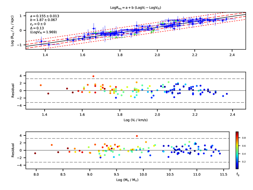
Figure 12: Data analysis of the scaling rule $R_{eq}\propto V^{2}_{eq}$ presuming that $\sigma_{eq}=0$, i.e. in this graph $V_{eq}=V_{f}$. The equilibrium radius $R_{eq}$ is calculated by assuming $R_{s}=R_{eff}$ and $(\lambda_{2},~{}\lambda_{3},~{}\lambda_{4})/\lambda_{1}=(1.1,~{}0.039,~{}0.19)$. It is seen that the slope is decreased compared to the cases with $\sigma_{eq}\neq 0$. Also, compare with Fig. 7. Data from SPARC (Lelli et al., 2016b, a). Color online.

The results of the data analysis are provided in Tables 2 to 4, Figs. 6 to 8 and also Figs. 12 to 17. Because we have five free parameters in $R_{eq}$ and $V_{eq}$, i.e. $\lambda_{1}$ to $\lambda_{4}$ and $\sigma_{eq}$, it is quite hard to probe all of the possible values for these parameters. However, the order of the magnitude of $\lambda_{i}$ could be speculated by using the values of $c_{1}$, $\alpha$, $\beta$, $\gamma_{1}$ and $\gamma_{2}$. Thus, one could restrict the domain of possible values of the parameters. Moreover, we can temporarily decrease the degrees of freedom by dividing $R_{eq}$ by any of $\lambda_{i}$ parameters since we only work with logarithmic values. We choose the parameter $R_{eq}/\lambda_{1}$ which is equivalent to putting $\lambda_{1}=1$. We determine the value of $\lambda_{1}$ at the end of the data analysis by using the zero-points of the scaling rules.

Fitting Parameters				$\log R_{eq}=a+b(\log M_{b}-\log M_{b0})$				$\log R_{eq}=a+b(\log V_{eq}-\log V_{eq0})$				$\log M_{b}=a+b(\log V_{eq}-\log V_{eq0})$
$\frac{\lambda_{2}}{\lambda_{1}}$	$\frac{\lambda_{3}}{\lambda_{1}}$	$\frac{\lambda_{4}}{\lambda_{1}}$	$\frac{\sigma_{eq}}{(km/s)}$	$a$	$b$	$\Delta$	$\epsilon_{y}$	$a$	$b$	$\Delta$	$\epsilon_{y}$	$a$	$b$	$\Delta$	$\epsilon_{y}$
0.80	0.055	0.24	17	0.244	0.496	0.075	0.0	0.237	1.917	0.13	0.0	10.130	3.981	0.21	0.085
0.85	0.056	0.21	18	0.215	0.498	0.076	0.0	0.211	1.970	0.12	0.0	10.128	4.007	0.21	0.085
1.00	0.055	0.21	13	0.215	0.499	0.076	0.0	0.215	1.925	0.12	0.0	10.137	3.889	0.21	0.082
1.10	0.057	0.22	16	0.240	0.491	0.073	0.0	0.225	1.933	0.12	0.0	10.132	3.956	0.21	0.084
1.15	0.058	0.21	17	0.221	0.495	0.076	0.0	0.217	1.951	0.12	0.0	10.130	3.981	0.21	0.085

Table 3: Results from fitting the bivariate scaling relations of Fig. 4 when the size of the stellar disk is assumed as $R_{s}=R_{d}$. Data from SPARC (Lelli et al., 2016b, a).

		$\log R_{eq}=a+b(\log M_{b}-\log M_{b0})$				$\log R_{eq}=a+b(\log V_{f}-\log V_{f0})$
Scale	$\frac{\sigma_{eq}}{(km/s)}$	$a$	$b$	$\Delta$	$\epsilon_{y}$	$a$	$b$	$\Delta$	$\epsilon_{y}$
$R_{eff}$	15	0.526	0.267	0.18	0.102	0.539	1.014	0.21	0.134
$R_{d}$	15	0.394	0.335	0.15	0.0	0.426	1.067	0.16	0.0
$R_{HI}$	15	1.214	0.351	0.11	0.0	1.216	1.554	0.16	0.0

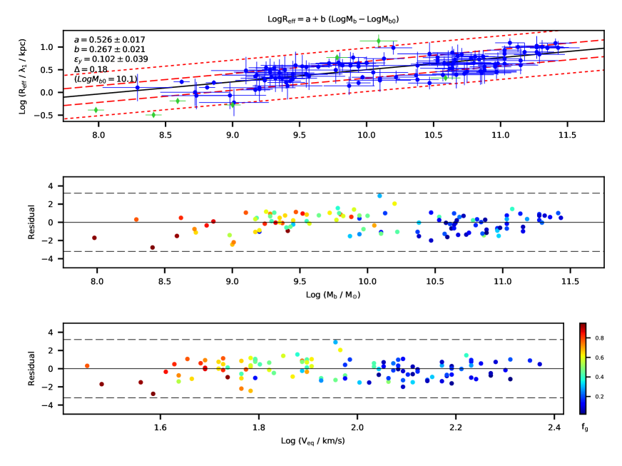
Figure 14: Data analysis of the scaling rule $R_{eff}-M$, i.e. when the scale length of the system is $R_{eff}$ instead of $R_{eq}$, and $\sigma_{eq}=15~{}km/s$. Compare with Fig. 6. Data from SPARC (Lelli et al., 2016b, a). Color online.

Table 4: Fitting the scaling relations for different scale length $R_{eff}$, $R_{d}$, $R_{HI}$ while the velocity dispersion in not negligible ($\sigma_{eq}=15~{}km/s$). Related graphs are shown in Figs. 14 to 19. Data from SPARC (Lelli et al., 2016b, a).

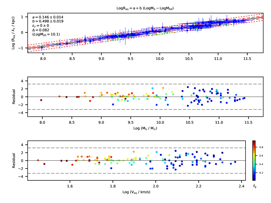
Figure 6: Data analysis of the scaling rule $R_{eq}\propto M^{0.5}$ based on the data of SPARC (Lelli et al., 2016b, a). In this graph it is assumed that $R_{s}=R_{eff}$ and $(~{}\lambda_{2}~{},\lambda_{3}~{},\lambda_{4}~{})/~{}\lambda_{1}=(~{}1.1~{},0.039~{},0.19~{})$ while $\sigma_{eq}=15~{}km/s$. The red dashed ( red dotted ) lines in the upper plot show the $1\sigma$ ( $2.6\sigma$) bands which encloses $60\%$ ( $99\%$ ) of the values assuming a Gaussian distribution (Cappellari et al., 2013). The outlier points, which are automatically excluded from the line fit, are displayed as green diamonds. Studentized residuals are provided in two bottom plots with Grubbs’s critical line ( dashed lines ) as an indicator of outliers. Compare this figure with Figs. 14, 16 and 18 which assume $R_{eff}$, $R_{d}$ and $R_{HI}$ as the scale length of systems ( instead of $R_{eq}$ ) respectively. The objects are color coded by gas fraction $f_{g}=M_{g}/M_{b}$. Color online.

Another point is that the LTS-LINEFIT code forces the fit to a point where $\chi^{2}/(N-2)=1$ as mentioned before; thus, one could not find a single set of best parameters based on minimizing $\chi^{2}$. Instead, we judge the outcomes of the code based on their residual behavior. Many residual plots show linear trend or curvature; these results will be neglected. We systematically search for any pattern ( linear or second order ) in residuals and exclude them. Tables 2 and 3 report the acceptable fitting parameters while the best outcome is distinguished by a $\surd$ sign in Table 2. Table 2 presumes $R_{s}=R_{eff}$ in deriving the equilibrium radius $R_{eq}$ while Table 3 assumes $R_{s}=R_{d}$.

The plots corresponding to the best outcome of the fit, i.e. $(\lambda_{2},~{}\lambda_{3},~{}\lambda_{4})/\lambda_{1}=(1.1,~{}0.039,~{}0.19)$ and $\sigma_{eq}=15km/s$ while $R_{s}=R_{eff}$, are provided in Figs. 6 to 8. For each plot we will report Pearson’s and Spearman’s coefficients as measures of linear relationship and monotonicity of the relationship between two variables respectively (Press et al., 2007). Despite relatively large uncertainties in the data, specially the high error in characteristic radius, one could see that the results are close to the theoretical predictions. Because of the logarithmic scales, the horizontal and vertical axes seem compressed; however, this help us to better present the results of the fit.

Fig. 6 represents the mass-size scaling rule $R_{eq}\propto M^{0.5}_{m}$. The theoretical prediction of the slope lies within the derived bound, i.e. $b=0.498\pm 0.019$. In addition, Pearson and Spearman correlations could be found as 0.98 and 0.97 respectively. Moreover, in this case the intrinsic scatter is negligible while $\Delta=0.082$ dex ($21~{}\%$). Remembering that the baryonic mass is in units of $M_{\odot}$, we could see from the intercept of this relation that

$$\frac{1}{2}\log\left(\frac{G\alpha\lambda^{2}_{1}/(2c_{1}a_{0}\beta)}{kpc^{2}/M_{\odot}}\right)=-4.88\pm 0.21$$ (21)

which will be used below to estimate the parameters $\alpha$, $\beta$, $\lambda_{1}$ and $c_{1}$.

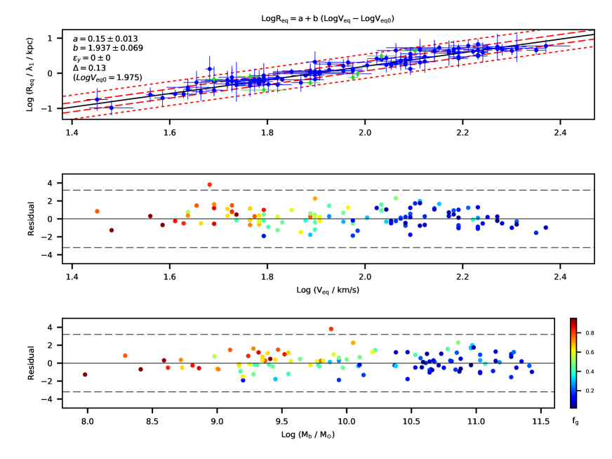
Figure 7: Data analysis of the scaling rule $R_{eq}\propto V^{2}_{eq}$. See Fig. 6 for the related parameters and explanations. Compare with Fig. 12 in which we have assumed $\sigma_{eq}=0$. Also, compare this figure with Figs. 15, 17 and 19 which assume $R_{eff}$, $R_{d}$ and $R_{HI}$ as the scale length of systems ( instead of $R_{eq}$ ) respectively. Color online.

The next scaling rule, i.e. $R_{eq}\propto V^{2}_{f}$, is plotted in Fig. 7. The slope of the plot is $b=1.937\pm 0.069$ while the theoretical prediction is $b=2$. Thus, the derived value contains the theoretical prediction. Also, we mention that in this case the intrinsic scatter is negligible and $\Delta=0.13$ dex. Furthermore, Pearson’s and Spearman’s correlations are derived to be 0.94 and 0.93 respectively. The intercept of the relation is also interesting. Regarding the units which are used in plot 7, i.e. $V_{eq}$ in units of $km/s$ and $R_{eq}$ in units of $kpc$, we could see that an estimation for the fundamental value of $\beta c_{1}a_{0}$ could be derived as

$$\log\left(\frac{4\beta c_{1}a_{0}/\lambda_{1}}{(km/s)^{2}/kpc}\right)=3.68\pm 0.15.$$ (22)

The last scaling rule is the baryonic Tully-Fisher relation which is shown in Fig. 8. The slope is derived as $b=3.932\pm 0.085$ and it includes the theoretical slope of $b=4$. In addition, we have $\Delta=0.21$ dex in this case. Furthermore, BTFR shows Pearson and Spearman correlations as 0.96 and 0.95 respectively. The intercept of the plot is also found as

$$-\log\left(\frac{8c_{1}\alpha\beta a_{0}G}{(km/s)^{4}/M_{\odot}}\right)=-2.37\pm 0.19$$ (23)

which lacks the presence of $\lambda_{1}$ naturally because this scaling rule is not dependent to the size.

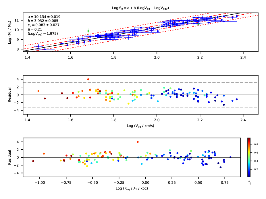
Figure 8: Data analysis of the scaling rule $M\propto V^{4}_{eq}$. See Fig. 6 for the related parameters and explanations. Compare with Fig. 13 in which we have assumed $\sigma_{eq}=0$. Color online.

Conformal and Grumiller gravities, which both display linear potentials similar to MOD, are also shown to be consistent with Tully-Fisher relation (O’Brien et al., 2018, Ghosh et al., 2021). The Tully-Fisher relation, and especially its baryonic version, has been much discussed in the literature. The work by Lelli et al. (2016b), in particular, is important because of their employed sample and method of data analysis. The same code and ( almost ) the same sample is applied here. However, Lelli et al. (2016b) fit the BTFR by weighting each galaxy as $f^{2}_{g}$. By using this assumption, they derive a slope as $b=3.95\pm 0.34$ and a zero point equal to $1.86\pm 0.60$. These authors have also reported the error-weighted fit, i.e. the same method that is used here, by which they have derived $b=3.71\pm 0.08$ and the intercept of $2.27\pm 0.18$. See Fig. 13 for a similar result. Although, the derived slope of BTFR in Fig. 8 is larger because we have used equilibrium velocity $V_{eq}$ in that graph instead of $V_{f}$. As a result, galaxies with smallest velocities move toward right on the velocity axis causing an increase in the slope of the BTFR line ( as discussed in the previous section ).

Lelli et al. (2016b) have argued that the small intrinsic scatter in BTFR is below the expectations from the standard model. Moreover, the residuals of the BTFR plot display no connections with galactic surface brightness or radius which is puzzling ( in the context of $\Lambda CDM$ cosmology ) regarding some semi-analytic scenarios of galaxy formation. See Fig. 2 of that paper.

From theoretical point of view, the most prominent source of error in our analysis is the fact that we have not included the share of galactic interactions in virial energy. In Newtonian gravity, the interaction with other objects declines with distance; thus, it could be safely neglected in non-merging systems. However, the present model possesses a constant acceleration $2c_{1}a_{0}$ which is present even at very large radii. This means that the effect of the neighbouring galaxies should not be neglected in general. In Shenavar (2016b), a scheme has been devised to estimate the effect of a homogeneous spherical environment on a galaxy within the sphere. The result is that if the radius of the sphere is approximately $P$ while the galaxy is at the distance $r$ from the center of the sphere, then an added acceleration of the approximate magnitude of $2c_{1}a_{0}r/P$ should be included in the analysis. However, the galaxy-galaxy interactions and especially the tidal forces have not been studied yet for MOD. By including these interactions, or at least by estimating the error due to them, one could derive more accurate galactic scaling rules.

5.3 Estimating the dimensionless constants $\alpha$, $\beta$, $c_{1}$ and $\lambda_{1}$:

It should be mentioned that, as it is now manifest from Eqs. 21 to 23, the four constants $\alpha$, $\beta$, $c_{1}$ and $\lambda_{1}$ participate only in zero points of the scaling rules. Strictly speaking, they have no share in determining the overall behavior of the rules, i.e. the exponent of $V$, $R$ and $M$ in the scaling rules. In fact, the same is true for $G$ and $a_{0}$.

Because the uncertainties in constraint equations 21 to 23 are quite substantial, one could not pin point the values of $\alpha$, $\beta$, $c_{1}$ and $\lambda_{1}$. Thus, we confine the possible values of these parameters as follows: The parameter $c_{1}$ is supposed to be within $0.01<c_{1}<0.09$ which is suggested by the prior works (Shenavar, 2016a, b, Shenavar and Ghafourian, 2018). Moreover, $\alpha$ and $\beta$ are allowed to have a $3\%$ tolerance about the values reported in Tab. 1 for the thick disk. Also, we presume $0.7<\lambda_{1}<2.0$ which is consistent with our estimation for this parameter based on $\lambda_{1}=\alpha/(4\beta^{\prime}c_{1})$. Assuming these, one could solve Eqs. 21 to 23 using MATHEMATICA to obtain $\lambda_{1}=0.74$, $\alpha=0.27$, $1.43<\beta<1.52$ and $c_{1}=0.035/\beta$. This completes our data analysis.

6 Discussions on the Results

1. It is sometimes argued that BTFR is a "fundamental" relation, i.e. a new law of nature probably resulting from a MOND-like paradigm, while mass-size and velocity-size relations are considered as the end result of galaxy formation. In other words, according to this viewpoint, $M-R$ and $V-R$ relations are considered as "normal" galaxy scaling relations which arise due to collective behavior of particles in systems while BTFR points to a fundamental law of physics. This argument is mostly based on the observed small scatter of BTFR and its lack of residual correlations which are reported by Lelli et al. (2016b, 2019). See also Desmond (2017) for discussions on the scatter in BTFR and its curvature. However, the presumption that BTFR and $M-R$ ( or $V-R$ ) are fundamentally different is not necessarily true because, as we have shown in Sec. 3 and A , the same set of scaling rules could be derived from a modified Poisson equation as well as virial theorem. Thus, they could be achieved by assuming a new fundamental law, i.e. a modified Poisson equation, or as a result of combined effects of all particles ( through virial theorem, for example ). In fact, it seems more plausible to presume that if a new law of gravity is assumed, then the effects of this new law would be observable in all galactic phenomena ( including galaxy formation ) not just one of them. Interestingly, Milgrom derives BTFR from the equation of motion (Milgrom, 1983b) and also as a virial relation based on the scale invariance of the theory (Milgrom, 2009); however, the measure of velocity in this latter approach is the mean squared velocity.

   Moreover, the results of Tables 2 and 3 shows that the intrinsic scatter $\epsilon_{y}$ in both $M-R$ and $V-R$ relations is smaller than BTFR. The same is true about $\Delta$. However, Table 4 shows that if we assume $R_{eff}$ as the scale length of the whole system, then $\epsilon_{y}$ in $M-R$ and $V-R$ relations is larger than BTFR. This observation probably suggest that $R_{eff}$ is not a good size measure of total baryonic mass ( see 3 below ) rather than the fundamentality of BTFR in comparison to $M-R$ and $V-R$.

   On the other hand, in the context of dark matter models, the Tully-Fisher relation has mostly been considered as a result of galaxy formation. Mo et al. (1998), for example, propose a scenario to build Tully-Fisher relation based on an underlying correlation between virial properties of halo, namely the virial mass $M_{200}$ and virial velocity $V_{200}$ of the DM halo. A $V-R$ relation is also suggested by these authors.

2. As the present results show, the exponents in $M-R$ and $V-R$ relations critically depend on the definition of the galactic size $R$. For example, the exponent in $R\propto M^{n}$ relation could be derived as $n=0.498$ for $R=R_{eq}$ while we have $n=0.335,~{}0.267,~{}0.351$ for $R=R_{d}$, $R_{eff}$ and $R_{HI}$ respectively. See Tab. 4. See also McGaugh (2005b) who derives $R_{d}\propto M^{0.29\pm 0.03}_{b}$ and also $R_{P}\propto M^{0.16\pm 0.04}_{b}$. Here, $R_{P}$ is the radius where the peak of the baryonic rotation velocity occurs. Thus, the issue of suggesting a proper scale for the systems could not be under-estimated.

   Interestingly, a recent paper by Rajohnson et al. (2022) derives the slope and the intercept of the observed HI size-mass relation of 204 galaxies respectively as $0.501\pm 0.008$ and$-3.252^{+0.073}_{-0.074}$ ( the observed scatter of $0.057~{}dex$ ). Their sample is derived from the MIGHTEE Survey Early Science data which benefits from the high sensitivity of MeerKAT and contains galaxies within one billion years in lookback time ( $z\leq 0.084$ ). The data set and the method of fitting in this work is different from ours; however, the slope of this tight relation is pretty close to the value derived here for the baryonic size-mass relation. Since the horizontal and vertical axes in the HI size-mass relation are not similar to those of the baryonic size-mass relation, the intercepts of the two relations are distinct.

   The scaling rules of Schulz (2017) are derived based on well-motivated observational evidence ( discussed above ). Thus, any significant deviation in the exponent of $M-R$ or $V-R$ relations from those of Schulz’s could be interpreted in one of the following ways: First, it could be concluded that Schulz’s assumptions needs to be revised ( to include the share of dark matter or the effects of a modification in gravity ). Second, one could infer that the scale length used in data analysis does not properly describe the whole system. The present work shows that Schulz’s scaling rules could be achieved within MOD while the virial equilibrium scale length $R_{eq}$ fits well enough into the scaling relations.

3. In BTFR, $M_{b}$ represents the total ( gas + stellar ) baryonic mass. Our analysis shows that, in the same way, any scale length of the system should represent the scale of both gaseous and stellar components. In other words, a scale length representing only stellar distribution ($R_{d}$ or $R_{eff}$) could not be a suitable length especially in a sample like SPARC in which many systems show substantial gas fractions ( $f_{g}$ is up to 0.95 $\%$ in SPARC ).

4. Here we introduced a scale length which includes the stellar and gas lengths with their proper share which depends on $f_{g}$. The relevance of another scale length, namely the truncation radius $R_{t}$, to the scaling rules needs also to be examined because this scale length too depends on stellar and gas distributions. Although, we do not pursue this case here, we only mention that the truncation radius could be derived by extending the method of Casertano (1983) to the modified potential of 3. We will report the truncation radii for a sample of objects ( as a part of fitting rotation curves in MOD ) in future. The reliability of $R_{t}$ in fitting scaling rules will be checked too.

5. The inclusion of the velocity dispersion $\sigma_{eq}$ changes the exponent in $M-V$ and $R-V$ relations considerably. By presuming a negligible velocity dispersion, the exponents in these two relations deviate manifestly from theoretical predictions. To see this, compare the results of Figs. 7 and 8 which presume $\sigma_{eq}=15~{}km/s$ with Figs. 12 and 13 for which $\sigma_{eq}=0$. This point probably refers to the statistical nature of the scaling relations because the relevance of $\sigma_{eq}$ could be simply justified from the virial theorem.

6. Lelli et al. (2019) consider the Fall relation (Romanowsky and Fall, 2012) which is a relation between specific angular momentum versus mass. This is essentially an $M-V-R$ relation. See Romanowsky and Fall (2012) and references therein. Lelli et al. argue that the Fall relation is about five times broader than the stellar-mass TF relation. Thus, they conclude that the TF relation must be more fundamental compared to Fall, because TF is tighter and shows no residual dependency to additional variables, i.e. scale length. The broadening in Fall relation is argued to originate from the vertical scatter in the mass-size relation ( e.g. see Fig. 2 of Lelli et al. (2016a) which relates $R_{eff}$ and $R_{d}$ to $[3.6]$ luminosities $L_{[3.6]}$ ).

   However, Lelli et al. continue to argue that : "the BTFR is already the Fundamental Plane of galaxy disks: no value is added with a radial variable as a third parameter". Our results encourages a disagreement on this conclusion and our line of reasoning is as follow: The result of plane-fitting, tangled with the issue of collinearity in the present case, is intrinsically more complicated than line fitting and possibly even imprecise ( depending on the degree of collinearity ). Therefore, the outcome of such a plane fit is hard to interpret. However, the weakness of a three-parameter relation ( such as Fall’s ) does not rule out the existence of other bivariate correlations, such as $R_{eq}\propto V_{eq}^{2}$ and $R_{eq}\propto M_{b}^{0.5}$, as the present work shows.

   Thus, based on the tightness of $R-V$ and $M-R$ relations reported here, we conclude that BTFR is not necessarily equal to the fundamental plane. In fact, our results supports the other conclusion of Lelli et al. (2019) who suggest "considering simultaneously the BTFR and the mass-size relation of galaxies provides a stronger constraint on galaxy formation models than considering the Fall relation alone". This is quite a good summary of the situation. Indeed, it could be further argued that the set of $\left\{M-V,~{}M-R\right\}$, as the governing scaling rules of the system, is even superior to the set of $\left\{M-V,~{}M-V-R\right\}$ for the simple reason of the collinearity issue of the latter case.

7. The effects of a negligible velocity dispersion and also changing the scale length of systems are shown in Figs. 12 to 19. In all cases, we observe significant lower slopes compared to the predictions of Schulz’s proposal. Although Schulz’s scaling rules could be derived from a modified Poisson equation too ( as proved in A ), it is possible that the efficiency of $R_{eq}$ and $V_{eq}$ - which are obtained based on statistical assumptions - in fitting scaling relations hints toward the statistical nature of these relations. This is particularly evident from BTFR because without adding $\sigma_{eq}$, the slope remains about 3.747. See Fig. 13 below. The deviation of this slope from the theoretical prediction of 4 is almost four times compared to when we assume $\sigma_{eq}=15~{}km/s$.

8. In the context of the dark matter paradigm, there have been reports of close connection between the properties of the luminous and the dark matter. Among the more recent works, we should mention studies by Karukes and Salucci (2016) on dwarf disk galaxies and Di Paolo et al. (2019) on LSBs. The latter paper, for example, compares the compactness of the dark vs. luminous matter distributions and comes to conclusion that there is a strong correlation between the two. This effect could be seen as another aspect of the so-called disk-halo conspiracy. See Sanders (2010) for a review and more details. Within the dark matter point of view, such strong connection might be interpreted as "the existence of non-standard interactions between the luminous matter and the dark matter, or non-trivial self-interaction in the DM sector or a (hugely) fine-tuned baryonic feedback on the collisionless DM distribution" (Di Paolo et al., 2019). Within the context of modified gravity/dynamics, however, one could discard the disk-halo conspiracy by introducing a new fifth force to explain the galactic systematic.

9. Cosmic evolution of the galactic scaling relations: The evolution of the scaling relations with redshift could be checked by employing large galactic data at different redshifts. To do so, one needs to investigate the relations at fixed $M$, $R_{eq}$ or $V_{eq}$. For example, at fixed mass, one could easily see from the scaling relations of Fig. 4 that

   $$R_{eq} \propto\left(~{}c_{1}(z)H(z)~{}\right)^{-0.5} \text{Fixed}~{}M$$ (24a)

   $$V_{eq} \propto\left(~{}c_{1}(z)H(z)~{}\right)^{0.25} \text{Fixed}~{}M$$ (24b)

   in which we have re-entered the Neumann parameter $c_{1}(z)$ as an evolving function of redshift $z$. The equation 24a predicts that the size of galactic systems should decrease with increasing redshift. This relation has not been checked yet, since the equilibrium size $R_{eq}$ is introduced here for the first time. However, various observational reports based on different definitions of size agree qualitatively ( though not always quantitatively ) that in fixed mass, the galactic size reduces with redshift (Mosleh et al., 2012, van der Wel et al., 2014, Mowla et al., 2019). Also, the equation 24b anticipates that, at fixed $M$, the value of $V_{eq}$ should increase as a function of $z$. The redshift evolution of the baryonic Tully-Fisher relation, in particular, is expected to be investigated in upcoming surveys (Holwerda et al., 2012) while a positive evolution of the BTFR zero point from $z\sim 0.9$ to $z\sim 2.3$ has already been reported (Übler et al., 2017).

   See also Rajohnson et al. (2022) who derive the HI size-mass relation for two redshift bins of $z\leq 0.04$ and $0.04<z\leq 0.084$. For these two bins, they report the slopes to be $0.485^{+0.012}_{-0.011}$ and $0.526^{+0.013}_{-0.013}$ respectively ( See Table. 2 of that paper ). Within this considerably small redshift range, the authors conclude marginal difference between the slope and intercept of the two subsamples.

   Moreover, at fixed equilibrium radius $R_{eq}$, one could expect

   $$M \propto~{}c_{1}(z)H(z)~{} \text{Fixed}~{}R_{eq}$$ (25a)

   $$V_{eq} \propto\left(~{}c_{1}(z)H(z)~{}\right)^{0.5} \text{Fixed}~{}R_{eq}.$$ (25b)

   In addition, by keeping the equilibrium velocity $V_{eq}$ as a constant, one could derive

   $$M \propto\left(~{}c_{1}(z)H(z)~{}\right)^{-1} \text{Fixed}~{}V_{eq}$$ (26a)

   $$R_{eq} \propto\left(~{}c_{1}(z)H(z)~{}\right)^{-1} \text{Fixed}~{}V_{eq}.$$ (26b)

   It is worth noting that these six relations could be in fact used to check the consistency of the whole model since they all predict a certain behavior for the parameter $c_{1}(z)H(z)$. In other words, one expects that the following relations

   $$c_{1}(z)H(z) \propto R^{-2}_{eq}(z)|_{M=cte} \propto V^{4}_{eq}|_{M=cte}~{}~{}~{}\propto(1+z)^{\eta}$$ (27)

   $$c_{1}(z)H(z) \propto M(z)|_{R_{eq}=cte} \propto V^{2}_{eq}|_{R_{eq}=cte}~{}~{}~{}\propto(1+z)^{\eta}$$ (28)

   $$c_{1}(z)H(z) \propto M^{-1}(z)|_{V_{eq}=cte} \propto R^{-1}_{eq}|_{V_{eq}=cte}~{}~{}~{}\propto(1+z)^{\eta}$$ (29)

   predict a more or less constant $\eta$. A sharp inconsistency in the values derived for $\eta$ could either rule out the model, the stability condition proposed here ( especially the steady state condition $\ddot{I}=0$ presumed in Sec. 3 ) or both.

   On the other hand, if the parameter $\eta$ was derived consistently, then one could take the model more seriously and constrain the evolution of $c_{1}(z)H(z)$ which is much needed in MOD cosmology ( This information could provide useful clue on the behavior of the modified potential of MOD and, consequently, the form of the function $\zeta(a)$ in Shenavar and Javidan (2020). ). The issue of the cosmic evolution of scaling relations needs careful data analysis, based on large sample of data, and it is beyond the scope of the current work.

7 Conclusion

In this work, the slopes and the zero points of the scaling rules ( summarized in Fig. 4 ) are found to be close to the theoretical expectations of MOD. However, more accurate data in future could further decrease the uncertainty in the scaling rules. Especially by reducing the error in distance measurements one could expect a significant improvement in data analysis.

Comparing with scaling rules inferred based on dark matter hypothesis, which are naturally dependent to presumed halo’s characters (White, 1997, Davis et al., 2019), one could see that Schulz scaling laws are exceptional in the sense that they solely relate observable quantities. Moreover, in comparison with the work of Navarro (2018), which presumes self-similar nature of NFW halo plus highly nonlinear galactic-halo relations of mass and size derived from sophisticated large-scale simulations, one could see that the simplicity of the virial method ( presented here ) is quite noticeable. Furthermore, the success of these rules is a possible indication toward modified dynamics.

There are two different procedures toward the scaling relations in physics. According to the first method, one investigates the scaling laws based on pure dimensional analysis plus a few phenomenological or theoretical facts. The analysis which resulted in Fig. 2, based on the pioneer work of Famaey and McGaugh (2012), is an example of this approach. As another case, one could see the derivation of the scaling laws provided in A. However, the scaling relations could also be approached based on rigorous statistical/thermodynamical analysis of the system, i.e. as a result of the "collective behavior" of different components in the system. The analysis presented in Secs. 3 and 4 is an example of this second approach toward the scaling relations.

Also, this work is a first step toward a statistical view toward gravitational systems in a modified dynamical model; however, it is far from being conclusive. A more elaborated approach to the statistical mechanics of galactic systems using the modified Poisson equation 3 could improve the present work at least from theoretical point of view. Especially, because the long range interaction due to the modified term in Eq. 2 is stronger than Newtonian one, the statistical behavior of the gravitating systems could be quite different from pure Newtonian systems. See Shenavar (2022) for a few short comments on the statistical mechanics of gravitating systems in MOD.

The above analysis showed that by maximizing the scalar virial energy, which is equivalent to minimizing the kinetic energy, one could successfully derive the galactic scaling rules. However, the tensor virial theorem contains more information about the system compared to the scalar one (Collins, 1978). Thus, an appropriate future investigation could start from the implications of tensor virial theorem and then compare the results with observations (Cappellari et al., 2007, Agnello and Evans, 2012). It is also desirable to know whether there is any condition in three dimensions equivalent to maximization of scalar virial energy in one dimension. If there is such condition, it could lead to favoring some mass configurations, such as flattened systems, over others.

Moreover, a natural question now is whether we could justify a baryonic Faber-Jackson relation Faber and Jackson (1976) using modified potential 2. The original work of Faber $\&$ Jackson relates the random velocities of elliptical galaxies with their absolute luminosities. However detailed study of this matter is beyond the scope of the present work, Famaey and McGaugh (2012) have argued that the zero point of Faber-Jackson relation is also proportional to $Ga_{0}$ which could be considered as another sign for a modified dynamics at work at galactic scales.

The scaling rules which are discussed here predict a certain redshift dependency of mass, velocity and size when one of these parameters is presumed fixed. This redshift dependency of the main parameters is probably hard to measure in an accurate way; however, any future results based on this method could constrain the evolution of $c_{1}(t)H(t)$. Eventually, this knowledge could be helpful in investigating the MOD cosmology.

Scaling relations still show surprising results from both theoretical and observational points of view. For example, Romeo and Mogotsi (2018), Romeo (2020), Romeo et al. (2020) proposes that the specific angular momenta of stars, atomic and molecular gas are tightly related to their masses and velocity dispersions via a self-regulation process driven by disk gravitational instability. See also Mancera Piña et al. (2021a) for a discussion on the baryonic specific angular momentum of disc galaxies which extends the Fall relation by 2 orders of magnitudes towards lower masses. Moreover, Mancera Piña et al. (2021b) shows that if one incorporates the gas content to the Fall relation, one finds a much lower intrinsic scatter, for a tight angular-momentum plane for disc galaxies. In addition, although the BTFR is shown to be in agreement with dwarf irregular galaxies within LITTLE THINGS sample ( see Iorio et al. (2017) ), Mancera Piña et al. (2019, 2020) report a deviation from this scaling relation for a few isolated gas-rich ultra-diffuse galaxies. These cases certainly need a thorough analysis within the framework of modified dynamical models.

Appendix A Deriving the Scaling Rules from the Modified Poisson Equation

In addition to the derivation of the scaling laws presented in Sec. 3, it is also possible to obtain these rules based on dimensional analysis of the modified Poisson equation 3. This derivation is somehow essential to our discussions because it shows that the scaling rules could be obtained from the fundamental laws as well as the virial theorem. See Sec. 6 for the related discussions.

We may start our analysis by considering a highly flattened, axisymmetric and self-gravitating system. One could use the original method of Toomre (1963) ( see also Binney and Tremaine (2008), pages 103 - 107 ) to integrate Eq. 4 and derive

$$v^{2}_{c}(R)=R\frac{\partial\Phi}{\partial R}=R\int^{\infty}_{0}kdkJ_{1}(kR)\left(\frac{2\pi Gk^{2}-\frac{8\pi c_{1}a_{0}}{M}}{k^{2}}\right)\int^{\infty}_{0}R^{\prime}dR^{\prime}J_{0}(kR^{\prime})\Sigma(R^{\prime}).$$ (30)

The details of the derivation of equation 30 will be presented in a future work; however, you may find a similar calculation in Shenavar $\&$ Ghafourian (Shenavar and Ghafourian, 2018). Here, $v_{c}(R)$ is the circular velocity at radius $R$, $k$ is the wavenumber, $J_{i}$ is the Bessel function of the first kind and $\Sigma(R^{\prime})$ is the surface density at radius $R^{\prime}$.

The equation 30 contains two successive Hankel transforms of zeroth and first order. By inverting these Hankel transforms one could readily find the surface density $\Sigma(R)$ as follows:

$$\Sigma(R)=\frac{1}{2\pi G}\int^{\infty}_{0}kdkJ_{0}(kR)\left(\frac{k^{2}}{k^{2}-k^{2}_{f}}\right)\int^{\infty}_{0}dR^{\prime}v^{2}_{c}(R^{\prime})J_{1}(kR^{\prime})$$ (31)

in which $k^{2}_{f}\equiv\frac{4c_{1}a_{0}}{MG}$ is a boundary wavenumber which plays a significant role in the stability of both fluid and stellar systems (Shenavar and Ghafourian, 2018).

As mentioned above, Eqs. 30 and 31 would be thoroughly derived and discussed in a separate work. For example, we will show that Eq. 31 leads to the truncation of mass distribution while the same does not happen under Newtonian gravity. The saturation of disk in MOD occurs because the gravitational force in this model is significantly enhanced compared to the force provided by different halo profiles. Now, let us name the truncation radius as $R_{t}$. From Eq. 31 it is evident that the truncation radius $R_{t}$ should depend on all baryonic ( stellar + gas ) mass. Thus it could be considered as ascale length of the systems. See Sec. 6 for a discussion.

The goal of this part is to show that the scaling relations could be derived from Eq. 31 too. To display this, we could see that since we have $k^{2}_{f}=\frac{4c_{1}a_{0}}{MG}$ for the singular point of Eq. 31, one could readily see that $k_{f}\propto\sqrt{1/M}$. On the other hand, by assuming that the scale length of the system $R_{t}$ is inversely proportional to the boundary wave number $k_{f}$, one could simply find

$$R_{t}\propto M^{1/2}.$$ (32)

Moreover, one could see that the LHS of Eq. 31 would be proportional to $M/R^{2}_{t}$ while the RHS is proportional to $V_{f}^{2}/R_{t}$ in which $V_{f}$ is the flat rotation velocity. Thus, it is possible to see the next scaling rule

$$M\propto R_{t}V^{2}_{f}$$ (33)

which, one could also derive in Newtonian gravity, as Brandt (1960) had shown. Eliminating $R_{t}$ between these two last equations could provide BTFR

$$M\propto V^{4}_{f}$$ (34)

while by eliminating $M$, one would obtain

$$R_{t}\propto V^{2}_{f}.$$ (35)

The coefficients of proportionality for these four scaling rules must be achieved by using the constants of the theory, i.e. $G$ and $a_{0}$, as Schulz (2017) has explained.

Using the method of Casertano (1983), we will derive $R_{t}$ and its uncertainty in a future work as a part of fitting rotation curve data. Then we could check the viability of the truncation radius for the scaling rules. Therefore, while this second method reveals the form of the scaling laws, the method of Casertano provides the necessary machinery to analyze them.

Appendix B The Virial Energy of a Compound System

To derive an appropriate scale length corresponding to the virial equilibrium of a gas + stellar system, one needs to evaluate the virial energy of such compound configurations. The total virial energy of this two-component system is as follows

$$W_{tot}\equiv-\int d^{3}\vec{x}(\rho_{s}+\rho_{g})\vec{x}.\vec{\nabla}\Phi_{tot}$$

in which

$$\Phi_{tot}=\Phi_{tot}^{N}+\Phi_{tot}^{MOD}$$

is the total potential,

$$\Phi_{tot}^{N}=-G\int\frac{(\rho_{s}+\rho_{g})d^{3}\vec{x^{\prime}}}{|\vec{x^{\prime}}-\vec{x}|}$$

is the total Newtonian potential and

$$\Phi_{tot}^{MOD}=\frac{2c_{1}a_{0}}{M}\int(\rho_{s}+\rho_{g})d^{3}\vec{x^{\prime}}|\vec{x^{\prime}}-\vec{x}|$$

is the total potential due to the modification in dynamics. Also, here we have shown the stellar and gas components by $s$ and $g$ indices respectively. It could be seen now that in a two-component system, the virial energy consists of four different energies: the virial energy of stars due to stars $W_{ss}$, the virial energy of gas due to gas $W_{gg}$, the virial energy of stars due to gas $W_{sg}$ and finally the virial energy of gas due to stars $W_{gs}$. For example, the first virial energy is equal to

$$W_{ss}\equiv-\int d^{3}\vec{x}\rho_{s}\vec{x}.\vec{\nabla}(\Phi^{N}_{s}+\Phi^{MOD}_{s})$$

in which

$$\Phi^{N}_{s}=-G\int\frac{\rho_{s}d^{3}\vec{x^{\prime}}}{|\vec{x^{\prime}}-\vec{x}|}$$

and

$$\Phi^{MOD}_{s}=\frac{2c_{1}a_{0}}{M}\int\rho_{s}d^{3}\vec{x^{\prime}}|\vec{x^{\prime}}-\vec{x}|$$

are the Newtonian and MOD potentials due to stars respectively. In the same way, the third virial energy is equal to

$$W_{sg}\equiv-\int d^{3}\vec{x}\rho_{s}\vec{x}.\vec{\nabla}(\Phi^{N}_{g}+\Phi^{MOD}_{g})$$

where the terms $\Phi^{N}_{g}+\Phi^{MOD}_{g}$ represent the Newtonian plus MOD potentials of the gas.

It has been proved in Shenavar (2016b) ( Appendix ) that for typical single-component mass distributions - i.e. homogeneous spheres, exponential spheres, exponential disks etc. - the virial energy has a unique dimensional form similar to Eq. 9. Using this result, and showing the scale length of stellar and gas components by $R_{s}$ and $R_{g}$ respectively, the virial energy of stars due to stars (or the virial energy of gas due to gas ) could be found as $W_{ss}=-G\alpha M^{2}_{s}/R_{s}-2c_{1}a_{0}\beta M^{2}_{s}R_{s}/M$ ( or $W_{gg}=-G\alpha M^{2}_{g}/R_{g}-2c_{1}a_{0}\beta M^{2}_{g}R_{g}/M$ for the virial energy of gas due to gas). For the sake of simplicity, we have assumed that both systems have the same geometry; thus, they both have the same virial coefficients $\alpha$ and $\beta$. This is not necessarily true; however, this simple toy model helps to reduce the complexity of the data analysis by decreasing the free parameters of the equilibrium radius.

In the same way, one could try to evaluate the virial energy of stars due to gas and vice versa. However, the calculations prove to be very complicated for exponential mass distributions. The reason is the simultaneous appearance of exponential and Bessel functions with different scale length ($R_{s}$ and $R_{g}$ ). These virial integrals do not result in simple forms based on powers of $R_{s}$ and $R_{g}$.

Figure 9: A homogeneous spherical stellar distribution with radius $R_{s}$ shown by random dots is encompassed within a homogeneous spherical gas distribution which is shown as a gray sphere with radius $R_{g}$.

Although, it is still possible to evaluate $W_{gs}$ and $W_{sg}$ for homogeneous spherical stellar and gas distributions. Then, we will show that the terms due to the particular mass distribution of the system is negligible. In other words, the leading term in both $W_{gs}$ and $W_{sg}$ is independent of the especific geometry. Thus, we derive a general approximate form for these two terms up to some constants. To see this, consider a system which consists of stars and gas while both components are homogeneous and spherical. See Fig. 9. In such system, the Newtonian virial energy of gas due to stars is as follows:

$$W^{N}_{gs}\equiv\int\rho_{g}d^{3}x~{}\vec{x}.\vec{\nabla}\Phi^{N}_{s}$$

Simple investigation of our sub-sample of SPARC shows that for all objects we have $R_{s}<R_{g}$ as depicted in Fig. 9. Thus, the Newtonian potential due to stars $\Phi_{s}^{N}$, or more practically the Newtonian acceleration $\nabla\Phi_{s}^{N}$, should be evaluated for $R<R_{s}$ and $R>R_{s}$ separately

$$W^{N}_{gs}=\int^{R_{s}}_{0}\rho_{g}d^{3}x~{}\vec{x}.\vec{\nabla}\Phi^{N}_{s,in}+\int^{R_{g}}_{R_{s}}\rho_{g}d^{3}x~{}\vec{x}.\vec{\nabla}\Phi^{N}_{s,out}$$

in which $\Phi^{N}_{s,in}$ ($\Phi^{N}_{s,out}$) represents the Newtonian potential due to stars inside (outside) the stellar population. Using Gauss’s law we have

$$W^{N}_{gs}=-4\pi GM_{s}\rho_{g}\left(\int^{R_{s}}_{0}\frac{R^{4}}{R^{3}_{s}}dR+\int^{R_{g}}_{R_{s}}RdR\right)$$

Which could be simply solved to obtain

$$W^{N}_{gs}=-\frac{3GM_{s}M_{g}}{2R_{g}}\left(1-\frac{3R^{2}_{s}}{5R^{2}_{g}}\right).$$

In the same way, the Newtonian virial energy of stars due to gas

$$W^{N}_{sg}\equiv\int\rho_{s}d^{3}x~{}\vec{x}.\vec{\nabla}\Phi^{N}_{g}$$

could be found as

$$W^{N}_{sg}=\int^{R_{s}}_{0}\rho_{s}d^{3}x~{}\vec{x}.\vec{\nabla}\Phi^{N}_{g,in}$$

which consists of only one integral. The reason is that for the sample under consideration, all stellar components are encompassed within the gas; thus, the gaseous component produces no virial energy on stars outside the gas because there is no star outside $R_{g}$. Again, by deriving $\vec{\nabla}\Phi^{N}_{g,in}$ from Gauss’s law

$$W^{N}_{sg}=-4\pi GM_{g}\rho_{s}\int^{R_{s}}_{0}\frac{R^{4}}{R^{3}_{g}}dR$$

one could find $W^{N}_{sg}$ as

$$W^{N}_{sg}=-\frac{3GM_{s}M_{g}R^{2}_{s}}{5R^{3}_{s}}.$$

Thus, for the particular mass distribution considered here, the Newtonian share of virial energy due to interaction of stars and gas could be found as

$$W^{N}_{gs}+W^{N}_{sg}=-\frac{3GM_{s}M_{g}}{2R_{g}}\left(1-\frac{1}{5}\frac{R^{2}_{s}}{R^{2}_{g}}\right).$$ (36)

Now, we consider the MOD share of the virial energy of gas due to stars

$$W^{MOD}_{gs}\equiv\int\rho_{g}d^{3}x~{}\vec{x}.\vec{\nabla}\Phi^{MOD}_{s}$$

which could be written as

$$W^{MOD}_{gs}=\int^{R_{s}}_{0}\rho_{g}d^{3}x~{}\vec{x}.\vec{\nabla}\Phi^{MOD}_{s,in}+\int^{R_{g}}_{R_{s}}\rho_{g}d^{3}x~{}\vec{x}.\vec{\nabla}\Phi^{MOD}_{s,out}.$$

According to Shenavar (2016b) (Appendix), the acceleration due to MOD inside the stellar distribution could be written as $\vec{\nabla}\Phi^{MOD}_{s,in}=2c_{1}a_{0}M_{s}\frac{R}{R_{s}}\left[1-\frac{1}{5}(\frac{R}{R_{s}})^{2}\right]/M$ while for outside the stellar component we have $\vec{\nabla}\Phi^{MOD}_{s,out}=2c_{1}a_{0}M_{s}\left[1-\frac{1}{5}(\frac{R_{s}}{R})^{2}\right]/M$. Thus, the previous integral could be written as

$$W^{MOD}_{gs}=-2c_{1}a_{0}\frac{4\pi M_{s}\rho_{g}}{M}\int^{R_{s}}_{0}\frac{R^{4}}{R_{s}}\left[1-\frac{1}{5}(\frac{R}{R_{s}})^{2}\right]dR-2c_{1}a_{0}\frac{4\pi M_{s}\rho_{g}}{M}\int^{R_{g}}_{R_{s}}R^{3}\left[1-\frac{1}{5}(\frac{R_{s}}{R})^{2}\right]dR$$ (37)

which could be evaluated as follows:

$$W^{MOD}_{gs}=-2c_{1}a_{0}\frac{M_{s}M_{g}}{M}3R_{g}\left(\frac{1}{4}-\frac{1}{10}(\frac{R_{s}}{R_{g}})^{2}+\frac{3}{140}(\frac{R_{s}}{R_{g}})^{4}\right).$$

Finally, the MOD virial energy of stars due to interaction with gas

$$W^{MOD}_{sg}\equiv\int\rho_{s}d^{3}x~{}\vec{x}.\vec{\nabla}\Phi^{MOD}_{g}$$

could be written as

$$W^{MOD}_{sg}=\int^{R_{s}}_{0}\rho_{s}d^{3}x~{}\vec{x}.\vec{\nabla}\Phi^{MOD}_{g,in}$$

which contains only one integral for the same reason as the Newtonian case. Again, by using the results of the appendix of Shenavar (2016b) one could find

$$W^{MOD}_{sg}=-2c_{1}a_{0}\frac{4\pi M_{g}\rho_{s}}{M}\int^{R_{s}}_{0}\frac{R^{4}}{R_{g}}\left[1-\frac{1}{5}(\frac{R}{R_{g}})^{2}\right]dR$$

and solve the integral to derive $W^{MOD}_{sg}$ as follows:

$$W^{MOD}_{sg}=-2c_{1}a_{0}\frac{M_{g}M_{s}}{M}3R_{g}\left(\frac{1}{5}(\frac{R_{s}}{R_{g}})^{2}-\frac{1}{35}(\frac{R_{s}}{R_{g}})^{4}\right).$$

Therefore, the MOD share of virial energy due to interaction of stars and gas could be written as

$$W^{MOD}_{sg}+W^{MOD}_{gs}=-2c_{1}a_{0}\frac{M_{s}M_{g}}{M}\frac{3R_{g}}{4}\left(1+\frac{2}{5}(\frac{R_{s}}{R_{g}})^{2}-\frac{1}{35}(\frac{R_{s}}{R_{g}})^{4}\right).$$ (38)

In conclusion, for a system in which both stellar and gas components are homogeneous and spherical, the total virial energy must be written as

$$W_{tot}= W_{ss}+W_{gg}+W_{sg}+W_{gs}~{}~{}~{}~{}~{}~{}~{}~{}~{}~{}~{}~{}~{}~{}~{}~{}~{}~{}~{}~{}~{}~{}~{}~{}~{}~{}~{}~{}~{}~{}~{}~{}~{}~{}~{}~{}~{}~{}~{}~{}~{}~{}~{}~{}~{}~{}~{}~{}~{}~{}~{}~{}~{}~{}~{}~{}~{}~{}~{}~{}~{}~{}~{}~{}~{}~{}~{}~{}~{}~{}~{}~{}~{}~{}~{}~{}~{}~{}~{}~{}~{}~{}~{}~{}~{}~{}~{}~{}~{}~{}~{}~{}~{}~{}~{}~{}~{}~{}~{}~{}~{}~{}~{}~{}~{}~{}~{}~{}~{}~{}~{}~{}~{}~{}~{}~{}~{}~{}~{}~{}~{}~{}~{}~{}~{}~{}~{}~{}~{}~{}~{}~{}~{}~{}~{}~{}~{}~{}~{}~{}~{}~{}$$ (39)

$$= -G\left[\frac{3}{5}(\frac{M^{2}_{g}}{R_{g}}+\frac{M^{2}_{s}}{R_{s}})+\frac{3M_{s}M_{g}}{2R_{g}}\left(1-\frac{1}{5}\frac{R^{2}_{s}}{R^{2}_{g}}\right)\right]-\frac{2c_{1}a_{0}}{M}\left[\frac{18}{35}(M^{2}_{g}R_{g}+M^{2}_{s}R_{s})+\frac{3}{4}M_{s}M_{g}R_{g}\left(1+\frac{2}{5}(\frac{R_{s}}{R_{g}})^{2}-\frac{1}{35}(\frac{R_{s}}{R_{g}})^{4}\right)\right]$$

where we have used $\alpha$ and $\beta$ from Table 1.

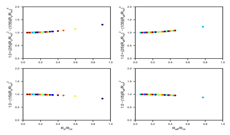
Figure 10: The terms $1-\frac{1}{5}\frac{R^{2}_{s}}{R^{2}_{g}}$ and $1+\frac{2}{5}(\frac{R_{s}}{R_{g}})^{2}-\frac{1}{35}(\frac{R_{s}}{R_{g}})^{4}$ are almost constant for most of the data points in our sub-sample of SPARC. Left: It is assumed that $R_{s}=R_{d}$ and $R_{g}=R_{HI}$. Only four data points show a noticeable deviation from one due to their relatively large $R_{d}/R_{HI}$ ratios. Right: $R_{s}=R_{eff}$. One data point shows about 25 $\%$ deviation from one; the rest show a negligible deviation.

Now, we will show that the terms in the parentheses on the RHS of both Eqs. 36 and 38 are very close to one for most objects in the SPARC sample; thus, they could be approximated as one. These are the sub-leading terms related to the particular mass distributions considered. To see this, we have plotted $1-\frac{1}{5}\frac{R^{2}_{s}}{R^{2}_{g}}$ and $1+\frac{2}{5}(\frac{R_{s}}{R_{g}})^{2}-\frac{1}{35}(\frac{R_{s}}{R_{g}})^{4}$ in Fig 10. If we assume $R_{s}=R_{d}$ and $R_{g}=R_{HI}$, then it could be seen clearly from these two plots that the variation from one is quite negligible for most objects. In fact, only four objects show a clear deviation from one. For large ratios of $R_{s}/R_{g}$, the variation from unity could be estimated as $35\%$ at most; however, for smaller ratios of $R_{s}/R_{g}$ the terms are quite close to one. The graph on the right in Fig 10 shows that a similar behavior happens when $R_{s}=R_{eff}$.

Therefore, neglecting the higher order terms, i.e. $(R_{s}/R_{g})^{n}$ with $n\geq~{}2$, the total virial energy of a general system with gaseous and stellar components could be approximated as follows

$$-W_{tot}\simeq G\left[\alpha(\frac{M^{2}_{g}}{R_{g}}+\frac{M^{2}_{s}}{R_{s}})+\gamma_{1}\frac{M_{s}M_{g}}{R_{g}}\right]+\frac{2c_{1}a_{0}}{M}\left[\beta(M^{2}_{g}R_{g}+M^{2}_{s}R_{s})+\gamma_{2}M_{s}M_{g}R_{g}\right]$$

in which $\gamma_{1}$ and $\gamma_{2}$ are two constants related to the geometry of the two systems. The terms proportional to $\gamma_{1}$ and $\gamma_{2}$ estimate the virial interaction of gas and stars up to $35\%$. This general form of $W_{tot}$ is used to derive the equilibrium radius of a compound system above. See Eq. 14 and the discussion thereafter.

Appendix C Supplementary Figures

The main results of this work are not dependent to the figures in this appendix; however, we have used these plots in some of our discussions in the manuscript. For example, Fig. 11 displays some scale length, i.e. $R_{HI}$, $R_{eff}$ and $R_{d}$, as a function of the Freeman ratio $\mathcal{R}_{F}$ while we have used $R_{eq}$ as the dynamical scale length of the systems. See also Fig. 5. Other plots have been employed to argue why we prefer $R_{eq}$ instead of other scale length and $V_{eq}=\sqrt{0.5V^{2}_{f}+\sigma^{2}_{eq}}$ instead of flat velocity $V_{f}$.

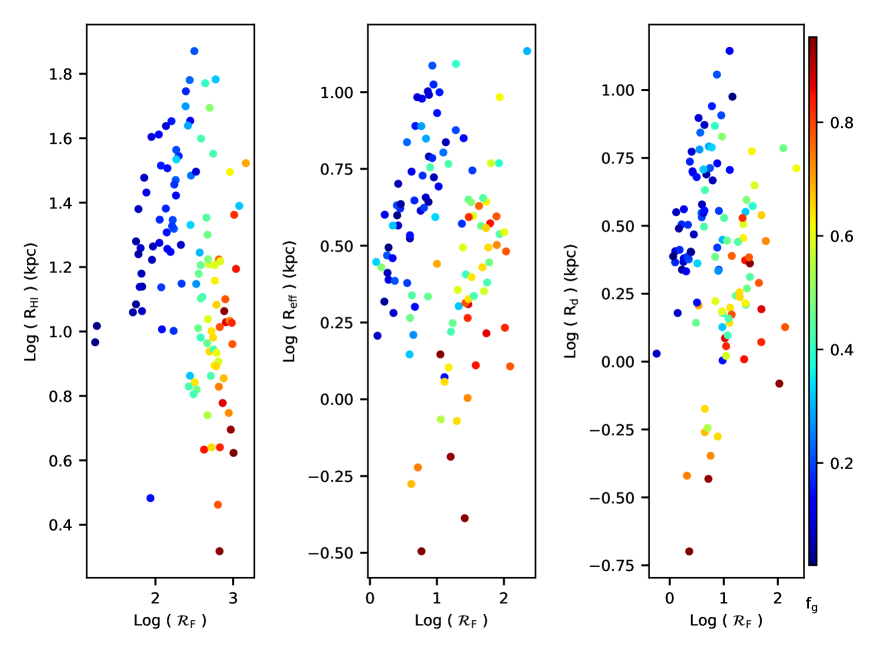
Figure 11: The change in different galactic scales ( $R_{HI},~{}R_{eff},~{}R_{d}$ ) as a function of the Freeman ratio $\mathcal{R}_{F}$. Data from SPARC (Lelli et al., 2016b, a). Color online.

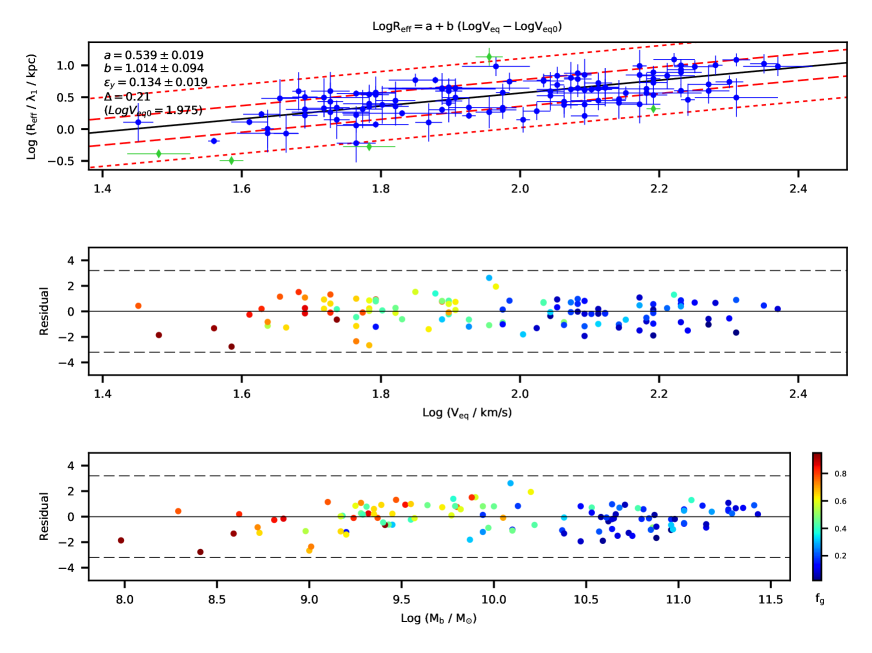
Figure 15: Data analysis of the scaling rule $R_{eff}-V_{eq}$, i.e. when the scale length of the system is $R_{eff}$ instead of $R_{eq}$, and $\sigma_{eq}=15~{}km/s$. Compare with Fig. 7. Data from SPARC (Lelli et al., 2016b, a). Color online.

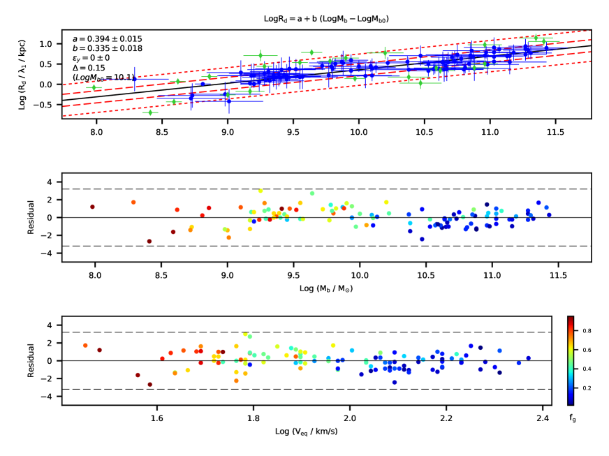
Figure 16: Data analysis of the scaling rule $R_{d}-M$, i.e. when the scale length of the system is $R_{d}$ instead of $R_{eq}$, and $\sigma_{eq}=15~{}km/s$. Compare with Fig. 6. Data from SPARC (Lelli et al., 2016b, a). Color online.

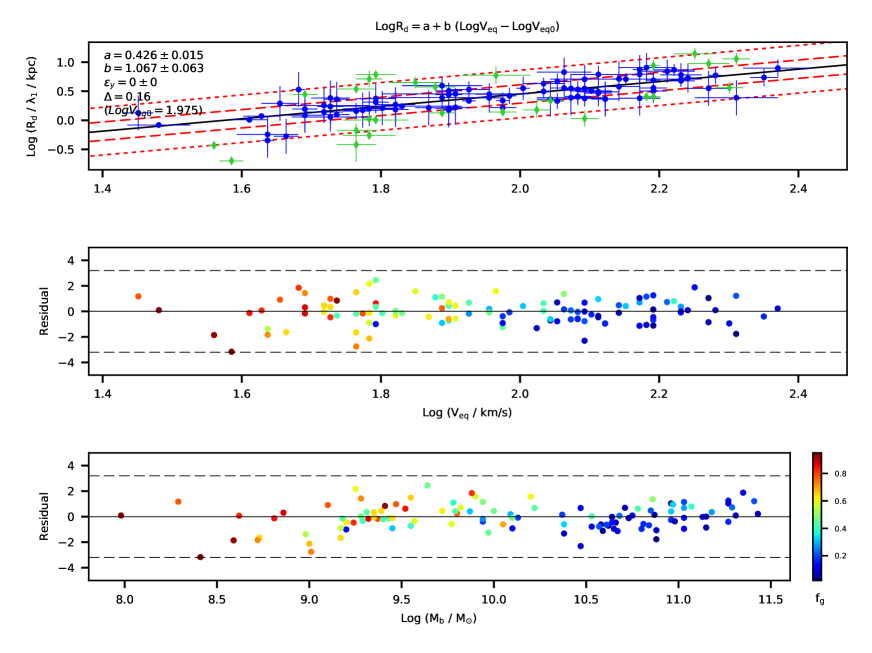
Figure 17: Data analysis of the scaling rule $R_{d}-V_{eq}$, i.e. when the scale length of the system is $R_{d}$ instead of $R_{eq}$, and $\sigma_{eq}=15~{}km/s$. Compare with Fig. 7. Data from SPARC (Lelli et al., 2016b, a). Color online.

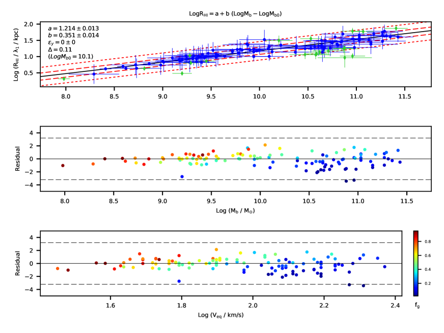
Figure 18: Data analysis of the scaling rule $R_{HI}-M$, i.e. when the scale length of the system is $R_{HI}$ instead of $R_{eq}$, and $\sigma_{eq}=15~{}km/s$. Compare with Fig. 6. Data from SPARC (Lelli et al., 2016b, a). Color online.

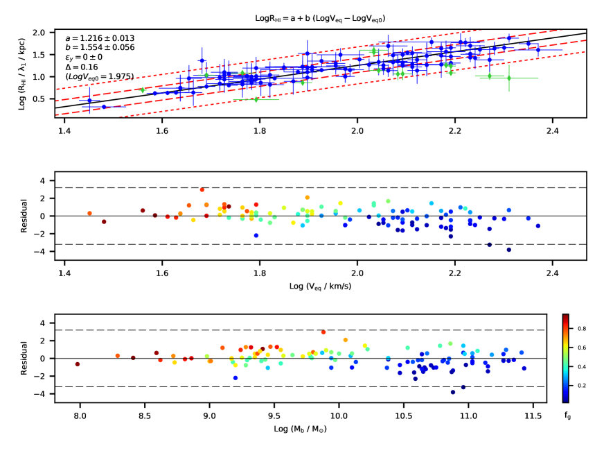
Figure 19: Data analysis of the scaling rule $R_{HI}-V_{eq}$, i.e. when the scale length of the system is $R_{HI}$ instead of $R_{eq}$, and $\sigma_{eq}=15~{}km/s$. Compare with Fig. 7. Data from SPARC (Lelli et al., 2016b, a). Color online.

References

- Agnello and Evans (2012) A. Agnello and N. W. Evans. Virial sequences for thick discs and haloes: flattening and global anisotropy. MNRAS, 422:1767–1778, May 2012. doi: 10.1111/j.1365-2966.2012.20750.x.
- Akritas and Bershady (1996) M. G. Akritas and M. A. Bershady. Linear Regression for Astronomical Data with Measurement Errors and Intrinsic Scatter. ApJ, 470:706, October 1996. doi: 10.1086/177901.
- Balakrishna Subramani et al. (2019) Vasanth Balakrishna Subramani, Pavel Kroupa, Hossein Shenavar, and Vyoma Muralidhara. Pseudo-evolution of galaxies in CDM cosmology. MNRAS, 488(3):3876–3883, Sep 2019. doi: 10.1093/mnras/stz2027.
- Behar and Carmeli (1999) Silvia Behar and Moshe Carmeli. Derivation of the Tully-Fisher Law from General Relativity Theory: Doubts about the Existence of Halo Dark Matter. arXiv e-prints, art. astro-ph/9907244, July 1999.
- Bhattacharyya and Gopalsamy (1988) PK Bhattacharyya and S Gopalsamy. On existence and uniqueness of solutions of boundary value problems of fourth order elliptic partial differential equations with variable coefficients. Journal of mathematical analysis and applications, 136(2):589–608, 1988.
- Binney and Tremaine (2008) J. Binney and S. Tremaine. Galactic Dynamics: Second Edition. Princeton University Press, 2008.
- Binney and Evans (2001) J. J. Binney and N. W. Evans. Cuspy dark matter haloes and the Galaxy. MNRAS, 327:L27–L31, October 2001. doi: 10.1046/j.1365-8711.2001.04968.x.
- Brandt (1960) J. C. Brandt. On the Distribution Of mass in Galaxies. I. The Large-Scale Structure of Ordinary Spirals with Applications to M 31. ApJ, 131:293, March 1960. doi: 10.1086/146833.
- Cappellari (2016) M. Cappellari. Structure and Kinematics of Early-Type Galaxies from Integral Field Spectroscopy. ARA & A, 54:597–665, September 2016. doi: 10.1146/annurev-astro-082214-122432.
- Cappellari et al. (2007) M. Cappellari, E. Emsellem, R. Bacon, M. Bureau, R. L. Davies, P. T. de Zeeuw, J. Falcón-Barroso, D. Krajnović, H. Kuntschner, R. M. McDermid, R. F. Peletier, M. Sarzi, R. C. E. van den Bosch, and G. van de Ven. The SAURON project - X. The orbital anisotropy of elliptical and lenticular galaxies: revisiting the (V/, ) diagram with integral-field stellar kinematics. MNRAS, 379:418–444, August 2007. doi: 10.1111/j.1365-2966.2007.11963.x.
- Cappellari et al. (2013) M. Cappellari, N. Scott, K. Alatalo, L. Blitz, M. Bois, F. Bournaud, M. Bureau, A. F. Crocker, R. L. Davies, T. A. Davis, P. T. de Zeeuw, P.-A. Duc, E. Emsellem, S. Khochfar, D. Krajnović, H. Kuntschner, R. M. McDermid, R. Morganti, T. Naab, T. Oosterloo, M. Sarzi, P. Serra, A.-M. Weijmans, and L. M. Young. The ATLAS3D project - XV. Benchmark for early-type galaxies scaling relations from 260 dynamical models: mass-to-light ratio, dark matter, Fundamental Plane and Mass Plane. MNRAS, 432:1709–1741, July 2013. doi: 10.1093/mnras/stt562.
- Carmeli (2003) Moshe Carmeli. Five-dimensional cosmological theory of unified space, time and velocity. Nuclear Physics B Proceedings Supplements, 124:258–263, July 2003. doi: 10.1016/S0920-5632(03)02118-2.
- Casertano (1983) S. Casertano. Rotation curve of the edge-on spiral galaxy NGC 5907: disc and halo masses. MNRAS, 203:735–747, May 1983. doi: 10.1093/mnras/203.3.735.
- Casertano and van Gorkom (1991) S. Casertano and J. H. van Gorkom. Declining rotation curves - The end of a conspiracy? AJ, 101:1231–1241, April 1991. doi: 10.1086/115759.
- Chae et al. (2020) Kyu-Hyun Chae, Federico Lelli, Harry Desmond, Stacy S. McGaugh, Pengfei Li, and James M. Schombert. Testing the Strong Equivalence Principle: Detection of the External Field Effect in Rotationally Supported Galaxies. ApJ, 904(1):51, November 2020. doi: 10.3847/1538-4357/abbb96.
- Chae et al. (2021a) Kyu-Hyun Chae, Harry Desmond, Federico Lelli, Stacy S. McGaugh, and James M. Schombert. Testing the Strong Equivalence Principle. II. Relating the External Field Effect in Galaxy Rotation Curves to the Large-Scale Structure of the Universe. arXiv e-prints, art. arXiv:2109.04745, September 2021a.
- Chae et al. (2021b) Kyu-Hyun Chae, Federico Lelli, Harry Desmond, Stacy S. McGaugh, Pengfei Li, and James M. Schombert. Erratum: “Testing the Strong Equivalence Principle: Detection of the External Field Effect in Rotationally Supported Galaxies” (2020, ApJ, 904, 51). ApJ, 910(1):81, March 2021b. doi: 10.3847/1538-4357/abebdc.
- Chandrasekhar and Lebovitz (1962a) S. Chandrasekhar and N. R. Lebovitz. On Super-Potentials in the Theory of Newtonian Gravitation. ApJ, 135:238, January 1962a. doi: 10.1086/147261.
- Chandrasekhar and Lebovitz (1962b) S. Chandrasekhar and N. R. Lebovitz. On Superpotentials in the Theory of Newtonian Gravitation. II. Tensors of Higher Rank. ApJ, 136:1032, November 1962b. doi: 10.1086/147455.
- Chandrasekhar and Lebovitz (1962c) S. Chandrasekhar and N. R. Lebovitz. The Potentials and the Superpotentials of Homogeneous Ellipsoids. ApJ, 136:1037, November 1962c. doi: 10.1086/147456.
- Collins (1978) G. W. Collins, II. The virial theorem in stellar astrophysics. 1978.
- Cortese et al. (2014) L. Cortese, L. M. R. Fogarty, I. T. Ho, K. Bekki, J. Bland-Hawthorn, M. Colless, W. Couch, S. M. Croom, K. Glazebrook, J. Mould, N. Scott, R. Sharp, C. Tonini, J. T. Allen, J. Bloom, J. J. Bryant, M. Cluver, R. L. Davies, M. J. Drinkwater, M. Goodwin, A. Green, L. J. Kewley, I. S. Kostantopoulos, J. S. Lawrence, S. Mahajan, A. M. Medling, M. Owers, S. N. Richards, S. M. Sweet, and O. I. Wong. The SAMI Galaxy Survey: Toward a Unified Dynamical Scaling Relation for Galaxies of All Types. ApJL, 795(2):L37, Nov 2014. doi: 10.1088/2041-8205/795/2/L37.
- Davis et al. (2019) B. L. Davis, A. W. Graham, and F. Combes. A Consistent Set of Empirical Scaling Relations for Spiral Galaxies: The (, ) - (, , ) Relations. ApJ, 877:64, May 2019. doi: 10.3847/1538-4357/ab1aa4.
- Desmond (2017) H. Desmond. The scatter, residual correlations and curvature of the SPARC baryonic Tully-Fisher relation. MNRAS, 472:L35–L39, November 2017. doi: 10.1093/mnrasl/slx134.
- Di Paolo et al. (2019) Chiara Di Paolo, Paolo Salucci, and Adnan Erkurt. The universal rotation curve of low surface brightness galaxies – IV. The interrelation between dark and luminous matter. MNRAS, 490(4):5451–5477, 09 2019. ISSN 0035-8711. doi: 10.1093/mnras/stz2700. URL https://doi.org/10.1093/mnras/stz2700.
- Ellis (2013) George Francis Rayner Ellis. The arrow of time and the nature of spacetime. Studies in the History and Philosophy of Modern Physics, 44(3):242–262, August 2013. doi: 10.1016/j.shpsb.2013.06.002.
- Faber and Jackson (1976) S. M. Faber and R. E. Jackson. Velocity dispersions and mass-to-light ratios for elliptical galaxies. ApJ, 204:668–683, March 1976. doi: 10.1086/154215.
- Famaey and McGaugh (2012) B. Famaey and S. S. McGaugh. Modified Newtonian Dynamics (MOND): Observational Phenomenology and Relativistic Extensions. Living Reviews in Relativity, 15:10, September 2012. doi: 10.12942/lrr-2012-10.
- Feigelson and Babu (2012) Eric D Feigelson and G Jogesh Babu. Modern statistical methods for astronomy: with R applications. Cambridge University Press, 2012.
- Freeman (1970) K. C. Freeman. On the Disks of Spiral and S0 Galaxies. ApJ, 160:811, Jun 1970. doi: 10.1086/150474.
- Freeman (1999) K. C. Freeman. Historical Introduction. In J. I. Davies, C. Impey, and S. Phillips, editors, The Low Surface Brightness Universe, volume 170 of Astronomical Society of the Pacific Conference Series, page 3, 1999.
- Ghosh et al. (2021) Samrat Ghosh, Arunava Bhadra, Amitabha Mukhopadhyay, and Kabita Sarkar. Baryonic Tully-Fisher Test of Grumiller’s Modified Gravity Model. Gravitation and Cosmology, 27(2):157–162, April 2021. doi: 10.1134/S0202289321020067.
- Grubbs (1969) Frank E Grubbs. Procedures for detecting outlying observations in samples. Technometrics, 11(1):1–21, 1969.
- Grumiller (2010) Daniel Grumiller. Model for Gravity at Large Distances. PhRvL, 105(21):211303, November 2010. doi: 10.1103/PhysRevLett.105.211303.
- Grumiller (2011) Daniel Grumiller. Erratum: Model for Gravity at Large Distances [Phys. Rev. Lett. 105, 211303 (2010)]. PhRvL, 106(3):039901, January 2011. doi: 10.1103/PhysRevLett.106.039901.
- Hawking and Ellis (1973) S. W. Hawking and G. F. R. Ellis. The large-scale structure of space-time. 1973.
- Holwerda et al. (2012) B. W. Holwerda, S. L. Blyth, and A. J. Baker. Looking at the distant universe with the MeerKAT Array (LADUMA). In Richard J. Tuffs and Cristina C. Popescu, editors, The Spectral Energy Distribution of Galaxies - SED 2011, volume 284, pages 496–499, August 2012. doi: 10.1017/S1743921312009702.
- Iorio et al. (2017) G. Iorio, F. Fraternali, C. Nipoti, E. Di Teodoro, J. I. Read, and G. Battaglia. LITTLE THINGS in 3D: robust determination of the circular velocity of dwarf irregular galaxies. MNRAS, 466(4):4159–4192, April 2017. doi: 10.1093/mnras/stw3285.
- Karukes and Salucci (2016) E. V. Karukes and P. Salucci. The universal rotation curve of dwarf disc galaxies. MNRAS, 465(4):4703–4722, 11 2016. ISSN 0035-8711. doi: 10.1093/mnras/stw3055. URL https://doi.org/10.1093/mnras/stw3055.
- Kassin et al. (2007) S. A. Kassin, B. J. Weiner, S. M. Faber, D. C. Koo, J. M. Lotz, J. Diemand, J. J. Harker, K. Bundy, A. J. Metevier, A. C. Phillips, M. C. Cooper, D. J. Croton, N. Konidaris, K. G. Noeske, and C. N. A. Willmer. The Stellar Mass Tully-Fisher Relation to z = 1.2 from AEGIS. ApJL, 660:L35–L38, May 2007. doi: 10.1086/517932.
- Kazanas (1995) Demosthenes Kazanas. Alternatives to dark matter. In Stephen S. Holt and Charles L. Bennett, editors, Dark Matter, volume 336 of American Institute of Physics Conference Series, pages 495–504, July 1995. doi: 10.1063/1.48382.
- Larson (1981) R. B. Larson. Turbulence and star formation in molecular clouds. MNRAS, 194:809–826, March 1981. doi: 10.1093/mnras/194.4.809.
- Lelli et al. (2016a) F. Lelli, S. S. McGaugh, and J. M. Schombert. SPARC: Mass Models for 175 Disk Galaxies with Spitzer Photometry and Accurate Rotation Curves. AJ, 152:157, December 2016a. doi: 10.3847/0004-6256/152/6/157.
- Lelli et al. (2016b) F. Lelli, S. S. McGaugh, and J. M. Schombert. The Small Scatter of the Baryonic Tully-Fisher Relation. ApJL, 816:L14, January 2016b. doi: 10.3847/2041-8205/816/1/L14.
- Lelli et al. (2017) F. Lelli, S. S. McGaugh, J. M. Schombert, and M. S. Pawlowski. One Law to Rule Them All: The Radial Acceleration Relation of Galaxies. ApJ, 836:152, February 2017. doi: 10.3847/1538-4357/836/2/152.
- Lelli et al. (2019) F. Lelli, S. S. McGaugh, J. M. Schombert, H. Desmond, and H. Katz. The baryonic Tully-Fisher relation for different velocity definitions and implications for galaxy angular momentum. MNRAS, 484:3267–3278, April 2019. doi: 10.1093/mnras/stz205.
- Leroy and Rousseeuw (1987) A. M. Leroy and P. J. Rousseeuw. Robust regression and outlier detection. 1987.
- Lin et al. (2013) Hai-Nan Lin, Ming-Hua Li, Xin Li, and Zhe Chang. Galaxy rotation curves in the Grumiller’s modified gravity. MNRAS, 430(1):450–458, March 2013. doi: 10.1093/mnras/sts642.
- Mancera Piña et al. (2019) Pavel E. Mancera Piña, Filippo Fraternali, Elizabeth A. K. Adams, Antonino Marasco, Tom Oosterloo, Kyle A. Oman, Lukas Leisman, Enrico M. di Teodoro, Lorenzo Posti, Michael Battipaglia, John M. Cannon, Lexi Gault, Martha P. Haynes, Steven Janowiecki, Elizabeth McAllan, Hannah J. Pagel, Kameron Reiter, Katherine L. Rhode, John J. Salzer, and Nicholas J. Smith. Off the Baryonic Tully-Fisher Relation: A Population of Baryon-dominated Ultra-diffuse Galaxies. ApJL, 883(2):L33, October 2019. doi: 10.3847/2041-8213/ab40c7.
- Mancera Piña et al. (2020) Pavel E. Mancera Piña, Filippo Fraternali, Kyle A. Oman, Elizabeth A. K. Adams, Cecilia Bacchini, Antonino Marasco, Tom Oosterloo, Gabriele Pezzulli, Lorenzo Posti, Lukas Leisman, John M. Cannon, Enrico M. di Teodoro, Lexi Gault, Martha P. Haynes, Kameron Reiter, Katherine L. Rhode, John J. Salzer, and Nicholas J. Smith. Robust H I kinematics of gas-rich ultra-diffuse galaxies: hints of a weak-feedback formation scenario. MNRAS, 495(4):3636–3655, July 2020. doi: 10.1093/mnras/staa1256.
- Mancera Piña et al. (2021a) Pavel E. Mancera Piña, Lorenzo Posti, Filippo Fraternali, Elizabeth A. K. Adams, and Tom Oosterloo. The baryonic specific angular momentum of disc galaxies. A & A, 647:A76, March 2021a. doi: 10.1051/0004-6361/202039340.
- Mancera Piña et al. (2021b) Pavel E. Mancera Piña, Lorenzo Posti, Gabriele Pezzulli, Filippo Fraternali, S. Michael Fall, Tom Oosterloo, and Elizabeth A. K. Adams. A tight angular-momentum plane for disc galaxies. A & A, 651:L15, July 2021b. doi: 10.1051/0004-6361/202141574.
- Mannheim (2006) Philip D. Mannheim. Alternatives to dark matter and dark energy. Progress in Particle and Nuclear Physics, 56(2):340–445, April 2006. doi: 10.1016/j.ppnp.2005.08.001.
- Mannheim and Kazanas (1989) Philip D. Mannheim and Demosthenes Kazanas. Exact Vacuum Solution to Conformal Weyl Gravity and Galactic Rotation Curves. ApJ, 342:635, July 1989. doi: 10.1086/167623.
- Mannheim and Kazanas (1994) Philip D. Mannheim and Demosthenes Kazanas. Newtonian limit of conformal gravity and the lack of necessity of the second order Poisson equation. General Relativity and Gravitation, 26(4):337–361, April 1994. doi: 10.1007/BF02105226.
- Mannheim and O’Brien (2012) Philip D. Mannheim and James G. O’Brien. Fitting galactic rotation curves with conformal gravity and a global quadratic potential. PhRvD, 85(12):124020, June 2012. doi: 10.1103/PhysRevD.85.124020.
- McGaugh (1996) S. S. McGaugh. The number, luminosity and mass density of spiral galaxies as a function of surface brightness. MNRAS, 280:337–354, May 1996. doi: 10.1093/mnras/280.2.337.
- McGaugh (2005a) S. S. McGaugh. The Baryonic Tully-Fisher Relation of Galaxies with Extended Rotation Curves and the Stellar Mass of Rotating Galaxies. ApJ, 632:859–871, October 2005a. doi: 10.1086/432968.
- McGaugh et al. (2000) S. S. McGaugh, J. M. Schombert, G. D. Bothun, and W. J. G. de Blok. The Baryonic Tully-Fisher Relation. ApJL, 533:L99–L102, April 2000. doi: 10.1086/312628.
- McGaugh et al. (2016) S. S. McGaugh, F. Lelli, and J. M. Schombert. Radial Acceleration Relation in Rotationally Supported Galaxies. Physical Review Letters, 117(20):201101, November 2016. doi: 10.1103/PhysRevLett.117.201101.
- McGaugh (2005b) Stacy S. McGaugh. Balance of Dark and Luminous Mass in Rotating Galaxies. PhRvL, 95(17):171302, Oct 2005b. doi: 10.1103/PhysRevLett.95.171302.
- Milgrom (1983a) M. Milgrom. A Modification of the Newtonian dynamics as a possible alternative to the hidden mass hypothesis. Astrophys. J., 270:365–370, 1983a. doi: 10.1086/161130.
- Milgrom (1983b) M. Milgrom. A Modification of the Newtonian dynamics: Implications for galaxies. Astrophys. J., 270:371–383, 1983b. doi: 10.1086/161131.
- Milgrom (1983c) M. Milgrom. A modification of the Newtonian dynamics: implications for galaxy systems. Astrophys. J., 270:384–389, 1983c. doi: 10.1086/161132.
- Milgrom (1989) M. Milgrom. On stability of galactic disks in the modified dynamics and the distribution of their mean surface brightness. ApJ, 338:121–127, March 1989. doi: 10.1086/167184.
- Milgrom (1999) Mordehai Milgrom. The modified dynamics as a vacuum effect. Physics Letters A, 253(5-6):273–279, March 1999. doi: 10.1016/S0375-9601(99)00077-8.
- Milgrom (2009) Mordehai Milgrom. The Mond Limit from Spacetime Scale Invariance. ApJ, 698(2):1630–1638, June 2009. doi: 10.1088/0004-637X/698/2/1630.
- Misner et al. (1973) Charles W. Misner, Kip S. Thorne, and John A. Wheeler. Gravitation. 1973.
- Mo et al. (1998) H. J. Mo, S. Mao, and S. D. M. White. The formation of galactic discs. MNRAS, 295:319–336, April 1998. doi: 10.1046/j.1365-8711.1998.01227.x.
- Moore et al. (1999) B. Moore, S. Ghigna, F. Governato, G. Lake, T. Quinn, J. Stadel, and P. Tozzi. Dark Matter Substructure within Galactic Halos. ApJL, 524:L19–L22, October 1999. doi: 10.1086/312287.
- Mosleh et al. (2012) Moein Mosleh, Rik J. Williams, Marijn Franx, Valentino Gonzalez, Rychard J. Bouwens, Pascal Oesch, Ivo Labbe, Garth D. Illingworth, and Michele Trenti. The Evolution of Mass-Size Relation for Lyman Break Galaxies from z = 1 to z = 7. ApJL, 756(1):L12, September 2012. doi: 10.1088/2041-8205/756/1/L12.
- Mowla et al. (2019) Lamiya A. Mowla, Pieter van Dokkum, Gabriel B. Brammer, Ivelina Momcheva, Arjen van der Wel, Katherine Whitaker, Erica Nelson, Rachel Bezanson, Adam Muzzin, Marijn Franx, John MacKenty, Joel Leja, Mariska Kriek, and Danilo Marchesini. COSMOS-DASH: The Evolution of the Galaxy Size-Mass Relation since z 3 from New Wide-field WFC3 Imaging Combined with CANDELS/3D-HST. ApJ, 880(1):57, July 2019. doi: 10.3847/1538-4357/ab290a.
- Navarro et al. (1996) J. F. Navarro, C. S. Frenk, and S. D. M. White. The Structure of Cold Dark Matter Halos. ApJ, 462:563, May 1996. doi: 10.1086/177173.
- Navarro et al. (1997) J. F. Navarro, C. S. Frenk, and S. D. M. White. A Universal Density Profile from Hierarchical Clustering. ApJ, 490:493–508, December 1997. doi: 10.1086/304888.
- Navarro (2018) Julio F. Navarro. The origin of galaxy scaling laws in LCDM. arXiv e-prints, art. arXiv:1811.02025, Nov 2018.
- O’Brien and Mannheim (2012) James G. O’Brien and Philip D. Mannheim. Fitting dwarf galaxy rotation curves with conformal gravity. MNRAS, 421(2):1273–1282, April 2012. doi: 10.1111/j.1365-2966.2011.20386.x.
- O’Brien et al. (2018) James G. O’Brien, Thomas L. Chiarelli, and Philip D. Mannheim. Universal properties of galactic rotation curves and a first principles derivation of the Tully-Fisher relation. Physics Letters B, 782:433–439, July 2018. doi: 10.1016/j.physletb.2018.05.060.
- Press et al. (2007) William H Press, Saul A Teukolsky, William T Vetterling, and Brian P Flannery. Numerical recipes 3rd edition: The art of scientific computing. Cambridge university press, 2007.
- Rajohnson et al. (2022) Sambatriniaina H. A. Rajohnson, Bradley S. Frank, Anastasia A. Ponomareva, Natasha Maddox, Renée C. Kraan-Korteweg, Matt J. Jarvis, Elizabeth A. K. Adams, Tom Oosterloo, Maarten Baes, Kristine Spekkens, Nathan J. Adams, Marcin Glowacki, Sushma Kurapati, Isabella Prandoni, Ian Heywood, Jordan D. Collier, Srikrishna Sekhar, and Russ Taylor. MIGHTEE-H I: the H I size-mass relation over the last billion years. MNRAS, 512(2):2697–2706, May 2022. doi: 10.1093/mnras/stac693.
- Roberts (1962) P. H. Roberts. On the Superpotential and Supermatrix of a Heterogeneous Ellipsoid. ApJ, 136:1108, November 1962. doi: 10.1086/147461.
- Romanowsky and Fall (2012) A. J. Romanowsky and S. M. Fall. Angular Momentum and Galaxy Formation Revisited. ApJS, 203:17, December 2012. doi: 10.1088/0067-0049/203/2/17.
- Romeo (2020) Alessandro B. Romeo. From massive spirals to dwarf irregulars: a new set of tight scaling relations for cold gas and stars driven by disc gravitational instability. MNRAS, 491(4):4843–4851, February 2020. doi: 10.1093/mnras/stz3367.
- Romeo and Mogotsi (2018) Alessandro B. Romeo and Keoikantse Moses Mogotsi. Angular momentum and local gravitational instability in galaxy discs: does Q correlate with j or M ? MNRAS, 480(1):L23–L27, October 2018. doi: 10.1093/mnrasl/sly119.
- Romeo et al. (2020) Alessandro B. Romeo, Oscar Agertz, and Florent Renaud. From lenticulars to blue compact dwarfs: the stellar mass fraction is regulated by disc gravitational instability. MNRAS, 499(4):5656–5664, December 2020. doi: 10.1093/mnras/staa3245.
- Rousseeuw (1984) Peter J Rousseeuw. Least median of squares regression. Journal of the American statistical association, 79(388):871–880, 1984.
- Rousseeuw and Van Driessen (2006) Peter J Rousseeuw and Katrien Van Driessen. Computing lts regression for large data sets. Data mining and knowledge discovery, 12(1):29–45, 2006.
- Saintonge and Spekkens (2011) A. Saintonge and K. Spekkens. Disk Galaxy Scaling Relations in the SFI++: Intrinsic Scatter and Applications. ApJ, 726:77, January 2011. doi: 10.1088/0004-637X/726/2/77.
- Salucci (2019) Paolo Salucci. The distribution of dark matter in galaxies. Astron. Astrophys. Rev., 27(1):2, February 2019. doi: 10.1007/s00159-018-0113-1.
- Sanders (2010) R. H. Sanders. The Dark Matter Problem: A Historical Perspective. April 2010.
- Schulz (2017) Earl Schulz. Scaling Relations of Mass, Velocity, and Radius for Disk Galaxies. ApJ, 836(2):151, Feb 2017. doi: 10.3847/1538-4357/aa5b88.
- Secco (2000) L. Secco. Double gravitational bound system in virial equilibrium: tidal scale length induced on one subsystem by another. New Astron., 5:403–421, November 2000. doi: 10.1016/S1384-1076(00)00040-3.
- Secco (2001) L. Secco. The Fundamental Plane as a consequence of Clausius’ virial minimum. New Astron., 6:339–357, September 2001. doi: 10.1016/S1384-1076(01)00064-1.
- Selvadurai (2013) Antony PS Selvadurai. Partial differential equations in mechanics 2: the biharmonic equation, Poisson’s equation. Springer Science & Business Media, 2013.
- Shenavar (2016a) Hossein Shenavar. Imposing Neumann boundary condition on cosmological perturbation equations and trajectories of particles. Astrophys. Space Sci., 361(3):93, 2016a. doi: 10.1007/s10509-016-2676-5.
- Shenavar (2016b) Hossein Shenavar. Motion of particles in solar and galactic systems by using Neumann boundary condition. Astrophys. Space Sci., 361(12):378, 2016b. doi: 10.1007/s10509-016-2964-0.
- Shenavar (2022) Hossein Shenavar. Three-Body Problem in Modified Dynamics. arXiv e-prints, art. arXiv:2205.02281, May 2022. doi: 10.48550/arXiv.2205.02281.
- Shenavar and Ghafourian (2018) Hossein Shenavar and Neda Ghafourian. Local stability of galactic discs in modified dynamics. MNRAS, 475(4):5603–5617, 2018.
- Shenavar and Javidan (2020) Hossein Shenavar and Kurosh Javidan. A Modified Dynamical Model of Cosmology I. Theory. Universe, 6(1):arXiv:1810.05001, Jan 2020. doi: 10.3390/universe6010001.
- Thorne et al. (1973) Kip S. Thorne, David L. Lee, and Alan P. Lightman. Foundations for a Theory of Gravitation Theories. PhRvD, 7(12):3563–3578, June 1973. doi: 10.1103/PhysRevD.7.3563.
- Toomre (1963) A. Toomre. On the Distribution of Matter Within Highly Flattened Galaxies. ApJ, 138:385, August 1963. doi: 10.1086/147653.
- Tremaine et al. (2002) S. Tremaine, K. Gebhardt, R. Bender, G. Bower, A. Dressler, S. M. Faber, A. V. Filippenko, R. Green, C. Grillmair, L. C. Ho, J. Kormendy, T. R. Lauer, J. Magorrian, J. Pinkney, and D. Richstone. The Slope of the Black Hole Mass versus Velocity Dispersion Correlation. ApJ, 574:740–753, August 2002. doi: 10.1086/341002.
- Tully and Fisher (1977) R. B. Tully and J. R. Fisher. A new method of determining distances to galaxies. A & A, 54:661–673, February 1977.
- Übler et al. (2017) H. Übler, N. M. Förster Schreiber, R. Genzel, E. Wisnioski, S. Wuyts, P. Lang, T. Naab, A. Burkert, P. G. van Dokkum, L. J. Tacconi, D. J. Wilman, M. Fossati, J. T. Mendel, A. Beifiori, S. Belli, R. Bender, G. B. Brammer, J. Chan, R. Davies, M. Fabricius, A. Galametz, D. Lutz, I. G. Momcheva, E. J. Nelson, R. P. Saglia, S. Seitz, and K. Tadaki. The Evolution of the Tully-Fisher Relation between z 2.3 and z 0.9 with KMOS3D. ApJ, 842(2):121, June 2017. doi: 10.3847/1538-4357/aa7558.
- van der Wel et al. (2014) A. van der Wel, M. Franx, P. G. van Dokkum, R. E. Skelton, I. G. Momcheva, K. E. Whitaker, G. B. Brammer, E. F. Bell, H. W. Rix, S. Wuyts, H. C. Ferguson, B. P. Holden, G. Barro, A. M. Koekemoer, Yu-Yen Chang, E. J. McGrath, B. Häussler, A. Dekel, P. Behroozi, M. Fumagalli, J. Leja, B. F. Lundgren, M. V. Maseda, E. J. Nelson, D. A. Wake, S. G. Patel, I. Labbé, S. M. Faber, N. A. Grogin, and D. D. Kocevski. 3D-HST+CANDELS: The Evolution of the Galaxy Size-Mass Distribution since z = 3. ApJ, 788(1):28, June 2014. doi: 10.1088/0004-637X/788/1/28.
- Weber and de Boer (2010) M. Weber and W. de Boer. Determination of the local dark matter density in our Galaxy. A & A, 509:A25, January 2010. doi: 10.1051/0004-6361/200913381.
- Weiner et al. (2006) B. J. Weiner, C. N. A. Willmer, S. M. Faber, J. Melbourne, S. A. Kassin, A. C. Phillips, J. Harker, A. J. Metevier, N. P. Vogt, and D. C. Koo. A Survey of Galaxy Kinematics to z~1 in the TKRS/GOODS-N Field. I. Rotation and Dispersion Properties. ApJ, 653:1027–1048, December 2006. doi: 10.1086/508921.
- Wheeler (1964) John A Wheeler. Mach’s principle as boundary condition for einstein’s equations. Gravitation and relativity, pages 303–349, 1964.
- White (1997) S. D. M. White. The Physical Origin of Galaxy Scaling Relations. In Luiz N. da Costa and Alvio Renzini, editors, Galaxy Scaling Relations: Origins, Evolution and Applications, page 3, Jan 1997.