Incorporating Residual and Normalization Layers
into Analysis of Masked Language Models
Goro Kobayashi1
Tatsuki Kuribayashi1,2
Sho Yokoi1,3
Kentaro Inui1,3 1 Tohoku University
2 Langsmith Inc.
3 RIKEN
goro.koba@dc.tohoku.ac.jp {kuribayashi, yokoi, inui}@tohoku.ac.jp
Abstract
Transformer architecture has become ubiquitous in the natural language processing field.
To interpret the Transformer-based models, their attention patterns have been extensively analyzed.
However, the Transformer architecture is not only composed of the multi-head attention; other components can also contribute to Transformers’ progressive performance.
In this study, we extended the scope of the analysis of Transformers from solely the attention patterns to the whole attention block, i.e., multi-head attention, residual connection, and layer normalization.
Our analysis of Transformer-based masked language models shows that the token-to-token interaction performed via attention has less impact on the intermediate representations than previously assumed.
These results provide new intuitive explanations of existing reports; for example, discarding the learned attention patterns tends not to adversely affect the performance.
The codes of our experiments are publicly available.111https://github.com/gorokoba560/norm-analysis-of-transformer
1 Introduction
Transformer architecture (Vaswani et al., 2017) has advanced the state of the art in a wide range of natural language processing (NLP) tasks Devlin et al. (2019); Liu et al. (2019); Lan et al. (2020).
Along with this, Transformers have become a major subject of research from the viewpoints of engineering Rogers et al. (2020) and scientific studies Merkx and Frank (2021); Manning et al. (2020).
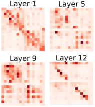
(a)
Existing analysis focusing only on the multi-head attention Kobayashi et al. (2020).
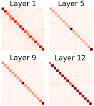
(b)
Proposed method incorporating the whole attention block (i.e., multi-head attention, residual connection, and layer normalization) into the analysis.
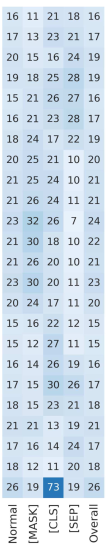
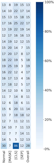
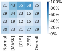
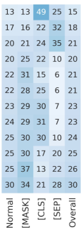
Figure 1:
Visualizations of the token-by-token interactions in each layer when a sentence pair is fed into the pre-trained BERT-base.
The diagonal elements correspond to the effect of preserving the original input information.
The contrast between Figures 1 and 1 demonstrates that the contextual information contributed less to the computation of the output representations than previously expected.
In particular, the multi-head attention, a core component of Transformers, has been extensively analyzed Clark et al. (2019); Kovaleva et al. (2019); Reif et al. (2019); Lin et al. (2019); Mareček and Rosa (2019); Htut et al. (2019); Raganato and Tiedemann (2018); Tang et al. (2018).
While these analyses suggest that the multi-head attention contributes to capturing linguistic information such as semantic and syntactic relations,
some reports question the importance of attention.
For example, several studies in fields ranging from NLP Michel et al. (2019); Kovaleva et al. (2019) to neuroscience Toneva and Wehbe (2019) empirically found that discarding learned attention patterns from Transformers retains or even improves their performance in downstream tasks and the ability to simulate human brain activity.
These observations imply that Transformers do not heavily rely on the multi-head attention alone, and the other components contribute to their progressive performance.
In this study, we broaden the scope of the analysis from the multi-head attention to the whole attention block, i.e., the multi-head attention, residual connection, and layer normalization. Our analysis of the Transformer-based masked language models Devlin et al. (2019); Liu et al. (2019)
revealed that the newly incorporated components have a larger impact than expected in previous studies Abnar and Zuidema (2020); Kobayashi et al. (2020) (Figure 1).
More concretely, we introduce an exact decomposition of the operations in the whole attention block exploiting the norm-based analysis Kobayashi et al. (2020). Our analysis quantifies the impact of the two contrasting effects of the attention block : (i) “mixing” the input representations via attention and (ii) “preserving” the original input mainly via residual connection (Section 3). Our analysis reveals that the preserving effect is more dominant in each attention block than previously estimated Abnar and Zuidema (2020); Kobayashi et al. (2020).
The results also reveal the detailed mechanism of each component in the attention block.
The residual connections pass through much larger vectors than the vectors produced by the multi-head attention.
The layer normalization also reduces the effect of the operation via attention.
Our finding of the relatively small impact of the multi-head attention provides new intuitive interpretations for some existing reports, for example, discarding the learned attention patterns did not adversely affect their performance.
Our analysis also provides a new intuitive perspective on the behaviors of Transformer-based masked language models.
For example, BERT Devlin et al. (2019) highlights low-frequency (informative) words in encoding texts, which is consistent with the existing methods for effectively computing text representations Luhn (1958); Arora et al. (2017).
The contributions of this study are as follows:
•
We expanded the scope of Transformers analysis from the multi-head attention to the attention block (i.e., multi-head attention, residual connection, and layer normalization).
•
Our analysis revealed that the operation via residual connection and layer normalization contributes more to the internal representations than expected in previous studies Abnar and Zuidema (2020); Kobayashi et al. (2020).
•
We detailed the functioning of BERT: (i) BERT tends to mix a relatively large amount of contextual information into [MASK] in the middle and later layers;
and
(ii) the contribution of contextual information in the attention block is related to word frequency.
2 Background: Transformer architecture
The Transformer architecture consists of a stack of layers.
Each layer has an attention block, which is responsible for capturing the interactions between input tokens.
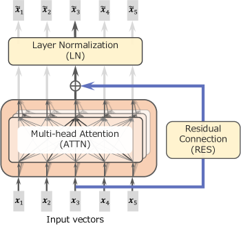
The attention block can be further divided into the three components: multi-head attention (ATTN), residual connection (RES), and layer normalization (LN) (Figure 2).
This block can be written as the following composite function:
(1)
where
is the -th input representation,
is the sequence of input representations, and
is the output representation corresponding to .
Boldface letters such as denote row vectors.
In the following, we review the computations in the ATTN, RES, and LN components.
Figure 2: Visualization of the attention block, consisting of multi-head attention, residual connection, and layer normalization, in the Transformer layer.
Multi-head attention (ATTN):
The ATTN takes the role of mixing contextual information into output representations.
Formally, given input representations , the head ATTN computes the output for each input :
(2)
where
denotes the output vector from each attention head .
is computed by each attention head as follows:
(3)
(4)
(5)
(6)
where , and are the weight matrices, and , and are the bias vectors.
denotes the dimension of each head ( is usually used), and holds.
Here, , , and stand for Query, Key, and Value, respectively.
Note that in a typical attention analysis, the attention weight has been assumed to represent the contribution of the input to computing .
Residual connection (RES):
In RES, the original input vector for the multi-head attention () is added to its output vector:
(7)
Layer normalization (LN):
LN first normalizes the input vector and then applies a transformation with learnable parameters and :
(8)
where and denote the element-wise mean and standard deviation222
Specifically, and , where denotes the -th element of the vector and is a small constant to stabilize the value.
, respectively.
Here, subtraction and division are also performed on an element-wise basis.
The normalized vector, , is then transformed with and ; here, denotes the element-wise multiplication.
Note that analyzing the feed-forward networks in each layer is beyond the scope of this study and will be carried out as future work.
3 Proposal: Analyzing attention blocks
For analyzing Transformers, solely observing the attention weights has been a common method (Clark et al., 2019; Kovaleva et al., 2019, etc.).
We extend the scope of analysis to the whole attention block (ATTN, RES, and LN).
3.1 Strategy: Norm-based analysis
Kobayashi et al. (2020) introduced the norm-based analysis to extend the scope of analysis from the attention weights to the whole multi-head attention.
We follow this norm-based analysis and extend its scope to the whole attention block.
The norm-based analysis first attempts to decompose the output vector into the sum of the transformed input vectors :
(9)
where is an appropriate vector-valued function.
Then, the contribution of to
can be expressed by the norm of .
In the next subsection, we indicate that this norm-based method can be applied to analyzing the whole attention block.
In other words, the output of the attention block is also be decomposed into the sum of the transformed input vectors without any approximation.
3.2 Decomposing output into a sum of inputs
The output is decomposed into a sum of terms associated with each input .
First, ATTN (Equation 2) can be decomposed into a sum of vectors Kobayashi et al. (2020):
(10)
(11)
Second, in RES, no interaction between subscripts and occurs, and the form is already additively decomposed.
Third, by exploiting the linearity of , we can derive the “distributive law” of LN and decompose it.
Let be the input to LN.
Then,
With these decompositions of ATTN and LN, the output of the whole attention block can be written as the sum of vector-valued functions with each input vector in as an argument:
(14)
(15)
(16)
(17)
3.3 Measuring the contribution of context
Regarding the success of the contextualized representations in NLP,
an interesting issue is the location and strength of the context mixing performed in the model.
Based on this issue, we investigate the attention block by categorizing the terms in Equation 16 into the two effects:333
The bias affects neither the context-mixing effect nor the preserving effect. Thus, we ignored this term in our analysis.
1.
Mixing contextual information into the output representation by the ATTN:
We measure the magnitude of this context-mixing effect by the norm
.
This strength refers to the amount of information from the surrounding contexts
in calculating
.
2.
Preserving the original information via ATTN and RES:
We measure the magnitude of the preserving effect by the norm .
This strength refers to the amount of information from the original vector used in calculating .
At the attention block, information from the input vector can flow through two ways: (i) attention to the original input (the first term)
and (ii) residual connection (the second term).
To summarize the relative strength of the context-mixing effect, the context-mixing ratio is defined as follows:
(18)
A higher mixing ratio indicates that the mixing effect is more dominant than the preserving effect in the computation of .
Note that Abnar and Zuidema (2020) assumed that
the multi-head attention and residual connection always equally impact the output, i.e., in the analysis of Transformers.
However, our experiments revealed that, in practical masked language models, the mixing ratio is considerably below .
4 Experiments: Analysis of mixing ratio
The context-mixing ratio of the attention blocks in pre-trained masked language models was analyzed using the proposed norm-based analysis.
The obtained results were different from those of the existing methods that analyze only some of the components in the attention block.
4.1 General setup
Model:
We investigated the 32 variants of the masked language models (BERT with five different sizes, BERT-base trained with 25 different seeds, and RoBERTa with two different sizes). In Section 4, the results for BERT-base and RoBERTa-base are demonstrated.
The results for the other models are provided in Appendix B and C.
Note that most of our findings reported in this section generalize across these model variants.
Exceptions are discussed in the relevant section (Section 4.4).
Data:
We experimented with the following four datasets:
(i) Wikipedia Clark et al. (2019), (ii) the Stanford Sentiment Treebank v2 dataset (SST-2, Socher et al., 2013), (iii) the Multi-Genre Natural Language Inference corpus (MNLI, Williams et al., 2018), and (iv) the standard CoNLL-2003 Named Entity Recognition dataset (CoNLL’03-NER, Tjong Kim Sang and
De Meulder, 2003).
The statistics of the datasets are shown in Table 1.
Owing to the limitation of space, we only give the results for the Wikipedia data in Section 4.
The trends observed for the Wikipedia dataset were generalized across the other datasets (see Appendix B).
Note that each sequence of the Wikipedia dataset consists of paired consecutive paragraphs.
Each sequence is fed into the models with masking applied to % of tokens % of the time.444
For the other datasets, we used 1000 samples from their validation set or used all of their validation set if the number of sequences is less than 1000.
Data
#Samples
Avg. length
Domains
Wikipedia
992
122
Web encyclopedia
SST-2
872
25
Movie reviews
MNLI
1000
39
10 distinct genres
CoNLL’03-NER
1000
21
News
Table 1:
Details of the datasets. Avg. length is the number of tokens segmented by BERT per sample.
Analysis methods:
We compared the context-mixing ratio computed with the following five analyzing methods:
•
Attn-w: Analyzing ATTN via attention weights, which has been applied in many existing studies (Clark et al., 2019; Kovaleva et al., 2019; Mareček and Rosa, 2019, etc.).
The ratio, where attention weight assigned to the
original input vector corresponds to the preserving effect, and the others correspond to the mixing effect, is calculated as follows:
•
Attn-n: Analyzing ATTN via the vector norm Kobayashi et al. (2020).
The mixing ratio is calculated as
•
AttnRes-w: Analyzing ATTN and RES via attention weights, as Abnar and Zuidema (2020) did.
They assumed that the residual-aware attention matrix is constructed as .
Here, is the actual attention matrix and is the identity matrix considered as the effect of residual connection.
The mixing ratio is calculated as
•
AttnRes-n (proposed): Analyzing ATTN and RES via the vector norm – a version of our proposed method that does not consider LN.
The mixing ratio is calculated as
•
AttnResLn-n (proposed): Analyzing ATTN, RES, and LN via the vector norm – the method proposed in Section 3.
This corresponds to the in Equation 18.
4.2 Results
Methods
Mean
Max
Min
— BERT-base —
Attn-w
97.1
100.0
45.0
Attn-n
85.2
100.0
4.9
AttnRes-w
48.6
50.0
22.5
AttnRes-n
22.3
65.7
2.0
AttnResLn-n
18.8
61.3
1.3
— RoBERTa-base —
Attn-w
95.8
100.0
3.8
Attn-n
84.4
100.0
13.8
AttnRes-w
47.9
50.0
1.9
AttnRes-n
19.6
69.9
1.8
AttnResLn-n
16.2
73.4
1.5
Table 2: Mean, maximum, and minimum values of the mixing ratio computed with each method.
We computed the mixing ratio of each token in each layer (each attention block) of the models with the five analysis methods (Section 4.1).
The average, maximum, and minimum mixing ratios are shown in Table 2.
Each row corresponds to a different analysis method.
Lower mixing ratio than in existing methods:
Table 2 shows that the mixing ratios obtained from the proposed AttnRes-n and AttnResLn-n largely differ from those obtained from the existing methods.
Whereas the attention analyses (Attn-w and Attn-n) yield mixing ratios of – and AttnRes-w yields –%, our proposed method (AttnResLn-n) yields about and on average.
The visualizations of the token-by-token interactions in the common attention map style become almost diagonal patterns (Figure 1).
These demonstrate that each layer’s context mixing is lower than previously expected, and RES and LN largely cancel the mixing by ATTN.
Observing the only ATTN and making an inference about the Transformer layer may lead to misleading.
Note that Srivastava et al. (2015) reported a similar trend that stacked feed-forward networks tend to prioritize the “preserving” effect in skip connections.
Consistent trends across model sizes:
Our method consistently shows the lowest mixing ratio among the compared methods for BERT and RoBERTa models of various sizes (BERT-large, medium, small, tiny, and RoBERTa-large) (Appendix B).
Interestingly, the context-mixing ratio is higher in the models with fewer layers ( in BERT-tiny, but in BERT-large).
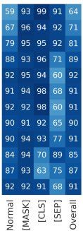
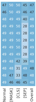
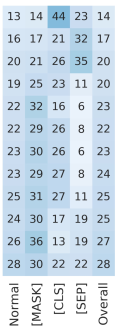
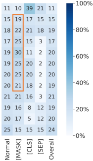
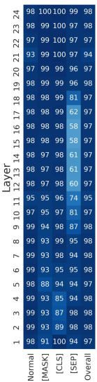
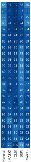
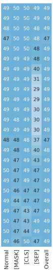
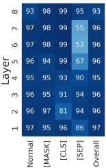
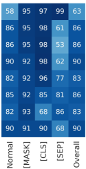
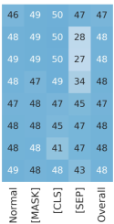
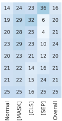
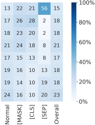
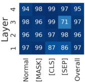
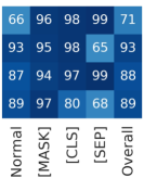
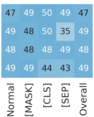
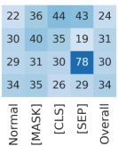
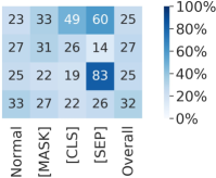
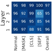
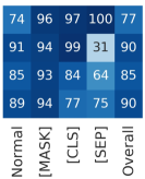
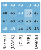
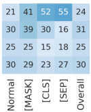
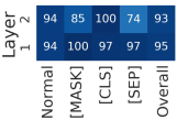
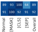
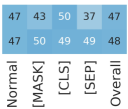
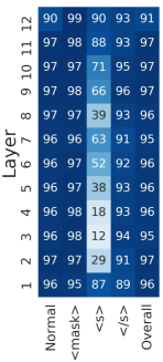
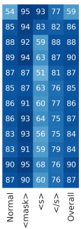
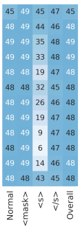
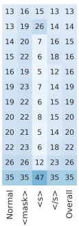
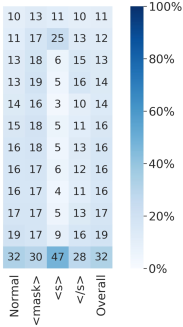
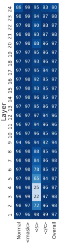
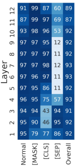
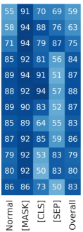
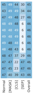
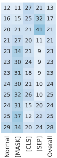
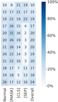
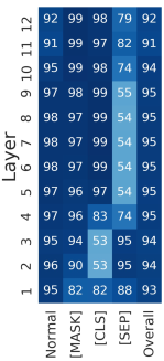
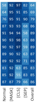
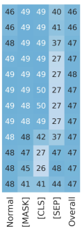
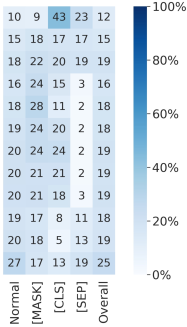
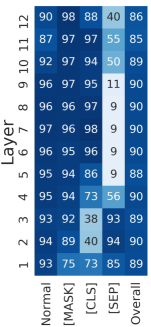
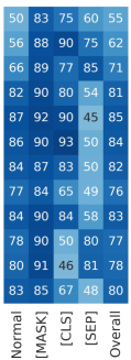
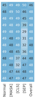
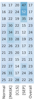
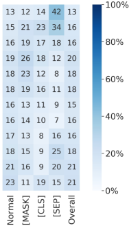
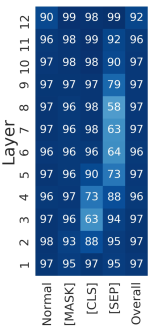
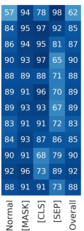
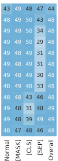
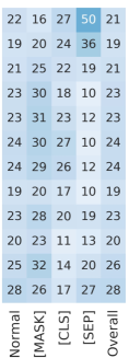
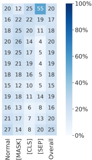
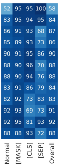
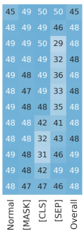
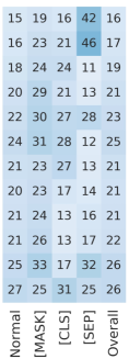
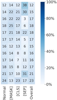
Figure 3:
Mixing ratio in each layer of BERT calculated from each method.
4.3 Connections to previous studies
Our finding of a lower mixing ratio than previously thought provides explanations for previous results and is consistent with the pre-training strategy.
Token identifiability:
The low context-mixing ratio is consistent with Brunner et al. (2020)’s reports on what they called “token identifiability.”
They showed that input tokens can be well predicted only from the corresponding internal representations within BERT, especially in shallower layers,
suggesting that context mixing is performed little by little.
Our analysis results of the whole attention block were consistent with this finding.
Masked language modeling objective:
Regarding the masked token prediction task555For masked language modeling in BERT and RoBERTa pre-training, of the tokens are randomly chosen from the input sequence, of which are replaced with [MASK], are replaced with random words, and are kept unchanged.
during the pre-training, BERT and RoBERTa learn to conduct the following operations for a given input sequence: (i) infilling the [MASK] with plausible words,
(ii) replacing the normal (non-special) tokens that might not fit their context (i.e., randomly replaced tokens) with plausible one, and (iii) reconstructing the original input tokens that might fit their context.
In our experiments and in common practical use, most tokens in the input sequence are not masked and fit their context.
Thus, BERT is assumed to reconstruct the inputs for these tokens (i.e., behave as an auto-encoder).
From this point of view, the superiority of the preserving effect is the intuitive behaviors of the masked language models.
Low impact of discarding learned attention patterns:
Several studies have reported the low impact of discarding the learned attention patterns in Transformers.
Michel et al. (2019) and Kovaleva et al. (2019) reported that the attention patterns of many attention heads in Transformers can be removed or overwritten into the uniform patterns with almost no change in their performance, and this even brought about improvements in some cases.
Voita et al. (2019) also reported the same phenomenon using a pruning method with additional training.
In addition, Toneva and Wehbe (2019) reported that using uniform attention in early layers of BERT instead of the learned attention patterns leads to a better ability to simulate human brain activity.
Our analysis shows that most of the attention signal is reduced by the immediately following modules, RES and LN.
This fact may explain the above observations that discarding the learned attention patterns of many attention heads does not cause a severe difference.
4.4 Mechanism
How is the mixing effect conducted in multi-head attention largely suppressed in the whole attention block?
We discuss the mechanism role of ATTN and LN in suppressing the mixing ratio.
ATTN reduces context-mixing ratio:
RES is a mechanism that equally adds together the output of ATTN and the input in a one-to-one fashion (Equation 7).
Considering this, the mixing ratio in the scope of ATTN and RES is expected to be about , while the mixing ratio was actually substantially below (– in AttnRes-n) (Section 4.2).
This suggests that the output of ATTN is much smaller than the input;
in other words, ATTN seems to have the effect of largely shrinking inputs to compute the output.
How is this achieved?
Recall that the output of ATTN is a weighted sum of the affine-transformed vector using with attention weight (Equation 10).
We describe and empirically show that (i) the affine transformation in ATTN has the effect of shrinking the inputs, and (ii) the attention weights and affine-transformed vectors cancel each other out on specific vectors.
We describe a brief idea here and provide the detailed derivation of each equation in the Appendix C.
First, under a coarse assumption, multiple affine transformations performed in the multi-head attention can be integrated into a single one:
(19)
Assume that the input vector is a sample from the standard normal distribution:
.
Then we can estimate its magnitude by and the magnitude after affine transformation by ,
where denote singular values of .
Thus, the expansion rate of
is approximately estimated by
(20)
If the ratio is lower than one, has a tendency of shrinking the input.
For commonly used large models, results stably demonstrated the shrinking tendency (layer mean of the expansion rate was for BERT-base and for BERT-large).
Note that, for smaller models, results demonstrated the expanding tendency (layer mean for BERT-mini and for BERT-tiny).
This is consistent with the result that the latter models tended to have a higher mixing ratio than the former models (Section 4.2).
Detailed results are shown in Appendix C.3.
Furthermore, attention weight boosts the shrinking effect.
Kobayashi et al. (2020) reported the negative correlation between and on frequent tokens.
That is, ATTN wastes a lot of attention weights by assigning them to small vectors .
To summarize, ATTN’s shrinking effect is probably achieved by (i) the shrinking in alone and (ii) further shrinking through the cancellation of and .
By these mechanisms, ATTN can contribute to decreasing the mixing ratio.
LN reduces the context-mixing ratio:
LN contains not only the vector normalization but also the affine transformation with learnable parameters (Equation 8).
Although the validity or usage of LN has been investigated in terms of stability and speed of training Parisotto et al. (2020); Liu et al. (2020), the effects of affine transformation have rarely been explored. By comparing the mixing ratios obtained from AttbRes-n and AttnResLn-n
(Table 2), we discovered that LN reduced the context-mixing ratio.
This suggests that the scaling (by ) of the affine transformation shrinks the vector from ATTN and emphasizes RES over ATTN.
5 Detailed analysis
We further analyzed the mixing ratio of the masked language models in detail from the perspectives of both the layer and word attributes.
In this section, we inherit the experimental setup (Section 4.1) from the previous section and demonstrate results for BERT-base with the Wikipedia dataset.
The results for the other experimental settings are shown in Appendix B and D.
Note that only the finding reported in Section 5.2 did not generalize across model variants, and we exceptionally discuss this point in the body.
5.1 Differences by layers and token types
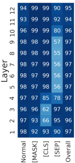
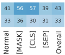
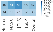
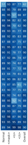
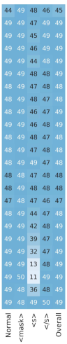
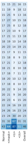
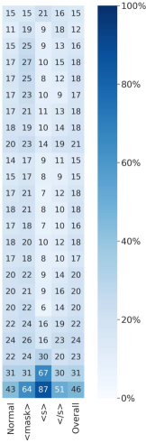
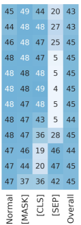
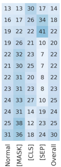
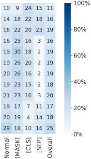
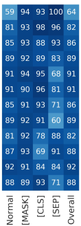
Figure 3 shows the mixing ratio in each layer
of the BERT model (results for other models are shown in Appendix B).
Each subfigure corresponds to a different analysis method, each row represents a layer, and each column represents a token type.
The averaged results of the following token categories and their overall average (“overall”) are reported: (i) non-special tokens (“normal”), (ii) [MASK], (iii) [CLS], and (iv) [SEP].
Results and discussion:
Our proposed method showed that the mixing ratio is higher in the earlier layers than in the later ones (see the “overall” trend in Figure 3).666
The Spearman’s between the “overall” mixing ratio and the layer depth are and in “overall” of BERT-base and RoBERTa-base, respectively.
This trend mirrors the tendency that a deep neural network with “gates” similar to residual connections passes through the input more in the later layers Srivastava et al. (2015).
Furthermore, our method showed a distinctive trend for the [MASK] tokens.
In the middle and deep layers, the mixing ratio for [MASK] becomes higher (–) than the overall trends (–).
Note that this trend becomes clearer when considering the RES and LN.
This trend implies that in the middle and deep layers, BERT refers to contextual information for predicting the masked words.
The trends of the other masked language models are shown in Appendix B.
Methods
Spearman’s
all tokens
w/o special tokens
Attn-w
Attn-n
AttnRes-w
AttnRes-n
AttnResLn-n
Table 3:
Spearman’s between the frequency rank and the mixing ratio calculated by each method.
In the “w/o special tokens” setting, it was calculated without [CLS] and [SEP].
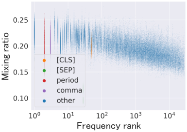
Figure 4:
Relationship between the frequency rank of tokens and the mixing ratio calculated with the AttnResLn-n.
5.2 Word frequency and mixing ratio
In this section, we will discuss the property of BERT related to the word frequency.777
Following Kobayashi et al. (2020), we counted the frequency for each word type by reproducing the training data of BERT.
Results:
Table 3 lists the Spearman’s rank correlation between the frequency rank
(e.g., , , etc.) and the mixing ratio across tokens in the text data.
The results obtained from AttnRes-n and AttnResLn-n indicate a surprisingly stronger negative correlation than the results obtained by the existing methods (Figure 4).
This indicates that BERT discounts the information of high-frequency words compared with low-frequency ones.888
Kobayashi et al. (2020) reported that ATTN in BERT tends to discounts frequent words when mixing contexts.
We found even stronger trends after broadening the scope of analysis.
Discussion:
Discounting high-frequency words is a common practice for making the semantic representation of a sentence or a text from word representations; examples are Luhn’s heuristic in classical text summarization Luhn (1958) and the smooth inverse frequency (SIF) weighting in sentence vector generation Arora et al. (2017).
Our frequency-based results reveal that attention blocks in BERT achieve this desirable property.
Our observation may also explain the phenomenon that adding up BERT’s internal or output representations does not produce a good sentence vector Reimers and Gurevych (2019).
In contrast, in static word embeddings (e.g., word2vec Mikolov et al. (2013)), the norm encodes the word importance derived from its frequency Schakel and Wilson (2015);
we can generate a good sentence vector by simply adding these static word vectors Yokoi et al. (2020).
Our finding suggests that BERT encodes the token’s importance through the context-mixing ratio rather than the norm.999
In BERT, it may be difficult for the norm to encode the token importance, because the norm is fixed at each layer normalization.
In this sense, it is plausible that additive composition using BERT’s internal or output representations does not perform well.
Generalizability:
Contrary to the other experimental results, only the relationship between word frequency and mixing ratio (Figure 4) was not consistent across different model sizes.
For the larger variant (BERT-large), a stronger negative correlation between them was indicated than for BERT-base, while for the smaller variants (BERT-medium, BERT-small, BERT-mini, and BERT-tiny), even a positive correlation or no correlation was indicated (see Appendix D).
Generally, larger BERT models (BERT-base and BERT-large) achieve better performance on downstream tasks. The different results across model sizes suggest that this desirable property can be learned when the representational power is sufficient.
6 Related work
6.1 Probing Transformers
As current neural-based models have an end-to-end, black-box nature, existing studies have adopted several strategies to interpret their inner workings Carvalho et al. (2019); Rogers et al. (2020); Braşoveanu and Andonie (2020).
In analyzing Transformers, previous studies have mainly employed the following approaches: (i) observing the vanilla attention weights Clark et al. (2019); Kovaleva et al. (2019); Reif et al. (2019); Lin et al. (2019); Mareček and Rosa (2019); Htut et al. (2019); Raganato and Tiedemann (2018); Tang et al. (2018) or the extended version Brunner et al. (2020); Abnar and Zuidema (2020),
(ii) computing the gradient Clark et al. (2019); Brunner et al. (2020),
and (iii) analyzing the vector norm Kobayashi et al. (2020).
We adopted the norm-based analysis because this method can be naturally extended to the analysis of the whole attention block and it has some advantages Kobayashi et al. (2020) that will also be discussed in the following paragraph.
As for broadening the scope of the analysis,
Abnar and Zuidema (2020) modified the attention matrix to incorporate the residual connections into the analysis.
However, they assumed that the multi-head attention and residual connection equally contributed to the computation of the output representations without any justification (Section 4.1).
Brunner et al. (2020) employed a gradient-based approach for analyzing the interaction of input representations; however, the gradient ignores the impact of the input vector (i.e., only observing neglects the impact of itself) as described in Section 6.2 of Kobayashi et al. (2020).
Note that our norm-based analysis can include the magnitude of the impact of inputs in the analysis.
6.2 RES and LN in Transformers
Although residual connections (RES) He et al. (2016) and layer normalization (LN) Ba et al. (2016) have rarely been considered in probing studies, they are known to play important roles in both model performance and training convergence Parisotto et al. (2020); Liu et al. (2020).
Dong et al. (2021) revealed that the residual connections are important in attention-based architectures.
They demonstrated that the output of self-attention networks without residual connections converges to a rank-1 matrix quickly with increasing its layer depth.
In addition, as a similar component to RES, Srivastava et al. (2015) proposed “gates” that adjust the amount of routing of the input information.
Their experiments using stacked feed-forward networks for image classification also show consistent trends with ours – the effect of preserving the original input is dominant especially in the later layers.
Inspired by this observation, Liu et al. (2020) modified the Transformer architecture to enhance the original input in the residual connections and demonstrated that this extension leads to better performance and convergence.
Note that several variants of the Transformer-based architecture with different arrangements of RES and LN have also been proposed Klein et al. (2018); Xiong et al. (2020); Parisotto et al. (2020), and analyzing these models is one of our future works.
7 Conclusions
In this paper, we have extended a norm-based analysis to broaden the scope of analyzing Transformers from the multi-head attention alone to the whole attention block, i.e., multi-head attention, residual connection, and layer normalization.
Our analysis of the masked language models revealed that the context-mixing ratio in each block is much lower than expected in previous studies, demonstrating that RES and LN largely cancel the mixing by ATTN.
This observation can provide new explanations for some unexpected results were reported on Transformers in fields ranging from NLP to neuroscience (e.g., discarding the learned attention patterns did not adversely affect the performance).
Our detailed analysis further suggested that BERT discounts highly frequent, low-informative tokens.
Although our method is applicable to analyzing other variants of Transformers, our experiments were limited to the Transformer-based masked language models.
In addition, the Transformer is not composed of only the attention block; feed-forward and embedding layers also exist.
We plan to extend this work in both directions.
Acknowledgements
We would like to thank the members of the Tohoku NLP Lab for their insightful comments, particularly Benjamin Heinzerling for his valuable suggestions on content and wording.
This work was supported by JST CREST Grant Number JPMJCR20D2, Japan; JST ACT-X Grant Number JPMJAX200S, Japan; and JSPS KAKENHI Grant Number JP20J22697.
Ethical considerations
One recent issue in the whole NLP community is that neural-network-based models have non-intended biases (e.g., gender bias) induced during the training process.
This paper gives a method for interpreting the inner workings of real-world machine learning models, which may help us understand such biased behaviors of the models in the future.
References
Abnar and Zuidema (2020)
Samira Abnar and Willem Zuidema. 2020.
Quantifying
attention flow in transformers.
In Proceedings of the 58th Annual Meeting of the Association
for Computational Linguistics (ACL), pages 4190–4197.
Ba et al. (2016)
Jimmy Lei Ba, Jamie Ryan Kiros, and Geoffrey E. Hinton. 2016.
Layer Normalization.
arXiv preprint arXiv:1607.06450.
Braşoveanu and Andonie (2020)
Adrian M. P. Braşoveanu and Răzvan Andonie. 2020.
Visualizing
transformers for nlp: A brief survey.
In 24th International Conference Information Visualisation
(IV), pages 270–279.
Brunner et al. (2020)
Gino Brunner, Yang Liu, Damián Pascual, Oliver Richter, Massimiliano
Ciaramita, and Roger Wattenhofer. 2020.
On
Identifiability in Transformers.
In 8th International Conference on Learning Representations
(ICLR).
Clark et al. (2019)
Kevin Clark, Urvashi Khandelwal, Omer Levy, and Christopher D Manning. 2019.
What Does BERT Look
At? An Analysis of BERT’s Attention.
In Proceedings of the 2019 ACL Workshop BlackboxNLP: Analyzing
and Interpreting Neural Networks for NLP, pages 276–286.
Devlin et al. (2019)
Jacob Devlin, Ming-Wei Chang, Kenton Lee, and Kristina Toutanova. 2019.
BERT: Pre-training of
Deep Bidirectional Transformers for Language Understanding.
In Proceedings of the 2019 Conference of the North American
Chapter of the Association for Computational Linguistics: Human Language
Technologies (NAACL-HLT), pages 4171–4186.
He et al. (2016)
Kaiming He, Xiangyu Zhang, Shaoqing Ren, and Jian Sun. 2016.
Deep residual
learning for image recognition.
In 2016 IEEE Conference on Computer Vision and Pattern
Recognition (CVPR), pages 770–778.
Klein et al. (2018)
Guillaume Klein, Yoon Kim, Yuntian Deng, Vincent Nguyen, Jean Senellart, and
Alexander M Rush. 2018.
Opennmt: Neural
machine translation toolkit.
In Proceedings of the 13th Conference of the Association for
Machine Translation in the Americas (AMTA), pages 177–184.
Kovaleva et al. (2019)
Olga Kovaleva, Alexey Romanov, Anna Rogers, and Anna Rumshisky. 2019.
Revealing the Dark
Secrets of BERT.
In Proceedings of the 2019 Conference on Empirical Methods in
Natural Language Processing and the 9th International Joint Conference on
Natural Language Processing (EMNLP-IJCNLP), pages 4364–4373.
Lin et al. (2019)
Yongjie Lin, Yi Chern Tan, and Robert Frank. 2019.
Open Sesame: Getting
Inside BERT’s Linguistic Knowledge.
Proceedings of the 2019 ACL Workshop BlackboxNLP: Analyzing and
Interpreting Neural Networks for NLP, pages 241–253.
Liu et al. (2020)
Fenglin Liu, Xuancheng Ren, Zhiyuan Zhang, Xu Sun, and Yuexian Zou. 2020.
Rethinking skip connection with layer normalization.
In Proceedings of the 28th International Conference on
Computational Linguistics (COLING), pages 3586–3598.
Liu et al. (2019)
Yinhan Liu, Myle Ott, Naman Goyal, Jingfei Du, Mandar Joshi, Danqi Chen, Omer
Levy, Mike Lewis, Luke Zettlemoyer, and Veselin Stoyanov. 2019.
RoBERTa: A Robustly
Optimized BERT Pretraining Approach.
arXiv preprint arXiv:1907.11692.
Merkx and Frank (2021)
Danny Merkx and Stefan L. Frank. 2021.
Human sentence
processing: Recurrence or attention?In Proceedings of the Workshop on Cognitive Modeling and
Computational Linguistics (CMCL), pages 12–22.
Michel et al. (2019)
Paul Michel, Omer Levy, and Graham Neubig. 2019.
Are Sixteen Heads Really Better than One?In Advances in Neural Information Processing Systems 32
(NeurIPS), pages 14014–14024.
Mikolov et al. (2013)
Tomas Mikolov, Kai Chen, Greg Corrado, and Jeffrey Dean. 2013.
Efficient estimation of word
representations in vector space.
In Workshop Track Proceedings of the 1st International
Conference on Learning Representations (ICLR).
Parisotto et al. (2020)
Emilio Parisotto, Francis Song, Jack Rae, Razvan Pascanu, Caglar Gulcehre,
Siddhant Jayakumar, Max Jaderberg, Raphael Lopez Kaufman, Aidan Clark, Seb
Noury, Matthew Botvinick, Nicolas Heess, and Raia Hadsell. 2020.
Stabilizing transformers for reinforcement learning.
In Proceedings of the 37th International Conference on Machine
Learning (ICML), PMLR, volume 119, pages 7487–7498.
Reif et al. (2019)
Emily Reif, Ann Yuan, Martin Wattenberg, Fernanda B Viegas, Andy Coenen, Adam
Pearce, and Been Kim. 2019.
Visualizing and Measuring the Geometry of BERT.
In Advances in Neural Information Processing Systems 32
(NeurIPS), pages 8594–8603.
Reimers and Gurevych (2019)
Nils Reimers and Iryna Gurevych. 2019.
Sentence-BERT:
Sentence embeddings using Siamese BERT-networks.
In Proceedings of the 2019 Conference on Empirical Methods in
Natural Language Processing and the 9th International Joint Conference on
Natural Language Processing (EMNLP-IJCNLP), pages 3982–3992.
Sellam et al. (2021)
Thibault Sellam, Steve Yadlowsky, Jason Wei, Naomi Saphra, Alexander D’Amour,
Tal Linzen, Jasmijn Bastings, Iulia Turc, Jacob Eisenstein, Dipanjan Das, Ian
Tenney, and Ellie Pavlick. 2021.
The multiberts: Bert
reproductions for robustness analysis.
arXiv preprint arXiv:2106.16163,2020.
Socher et al. (2013)
Richard Socher, Alex Perelygin, Jean Wu, Jason Chuang, Christopher D. Manning,
Andrew Ng, and Christopher Potts. 2013.
Recursive deep
models for semantic compositionality over a sentiment treebank.
In Proceedings of the 2013 Conference on Empirical Methods in
Natural Language Processing, pages 1631–1642.
Srivastava et al. (2015)
Rupesh Kumar Srivastava, Klaus Greff, and Jürgen Schmidhuber. 2015.
Training very deep networks.
In Advances in Neural Information Processing Systems 28
(NIPS).
Tenney et al. (2019)
Ian Tenney, Dipanjan Das, and Ellie Pavlick. 2019.
BERT Rediscovers the
Classical NLP Pipeline.
In Proceedings of the 57th Annual Meeting of the Association
for Computational Linguistics (ACL), pages 4593–4601.
Vaswani et al. (2017)
Ashish Vaswani, Noam Shazeer, Niki Parmar, Jakob Uszkoreit, Llion Jones,
Aidan N Gomez, Lukasz Kaiser, and Illia Polosukhin. 2017.
Attention is All you Need.
In Advances in Neural Information Processing Systems 30
(NIPS), pages 5998–6008.
Williams et al. (2018)
Adina Williams, Nikita Nangia, and Samuel Bowman. 2018.
A broad-coverage
challenge corpus for sentence understanding through inference.
In Proceedings of the 2018 Conference of the North American
Chapter of the Association for Computational Linguistics: Human Language
Technologies, Volume 1 (Long Papers), pages 1112–1122.
Xiong et al. (2020)
Ruibin Xiong, Yunchang Yang, Di He, Kai Zheng, Shuxin Zheng, Huishuai Zhang,
Yanyan Lan, Liwei Wang, and Tie-Yan Liu. 2020.
On layer
normalization in the transformer architecture.
In 8th International Conference on Learning Representations
(ICLR).
Yokoi et al. (2020)
Sho Yokoi, Ryo Takahashi, Reina Akama, Jun Suzuki, and Kentaro Inui. 2020.
Word
rotator’s distance.
In Proceedings of the 2020 Conference on Empirical Methods in
Natural Language Processing (EMNLP), pages 2944–2960.
Appendix A Derivation of “distributive law” of LN
In Section 3.2, we introduced the “distributive law” for LN (layer normalization) in Equations 12 and 13.
Here, we show its derivation.
Let be the input to LN.
Then, Equations 12 and 13 are derived as follows:
(21)
(22)
(23)
(24)
(25)
Appendix B Mixing ratio in other settings
In Sections 4 and 5, we showed the experimental results of mixing ratio for BERT-base with Wikipedia dataset.
We also conducted the experiments with the pre-trained BERT-large Devlin et al. (2019), BERT-medium, BERT-small, BERT-mini, BERT-tiny Turc et al. (2019), and RoBERTa-large Liu et al. (2019).
Table 4 shows the architecture hyperparameters of each model.
Table 5 shows the statistics of the mixing ratio for each model.
Figures 5 to 11 show the mixing ratio at each layer (each attention block) of each model.
We also conducted it with the other three datasets.
Table 6 shows the statistics of the mixing ratio for BERT-base on each dataset.
Figures 12 to 14 show the mixing ratio at each layer of BERT-base on each dataset.
Furthermore, we conducted it with 25 BERT-base models trained with different seeds by Sellam et al. (2021).
Table 7 shows the statistics of the mixing ratio for the models on the Wikipedia dataset.
Figures 15 to 17 show the mixing ratio at each layer of three models (trained with th, th, th seeds) from them.
In Section 5.1, we showed the distinctive trend for the [MASK] tokens in BERT-base with the Wikipedia dataset.
Even in the other models and with the other datasets, the mixing ratio for the masked tokens was relatively high in the middle and deep layers (Figures 5 to 14).
Contrary to the results for the masked tokens, the trend for the beginning of sentence token ([CLS] or <s>) was different across these models (Figures 5 to 11).
For BERT-large, RoBERTa-large, and RoBERTa-base, the layer with the highest mixing ratio for CLS was the first layer, while for the other models, it was the final or penultimate layer.
Different trends between BERT and RoBERTa can be naturally explained by the fact that RoBERTa is pre-trained without the next sentence prediction.
Although we cannot interpret the difference of trends across BERT models with various sizes, it was consistent among them in that the later layers mix contextual information into [CLS] with a relatively high mixing ratio.
This implies that, in the later layers, BERT conducts some operations specialized to the next sentence prediction task.
Solving such a discourse-level task in the later layers is consistent with the previous report that BERT makes lower-level decisions (e.g., part-of-speech tagging) in the earlier layers and that the later layers have high-level information (e.g., knowledge on co-reference) Tenney et al. (2019).
Appendix C Details on the investigation of the mechanism of ATTN’s shrinking
To consider the scaling effect of the affine transformations in ATTN, we integrate each head’s affine transformation into one affine transformation , under a coarse assumption.
First, for simplicity, we assume that all heads in an ATTN assign the same weights
(26)
Then, the computation of ATTN (Equation 10) can be rewritten as follows:
Following the Transformer implementation, it can be further simplified as follows:
(32)
(34)
(36)
(40)
On the difference in arguments of ATTN and
In Section 4.4, we considered the scaling effect of ATTN, using the affine transformation .
One may wonder about the difference between arguments of ATTN (i.e., ) and arguments of (i.e., ) in Equation 29.
We can give two kinds of justification to this question.
In the estimation of the expansion rate, we consider the expected value.
From the symmetry of and , when the expected value for is obtained, the expected value for is obtained.
In the actual BERT model, it has been empirically confirmed that two token vectors contained in the same context exist in a fairly close position ().
First, Ethayarajh (2019) found that the cosine similarity between the intra-sentence representations in BERT is much larger than .
Second, the norm of input vectors has just been unified by the layer normalization in the previous layer.
Thus, for our target models, is not a strong assumption.
Affine transformation as linear transformation
The affine transformation in ATTN can be viewed as a linear transformation .
Given , where is concatenated to the end of each input vector , the affine transformation can be viewed as:
(41)
(46)
(51)
The “affine transformation” mentioned in Section 4.4 represent this linear transformation , and we measured the singular values of .
C.2 Expected expansion rate for a random vector
In the following, we introduce the derivation of the expansion rate of the affine transformation , that is,
(52)
We assume that the input vector is a sample from the standard normal distribution:
(53)
First, the expectation value of is as follows Vershynin (2018):
(54)
Then, we have .
Next,
let the singular value decomposition of the linear transformation is , where is the diagonal matrix of singlar values of .
As the matrix is orthogonal,
the following random vecotr also follows the standard normal distribution, as does :
(55)
By the orthogonal transformation by does not change the norm,
we need to estimate in order to estimate .
(56)
(57)
Then, we have .
To summarize,
(58)
C.3 Results for other models
Table 8 shows the expected expansion rate of for each model.
Appendix D Relationship between word frequency and mixing ratio in other settings
We also conducted the experiment shown in Section 5.2 with the pre-trained BERT-large, BERT-medium, BERT-small, BERT-mini, and BERT-tiny.
However, we didn’t do for RoBERTa-large and RoBERTa-base due to the difficulty of reproducing the pre-training dataset to count the word frequency.
Table 9 lists the Spearman’s rank correlation between the frequency rank and the mixing ratio for each model.
We discussed the inconsistency of the results across different model sizes in Section 5.2.
We also conducted it with the other three datasets.
Table 10 lists the Spearman’s rank correlation between the frequency rank and the mixing ratio for each dataset.
Furthermore, we conducted with 25 BERT-base models trained with different seeds.
Table 11 lists the Spearman’s rank correlation between the frequency rank and the mixing ratio for the models on the Wikipedia dataset.
Models
Hidden dim.
#Layer
#Head
BERT-large
1026
24
16
BERT-base
768
12
12
BERT-medium
512
8
8
BERT-small
512
4
8
BERT-mini
256
4
4
BERT-tiny
128
2
2
RoBERTa-large
1026
24
16
RoBERTa-base
768
12
12
Table 4:
Architecture hyperparameters of each model.
Methods
Mean
Max
Min
— BERT-large —
Attn-w
97.4
100.0
15.0
Attn-n
87.0
100.0
5.6
AttnRes-w
48.7
50.0
7.5
AttnRes-n
19.1
87.4
1.8
AttnResLn-n
14.9
86.6
1.6
— BERT-base —
Attn-w
97.1
100.0
45.0
Attn-n
85.2
100.0
4.9
AttnRes-w
48.6
50.0
22.5
AttnRes-n
22.3
65.7
2.0
AttnResLn-n
18.8
61.3
1.3
— BERT-medium —
Attn-w
95.6
100.0
49.5
Attn-n
83.4
99.9
9.7
AttnRes-w
47.8
50.0
24.8
AttnRes-n
20.9
49.2
3.8
AttnResLn-n
18.7
65.2
1.2
— BERT-small —
Attn-w
96.2
100.0
57.7
Attn-n
85.3
100.0
10.3
AttnRes-w
48.1
50.0
28.9
AttnRes-n
29.6
80.4
6.7
AttnResLn-n
27.2
85.5
7.3
— BERT-mini —
Attn-w
95.5
100.0
50.9
Attn-n
85.7
100.0
10.4
AttnRes-w
47.8
50.0
25.4
AttnRes-n
27.2
68.1
7.3
AttnResLn-n
26.4
70.7
6.6
— BERT-tiny —
Attn-w
94.1
99.9
38.6
Attn-n
90.4
99.9
28.3
AttnRes-w
47.1
50.0
19.3
AttnRes-n
37.8
77.9
18.1
AttnResLn-n
37.3
70.4
17.6
— RoBERTa-large —
Attn-w
96.7
100.0
10.1
Attn-n
87.8
99.9
15.2
AttnRes-w
48.4
50.0
5.0
AttnRes-n
19.8
87.8
4.3
AttnResLn
19.7
87.9
4.3
— RoBERTa-base —
Attn-w
95.8
100.0
3.8
Attn-n
84.4
100.0
13.8
AttnRes-w
47.9
50.0
1.9
AttnRes-n
19.6
69.9
1.8
AttnResLn-n
16.2
73.4
1.5
Table 5: Mean, maximum, and minimum values of the mixing ratio in seven variants of the masked language models, computed with each method.
Methods
Mean
Max
Min
— Wikipedia —
Attn-w
97.1
100.0
45.0
Attn-n
85.2
100.0
4.9
AttnRes-w
48.6
50.0
22.5
AttnRes-n
22.3
65.7
2.0
AttnResLn-n
18.8
61.3
1.3
— SST-2 —
Attn-w
92.5
100.0
2.2
Attn-n
80.3
99.8
6.7
AttnRes-w
46.3
50.0
1.1
AttnRes-n
22.5
50.4
2.4
AttnResLn-n
18.5
44.9
1.1
— MNLI —
Attn-w
94.6
100.0
10.0
Attn-n
83.5
99.9
6.8
AttnRes-w
47.3
50.0
5.0
AttnRes-n
22.4
65.4
2.8
AttnResLn-n
18.3
60.7
1.2
— CoNLL’03 NER —
Attn-w
91.7
100.0
1.5
Attn-n
79.0
99.9
7.0
AttnRes-w
45.8
50.0
0.8
AttnRes-n
22.4
51.5
2.7
AttnResLn-n
18.6
45.8
0.8
Table 6: Mean, maximum, and minimum values of the mixing ratio in each method for BERT-base on each data.
Methods
Mean (SD)
Max
Min
Attn-w
96.1 (0.1)
100.0
8.8
Attn-n
85.2 (0.4)
100.0
7.4
AttnRes-w
48.1 (0.1)
50.0
4.4
AttnRes-n
21.9 (0.3)
64.6
3.4
AttnResLn-n
17.5 (0.4)
67.7
1.4
Table 7: Mean, maximum, and minimum values of the mixing ratio in each method for 25 BERT-base models trained with different random seeds by Sellam et al. (2021).
Mean value is the average of the values from 25 models, and the standard deviation (SD) is also listed.
Maximum and minimum values are the maximum and minimum of these values from 25 models, respectively.
Models
Mean (SD)
Min
Max
BERT-large
0.80
0.61
1.08
BERT-base
0.88
0.63
1.05
MultiBERTs (base)
0.88 (0.01)
0.65
1.43
RoBERTa-large
0.94
0.67
1.09
BERT-medium
0.87
0.60
1.41
BERT-small
1.31
0.78
2.41
BERT-mini
1.24
0.65
2.48
BERT-tiny
1.86
1.63
2.09
RoBERTa-base
1.30
1.10
1.49
Table 8: Mean, maximum, and minimum values of the scaling magnification in each layer for nine variants of the masked language models.
In the “MultiBERTs (base)”, results for 25 BERT-base models trained with different random seeds by Sellam et al. (2021) are reported.
Mean value is the average of the values from 25 models, and the standard deviation (SD) is also listed.
Maximum and minimum values are the maximum and minimum of these values from 25 models, respectively.
Figure 17:
Mixing ratio at each layer of BERT-base trained with th seed.
Methods
Spearman’s
all tokens
w/o special tokens
— BERT-large —
Attn-w
Attn-n
AttnRes-w
AttnRes-n
AttnResLn-n
— BERT-base —
Attn-w
Attn-n
AttnRes-w
AttnRes-n
AttnResLn-n
— BERT-medium —
Attn-w
Attn-n
AttnRes-w
AttnRes-n
AttnResLn-n
— BERT-small —
Attn-w
Attn-n
AttnRes-w
AttnRes-n
AttnResLn-n
— BERT-mini —
Attn-w
Attn-n
AttnRes-w
AttnRes-n
AttnResLn-n
— BERT-tiny —
Attn-w
Attn-n
AttnRes-w
AttnRes-n
AttnResLn-n
Table 9:
The Spearman’s between the frequency rank and the mixing ratio calculated by each method for five variants of pre-trained BERT.
In the “w/o special tokens” setting, it was calculated without [CLS] and [SEP].
Methods
Spearman’s
all tokens
w/o special tokens
— Wikipedia —
Attn-w
Attn-n
AttnRes-w
AttnRes-n
AttnResLn-n
— SST-2 —
Attn-w
Attn-n
AttnRes-w
AttnRes-n
AttnResLn-n
— MNLI —
Attn-w
Attn-n
AttnRes-w
AttnRes-n
AttnResLn-n
— NER —
Attn-w
Attn-n
AttnRes-w
AttnRes-n
AttnResLn-n
Table 10:
The Spearman’s between the frequency rank and the mixing ratio calculated by each method for the four variants of datasets.
In the “w/o special tokens” setting, it was calculated without [CLS] and [SEP].
Methods
Spearman’s
all tokens (SD)
w/o special tokens (SD)
Attn-w
()
()
Attn-n
()
()
AttnRes-w
()
()
AttnRes-n
()
()
AttnResLn-n
()
()
Table 11:
Spearman’s between the frequency rank and the mixing ratio calculated by each method for for 25 BERT-base models trained with different random seeds.
In the “w/o special tokens” setting, it was calculated without [CLS] and [SEP].
Both of the values are the mean of the values from 25 models, and the standard deviation (SD) is also listed.