Optimal Cycling of a Heterogenous Battery Bank via Reinforcement Learning

Abstract

We consider the problem of optimal charging/discharging of a bank of heterogenous battery units, driven by stochastic electricity generation and demand processes. The batteries in the battery bank may differ with respect to their capacities, ramp constraints, losses, as well as cycling costs. The goal is to minimize the degradation costs associated with battery cycling in the long run; this is posed formally as a Markov decision process. We propose a linear function approximation based $Q$-learning algorithm for learning the optimal solution, using a specially designed class of kernel functions that approximate the structure of the value functions associated with the MDP. The proposed algorithm is validated via an extensive case study.

I Introduction

Grid-scale battery storage will play a key role in reliable power grid operation, as we transition to higher and higher penetrations of renewable generation. While the capital cost of battery storage is still prohibitive, costs have declined sharply over the past few years [1]. As a result, several electric utilities have installed lithium-ion based battery storage systems with capacities running into hundreds of megawatt-hours in recent years. Going forward, we should expect that multiple battery units, of varying chemistries and capacities, would be simultaneously connected to the grid, necessitating a sophisticated battery management system.

In this paper, we focus on the optimal operation of a bank of heterogenous batteries. The batteries may differ in terms of storage capacity, ramp constraints, cycling costs, as well as losses. In practice, such heterogenous battery banks can arise either due to the ongoing evolution of the state of the art, and also due to heterogeneity in use cases. Indeed, the battery chemistry (and scale) best suited to support frequency regulation services, which require high-frequency cycling, might be different from what is best suited to the durnal cycling needed to match solar generation with household electricity consumption.

We pose the optimal battery bank management problem, from the standpoint of an electric utility, as a Markov decision process (MDP). The state evolution dynamics of this MDP capture both the (uncontrollable) supply-side and demand-side uncertainties, as well as the (controllable) dynamics of the state of charge of various battery units. The learning task is to optimally charge/discharge the battery bank with the goal of minimizing the overall degradation of the battery bank due to cycling. Since it is natural to assume that the dynamics of this MDP are not a priori known precisely, we adopt a reinforcement learning (RL) based approach. Moreover, in order to tackle the state-action space explosion inherent in the MDP, we resort to function approximation aided $Q$-learning (see [2]). This involves the novel design of a compact collection of features (a.k.a. kernel functions) that capture the shapes of our value functions. Finally, we validate the proposed approach via extensive case studies.

The contributions of this paper may be summarized as follows.

• We pose the optimal operation of a heterogenous battery bank to match a stochastic electricity generation process with a stochastic electrcity demand process as an MDP. The objective here is to minimize the cycling degradation of the battery bank over time.

• In certain idealized cases, we show that a myopic greedy policy is optimal for the above MDP. However, this greedy policy is not optimal once losses and ramp constraints are taken into account.

• We design a compact novel collection of features to aid the learning of the $Q$-function associated with the MDP, via linear function approximation. The family of features is chosen so as to approximate the specific structure of the value functions corresponding to the MDP. We then learn the feature weights via a stochastic approximation algorithm.

• The proposed algorithm is validated in a case study, where it is shown to outperform greedy battery operation (in the presence of ramp constraints) as well as a naive proportional allocation policy.

II Model and Preliminaries

In this section, we describe our model for the management of a heterogenous battery bank, in the form of a Markov decision process (MDP). We follow the convention of using capital letters to denote random quantities, and the correponding small letters to denote generic realizations of those random quantities. Throughout, we use $\mathbb{N}$ to denote the set of natural numbers, and $\mathbb{Z}$ to denote the set of integers. For $n\in\mathbb{N},$ let $[n]:=\{0,1,\cdots,n\}.$

It is assumed that the learning agent manages a bank of $N$ battery units, labelled $1,2,\cdots,N.$ The capacity of Battery $i$ equals $\mathcal{B}^{(i)}\in\mathbb{N}$ units. Here, the battery capacities are specified in terms of a suitably small unit of energy (say, 1 kWh) relative to the scale of generation and consumption under consideration; we always measure generation, storage, and consumption of energy as an integer multiple of this unit. A discrete time setting is considered, with $B^{(i)}_{k}\in[\mathcal{B}^{(i)}]$ denoting the energy stored in Battery $i$ at time $k.$ The random net generation at time $k,$ i.e., the energy generation minus the energy demand at time $k,$ is denoted by $E_{k}\in\mathbb{Z}.$ Note that a positive value of $E_{k}$ indicates an instantaneous surplus in generation, whereas a negative value indicates an instantaneous deficit. The agent must in turn apportion this net generation across the battery bank, by charging the bank in the former scenario, and discharging the bank in the latter (subject to capacity and ramp constraints).

II-A Stochastic model for net generation

The net generation $E_{k}$ at any time $k$ equals the difference between the (random) energy generation and the (random) energy demand in that time slot. Thus, the net generation encapsulates both supply side uncertainty (due to renewable generation) as well as demand side uncertainty. We model the stochastic net generation as a function of a certain Markov process $\{X_{k}\}.$ The state of this Markov process captures all those factors that influence supply and demand, including weather conditions, seasonal factors, time of day, generation/demand seen in the recent past, etc. Formally, $\{X_{k}\}$ is modelled as an irreducible Discrete-Time Markov Chain (DTMC) over a finite state space $\mathcal{S}_{e}.$ The net generation at time $k$ is in turn a function of the state of this chain, i.e., $E_{k}=f(X_{k}),$ where $f\colon\mathcal{S}_{e}\rightarrow\mathbb{Z}.$ Note that this model allows us to capture arbitrary dependencies between generation and demand, as well as seasonal/diurnal variations.

II-B MDP description

We now formally define the MDP for optimal management of the battery bank. An MDP is a tuple $\mathcal{M}=(\mathcal{S},\mathcal{A},\mathcal{P},\mathcal{R},\gamma).$ Here, $\mathcal{S}$ denotes the state space, and $\mathcal{A}=\cup_{s\in\mathcal{S}}\mathcal{A}_{s}$ denotes the action space, with $\mathcal{A}_{s}$ being the set of feasible actions in state $s.$ $\mathcal{P}$ captures the transition structure, where $\mathcal{P}(s^{\prime}|s,a)$ is the probability of transitioning to state $s^{\prime}$ when action $a$ is played in state $s.$ $\mathcal{R}$ captures the reward structure, such that $\mathcal{R}(s,a)$ is the reward obtained on taking the action $a$ in state $s.$ Finally, $\gamma\in(0,1)$ denotes the infinite horizon discount factor.

The state of the MDP at time $k$ is given by $S_{k}=(X_{k},B_{k}),$ where $B_{k}=(B^{(i)}_{k},\ 1\leq i\leq N)$ is the vector of battery occupancies at time $k.$ Thus, the state space is given by $\mathcal{S}:=\mathcal{S}_{e}\times\prod_{i=1}^{N}[\mathcal{B}_{i}].$

The action at time $k$ is given by the tuple $A_{k}=(A^{(i)}_{k},\ 1\leq i\leq N),$ where $A^{(i)}_{k}\in\mathbb{Z}$ is the number of energy units injected into Battery $i$ at time $k;$ a negative value of $A^{(i)}_{k}$ corresponds to the action of discharging Battery $i$ by $|A^{(i)}_{k}|$ energy units. Specifically, the action $A_{k}$ causes the battery occupancies to evolve as follows:

$$B^{(i)}_{k+1}=\left\lfloor\eta^{(i)}(B^{(i)}_{k}+A^{(i)}_{k})\right\rfloor\qquad(1\leq i\leq N)$$ (1)

Here, the factor $\eta^{(i)}\in(0,1)$ captures the energy dissipation loss of Battery $i.$

In a generic state $s=(x,b),$ the components of the action vector $a$ are constrained as follows:

$$|a^{(i)}|\leq c^{(i)}\qquad(1\leq i\leq N)$$ (2)

$$0\leq a^{(i)}+b^{(i)}\leq\mathcal{B}^{(i)}\qquad(1\leq i\leq N)$$ (3)

Here, $c^{(i)}\in\mathbb{N}$ denotes the maximum number of energy units that can be injected/extracted from Battery $i$ at any epoch. In other words, (2) specifies ramp constraints on the battery bank. The constraint (3) enforces the boundary conditions, i.e., the battery cannot charged beyond its capacity, and cannot be discharged beyond its present occupancy. Additionally, we impose the following constraint on $\sum_{i=1}^{N}a^{(i)}:$

$$\begin{array}[]{rl}\sum_{i=1}^{N}a^{(i)}&=[f(x)]_{m(b)}^{M(b)},\\ \text{where }m(b)&:=-\sum_{i=1}^{N}\min\{b^{(i)},c^{(i)}\},\\ M(b)&:=\sum_{i=1}^{N}\min\big{\{}(B^{(i)}-b^{(i)}),c^{(i)}\big{\}}.\end{array}$$ (4)

Here, $[y]_{m}^{M}:=\min(\max(y,m),M)$ denotes the projection of $y$ on the interval $[m,M].$ Basically, the constraint (4) states that $\sum_{i=1}^{N}a^{(i)}$ matches the net generation $f(x)$ as far as possible, subject to ramp/capacity constraints on the battery bank. Indeed, note that $M(b)$ equals the maximum number of energy units that can be injected into the bank, and $-m(b)$ is the maximum number of energy units that can be drained out of the bank. Thus, (4) ensures that the battery bank charges to the extent possible when there is a generation surplus, and discharges as far as possible to meet a generation deficit. To summarize, the set of feasible actions $\mathcal{A}_{s}$ in state $s=(x,b)$ is defined by the constraints (2)–(4).

Next, note that the transition structure $\mathcal{P}$ of the MDP is dictated by that of the DTMC $\{X_{k}\}.$ Specifically, on taking the action $a$ in state $s=(x,b),$ the first component $x$ of the state evolves as per the transition probability matrix of the DTMC $\{X_{k}\}.$ The second component $b,$ which captures the battery occupancies, evolves (deterministically) as per (1).

Finally, we define the reward structure $\mathcal{R}.$ The reward structure captures the cost/penalty associated with battery cycling. We apply a penalty whenever the present action causes each battery level to be below 20% or above 80% of its capacity. The incured penalty is further proportional to the amount by which battery energy level violates these thresholds (see Figure 1). It has a multiplying prefactor $r^{(\cdot)}$ which is specific to the battery under consideration.

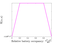
Figure 1: Reward as a function of fractional battery occupancy post current action

Formally, the reward is given by:

$$\begin{split}\mathcal{R}(s,a)=-&\sum_{i=1}^{N}r^{(i)}\Big{\{}(0.2\mathcal{B}^{(i)}-a^{(i)}-b^{(i)})_{+}\\ &\quad+(a^{(i)}+b^{(i)}-0.8\mathcal{B}^{(i)})_{+}\Big{\}},\end{split}$$

where $(z)_{+}:=\max(z,0).$ Note that the reward structure disincentivises operating each battery at close to empty/full charge, the disincentive being (potentially) heterogenous across batteries. (Batteries that suffer a larger degradation due to cycling would be associated with a greater penalty factor $r^{(\cdot)}.$)

Finally, the goal of the learning agent is to maximize the infinite horizon discounted reward, i.e.,

$$\mathbb{E}\left[\sum_{k=0}^{\infty}\gamma^{k}\mathcal{R}(S_{k},A_{k})\right],$$ (5)

for any starting state $S_{0}.$

II-C Policies and Information Structure

In general, a policy specifies the action to be taken as a function of the agent’s observation history. A stationary deterministic policy $\pi\colon\mathcal{S}\rightarrow\mathcal{A}$ specifies a feasible action purely as a function of the current state. It is well known that there exists an optimal stationary deterministic policy that maximizes (5) (see [5]). Moreover, this policy can be computed given the MDP primitives $(\mathcal{S},\mathcal{A},\mathcal{P},\mathcal{R},\gamma)$. In the present context however, it is often impractical to assume prior knowledge of the primitives. In particular, the agent may not a priori know the transition structure $\mathcal{P}$ governing the dynamics of generation/demand evolution precisely. This motivates us to pursue a reinforcement learning (RL) based approach to discover a near-optimal policy online.

For certain special cases (i.e., in the absence of ramp constraints and ignoring losses), it can be proved that a simple greedy policy is in fact optimal for the MDP, as we show in Section III. However, in general, the optimal policy is non-trivial, and we find that the proposed RL based approach (described in Section IV) outperforms naive/greedy policies (see Section V).

III Greedy battery bank management

In this section, we define and explore a greedy policy for the MDP posed in Section II. This policy chooses, in any state, an action that maximizes the instantaneous reward. Importantly, in the context of the battery bank management problem under consideration, this greedy policy can be applied without prior knowledge of the transition structure $\mathcal{P}.$ In other words, the greedy policy can be applied without the need for any ‘learning’ of the MDP dynamics. While the greedy policy is not optimal is general, we show that it is optimal in an idealized special case, namely when the batteries are lossless and are not subject to any ramp constraints. From a practical standpoint, this means that the greedy policy is expected to be near-optimal in scenarios where the batteries are capable of fast charging/discharging, and battery losses are negligible.

Formally, a greedy policy $\pi_{\mathrm{greedy}}$ is defined as follows. In state $s=(x,b),$ it chooses an action

$$\pi_{\mathrm{greedy}}(s)\in\operatorname*{arg\,max}_{a\in\mathcal{A}_{s}}\mathcal{R}(s,a).$$

Note that if there are multiple maximizers of the instantaneous reward, it is assumed that $\pi_{\mathrm{greedy}}$ picks one of them. Note that implementing $\pi_{\mathrm{greedy}}$ requires knowledge of (a) $\mathcal{A}_{s},$ which is dictated by ramp/capacity constraints, and (b) the cycling costs, defined by $(r^{(i)},\ 1\leq i\leq N)$—a reasonable expectation in practice.

The optimality of greedy battery operation in an idealized special case is shown below.

Theorem 1.

For each Battery $i,$ suppose that $c^{(i)}\geq\mathcal{B}^{(i)}$ (i.e., the ramp constraints are never binding), and $\eta^{(i)}=1$ (i.e., the batteries are lossless). Then the policy $\pi_{\mathrm{greedy}}$ is optimal for the infinite horizon discounted reward objective (5).

Proof.

The optimality of any greedy policy follows from two observations. First, in the absence of battery losses, at any time $k,$ the total energy in the battery bank $\sum_{i=1}^{N}B^{(i)}_{k}$ is conserved across all policies. Second, since arbitrary energy rearrangements are possible between batteries (due to the absence of ramp constraints), the instantaneous reward attainable does not depend on the specific placement of energy across batteries. It then follows easily that greedy operation is optimal. ∎

In general, particularly when the battery bank is heterogenous with respect to ramp constraints and/or losses, we find that greedy operation can be far from optimal; see Section V. Intuitively, this is because in such cases, the total energy in the battery bank is not conserved across different policies. Moreover, the presence of ramp constraints implies that there are certain ‘preferrable’ arrangements of the stored energy across the battery bank that minimize average penalties incurred going forward, given the random dynamics of generation/demand. The non-triviality of the optimal policy in the presence of practical constraints on the operation of the battery operation motivates an RL based approach, which we address next.

IV Reinforcement Learning based approach

In this section, we describe an RL based approach for online learning of the optimal policy for battery bank management. Specifically, we employ a $Q$-learning algorithm with linear function approximation [2]. Our key contribution lies in the design of a suitable family kernel functions that captures the specific structure of the value functions in our formulation. The proposed approach is validated via an extensive case study in Section V.

We begin by providing some background on Q-learning. Let us denote an optimal stationary deterministic policy of the MDP by $\pi^{*}$ (the existence of such an optimal policy is guaranteed by the theory; see [5]). The state value function associated with the MDP is defined as

$$V(s):=\mathbb{E}\left[\sum_{k=0}^{\infty}\gamma^{k}\mathcal{R}(S_{k},\pi^{*}(A_{k}))\ |\ S_{0}=s\right].$$

The state-action value function, a.k.a., the $Q$-function associated with the MDP is defined as

$$Q(s,a):=\mathcal{R}(s,a)+\gamma\sum_{s^{\prime}\in\mathcal{S}}\mathcal{P}(s^{\prime}|s,a)V(s^{\prime}).$$

It is well known that the $Q$-function satisfies the Bellman equation:

$$Q(s,a):=\mathcal{R}(s,a)+\gamma\sum_{s^{\prime}\in\mathcal{S}}\mathcal{P}(s^{\prime}|s,a)\left[\max_{a^{\prime}\in\mathcal{A}_{s^{\prime}}}Q(s^{\prime},a^{\prime})\right].$$

Moreover, learning the $Q$-function also reveals the optimal policies, since $\pi^{*}(s)\in\operatorname*{arg\,max}_{a\in\mathcal{A}_{s}}Q(s,a).$

$Q$-learning algorithms seek to learn the $Q$-function online, typically via a stochastic approximation based update rule of the form

$$\hat{Q}(S_{k},A_{k}) \leftarrow\hat{Q}(S_{k},A_{k})+\beta_{k}\biggl{[}\mathcal{R}(S_{k},A_{k})$$

$$\qquad+\gamma\max_{a^{\prime}\in\mathcal{A}_{S_{k+1}}}\hat{Q}(S_{k+1},a^{\prime})-\hat{Q}(S_{k},A_{k})\biggr{]},$$ (6)

where $\beta_{k}\in(0,1)$ is the learning rate (a.k.a., step-size) at time $k.$ Note that the above update rule does not specify the policy that determines the action $A_{k}$ at time $k.$ It is known that (6) results in almost sure convergence to the $Q$-function provided the chosen policy ensures sufficient exploration of all the state-action pairs (see [2]), and the step-size sequence satisfies

$$\sum_{k}\beta_{k}=\infty,\quad\sum_{k}\beta_{k}^{2}<\infty.$$

In the specific application context under consideration, it is not practical to implement $Q$-learning algorithms directly, given the prohibitive number of state-action pairs. This so-called state-action space explosion adversely impacts both the memory footprint of the algorithm (since one must store the entire $Q$-table), and time required to learn a near-optimal policy (since each state-action pair needs to be visited sufficiently many times). We thus resort to function approximation, wherein the $Q$-function is approximated to be a linear combination of carefully designed family of features or kernel functions:

$$Q(s,a,w)\approx\phi(s,a)^{T}\cdot w=\sum_{i=1}^{d}\phi_{i}(\cdot)w_{i}$$ (7)

Here, $\phi(s,a)\in\mathbb{R}^{d}$ is a vector consisting of $d$ distinct features corresponding to state-action pair $(s,a)$ and $w\in\mathbb{R}^{d}$ is the weight vector to be learned. Naturally, this is appealing when $d\ll|\{(s,a)|s\in\mathcal{S},a\in\mathcal{A}_{s}\}|.$

In the remainder of this section, we describe our design of the family of features, and then state formally the proposed RL algorithm.

IV-A Design of Kernel functions

The $d$ distinct features chosen for each state-action pair $(s,a),$ where $s=(x,b),$ are captured in the feature vector $\phi(\cdot)$ as follows

$$\phi(s,a)=\big{(}\mathcal{R}(s,a),\ v_{1}\mathds{1}_{\{x=1\}}, \ v_{2}\mathds{1}_{\{x=2\}},$$

$$\cdots,v_{|S_{e}|}\mathds{1}_{\{x=|S_{e}|\}}\big{)}.$$

Here each vector $v_{j}\in\mathbb{R}^{2N}$ corresponds to the $j^{th}$ state of the background DTMC $\{X_{k}\}$ governing the net generation, and is defined as $v_{j}=$

$$\Big{(}1,-(1-y_{1})^{4},-y_{1}^{4},-(1-y_{2})^{4},-y_{2}^{4},\cdots,-(1-y_{N})^{4},-y_{N}^{4}\Big{)}$$ (8)

where $y_{i}$ denotes the normalised occupancy of Battery $i,$ given by $y_{i}=\frac{b^{(i)}+a^{(i)}}{\mathcal{B}^{(i)}}.$ Thus, in our design, $d=(2N+1)|\mathcal{S}|+1.$

The first feature is simply the instantaneous reward corresponding to the state action pair $(s,a).$ The remaining features are interpreted as follows. For each background state $x,$ and for each Battery $i,$ we introduce two features: an increasing concave function of the normalized battery occupancy resulting from the action $a,$ and another descreasing concave function of the same normalized battery occupancy; see Figure 2.

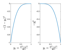
Figure 2: Two Kernel functions as a function of normalised battery level $y_{i}.$

The former captures the impending (discounted) penalty arising from Battery $i$ becoming empty in the future; the increasing shape of this function seeks to capture the increased likelihood of a penalty in the near future when the present battery occupancy is lower (see the left panel of Figure 2). Similarly, the latter feature captures the discounted ‘penalty to go’ arising due to Battery $i$ becoming full in the future; the descreasing nature of this function capturing the increased likelihood of this event when the present battery occupancy is closer to full (see the right panel of Figure 2). We introduce these two features for each background state $x$ separately to account for the fact that the probability of future penalties is also dictated by $x.$ In addition, for each background state $x,$ we add a constant feature taking the value 1 (see equation (8)). As we show in Section V, this family of features captures the behavior of the $Q$-function sufficiently well to enable the learning of a near-optimal policy.

IV-B Learning weights via stochastic semi-gradient descent

The weight vector $w$ in (7) is learned online by stochastic semi-gradient descent method using a suffiently exploratory policy $\pi$ over state-action pair $(s,a).$ The term ‘semi’ refers to the fact that the error being minimized through gradient descent is between the estimated values $\hat{Q}(S_{k},A_{k},w_{k})$ and $\left(R(S_{k},A_{k})+\gamma\max_{a^{\prime}\in\mathcal{A}_{S_{k+1}}}\hat{Q}(S_{k+1},a^{\prime},w_{k})\right).$ The update of weights is performed in conjunction with an $\epsilon$-greedy policy to ensure a balance between exploration and exploitation.

Formally, the weights are updated using stochastic semi-gradient descent as follows:

$$w \leftarrow w+\beta_{k}\big{[}\mathcal{R}(S_{k},A_{k})+\gamma\max_{a\in\mathcal{A}_{S_{k+1}}}\hat{Q}(S_{k+1},a,w)$$

$$\quad-\hat{Q}(S_{k},A_{k},w)\big{]}\phi(S_{k},A_{k}),$$ (9)

where $\hat{Q}(s,a,w)=\phi(s,a)^{T}w.$ Here, $\{\beta_{k}\}$ is the step-size sequence. The policy $\pi$ that selects the action $A_{k}$ at each time $k$ is taken to be the $\epsilon$-greedy policy, parameterized by the sequence $\{\epsilon_{k}\}.$ Formally, at time $k,$ with probability $\epsilon_{k},$ the action $A_{k}$ is picked uniformly at randomly from the set $\mathcal{A}_{S_{k}},$ and with probabability $1-\epsilon_{k},$ $A_{k}=\operatorname*{arg\,max}_{a\in\mathcal{A}_{S_{k}}}Q(S_{k},a).$

V Case Study

In this section, we present simulation results on a toy model to validate the proposed function approximation based RL algorithm. We benchmark the performance of this policy against a certain naive policy (which charges and discharges the battery bank in a proportional manner) as well as a greedy policy. Our results demonstrate that the proposed approach outperforms the greedy and naive policies, suggesting that the proposed collection of features does a good job of capturing the structure of the value function.

To provide a fair comparison between the three policies, we separate the learning and the evaluation phases of our proposed policy. Specifically, we learn the $Q$-table via function approximation using the proposed algorithm over $T=10^{5}$ time steps. After this, we compare the ‘optimal’ policy suggested by the learned $Q$-function, i.e.,

$$\pi_{\mathrm{RL(fun\ approx)}}(s)\in\operatorname*{arg\,max}_{a\in\mathcal{A}_{s}}\hat{Q}(s,a,w),$$ (10)

against the benchmark policies over another run of $T$ time steps.

While the greedy policy has been described in Section III, the naive (proportional) policy is described as follows. In essence, it attempts to apportion the net generation across the battery bank in a manner that is proportional to the size of each battery, i.e., $a^{(i)}\propto\mathcal{B}^{(i)}.$ Of course, a perfectly proportional allocation may not be feasble, due to interger-round off errors, as well as ramp constraints. If this happens, the naive policy performs a local search around the proportional allocation until a feasible action is found; the details of this search are omitted due to space constraints.

Toy Model Setup

The state space of the background DTMC process $X_{k}$ is taken to be $\mathcal{S}_{e}=\{-4,-1,1,5\},$ with the net generation associated with state $x\in\mathcal{S}_{e}$ being simply $x.$ The transition probability matrix corresponding to the background Markov process $\{X_{k}\}$ is taken to be

$$P=\begin{bmatrix}0&0.5&0.3&0.2\\ 0.5&0&0.1&0.4\\ 0.3&0.2&0&0.5\\ 0.3&0.3&0.4&0\end{bmatrix}.$$

Two battery units are considered with penalty multipliers $r^{(1)}=-0.1,\ r^{(2)}=-1;$ this captures the heterogeneity in cycling costs. Various battery size configurations $(\mathcal{B}^{(1)},\mathcal{B}^{(2)})$ are considered for the simulation; see Tables I-II. For simplicity, we ignore losses in these preliminary evaluations.

Simulation results

First, we consider the case where ramp constraints are never binding (by choosing $(c^{(i)},\ 1\leq i\leq N)$ large enough). In this case, it is known that greedy operation is optimal, allowing us to evaluate whether or not the proposed function approximation based approach is also able to learn the optimal policy. Our results, comparing the rewards obtained by the three policies under consideration, are summarized in Table I. Interestingly, we see in that all settings considered, the proposed RL based approach achieves exactly the same reward as the (optimal) greedy policy, whereas the naive policy performs worse. This suggests that for the MDP instances considered here, the proposed function approximation algorithm learns an optimal policy, validating our design of the kernel functions.

Next, we consider settings where ramp constraints can be binding. Specifically, we set $c^{(1)}=c^{(2)}=2.$ The results for case, corresponding to various battery size combinations, are summarized in Table II. Note that the proposed RL based approach outperforms both the (no longer optimal) greedy policy, as well as the naive policy.

Validating the proposed approach on ‘production scale’ MDP instances, derived from real-world generation/demand traces, will be the addressed in a forthcoming journal version of this paper.

$(\mathcal{B}^{(1)},\mathcal{B}^{(2)})$	$\pi_{\text{greedy}}$	$\pi_{\text{naive}}$	$\pi_{\text{RL(function approx.)}}$
2,3	-68081	-68081	-68081
3,5	-48532	-51187	-48532
6,10	-63853	-73619	-63853
10,10	-57859	-74729	-57859
15,10	-52768	-74842	-52768
15,15	-72490	-110960	-72490
20,20	-91273	-144160	-91273

TABLE I: Reward obtained across different policies when no constraints are imposed: $S_{e}=\{-4,-1,1,5\},$ $T=10^{5};$ cycling costs prefactors $r^{(1)}=-0.1,r^{(2)}=-1$

$(\mathcal{B}^{(1)},\mathcal{B}^{(2)})$	$\pi_{\text{greedy}}$	$\pi_{\text{naive}}$	$\pi_{\text{RL(function approx.)}}$
2,3	-61212	-61212	-61212
3,5	-45010	-46861	-44831
6,10	-60759	-64053	-61774
10,10	-66177	-67867	-56920
15,10	-66146	-67849	-54579
15,15	-80171	-96938	-68135
20,20	-88881	-115150	-75473
25,25	-99762	-147800	-87300
30,30	-119320	-184450	-105630
40,40	-125130	-230460	-113120
50,50	-137580	-286050	-125350

TABLE II: Reward obtained across different policies when constraints are imposed: $c^{(1)}=c^{(2)}=2,$ $S_{e}=\{-4,-1,1,5\},$ $T=10^{5};$ cycling costs prefactors $r^{(1)}=-0.1,r^{(2)}=-1$

VI Related literature and concluding remarks

In this section, we briefly survey some of the related literature, and then conclude.

There are a few approaches in the literature for operating multiple heterogeneous battery units. The work in [6] proposes a feedback control mechanism to maintain uniform state-of-charge (SOC) across multiple batteries without considering the cycling cost. The work [7] proposes another feedback mechanism to control power flow in storage systems. A circuit based switching mechanism to operate serially connected battery units is studied in [8]. A coordinated control of multiple battery systems for frequency regulation is given in [9], which also proposes a state-of-charge (SOC) recovery mechanism. These are non-RL approaches which deal with battery bank operation with specific operational objectives in mind. The supply-side uncertainty due to renewables, which is central to the management of grid-scale storage solutions, is not considered in these works.

On the RL front, the work in [10] proposes an energy management system using deep reinforcement learning to operate the battery pack in an electric vechicle.

In contrast, the focus of the present paper is on the management of a heterogenous bank of batteries connected to the grid, with the objective of minimizing the cycling-induced degradation of the bank. The key novelty of the approach proposed in this paper is the use of linear function approximation to address the state-action space explosion that occurs due to (i) the incorporation of the battery levels into the state, and (ii) the combinatorial number of actions that are feasible for each state. We design a novel and compact collection of feature vectors that let us approximate the structure of the $Q$-function, enabling the learning of a near-optimal policy online.

Future work will focus on validating the proposed approach on a practical utility-scale example, with cycling costs and losses modeled using manufacturer-provided specifications. In such a case, one would expect the net generation process to be made up of components that fluctuate over multiple timescales, resulting in a highly non-trivial optimal operation of the battery bank.

References

- Cole and Frazier [2019] W. J. Cole and A. Frazier, “Cost projections for utility-scale battery storage,” National Renewable Energy Laboratory (NREL), Tech. Rep., 2019.
- Sutton and Barto [2018] R. S. Sutton and A. G. Barto, Reinforcement learning: An introduction. MIT press, 2018.
- Kazhamiaka et al. [2018] F. Kazhamiaka, S. Keshav, C. Rosenberg, and K.-H. Pettinger, “Simple spec-based modeling of lithium-ion batteries,” IEEE Transactions on Energy Conversion, vol. 33, no. 4, pp. 1757–1765, 2018.
- Garche et al. [1997] J. Garche, A. Jossen, and H. Döring, “The influence of different operating conditions, especially over-discharge, on the lifetime and performance of lead/acid batteries for photovoltaic systems,” Journal of Power Sources, vol. 67, no. 1-2, pp. 201–212, 1997.
- Puterman [2014] M. L. Puterman, Markov decision processes: discrete stochastic dynamic programming. John Wiley & Sons, 2014.
- Wang et al. [2015] C. Wang, G. Yin, F. Lin, M. P. Polis, C. Zhang, J. Jiang et al., “Balanced control strategies for interconnected heterogeneous battery systems,” IEEE Transactions on Sustainable Energy, vol. 7, no. 1, pp. 189–199, 2015.
- Bauer et al. [2019] M. Bauer, M. Mühlbauer, O. Bohlen, M. A. Danzer, and J. Lygeros, “Power flow in heterogeneous battery systems,” Journal of Energy Storage, vol. 25, 2019.
- Shibata et al. [2001] H. Shibata, S. Taniguchi, K. Adachi, K. Yamasaki, G. Ariyoshi, K. Kawata, K. Nishijima, and K. Harada, “Management of serially-connected battery system using multiple switches,” in IEEE PEDS 2001, vol. 2, 2001.
- Zhu and Zhang [2018] D. Zhu and Y.-J. A. Zhang, “Optimal coordinated control of multiple battery energy storage systems for primary frequency regulation,” IEEE Transactions on Power Systems, vol. 34, no. 1, pp. 555–565, 2018.
- Chaoui et al. [2018] H. Chaoui, H. Gualous, L. Boulon, and S. Kelouwani, “Deep reinforcement learning energy management system for multiple battery based electric vehicles,” in IEEE Vehicle Power and Propulsion Conference (VPPC), 2018.