Light baryonium spectrum

Abstract

We evaluate the light baryonium spectrum, viz. the baryon-antibaryon states, in the framework of QCD sum rules. The nonperturbative contributions up to dimension 12 are taken into account. Numerical results indicate that there might exist eight possible light baryonium states, i.e. $p$-$\bar{p}$, $\Lambda$-$\bar{\Lambda}$, $\Sigma$-$\bar{\Sigma}$, and $\Xi$-$\bar{\Xi}$ with quantum numbers of $0^{-+}$ and $1^{--}$. For the $\Lambda$-$\bar{\Lambda}$, $\Sigma$-$\bar{\Sigma}$, and $\Xi$-$\bar{\Xi}$ states, their masses are found above the corresponding dibaryon thresholds, while the masses of $p$-$\bar{p}$ states are not. The possible baryonium decay modes are analyzed, which are hopefully measurable in BESIII, BELLEII, and LHCb experiments.

I Introduction

The establishment of quark model (QM) in 1960s GellMann:1964nj ; Zweig led to a renaissance in the exploration of micro worlds. The spectroscopy of conventional hadrons ($q\bar{q}$ or $qqq$) in QM is being gradually confirmed through experiments and will be completed soon. Entering the new millennium, with development of technology, the emergence of the so-called exotic state such as X(3872) has been reported Choi:2003ue , and new ones tend to appear more frequently. Presently, a bunch of charmoniumlike/bottomoniumlike states XYZ and pentaquark states $P_{c}$ are observed in experiments; this situation is similar to the phase of “particle zoo” witnessed in the last century. To discover more exotic states and explore their properties is currently one of the most intriguing and important topics in particle physics, which may greatly enrich the hadron family and our knowledge of the nature of QCD.

Facing the observations of tetraquark and pentaquark states, it is nature to conjecture existence of the hexaquark states, and it is time for hunting them. Deuteron, created at the beginning of the Universe and its stability is responsible for the production of other elements, is a typical and well-established dibaryon molecular state with $J^{P}=1^{+}$ and binding energy $E_{B}=2.225\text{MeV}$ Weinberg:1962hj . Interestingly, the strong interactions bring stability to deuterons and also allow various other stable deuteronlike dibaryon states; however, no such states, though speculated about many times Jaffe:1976yi ; Mulders:1980vx ; Balachandran:1983dj ; Sakai:1999qm ; Ikeda:2007nz ; Bashkanov:2013cla ; Shanahan:2011su ; Clement:2016vnl , have been observed yet BaBar:2018hpv . On the other hand, the baryonium state composed of a baryon-antibaryon pair is another special class of heaxquark configuration. The interaction between baryon-antibaryon pair is analogous to that between two baryons, which will provide important hints to understanding the absence in observation of the stable deuteronlike dibaryon states.

Actually, the history of the investigation of baryon-antibaryon states dates back to the 1940s, when Fermi and Yang proposed that $\pi$-mesons may be composite particles formed by the association of a nucleon with an antinucleon Fermi:1949voc , and their scenario was later on replaced by the quark model. Entering the new millennium, the heavy baryon-antibaryon hadronic structures, and, hence, the term of baryonium, were proposed and employed to explain the extraordinary nature of $Y(4260)$ Qiao:2005av ; Qiao:2007ce and other charmoniumlike states observed in experiments. Later on, more investigations on baryonium are performed from various aspects Chen:2011cta ; Chen:2013sba ; Wan:2019ake ; Chen:2016ymy ; Liu:2007tj ; Wang:2021qmn . Partly due to the the small spacings between light hadron states, it is normally hard to discriminate exotic states from conventional ones. However, with a large amount of $J/\psi$ samples, BESIII Collaboration is carefully examining the physics happening in the energy region around $2.0$ GeV BESIII:2010gmv ; BES:2003aic ; BES:2005ega ; BESIII:2010vwa ; BESIII:2019wkp ; BESIII:2016qzq ; BESIII:2020vtu ; BESIII:2017kqw ; BESIII:2017hyw ; BESIII:2019cuv , which motivates a fresh interest in light exotic states . In the literature, theoretical investigations on light baryonium were made through various techniques, including flux tube model Deng:2012wi ; Deng:2013aca , one-boson-exchange potential (OBEP) model Zhao:2013ffn , Bethe-Salpeter approach Zhu:2019ibc ; Wang:2010vz , and QCD sum rules (QCDSR) Wang:2006sna .

Of those techniques, the model with the independent Shifman, Vainshtein, and Zakharov (SVZ) sum rule technique Shifman has some peculiar advantages in exploring hadron properties involving nonperturbative QCD. Rather than a phenomenological model, QCDSR is a QCD based theoretical framework which incorporates nonperturbative effects universally order by order and has already achieved a lot in the study of hadron spectroscopy and decays. Its starting point is to construct the proper interpolating currents corresponding to the hadron of interest ,which possesses the foremost information about the concerned hadron, like quantum numbers and the constituent quark or gluon. With the currents, the two-point correlation function, which has two representations, the QCD representation and the phenomenological representation, can be constructed. Equating these two representations, the QCD sum rules will be formally established, from which the hadron mass and decay width may be deduced.

In this work, we investigate the light baryonium states, i.e., $\mathscr{B}$-$\bar{\mathscr{B}}$ states with quantum numbers $J^{PC}=0^{++}$, $0^{-+}$, $1^{++}$ and $1^{--}$ in the framework of QCD sum rules, where $\mathscr{B}$ denotes light baryon. The possible baryonium decay channels are also analyzed. The rest of the paper is organized as follows. After the introduction, a brief interpretation of QCD sum rules and some primary formulas in our calculation are presented in Sec. II. We give the numerical analysis and results in Sec. III. In Sec. IV, possible decay modes of light baryonium states are investigated. The last part is left for conclusions and discussions.

II Formalism

To evaluate the mass spectrum of $\mathscr{B}$-$\bar{\mathscr{B}}$ states in QCDSR, the appropriate currents coupling to the states have to be constructed. The lowest order interpolating currents for $\mathscr{B}$-$\bar{\mathscr{B}}$ states with quantum numbers $0^{++}$, $0^{-+}$, $1^{++}$, and $1^{--}$ can be respectively constructed as

$$j^{0^{-+}}(x) = i\,\bar{\eta}_{\mathscr{B}}(x)\gamma_{5}\eta_{\mathscr{B}}(x)\;,$$ (1)

$$j^{1^{--}}_{\mu}(x) = \bar{\eta}_{\mathscr{B}}(x)\gamma_{\mu}\eta_{\mathscr{B}}(x)\;,$$ (2)

$$j^{0^{++}}(x) = \bar{\eta}_{\mathscr{B}}(x)\eta_{\mathscr{B}}(x)\;,$$ (3)

$$j^{1^{++}}_{\mu}(x) = i\,\bar{\eta}_{\mathscr{B}}(x)\gamma_{\mu}\gamma_{5}\eta_{\mathscr{B}}(x)\;.$$ (4)

Here, we use the notion $\eta_{\mathscr{B}}$ to represent the Dirac baryon fields without free Lorentz indices. As shown in Ref. Chung:1981wm , $\eta_{\mathscr{B}}$ may takes the following quark structure :

$$\eta_{\mathscr{B}}(x) = i\epsilon_{abc}[q_{a}^{i\,T}(x)C\gamma_{5}q_{b}^{j}(x)]q^{k}_{c}(x)\;,$$ (5)

where the superscripts $i$, $j$, and $k$ denote the flavor of light quarks, subscripts $a$, $b$, and $c$ are color indices, and $C$ is the charge conjugation matrix. In our calculation, $(i,j,k)=(u,d,u)$, $(u,d,s)$, $(u,s,d)$, and (s, u, s) for $p$, $\Lambda$, $\Sigma$ and $\Xi$ states, respectively.

With the currents (1)$-$(4), the two-point correlation function can be readily established, i.e.,

$$\Pi(q^{2}) = i\int d^{4}xe^{iq\cdot x}\langle 0|T\{j(x),\;j^{\dagger}(0)\}|0\rangle\;,$$ (6)

$$\Pi_{\mu\nu}(q^{2}) = i\int d^{4}xe^{iq\cdot x}\langle 0|T\{j_{\mu}(x),\;j_{\nu}^{\dagger}(0)\}|0\rangle\;$$ (7)

where $j(x)$ and $j_{\mu}(x)$ are the relevant hadronic currents with $J=0$ and 1, respectively, and $|0\rangle$ denotes the physical vacuum. For $j_{\mu}(x)$, the correlation function has the following Lorentz covariance form:

$$\Pi_{\mu\nu}(q^{2}) = -\Big{(}g_{\mu\nu}-\frac{q_{\mu}q_{\nu}}{q^{2}}\Big{)}\Pi_{1}(q^{2})+\frac{q_{\mu}q_{\nu}}{q^{2}}\Pi_{0}(q^{2})\;,$$ (8)

where the subscripts $1$ and $0$, respectively, denote the quantum numbers of the spin 1 and 0 mesons.

On the phenomenological side, after separating the ground state contribution from the hadronic state, the correlation function $\Pi^{X}_{J^{PC}}(q^{2})$ can be expressed as a dispersion integral over the physical regime, i.e.,

$$\Pi^{X,\;phen}_{J^{PC}}(q^{2}) = \frac{(\lambda^{X}_{J^{PC}})^{2}}{(m^{X}_{J^{PC}})^{2}-q^{2}}+\frac{1}{\pi}\int_{s_{0}}^{\infty}ds\frac{\rho^{X}_{J^{PC}}(s)}{s-q^{2}}\;,$$ (9)

where the superscript $X$ denotes the lowest lying $\mathscr{B}$-$\bar{\mathscr{B}}$ hexaquark state, $m^{X}_{J^{PC}}$ is the mass of $X$ with the quantum number of $J^{PC}$, $\rho^{X}_{J^{PC}}(s)$ is the spectral density that contains the contributions from higher excited states and the continuum states above the threshold $s_{0}$, and $\lambda^{X}$ is the coupling constant.

On the OPE (operator product expansion) side, the dispersion relation can express the correlation function $\Pi^{X}_{J^{PC}}(q^{2})$ as

$$\Pi^{X,\;OPE}_{J^{PC}}(q^{2}) = \int_{s_{min}}^{\infty}ds\frac{\rho^{X,\;OPE}_{J^{PC}}(s)}{s-q^{2}}\;,$$ (10)

where $s_{min}$ is the kinematic limit, which usually corresponds to the square of the sum of current-quark masses of the hadron Wan:2020oxt ; Wan:2020fsk . $\rho^{X,\;OPE}_{J^{PC}}(s)=\text{Im}[\Pi^{X,\;OPE}_{J^{PC}}(s)]/\pi$ is the spectral density of the OPE side and contains the contributions of the condensates up to dimension 12 which can be expressed as:

$$\rho^{OPE}(s) = \rho^{pert}(s)+\rho^{\langle\bar{q}q\rangle}(s)+\rho^{\langle G^{2}\rangle}(s)+\rho^{\langle\bar{q}Gq\rangle}(s)+\rho^{\langle\bar{q}q\rangle^{2}}(s)+\rho^{\langle G^{3}\rangle}(s)$$ (11)

$$+ \rho^{\langle\bar{q}q\rangle\langle\bar{q}Gq\rangle}(s)+\rho^{\langle\bar{q}q\rangle^{2}\langle G^{2}\rangle}(s)+\rho^{\langle\bar{q}Gq\rangle^{2}}(s)+\rho^{\langle\bar{q}q\rangle^{2}\langle\bar{q}Gq\rangle}(s)+\rho^{\langle\bar{q}q\rangle^{4}}(s)$$

$$= \sum_{n}c_{n}s^{n}.$$

Here, $c_{n}$ is the coefficient of the $s^{n}$ term with corresponding vacuum condensates.

To calculate the spectral density of the OPE side, Eq. (11), the full propagators $iS^{q}_{ij}(x)$ of a light quark ($q=u$, $d$, or $s$) are used:

$$iS^{q}_{jk}(x)\!\! = \!\!\frac{i\delta_{jk}x\!\!\!/}{2\pi^{2}x^{4}}-\frac{\delta_{jk}m_{q}}{4\pi^{2}x^{2}}-\frac{it^{a}_{jk}G^{a}_{\alpha\beta}}{32\pi^{2}x^{2}}(\sigma^{\alpha\beta}x\!\!\!/+x\!\!\!/\sigma^{\alpha\beta})-\frac{\delta_{jk}}{12}\langle\bar{q}q\rangle+\frac{i\delta_{jk}x\!\!\!/}{48}m_{q}\langle\bar{q}q\rangle-\frac{\delta_{jk}x^{2}}{192}\langle g_{s}\bar{q}\sigma\cdot Gq\rangle$$ (12)

$$+ \frac{i\delta_{jk}x^{2}x\!\!\!/}{1152}m_{q}\langle g_{s}\bar{q}\sigma\cdot Gq\rangle-\frac{t^{a}_{jk}\sigma_{\alpha\beta}}{192}\langle g_{s}\bar{q}\sigma\cdot Gq\rangle+\frac{it^{a}_{jk}}{768}(\sigma_{\alpha\beta}x\!\!\!/+x\!\!\!/\sigma_{\alpha\beta})m_{q}\langle g_{s}\bar{q}\sigma\cdot Gq\rangle\;,$$

where, the vacuum condensates are clearly displayed. For more explanation on above propagator, readers may refer to Refs. Wang:2013vex ; Albuquerque:2013ija .

Performing a Borel transform on both Eq. (9) and Eq. (10), and matching the OPE side with the phenomenological side of the correlation function $\Pi(q^{2})$, one can finally obtain the mass of the hexaquark state,

$$m^{X}_{J^{PC}}(s_{0},M_{B}^{2})=\sqrt{-\frac{L^{X}_{J^{PC},\;1}(s_{0},M_{B}^{2})}{L^{X}_{J^{PC},\;0}(s_{0},M_{B}^{2})}}\;.$$ (13)

Here $L_{0}$ and $L_{1}$ are respectively defined as

$$L^{X}_{J^{PC},\;0}(s_{0},M_{B}^{2})=\int_{s_{min}}^{s_{0}}ds\;\rho^{X,\;OPE}_{J^{PC}}(s)e^{-s/M_{B}^{2}}\;$$ (14)

and

$$L^{X}_{J^{PC},\;1}(s_{0},M_{B}^{2})=\frac{\partial}{\partial{\frac{1}{M_{B}^{2}}}}{L^{X}_{J^{PC},\;0}(s_{0},M_{B}^{2})}\;.$$ (15)

III Numerical analysis

In the numerical calculation of QCD sum rules, the input parameters are taken from Albuquerque:2013ija ; Matheus:2006xi ; Cui:2011fj ; Narison:2002pw ; P.Col ; Tang:2019nwv ; pdg :

$$\begin{aligned} &\langle\bar{q}q\rangle=-(0.24\pm 0.01)^{3}\;\text{GeV}^{3}\;,&&\langle\bar{s}s\rangle=(1.15\pm 0.12)\langle\bar{q}q\rangle\;,\\ &\langle g_{s}^{2}G^{2}\rangle=(0.88\pm 0.25)\;\text{GeV}^{4}\;,&&\langle g_{s}^{3}G^{3}\rangle=(0.045\pm 0.013)\;\text{GeV}^{6}\;,\\ &\langle\bar{q}g_{s}\sigma\cdot Gq\rangle=m_{0}^{2}\langle\bar{q}q\rangle\;,&&\langle\bar{s}g_{s}\sigma\cdot Gs\rangle=m_{0}^{2}\langle\bar{s}s\rangle\;,\\ &m_{0}^{2}=(0.8\pm 0.1)\;\text{GeV}^{2}\;,&&m_{s}=(95\pm 5)\;\text{MeV}\;,\\ &m_{u}=2.16^{+0.49}_{-0.26}\;\text{MeV}\;,&&m_{d}=4.67^{+0.48}_{-0.17}\;\text{MeV}\;,\end{aligned}$$ (16)

Note, a large strange quark condensate value is taken in numerical evaluation according to the recent lattice QCD calculation Davies:2018hmw .

Furthermore, there exist two additional parameters, i.e., the continuum threshold $s_{0}$ and the Borel parameter $M_{B}^{2}$, introduced in establishing the sum rule, which can be fixed in light of the so-called standard procedures abiding by two criteria Shifman ; Reinders:1984sr ; P.Col . The first one asks for the convergence of the OPE, which is to compare individual contributions with the overall magnitude on the OPE side, and then a reliable region for $M_{B}^{2}$ will be chosen to retain the convergence. The second criterion of QCD sum rules is the pole contribution (PC). As discussed in Refs. Chen:2014vha ; Azizi:2019xla ; Wang:2017sto , the large power of $s$ in the spectral density suppresses the PC value; thus, the pole contribution will be chosen larger than $15\%$ for hexaquark states. The two criteria can be formulated as follows:

$$R^{X,\;OPE}_{J^{PC}}=\left|\frac{L_{J^{PC},\;0}^{X,\;c_{0}}(s_{0},M_{B}^{2})}{L_{J^{PC},\;0}^{X}(s_{0},M_{B}^{2})}\right|\,,$$ (17)

$$R^{X,\;PC}_{J^{PC}}=\frac{L_{J^{PC},\;0}^{X}(s_{0},M_{B}^{2})}{L_{J^{PC},\;0}^{X}(\infty,M_{B}^{2})}\;.$$ (18)

Here, the superscript $c_{0}$ denotes the contribution given by the $c_{0}$ term. In addition, to find an optimal Borel window the contributions of $c_{1}$, $c_{2}$, and $c_{3}$ terms are also taken into account.

In order to determine a proper value for $s_{0}$, a similar analysis in Refs. Qiao:2013dda ; Tang:2016pcf ; Wan:2020oxt ; Wan:2020fsk will be carried out. Since the continuum threshold $s_{0}$ relates to the mass of the ground state by $\sqrt{s_{0}}\sim(m^{X}+\delta)$, in which $\delta$ lies in the range $0.4-0.8$ GeV P.Col ; Finazzo:2011he , various $\sqrt{s_{0}}$ satisfying this constraint are taken into account. Among these values, the one which yields an optimal window for Borel parameter $M_{B}^{2}$ should be selected out. That is, within the optimal window, the mass of hexaquark is somehow independent of the Borel parameter $M_{B}^{2}$ as much as possible. In practice, we will vary $\sqrt{s_{0}}$ by $0.1$ GeV, which obtained the lower and upper bounds hence the uncertainties of $\sqrt{s_{0}}$.

With the above preparation the mass spectrum of baryonium in light sector will be numerically evaluated. For $p$-$\bar{p}$ states, the ratios $R^{N\bar{N},\;OPE}_{0^{-+}}$ and $R^{N\bar{N},\;PC}_{0^{-+}}$ are shown as functions of Borel parameter $M_{B}^{2}$ in Fig. 1(a) and Fig. 1(b) with different values of $\sqrt{s_{0}}$, i.e., $2.4$, $2.5$, and $2.6$ GeV. Since the $c_{0}$ term will vanish in the chiral limit, we estimate the OPE convergence by inspecting the contributions of $c_{1}$ over $c_{2}$ and $c_{2}$ over $c_{3}$, which clearly indicate that higher dimensional terms yield relative small contributions, as shown in Figs. 1$-$4. The dependence relationships between $m^{N\bar{N}}_{0^{-+}}$ and parameter $M_{B}^{2}$ are given in Fig. 1(c). The optimal Borel window is found in the range $1.6\leq M_{B}^{2}\leq 2.2\;\text{GeV}^{2}$, and the mass $m^{N\bar{N}}_{0^{-+}}$ can be extracted as follows:

$$m^{N\bar{N}}_{0^{-+}} = (1.81\pm 0.09)\;\text{GeV}.$$ (19)

The ratios $R^{N\bar{N},\;OPE}_{1^{--}}$ and $R^{N\bar{N},\;PC}_{1^{--}}$ are presented in Fig. 1(d) and Fig. 1(e) with different values of $\sqrt{s_{0}}$, i.e., $2.4$, $2.5$, and $2.6$ GeV, and the relationships between $m^{N\bar{N}}_{1^{--}}$ and parameter $M_{B}^{2}$ are displayed in Fig. 1(f). The optimal Borel window is found in $1.6\leq M_{B}^{2}\leq 2.2\;\text{GeV}^{2}$, and the mass $m^{N\bar{N}}_{1^{--}}$ can be evaluated as follows:

$$m^{N\bar{N}}_{1^{--}} = (1.82\pm 0.10)\;\text{GeV}.$$ (20)

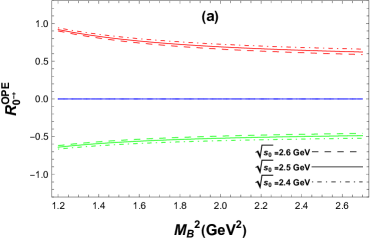
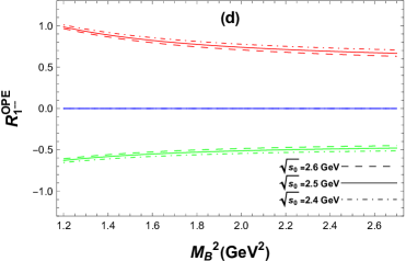
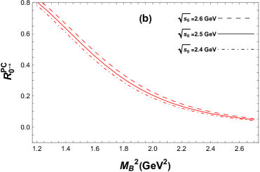
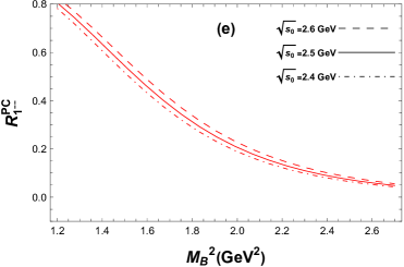
Figure 1: Figures for $N$-$\bar{N}$ baryonium states. (a) The ratio ${R_{0^{-+}}^{OPE}}$ state as functions of the Borel parameter $M_{B}^{2}$ for different values of $\sqrt{s_{0}}$, where blue lines, red lines, and green lines represent the contribution of $c_{0}$ terms, contributions of $c_{1}$ over $c_{2}$, and the contribution of $c_{2}$ over $c_{3}$, respectively. (b) The pole contribution ${R_{0^{-+}}^{PC}}$ as functions of the Borel parameter $M_{B}^{2}$ for different values of $\sqrt{s_{0}}$. (c) The mass $M_{0^{-+}}^{N\bar{N}}$ as a function of the Borel parameter $M_{B}^{2}$ for different values of $\sqrt{s_{0}}$. The same captions for (d), (e) and (f) as in (a), (b) and (c), respectively, but for the $1^{--}$ state.

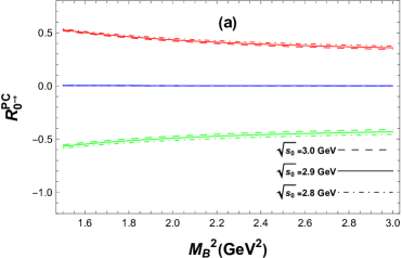
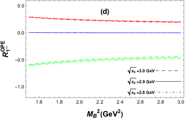
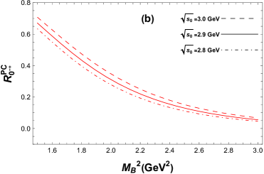
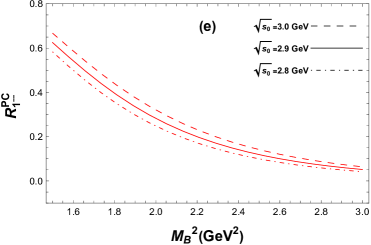
Figure 2: The same caption as in Fig. 1, but for the $\Lambda$-$\bar{\Lambda}$ states.

For $\Lambda$-$\bar{\Lambda}$ states, we show the ratios $R^{\Lambda\bar{\Lambda},\;OPE}_{0^{-+}}$ and $R^{\Lambda\bar{\Lambda},\;PC}_{0^{-+}}$ in Fig. 2(a) and Fig. 2(b) with different values of $\sqrt{s_{0}}$, i.e., $2.8$, $2.9$, and $3.0$ GeV, and the relationships between $m^{\Lambda\bar{\Lambda}}_{0^{-+}}$ and parameter $M_{B}^{2}$ are given in Fig. 2(c). The optimal Borel window is found in $1.9\leq M_{B}^{2}\leq 2.5\;\text{GeV}^{2}$, and the mass $m^{\Lambda\bar{\Lambda}}_{0^{-+}}$ can be obtained as follows:

$$m^{\Lambda\bar{\Lambda}}_{0^{-+}} = (2.27\pm 0.13)\;\text{GeV}.$$ (21)

The ratios $R^{\Lambda\bar{\Lambda},\;OPE}_{1^{--}}$ and $R^{\Lambda\bar{\Lambda},\;PC}_{1^{--}}$ are shown in Fig. 2(d) and Fig. 2(e), where $\sqrt{s_{0}}=2.8$, $2.9$, and $3.0$ GeV, respectively, and we display the relationships between $m^{\Lambda\bar{\Lambda}}_{1^{--}}$ and parameter $M_{B}^{2}$ in Fig. 2(f). The optimal Borel window is found in $1.9\leq M_{B}^{2}\leq 2.5\;\text{GeV}^{2}$, and the mass $m^{\Lambda\bar{\Lambda}}_{1^{--}}$ can be estimated as follows:

$$m^{\Lambda\bar{\Lambda}}_{1^{--}} = (2.34\pm 0.12)\;\text{GeV}.$$ (22)

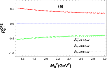
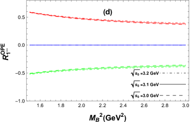
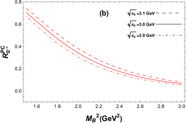
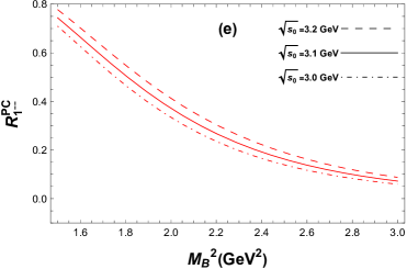
Figure 3: The same caption as in Fig. 1, but for the $\Sigma$-$\bar{\Sigma}$ states.

For the $\Sigma$-$\bar{\Sigma}$ states, the ratios $R^{\Sigma\bar{\Sigma},\;OPE}_{0^{-+}}$ and $R^{\Sigma\bar{\Sigma},\;PC}_{0^{-+}}$ can be found in Fig. 3(a) and Fig. 3(b) with different values of $\sqrt{s_{0}}$, i.e., $2.9$, $3.0$, and $3.1$ GeV, and the relationships between $m^{\Sigma\bar{\Sigma}}_{0^{-+}}$ and parameter $M_{B}^{2}$ are presented in Fig. 3(c). The optimal Borel window is found in $2.0\leq M_{B}^{2}\leq 2.6\;\text{GeV}^{2}$, and the mass $m^{\Sigma\bar{\Sigma}}_{0^{-+}}$ can be acquired as follows:

$$m^{\Sigma\bar{\Sigma}}_{0^{-+}} = (2.39\pm 0.13)\;\text{GeV}.$$ (23)

We present the ratios $R^{\Sigma\bar{\Sigma},\;OPE}_{1^{--}}$ and $R^{\Sigma\bar{\Sigma},\;PC}_{1^{--}}$ in Fig. 3(d) and Fig. 3(e) with different values of $\sqrt{s_{0}}$, i.e., $3.0$, $3.1$, and $3.2$ GeV, and the relationships between $m^{\Sigma\bar{\Sigma}}_{1^{--}}$ and parameter $M_{B}^{2}$ are shown in Fig. 3(f). The optimal Borel window is found in $2.0\leq M_{B}^{2}\leq 2.6\;\text{GeV}^{2}$, and the mass $m^{\Sigma\bar{\Sigma}}_{1^{--}}$ can be extracted as follows:

$$m^{\Sigma\bar{\Sigma}}_{1^{--}} = (2.48\pm 0.12)\;\text{GeV}.$$ (24)

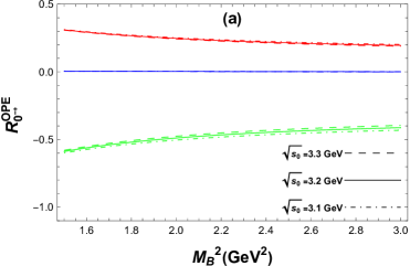
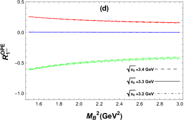
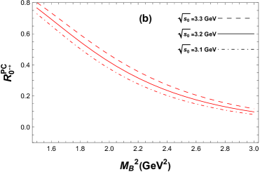
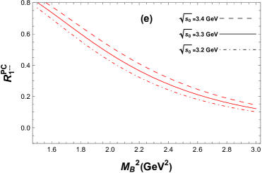
Figure 4: The same caption as in Fig. 1, but for the $\Xi$-$\bar{\Xi}$ states.

For the $\Xi$-$\bar{\Xi}$ states, the ratios $R^{\Xi\bar{\Xi},\;OPE}_{0^{-+}}$ and $R^{\Xi\bar{\Xi},\;PC}_{0^{-+}}$ are shown in Fig. 4(a) and Fig. 4(b) with $\sqrt{s_{0}}=3.1$, $3.2$, and $3.3$ GeV, respectively, and the relationships between $m^{\Xi\bar{\Xi}}_{0^{-+}}$ and parameter $M_{B}^{2}$ are given in Fig. 4(c). The optimal Borel window is found in $2.1\leq M_{B}^{2}\leq 2.8\;\text{GeV}^{2}$, and the mass $m^{\Xi\bar{\Xi}}_{0^{-+}}$ can be obtained as follows:

$$m^{\Xi\bar{\Xi}}_{0^{-+}} = (2.67\pm 0.12)\;\text{GeV}.$$ (25)

The ratios $R^{\Xi\bar{\Xi},\;OPE}_{1^{--}}$ and $R^{\Xi\bar{\Xi},\;PC}_{1^{--}}$ are shown in Fig. 4(d) and Fig. 4(e)with different values of $\sqrt{s_{0}}$, i.e., $3.2$, $3.3$, and $3.4$ GeV, and the relationships between $m^{\Xi\bar{\Xi}}_{1^{--}}$ and parameter $M_{B}^{2}$ are given in Fig. 4(f). The optimal Borel window is found in $2.1\leq M_{B}^{2}\leq 2.9\;\text{GeV}^{2}$, and the mass $m^{\Xi\bar{\Xi}}_{1^{--}}$ can be evaluated as follows:

$$m^{\Xi\bar{\Xi}}_{1^{--}} = (2.79\pm 0.11)\;\text{GeV}.$$ (26)

The errors of the results, (19)$-$(26), mainly stem from the uncertainties in quark masses, condensates, Borel parameter $M_{B}^{2}$ and threshold parameter $\sqrt{s_{0}}$. The nonperturbative contributions by dimensions higher than 12 are also evaluated, and it is less than $10\%$ of dimension 12, so the convergence of OPE makes the high-dimension condensates contributions negligible.

We also analyze the $\mathscr{B}$-$\bar{\mathscr{B}}$ states with the situations of $0^{++}$ and $1^{++}$, and find that no matter what values of $M_{B}^{2}$ and $\sqrt{s_{0}}$ take, no optimal window for stable plateaus exists. That means the currents in Eqs. (3) and (4) do not support the corresponding $\mathscr{B}$-$\bar{\mathscr{B}}$ hexaquark molecular states.

For the convenience of reference, a collection of continuum thresholds, Borel parameters, and predicted masses of hexaquark states are tabulated in Table 1.

Table 1: The continuum thresholds, Borel parameters, and predicted masses of hexaquark molecular states.

$\mathscr{B}$-$\bar{\mathscr{B}}$	$J^{PC}$	$\sqrt{s_{0}}\;(\text{GeV})$	$M_{B}^{2}\;(\text{GeV}^{2})$	$M^{X}\;(\text{GeV})$
$N-\bar{N}$	$0^{-+}$	$2.5\pm 0.1$	$1.6-2.2$	$1.81\pm 0.09$
	$1^{--}$	$2.5\pm 0.1$	$1.6-2.2$	$1.82\pm 0.10$
	$0^{++}$	$...$	$...$	$...$
	$1^{++}$	$...$	$...$	$...$
$\Lambda-\bar{\Lambda}$	$0^{-+}$	$2.9\pm 0.1$	$1.9-2.5$	$2.27\pm 0.13$
	$1^{--}$	$2.9\pm 0.1$	$1.9-2.5$	$2.34\pm 0.12$
	$0^{++}$	$...$	$...$	$...$
	$1^{++}$	$...$	$...$	$...$
$\Sigma-\bar{\Sigma}$	$0^{-+}$	$3.0\pm 0.1$	$2.0-2.6$	$2.39\pm 0.13$
	$1^{--}$	$3.1\pm 0.1$	$2.0-2.6$	$2.48\pm 0.12$
	$0^{++}$	$...$	$...$	$...$
	$1^{++}$	$...$	$...$	$...$
$\Xi-\bar{\Xi}$	$0^{-+}$	$3.2\pm 0.1$	$2.1-2.8$	$2.67\pm 0.12$
	$1^{--}$	$3.3\pm 0.1$	$2.1-2.9$	$2.79\pm 0.11$
	$0^{++}$	$...$	$...$	$...$
	$1^{++}$	$...$	$...$	$...$

IV Decay analyses

To finally ascertain these light baryonium states, the straightforward procedure is to reconstruct them from their decay products, though the detailed characters still ask for more investigation. In our evaluation, the masses of $\Lambda$-$\bar{\Lambda}$, $\Sigma$-$\bar{\Sigma}$, and $\Xi$-$\bar{\Xi}$ states are above the threshold of their respective $\mathscr{B}\bar{\mathscr{B}}$ dibaryons, so the $\Lambda\bar{\Lambda}$, $\Sigma\bar{\Sigma}$, and $\Xi$$\bar{\Xi}$ decay channel will be the primary decay mode, respectively. On the other hand, the masses of $p$-$\bar{p}$ states are below the threshold of $p\bar{p}$ dibaryon, so the $p\bar{p}$ decay channel should be forbidden. The typical decay modes of the light baryonium for different quantum numbers are given in Table 2, and these processes are expected to be measurable in the running experiments like the BESIII, BELLEII, and LHCb.

Table 2: Typical decay modes of the light baryonium for each quantum number.

$J^{PC}$	$N$-$\bar{N}$	$\Lambda$-$\bar{\Lambda}$	$\Sigma$-$\bar{\Sigma}$	$\Xi$-$\bar{\Xi}$
$0^{-+}$	$\pi\pi\pi$	$\Lambda\bar{\Lambda}$	$\Sigma\bar{\Sigma}$	$\Xi\bar{\Xi}$   $\eta KK$
	$\pi\pi\eta$	$\pi\pi\eta$	$\pi\pi\eta$	$\eta\eta\pi$   $\eta^{\prime}KK$
	$\pi\pi\eta^{\prime}$	$\pi\pi\eta^{\prime}$	$\pi\pi\eta^{\prime}$	$\eta^{\prime}\eta^{\prime}\pi$
		$\pi KK$	$\pi KK$	$\eta\eta^{\prime}\pi$
$1^{--}$	$\pi\pi\omega$	$\Lambda\bar{\Lambda}$	$\Sigma\bar{\Sigma}$	$\Xi\bar{\Xi}$   $\omega KK$
	$\pi\pi\phi$	$\pi\pi\omega$	$\pi\pi\omega$	$\phi\phi\pi$   $\phi KK$
		$\pi\pi\phi$	$\pi\pi\phi$	$\omega\omega\pi$
		$\pi K^{\ast}K^{\ast}$	$\pi K^{\ast}K^{\ast}$	$\omega\phi\pi$

V Conclusions

In summary, we investigate the light baryonium states in molecular configuration with quantum numbers of $J^{PC}=0^{-+}$, $1^{--}$, $0^{++}$, and $1^{++}$ in the framework of QCD sum rules. Our results suggest that there exist eight possible light baryonium states, i.e., $p$-$\bar{p}$, $\Lambda$-$\bar{\Lambda}$, $\Sigma$-$\bar{\Sigma}$, and $\Xi$-$\bar{\Xi}$ with quantum numbers of $0^{-+}$ and $1^{--}$, and their masses are tabulated in Table 1. According to our evaluation, the masses of $\Lambda$-$\bar{\Lambda}$, $\Sigma$-$\bar{\Sigma}$, and $\Xi$-$\bar{\Xi}$ states are above their corresponding dibaryon thresholds, while the masses of $p$-$\bar{p}$ states are not. Moreover, the primary and potential decay modes of these light baryonium states are analyzed, which might serve as a guide for experimental exploration in BESIII, BELLEII, or LHCb.

Acknowledgments

This work was supported in part by the National Key Research and Development Program of China under Contract No. 2020YFA0406400, and the National Natural Science Foundation of China (NSFC) under the Grants No. 11975236 and No. 11635009.

Appendix A The spectral densities $\mathscr{B}$-$\bar{\mathscr{B}}$ hexaquark states

A.1 The spectral densities of $0^{-+}$ $p$-$\bar{p}$ hexaquark states

The $0^{-+}$ $p$-$\bar{p}$ hexaquark state spectral densities on the OPE side can be expressed as:

$$\Pi_{0^{-+}}^{p\bar{p}}(s_{0},M_{B}^{2})=\int_{s_{min}}^{s_{0}}\;e^{-s/M_{B}^{2}}\;\sum_{n}\;c_{n}\;s^{n}\;ds+\Pi^{sum}(M_{B}^{2})\;.$$ (27)

Here,

$$c_{7} = \frac{1}{2^{23}\times 3^{2}\times 5^{2}\times 7^{2}\;\pi^{10}}\;,$$ (28)

$$c_{6} = \frac{m_{u}\left(2m_{d}+m_{u}\right)}{2^{20}\times 3^{2}\times 5^{2}\times 7\;\pi^{10}}\;,$$ (29)

$$c_{5} = \frac{m_{d}\left(m_{d}+2m_{u}\right)m_{u}^{2}}{2^{19}\times 3\times 5^{2}\,\pi^{10}}-\frac{\left\langle\bar{q}q\right\rangle\left(m_{d}+2m_{u}\right)}{2^{17}\times 3^{2}\times 5^{2}\,\pi^{8}}+\frac{\left\langle GG\right\rangle}{2^{22}\times 3^{2}\times 5^{2}\,\pi^{10}}\;,$$ (30)

$$c_{4} = \frac{\left\langle GG\right\rangle\left(m_{d}+m_{u}\right)m_{u}}{2^{21}\times 3\times 5\,\pi^{10}}-\frac{\left\langle\bar{q}q\right\rangle\left(m_{d}^{2}+4m_{u}m_{d}+m_{u}^{2}\right)m_{u}}{2^{16}\times 3\times 5\,\pi^{8}}$$ (31)

$$+ \frac{m_{d}^{2}m_{u}^{4}}{2^{18}\times 5\,\pi^{10}}+\frac{\left\langle\bar{q}Gq\right\rangle\left(m_{d}+2m_{u}\right)}{2^{17}\times 3\times 5\,\pi^{8}}+\frac{\left\langle\bar{q}q\right\rangle^{2}}{2^{14}\times 3\times 5\,\pi^{6}}\;,$$

$$c_{3} = \frac{\left\langle GG\right\rangle m_{d}m_{u}^{3}}{2^{19}\times 3\,\pi^{10}}+\frac{\left\langle\bar{q}Gq\right\rangle\left(m_{d}^{2}+4m_{u}m_{d}+m_{u}^{2}\right)m_{u}}{2^{15}\times 3\,\pi^{8}}-\left\langle\bar{q}q\right\rangle\bigg{[}\frac{m_{d}\left(2m_{d}+m_{u}\right)m_{u}^{3}}{2^{14}\times 3\,\pi^{8}}$$ (32)

$$+ \frac{\left\langle\bar{q}Gq\right\rangle}{2^{13}\times 3\,\pi^{6}}+\frac{\left\langle GG\right\rangle\left(m_{d}+3m_{u}\right)}{2^{18}\times 3^{2}\,\pi^{8}}\bigg{]}+\frac{\left\langle\bar{q}q\right\rangle^{2}\left(m_{d}^{2}+24m_{u}m_{d}+14m_{u}^{2}\right)}{2^{14}\times 3^{2}\,\pi^{6}}\;,$$

$$c_{2} = -\frac{\left(m_{d}+2m_{u}\right)\left\langle\bar{q}q\right\rangle^{3}}{2^{7}\times 3^{2}\,\pi^{4}}+\bigg{[}\frac{\left(11m_{d}^{2}+18m_{u}m_{d}+m_{u}^{2}\right)m_{u}^{2}}{2^{12}\times 3\,\pi^{6}}+\frac{\left\langle GG\right\rangle}{2^{12}\times 3^{2}\,\pi^{6}}\bigg{]}\left\langle\bar{q}q\right\rangle^{2}$$ (33)

$$+ \bigg{[}-\frac{\left\langle GG\right\rangle\left(3m_{d}+m_{u}\right)m_{u}^{2}}{2^{16}\times 3\,\pi^{8}}-\frac{\left\langle\bar{q}Gq\right\rangle\left(m_{d}^{2}+14m_{u}m_{d}+9m_{u}^{2}\right)}{2^{12}\times 3\,\pi^{6}}\bigg{]}\left\langle\bar{q}q\right\rangle$$

$$+ \frac{\left\langle\bar{q}Gq\right\rangle m_{d}m_{u}^{3}\left(2m_{d}+m_{u}\right)}{2^{13}\,\pi^{8}}+\frac{\left\langle GG\right\rangle\left\langle\bar{q}Gq\right\rangle\left(m_{d}+3m_{u}\right)}{2^{17}\times 3\,\pi^{8}}+\frac{\left\langle\bar{q}Gq\right\rangle^{2}}{2^{14}\,\pi^{6}}\;,$$

$$c_{1} = \frac{\left\langle\bar{q}q\right\rangle^{4}}{2^{5}\times 3\,\pi^{2}}-\frac{m_{u}\left(3m_{d}^{2}+11m_{u}m_{d}+3m_{u}^{2}\right)\left\langle\bar{q}q\right\rangle^{3}}{2^{8}\times 3\,\pi^{4}}$$ (34)

$$+ \left[\frac{3m_{d}^{2}m_{u}^{4}}{2^{11}\,\pi^{6}}+\frac{7\left\langle GG\right\rangle\left(m_{d}+m_{u}\right)m_{u}}{2^{14}\times 3\,\pi^{6}}+\frac{\left\langle\bar{q}Gq\right\rangle\left(m_{d}+2m_{u}\right)}{2^{6}\times 3\,\pi^{4}}\right]\left\langle\bar{q}q\right\rangle^{2}$$

$$+ \left[-\frac{\left\langle\bar{q}Gq\right\rangle\left(7m_{d}^{2}+10m_{u}m_{d}+m_{u}^{2}\right)m_{u}^{2}}{2^{11}\,\pi^{6}}-\frac{\left\langle GG\right\rangle\left\langle\bar{q}Gq\right\rangle}{2^{12}\times 3\,\pi^{6}}\right]\left\langle\bar{q}q\right\rangle$$

$$+ \frac{\left\langle GG\right\rangle\left\langle\bar{q}Gq\right\rangle m_{u}^{2}\left(3m_{d}+m_{u}\right)}{2^{16}\,\pi^{8}}+\frac{\left\langle\bar{q}Gq\right\rangle^{2}\left(m_{d}^{2}+10m_{u}m_{d}+7m_{u}^{2}\right)}{2^{13}\,\pi^{6}}\;,$$

$$c_{0} = \left\langle\bar{q}q\right\rangle^{2}\left[\frac{\left\langle GG\right\rangle m_{d}m_{u}^{3}}{2^{12}\times 3\,\pi^{6}}+\frac{\left\langle\bar{q}Gq\right\rangle\left(2m_{d}^{2}+7m_{u}m_{d}+2m_{u}^{2}\right)m_{u}}{2^{8}\,\pi^{4}}\right]$$ (35)

$$+ \frac{\left\langle\bar{q}Gq\right\rangle^{2}m_{u}^{2}\left(6m_{d}^{2}+8m_{u}m_{d}+m_{u}^{2}\right)}{2^{12}\,\pi^{6}}+\frac{\left\langle\bar{q}q\right\rangle^{4}\left(m_{d}^{2}+18m_{u}m_{d}+11m_{u}^{2}\right)}{2^{6}\times 3^{2}\,\pi^{2}}$$

$$- \frac{m_{d}m_{u}^{3}\left\langle\bar{q}q\right\rangle^{3}\left(2m_{d}+m_{u}\right)}{2^{7}\times 3\,\pi^{4}}-\frac{m_{u}\left\langle\bar{q}q\right\rangle\left\langle GG\right\rangle\left\langle\bar{q}Gq\right\rangle\left(m_{d}+m_{u}\right)}{2^{11}\times 3\,\pi^{6}}\;,$$

and $\Pi^{sum}$ is the sum of those contributions in the correlation function that have no imaginary part but are nontrivial after the Borel transformation, and

$$\Pi^{sum}(M_{B}^{2})=\frac{\left\langle\bar{q}q\right\rangle^{4}m_{u}^{2}\left(24m_{d}m_{u}+14m_{d}^{2}+m_{u}^{2}\right)}{2^{8}\times 3^{2}\,\pi^{2}}+\frac{\left\langle\bar{q}q\right\rangle^{2}\left\langle\bar{q}Gq\right\rangle m_{d}m_{u}^{3}\left(2m_{d}+m_{u}\right)}{2^{8}\times 3\,\pi^{4}}\;.$$ (36)

A.2 The spectral densities of $0^{++}$ $p$-$\bar{p}$ hexaquark states

The $0^{++}$ $p$-$\bar{p}$ hexaquark state spectral densities on the OPE side can be expressed as:

$$c_{7} = -\frac{1}{2^{23}\times 3^{2}\times 5^{2}\times 7^{2}\,\pi^{10}}\;,$$ (37)

$$c_{6} = \frac{m_{u}\left(m_{u}-2m_{d}\right)}{2^{20}\times 3^{2}\times 5^{2}\times 7^{1}\,\pi^{10}}\;,$$ (38)

$$c_{5} = \frac{\left\langle\bar{q}q\right\rangle\left(m_{d}-2m_{u}\right)}{2^{17}\times 3^{2}\times 5^{2}\,\pi^{8}}+\frac{m_{u}^{2}\left(2m_{d}m_{u}-m_{d}^{2}\right)}{2^{19}\times 3\times 5^{2}\,\pi^{10}}-\frac{\left\langle GG\right\rangle^{2}}{2^{22}\times 3^{2}\times 5^{2}\,\pi^{10}}\;,$$ (39)

$$c_{4} = \frac{\left\langle\bar{q}q\right\rangle m_{u}\left(m_{d}^{2}-m_{u}\left(6m_{d}+m_{u}\right)\right)}{2^{16}\times 3\times 5\,\pi^{8}}+\frac{\left\langle GG\right\rangle^{2}m_{u}\left(m_{u}-m_{d}\right)}{2^{21}\times 3\times 5\,\pi^{10}}$$ (40)

$$- \frac{\left\langle\bar{q}Gq\right\rangle m_{d}}{2^{17}\times 3\times 5\,\pi^{8}}+\frac{9m_{d}^{2}m_{u}^{4}-16\pi^{4}\left\langle\bar{q}q\right\rangle^{2}}{2^{18}\times 3^{2}\times 5\,\pi^{10}}\;,$$

$$c_{3} = \left\langle\bar{q}q\right\rangle\left[\frac{\left\langle GG\right\rangle^{2}\left(m_{d}-5m_{u}\right)}{2^{18}\times 3^{2}\,\pi^{8}}-\frac{m_{u}^{3}\left(m_{d}m_{u}+4m_{d}^{2}\right)}{2^{14}\times 3\,\pi^{8}}\right]$$ (41)

$$+ \frac{\left\langle GG\right\rangle^{2}m_{d}m_{u}^{3}}{2^{19}\times 3\,\pi^{10}}+\frac{\left\langle\bar{q}Gq\right\rangle m_{u}\left(2m_{d}m_{u}-m_{d}^{2}+m_{u}^{2}\right)}{2^{15}\times 3\,\pi^{8}}$$

$$+ \frac{2\left\langle\bar{q}q\right\rangle^{2}m_{u}\left(4m_{d}+9m_{u}\right)+\left\langle\bar{q}q\right\rangle^{2}\left(-m_{d}^{2}\right)+2\left\langle\bar{q}q\right\rangle\left\langle\bar{q}Gq\right\rangle}{2^{14}\times 3^{2}\,\pi^{6}}\;,$$

$$c_{2} = -\frac{\left\langle\bar{q}q\right\rangle\left\langle GG\right\rangle^{2}m_{u}^{2}\left(7m_{d}+m_{u}\right)}{2^{16}\times 3\,\pi^{8}}+\frac{\left\langle GG\right\rangle^{2}\left\langle\bar{q}Gq\right\rangle\left(m_{u}-m_{d}\right)}{2^{17}\times 3\,\pi^{8}}+\frac{\left\langle\bar{q}Gq\right\rangle m_{u}^{3}\left(m_{d}m_{u}+2m_{d}^{2}\right)}{2^{13}\,\pi^{8}}$$ (42)

$$+ \frac{1}{2^{12}\times 3\,\pi^{6}}\bigg{[}m_{u}^{2}\left(15\left\langle\bar{q}q\right\rangle^{2}m_{d}^{2}-11\left\langle\bar{q}q\right\rangle\left\langle\bar{q}Gq\right\rangle\right)+m_{d}\left(22\left\langle\bar{q}q\right\rangle^{2}m_{u}^{3}-6\left\langle\bar{q}q\right\rangle\left\langle\bar{q}Gq\right\rangle m_{u}\right)$$

$$+ \left\langle\bar{q}q\right\rangle\left\langle\bar{q}Gq\right\rangle m_{d}^{2}+\left\langle\bar{q}q\right\rangle^{2}m_{u}^{4}\bigg{]}-\frac{\left\langle\bar{q}q\right\rangle^{3}m_{u}}{2^{7}\times 3\,\pi^{4}}-\frac{\left\langle\bar{q}Gq\right\rangle^{2}}{2^{14}\times 3\,\pi^{6}}\;,$$

$$c_{1} = -\frac{\left\langle\bar{q}q\right\rangle^{3}m_{u}\left(7m_{d}m_{u}+m_{d}^{2}+m_{u}^{2}\right)}{2^{8}\,\pi^{4}}+\left\langle\bar{q}q\right\rangle^{2}\left[\frac{3\left\langle GG\right\rangle^{2}m_{u}\left(m_{d}+m_{u}\right)}{2^{14}\,\pi^{6}}+\frac{\left\langle\bar{q}Gq\right\rangle m_{u}}{2^{5}\times 3\,\pi^{4}}\right]$$ (43)

$$+ \frac{\left\langle GG\right\rangle^{2}\left\langle\bar{q}Gq\right\rangle m_{u}^{2}\left(3m_{d}+m_{u}\right)}{2^{16}\,\pi^{8}}-\frac{\left\langle\bar{q}Gq\right\rangle^{2}\left(-2m_{d}m_{u}+m_{d}^{2}-5m_{u}^{2}\right)}{2^{13}\,\pi^{6}}+\frac{\left\langle\bar{q}q\right\rangle^{4}}{2^{5}\times 3^{2}\,\pi^{2}}$$

$$+ \frac{m_{u}^{2}\left[m_{u}^{2}(\left\langle\bar{q}q\right\rangle^{2}m_{d}^{2}-\left\langle\bar{q}q\right\rangle\left\langle\bar{q}Gq\right\rangle)-14\left\langle\bar{q}q\right\rangle\left\langle\bar{q}Gq\right\rangle m_{d}m_{u}-11\left\langle\bar{q}q\right\rangle\left\langle\bar{q}Gq\right\rangle m_{d}^{2}\right]}{2^{11}\,\pi^{6}}\;,$$

$$c_{0} = \frac{\left\langle\bar{q}q\right\rangle^{4}\left(22m_{d}m_{u}+m_{d}^{2}+15m_{u}^{2}\right)}{2^{6}\times 3^{2}\,\pi^{2}}-\frac{\left\langle\bar{q}q\right\rangle^{3}m_{d}^{2}m_{u}^{3}}{2^{7}\,\pi^{4}}-\frac{\left\langle\bar{q}q\right\rangle\left\langle GG\right\rangle^{2}\left\langle\bar{q}Gq\right\rangle m_{u}\left(m_{d}+m_{u}\right)}{2^{12}\,\pi^{6}}$$

$$+ \frac{\left\langle\bar{q}q\right\rangle^{2}\left\langle\bar{q}Gq\right\rangle m_{u}\left(31m_{d}m_{u}+7m_{d}^{2}+7m_{u}^{2}\right)}{2^{8}\times 3\,\pi^{4}}+\frac{\left\langle\bar{q}Gq\right\rangle^{2}m_{u}^{2}\left(8m_{d}m_{u}+6m_{d}^{2}+m_{u}^{2}\right)}{2^{12}\,\pi^{6}}\;,$$

and

$$\Pi^{sum}(M_{B}^{2})=\frac{\left\langle\bar{q}q\right\rangle^{2}\left\langle\bar{q}Gq\right\rangle\left(m_{d}^{2}m_{u}^{3}\right)}{2^{8}\times 3\,\pi^{4}}+\left\langle\bar{q}q\right\rangle^{4}\left(\frac{m_{d}m_{u}^{3}}{2^{5}\times 3^{2}\,\pi^{2}}++\frac{m_{d}^{2}m_{u}^{2}}{2^{7}\,\pi^{2}}-\frac{m_{u}^{4}}{2^{8}\times 3^{2}\,\pi^{2}}\right)\;.$$ (45)

A.3 The spectral densities of $1^{--}$ $p$-$\bar{p}$ hexaquark states

The $1^{--}$ $p$-$\bar{p}$ hexaquark state spectral densities on the OPE side can be expressed as:

$$c_{7} = -\frac{1}{2^{20}\times 3^{4}\times 5^{2}\times 7^{2}\,\pi^{10}}\;,$$ (46)

$$c_{6} = -\frac{m_{u}\left(7m_{d}+4m_{u}\right)}{2^{22}\times 3^{2}\times 5^{2}\times 7\,\pi^{10}}\;,$$ (47)

$$c_{5} = \frac{\left\langle\bar{q}q\right\rangle\left(3m_{d}+7m_{u}\right)}{2^{16}\times 3^{2}\times 5^{2}\times 7\,\pi^{8}}-\frac{m_{d}m_{u}^{2}\left(3m_{d}+7m_{u}\right)}{2^{18}\times 3\times 5^{2}\times 7\,\pi^{10}}-\frac{\left\langle GG\right\rangle}{2^{21}\times 3\times 5^{2}\times 7\,\pi^{10}}\;,$$ (48)

$$c_{4} = \frac{\left\langle\bar{q}q\right\rangle m_{u}\left(25m_{d}m_{u}+5m_{d}^{2}+6m_{u}^{2}\right)}{2^{17}\times 3^{2}\times 5\,\pi^{8}}-\frac{\left\langle GG\right\rangle m_{u}\left(5m_{d}+6m_{u}\right)}{2^{22}\times 3^{2}\times 5\,\pi^{10}}$$ (49)

$$- \frac{\left\langle\bar{q}Gq\right\rangle\left(5m_{d}+11m_{u}\right)}{2^{18}\times 3^{2}\times 5\,\pi^{8}}-\frac{m_{d}^{2}m_{u}^{4}}{2^{18}\times 5\,\pi^{10}}-\frac{\left\langle\bar{q}q\right\rangle^{2}}{2^{11}\times 3^{3}\times 5\,\pi^{6}}\;,$$

$$c_{3} = -\frac{\left\langle\bar{q}q\right\rangle^{2}\left(28m_{d}m_{u}+m_{d}^{2}+18m_{u}^{2}\right)}{2^{12}\times 3^{2}\times 5\,\pi^{6}}$$ (50)

$$+ \left\langle\bar{q}q\right\rangle\left[\frac{\left\langle GG\right\rangle\left(m_{d}+4m_{u}\right)}{2^{16}\times 3^{2}\times 5\,\pi^{8}}+\frac{m_{d}m_{u}^{3}\left(11m_{d}+5m_{u}\right)}{2^{14}\times 3\times 5\,\pi^{8}}+\frac{13\left\langle\bar{q}Gq\right\rangle}{2^{13}\times 3^{2}\times 5\,\pi^{6}}\right]$$

$$- \frac{\left\langle GG\right\rangle m_{d}m_{u}^{3}}{2^{19}\times 3\,\pi^{10}}-\frac{\left\langle\bar{q}Gq\right\rangle m_{u}\left(19m_{d}m_{u}+4m_{d}^{2}+5m_{u}^{2}\right)}{2^{15}\times 3\times 5\,\pi^{8}}\;,$$

$$c_{2} = \frac{\left\langle\bar{q}q\right\rangle^{3}\left(7m_{d}+17m_{u}\right)}{2^{10}\times 3^{2}\,\pi^{4}}+\left\langle\bar{q}q\right\rangle^{2}\left[-\frac{m_{u}^{2}\left(37m_{d}m_{u}+23m_{d}^{2}+2m_{u}^{2}\right)}{2^{13}\times 3\,\pi^{6}}-\frac{7\left\langle GG\right\rangle}{2^{15}\times 3^{2}\,\pi^{6}}\right]$$ (51)

$$+ \left\langle\bar{q}q\right\rangle\left[\frac{\left\langle GG\right\rangle m_{u}^{2}\left(7m_{d}+2m_{u}\right)}{2^{17}\times 3\,\pi^{8}}+\frac{\left\langle\bar{q}Gq\right\rangle\left(52m_{d}m_{u}+3m_{d}^{2}+37m_{u}^{2}\right)}{2^{14}\times 3\,\pi^{6}}\right]$$

$$- \frac{\left\langle\bar{q}Gq\right\rangle m_{d}m_{u}^{3}\left(2m_{d}+m_{u}\right)}{2^{13}\,\pi^{8}}-\frac{5\left\langle\bar{q}Gq\right\rangle^{2}}{2^{15}\times 3\,\pi^{6}}-\frac{\left\langle GG\right\rangle\left\langle\bar{q}Gq\right\rangle\left(3m_{d}+11m_{u}\right)}{2^{19}\times 3\,\pi^{8}}\;,$$

$$c_{1} = \frac{\left\langle\bar{q}q\right\rangle^{3}m_{u}\left(38m_{d}m_{u}+9m_{d}^{2}+9m_{u}^{2}\right)}{2^{8}\times 3^{2}\,\pi^{4}}-\frac{\left\langle GG\right\rangle\left\langle\bar{q}Gq\right\rangle m_{u}^{2}\left(3m_{d}+m_{u}\right)}{2^{16}\,\pi^{8}}$$ (52)

$$+ \left\langle\bar{q}q\right\rangle^{2}\left[-\frac{11\left\langle GG\right\rangle m_{u}\left(m_{d}+m_{u}\right)}{2^{13}\times 3^{2}\,\pi^{6}}-\frac{\left\langle\bar{q}Gq\right\rangle\left(5m_{d}+12m_{u}\right)}{2^{7}\times 3^{2}\,\pi^{4}}-\frac{m_{d}^{2}m_{u}^{4}}{2^{8}\times 3\,\pi^{6}}\right]$$

$$+ \left\langle\bar{q}q\right\rangle\left[\frac{\left\langle\bar{q}Gq\right\rangle m_{u}^{2}\left(32m_{d}m_{u}+23m_{d}^{2}+3m_{u}^{2}\right)}{2^{11}\times 3\,\pi^{6}}+\frac{5\left\langle GG\right\rangle\left\langle\bar{q}Gq\right\rangle}{2^{13}\times 3^{2}\,\pi^{6}}\right]$$

$$- \frac{\left\langle\bar{q}Gq\right\rangle^{2}\left(13m_{d}m_{u}+m_{d}^{2}+10m_{u}^{2}\right)}{2^{12}\times 3\,\pi^{6}}-\frac{\left\langle\bar{q}q\right\rangle^{4}}{2^{2}\times 3^{3}\,\pi^{2}}\;,$$

$$c_{0} = -\frac{\left\langle\bar{q}q\right\rangle^{4}\left(19m_{d}m_{u}+m_{d}^{2}+12m_{u}^{2}\right)}{2^{6}\times 3^{2}\,\pi^{2}}+\frac{\left\langle\bar{q}q\right\rangle^{3}m_{d}m_{u}^{3}\left(3m_{d}+m_{u}\right)}{2^{9}\,\pi^{4}}$$ (53)

$$+ \left\langle\bar{q}q\right\rangle^{2}\left[-\frac{\left\langle GG\right\rangle m_{d}m_{u}^{3}}{2^{14}\,\pi^{6}}-\frac{\left\langle\bar{q}Gq\right\rangle m_{u}\left(94m_{d}m_{u}+25m_{d}^{2}+25m_{u}^{2}\right)}{2^{10}\times 3\,\pi^{4}}\right]$$

$$+ \frac{3\left\langle\bar{q}q\right\rangle\left\langle GG\right\rangle\left\langle\bar{q}Gq\right\rangle m_{u}\left(m_{d}+m_{u}\right)}{2^{14}\,\pi^{6}}-\frac{\left\langle\bar{q}Gq\right\rangle^{2}m_{u}^{2}\left(8m_{d}m_{u}+6m_{d}^{2}+m_{u}^{2}\right)}{2^{12}\,\pi^{6}}\;,$$

and

$$\Pi^{sum}(M_{B}^{2})=\left\langle\bar{q}q\right\rangle^{4}\left(\frac{m_{d}m_{u}^{3}}{2^{5}\times 3^{2}\,\pi^{2}}+\frac{m_{d}^{2}m_{u}^{2}}{2^{7}\,\pi^{2}}-\frac{m_{u}^{4}}{2^{8}\times 3^{2}\,\pi^{2}}\right)+\frac{\left\langle\bar{q}q\right\rangle^{2}\left\langle\bar{q}Gq\right\rangle\left(m_{d}^{2}m_{u}^{3}\right)}{2^{8}\times 3\,\pi^{4}}\;.$$ (54)

A.4 The spectral densities of $1^{++}$ $p$-$\bar{p}$ hexaquark states

The $1^{++}$ $p$-$\bar{p}$ hexaquark state spectral densities on the OPE side can be expressed as:

$$c_{7} = -\frac{1}{2^{20}\times 3^{4}\times 5^{2}\times 7^{2}\,\pi^{10}}\;,$$ (55)

$$c_{6} = -\frac{m_{u}\left(7m_{d}+4m_{u}\right)}{2^{22}\times 3^{2}\times 5^{2}\times 7\,\pi^{10}}\;,$$ (56)

$$c_{5} = \frac{\left\langle\bar{q}q\right\rangle\left(3m_{d}+7m_{u}\right)}{2^{16}\times 3^{2}\times 5^{2}\times 7\,\pi^{8}}-\frac{m_{d}m_{u}^{2}\left(3m_{d}+7m_{u}\right)}{2^{18}\times 3\times 5^{2}\times 7\,\pi^{10}}-\frac{\left\langle GG\right\rangle^{2}}{2^{21}\times 3\times 5^{2}\times 7\,\pi^{10}}\;,$$ (57)

$$c_{4} = \frac{\left\langle\bar{q}q\right\rangle m_{u}\left(25m_{d}m_{u}+5m_{d}^{2}+6m_{u}^{2}\right)}{2^{17}\times 3^{2}\times 5\,\pi^{8}}-\frac{\left\langle GG\right\rangle^{2}m_{u}\left(5m_{d}+6m_{u}\right)}{2^{22}\times 3^{2}\times 5\,\pi^{10}}$$ (58)

$$- \frac{\left\langle\bar{q}Gq\right\rangle\left(5m_{d}+11m_{u}\right)}{2^{18}\times 3^{2}\times 5\,\pi^{8}}-\frac{27m_{d}^{2}m_{u}^{4}+2^{7}\,\pi^{4}\left\langle\bar{q}q\right\rangle^{2}}{2^{18}\times 3^{3}\times 5\,\pi^{10}}\;,$$

$$c_{3} = \left\langle\bar{q}q\right\rangle\left[\frac{\left\langle GG\right\rangle^{2}\left(m_{d}+4m_{u}\right)}{2^{16}\times 3^{2}\times 5\,\pi^{8}}+\frac{m_{d}m_{u}^{3}\left(11m_{d}+5m_{u}\right)}{2^{14}\times 3\times 5\,\pi^{8}}+\frac{13\left\langle\bar{q}Gq\right\rangle}{2^{13}\times 3^{2}\times 5\,\pi^{6}}\right]-\frac{\left\langle GG\right\rangle^{2}m_{d}m_{u}^{3}}{2^{19}\times 3\,\pi^{10}}$$ (59)

$$- \frac{\left\langle\bar{q}Gq\right\rangle m_{u}\left(19m_{d}m_{u}+4m_{d}^{2}+5m_{u}^{2}\right)}{2^{15}\times 3\times 5\,\pi^{8}}-\frac{\left\langle\bar{q}q\right\rangle^{2}\left(28m_{d}m_{u}+m_{d}^{2}+18m_{u}^{2}\right)}{2^{12}\times 3^{2}\times 5\,\pi^{6}}\;,$$

$$c_{2} = \frac{\left\langle\bar{q}q\right\rangle^{3}\left(7m_{d}+17m_{u}\right)}{2^{10}\times 3^{2}\,\pi^{4}}-\frac{7\left\langle\bar{q}q\right\rangle^{2}\left\langle GG\right\rangle^{2}}{2^{15}\times 3^{2}\,\pi^{6}}-\frac{5\left\langle\bar{q}Gq\right\rangle^{2}}{2^{15}\times 3\,\pi^{6}}-\frac{\left\langle\bar{q}Gq\right\rangle m_{d}m_{u}^{3}\left(2m_{d}+m_{u}\right)}{2^{13}\,\pi^{8}}$$ (60)

$$+ \left\langle\bar{q}q\right\rangle\left[\left\langle GG\right\rangle^{2}\left(\frac{m_{u}^{2}\left(7m_{d}+2m_{u}\right)}{2^{17}\times 3\,\pi^{8}}-\frac{7\left\langle\bar{q}Gq\right\rangle}{2^{15}\times 3^{2}\,\pi^{6}}\right)+\frac{\left\langle\bar{q}Gq\right\rangle\left(52m_{d}m_{u}+3m_{d}^{2}+37m_{u}^{2}\right)}{2^{14}\times 3\,\pi^{6}}\right]$$

$$- \frac{\left\langle GG\right\rangle^{2}\left\langle\bar{q}Gq\right\rangle\left(3m_{d}+11m_{u}\right)}{2^{19}\times 3\,\pi^{8}}-\frac{\left\langle\bar{q}q\right\rangle^{2}m_{u}^{2}\left(37m_{d}m_{u}+23m_{d}^{2}+2m_{u}^{2}\right)}{2^{13}\times 3\,\pi^{6}}\;,$$

$$c_{1} = \frac{\left\langle\bar{q}q\right\rangle^{3}m_{u}\left(38m_{d}m_{u}+9m_{d}^{2}+9m_{u}^{2}\right)}{2^{8}\times 3^{2}\,\pi^{4}}+\left\langle\bar{q}q\right\rangle^{2}\big{(}-\frac{11\left\langle GG\right\rangle^{2}m_{u}\left(m_{d}+m_{u}\right)}{2^{13}\times 3^{2}\,\pi^{6}}$$ (61)

$$- \frac{\left\langle\bar{q}Gq\right\rangle\left(5m_{d}+12m_{u}\right)}{2^{7}\times 3^{2}\,\pi^{4}}\big{)}+\left\langle\bar{q}q\right\rangle\bigg{[}\frac{\left\langle\bar{q}Gq\right\rangle m_{u}^{2}\left(32m_{d}m_{u}+23m_{d}^{2}+3m_{u}^{2}\right)}{2^{11}\times 3\,\pi^{6}}$$

$$- \frac{11\left\langle GG\right\rangle^{2}\left\langle\bar{q}Gq\right\rangle m_{u}\left(m_{d}+m_{u}\right)}{2^{13}\times 3^{2}\,\pi^{6}}\bigg{]}-\frac{\left\langle\bar{q}q\right\rangle^{4}}{2^{2}\times 3^{3}\,\pi^{2}}$$

$$- \frac{\left\langle GG\right\rangle^{2}\left\langle\bar{q}Gq\right\rangle m_{u}^{2}\left(3m_{d}+m_{u}\right)}{2^{16}\,\pi^{8}}-\frac{\left\langle\bar{q}Gq\right\rangle^{2}\left(13m_{d}m_{u}+m_{d}^{2}+10m_{u}^{2}\right)}{2^{12}\times 3\,\pi^{6}}-\frac{\left\langle\bar{q}q\right\rangle^{2}m_{d}^{2}m_{u}^{4}}{2^{8}\times 3\,\pi^{6}}\;,$$

$$c_{0} = -\frac{\left\langle\bar{q}q\right\rangle^{4}\left(19m_{d}m_{u}+m_{d}^{2}+12m_{u}^{2}\right)}{2^{6}\times 3^{2}\,\pi^{2}}+\frac{\left\langle\bar{q}q\right\rangle^{3}m_{d}m_{u}^{3}\left(3m_{d}+m_{u}\right)}{2^{9}\,\pi^{4}}$$ (62)

$$+ \left\langle\bar{q}q\right\rangle^{2}\left[-\frac{\left\langle GG\right\rangle^{2}m_{d}m_{u}^{3}}{2^{14}\,\pi^{6}}-\frac{\left\langle\bar{q}Gq\right\rangle m_{u}\left(94m_{d}m_{u}+25m_{d}^{2}+25m_{u}^{2}\right)}{2^{10}\times 3\,\pi^{4}}\right]$$

$$- \frac{\left\langle\bar{q}q\right\rangle\left\langle GG\right\rangle^{2}\left\langle\bar{q}Gq\right\rangle m_{d}m_{u}^{3}}{2^{14}\,\pi^{6}}-\frac{\left\langle\bar{q}Gq\right\rangle^{2}m_{u}^{2}\left(8m_{d}m_{u}+6m_{d}^{2}+m_{u}^{2}\right)}{2^{12}\,\pi^{6}}\;,$$

and

$$\Pi^{sum}(M_{B}^{2}) = \left\langle\bar{q}q\right\rangle^{2}\left\langle\bar{q}Gq\right\rangle\left(-\frac{m_{d}m_{u}^{4}}{2^{9}\times 3\,\pi^{4}}-\frac{m_{d}^{2}m_{u}^{3}}{2^{9}\,\pi^{4}}\right)$$ (63)

$$+ \frac{\left\langle\bar{q}q\right\rangle^{4}\left(m_{d}m_{u}^{2}\left(m_{d}+m_{u}\right)\right)}{2^{7}\times 3^{2}\,\pi^{2}}\;.$$

A.5 The spectral densities of $0^{-+}$ $\Lambda$-$\bar{\Lambda}$ hexaquark states

The $0^{-+}$ $\Lambda$-$\bar{\Lambda}$ hexaquark state spectral densities on the OPE side can be expressed as:

$$c_{7} = \frac{1}{2^{23}\times 3^{2}\times 5^{2}\times 7^{2}\,\pi^{10}}\;,$$ (64)

$$c_{6} = \frac{m_{s}^{2}}{2^{20}\times 3^{2}\times 5^{2}\times 7\,\pi^{10}}\;,$$ (65)

$$c_{5} = \frac{\left\langle GG\right\rangle}{2^{22}\times 3^{2}\times 5^{2}\,\pi^{10}}-\frac{\left\langle\bar{s}s\right\rangle m_{s}}{2^{17}\times 3^{2}\times 5^{2}\,\pi^{8}}\;,$$ (66)

$$c_{4} = \frac{\left\langle GG\right\rangle m_{s}^{2}}{2^{21}\times 3\times 5\,\pi^{10}}+\frac{\left\langle\bar{s}Gs\right\rangle m_{s}}{2^{17}\times 3\times 5\,\pi^{8}}+\frac{\left\langle\bar{q}q\right\rangle^{2}}{2^{13}\times 3^{2}\times 5\,\pi^{6}}+\frac{\left\langle\bar{s}s\right\rangle^{2}}{2^{14}\times 3^{2}\times 5\,\pi^{6}}\;,$$ (67)

$$c_{3} = \frac{\left\langle\bar{q}q\right\rangle^{2}m_{s}^{2}}{2^{11}\times 3^{2}\,\pi^{6}}+\frac{\left\langle\bar{s}s\right\rangle^{2}m_{s}^{2}}{2^{14}\times 3^{2}\,\pi^{6}}-\frac{\left\langle\bar{s}s\right\rangle\left\langle GG\right\rangle m_{s}}{2^{17}\times 3^{2}\,\pi^{8}}-\frac{\left\langle\bar{q}q\right\rangle\left\langle\bar{q}Gq\right\rangle}{2^{12}\times 3^{2}\,\pi^{6}}-\frac{\left\langle\bar{s}s\right\rangle\left\langle\bar{s}Gs\right\rangle}{2^{13}\times 3^{2}\,\pi^{6}}\;,$$ (68)

$$c_{2} = \left\langle\bar{q}q\right\rangle^{2}\left[\frac{\left\langle GG\right\rangle}{2^{13}\times 3^{2}\,\pi^{6}}-\frac{\left\langle\bar{s}s\right\rangle m_{s}}{2^{7}\times 3^{2}\,\pi^{4}}\right]-\frac{\left\langle\bar{q}q\right\rangle\left\langle\bar{q}Gq\right\rangle m_{s}^{2}}{2^{10}\times 3\,\pi^{6}}$$ (69)

$$+ \left\langle GG\right\rangle\left[\frac{\left\langle\bar{s}Gs\right\rangle m_{s}}{2^{16}\times 3\,\pi^{8}}+\frac{\left\langle\bar{s}s\right\rangle^{2}}{2^{13}\times 3^{2}\,\pi^{6}}\right]+\frac{\left\langle\bar{q}Gq\right\rangle^{2}}{2^{13}\times 3\,\pi^{6}}+\frac{\left\langle\bar{s}Gs\right\rangle^{2}}{2^{14}\times 3\,\pi^{6}}\;,$$

$$c_{1} = \left\langle\bar{q}q\right\rangle^{2}\left[\frac{\left\langle GG\right\rangle m_{s}^{2}}{2^{12}\times 3\,\pi^{6}}+\frac{\left\langle\bar{s}Gs\right\rangle m_{s}}{2^{7}\times 3\,\pi^{4}}+\frac{\left\langle\bar{s}s\right\rangle^{2}}{2^{4}\times 3^{2}\,\pi^{2}}\right]+\left\langle\bar{q}q\right\rangle\left[\frac{\left\langle\bar{s}s\right\rangle\left\langle\bar{q}Gq\right\rangle m_{s}}{2^{9}\,\pi^{4}}-\frac{\left\langle GG\right\rangle\left\langle\bar{q}Gq\right\rangle}{2^{13}\times 3\,\pi^{6}}\right]$$ (70)

$$+ \left\langle GG\right\rangle\left[\frac{\left\langle\bar{s}s\right\rangle^{2}m_{s}^{2}}{2^{14}\times 3\,\pi^{6}}-\frac{\left\langle\bar{s}s\right\rangle\left\langle\bar{s}Gs\right\rangle}{2^{13}\times 3\,\pi^{6}}\right]+\frac{\left\langle\bar{q}Gq\right\rangle^{2}m_{s}^{2}}{2^{12}\,\pi^{6}}+\frac{\left\langle\bar{q}q\right\rangle^{4}}{2^{5}\times 3^{2}\,\pi^{2}}\;,$$

$$c_{0} = \frac{\left\langle\bar{q}q\right\rangle^{4}m_{s}^{2}}{2^{4}\times 3^{2}\,\pi^{2}}+\frac{\left\langle\bar{q}q\right\rangle^{2}\left\langle\bar{s}s\right\rangle^{2}m_{s}^{2}}{2^{5}\times 3^{2}\,\pi^{2}}-\frac{\left\langle\bar{q}q\right\rangle\left\langle GG\right\rangle\left\langle\bar{q}Gq\right\rangle m_{s}^{2}}{2^{12}\times 3\,\pi^{6}}\;.$$ (71)

It should be noted that, the contribution of the masses of $u$ and $d$ quarks are so tiny for $\Lambda$-$\bar{\Lambda}$, $\Sigma$-$\bar{\Sigma}$ and $\Xi$-$\bar{\Xi}$ states that we have not displayed them.

A.6 The spectral densities of $0^{++}$ $\Lambda$-$\bar{\Lambda}$ hexaquark states

The $0^{++}$ $\Lambda$-$\bar{\Lambda}$ hexaquark state spectral densities on the OPE side can be expressed as:

$$c_{7} = -\frac{1}{2^{23}\times 3^{2}\times 5^{2}\times 7^{2}\,\pi^{10}}\;,$$ (72)

$$c_{6} = \frac{m_{s}^{2}}{2^{20}\times 3^{2}\times 5^{2}\times 7^{1}\,\pi^{10}}\;,$$ (73)

$$c_{5} = -\frac{\left\langle\bar{s}s\right\rangle m_{s}}{2^{17}\times 3\times 5^{2}\,\pi^{8}}-\frac{\left\langle GG\right\rangle^{2}}{2^{22}\times 3^{2}\times 5^{2}\,\pi^{10}}\;,$$ (74)

$$c_{4} = \frac{\left\langle GG\right\rangle^{2}m_{s}^{2}}{2^{21}\times 3\times 5\,\pi^{10}}+\frac{3\left\langle\bar{s}Gs\right\rangle m_{s}+8\pi^{2}(\left\langle\bar{s}s\right\rangle^{2}-2\left\langle\bar{q}q\right\rangle^{2})}{2^{17}\times 3^{2}\times 5\,\pi^{8}}\;,$$ (75)

$$c_{3} = -\frac{\left\langle\bar{s}s\right\rangle\left\langle GG\right\rangle^{2}m_{s}}{2^{17}\times 3\,\pi^{8}}-\frac{m_{s}^{2}(\left\langle\bar{s}s\right\rangle^{2}-8\left\langle\bar{q}q\right\rangle^{2})+2\left\langle\bar{s}s\right\rangle\left\langle\bar{s}Gs\right\rangle}{2^{14}\times 3^{2}\,\pi^{6}}+\frac{\left\langle\bar{q}q\right\rangle\left\langle\bar{q}Gq\right\rangle}{2^{12}\times 3^{2}\,\pi^{6}}\;,$$ (76)

$$c_{2} = \frac{\left\langle GG\right\rangle^{2}\left(3\left\langle\bar{s}Gs\right\rangle m_{s}+8\pi^{2}\left\langle\bar{s}s\right\rangle^{2}\right)}{2^{16}\times 3^{2}\,\pi^{8}}+\frac{\left\langle\bar{s}Gs\right\rangle^{2}-2^{7}\,\pi^{2}\left\langle\bar{s}s\right\rangle\left\langle\bar{q}q\right\rangle^{2}m_{s}}{2^{14}\times 3\,\pi^{6}}$$ (77)

$$- \frac{\left\langle\bar{q}q\right\rangle^{2}\left\langle GG\right\rangle^{2}}{2^{13}\times 3^{2}\,\pi^{6}}-\frac{\left\langle\bar{q}Gq\right\rangle^{2}}{2^{13}\times 3\,\pi^{6}}-\frac{\left\langle\bar{q}q\right\rangle\left\langle\bar{q}Gq\right\rangle m_{s}^{2}}{2^{10}\times 3\,\pi^{6}}\;,$$

$$c_{1} = \left\langle\bar{q}q\right\rangle^{2}\left[\frac{\left\langle GG\right\rangle^{2}m_{s}^{2}}{2^{12}\times 3\,\pi^{6}}+\frac{\left\langle\bar{s}s\right\rangle^{2}}{2^{4}\times 3^{2}\,\pi^{2}}\right]+\left\langle\bar{q}q\right\rangle\left[\frac{\left\langle\bar{s}s\right\rangle\left\langle\bar{q}Gq\right\rangle m_{s}}{2^{7}\,\pi^{4}}+\frac{\left\langle GG\right\rangle^{2}\left\langle\bar{q}Gq\right\rangle}{2^{13}\times 3\,\pi^{6}}\right]$$ (78)

$$- \frac{\left\langle\bar{s}s\right\rangle\left\langle GG\right\rangle^{2}\left(\left\langle\bar{s}s\right\rangle m_{s}^{2}+2\left\langle\bar{s}Gs\right\rangle\right)}{2^{14}\times 3\,\pi^{6}}+\frac{\left\langle\bar{q}Gq\right\rangle^{2}m_{s}^{2}}{2^{12}\,\pi^{6}}+\frac{\left\langle\bar{s}Gs\right\rangle\left\langle\bar{q}q\right\rangle^{2}m_{s}}{2^{7}\times 3\,\pi^{4}}-\frac{\left\langle\bar{q}q\right\rangle^{4}}{2^{5}\times 3^{2}\,\pi^{2}}\;,$$

$$c_{0} = \frac{\left\langle\bar{q}q\right\rangle^{4}m_{s}^{2}}{2^{4}\times 3^{2}\,\pi^{2}}-\frac{\left\langle\bar{q}q\right\rangle^{2}\left\langle\bar{s}s\right\rangle^{2}m_{s}^{2}}{2^{5}\times 3^{2}\,\pi^{2}}-\frac{\left\langle\bar{q}q\right\rangle\left\langle GG\right\rangle^{2}\left\langle\bar{q}Gq\right\rangle m_{s}^{2}}{2^{12}\times 3\,\pi^{6}}\;,$$ (79)

A.7 The spectral densities of $1^{--}$ $\Lambda$-$\bar{\Lambda}$ hexaquark states

The $1^{--}$ $\Lambda$-$\bar{\Lambda}$ hexaquark state spectral densities on the OPE side can be expressed as:

$$c_{7} = -\frac{1}{2^{20}\times 3^{4}\times 5^{2}\times 7^{2}\,\pi^{10}}\;,$$ (80)

$$c_{6} = -\frac{m_{s}^{2}}{2^{20}\times 3^{2}\times 5^{2}\times 7\,\pi^{10}}\;,$$ (81)

$$c_{5} = \frac{\left\langle\bar{s}s\right\rangle m_{s}}{2^{14}\times 3^{2}\times 5^{2}\times 7\,\pi^{8}}-\frac{\left\langle GG\right\rangle}{2^{21}\times 3\times 5^{2}\times 7\,\pi^{10}}\;,$$ (82)

$$c_{4} = -\frac{\left\langle GG\right\rangle m_{s}^{2}}{2^{21}\times 3\times 5\,\pi^{10}}-\frac{\left\langle\bar{s}Gs\right\rangle m_{s}}{2^{17}\times 3\times 5\,\pi^{8}}-\frac{\left\langle\bar{q}q\right\rangle^{2}}{2^{14}\times 3^{3}\,\pi^{6}}-\frac{\left\langle\bar{s}s\right\rangle^{2}}{2^{14}\times 3^{2}\times 5\,\pi^{6}}\;,$$ (83)

$$c_{3} = -\frac{\left\langle\bar{q}q\right\rangle^{2}m_{s}^{2}}{2^{11}\times 3^{2}\,\pi^{6}}-\frac{\left\langle\bar{s}s\right\rangle^{2}m_{s}^{2}}{2^{12}\times 3^{2}\times 5\,\pi^{6}}+\frac{\left\langle\bar{s}s\right\rangle\left\langle GG\right\rangle m_{s}}{2^{16}\times 3\times 5\,\pi^{8}}$$ (84)

$$+ \frac{\left\langle\bar{q}q\right\rangle\left\langle\bar{q}Gq\right\rangle}{2^{10}\times 3^{2}\times 5\,\pi^{6}}+\frac{\left\langle\bar{s}s\right\rangle\left\langle\bar{s}Gs\right\rangle}{2^{13}\times 3^{2}\,\pi^{6}}\;,$$

$$c_{2} = \left\langle\bar{q}q\right\rangle^{2}\left[\frac{5\left\langle\bar{s}s\right\rangle m_{s}}{2^{9}\times 3^{2}\,\pi^{4}}-\frac{\left\langle GG\right\rangle}{2^{15}\times 3\,\pi^{6}}\right]+\frac{\left\langle\bar{q}q\right\rangle\left\langle\bar{q}Gq\right\rangle m_{s}^{2}}{2^{10}\times 3\,\pi^{6}}$$ (85)

$$+ \left\langle GG\right\rangle\left[-\frac{\left\langle\bar{s}Gs\right\rangle m_{s}}{2^{16}\times 3\,\pi^{8}}-\frac{\left\langle\bar{s}s\right\rangle^{2}}{2^{13}\times 3^{2}\,\pi^{6}}\right]-\frac{\left\langle\bar{q}Gq\right\rangle^{2}}{2^{15}\,\pi^{6}}-\frac{\left\langle\bar{s}Gs\right\rangle^{2}}{2^{14}\times 3\,\pi^{6}}\;,$$

$$c_{1} = \left\langle\bar{q}q\right\rangle^{2}\left[-\frac{\left\langle GG\right\rangle m_{s}^{2}}{2^{12}\times 3\,\pi^{6}}-\frac{\left\langle\bar{q}Gq\right\rangle m_{s}}{2^{7}\times 3\,\pi^{4}}-\frac{\left\langle\bar{s}Gs\right\rangle m_{s}}{2^{7}\times 3\,\pi^{4}}-\frac{\left\langle\bar{s}s\right\rangle^{2}}{2^{4}\times 3^{2}\,\pi^{2}}\right]$$ (86)

$$+ \left\langle\bar{q}q\right\rangle\left[\frac{\left\langle GG\right\rangle\left\langle\bar{q}Gq\right\rangle}{2^{12}\times 3^{2}\,\pi^{6}}-\frac{\left\langle\bar{s}s\right\rangle\left\langle\bar{q}Gq\right\rangle m_{s}}{2^{5}\times 3^{2}\,\pi^{4}}\right]$$

$$+ \left\langle GG\right\rangle\left[\frac{\left\langle\bar{s}s\right\rangle\left\langle\bar{s}Gs\right\rangle}{2^{13}\times 3\,\pi^{6}}-\frac{\left\langle\bar{s}s\right\rangle^{2}m_{s}^{2}}{2^{13}\times 3^{2}\,\pi^{6}}\right]-\frac{\left\langle\bar{q}Gq\right\rangle^{2}m_{s}^{2}}{2^{12}\,\pi^{6}}-\frac{\left\langle\bar{q}q\right\rangle^{4}}{2^{4}\times 3^{3}\,\pi^{2}}\;,$$

$$c_{0} = -\frac{\left\langle\bar{q}q\right\rangle^{4}m_{s}^{2}}{2^{4}\times 3^{2}\,\pi^{2}}-\frac{\left\langle\bar{q}q\right\rangle^{2}\left\langle\bar{s}s\right\rangle^{2}m_{s}^{2}}{2^{6}\times 3^{2}\,\pi^{2}}+\frac{\left\langle\bar{q}q\right\rangle\left\langle GG\right\rangle\left\langle\bar{q}Gq\right\rangle m_{s}^{2}}{2^{12}\times 3\,\pi^{6}}\;,$$ (87)

A.8 The spectral densities of $1^{++}$ $\Lambda$-$\bar{\Lambda}$ hexaquark states

The $1^{++}$ $\Lambda$-$\bar{\Lambda}$ hexaquark state spectral densities on the OPE side can be expressed as:

$$c_{7} = -\frac{1}{2^{20}\times 3^{4}\times 5^{2}\times 7^{2}\,\pi^{10}}\;,$$ (88)

$$c_{6} = \frac{m_{s}^{2}}{2^{20}\times 3^{2}\times 5^{2}\times 7^{1}\,\pi^{10}}\;,$$ (89)

$$c_{5} = -\frac{\left\langle\bar{s}s\right\rangle m_{s}}{2^{15}\times 3^{2}\times 5\times 7\,\pi^{8}}-\frac{\left\langle GG\right\rangle^{2}}{2^{21}\times 3\times 5^{2}\times 7\,\pi^{10}}\;,$$ (90)

$$c_{4} = \frac{\left\langle GG\right\rangle^{2}m_{s}^{2}}{2^{21}\times 3\times 5\,\pi^{10}}+\frac{9\left\langle\bar{s}Gs\right\rangle m_{s}+8\pi^{2}(3\left\langle\bar{s}s\right\rangle^{2}-5\left\langle\bar{q}q\right\rangle^{2})}{2^{17}\times 3^{3}\times 5\,\pi^{8}}\;,$$ (91)

$$c_{3} = -\frac{7\left\langle\bar{s}s\right\rangle\left\langle GG\right\rangle^{2}m_{s}}{2^{16}\times 3^{2}\times 5\,\pi^{8}}-\frac{-20\left\langle\bar{q}q\right\rangle^{2}m_{s}^{2}+2\left\langle\bar{s}s\right\rangle^{2}m_{s}^{2}+5\left\langle\bar{s}s\right\rangle\left\langle\bar{s}Gs\right\rangle}{2^{13}\times 3^{2}\times 5\,\pi^{6}}+\frac{\left\langle\bar{q}q\right\rangle\left\langle\bar{q}Gq\right\rangle}{2^{10}\times 3^{2}\times 5\,\pi^{6}}\;,$$ (92)

$$c_{2} = -\frac{\left\langle\bar{q}q\right\rangle\left\langle\bar{q}Gq\right\rangle m_{s}^{2}}{2^{10}\times 3\,\pi^{6}}+\frac{3\left\langle\bar{s}Gs\right\rangle^{2}-352\pi^{2}\left\langle\bar{s}s\right\rangle\left\langle\bar{q}q\right\rangle^{2}m_{s}}{2^{14}\times 3^{2}\,\pi^{6}}$$ (93)

$$+ \frac{\left\langle GG\right\rangle^{2}\left[3\left\langle\bar{s}Gs\right\rangle m_{s}-6\pi^{2}\left\langle\bar{q}q\right\rangle^{2}+8\pi^{2}\left\langle\bar{s}s\right\rangle^{2}\right]}{2^{16}\times 3^{2}\,\pi^{8}}-\frac{\left\langle\bar{q}Gq\right\rangle^{2}}{2^{15}\,\pi^{6}}\;,$$

$$c_{1} = \left\langle\bar{q}q\right\rangle\left[\frac{\left\langle\bar{s}s\right\rangle\left\langle\bar{q}Gq\right\rangle m_{s}}{2^{4}\times 3^{2}\,\pi^{4}}+\frac{\left\langle GG\right\rangle^{2}\left\langle\bar{q}Gq\right\rangle}{2^{12}\times 3^{2}\,\pi^{6}}\right]+\frac{\left\langle GG\right\rangle^{2}\left[m_{s}^{2}(6\left\langle\bar{q}q\right\rangle^{2}-\left\langle\bar{s}s\right\rangle^{2})+3\left\langle\bar{s}s\right\rangle\left\langle\bar{s}Gs\right\rangle\right]}{2^{13}\times 3^{2}\,\pi^{6}}$$ (94)

$$+ \frac{\left\langle\bar{q}Gq\right\rangle^{2}m_{s}^{2}}{2^{12}\,\pi^{6}}+\frac{\left\langle\bar{s}Gs\right\rangle\left\langle\bar{q}q\right\rangle^{2}m_{s}}{2^{7}\times 3\,\pi^{4}}-\frac{\left\langle\bar{q}q\right\rangle^{4}}{2^{4}\times 3^{3}\,\pi^{2}}-\frac{\left\langle\bar{q}q\right\rangle^{2}\left\langle\bar{s}s\right\rangle^{2}}{2^{4}\times 3^{2}\,\pi^{2}}\;,$$

$$c_{0} = -\frac{\left\langle\bar{q}q\right\rangle^{4}m_{s}^{2}}{2^{4}\times 3^{2}\,\pi^{2}}-\frac{\left\langle\bar{q}q\right\rangle^{2}\left\langle\bar{s}s\right\rangle^{2}m_{s}^{2}}{2^{6}\times 3^{2}\,\pi^{2}}+\frac{\left\langle\bar{q}q\right\rangle\left\langle GG\right\rangle^{2}\left\langle\bar{q}Gq\right\rangle m_{s}^{2}}{2^{12}\times 3\,\pi^{6}}\;,$$ (95)

A.9 The spectral densities of $0^{-+}$ $\Sigma$-$\bar{\Sigma}$ hexaquark states

The $0^{-+}$ $\Sigma$-$\bar{\Sigma}$ hexaquark state spectral densities on the OPE side can be expressed as:

$$c_{7} = \frac{1}{2^{23}\times 3^{2}\times 5^{2}\times 7^{2}\,\pi^{10}}\;,$$ (96)

$$c_{6} = 0\;,$$ (97)

$$c_{5} = -\frac{\left\langle\bar{q}q\right\rangle m_{s}}{2^{16}\times 3^{2}\times 5^{2}\,\pi^{8}}+\frac{\left\langle\bar{s}s\right\rangle m_{s}}{2^{17}\times 3^{2}\times 5^{2}\,\pi^{8}}+\frac{\left\langle GG\right\rangle}{2^{22}\times 3^{2}\times 5^{2}\,\pi^{10}}\;,$$ (98)

$$c_{4} = \frac{\left\langle\bar{q}Gq\right\rangle m_{s}}{2^{17}\times 3\times 5\,\pi^{8}}+\frac{\left\langle\bar{q}q\right\rangle^{2}}{2^{14}\times 3^{2}\times 5\,\pi^{6}}+\frac{\left\langle\bar{q}q\right\rangle\left\langle\bar{s}s\right\rangle}{2^{13}\times 3^{2}\times 5\,\pi^{6}}\;,$$ (99)

$$c_{3} = \frac{\left\langle\bar{q}q\right\rangle^{2}m_{s}^{2}}{2^{12}\times 3^{2}\,\pi^{6}}+\left\langle\bar{q}q\right\rangle\left[-\frac{\left\langle\bar{s}s\right\rangle m_{s}^{2}}{2^{12}\times 3^{2}\,\pi^{6}}-\frac{\left\langle GG\right\rangle m_{s}}{2^{17}\times 3^{2}\,\pi^{8}}-\frac{\left\langle\bar{q}Gq\right\rangle}{2^{13}\times 3^{2}\,\pi^{6}}-\frac{\left\langle\bar{s}Gs\right\rangle}{2^{13}\times 3^{2}\,\pi^{6}}\right]$$ (100)

$$+ \frac{\left\langle\bar{s}s\right\rangle^{2}m_{s}^{2}}{2^{14}\times 3^{2}\,\pi^{6}}+\frac{\left\langle\bar{s}s\right\rangle\left\langle GG\right\rangle m_{s}}{2^{18}\times 3^{2}\,\pi^{8}}-\frac{\left\langle\bar{s}s\right\rangle\left\langle\bar{q}Gq\right\rangle}{2^{13}\times 3^{2}\,\pi^{6}}\;,$$

$$c_{2} = \left\langle\bar{q}q\right\rangle\left[\frac{\left\langle\bar{s}s\right\rangle^{2}m_{s}}{2^{8}\times 3^{2}\,\pi^{4}}-\frac{\left\langle\bar{q}Gq\right\rangle m_{s}^{2}}{2^{11}\times 3\,\pi^{6}}+\frac{\left\langle\bar{s}s\right\rangle\left\langle GG\right\rangle}{2^{13}\times 3^{2}\,\pi^{6}}\right]-\frac{\left\langle\bar{q}q\right\rangle^{3}m_{s}}{2^{7}\times 3^{2}\,\pi^{4}}$$ (101)

$$+ \left\langle\bar{q}Gq\right\rangle\left[\frac{\left\langle\bar{s}s\right\rangle m_{s}^{2}}{2^{12}\times 3\,\pi^{6}}+\frac{\left\langle\bar{s}Gs\right\rangle}{2^{13}\times 3\,\pi^{6}}\right]+\left\langle\bar{q}q\right\rangle^{2}\left[\frac{\left\langle GG\right\rangle}{2^{13}\times 3^{2}\,\pi^{6}}-\frac{\left\langle\bar{s}s\right\rangle m_{s}}{2^{8}\times 3^{2}\,\pi^{4}}\right]$$

$$+ \frac{\left\langle GG\right\rangle\left\langle\bar{q}Gq\right\rangle m_{s}}{2^{17}\times 3\,\pi^{8}}+\frac{\left\langle\bar{q}Gq\right\rangle^{2}}{2^{14}\times 3\,\pi^{6}}\;,$$

$$c_{1} = \left\langle\bar{q}q\right\rangle\left[\frac{\left\langle\bar{s}s\right\rangle\left\langle\bar{q}Gq\right\rangle m_{s}}{2^{8}\times 3\,\pi^{4}}-\frac{\left\langle\bar{s}s\right\rangle\left\langle\bar{s}Gs\right\rangle m_{s}}{2^{9}\times 3\,\pi^{4}}-\left\langle GG\right\rangle\big{(}\frac{\left\langle\bar{q}Gq\right\rangle}{2^{13}\times 3\,\pi^{6}}+\frac{\left\langle\bar{s}Gs\right\rangle}{2^{14}\times 3\,\pi^{6}}\big{)}\right]$$ (102)

$$+ \left\langle\bar{q}q\right\rangle^{2}\left[\frac{\left\langle\bar{q}Gq\right\rangle m_{s}}{2^{8}\,\pi^{4}}+\frac{\left\langle\bar{s}Gs\right\rangle m_{s}}{2^{8}\times 3\,\pi^{4}}+\frac{\left\langle\bar{s}s\right\rangle^{2}}{2^{5}\times 3^{2}\,\pi^{2}}\right]+\frac{\left\langle\bar{q}Gq\right\rangle^{2}m_{s}^{2}}{2^{13}\,\pi^{6}}$$

$$- \frac{\left\langle\bar{s}s\right\rangle^{2}\left\langle\bar{q}Gq\right\rangle m_{s}}{2^{9}\times 3\,\pi^{4}}+\frac{\left\langle\bar{q}q\right\rangle^{3}\left\langle\bar{s}s\right\rangle}{2^{4}\times 3^{2}\,\pi^{2}}-\frac{\left\langle\bar{s}s\right\rangle\left\langle GG\right\rangle\left\langle\bar{q}Gq\right\rangle}{2^{14}\times 3\,\pi^{6}}\;,$$

$$c_{0} = \frac{\left\langle\bar{q}q\right\rangle^{4}m_{s}^{2}}{2^{4}\times 3^{2}\,\pi^{2}}-\frac{\left\langle\bar{q}q\right\rangle^{3}\left\langle\bar{s}s\right\rangle m_{s}^{2}}{2^{4}\times 3^{2}\,\pi^{2}}+\frac{\left\langle\bar{q}q\right\rangle^{2}\left\langle\bar{s}s\right\rangle^{2}m_{s}^{2}}{2^{6}\times 3^{2}\,\pi^{2}}\;,$$ (103)

A.10 The spectral densities of $0^{++}$ $\Sigma$-$\bar{\Sigma}$ hexaquark states

The $0^{++}$ $\Sigma$-$\bar{\Sigma}$ hexaquark state spectral densities on the OPE side can be expressed as:

$$c_{7} = -\frac{1}{2^{23}\times 3^{2}\times 5^{2}\times 7^{2}\,\pi^{10}}\;,$$ (104)

$$c_{6} = 0\;,$$ (105)

$$c_{5} = \frac{\left\langle\bar{q}q\right\rangle m_{s}}{2^{16}\times 3^{2}\times 5^{2}\,\pi^{8}}-\frac{\left\langle\bar{s}s\right\rangle m_{s}}{2^{17}\times 3^{2}\times 5^{2}\,\pi^{8}}-\frac{\left\langle GG\right\rangle^{2}}{2^{22}\times 3^{2}\times 5^{2}\,\pi^{10}}\;,$$ (106)

$$c_{4} = -\frac{\left\langle\bar{q}Gq\right\rangle m_{s}}{2^{17}\times 3\times 5\,\pi^{8}}-\frac{\left\langle\bar{q}q\right\rangle\left\langle\bar{s}s\right\rangle}{2^{13}\times 3^{2}\times 5\,\pi^{6}}+\frac{\left\langle\bar{q}q\right\rangle^{2}}{2^{14}\times 3^{2}\times 5\,\pi^{6}}\;,$$ (107)

$$c_{3} = \left\langle\bar{q}q\right\rangle\left[\frac{2\left\langle\bar{s}s\right\rangle m_{s}^{2}+\left\langle\bar{s}Gs\right\rangle}{2^{13}\times 3^{2}\,\pi^{6}}+\frac{\left\langle GG\right\rangle^{2}m_{s}}{2^{17}\times 3^{2}\,\pi^{8}}-\frac{\left\langle\bar{q}Gq\right\rangle}{2^{13}\times 3^{2}\,\pi^{6}}\right]-\frac{\left\langle\bar{s}s\right\rangle\left\langle GG\right\rangle^{2}m_{s}}{2^{18}\times 3^{2}\,\pi^{8}}$$ (108)

$$- \frac{m_{s}^{2}(4\left\langle\bar{q}q\right\rangle^{2}+\left\langle\bar{s}s\right\rangle^{2})}{2^{14}\times 3^{2}\,\pi^{6}}+\frac{\left\langle\bar{s}s\right\rangle\left\langle\bar{q}Gq\right\rangle}{2^{13}\times 3^{2}\,\pi^{6}}\;,$$

$$c_{2} = -\frac{\left\langle\bar{q}q\right\rangle^{3}m_{s}}{2^{7}\times 3^{2}\,\pi^{4}}+\left\langle\bar{q}q\right\rangle\left[\frac{\left\langle\bar{q}Gq\right\rangle m_{s}^{2}}{2^{11}\times 3\,\pi^{6}}-\frac{\left\langle\bar{s}s\right\rangle^{2}m_{s}}{2^{8}\times 3^{2}\,\pi^{4}}-\frac{\left\langle\bar{s}s\right\rangle\left\langle GG\right\rangle^{2}}{2^{13}\times 3^{2}\,\pi^{6}}\right]+\frac{\left\langle\bar{s}s\right\rangle\left\langle\bar{q}q\right\rangle^{2}m_{s}}{2^{8}\times 3\,\pi^{4}}$$ (109)

$$- \frac{\left\langle\bar{q}Gq\right\rangle\left(2\left\langle\bar{s}s\right\rangle m_{s}^{2}+\left\langle\bar{s}Gs\right\rangle\right)}{2^{13}\times 3\,\pi^{6}}-\frac{\left\langle GG\right\rangle^{2}\left\langle\bar{q}Gq\right\rangle m_{s}}{2^{17}\times 3\,\pi^{8}}+\frac{\left\langle\bar{q}q\right\rangle^{2}\left\langle GG\right\rangle^{2}}{2^{13}\times 3^{2}\,\pi^{6}}+\frac{\left\langle\bar{q}Gq\right\rangle^{2}}{2^{14}\times 3\,\pi^{6}}\;,$$

$$c_{1} = \left\langle\bar{q}q\right\rangle\left[-\frac{\left\langle\bar{s}s\right\rangle\left\langle\bar{q}Gq\right\rangle m_{s}}{2^{8}\,\pi^{4}}+\frac{\left\langle\bar{s}s\right\rangle\left\langle\bar{s}Gs\right\rangle m_{s}}{2^{9}\times 3\,\pi^{4}}+\left\langle GG\right\rangle^{2}\big{(}\frac{\left\langle\bar{s}Gs\right\rangle}{2^{14}\times 3\,\pi^{6}}-\frac{\left\langle\bar{q}Gq\right\rangle}{2^{13}\times 3\,\pi^{6}}\big{)}\right]$$ (110)

$$+ \frac{\left\langle\bar{q}Gq\right\rangle m_{s}\left(\left\langle\bar{s}s\right\rangle^{2}+6\left\langle\bar{q}q\right\rangle^{2}\right)}{2^{9}\times 3\,\pi^{4}}-\frac{\left\langle\bar{q}Gq\right\rangle^{2}m_{s}^{2}}{2^{13}\,\pi^{6}}-\frac{\left\langle\bar{q}q\right\rangle^{2}\left(3\left\langle\bar{s}Gs\right\rangle m_{s}+8\pi^{2}\left\langle\bar{s}s\right\rangle^{2}\right)}{2^{8}\times 3^{2}\,\pi^{4}}$$

$$+ \frac{\left\langle\bar{q}q\right\rangle^{3}\left\langle\bar{s}s\right\rangle}{2^{4}\times 3^{2}\,\pi^{2}}+\frac{\left\langle\bar{s}s\right\rangle\left\langle GG\right\rangle^{2}\left\langle\bar{q}Gq\right\rangle}{2^{14}\times 3\,\pi^{6}}\;,$$

$$c_{0} = \frac{\left\langle\bar{q}q\right\rangle^{4}m_{s}^{2}}{2^{4}\times 3^{2}\,\pi^{2}}-\frac{\left\langle\bar{q}q\right\rangle^{3}\left\langle\bar{s}s\right\rangle m_{s}^{2}}{2^{4}\times 3^{2}\,\pi^{2}}+\frac{\left\langle\bar{q}q\right\rangle^{2}\left\langle\bar{s}s\right\rangle^{2}m_{s}^{2}}{2^{6}\times 3^{2}\,\pi^{2}}\;,$$ (111)

A.11 The spectral densities of $1^{--}$ $\Sigma$-$\bar{\Sigma}$ hexaquark states

The $1^{--}$ $\Sigma$-$\bar{\Sigma}$ hexaquark state spectral densities on the OPE side can be expressed as:

$$c_{7} = -\frac{1}{2^{20}\times 3^{4}\times 5^{2}\times 7^{2}\,\pi^{10}}\;,$$ (112)

$$c_{6} = 0\;,$$ (113)

$$c_{5} = \frac{\left\langle\bar{q}q\right\rangle m_{s}}{2^{15}\times 3\times 5^{2}\times 7\,\pi^{8}}-\frac{\left\langle\bar{s}s\right\rangle m_{s}}{2^{16}\times 3\times 5^{2}\times 7\,\pi^{8}}-\frac{\left\langle GG\right\rangle}{2^{21}\times 3\times 5^{2}\times 7\,\pi^{10}}\;,$$ (114)

$$c_{4} = -\frac{\left\langle\bar{q}Gq\right\rangle m_{s}}{2^{18}\times 3^{2}\,\pi^{8}}-\frac{\left\langle\bar{s}Gs\right\rangle m_{s}}{2^{17}\times 3\times 5\,\pi^{8}}-\frac{\left\langle\bar{q}q\right\rangle^{2}}{2^{14}\times 3^{2}\times 5\,\pi^{6}}-\frac{\left\langle\bar{q}q\right\rangle\left\langle\bar{s}s\right\rangle}{2^{14}\times 3^{3}\,\pi^{6}}\;,$$ (115)

$$c_{3} = -\frac{\left\langle\bar{q}q\right\rangle^{2}m_{s}^{2}}{2^{10}\times 3^{2}\times 5\,\pi^{6}}+\left\langle\bar{q}q\right\rangle\bigg{[}\frac{\left\langle\bar{s}s\right\rangle m_{s}^{2}}{2^{10}\times 3^{2}\times 5\,\pi^{6}}+\frac{\left\langle GG\right\rangle m_{s}}{2^{15}\times 3^{2}\times 5\,\pi^{8}}+\frac{\left\langle\bar{q}Gq\right\rangle}{2^{13}\times 3^{2}\,\pi^{6}}$$ (116)

$$+ \frac{\left\langle\bar{s}Gs\right\rangle}{2^{11}\times 3^{2}\times 5\,\pi^{6}}\bigg{]}-\frac{\left\langle\bar{s}s\right\rangle^{2}m_{s}^{2}}{2^{12}\times 3^{2}\times 5\,\pi^{6}}-\frac{\left\langle\bar{s}s\right\rangle\left\langle GG\right\rangle m_{s}}{2^{16}\times 3^{2}\times 5\,\pi^{8}}+\frac{\left\langle\bar{s}s\right\rangle\left\langle\bar{q}Gq\right\rangle}{2^{11}\times 3^{2}\times 5\,\pi^{6}}\;,$$

$$c_{2} = \frac{\left\langle\bar{q}q\right\rangle^{3}m_{s}}{2^{7}\times 3^{2}\,\pi^{4}}+\left\langle\bar{q}q\right\rangle^{2}\left[\frac{\left\langle\bar{s}s\right\rangle m_{s}}{2^{9}\times 3^{2}\,\pi^{4}}-\frac{\left\langle GG\right\rangle}{2^{13}\times 3^{2}\,\pi^{6}}\right]$$ (117)

$$+ \left\langle\bar{q}q\right\rangle\left[-\frac{\left\langle\bar{s}s\right\rangle^{2}m_{s}}{2^{10}\times 3\,\pi^{4}}+\frac{\left\langle\bar{q}Gq\right\rangle m_{s}^{2}}{2^{13}\,\pi^{6}}-\frac{\left\langle\bar{s}s\right\rangle\left\langle GG\right\rangle}{2^{15}\times 3\,\pi^{6}}\right]$$

$$+ \left\langle\bar{q}Gq\right\rangle\left[-\frac{\left\langle\bar{s}s\right\rangle m_{s}^{2}}{2^{14}\,\pi^{6}}-\frac{\left\langle\bar{s}Gs\right\rangle}{2^{15}\,\pi^{6}}\right]-\frac{\left\langle GG\right\rangle\left\langle\bar{q}Gq\right\rangle m_{s}}{2^{19}\,\pi^{8}}-\frac{\left\langle\bar{q}Gq\right\rangle^{2}}{2^{14}\times 3\,\pi^{6}}\;,$$

$$c_{1} = \left\langle\bar{q}q\right\rangle^{2}\left[-\frac{\left\langle\bar{q}Gq\right\rangle m_{s}}{2^{8}\,\pi^{4}}-\frac{\left\langle\bar{s}Gs\right\rangle m_{s}}{2^{7}\times 3^{2}\,\pi^{4}}-\frac{\left\langle\bar{s}s\right\rangle^{2}}{2^{4}\times 3^{3}\,\pi^{2}}\right]+\frac{\left\langle\bar{s}s\right\rangle^{2}\left\langle\bar{q}Gq\right\rangle m_{s}}{2^{8}\times 3^{2}\,\pi^{4}}$$ (118)

$$+ \left\langle\bar{q}q\right\rangle\left[-\frac{\left\langle\bar{s}s\right\rangle\left\langle\bar{q}Gq\right\rangle m_{s}}{2^{8}\times 3^{2}\,\pi^{4}}+\frac{\left\langle\bar{s}s\right\rangle\left\langle\bar{s}Gs\right\rangle m_{s}}{2^{8}\times 3^{2}\,\pi^{4}}+\left\langle GG\right\rangle\Big{(}\frac{\left\langle\bar{q}Gq\right\rangle}{2^{13}\times 3\,\pi^{6}}+\frac{\left\langle\bar{s}Gs\right\rangle}{2^{13}\times 3^{2}\,\pi^{6}}\Big{)}\right]$$

$$- \frac{\left\langle\bar{q}Gq\right\rangle^{2}m_{s}^{2}}{2^{12}\times 3\,\pi^{6}}-\frac{\left\langle\bar{q}q\right\rangle^{3}\left\langle\bar{s}s\right\rangle}{2^{4}\times 3^{2}\,\pi^{2}}+\frac{\left\langle\bar{s}s\right\rangle\left\langle GG\right\rangle\left\langle\bar{q}Gq\right\rangle}{2^{13}\times 3^{2}\,\pi^{6}}\;,$$

$$c_{0} = \frac{\left\langle\bar{q}q\right\rangle^{3}\left\langle\bar{s}s\right\rangle m_{s}^{2}}{2^{4}\times 3^{2}\,\pi^{2}}-\frac{\left\langle\bar{q}q\right\rangle^{4}m_{s}^{2}}{2^{4}\times 3^{2}\,\pi^{2}}-\frac{\left\langle\bar{q}q\right\rangle^{2}\left\langle\bar{s}s\right\rangle^{2}m_{s}^{2}}{2^{6}\times 3^{2}\,\pi^{2}}\;,$$ (119)

A.12 The spectral densities of $1^{++}$ $\Sigma$-$\bar{\Sigma}$ hexaquark states

The $1^{++}$ $\Sigma$-$\bar{\Sigma}$ hexaquark state spectral densities on the OPE side can be expressed as:

$$c_{7} = -\frac{1}{2^{20}\times 3^{4}\times 5^{2}\times 7^{2}\,\pi^{10}}\;,$$ (120)

$$c_{6} = 0\;,$$ (121)

$$c_{5} = \frac{\left\langle\bar{q}q\right\rangle m_{s}}{2^{15}\times 3\times 5^{2}\times 7\,\pi^{8}}-\frac{\left\langle\bar{s}s\right\rangle m_{s}}{2^{16}\times 3\times 5^{2}\times 7\,\pi^{8}}-\frac{\left\langle GG\right\rangle^{2}}{2^{21}\times 3\times 5^{2}\times 7\,\pi^{10}}\;,$$ (122)

$$c_{4} = -\frac{\left\langle\bar{q}Gq\right\rangle m_{s}}{2^{18}\times 3^{2}\,\pi^{8}}-\frac{\left\langle\bar{q}q\right\rangle\left\langle\bar{s}s\right\rangle}{2^{14}\times 3^{3}\,\pi^{6}}+\frac{\left\langle\bar{q}q\right\rangle^{2}}{2^{14}\times 3^{2}\times 5\,\pi^{6}}\;,$$ (123)

$$c_{3} = \left\langle\bar{q}q\right\rangle\left[\frac{2\left\langle\bar{s}s\right\rangle m_{s}^{2}+\left\langle\bar{s}Gs\right\rangle}{2^{11}\times 3^{2}\times 5\,\pi^{6}}+\frac{\left\langle GG\right\rangle^{2}m_{s}}{2^{15}\times 3^{2}\times 5\,\pi^{8}}-\frac{\left\langle\bar{q}Gq\right\rangle}{2^{13}\times 3^{2}\,\pi^{6}}\right]-\frac{\left\langle\bar{s}s\right\rangle\left\langle GG\right\rangle^{2}m_{s}}{2^{16}\times 3^{2}\times 5\,\pi^{8}}$$ (124)

$$- \frac{m_{s}^{2}(4\left\langle\bar{q}q\right\rangle^{2}+\left\langle\bar{s}s\right\rangle^{2})}{2^{12}\times 3^{2}\times 5\,\pi^{6}}+\frac{\left\langle\bar{s}s\right\rangle\left\langle\bar{q}Gq\right\rangle}{2^{11}\times 3^{2}\times 5\,\pi^{6}}\;,$$

$$c_{2} = \left\langle\bar{q}q\right\rangle\left[\frac{\left\langle\bar{q}Gq\right\rangle m_{s}^{2}}{2^{13}\,\pi^{6}}-\frac{m_{s}(8\left\langle\bar{q}q\right\rangle^{2}+3\left\langle\bar{s}s\right\rangle^{2})}{2^{10}\times 3^{2}\,\pi^{4}}-\frac{\left\langle\bar{s}s\right\rangle\left\langle GG\right\rangle^{2}}{2^{15}\times 3\,\pi^{6}}\right]-\frac{\left\langle\bar{q}Gq\right\rangle\left(2\left\langle\bar{s}s\right\rangle m_{s}^{2}+\left\langle\bar{s}Gs\right\rangle\right)}{2^{15}\,\pi^{6}}$$ (125)

$$+ \frac{5\left\langle\bar{s}s\right\rangle\left\langle\bar{q}q\right\rangle^{2}m_{s}}{2^{9}\times 3^{2}\,\pi^{4}}-\frac{\left\langle GG\right\rangle^{2}\left\langle\bar{q}Gq\right\rangle m_{s}}{2^{19}\,\pi^{8}}+\frac{\left\langle\bar{q}q\right\rangle^{2}\left\langle GG\right\rangle^{2}}{2^{13}\times 3^{2}\,\pi^{6}}+\frac{\left\langle\bar{q}Gq\right\rangle^{2}}{2^{14}\times 3\,\pi^{6}}\;,$$

$$c_{1} = \left\langle\bar{q}q\right\rangle\left[-\frac{7\left\langle\bar{s}s\right\rangle\left\langle\bar{q}Gq\right\rangle m_{s}}{2^{8}\times 3^{2}\,\pi^{4}}+\frac{\left\langle\bar{s}s\right\rangle\left\langle\bar{s}Gs\right\rangle m_{s}}{2^{8}\times 3^{2}\,\pi^{4}}+\left\langle GG\right\rangle^{2}\Big{(}\frac{\left\langle\bar{s}Gs\right\rangle}{2^{13}\times 3^{2}\,\pi^{6}}-\frac{\left\langle\bar{q}Gq\right\rangle}{2^{13}\times 3\,\pi^{6}}\Big{)}\right]$$ (126)

$$+ \frac{\left\langle\bar{q}Gq\right\rangle m_{s}\left(\left\langle\bar{s}s\right\rangle^{2}+9\left\langle\bar{q}q\right\rangle^{2}\right)}{2^{8}\times 3^{2}\,\pi^{4}}+\frac{\left\langle\bar{q}Gq\right\rangle^{2}m_{s}^{2}}{2^{12}\times 3\,\pi^{6}}-\frac{\left\langle\bar{s}Gs\right\rangle\left\langle\bar{q}q\right\rangle^{2}m_{s}}{2^{7}\times 3^{2}\,\pi^{4}}$$

$$+ \frac{\left\langle\bar{q}q\right\rangle^{3}\left\langle\bar{s}s\right\rangle}{2^{4}\times 3^{2}\,\pi^{2}}-\frac{\left\langle\bar{q}q\right\rangle^{2}\left\langle\bar{s}s\right\rangle^{2}}{2^{4}\times 3^{3}\,\pi^{2}}+\frac{\left\langle\bar{s}s\right\rangle\left\langle GG\right\rangle^{2}\left\langle\bar{q}Gq\right\rangle}{2^{13}\times 3^{2}\,\pi^{6}}\;,$$

$$c_{0} = \frac{\left\langle\bar{q}q\right\rangle^{4}m_{s}^{2}}{2^{4}\times 3^{2}\,\pi^{2}}-\frac{\left\langle\bar{q}q\right\rangle^{3}\left\langle\bar{s}s\right\rangle m_{s}^{2}}{2^{4}\times 3^{2}\,\pi^{2}}+\frac{\left\langle\bar{q}q\right\rangle^{2}\left\langle\bar{s}s\right\rangle^{2}m_{s}^{2}}{2^{6}\times 3^{2}\,\pi^{2}}\;,$$ (127)

A.13 The spectral densities of $0^{-+}$ $\Xi$-$\bar{\Xi}$ hexaquark states

The $0^{-+}$ $\Xi$-$\bar{\Xi}$ hexaquark state spectral densities on the OPE side can be expressed as:

$$c_{7} = \frac{1}{2^{23}\times 3^{2}\times 5^{2}\times 7^{2}\,\pi^{10}}\;,$$ (128)

$$c_{6} = \frac{m_{s}^{2}}{2^{20}\times 3^{2}\times 5^{2}\times 7\,\pi^{10}}\;,$$ (129)

$$c_{5} = \frac{\left\langle GG\right\rangle}{2^{22}\times 3^{2}\times 5^{2}\,\pi^{10}}-\frac{\left\langle\bar{q}q\right\rangle m_{s}}{2^{16}\times 3^{2}\times 5^{2}\,\pi^{8}}\;,$$ (130)

$$c_{4} = \left\langle\bar{q}q\right\rangle\left[\frac{\left\langle\bar{s}s\right\rangle}{2^{13}\times 3^{2}\times 5\,\pi^{6}}-\frac{m_{s}^{3}}{2^{15}\times 3\times 5\,\pi^{8}}\right]+\frac{\left\langle\bar{s}s\right\rangle m_{s}^{3}}{2^{16}\times 3\times 5\,\pi^{8}}+\frac{\left\langle GG\right\rangle m_{s}^{2}}{2^{21}\times 3\times 5\,\pi^{10}}$$ (131)

$$+ \frac{\left\langle\bar{q}Gq\right\rangle m_{s}}{2^{17}\times 3\times 5\,\pi^{8}}+\frac{\left\langle\bar{s}Gs\right\rangle m_{s}}{2^{17}\times 3\times 5\,\pi^{8}}+\frac{\left\langle\bar{s}s\right\rangle^{2}}{2^{14}\times 3^{2}\times 5\,\pi^{6}}\;,$$

$$c_{3} = \frac{\left\langle\bar{q}q\right\rangle^{2}m_{s}^{2}}{2^{12}\times 3^{2}\,\pi^{6}}+\left\langle\bar{q}q\right\rangle\left[\frac{\left\langle\bar{s}s\right\rangle m_{s}^{2}}{2^{12}\times 3\,\pi^{6}}-\frac{\left\langle GG\right\rangle m_{s}}{2^{17}\times 3^{2}\,\pi^{8}}-\frac{\left\langle\bar{s}Gs\right\rangle}{2^{13}\times 3^{2}\,\pi^{6}}\right]-\frac{\left\langle\bar{s}s\right\rangle^{2}m_{s}^{2}}{2^{13}\times 3^{2}\,\pi^{6}}$$ (132)

$$- \frac{\left\langle\bar{s}s\right\rangle\left\langle GG\right\rangle m_{s}}{2^{18}\times 3^{2}\,\pi^{8}}+\left\langle\bar{q}Gq\right\rangle\left[\frac{m_{s}^{3}}{2^{15}\times 3\,\pi^{8}}-\frac{\left\langle\bar{s}s\right\rangle}{2^{13}\times 3^{2}\,\pi^{6}}\right]-\frac{\left\langle\bar{s}s\right\rangle\left\langle\bar{s}Gs\right\rangle}{2^{13}\times 3^{2}\,\pi^{6}}\;,$$

$$c_{2} = \left\langle\bar{q}q\right\rangle\bigg{[}-\frac{\left\langle\bar{s}s\right\rangle^{2}m_{s}}{2^{8}\times 3\,\pi^{4}}+\left\langle GG\right\rangle\Big{(}\frac{\left\langle\bar{s}s\right\rangle}{2^{13}\times 3^{2}\,\pi^{6}}-\frac{m_{s}^{3}}{2^{15}\times 3\,\pi^{8}}\Big{)}-\frac{\left\langle\bar{s}s\right\rangle m_{s}^{4}}{2^{10}\times 3\,\pi^{6}}$$ (133)

$$- \frac{\left\langle\bar{q}Gq\right\rangle m_{s}^{2}}{2^{11}\times 3\,\pi^{6}}-\frac{\left\langle\bar{s}Gs\right\rangle m_{s}^{2}}{2^{11}\,\pi^{6}}\bigg{]}+\left\langle\bar{q}q\right\rangle^{2}\left[\frac{m_{s}^{4}}{2^{10}\times 3\,\pi^{6}}-\frac{\left\langle\bar{s}s\right\rangle m_{s}}{2^{7}\times 3^{2}\,\pi^{4}}\right]+\frac{\left\langle\bar{s}s\right\rangle^{3}m_{s}}{2^{8}\times 3^{2}\,\pi^{4}}$$

$$+ \left\langle GG\right\rangle\left[\frac{\left\langle\bar{s}s\right\rangle m_{s}^{3}}{2^{16}\times 3\,\pi^{8}}+\frac{\left\langle\bar{q}Gq\right\rangle m_{s}}{2^{17}\times 3\,\pi^{8}}+\frac{\left\langle\bar{s}Gs\right\rangle m_{s}}{2^{16}\times 3\,\pi^{8}}+\frac{\left\langle\bar{s}s\right\rangle^{2}}{2^{13}\times 3^{2}\,\pi^{6}}\right]$$

$$+ \frac{\left\langle\bar{s}s\right\rangle^{2}m_{s}^{4}}{2^{12}\times 3\,\pi^{6}}+\left\langle\bar{q}Gq\right\rangle\left[\frac{\left\langle\bar{s}Gs\right\rangle}{2^{13}\times 3\,\pi^{6}}-\frac{\left\langle\bar{s}s\right\rangle m_{s}^{2}}{2^{12}\,\pi^{6}}\right]+\frac{\left\langle\bar{s}s\right\rangle\left\langle\bar{s}Gs\right\rangle m_{s}^{2}}{2^{11}\times 3\,\pi^{6}}+\frac{\left\langle\bar{s}Gs\right\rangle^{2}}{2^{14}\times 3\,\pi^{6}}\;,$$

$$c_{1} = \left\langle\bar{q}q\right\rangle^{2}\left[-\frac{\left\langle\bar{s}s\right\rangle m_{s}^{3}}{2^{7}\,\pi^{4}}+\frac{\left\langle\bar{s}Gs\right\rangle m_{s}}{2^{8}\times 3\,\pi^{4}}+\frac{\left\langle\bar{s}s\right\rangle^{2}}{2^{5}\times 3^{2}\,\pi^{2}}\right]-\frac{\left\langle\bar{s}s\right\rangle^{2}\left\langle\bar{s}Gs\right\rangle m_{s}}{2^{8}\times 3\,\pi^{4}}+\frac{\left\langle\bar{q}Gq\right\rangle^{2}m_{s}^{2}}{2^{13}\,\pi^{6}}$$ (134)

$$+ \left\langle\bar{q}q\right\rangle\left[\frac{\left\langle\bar{s}s\right\rangle^{2}m_{s}^{3}}{2^{8}\,\pi^{4}}+\left\langle GG\right\rangle\Big{(}\frac{\left\langle\bar{s}s\right\rangle m_{s}^{2}}{2^{11}\times 3\,\pi^{6}}-\frac{\left\langle\bar{s}Gs\right\rangle}{2^{14}\times 3\,\pi^{6}}\Big{)}+\left\langle\bar{q}Gq\right\rangle\Big{(}\frac{\left\langle\bar{s}s\right\rangle m_{s}}{2^{7}\times 3\,\pi^{4}}-\frac{m_{s}^{4}}{2^{10}\,\pi^{6}}\Big{)}\right]$$

$$+ \left\langle\bar{q}q\right\rangle\left[\frac{3\left\langle\bar{s}s\right\rangle\left\langle\bar{s}Gs\right\rangle m_{s}}{2^{9}\,\pi^{4}}+\frac{\left\langle\bar{s}s\right\rangle^{3}}{2^{4}\times 3^{2}\,\pi^{2}}\right]$$

$$+ \left\langle GG\right\rangle\left[-\frac{\left\langle\bar{s}s\right\rangle^{2}m_{s}^{2}}{2^{14}\times 3\,\pi^{6}}+\left\langle\bar{q}Gq\right\rangle\Big{(}\frac{m_{s}^{3}}{2^{16}\,\pi^{8}}-\frac{\left\langle\bar{s}s\right\rangle}{2^{14}\times 3\,\pi^{6}}\Big{)}-\frac{\left\langle\bar{s}s\right\rangle\left\langle\bar{s}Gs\right\rangle}{2^{13}\times 3\,\pi^{6}}\right]$$

$$+ \left\langle\bar{q}Gq\right\rangle\left[\frac{\left\langle\bar{s}s\right\rangle^{2}m_{s}}{2^{9}\,\pi^{4}}+\frac{\left\langle\bar{s}s\right\rangle m_{s}^{4}}{2^{11}\,\pi^{6}}+\frac{3\left\langle\bar{s}Gs\right\rangle m_{s}^{2}}{2^{12}\,\pi^{6}}\right]\;,$$

$$c_{0} = \left\langle\bar{q}q\right\rangle^{2}\left[\frac{\left\langle\bar{s}s\right\rangle^{2}m_{s}^{2}}{2^{2}\times 3^{2}\,\pi^{2}}+\frac{\left\langle\bar{s}Gs\right\rangle m_{s}^{3}}{2^{6}\times 3\,\pi^{4}}\right]+\frac{\left\langle\bar{s}s\right\rangle^{4}m_{s}^{2}}{2^{6}\times 3^{2}\,\pi^{2}}-\frac{\left\langle\bar{s}s\right\rangle^{2}\left\langle\bar{q}Gq\right\rangle m_{s}^{3}}{2^{9}\,\pi^{4}}+\frac{\left\langle\bar{s}s\right\rangle^{2}\left\langle\bar{s}Gs\right\rangle m_{s}^{3}}{2^{9}\times 3\,\pi^{4}}$$ (135)

$$+ \left\langle\bar{q}q\right\rangle\left[-\frac{\left\langle\bar{s}s\right\rangle^{3}m_{s}^{2}}{2^{5}\times 3\,\pi^{2}}+\frac{\left\langle\bar{s}s\right\rangle\left\langle\bar{q}Gq\right\rangle m_{s}^{3}}{2^{7}\,\pi^{4}}-\frac{\left\langle\bar{s}s\right\rangle\left\langle\bar{s}Gs\right\rangle m_{s}^{3}}{2^{8}\,\pi^{4}}-\frac{\left\langle GG\right\rangle\left\langle\bar{s}Gs\right\rangle m_{s}^{2}}{2^{13}\,\pi^{6}}\right]$$

$$+ \left\langle GG\right\rangle\left[\frac{\left\langle\bar{s}s\right\rangle\left\langle\bar{s}Gs\right\rangle m_{s}^{2}}{2^{13}\times 3\,\pi^{6}}-\frac{\left\langle\bar{s}s\right\rangle\left\langle\bar{q}Gq\right\rangle m_{s}^{2}}{2^{12}\times 3\,\pi^{6}}\right]+\frac{\left\langle\bar{q}Gq\right\rangle^{2}m_{s}^{4}}{2^{12}\,\pi^{6}}\;,$$

A.14 The spectral densities of $0^{++}$ $\Xi$-$\bar{\Xi}$ hexaquark states

The $0^{++}$ $\Xi$-$\bar{\Xi}$ hexaquark state spectral densities on the OPE side can be expressed as:

$$c_{7} = -\frac{1}{2^{23}\times 3^{2}\times 5^{2}\times 7^{2}\,\pi^{10}}\;,$$ (136)

$$c_{6} = \frac{m_{s}^{2}}{2^{20}\times 3^{2}\times 5^{2}\times 7^{1}\,\pi^{10}}\;,$$ (137)

$$c_{5} = \frac{\left\langle\bar{q}q\right\rangle m_{s}}{2^{16}\times 3^{2}\times 5^{2}\,\pi^{8}}-\frac{\left\langle\bar{s}s\right\rangle m_{s}}{2^{15}\times 3^{2}\times 5^{2}\,\pi^{8}}-\frac{\left\langle GG\right\rangle^{2}}{2^{22}\times 3^{2}\times 5^{2}\,\pi^{10}}\;,$$ (138)

$$c_{4} = -\frac{\left\langle\bar{q}q\right\rangle\left(3m_{s}^{3}+4\pi^{2}\left\langle\bar{s}s\right\rangle\right)}{2^{15}\times 3^{2}\times 5\,\pi^{8}}+\frac{6\left\langle\bar{s}s\right\rangle m_{s}^{3}+3\left\langle\bar{s}Gs\right\rangle m_{s}+8\pi^{2}\left\langle\bar{s}s\right\rangle^{2}}{2^{17}\times 3^{2}\times 5\,\pi^{8}}$$ (139)

$$+ \frac{\left\langle GG\right\rangle^{2}m_{s}^{2}}{2^{21}\times 3\times 5\,\pi^{10}}-\frac{\left\langle\bar{q}Gq\right\rangle m_{s}}{2^{17}\times 3\times 5\,\pi^{8}}\;,$$

$$c_{3} = \left\langle\bar{q}q\right\rangle\left[\frac{18\left\langle\bar{s}s\right\rangle m_{s}^{2}+\left\langle\bar{s}Gs\right\rangle}{2^{13}\times 3^{2}\,\pi^{6}}+\frac{\left\langle GG\right\rangle^{2}m_{s}}{2^{17}\times 3^{2}\,\pi^{8}}\right]-\frac{7\left\langle\bar{s}s\right\rangle\left\langle GG\right\rangle^{2}m_{s}}{2^{18}\times 3^{2}\,\pi^{8}}$$ (140)

$$+ \frac{\left\langle\bar{q}Gq\right\rangle\left(3m_{s}^{3}+4\pi^{2}\left\langle\bar{s}s\right\rangle\right)}{2^{15}\times 3^{2}\,\pi^{8}}-\frac{m_{s}^{2}(2\left\langle\bar{q}q\right\rangle^{2}+\left\langle\bar{s}s\right\rangle^{2})+\left\langle\bar{s}s\right\rangle\left\langle\bar{s}Gs\right\rangle}{2^{13}\times 3^{2}\,\pi^{6}}\;,$$

$$c_{2} = \frac{64\pi^{2}\left\langle\bar{s}s\right\rangle^{3}m_{s}+3\left(8\left\langle\bar{s}s\right\rangle\left\langle\bar{s}Gs\right\rangle m_{s}^{2}+4m_{s}^{4}(4\left\langle\bar{q}q\right\rangle^{2}+\left\langle\bar{s}s\right\rangle^{2})+\left\langle\bar{s}Gs\right\rangle^{2}\right)}{2^{14}\times 3^{2}\,\pi^{6}}$$ (141)

$$+ \left\langle\bar{q}q\right\rangle\bigg{[}-\frac{m_{s}\left(2\left\langle\bar{s}s\right\rangle m_{s}^{3}+3\left\langle\bar{s}Gs\right\rangle m_{s}+24\pi^{2}\left\langle\bar{s}s\right\rangle^{2}\right)}{2^{11}\times 3\,\pi^{6}}-\frac{\left\langle GG\right\rangle^{2}\left(3m_{s}^{3}+4\pi^{2}\left\langle\bar{s}s\right\rangle\right)}{2^{15}\times 3^{2}\,\pi^{8}}$$

$$+ \frac{\left\langle\bar{q}Gq\right\rangle m_{s}^{2}}{2^{11}\times 3\,\pi^{6}}\bigg{]}+\left\langle GG\right\rangle^{2}\left[\frac{3\left\langle\bar{s}s\right\rangle m_{s}^{3}+3\left\langle\bar{s}Gs\right\rangle m_{s}+8\pi^{2}\left\langle\bar{s}s\right\rangle^{2}}{2^{16}\times 3^{2}\,\pi^{8}}-\frac{\left\langle\bar{q}Gq\right\rangle m_{s}}{2^{17}\times 3\,\pi^{8}}\right]$$

$$- \frac{\left\langle\bar{q}Gq\right\rangle\left(18\left\langle\bar{s}s\right\rangle m_{s}^{2}+\left\langle\bar{s}Gs\right\rangle\right)}{2^{13}\times 3\,\pi^{6}}+\frac{\left\langle\bar{q}q\right\rangle^{2}\left\langle\bar{s}s\right\rangle m_{s}}{2^{7}\times 3^{2}\,\pi^{4}}\;,$$

$$c_{1} = -\frac{\left\langle\bar{q}q\right\rangle^{2}\left(30\left\langle\bar{s}s\right\rangle m_{s}^{3}+3\left\langle\bar{s}Gs\right\rangle m_{s}+8\pi^{2}\left\langle\bar{s}s\right\rangle^{2}\right)}{2^{8}\times 3^{2}\,\pi^{4}}-\frac{\left\langle\bar{s}s\right\rangle^{2}m_{s}\left(2\left\langle\bar{s}s\right\rangle m_{s}^{2}+\left\langle\bar{s}Gs\right\rangle\right)}{2^{8}\times 3\,\pi^{4}}$$ (142)

$$+ \left\langle\bar{q}q\right\rangle\left[\frac{\left\langle\bar{s}s\right\rangle\left(54\left\langle\bar{s}s\right\rangle m_{s}^{3}+45\left\langle\bar{s}Gs\right\rangle m_{s}+32\pi^{2}\left\langle\bar{s}s\right\rangle^{2}\right)}{2^{9}\times 3^{2}\,\pi^{4}}+\frac{\left\langle GG\right\rangle^{2}\left(16\left\langle\bar{s}s\right\rangle m_{s}^{2}+\left\langle\bar{s}Gs\right\rangle\right)}{2^{14}\times 3\,\pi^{6}}\right]$$

$$- \left\langle\bar{q}q\right\rangle\left[\frac{\left\langle\bar{q}Gq\right\rangle\left(8\pi^{2}\left\langle\bar{s}s\right\rangle m_{s}+3m_{s}^{4}\right)}{2^{10}\times 3\,\pi^{6}}\right]+\frac{\left\langle\bar{q}Gq\right\rangle m_{s}\left(2\left\langle\bar{s}s\right\rangle m_{s}^{3}+3\left\langle\bar{s}Gs\right\rangle m_{s}+24\pi^{2}\left\langle\bar{s}s\right\rangle^{2}\right)}{2^{12}\,\pi^{6}}$$

$$+ \left\langle GG\right\rangle^{2}\left[\frac{\left\langle\bar{q}Gq\right\rangle\left(3m_{s}^{3}+4\pi^{2}\left\langle\bar{s}s\right\rangle\right)}{2^{16}\times 3\,\pi^{8}}-\frac{\left\langle\bar{s}s\right\rangle\left(7\left\langle\bar{s}s\right\rangle m_{s}^{2}+2\left\langle\bar{s}Gs\right\rangle\right)}{2^{14}\times 3\,\pi^{6}}\right]-\frac{\left\langle\bar{q}Gq\right\rangle^{2}m_{s}^{2}}{2^{13}\,\pi^{6}}\;,$$

$$c_{0} = \frac{\left\langle\bar{q}q\right\rangle^{2}m_{s}^{2}\left(3\left\langle\bar{s}Gs\right\rangle m_{s}+32\pi^{2}\left\langle\bar{s}s\right\rangle^{2}\right)}{2^{6}\times 3^{2}\,\pi^{4}}+\frac{\left\langle\bar{s}s\right\rangle^{2}m_{s}^{2}\left(3\left\langle\bar{s}Gs\right\rangle m_{s}+8\pi^{2}\left\langle\bar{s}s\right\rangle^{2}\right)}{2^{9}\times 3^{2}\,\pi^{4}}$$ (143)

$$+ \left\langle\bar{q}q\right\rangle\left[-\frac{\left\langle\bar{s}s\right\rangle m_{s}^{2}\left(\left\langle\bar{s}Gs\right\rangle m_{s}+8\pi^{2}\left\langle\bar{s}s\right\rangle^{2}\right)}{2^{8}\,\pi^{4}}+\frac{5\left\langle\bar{s}s\right\rangle\left\langle\bar{q}Gq\right\rangle m_{s}^{3}}{2^{7}\times 3\,\pi^{4}}-\frac{\left\langle GG\right\rangle^{2}\left\langle\bar{s}Gs\right\rangle m_{s}^{2}}{2^{13}\,\pi^{6}}\right]$$

$$- \frac{3\left\langle\bar{s}s\right\rangle^{2}\left\langle\bar{q}Gq\right\rangle m_{s}^{3}}{2^{9}\,\pi^{4}}+\left\langle GG\right\rangle^{2}\left(\frac{\left\langle\bar{s}s\right\rangle\left\langle\bar{s}Gs\right\rangle m_{s}^{2}}{2^{13}\times 3\,\pi^{6}}-\frac{\left\langle\bar{s}s\right\rangle\left\langle\bar{q}Gq\right\rangle m_{s}^{2}}{2^{11}\times 3\,\pi^{6}}\right)+\frac{\left\langle\bar{q}Gq\right\rangle^{2}m_{s}^{4}}{2^{12}\,\pi^{6}}\;,$$

and

$$\Pi^{sum}(M_{B}^{2})=\frac{\left\langle\bar{q}q\right\rangle^{2}\left\langle\bar{s}s\right\rangle^{2}m_{s}^{4}}{2^{6}\times 3^{2}\,\pi^{2}}-\frac{\left\langle\bar{q}q\right\rangle\left\langle\bar{s}s\right\rangle^{3}m_{s}^{4}}{2^{6}\times 3^{2}\,\pi^{2}}+\frac{\left\langle\bar{s}s\right\rangle^{4}m_{s}^{4}}{2^{8}\times 3^{2}\,\pi^{2}}$$ (144)

A.15 The spectral densities of $1^{--}$ $\Xi$-$\bar{\Xi}$ hexaquark states

The $1^{--}$ $\Xi$-$\bar{\Xi}$ hexaquark state spectral densities on the OPE side can be expressed as:

$$c_{7} = -\frac{1}{2^{20}\times 3^{4}\times 5^{2}\times 7^{2}\,\pi^{10}}\;,$$ (145)

$$c_{6} = -\frac{m_{s}^{2}}{2^{20}\times 3^{2}\times 5^{2}\times 7\,\pi^{10}}\;,$$ (146)

$$c_{5} = \frac{\left\langle\bar{q}q\right\rangle m_{s}}{2^{15}\times 3\times 5^{2}\times 7\,\pi^{8}}+\frac{\left\langle\bar{s}s\right\rangle m_{s}}{2^{16}\times 3^{2}\times 5^{2}\times 7\,\pi^{8}}-\frac{\left\langle GG\right\rangle}{2^{21}\times 3\times 5^{2}\times 7\,\pi^{10}}\;,$$ (147)

$$c_{4} = \left\langle\bar{q}q\right\rangle\left[\frac{m_{s}^{3}}{2^{15}\times 3\times 5\,\pi^{8}}-\frac{\left\langle\bar{s}s\right\rangle}{2^{14}\times 3^{3}\,\pi^{6}}\right]-\frac{\left\langle\bar{s}s\right\rangle m_{s}^{3}}{2^{16}\times 3\times 5\,\pi^{8}}-\frac{\left\langle GG\right\rangle m_{s}^{2}}{2^{21}\times 3\times 5\,\pi^{10}}$$ (148)

$$- \frac{\left\langle\bar{q}Gq\right\rangle m_{s}}{2^{18}\times 3^{2}\,\pi^{8}}-\frac{\left\langle\bar{s}Gs\right\rangle m_{s}}{2^{17}\times 3\times 5\,\pi^{8}}-\frac{\left\langle\bar{s}s\right\rangle^{2}}{2^{14}\times 3^{2}\times 5\,\pi^{6}}\;,$$

$$c_{3} = +\left\langle\bar{q}q\right\rangle\left[-\frac{\left\langle\bar{s}s\right\rangle m_{s}^{2}}{2^{11}\times 5\,\pi^{6}}+\frac{\left\langle GG\right\rangle m_{s}}{2^{15}\times 3^{2}\times 5\,\pi^{8}}+\frac{\left\langle\bar{s}Gs\right\rangle}{2^{11}\times 3^{2}\times 5\,\pi^{6}}\right]$$ (149)

$$- \frac{\left\langle\bar{q}q\right\rangle^{2}m_{s}^{2}}{2^{10}\times 3^{2}\times 5\,\pi^{6}}+\frac{\left\langle\bar{s}s\right\rangle^{2}m_{s}^{2}}{2^{10}\times 3^{2}\times 5\,\pi^{6}}+\frac{\left\langle\bar{s}s\right\rangle\left\langle\bar{s}Gs\right\rangle}{2^{13}\times 3^{2}\,\pi^{6}}$$

$$+ \frac{\left\langle\bar{s}s\right\rangle\left\langle GG\right\rangle m_{s}}{2^{15}\times 3^{2}\times 5\,\pi^{8}}+\left\langle\bar{q}Gq\right\rangle\left[\frac{\left\langle\bar{s}s\right\rangle}{2^{11}\times 3^{2}\times 5\,\pi^{6}}-\frac{m_{s}^{3}}{2^{15}\times 3\,\pi^{8}}\right]\;,$$

$$c_{2} = \left\langle\bar{q}q\right\rangle\bigg{[}\frac{5\left\langle\bar{s}s\right\rangle^{2}m_{s}}{2^{10}\times 3\,\pi^{4}}+\left\langle GG\right\rangle\left(\frac{m_{s}^{3}}{2^{15}\times 3\,\pi^{8}}-\frac{\left\langle\bar{s}s\right\rangle}{2^{15}\times 3\,\pi^{6}}\right)+\frac{\left\langle\bar{s}s\right\rangle m_{s}^{4}}{2^{10}\times 3\,\pi^{6}}+\frac{\left\langle\bar{q}Gq\right\rangle m_{s}^{2}}{2^{13}\,\pi^{6}}$$ (150)

$$+ \frac{\left\langle\bar{s}Gs\right\rangle m_{s}^{2}}{2^{11}\,\pi^{6}}\bigg{]}-\frac{\left\langle\bar{s}s\right\rangle^{3}m_{s}}{2^{8}\times 3^{2}\,\pi^{4}}+\left\langle GG\right\rangle\left[-\frac{\left\langle\bar{s}s\right\rangle m_{s}^{3}}{2^{16}\times 3\,\pi^{8}}-\frac{\left\langle\bar{q}Gq\right\rangle m_{s}}{2^{19}\,\pi^{8}}-\frac{\left\langle\bar{s}Gs\right\rangle m_{s}}{2^{16}\times 3\,\pi^{8}}-\frac{\left\langle\bar{s}s\right\rangle^{2}}{2^{13}\times 3^{2}\,\pi^{6}}\right]$$

$$+ \left\langle\bar{q}Gq\right\rangle\left(\frac{5\left\langle\bar{s}s\right\rangle m_{s}^{2}}{2^{14}\,\pi^{6}}-\frac{\left\langle\bar{s}Gs\right\rangle}{2^{15}\,\pi^{6}}\right)-\frac{\left\langle\bar{s}s\right\rangle^{2}m_{s}^{4}}{2^{12}\times 3\,\pi^{6}}$$

$$- \frac{\left\langle\bar{s}s\right\rangle\left\langle\bar{s}Gs\right\rangle m_{s}^{2}}{2^{11}\times 3\,\pi^{6}}-\frac{\left\langle\bar{s}Gs\right\rangle^{2}}{2^{14}\times 3\,\pi^{6}}+\left\langle\bar{q}q\right\rangle^{2}\left(\frac{\left\langle\bar{s}s\right\rangle m_{s}}{2^{9}\times 3\,\pi^{4}}-\frac{m_{s}^{4}}{2^{10}\times 3\,\pi^{6}}\right)\;,$$

$$c_{1} = \left\langle\bar{q}q\right\rangle^{2}\left[\frac{5\left\langle\bar{s}s\right\rangle m_{s}^{3}}{2^{6}\times 3^{2}\,\pi^{4}}-\frac{\left\langle\bar{s}Gs\right\rangle m_{s}}{2^{7}\times 3^{2}\,\pi^{4}}-\frac{\left\langle\bar{s}s\right\rangle^{2}}{2^{4}\times 3^{3}\,\pi^{2}}\right]+\frac{\left\langle\bar{s}s\right\rangle^{3}m_{s}^{3}}{2^{8}\times 3^{2}\,\pi^{4}}$$ (151)

$$+ \left\langle\bar{q}q\right\rangle\left[-\frac{\left\langle\bar{s}s\right\rangle^{2}m_{s}^{3}}{2^{6}\times 3\,\pi^{4}}+\left\langle GG\right\rangle\left(\frac{\left\langle\bar{s}Gs\right\rangle}{2^{13}\times 3^{2}\,\pi^{6}}-\frac{7\left\langle\bar{s}s\right\rangle m_{s}^{2}}{2^{12}\times 3^{2}\,\pi^{6}}\right)\right]$$

$$+ \left\langle\bar{q}q\right\rangle\left\langle\bar{q}Gq\right\rangle\left[\left(\frac{m_{s}^{4}}{2^{10}\,\pi^{6}}-\frac{\left\langle\bar{s}s\right\rangle m_{s}}{2^{6}\times 3^{2}\,\pi^{4}}\right)-\frac{5\left\langle\bar{s}s\right\rangle\left\langle\bar{s}Gs\right\rangle m_{s}}{2^{8}\times 3\,\pi^{4}}-\frac{\left\langle\bar{s}s\right\rangle^{3}}{2^{4}\times 3^{2}\,\pi^{2}}\right]$$

$$+ \left\langle GG\right\rangle\left[\frac{\left\langle\bar{s}s\right\rangle^{2}m_{s}^{2}}{2^{13}\times 3\,\pi^{6}}+\left\langle\bar{q}Gq\right\rangle\left(\frac{\left\langle\bar{s}s\right\rangle}{2^{13}\times 3^{2}\,\pi^{6}}-\frac{m_{s}^{3}}{2^{16}\,\pi^{8}}\right)+\frac{\left\langle\bar{s}s\right\rangle\left\langle\bar{s}Gs\right\rangle}{2^{13}\times 3\,\pi^{6}}\right]$$

$$+ \left\langle\bar{q}Gq\right\rangle\left[-\frac{\left\langle\bar{s}s\right\rangle^{2}m_{s}}{2^{7}\times 3\,\pi^{4}}-\frac{\left\langle\bar{s}s\right\rangle m_{s}^{4}}{2^{11}\,\pi^{6}}-\frac{3\left\langle\bar{s}Gs\right\rangle m_{s}^{2}}{2^{12}\,\pi^{6}}\right]+\frac{\left\langle\bar{s}s\right\rangle^{2}\left\langle\bar{s}Gs\right\rangle m_{s}}{2^{8}\times 3\,\pi^{4}}-\frac{\left\langle\bar{q}Gq\right\rangle^{2}m_{s}^{2}}{2^{12}\times 3\,\pi^{6}}\;,$$

$$c_{0} = \left\langle\bar{q}q\right\rangle^{2}\left[-\frac{5\left\langle\bar{s}s\right\rangle^{2}m_{s}^{2}}{2^{4}\times 3^{2}\,\pi^{2}}-\frac{\left\langle\bar{s}Gs\right\rangle m_{s}^{3}}{2^{6}\times 3\,\pi^{4}}\right]$$ (152)

$$+ \left\langle\bar{q}q\right\rangle\left[\frac{\left\langle\bar{s}s\right\rangle^{3}m_{s}^{2}}{2^{6}\,\pi^{2}}-\frac{7\left\langle\bar{s}s\right\rangle\left\langle\bar{q}Gq\right\rangle m_{s}^{3}}{2^{8}\times 3\,\pi^{4}}+\frac{\left\langle\bar{s}s\right\rangle\left\langle\bar{s}Gs\right\rangle m_{s}^{3}}{2^{8}\,\pi^{4}}+\frac{\left\langle GG\right\rangle\left\langle\bar{s}Gs\right\rangle m_{s}^{2}}{2^{13}\,\pi^{6}}\right]$$

$$- \frac{\left\langle\bar{s}s\right\rangle^{4}m_{s}^{2}}{2^{6}\times 3^{2}\,\pi^{2}}+\frac{3\left\langle\bar{s}s\right\rangle^{2}\left\langle\bar{q}Gq\right\rangle m_{s}^{3}}{2^{10}\,\pi^{4}}-\frac{\left\langle\bar{s}s\right\rangle^{2}\left\langle\bar{s}Gs\right\rangle m_{s}^{3}}{2^{9}\times 3\,\pi^{4}}$$

$$+ \left\langle GG\right\rangle\left[\frac{5\left\langle\bar{s}s\right\rangle\left\langle\bar{q}Gq\right\rangle m_{s}^{2}}{2^{14}\times 3\,\pi^{6}}-\frac{\left\langle\bar{s}s\right\rangle\left\langle\bar{s}Gs\right\rangle m_{s}^{2}}{2^{13}\times 3\,\pi^{6}}\right]-\frac{\left\langle\bar{q}Gq\right\rangle^{2}m_{s}^{4}}{2^{12}\,\pi^{6}}\;,$$

A.16 The spectral densities of $1^{++}$ $\Xi$-$\bar{\Xi}$ hexaquark states

The $1^{++}$ $\Xi$-$\bar{\Xi}$ hexaquark state spectral densities on the OPE side can be expressed as:

$$c_{7} = -\frac{1}{2^{20}\times 3^{4}\times 5^{2}\times 7^{2}\,\pi^{10}}\;,$$ (153)

$$c_{6} = \frac{m_{s}^{2}}{2^{20}\times 3^{2}\times 5^{2}\times 7^{1}\,\pi^{10}}\;,$$ (154)

$$c_{5} = \frac{\left\langle\bar{q}q\right\rangle m_{s}}{2^{15}\times 3\times 5^{2}\times 7\,\pi^{8}}-\frac{13\left\langle\bar{s}s\right\rangle m_{s}}{2^{16}\times 3^{2}\times 5^{2}\times 7\,\pi^{8}}-\frac{\left\langle GG\right\rangle^{2}}{2^{21}\times 3\times 5^{2}\times 7\,\pi^{10}}\;,$$ (155)

$$c_{4} = -\frac{\left\langle\bar{q}q\right\rangle\left(9m_{s}^{3}+10\pi^{2}\left\langle\bar{s}s\right\rangle\right)}{2^{15}\times 3^{3}\times 5\,\pi^{8}}+\frac{6\left\langle\bar{s}s\right\rangle m_{s}^{3}+3\left\langle\bar{s}Gs\right\rangle m_{s}+8\pi^{2}\left\langle\bar{s}s\right\rangle^{2}}{2^{17}\times 3^{2}\times 5\,\pi^{8}}$$ (156)

$$+ \frac{\left\langle GG\right\rangle^{2}m_{s}^{2}}{2^{21}\times 3\times 5\,\pi^{10}}-\frac{\left\langle\bar{q}Gq\right\rangle m_{s}}{2^{18}\times 3^{2}\,\pi^{8}}\;,$$

$$c_{3} = -\frac{\left\langle\bar{q}q\right\rangle^{2}m_{s}^{2}}{2^{10}\times 3^{2}\times 5\,\pi^{6}}+\left\langle\bar{q}q\right\rangle\left[\frac{21\left\langle\bar{s}s\right\rangle m_{s}^{2}+\left\langle\bar{s}Gs\right\rangle}{2^{11}\times 3^{2}\times 5\,\pi^{6}}+\frac{\left\langle GG\right\rangle^{2}m_{s}}{2^{15}\times 3^{2}\times 5\,\pi^{8}}\right]-\frac{\left\langle\bar{s}s\right\rangle\left\langle GG\right\rangle^{2}m_{s}}{2^{13}\times 3^{2}\times 5\,\pi^{8}}$$ (157)

$$+ \frac{\left\langle\bar{q}Gq\right\rangle\left(15m_{s}^{3}+16\pi^{2}\left\langle\bar{s}s\right\rangle\right)}{2^{15}\times 3^{2}\times 5\,\pi^{8}}-\frac{\left\langle\bar{s}s\right\rangle\left(8\left\langle\bar{s}s\right\rangle m_{s}^{2}+5\left\langle\bar{s}Gs\right\rangle\right)}{2^{13}\times 3^{2}\times 5\,\pi^{6}}\;,$$

$$c_{2} = \frac{\left\langle\bar{q}q\right\rangle^{2}\left(2\pi^{2}\left\langle\bar{s}s\right\rangle m_{s}+m_{s}^{4}\right)}{2^{10}\times 3\,\pi^{6}}+\left\langle GG\right\rangle^{2}\left[\frac{3\left\langle\bar{s}s\right\rangle m_{s}^{3}+3\left\langle\bar{s}Gs\right\rangle m_{s}+8\pi^{2}\left\langle\bar{s}s\right\rangle^{2}}{2^{16}\times 3^{2}\,\pi^{8}}-\frac{\left\langle\bar{q}Gq\right\rangle m_{s}}{2^{19}\,\pi^{8}}\right]$$ (158)

$$+ \left\langle\bar{q}q\right\rangle\bigg{[}-\frac{m_{s}\left(2\left\langle\bar{s}s\right\rangle m_{s}^{3}+3\left\langle\bar{s}Gs\right\rangle m_{s}+22\pi^{2}\left\langle\bar{s}s\right\rangle^{2}\right)}{2^{11}\times 3\,\pi^{6}}-\frac{\left\langle GG\right\rangle^{2}\left(m_{s}^{3}+\pi^{2}\left\langle\bar{s}s\right\rangle\right)}{2^{15}\times 3\,\pi^{8}}$$

$$+ \frac{\left\langle\bar{q}Gq\right\rangle m_{s}^{2}}{2^{13}\,\pi^{6}}\bigg{]}+\frac{64\pi^{2}\left\langle\bar{s}s\right\rangle^{3}m_{s}+3\left(4\left\langle\bar{s}s\right\rangle^{2}m_{s}^{4}+8\left\langle\bar{s}s\right\rangle\left\langle\bar{s}Gs\right\rangle m_{s}^{2}+\left\langle\bar{s}Gs\right\rangle^{2}\right)}{2^{14}\times 3^{2}\,\pi^{6}}$$

$$- \frac{\left\langle\bar{q}Gq\right\rangle\left(22\left\langle\bar{s}s\right\rangle m_{s}^{2}+\left\langle\bar{s}Gs\right\rangle\right)}{2^{15}\,\pi^{6}}\;,$$

$$c_{1} = -\frac{\left\langle\bar{q}q\right\rangle^{2}\left(42\left\langle\bar{s}s\right\rangle m_{s}^{3}+3\left\langle\bar{s}Gs\right\rangle m_{s}+8\pi^{2}\left\langle\bar{s}s\right\rangle^{2}\right)}{2^{7}\times 3^{3}\,\pi^{4}}+\left\langle\bar{q}q\right\rangle\frac{\left\langle GG\right\rangle^{2}\left(22\left\langle\bar{s}s\right\rangle m_{s}^{2}+\left\langle\bar{s}Gs\right\rangle\right)}{2^{13}\times 3^{2}\,\pi^{6}}$$ (159)

$$+ \left\langle\bar{q}q\right\rangle\left[\frac{\left\langle\bar{s}s\right\rangle\left(24\left\langle\bar{s}s\right\rangle m_{s}^{3}+21\left\langle\bar{s}Gs\right\rangle m_{s}+16\pi^{2}\left\langle\bar{s}s\right\rangle^{2}\right)}{2^{8}\times 3^{2}\,\pi^{4}}-\frac{\left\langle\bar{q}Gq\right\rangle\left(16\pi^{2}\left\langle\bar{s}s\right\rangle m_{s}+9m_{s}^{4}\right)}{2^{10}\times 3^{2}\,\pi^{6}}\right]$$

$$+ \frac{\left\langle\bar{q}Gq\right\rangle m_{s}\left(6\left\langle\bar{s}s\right\rangle m_{s}^{3}+9\left\langle\bar{s}Gs\right\rangle m_{s}+64\pi^{2}\left\langle\bar{s}s\right\rangle^{2}\right)}{2^{12}\times 3\,\pi^{6}}-\frac{\left\langle\bar{s}s\right\rangle^{2}m_{s}\left(5\left\langle\bar{s}s\right\rangle m_{s}^{2}+3\left\langle\bar{s}Gs\right\rangle\right)}{2^{8}\times 3^{2}\,\pi^{4}}$$

$$+ \left\langle GG\right\rangle^{2}\left[\frac{\left\langle\bar{q}Gq\right\rangle\left(9m_{s}^{3}+8\pi^{2}\left\langle\bar{s}s\right\rangle\right)}{2^{16}\times 3^{2}\,\pi^{8}}-\frac{\left\langle\bar{s}s\right\rangle\left(3\left\langle\bar{s}s\right\rangle m_{s}^{2}+\left\langle\bar{s}Gs\right\rangle\right)}{2^{13}\times 3\,\pi^{6}}\right]-\frac{\left\langle\bar{q}Gq\right\rangle^{2}m_{s}^{2}}{2^{12}\times 3\,\pi^{6}}\;,$$

$$c_{0} = \frac{\left\langle\bar{q}q\right\rangle^{2}m_{s}^{2}\left(3\left\langle\bar{s}Gs\right\rangle m_{s}+28\pi^{2}\left\langle\bar{s}s\right\rangle^{2}\right)}{2^{6}\times 3^{2}\,\pi^{4}}-\frac{5\left\langle\bar{s}s\right\rangle^{2}\left\langle\bar{q}Gq\right\rangle m_{s}^{3}}{2^{10}\,\pi^{4}}+\frac{\left\langle\bar{s}s\right\rangle^{2}m_{s}^{2}\left(3\left\langle\bar{s}Gs\right\rangle m_{s}+8\pi^{2}\left\langle\bar{s}s\right\rangle^{2}\right)}{2^{9}\times 3^{2}\,\pi^{4}}$$ (160)

$$+ \left\langle\bar{q}q\right\rangle\left[-\frac{\left\langle\bar{s}s\right\rangle m_{s}^{2}\left(3\left\langle\bar{s}Gs\right\rangle m_{s}+20\pi^{2}\left\langle\bar{s}s\right\rangle^{2}\right)}{2^{8}\times 3\,\pi^{4}}+\frac{3\left\langle\bar{s}s\right\rangle\left\langle\bar{q}Gq\right\rangle m_{s}^{3}}{2^{8}\,\pi^{4}}-\frac{\left\langle GG\right\rangle^{2}\left\langle\bar{s}Gs\right\rangle m_{s}^{2}}{2^{13}\,\pi^{6}}\right]$$

$$+ \left\langle GG\right\rangle^{2}\left[\frac{\left\langle\bar{s}s\right\rangle\left\langle\bar{s}Gs\right\rangle m_{s}^{2}}{2^{13}\times 3\,\pi^{6}}-\frac{7\left\langle\bar{s}s\right\rangle\left\langle\bar{q}Gq\right\rangle m_{s}^{2}}{2^{14}\times 3\,\pi^{6}}\right]+\frac{\left\langle\bar{q}Gq\right\rangle^{2}m_{s}^{4}}{2^{12}\,\pi^{6}}\;,$$

References

- (1) M. Gell-Mann, Phys. Lett. 8, 214 (1964).
- (2) G. Zweig, Report No. CERN-TH-401.
- (3) S. K. Choi et al. (Belle Collaboration), Phys. Rev. Lett. 91, 262001 (2003).
- (4) S. Weinberg, Phys. Rev. 130, 776 (1963); Phys. Rev. 131, 440 (1963); Phys. Rev. 137, B672 (1965).
- (5) R. L. Jaffe, Phys. Rev. Lett. 38, 195 (1977) [erratum: Phys. Rev. Lett. 38, 617 (1977)].
- (6) P. J. Mulders, A. T. M. Aerts and J. J. De Swart, Phys. Rev. D 21, 2653 (1980).
- (7) A. P. Balachandran, A. Barducci, F. Lizzi, V. G. J. Rodgers and A. Stern, Phys. Rev. Lett. 52, 887 (1984).
- (8) T. Sakai, K. Shimizu and K. Yazaki, Prog. Theor. Phys. Suppl. 137, 121 (2000).
- (9) Y. Ikeda and T. Sato, Phys. Rev. C 76, 035203 (2007).
- (10) M. Bashkanov, S. J. Brodsky and H. Clement, Phys. Lett. B 727, 438 (2013).
- (11) P. E. Shanahan, A. W. Thomas and R. D. Young, Phys. Rev. Lett. 107, 092004 (2011).
- (12) H. Clement, Prog. Part. Nucl. Phys. 93, 195 (2017).
- (13) J. P. Lees et al. [BaBar], Phys. Rev. Lett. 122, 072002 (2019).
- (14) E. Fermi and C. N. Yang, Phys. Rev. 76, 1739 (1949).
- (15) C. F. Qiao, Phys. Lett. B 639, 263 (2006).
- (16) C. F. Qiao, J. Phys. G 35, 075008 (2008).
- (17) Y. D. Chen and C. F. Qiao, Phys. Rev. D 85, 034034 (2012).
- (18) Y. D. Chen, C. F. Qiao, P. N. Shen and Z. Q. Zeng, Phys. Rev. D 88, 114007 (2013).
- (19) B. D. Wan, L. Tang and C. F. Qiao, Eur. Phys. J. C 80, 121 (2020).
- (20) H. X. Chen, D. Zhou, W. Chen, X. Liu and S. L. Zhu, Eur. Phys. J. C 76, 602 (2016).
- (21) C. Liu, Eur. Phys. J. C 53, 413 (2008).
- (22) X. W. Wang, Z. G. Wang and G. l. Yu, [arXiv:2107.04751 [hep-ph]].
- (23) M. Ablikim et al. [BESIII], Phys. Rev. Lett. 106, 072002 (2011).
- (24) J. Z. Bai et al. [BES], Phys. Rev. Lett. 91, 022001 (2003).
- (25) M. Ablikim et al. [BES], Phys. Rev. Lett. 95, 262001 (2005).
- (26) M. Ablikim et al. [BESIII], Chin. Phys. C 34, 421 (2010).
- (27) M. Ablikim et al. [BESIII], Eur. Phys. J. C 80, 746 (2020).
- (28) M. Ablikim et al. [BESIII], Phys. Rev. D 93, 112011 (2016).
- (29) M. Ablikim et al. [BESIII], Phys. Rev. Lett. 124, 112001 (2020).
- (30) M. Ablikim et al. [BESIII], Phys. Rev. D 95, 052003 (2017).
- (31) M. Ablikim et al. [BESIII], Phys. Rev. D 97, 032013 (2018).
- (32) M. Ablikim et al. [BESIII], Phys. Rev. Lett. 124, 032002 (2020).
- (33) C. Deng, J. Ping, Y. Yang and F. Wang, Phys. Rev. D 86, 014008 (2012).
- (34) C. Deng, J. Ping, Y. Yang and F. Wang, Phys. Rev. D 88, 074007 (2013).
- (35) L. Zhao, N. Li, S. L. Zhu and B. S. Zou, Phys. Rev. D 87, 054034 (2013).
- (36) J. T. Zhu, Y. Liu, D. Y. Chen, L. Jiang and J. He, Chin. Phys. C 44, 123103 (2020).
- (37) Z. G. Wang, Eur. Phys. J. A 47, 71 (2011).
- (38) Z. G. Wang and S. L. Wan, J. Phys. G 34, 505 (2007).
- (39) M.A. Shifman, A.I. Vainshtein and V.I. Zakharov, Nucl. Phys. B147, 385 (1979); ibid, Nucl. Phys. B147, 448 (1979).
- (40) Y. Chung, H. G. Dosch, M. Kremer and D. Schall, Phys. Lett. B 102, 175 (1981)
- (41) B. D. Wan and C. F. Qiao, Nucl. Phys. B 968, 115450 (2021).
- (42) B. D. Wan and C. F. Qiao, Phys. Lett. B 817, 136339 (2021).
- (43) Z. G. Wang and T. Huang, Phys. Rev. D 89, 054019 (2014).
- (44) R. M. Albuquerque, arXiv:1306.4671 [hep-ph].
- (45) R. D’E. Matheus, S. Narison, M. Nielsen and J. M. Richard, Phys. Rev. D 75, 014005 (2007).
- (46) C. Y. Cui, Y. L. Liu and M. Q. Huang, Phys. Rev. D 85, 074014 (2012).
- (47) S. Narison, Camb. Monogr. Part. Phys. Nucl. Phys. Cosmol. 17, 1 (2002).
- (48) P. Colangelo and A. Khodjamirian, in At the frontier of particle physics / Handbook of QCD, edited by M. Shifman (World Scientific, Singapore, 2001), arXiv:hep-ph/0010175.
- (49) L. Tang, B. D. Wan, K. Maltman and C. F. Qiao, Phys. Rev. D 101, 094032 (2020).
- (50) C. T. H. Davies et al. [HPQCD], Phys. Rev. D 100, 034506 (2019).
- (51) L. J. Reinders, H. Rubinstein and S. Yazaki, Phys. Rept. 127, 1 (1985).
- (52) H. X. Chen, E. L. Cui, W. Chen, T. G. Steele and S. L. Zhu, Phys. Rev. C 91, 025204 (2015).
- (53) K. Azizi, S. S. Agaev and H. Sundu, J. Phys. G 47, 095001 (2020).
- (54) Z. G. Wang, Eur. Phys. J. C 77, 642 (2017).
- (55) C. F. Qiao and L. Tang, Eur. Phys. J. C 74, 2810 (2014).
- (56) L. Tang and C. F. Qiao, Eur. Phys. J. C 76, 558 (2016).
- (57) S. I. Finazzo, M. Nielsen and X. Liu, Phys. Lett. B 701, 101 (2011).
- (58) P. A. Zyla et al. [Particle Data Group], PTEP 2020, 083C01 (2020).