Outer approximation algorithms for convex vector optimization problems

Abstract

In this study, we present a general framework of outer approximation algorithms to solve convex vector optimization problems, in which the Pascoletti-Serafini (PS) scalarization is solved iteratively. This scalarization finds the minimum ‘distance’ from a reference point, which is usually taken as a vertex of the current outer approximation, to the upper image through a given direction. We propose efficient methods to select the parameters (the reference point and direction vector) of the PS scalarization and analyze the effects of these on the overall performance of the algorithm. Different from the existing vertex selection rules from the literature, the proposed methods do not require solving additional single-objective optimization problems. Using some test problems, we conduct an extensive computational study where three different measures are set as the stopping criteria: the approximation error, the runtime, and the cardinality of the solution set. We observe that the proposed variants have satisfactory results, especially in terms of runtime compared to the existing variants from the literature.

Keywords: Multiobjective optimization, convex vector optimization, approximation algorithms, Pascoletti-Serafini scalarization.
Mathematics Subject Classification (2020): 90B50, 90C25, 90C29.

1 Introduction

Multiobjective optimization refers to optimizing multiple conflicting objectives simultaneously and it is a useful tool for many applications in various fields from finance to engineering since, by the nature of applications, there may be a trade-off among several objectives. For a multiobjective optimization problem (MOP), there is no single solution optimizing all objectives. Instead, feasible solutions that cannot be improved in one objective without deteriorating in at least another objective, namely efficient solutions, are of interest. In many applications, instead of finding the set of all efficient solutions, it is sufficient to obtain the images of efficient solutions, namely the nondominated points, in the objective space.

An optimization problem that requires minimizing or maximizing a vector-valued objective function with respect to a partial order induced by an ordering cone $C$ is referred to as a vector optimization problem (VOP) and it is also widely used in different fields: for instance, see [11, 22] for applications in financial mathematics. MOPs can be seen as special instances of VOPs where the ordering cone is the nonnegative orthant. The terminology in vector optimization is slightly different from the multiobjective optimization terminology. In particular, for a minimization problem where the ordering cone is $C$, a minimizer is a feasible solution that cannot be improved with respect to the order relation induced by $C$. The image of a minimizer is then a $C$-minimal point in the objective space.

One of the most common approaches to obtain a minimizer for a VOP is to solve a scalarization problem, which is a single objective optimization problem induced by the VOP. In general, a scalarization model is parametric and has the potential to generate a ‘representative’ set of minimizers when solved for different sets of parameters. Throughout, two scalarization methods will be used. The first one is the well-known weighted sum scalarization [8], which is performed by optimizing the weighted sum of the objectives over the original feasible region. In addition, we use the Pascoletti-Serafini (PS) scalarization [20], which aims to find the closest $C$-minimal point from a given reference point through a given direction parameter. Unlike weighted sum scalarization, it has the potential to find all minimizers of a given VOP even if the problem is not convex.

In this paper, we focus on convex vector optimization problems (CVOPs). In the literature, there are iterative algorithms utilizing scalarization models to generate an approximation of the set of all $C$-minimal points in the objective space. To the best of our knowledge, the first such algorithm is proposed in 1998, by Benson, [4] and it is designed to solve linear MOPs. It generates the set of all nondominated points in the objective space by iteratively obtaining improved polyhedral outer approximations of it. Later, this algorithm is generalized to solve linear VOPs; moreover, using geometric duality results, a geometric dual counterpart of this algorithm is also proposed, see [15]. In 2011, Ehrgott et al. [7] extended the linear VOP algorithm from [15] to solve CVOPs. Then, in 2014, Löhne et al. [16] proposed a similar algorithm and a geometric dual variant.

On the other hand, in 2003, Klamroth et al. [14] proposed approximation algorithms for convex and non-convex MOPs. The mechanism of the outer approximation algorithm for the convex case is similar to Benson’s algorithm [4]. Different from [4], in [14] the selection for the reference point for the scalarization is not arbitrary. In [14], there is also an inner approximation algorithm for the convex problems and the convergence rates of both algorithms are provided for the biobjective case.

Recently, Dörfler et al. [6] proposed a variant of Benson’s algorithm for CVOPs that includes a vertex selection procedure that also yields a direction parameter for the PS scalarization. To compute the parameters, the algorithm solves quadratic programming problems for the vertices of the current outer approximation.

In addition to the algorithms which solve PS scalarization (or equivalent models), recently Ararat et al. [2] proposed an outer approximation algorithm that solves norm-minimizing scalarizations. This scalarization does not require a direction parameter but only a reference point, which is again selected among the vertices of the current outer approximation.

The aforementioned algorithms differ in terms of the selection procedures for the parameters of the scalarization. The ones from [14, 6] require solving additional models to select a vertex at each iteration. This feature enables them to provide the current approximation error at each iteration of the algorithm at the cost of solving a considerable number of models. The rest of the algorithms do not solve additional models and they provide the approximation error after termination. For the selection of the direction parameter, [14, 7] use a fixed point from the upper image; [6] uses the point from the inner approximation that yields the minimum distance to the selected vertex; and [16] uses a fixed direction from the interior of the ordering cone through the algorithm. Table 1 summarizes these properties.

Algorithm	Finiteness / Convergence	Choice of Direction	Vertex Selection (VS)	Models Solved for VS	Approximation Error
Klamroth et al. [14]	Convergence for biobjective	Inner point (fixed)	Distance to upper image	Gauge-based Model	At each iteration
Ehrgott et al. [7]	-	Inner point (fixed)	Arbitrary	-	After Termination
Löhne et al. [16]	-	Fixed	Arbitrary	-	After Termination
Dörfler et al. [6]	-	Inner point (changing)	Distance to inner approximation	Quadratic Model	At each iteration
Ararat et al. [2]	Finiteness	Not Relevant	Arbitrary	-	After Termination

Table 1: Existing outer approximation algorithms to solve CVOPs

The main contributions of this paper can be listed as follows: (1) We present a general framework of the outer approximation algorithms from the literature; (2) propose various additional variants, which select the two parameters of the PS scalarizations in structured and efficient ways; and (3) compare the performances through numerical tests. In particular, after proposing different direction selection rules and conducting a preliminary computational study, we propose three vertex selection rules. Different from the vertex selection rules from the literature, these rules are not based on solving additional single-objective optimization problems, hence they are computationally more efficient. The first one benefits from the clustering of the vertices. The second rule selects the vertices using the adjacency information among them. For the last one, we employ a procedure that creates local upper bounds to the nondominated points. This procedure is first introduced in the context of multiobjective combinatorial optimization, see for instance [5], and by its design, it works only for convex MOPs. Together with the proposed variants, we also implement some of the algorithms from the literature and we provide an extensive computational study to observe their behavior under different stopping conditions.

In Sections 2 and 3, we provide the preliminaries and the solution concepts together with the scalarization models used in the paper, respectively. In Section 4, we present the general framework of the outer approximation algorithm; the construction of different direction and vertex selection rules; and similar algorithms from the literature. We provide the test instances and some preliminary computational results in Section 5. Section 6 includes the main computational study where we compare the proposed variants with the algorithms from the literature. Finally, we conclude the paper in Section 7.

2 Preliminaries

In this section, we provide the notation and definitions that are used throughout.

For $p\geq 2$, $\mathbb{R}^{p}$ is the $p$ dimensional Euclidean space and $\left\|\cdot\right\|$ is the Euclidean norm on $\mathbb{R}^{p}$. The closed ball around a point $a\in\mathbb{R}^{p}$ with radius $r>0$ is denoted by $B(a,r):=\{y\in\mathbb{R}^{p}\mid\left\|y-a\right\|\leq r\}.$ Moreover, we use the following notation: $e:=(1,\ldots,1)^{\mathsf{T}}\in\mathbb{R}^{p}$, $e^{j}\in\mathbb{R}^{p}$ is the unit vector with $j^{th}$ component being 1 and $\mathbb{R}^{p}_{+}:=\{y\in\mathbb{R}^{p}\mid y\geq 0\}$.

Let $S$ be a subset of $\mathbb{R}^{p}$. The convex hull, conic hull, interior, closure, and boundary of $S$ are denoted by ${\rm conv\,}S$, ${\rm co\,}S$, ${\rm int\,}S$, ${\rm cl\,}S$, and ${\rm bd\,}S$ respectively. A vector $z\in\mathbb{R}^{p}\setminus\{0\}$ is a recession direction of $S$, if $y+\gamma z\in S$ for all $\gamma\geq 0,y\in S$. The set of all recession directions of $S$ is the recession cone of $S$ and is denoted by ${\rm rec\,}S$.

Let $S\subseteq\mathbb{R}^{p}$ further be a convex set. A hyperplane given by $\{y\in\mathbb{R}^{p}\mid a^{\mathsf{T}}y=b\}$ for some $a\in\mathbb{R}^{p}\setminus\{0\},b\in\mathbb{R}$ is a supporting hyperplane of $S$ if $S\subseteq\{y\in\mathbb{R}^{p}\mid a^{\mathsf{T}}y\geq b\}$ and there exists $s\in S$ with $a^{\mathsf{T}}s=b$. A convex subset $F\subseteq S$ is called a face of $S$ if $\lambda y^{1}+(1-\lambda)y^{2}\in F$ with $y^{1},y^{2}\in S$ and $0<\lambda<1$ imply $y^{1},y^{2}\in F$. A zero-dimensional face is an extreme point (or vertex) and a one-dimensional face is an edge of $S$. A recession direction $z\in\mathbb{R}^{p}\setminus\{0\}$ of convex set $S$ is said to be an extreme direction of $S$ if $\{v+rz\in\mathbb{R}^{p}\mid r\geq 0\}$ is a face for some extreme point $v$ of $S$, see [21, Section 18].

The set $S$ is a polyhedral convex set if it is of the form $S=\{y\in\mathbb{R}^{p}\ |\ A^{T}y\geq b\}$, where $A\in\mathbb{R}^{p\times k}$, $b\in\mathbb{R}^{k}$. This form is called a halfspace representation of $S$. If $S$ has at least one vertex, then it can also be represented as $S={\rm conv\,}{\color[rgb]{0,0,0}V^{S}}+{\rm co\,}{\rm conv\,}{\color[rgb]{0,0,0}D^{S}}$, where $V^{S}\subseteq\mathbb{R}^{p}$ and $D^{S}\subseteq\mathbb{R}^{p}$ are the finite sets of vertices and extreme directions of $S$, respectively. For a polyhedral convex set $S$, we call two vertices adjacent if the line segment between them is an edge of $S$.

The problem of finding the set of all vertices and extreme directions of a polyhedral convex set $S$, given its halfspace representation is called the vertex enumeration problem. Throughout, we employ the bensolve tools for this purpose [17, 18]. In addition to the vertices $V$ and directions $D$ of $S$, bensolve tools also yields the set of all adjacent vertices $V^{v}_{adj}\subseteq V$ of each vertex $v\in V$.

Let $T\subseteq\mathbb{R}^{p}$ be another subset of $\mathbb{R}^{p}$. The Minkowski sum of $S$ and $T$ is $S+T:=\{s+t\in\mathbb{R}^{p}\mid s\in S,t\in T\}$. Moreover, for $\alpha\in\mathbb{R}$, we have $\alpha S:=\{\alpha s\in\mathbb{R}^{p}\mid s\in S\}$ and we denote the set $S+(-1)\cdot T$ simply by $S-T:=\{s-t\in\mathbb{R}^{p}\mid s\in S,t\in T\}$.

Definition 2.1.

Let $S,T\subseteq\mathbb{R}^{p}$. The Hausdorff distance between $S$ and $T$ is defined as

$$d_{H}(S,T):=\max\{\sup_{s\in S}d(s,T),\sup_{t\in T}d(t,S)\},$$

where $d(t,S):=\inf_{s\in S}\left\|t-s\right\|$ is the distance from point $t$ to set $S$.

The following result provides a simple way of measuring the Hausdorff distance between a polyhedral set and a convex subset of it. The proof is omitted since it follows the same steps as the proof of [2, Lemma 5.3].

Lemma 2.2.

Let $S$ and $T$ be convex sets in $\mathbb{R}^{p}$ with ${\rm rec\,}S={\rm rec\,}T$ and $T\subseteq S$. If $S$ is polyhedral convex with at least one vertex, then $d_{H}(S,T)=\max_{v\in V^{S}}d(v,T)$ where $V^{S}$ is the set of all vertices of $S$.

Let $C\subseteq\mathbb{R}^{p}$ be a nonempty closed convex cone. $C$ is said to be pointed if $C\cap(-C)=\{0\}$ and non-trivial if $C\neq\{0\},C\neq\mathbb{R}^{p}$. If $C$ is pointed and non-trivial, then a partial order $\leq_{C}$ is defined as follows: for all $y^{1},y^{2}\in\mathbb{R}^{p}$, $y^{1}\leq_{C}y^{2}$ holds if and only if $y^{2}-y^{1}\in C$.

The dual cone of $C$ is defined as $C^{+}:=\{a\in\mathbb{R}^{p}\mid{\color[rgb]{0,0,0}\forall x\in C:a^{\mathsf{T}}x\geq 0}\}$ and it is a closed convex cone. If $C\subseteq\mathbb{R}^{p}$ is a polyhedral cone, then $C^{+}$ is also polyhedral and can be written as $C^{+}={\rm co\,}{\rm conv\,}\{w^{1},\ldots,w^{l}\}$, where $w^{1},\ldots,w^{l}\in\mathbb{R}^{p}$ are the extreme directions of $C^{+}$ for some $l\geq 0$. In this case, $y^{1}\leq_{C}y^{2}$ holds if and only if $(w^{i})^{\mathsf{T}}y^{1}\leq(w^{i})^{\mathsf{T}}y^{2}$ for all $i\in\{1,\ldots,l\}$.

Let $C\subseteq\mathbb{R}^{p}$ be a nonempty convex pointed cone. The following definitions are based on the partial order $\leq_{C}$ and they are well-known concepts in convex vector optimization.

Definition 2.3.

[19, Ch. 2, Definition 2.1] For a set $S\subseteq\mathbb{R}^{p}$, a point $s\in S$ is a $C$-minimal element of $S$ if $\left(\{s\}-C\setminus\{0\}\right)\cap S=\emptyset$. If $C$ has nonempty interior and $(\{s\}-{\rm int\,}C)\cap S=\emptyset$, then $s\in S$ is called a weakly $C$-minimal element of $S$. The set of all $C$-minimal (weakly $C$-minimal) elements of $S$ is denoted by ${\rm Min}_{C}\,S$ (${\rm wMin}_{C}\,S$).

Definition 2.4.

[19, Ch. 1, Definition 6.1] A function $f\colon\mathbb{R}^{n}\rightarrow\mathbb{R}^{p}$ is said to be $C$-convex if $f(\lambda x+(1-\lambda)y)\leq_{C}\lambda f(x)+(1-\lambda)f(y)$ for all $x,y\in\mathbb{R}^{n},\lambda\in[0,1]$.

3 The problem

We consider a convex vector optimization problem given by

minimize $${f(x)}\textrm{ with respect to }{\leq_{C}}\textrm{ subject to }x\in\mathcal{X},$$ (P)

where $C$ is a closed convex pointed cone with nonempty interior, $\mathcal{X}\subseteq\mathbb{R}^{n}$ is a nonempty closed convex set and $f:\mathbb{R}^{n}\rightarrow\mathbb{R}^{p}$ is a continuous $C$-convex function given by $f(x):=(f_{1}(x),\ldots,f_{p}(x))^{\mathsf{T}}$. Throughout, we assume that $C$ is polyhedral, in particular, its dual cone is given by $C^{+}:={\rm co\,}{\rm conv\,}\{w^{1},\ldots,w^{l}\}$, and $\mathcal{X}$ is compact with nonempty interior. $f(\mathcal{X}):=\{f(x)\in\mathbb{R}^{p}\mid x\in\mathcal{X}\}$ is the image of $\mathcal{X}$ under $f$ and the upper image for problem $\eqref{P}$ is defined as $\mathcal{P}:={\rm cl\,}(f(\mathcal{X})+C)$, see Figure 1. $\mathcal{P}$ is a closed convex set and under the assumptions of the problem, $\mathcal{P}=f(\mathcal{X})+C$ [2]. Moreover, the set of all weakly $C$-minimal points of $\mathcal{P}$ is ${\rm bd\,}\mathcal{P}$ [7].

Different from a single objective optimization problem, there are various optimality and solution concepts for the problem (P). We will now introduce the solution concepts that will be used throughout. A feasible point $\bar{x}\in\mathcal{X}$ of (P) is called (weak) minimizer, if $f(x)$ is (weakly) $C$-minimal element of $f(\mathcal{X})$. In the context of multiobjective optimization where the ordering cone is $C=\mathbb{R}^{p}_{+}$, (weak) minimizers are referred to as (weak) efficient solutions. Another important concept for the multiobjective case that will be used through the rest of the paper is the ideal point, which is denoted by $y^{I}\in\mathbb{R}^{p}$ and defined as $y^{I}_{i}:=\inf\{f_{i}(x)\mid x\in\mathcal{X}\}$ for $i=1,\ldots,p$.

Problem (P) is said to be bounded if $\mathcal{P}\subseteq\{y\}+C$ for some $y\in\mathbb{R}^{p}$. Since $\mathcal{X}$ is assumed to be compact, we know that problem (P) is bounded [16]. Below, we provide two solution concepts for bounded convex vector optimization problems, which are motivated from a set-optimization point of view [15]. The first solution concept depends on a fixed direction parameter $c\in{\rm int\,}C$. It is introduced in [16] as a ‘finite $\epsilon$-solution’. Here we add the term ‘with respect to $c$’ to emphasize this dependence. The second one is free of a direction parameter but depends on a norm in $\mathbb{R}^{p}$.

Definition 3.1 ([16, Definition 3.3]).

Let $c\in{\rm int\,}C$ be fixed. For $\epsilon>0$, a nonempty finite set $\bar{\mathcal{X}}\subseteq\mathcal{X}$ of (weak) minimizers is a finite (weak) $\epsilon$-solution with respect to $c$ if ${\rm conv\,}f(\mathcal{\bar{X}})+C-\epsilon\{c\}\supseteq\mathcal{P}.$

Definition 3.2 ([6, 2]).

For $\epsilon>0$, a nonempty finite set $\bar{\mathcal{X}}\subseteq\mathcal{X}$ of (weak) minimizers is a finite (weak) $\epsilon$-solution if ${\rm conv\,}f(\mathcal{\bar{X}})+C+B(0,\epsilon)\supseteq\mathcal{P}.$

Illustrations of an upper image and Definitions 3.1 and 3.2 can be seen in Figure 1.

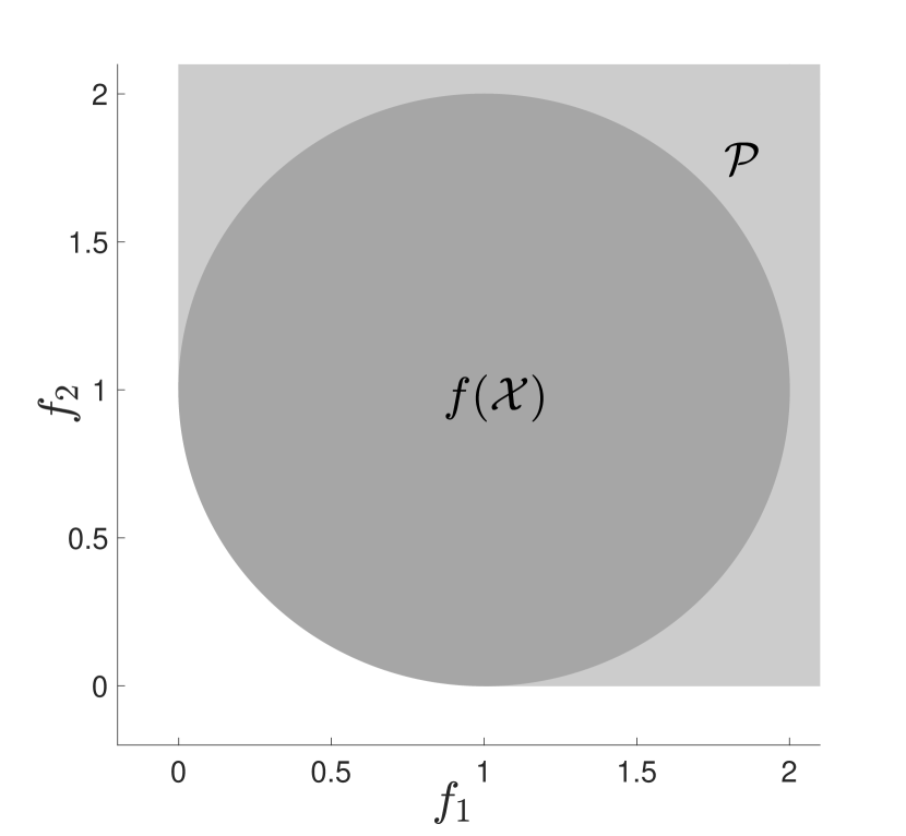
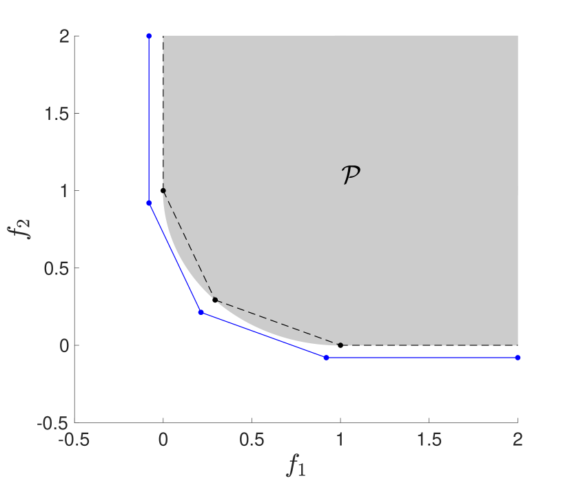
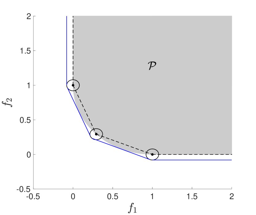
Figure 1: Illustrations of sets $f(\mathcal{X})$, $\mathcal{P}$ (left) and solution concepts given by Definition 3.1 (middle) and Definition 3.2 (right). The dashed lines show ${\rm bd\,}({\rm conv\,}f(\mathcal{\bar{X}})+C)$ (middle and right) and solid blue lines show ${\rm bd\,}({\rm conv\,}f(\mathcal{\bar{X}})+C-\epsilon\{c\})$ (middle) and ${\rm bd\,}({\rm conv\,}f(\mathcal{\bar{X}})+C+B(0,\epsilon))$ (right).

Note that both of these solution concepts yield an outer approximation to the upper image. On the other hand, ${\rm conv\,}f(\bar{\mathcal{X}})+C$ is an inner approximation to $\mathcal{P}$. The Hausdorff distance between these inner and outer sets is bounded [6]. Moreover, as the feasible region $\mathcal{X}$ is compact, for any $\epsilon>0$, there exists a finite weak $\epsilon$-solution (with respect to $c$) to problem (P), see [16, Proposition 4.3] and [2, Proposition 3.8].

There are different solution approaches to solve bounded CVOPs in the sense of Definitions 3.1 or 3.2. The main idea of these approaches is to generate (weak) minimizers for (P) in a structured way. One way of generating (weak) minimizers is to solve scalarization models. Below, we provide two well-known scalarization models together with some results regarding them.

For a weight parameter $w\in\mathbb{R}^{p}$, the weighted sum scalarization model is given by

$$\textrm{minimize }{w^{\mathsf{T}}f(x)}\>\>\textrm{subject to }x\in\mathcal{X}. w$$ (WS())

Proposition 3.3 ([13, Corollary 5.29]).

An optimal solution $x\in\mathcal{X}$ of (WS($w$)) is a weak minimizer of (P) if $w\in C^{+}\setminus\{0\}$. Conversely, for any weak minimizer $x\in\mathcal{X}$, there exists $w\in C^{+}\setminus\{0\}$ such that $x$ is an optimal solution of (WS($w$)).

Pascoletti-Serafini scalarization [20] is given by

$$\textrm{minimize }z\>\>\textrm{subject to }f(x)\leq_{C}v+zd,\>x\in\mathcal{X},\>z\in\mathbb{R}. v,d$$ (PS())

The parameters $v,d\in\mathbb{R}^{p}$ are referred to as the reference point and the direction, respectively. The Lagrange dual of the PS problem can be written as

$$\textrm{maximize }\inf_{x\in\mathcal{X}}w^{\mathsf{T}}f(x)-w^{\mathsf{T}}v\>\>\textrm{subject to }w^{\mathsf{T}}d=1,\>w\in C^{+}, v,d$$ (D-PS())

see [6, 16]. Below, we provide some well-known results regarding (PS($v,d$)) and (D-PS($v,d$)).

Proposition 3.4.

[16, Proposition 4.5] If $(x^{*},z^{*})\in\mathbb{R}^{n+1}$ is an optimal solution of problem (PS($v,d$)), then $x^{*}$ is a weak minimizer. Moreover, $v+z^{*}d\in{\rm bd\,}\mathcal{P}$.

Remark 3.5.

Note that $f(x)\leq_{C}v+zd$ holds for some $x\in\mathcal{X}$ if and only if $v+zd\in\mathcal{P}$. To see, assume $f(x)\leq_{C}v+zd$ holds for some $x\in\mathcal{X}$, that is, $v+zd-f(x)\in C$ holds. Then, we have $v+zd\in\{f(x)\}+C\subseteq f(\mathcal{X})+C=\mathcal{P}$. The other implication follows similarly.

The following propositions show the existence of an optimal solution to problem (PS($v,d$)) under the assumptions of problem (P) together with some additional conditions on the problem parameters. Note that Proposition 3.6 is already stated in [16, Proposition 4.4]. We still provide a proof of it as the one given in [16] has inaccuracies.

Proposition 3.6.

Let $v\in\mathbb{R}^{p}$. If $d\in{\rm int\,}C$, then there exist optimal solutions to (PS($v,d$)) and (D-PS($v,d$)). Moreover, the optimal values of the two problems coincide.

Proof.

First, we show that there exists a feasible solution to (PS($v,d$)). By the assumptions on (P), there exists $\bar{x}\in{\rm int\,}\mathcal{X}$. Let $\bar{z}:=\max_{i\in\{1,\ldots,l\}}\frac{(w^{i})^{\mathsf{T}}(f(\bar{x})-v)}{(w^{i})^{\mathsf{T}}d}+\delta$ for some $\delta>0$, where $C^{+}={\rm co\,}{\rm conv\,}\{w^{1},\ldots,w^{l}\}$. Note that $\bar{z}$ is well defined since $d\in{\rm int\,}C$, hence $(w^{i})^{\mathsf{T}}d>0$ for all $i\in\{1,\ldots,l\}$. It is not difficult to see that $(\bar{x},\bar{z})$ is a feasible solution for (PS($v,d$)). Indeed, $(\bar{x},\bar{z})$ is strictly feasible, hence a Slater point for (PS($v,d$)). Hence, there exists an optimal solution $w^{*}$ for (D-PS($v,d$)) and the optimal values of the two problems coincide.

For the existence of an optimal solution for (PS($v,d$)), we first show that for any feasible solution $(x,z)\in\mathbb{R}^{n+1}$, $z$ is bounded below. As $\mathcal{X}$ is compact, $\eqref{P}$ is bounded, that is, there exists $a\in\mathbb{R}^{p}$ such that $\mathcal{P}\subseteq\{a\}+C$. Then, by Remark 3.5, $v+zd\in\{a\}+C$ holds for any feasible $(x,z)$. This implies that for all $w\in C^{+}$ we have $w^{\mathsf{T}}(v+zd-a)\geq 0$. Since $w^{\mathsf{T}}d>0$ for all $w\in C^{+}\setminus\{0\}$, it is true that

$$z\geq\sup_{w\in C^{+}{\color[rgb]{0,0,0}\setminus\{0\}}}\frac{w^{\mathsf{T}}(a-v)}{w^{\mathsf{T}}d}={\color[rgb]{0,0,0}\sup\left\{\frac{w^{\mathsf{T}}(a-v)}{w^{\mathsf{T}}d}\mid w\in C^{+},\left\|w\right\|=1\right\}}=:\tilde{z}\in\mathbb{R}.$$

Then, without changing the problem, we may add the constraint: $\tilde{z}\leq z\leq\bar{z}$ to (PS($v,d$)). As the feasible region of the equivalent form is compact, (PS($v,d$)) has an optimal solution.∎

Proposition 3.7.

[6, Proposition 3.7] For $v\notin\mathcal{P},y\in{\color[rgb]{0,0,0}}\mathcal{P}$ and $d=y-v$, both (PS($v,d$)) and (D-PS($v,d$)) have optimal solutions and the optimal values coincide.

The next result states that using the primal-dual solution pair to problems (PS($v,d$)) and (D-PS($v,d$)), it is possible to find a supporting hyperplane to the upper image. It will play a critical role in the description of the solution algorithm which will be discussed in Section 4.

Proposition 3.8 ([16, Proposition 4.7]).

Let $v,{\color[rgb]{0,0,0}d}\in\mathbb{R}^{p}$ and $(x^{*},z^{*})$, $w^{*}\in\mathbb{R}^{p}$ be the optimal solutions for (PS($v,d$)) and its Lagrange dual, respectively. If the optimal objective function values of (PS($v,d$)) and (D-PS($v,d$)) coincides, then $H:=\{y\in\mathbb{R}^{p}\mid(w^{*})^{\top}y=(w^{*})^{\mathsf{T}}v+z^{*}\}$ is a supporting hyperplane for $\mathcal{P}$ at $y^{*}=v+z^{*}d$ and $\mathcal{H}=\{y\in\mathbb{R}^{p}\mid(w^{*})^{\mathsf{T}}y\geq(w^{*})^{\mathsf{T}}v+z^{*}\}$ contains $\mathcal{P}$.

Figure 2 illustrates problem (PS($v,d$)) and Proposition 3.8.

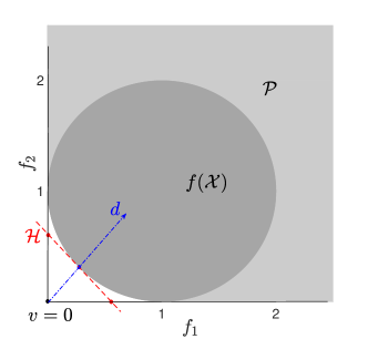
Figure 2: Illustration of (PS($v,d$)) and Proposition 3.8. The blue marker shows the point $v+z^{\ast}d$ and the dashed red line shows the supporting hyperplane $\mathcal{H}$ of $\mathcal{P}$ at $v+z^{\ast}d$.

4 The algorithm and variants

In this section, we will first provide the main framework of a CVOP algorithm that solves PS scalarizations iteratively and finds a finite weak $\epsilon$-solution to problem (P) for a given $\epsilon>0$. Then, we will provide some variants based on selecting the parameters of the scalarizations.

4.1 The algorithm

We consider a CVOP algorithm that starts with an outer approximation to the upper image, iteratively updates it by solving PS scalarizations, and stops when the approximation is fine enough. More specifically, it starts by solving (WS($w^{i}$)) for all $i\in\{1,\ldots,l\}$ where $w^{i}$’s are extreme directions of $C^{+}$. Optimal solutions $x^{i},i\in\{1,\ldots,l\}$ of these problems form the initial set of weak minimizers $\bar{\mathcal{X}}^{0}$. Then, the initial outer approximation $P^{0}$ of $\mathcal{P}$ is set as $P^{0}=\bigcap_{i\in\{1,\ldots,l\}}\mathcal{H}^{i}$ (lines 2, 3 of Algorithm 1), where $\mathcal{H}^{i}=\{y\in{\color[rgb]{0,0,0}\mathbb{R}^{p}}\mid{(w^{i})}^{\mathsf{T}}y\geq{(w^{i})}^{\mathsf{T}}f(x^{i})\}$.

In the $k^{th}$ iteration, the vertices $V^{k}$ of the current outer approximation $P^{k}$ are considered and a vertex that was not used in the previous iterations, i.e., $v\in V^{k}\setminus V_{\textnormal{used}}\,$ is selected. We will later discuss different vertex selection methods, some of which return $V^{k}_{\textnormal{info}}\,\neq\emptyset$. $V^{k}_{\textnormal{info}}\,$ stores triples $(v,y^{v},z^{v})$ for the vertices $v\in V^{k}\setminus V_{\textnormal{used}}\,$, where $y^{v}\in{\rm bd\,}\mathcal{P}$ and $z^{v}=\left\|y^{v}-v\right\|$. In this case, an upper bound for the Hausdorff distance between $P^{k}$ and $\mathcal{P}$, namely $\hat{h}=\max_{v\in V^{k}\setminus V_{\textnormal{used}}\,}z^{v}$ can be computed. If $\hat{h}\leq\epsilon$, the algorithm terminates by letting $V^{k}=\emptyset$. $V^{k}_{\textnormal{info}}\,=\emptyset$ means that the vertex selection method does not store any information regarding the current vertices, see lines 6-12.

If $V^{k}_{\textnormal{info}}\,=\emptyset$ or if the algorithm is not terminated as explained above, then (PS($v,d$)) is solved to find a weak minimizer $x^{v}$, see Proposition 3.4. Note that if the direction parameter $d$ is not fixed from the beginning of the algorithm, then it has to be computed before this step. The selected vertex $v$ is added to $V_{\textnormal{used}}\,$ and the corresponding weak minimizer $x^{v}$ is added to set $\bar{\mathcal{X}}^{k}$ (lines 13-16). If the current vertex is close enough to the upper image, then the algorithm checks another vertex from $V^{k}\setminus V_{\textnormal{used}}\,$. Otherwise, the current outer approximation is updated by intersecting it with the supporting halfspace $\mathcal{H}$ of $\mathcal{P}$ at $f(x^{v})$, see Proposition 3.8. The vertices of the updated outer approximation are computed by solving a vertex enumeration problem (lines 18-20). The algorithm terminates if all the vertices of the current outer approximation are in $\epsilon$ distance to the upper image and returns a set of weak minimizers $\bar{\mathcal{X}}$.

Algorithm 1 Primal Approximation Algorithm for (P)

1:  $V_{\textnormal{used}}\,=\emptyset$, $k=0$, $solve=1$;

2:  For $i=1,\ldots,l$: Solve (WS($w^{i}$)) to find an optimal solution $x^{i}$;

3:  Set $\bar{\mathcal{X}}^{0}=\{x^{1},\ldots,x^{l}\}$ and $P^{0}=\bigcap_{i\in\{1,\ldots,l\}}\{y\in{\color[rgb]{0,0,0}\mathbb{R}^{p}}\mid(w^{i})^{\mathsf{T}}y\geq(w^{i})^{\mathsf{T}}f(x^{i})\}$;

4:  Compute the set of vertices $V^{0}$ of $P^{0}$;

5:  Fix rules for selecting a vertex from $V^{k}$ and a direction parameter $d$;

6:  while $V^{k}\setminus V_{\textnormal{used}}\,\neq\emptyset$ do

7:     $[v,V^{k}_{\textnormal{info}}\,]\leftarrow$SelectVertex($V^{k},V_{\textnormal{used}}\,$);

8:     if $V^{k}_{\textnormal{info}}\,\neq\emptyset$ then

9:        if $\hat{h}=\max_{v\in V^{k}\setminus V_{\textnormal{used}}\,}z^{v}\leq\epsilon$ then

10:           $V^{k}=\emptyset$, $solve=0$;

11:        end if

12:     end if

13:     if $V^{k}_{\textnormal{info}}\,=\emptyset$ or $solve=1$ then

14:        (If not fixed) compute $d^{v}$ such that $d^{v}\in{\rm int\,}C$ and $\left\|d^{v}\right\|=1$;

15:        Solve (PS($v,d^{v}$))/(D-PS($v,d^{v}$)). Let $(x^{v},z^{v})$ and $w^{v}$ be optimal solutions;

16:        $V_{\textnormal{used}}\,\leftarrow V_{\textnormal{used}}\,\cup\{v\}$, $\bar{\mathcal{X}}^{k}\leftarrow\bar{\mathcal{X}}^{k}\cup\{x^{v}\}$;

17:        if $z^{v}>\epsilon$ then

18:           Compute $\mathcal{H}=\{y\in\mathbb{R}^{p}\mid(w^{v})^{\mathsf{T}}y\geq(w^{v})^{\mathsf{T}}v+z^{v}\}$;

19:           $P^{k+1}\leftarrow P^{k}\cap\mathcal{H}$, $\bar{\mathcal{X}}^{k+1}\leftarrow\bar{\mathcal{X}}^{k}$;

20:           Compute the set of vertices $V^{k+1}$ of $P^{k+1}$;

21:           $k\leftarrow k+1$;

22:        end if

23:     end if

24:  end while

25:  return  $\bar{\mathcal{X}}^{k}$

Remark 4.1.

In Algorithm 1, to obtain a coarser set of solutions, instead of adding all weak minimizers to the solution set, one can add the ones which satisfy $z^{v}\leq\epsilon$.

Later, we will discuss different rules for selecting the direction parameter and the vertices, respectively in Sections 4.2 and 4.3. The following proposition holds for any selection rule.

Proposition 4.2.

When terminates, Algorithm 1 returns a finite weak $\epsilon$-solution.

Proof.

There exists optimal solutions $x^{i}$ to (WS($w^{i}$)) for all $i\in\{1,\ldots,l\}$ as $\mathcal{X}$ is compact and $f$ is continuous. Moreover, $\mathcal{H}^{i}=\{y\in\mathbb{R}^{p}\mid(w^{i})^{\mathsf{T}}y\geq(w^{i})^{\mathsf{T}}f(x^{i})\}\supseteq\mathcal{P}=f(\mathcal{X})+C$ holds since $x^{i}$ is an optimal solution for (WS($w^{i}$)) and $\inf_{c\in C}(w^{i})^{\mathsf{T}}c=0$. Then, $P^{0}\supseteq\mathcal{P}$. Moreover, $P^{0}$ has at least one vertex as $C$ is pointed and (P) is bounded, see [21, Corollary 18.5.3]. Hence, we have $V^{0}\neq\emptyset$ (consequently $V^{0}\setminus V_{\textnormal{used}}\,\neq\emptyset$). By Proposition 3.3, the initial solution set $\bar{\mathcal{X}}^{0}=\{x^{1},\ldots,x^{l}\}$ consists of weak minimizers. See lines 2-4 of Algorithm 1.

At iteration $k$, SelectVertex() returns a vertex $v\in V^{k}\setminus V_{\textnormal{used}}\,$ and $V^{k}_{\textnormal{info}}\,$. First, consider the case $V^{k}_{\textnormal{info}}\,=\emptyset$. As $d^{v}\in{\rm int\,}C$ is ensured (line 14), by Proposition 3.6, there exists solutions $(x^{v},z^{v})$ and $w^{v}$ to (PS($v,d^{v}$)) and (D-PS$(v,d^{v})$), respectively. By Proposition 3.4, $x^{v}$ is a weak minimizer. Hence, for any iteration $k$, $\bar{\mathcal{X}}^{k}$ is finite and contains only the weak minimizers (line 16). By Proposition 3.8, $\mathcal{H}=\{y\in\mathbb{R}^{p}\mid(w^{v})^{\mathsf{T}}y\geq(w^{v})^{\mathsf{T}}v+z^{v}\}\supseteq\mathcal{P}$ (line 18). Since $P^{0}\supseteq\mathcal{P}$ and $P^{k+1}=P^{k}\cap\mathcal{H}$ for all $k\geq 0$, we have $P^{k}\supseteq\mathcal{P}$ for all $k\geq 0$ through the algorithm.

The algorithm terminates when $V^{k}\setminus V_{\textnormal{used}}\,=\emptyset$. Assume this is the case after $K$ iterations. This suggests that each $v\in V^{K}$ is also an element of $V_{\textnormal{used}}\,$, that is, $V^{K}\subseteq V_{\textnormal{used}}\,$ (line 16) and $z^{v}\leq\epsilon$ for all $v\in V^{K}$ at termination (line 17). To show that $\bar{\mathcal{X}}^{K}$ is a finite weak $\epsilon$-solution of (P) in the sense of Definition 3.2, it is sufficient to have

$$P^{K}\subseteq{\rm conv\,}f(\bar{\mathcal{X}}^{K})+C+B(0,\epsilon).$$ (1)

Similar to [2, Lemma 5.2], one can show that the recession cone of $P^{k}$ is $C$ for any $k$. Hence, $P^{K}={\rm conv\,}V^{K}+C$ holds true. Then, for any $p\in{\color[rgb]{0,0,0}P^{K}}$, there exist $(\lambda^{v})_{v\in V^{K}}\geq 0$ and $\bar{c}\in C$ such that $\sum_{v\in V^{K}}\lambda^{v}=1$ and $p=\sum_{v\in V^{K}}\lambda^{v}v+\bar{c}$. On the other hand, for each $v\in V^{K}\subseteq V_{\textnormal{used}}\,$, there exist $x^{v}\in\bar{\mathcal{X}}^{K}$, $z^{v}\leq\epsilon$ such that $(x^{v},z^{v})$ is an optimal solution of (PS($v,d^{v}$)). In particular, there exists $c^{v}\in C$ such that $v+d^{v}z^{v}=f(x^{v})+c^{v}$. These imply

$$p=\sum_{v\in V^{K}}\lambda^{v}v+\bar{c}= \sum_{v\in V^{K}}\lambda^{v}(f(x^{v})+c^{v}-d^{v}z^{v})+\bar{c}$$

$$= \sum_{v\in V^{K}}\lambda^{v}f(x^{v})+\sum_{v\in V^{K}}\lambda^{v}c^{v}+\bar{c}-\sum_{v\in V^{K}}\lambda^{v}d^{v}z^{v}{\color[rgb]{0,0,0}.}$$

Clearly, $\sum_{v\in V^{k}}\lambda^{v}f(x^{v})\in{\rm conv\,}f(\mathcal{\bar{X}}^{K})$ and $\sum_{v\in V^{K}}\lambda^{v}c^{v}+\bar{c}\in C$. Moreover, as $z^{v}\leq\epsilon$ and $\left\|d^{v}\right\|=1$ for each $v\in V^{K}$, we have $\sum_{v\in V^{K}}\lambda^{v}z^{v}d^{v}\in B(0,\epsilon)$. Hence, $p\in{\rm conv\,}f(\bar{\mathcal{X}}^{K})+C+B(0,\epsilon)$ and this implies (1) as $p\in{\color[rgb]{0,0,0}P^{K}}$ is arbitrary.

For the vertex selection rules that give $V^{k}_{\textnormal{info}}\,\neq\emptyset$, assume $\hat{h}=\max_{v\in V^{K}\setminus V_{\textnormal{used}}\,}z^{v}\leq\epsilon$ holds for some $K$. Note that if there exists a vertex $v$ in $V^{K}\cap V_{\textnormal{used}}\,$, then $z^{v}\leq\epsilon$ has to be satisfied by the structure of the algorithm. Hence, for the vertices $V^{K}$ of $P^{K}$, we have $z^{v}\leq\epsilon$. Similar steps for the previous case can be applied to show that $\bar{\mathcal{X}}^{K}$ is a finite weak $\epsilon$-solution of (P). ∎

4.2 Direction selection rules

As explained in Section 1, algorithms from [16] and [7] follow the framework given by Algorithm 1. In [16], a fixed direction parameter $d$ is used within (PS($v,d$)) and in [7], $d^{v}$ is taken as $\hat{p}-v$ for a fixed point $\hat{p}\in\mathcal{P}$. Before proceeding with the proposed direction selection rules, we use two examples (Examples 1 (for $p=2$) and 2 provided in Section 5.1) to show that the selection of $d$ in [16] and $\hat{p}$ in [7] affect the performance of these algorithms significantly. The results are summarized in Table 2, in which we report the number of scalarization models (SC) and the CPU time (T).

Table 2: Results for different $d$ and $\hat{p}$ values fixed for algorithms in [16] and [7], respectively

	Example 1 ($p=2,\epsilon=0.005)$								Example 2 ($\epsilon=0.05)$
	$d$ in [16]				$\hat{p}$ in [7]				$d$ in [16]			$\hat{p}$ in [7]
	$\begin{pmatrix}1\\ 1\end{pmatrix}$	$\begin{pmatrix}0.1\\ 1\end{pmatrix}$	$\begin{pmatrix}0.01\\ 1\end{pmatrix}$	$\begin{pmatrix}0.001\\ 1\end{pmatrix}$	$\begin{pmatrix}1\\ 1\end{pmatrix}$	$\begin{pmatrix}0.1\\ 1\end{pmatrix}$	$\begin{pmatrix}0.01\\ 1\end{pmatrix}$	$\begin{pmatrix}0.001\\ 1\end{pmatrix}$	$\begin{pmatrix}1\\ 1\end{pmatrix}$	$\begin{pmatrix}0.1\\ 1\end{pmatrix}$	$\begin{pmatrix}0.01\\ 1\end{pmatrix}$	$\begin{pmatrix}100\\ 100\end{pmatrix}$	$\begin{pmatrix}10\\ 1000\end{pmatrix}$	$\begin{pmatrix}10\\ 10000\end{pmatrix}$
SC	29	27	35	41	17	31	39	47	31	56	304	30	178	741
T	10.10	9.94	13.34	14.62	6.27	11.06	13.97	23.76	13.60	18.19	93.81	10.52	61.12	226.63

Motivated by these results, we propose two additional selection rules for the direction parameter to be used in PS scalarization.

Adjacent vertices-based approach (Adj).

When the double description method is used to solve the vertex enumeration problem (line 20 of Algorithm 1), the sets of adjacent vertices for each vertex are also returned. We use this information to compute the direction parameter for a given vertex. In particular, for each vertex $v$, the normal direction of a hyperplane passing through the adjacent vertices of $v$ is computed. The main motivation for this selection rule is that the positions of the adjacent vertices depend on the curvature of the upper image as they are formed by the supporting hyperplanes of the upper image at points that are possibly close to the current vertex. This geometric intuition is illustrated in Figure 3 for a two-dimensional setting.

Note that the adjacency list of a vertex may also contain extreme directions. If for a vertex $v$, we have an adjacent extreme direction $z$, then it is known that the line segment $\{v+rz\in\mathbb{R}^{p}\mid r\geq 0\}$ is a face of $P^{k}$. In these cases, we construct an artificial adjacent vertex by moving the current vertex along the adjacent extreme direction, that is, we take $v+z$. An example of this case can be seen in Figure 3.

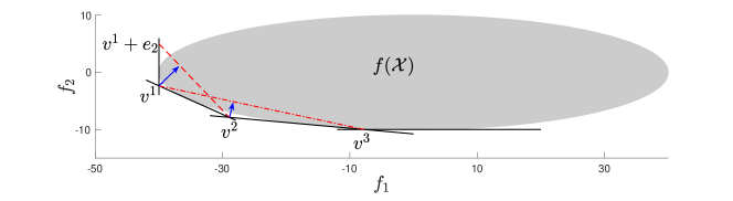
Figure 3: Three vertices of the current outer approximation are $v^{1},v^{2}$ and $v^{3}$. The adjacent vertices of $v^{1}$ ($v^{2}$ and $v^{1}+e_{2}$) and $v^{2}$ ($v^{1}$ and $v^{3}$) and the directions based on the Adjacent vertices approach from vertices $v^{1}$ and $v^{2}$ are illustrated.

In general, a vertex may have more adjacent vertices than required. In that case, we choose $p$ of the vertices, $v^{i_{1}}_{adj},\ldots,\ v^{i_{p}}_{adj}$ and compute $d\in\mathbb{R}^{p}$ such that $d^{\mathsf{T}}v^{i_{1}}_{adj}=\ldots=d^{\mathsf{T}}v^{i_{p}}_{adj}$, see line 3 of Procedure 2. Note that it is possible to obtain $-d$ as the solution of this system. On the other hand, by Proposition 3.6, if $d\in{\rm int\,}C$ we obtain a weak minimizer by solving (PS($v,d$)). Hence, we first check if one of two candidate unit normal vectors, $d$ or $-d$, is in ${\rm int\,}C$. If this is not the case, we use a predetermined direction $d\in{\rm int\,}C$ where $\left\|d\right\|=1$. In particular, we set $d=\frac{\sum_{i=1}^{r}c^{i}}{\left\|\sum_{i=1}^{r}c^{i}\right\|}$, where $c^{1},\ldots,c^{r}$ are the extreme directions of $C$.

Procedure 2 ChooseDirection($v$,$P$)

1:  Let $v^{1}_{adj},v^{2}_{adj},\ldots,\ v^{s}_{adj}$ be the vertices adjacent to $v$;

2:  Pick $p$ vertices $v^{i_{1}}_{adj},\ldots,\ v^{i_{p}}_{adj}$ and let $A=[v^{i_{1}}_{adj},\ldots,\ v^{i_{p}}_{adj}]\in\mathbb{R}^{p\times p}$;

3:  Compute $d\in B(0,1)$ satisfying $A^{\mathsf{T}}d=e$ ($d=\frac{A^{-\mathsf{T}}e}{\left\|A^{-\mathsf{T}}e\right\|}$ if $A^{-1}$ exists.);

4:  if $d\in{\rm int\,}C$ then

5:     return  $d$

6:  else if $-d\in{\rm int\,}C$ then

7:     return  $-d$

8:  else

9:     return  $d=\frac{\sum_{i=1}^{r}c^{i}}{\left\|\sum_{i=1}^{r}c^{i}\right\|}$, where $c^{1},\ldots,c^{r}$ are the extreme directions of $C$.

10:  end if

Remark 4.3.

For $p=2,C=\mathbb{R}^{2}_{+}$, it is easy to show that either $d\in{\rm int\,}C$ or $-d\in{\rm int\,}C$ is satisfied (see Figure 3 for an illustration). However, this may not be true in general for $p\geq 3$ or for $C\neq\mathbb{R}^{2}_{+}$. Through our computational tests, we obtain some counterexamples for $p=4$. Even though we haven’t encountered this situation for $p=3$, it is still possible that $\pm d\notin{\rm int\,}\mathbb{R}^{3}_{+}$. See Figure 4 for an illustration, in which vertex $v=0\in\mathbb{R}^{3}$ has 4 adjacent vertices: $v^{1}_{adj}=(-1,1,1)^{\mathsf{T}},\>v^{2}_{adj}=(1,1,-1)^{\mathsf{T}},\>v^{3}_{adj}=(3.3,-2.2,-1.1)^{\mathsf{T}},\>v^{4}_{adj}=(5,-4,1)^{\mathsf{T}}$. (Note that $v,v^{1}_{adj},\ldots,v^{4}_{adj}$ are still extreme points of the set ${\rm conv\,}\{v,v^{1}_{adj},\ldots,v^{4}_{adj}\}+\mathbb{R}^{3}_{+}$. For illustrative purposes, the figure shows ${\rm conv\,}\{v,v^{1}_{adj},\ldots,v^{4}_{adj}\}$.) The normal direction $d$ of the hyperplane passing through $v^{2}_{adj},v^{3}_{adj},v^{4}_{adj}$ satisfies $d\notin{\rm int\,}\mathbb{R}^{3}_{+}$ and $-d\notin{\rm int\,}\mathbb{R}^{3}_{+}$.

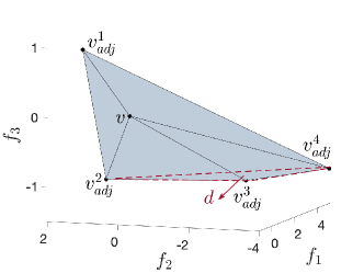
Figure 4: An example with $p=3,C=\mathbb{R}^{3}_{+}$ for which $d$ computed in line 5 of Procedure 2 is not in $\pm{\rm int\,}\mathbb{R}^{3}_{+}$. In particular, the normal direction of the hyperplane passing thorough $v^{2}_{adj},v^{3}_{adj},v^{4}_{adj}$ is $d=(0.2273,0.1818,-0.5909)^{\mathsf{T}}$.

Ideal point-based approach (IP).

For this approach, we assume that the ordering cone is $\mathbb{R}^{p}_{+}$, hence the ideal point $y^{I}$ is well defined. For a vertex $v$ of the current outer approximation, we consider the vector $v-y^{I}$. Note that for the initial iteration, we have $v-y^{I}=0$. In the subsequent iterations, we obtain $v-y^{I}\geq 0$ since $P^{k}\subseteq P^{0}$ for any $k$ throughout the algorithm. For $i\in\{1,\ldots,p\}$, we define $d_{i}=\frac{1}{v_{i}-y^{I}_{i}+\bar{\epsilon}}$ for some sufficiently small $\bar{\epsilon}>0$, which is added for computational convenience. For the numerical examples, we take $\bar{\epsilon}=10^{-5}$. Then $d$ is normalized such that $\left\|d\right\|=1$. Geometrically, this corresponds to considering the points $(v_{i}-y^{I}_{i})e_{i}$ for each $i\in\{1,\ldots,p\}$ and taking the normal direction of the hyperplane passing through them.

4.3 Vertex selection rules

We propose different vertex selection rules that can be used within Algorithm 1. As will be detailed in Section 4.4, there are algorithms from the literature using some vertex selection rules that require solving additional optimization models, see [6, 14]. Our motivation is to propose vertex selection rules which are computationally less complicated yet have the potential to increase the efficiency of Algorithm 1.

Vertex selection with clusters (C).

This vertex selection rule clusters the vertices of the current outer approximation and visits these clusters sequentially. The motivation is to ensure that the vertices from different regions of the outer approximation are selected in a balanced fashion.

The first step is to fix centers for the clusters, which can be done in different ways. For this purpose, we first solve (PS($v,d$)) for each vertex of the initial polyhedron $P^{0}$. The corresponding supporting halfspaces are intersected with the current polyhedron to obtain $P^{1}$. The same procedure is repeated for $P^{1}$ and the vertices of $P^{2}$ are selected as the centers of the clusters, see Procedure 3. It is possible to use the vertices of $P^{1}$ to have fewer clusters or continue in the same fashion and use the vertices of $P^{k}$ for some $k>2$ to have more clusters. Note that SelectCenters($V^{0}$,$P^{0}$) has to be called right before line 6 of Algorithm 1.

Procedure 3 SelectCenters($V^{0}$,$P^{0}$)

1:  for $k\in\{0,1\}$ do

2:     for all $v\in V^{k}$ do

3:        Solve (PS($v,d$)), let $(x^{v},z^{v})$ be the optimal solution, $\bar{\mathcal{X}}\leftarrow\bar{\mathcal{X}}\cup\{x^{v}\}$;

4:        Find supporting halfspace $\mathcal{H}$ of $\mathcal{P}$ at $y^{v}=v+z^{v}d$, $P^{k+1}\leftarrow P^{k}\cap\mathcal{H}$;

5:     end for

6:     Compute the set of vertices $V^{k+1}$ of $P^{k+1}$;

7:  end for

8:  $\mathcal{C}=\emptyset$.

9:  for $v\in V^{2}$ do

10:     $\mathcal{C}\leftarrow\mathcal{C}\cup\{v\}$;

11:  end for

12:  return  $\mathcal{C}$

For the remaining iterations of Algorithm 1, each vertex of the current outer approximation is assigned to the cluster whose center is the closest with respect to the Euclidean distance. Whenever a vertex has to be selected, a vertex is chosen arbitrarily from the cluster in turn. If there is no unexplored vertex assigned to the current cluster, then the algorithm selects the next nonempty cluster. The pseudocode is given in Procedure 4.

Procedure 4 SelectVertex($t,V^{k},V_{\textnormal{used}}\,,\mathcal{C}$)

1:  Initialize the $i^{th}$ cluster with center $c_{i}\in\mathcal{C}$ as $\mathcal{C}_{i}=\emptyset$ for $i\in\{1,\ldots,|\mathcal{C}|\}$;

2:  for all $v\in V^{k}\setminus V_{\textnormal{used}}\,$ do

3:     Pick $i\in\operatorname*{arg\,min}_{i\in\{1,\cdots,|\mathcal{C}|\}}\left\|v-c_{i}\right\|$ and $\mathcal{C}_{i}\leftarrow\mathcal{C}_{i}\cup\{v\}$;

4:  end for

5:  $\textnormal{current}\equiv t+1\pmod{|\mathcal{C}|}$;

6:  while $\mathcal{C}_{\textnormal{current}}=\emptyset$ do

7:     $t\leftarrow t+1$ and $\textnormal{current}\leftarrow t+1\pmod{|\mathcal{C}|}$;

8:  end while

9:  Pick an arbitrary $v\in\mathcal{C}_{\textnormal{current}}$;

10:  $t\leftarrow t+1$;

11:  return  $v$, $t$

Vertex selection with adjacency information (Adj).

Recall that bensolve tools returns the adjacency information for the vertices of the outer approximation. We use this to detect “isolated” vertices of the current outer approximation. The motivation is to obtain uniformity among the vertices of the outer approximation and consequently, the $C$-minimal points found on the boundary of the upper image as long as the geometry allows. For each vertex $v$, the procedure finds the minimum distance, say $dist_{v}$, from $v$ to its current neighbors. Then, it selects the vertex which has the maximum $dist_{v}$, see Procedure 5.

Procedure 5 SelectVertex($V^{k}$,$V_{\textnormal{used}}\,$)

1:  for all $v\in V^{k}\setminus V_{\textnormal{used}}\,$ do

2:     Let ${\color[rgb]{0,0,0}V^{v}_{adj}}$ be the set of vertices adjacent to $v$;

3:     Let $dist_{v}=\min_{\tilde{v}\in{\color[rgb]{0,0,0}V^{v}_{adj}}}\left\|\tilde{v}-v\right\|$;

4:  end for

5:  return  $v^{*}\in\operatorname*{arg\,max}_{v\in V^{k}\setminus V_{\textnormal{used}}\,}dist_{v}$.

Vertex selection using local upper bounds (UB).

This selection rule can only be used for $C=\mathbb{R}^{p}_{+}$. It is motivated by split algorithms, which are originally designed to solve multiobjective integer programming problems, see for instance [5, 12, 3]. The main idea is to find a set of local upper bounds for the nondominated points and use them to select a vertex.

For this method, in line 1 of Algorithm 1, we additionally fix an upper bound $u=Me$ where $M$ is a sufficiently large number such that $\{u\}-\mathbb{R}^{p}_{+}\supseteq f(\mathcal{X})$ and we initialize the set of upper bounds as $U=\{(u,\emptyset)\}$. Here, $\emptyset$ means that the upper bound $u$ is not defined based on any other (weakly) nondominated point found in the algorithm. Note that the initial upper bound $u$ satisfies that $y^{I}\leq u$. Through the algorithm, for any vertex $v$ of $P^{k}$, it is guaranteed that there exists a local upper bound $u$ such that $v\leq u$. Indeed, among all the upper bounds satisfying $v\leq u$, we fix the one that yields the minimum $\left\|v-u\right\|$ value as the ‘corresponding’ local upper bound for $v$.

Together with the vertex $v$ to proceed, this method returns also the corresponding local upper bound $u$ where $(u,y)\in U$. Let $(x^{v},z^{v})$ be an optimal solution for (PS($v,d$)). Using ${\color[rgb]{0,0,0}y^{v}}:=v+z^{v}d\in{\rm bd\,}\mathcal{P}$, $p$ new upper bounds $u^{1},\ldots,u^{p}$ are generated as follows: for $j\in\{1,\ldots,p\}$, we set $u^{j}_{i}=u_{i}$ for each $i\in\{1,\ldots,p\}\setminus\{j\}$ and $u^{j}_{j}=y_{j}^{v}$. Then, the list of upper bounds is updated accordingly. To capture these changes, line 7 of Algorithm 1 is replaced by

$$[v,(u,y),V^{k}_{\textnormal{info}}\,]\leftarrow\textnormal{SelectVertex}(U,V^{k},V_{\textnormal{used}}\,);$$

and line 15 of Algorithm 1 is modified as in Procedure 6.

Procedure 6 Line 15 of Algorithm 1 for UB

  Solve (PS($v,d$))/(D-PS($v,d$)). Let $(x^{v},z^{v})$/$w^{v}$ be optimal solutions and $y^{v}=v+z^{v}d$;

  for $j=1:p$ do

     $u^{j}\leftarrow u$, $u^{j}_{j}\leftarrow y^{v}_{j}$, $U\leftarrow U\cup\{(u^{j},y^{v})\}$;

  end for

  $U\leftarrow U\setminus\{(u,y)\}$;

For the vertex selection procedure, we first assign the corresponding upper bounds for each vertex (line 3 of Procedure 7). Then, we choose $v^{\ast}\in V^{k}\setminus V_{\textnormal{used}}\,$, which has the greatest distance to its corresponding local upper bound $u^{\ast}$ (lines 10 and 12 of Procedure 7). Note that $\left\|v^{*}-u^{*}\right\|$ yields an upper bound for the current approximation error since we have $d_{H}(P^{k},\mathcal{P})=\max_{v\in V^{k}}d(v,\mathcal{P})\leq\max_{v\in V^{k}}\left\|v-u^{v}\right\|=\left\|v^{*}-u^{*}\right\|,$ where $u^{v}$ denotes the corresponding upper bound of $v$. As it will be detailed in Section 4.4, the algorithms proposed in [14] and [6] also compute an upper bound for the approximation error during any iteration. Different from them, UB does not solve optimization models to find this approximation error.

Note that some upper bounds have components equal to $M$. This causes the distances between $v$ and its corresponding upper bound to be significantly large. To tackle this, the modifications are made, see lines 4-9 of Procedure 7 for the details.

Procedure 7 SelectVertex($U$,$V^{k},V_{\textnormal{used}}\,$)

1:  $V^{k}_{\textnormal{info}}\,=\emptyset$

2:  for all $v\in V^{k}\setminus V_{\textnormal{used}}\,$ do

3:     Let $(\hat{u},\hat{y})\in\operatorname*{arg\,min}_{\{(u,y)\in U\colon v\leq u\}}\left\|v-u\right\|$;

4:     $u^{\textnormal{temp}}=\hat{u}$;

5:     for $i=1\colon p$ do

6:        if $\hat{u}_{i}=M$ then

7:           $u^{\textnormal{temp}}_{i}\leftarrow\max\{\textnormal{avg},\hat{y}_{i}\}$;

8:        end if

9:     end for

10:     $\hat{z}=\left\|v-u^{\textnormal{temp}}\right\|,V^{k}_{\textnormal{info}}\,\leftarrow V^{k}_{\textnormal{info}}\,\cup\{(v,\hat{u},\hat{z})\}$;

11:  end for

12:  Let $(v^{\ast},u^{\ast},z^{\ast})\in\operatorname*{arg\,max}_{(v,u,z)\in V^{k}_{\textnormal{info}}\,}z$, and let $y^{\ast}$ be such that $(u^{\ast},y^{\ast})\in U$;

13:  return  $v^{\ast},(u^{\ast},y^{\ast}),V^{k}_{\textnormal{info}}\,$

Remark 4.4.

For Procedure 7 to work correctly, we modify Algorithm 1 slightly as follows: In line 1, we initialize $V^{0}_{\textnormal{info}}$ as an empty set and in line 19 we also update $V^{k+1}_{\textnormal{info}}\leftarrow V^{k}_{\textnormal{info}}\,$. The same modification is also applied to the algorithms from the literature that will be explained in Section 4.4.

4.4 Algorithms from the literature

In this section, we briefly explain similar approaches from the literature, namely, Algorithm KTW from [14], Algorithm DLSW from [6], and an algorithm from [2]. The algorithm from [2] does not totally fit into the framework of Algorithm 1 as it solves a different scalarization model in each iteration. Here, we consider a variant of Algorithm 1, which is motivated by the one from [2].

Algorithm KTW.

The outer approximation algorithm provided in [14] is a special case of the general framework given by Algorithm 1, applied to a maximization problem. Here, we shortly explain it for problem (P). KTW assumes $0\in\mathcal{P}$. In iteration $k$, it minimizes the distance (with respect to an oblique norm) between the current outer approximation and the upper image. To do that, for every vertex $v\in V^{k}\setminus V_{\textnormal{used}}\,$, it solves:

$$\textrm{maximize }\lambda\>\>\textrm{subject to }f(x)\leq\lambda v,\>x\in\mathcal{X},\>\lambda\in\mathbb{R}.$$ (2)

Assuming $(x^{v},\lambda^{v})$ is an optimal solution to (2), $v^{*}\in\operatorname*{arg\,min}_{v\in V^{k}\setminus V_{\textnormal{used}}\,}\lambda^{v}$ is selected in Algorithm 1.

Problem (2) is equivalent to (PS($v,d$)) with $d=-v$. Indeed, $(x^{v},\lambda)$ is an optimal solution to (2) if and only if $(x^{v},1-\lambda)$ is an optimal solution to (PS($v,-v$)). Note that KTW is similar to the algorithm proposed in [7] in the sense that $\hat{p}=0$ is fixed. However, different from [7], the selection of the vertices in each iteration is not arbitrary in KTW.

For the examples from Section 5.1, it is not guaranteed that $0\in\mathcal{P}$. To overcome this, for the computational tests that will be presented in Section 6, we take $\hat{p}$ as in (6). Then, we modify the model given in (2) as:

$$\textrm{maximize }\lambda\>\>\textrm{subject to }f(x)\leq\hat{p}+\lambda(v-\hat{p}),\>x\in\mathcal{X},\>\lambda\in\mathbb{R}.$$ (3)

This simply corresponds to shifting the upper image as well as the vertices of the outer approximation by $\hat{p}\in\mathcal{P}$. To have a more efficient implementation to select the vertices, we do not solve (7) for all $v\in V^{k}\setminus V_{\textnormal{used}}\,$. Instead, we check if (7) is solved in previous iterations.

Algorithm DLSW.

Dörfler et al. [6] propose a vertex selection rule that uses the inner approximation obtained in each iteration. Accordingly, for each vertex $v$ of the current outer approximation $P^{k}$, the following problem, which measures the distance from $v$ to the current inner approximation $\mathcal{I}^{k}:={\rm cl\,}{\rm conv\,}f(\bar{\mathcal{X}}^{k})+C$, is solved:

$$\textrm{minimize }\left\|y-v\right\|^{2}\>\>\textrm{subject to }y\in\mathcal{I}^{k}.$$ (4)

Then, vertex $v^{\ast}$ which is the farthest away from the inner approximation is selected, that is, $v^{\ast}\in\operatorname*{arg\,max}_{v\in V^{k}\setminus V_{\textnormal{used}}\,}\left\|y^{v}-v\right\|$, where $y^{v}$ is an optimal solution of (8). Moreover, $d$ is set to $\frac{y^{v^{\ast}}-v^{\ast}}{\left\|y^{v^{\ast}}-v^{\ast}\right\|}$. An upper bound for the Hausdorff distance between the current outer approximation and the upper image is found as $\left\|y^{v^{\ast}}-v^{\ast}\right\|$.

In [6], also an improved version of this algorithm is presented. Using the information from the previous iterations, it is possible to skip solving (8) for some of the vertices. In particular, for $x^{k}$ being the weak minimizer found in iteration $k$, if (8) is solved for some $v$ in the previous iterations and $(y^{v}-v)^{\mathsf{T}}(f(x^{k})-y^{v})\geq 0$ holds true, then the solution of (8) for $v$ in iterations $k$ and $k-1$ are the same by [6, Theorem 4.4]. Hence there is no need to solve (8) for $v$. See [6] for the details.

Algorithm AUU.

Ararat et al. [2] propose an outer approximation algorithm to solve CVOPs. Even though this algorithm is similar to Algorithm 1, it is different since instead of (PS($v,d$)), it solves the following scalarization:

$$\textrm{minimize }\left\|z\right\|\>\>\textrm{subject to }f(x)\leq_{C}v+z,\>x\in\mathcal{X},z\in\mathbb{R}^{p}.$$ (5)

Note that (9) does not require a direction parameter. Instead, it computes the distance $z^{v}$ from $v$ to the upper image, where $(x^{v},z^{v})$ is an optimal solution. If one solves (9) for all vertices of the current outer approximation $P^{k}$, then it is possible to compute the exact Hausdorff distance between $P^{k}$ and $\mathcal{P}$ as $\max_{v\in V^{k}}z^{v}$, where $V^{k}$ is the set of vertices of $P^{k}$. See [2] for the details.

As the main motivation of this study is to compare the effect of parameter selection rules for the PS scalarization, we consider a variant (namely, Algorithm AUU) of Algorithm 1 which is motivated by the algorithm from [2]. For AUU, we solve (9) only for parameter selection for the PS scalarizations and we still execute line 14 of Algorithm 1. The direction parameter is set as $d=\frac{z^{v}}{\left\|z^{v}\right\|}$. Note that this is the direction that would yield the minimum optimal objective function value for (PS($v,d$)).

In [2], the vertex selection is arbitrary, however, a special vertex selection rule is discussed in [2, Corollary 7.4 and Remark 7.5] to obtain a convergence result. Here, for algorithm AUU, we apply this vertex selection rule, that is, we solve (9) for each vertex of $P^{k}$ and select the one that is the farthest away from the upper image. This allows the algorithm to provide the approximation error in each iteration rather than at termination. Indeed, by Lemma 2.2, this approximation error is equal to the Hausdorff distance between $\mathcal{P}$ and the outer approximation. As in KTW, the solution of (9) for a vertex $v$ is added to $V^{k}_{\textnormal{info}}\,$, if (9) is not solved for $v$ in the previous iterations.

5 Test examples and preliminary results

Before we proceed with the main computational study, we provide the numerical examples that will be used throughout. Moreover, to possibly decrease the number of variants to be tested for the main computational study, we provide some preliminary results.

For the computational tests provided here and in Section 6, the algorithms are implemented using MATLAB R2020b. The scalarizations are solved via CVX v2.2 [10, 9] and SeDuMi 1.3.4 [23]. Vertex enumeration problems are solved by bensolve tools [18], which is a free solver providing commands for the calculus of convex polyhedra and polyhedral convex functions for Octave and MATLAB. The computer specification that is used throughout the computational study is Intel(R) Core(TM) i7-4790 CPU @ 3.60GHz.

5.1 Test examples

Consider problem (P), where the ordering cone $C$ is $\mathbb{R}^{p}_{+}$; and objective function $f:\mathbb{R}^{n}\to\mathbb{R}^{p}$ and feasible region $\mathcal{X}\subseteq\mathbb{R}^{n}$ are given as follows:

1. Example 1. $f(x)=x,\>\mathcal{X}=\{x\in\mathbb{R}^{n}\mid\left\|x-e\right\|\leq 1,\>x\geq 0\}$ for $n=p\in\{{\color[rgb]{0,0,0}2,}3,4\}$.

2. Example 2. $f(x)=\left(x,\>\frac{1}{x}\right)^{\mathsf{T}},\>\mathcal{X}=\mathbb{R}_{+}$.

3. Example 3. Four instances of the following example are considered for $a\in\{5,7,10,20\}$:

   $$f(x)=x,\>\mathcal{X}=\left\{x\in\mathbb{R}^{3}\big{|}\left(\frac{x_{1}-1}{1}\right)^{2}+\left(\frac{x_{2}-1}{a}\right)^{2}+\left(\frac{x_{3}-1}{5}\right)^{2}\leq 1\right\}.$$

4. Example 4. Three instances of the following example are considered for $a\in\{5,7,10\}$:

   $$f(x)=x,\>\mathcal{X}=\left\{x\in\mathbb{R}^{4}\big{|}\left(\frac{x_{1}-1}{1}\right)^{2}+\left(\frac{x_{2}-1}{a}\right)^{2}+\left(\frac{x_{3}-1}{5}\right)^{2}+\left(\frac{x_{4}-1}{1}\right)^{2}\leq 1\right\}.$$

5. Example 5. $f(x)=P^{\mathsf{T}}x,\>\mathcal{X}=\{x\in\mathbb{R}^{n}\mid A^{\mathsf{T}}x\leq b\},$ where $P\in\mathbb{R}^{p\times n}$, $A\in\mathbb{R}^{m\times n}$ and $b\in\mathbb{R}^{m}$. For the computational tests, each component of $A$ and $P$ is generated according to independent normal distributions with mean 0, and variance 100; each component of $b$ is generated according to a uniform distribution between 0 and 10. Components are rounded to the nearest integer for computational simplicity.

We consider examples where the ordering cone is the positive orthant, mainly because some of the algorithms considered in our computational tests are designed to solve MOPs only. However, Algorithm 1 can solve vector optimization problems with ordering cones different from the positive orthant. To illustrate this feature, we consider Example 1 for $p\in\{2,3\}$ with different ordering cones taken from [2]. The details and results are provided in the appendix.

5.2 A preliminary computational study

As a preliminary analysis, we compare the proposed direction selection methods with the ones from the literature.

For the fixed point approach (FP) from [7], $\hat{p}\in\mathcal{P}$ is set as

$$\hat{p}_{i}:=2\max\{f_{i}(x^{1}),\ldots,f_{i}(x^{p})\}-v^{0}_{i},$$ (6)

where $x^{i}$ is the optimal solution of (WS($w^{i}$)) for $i\in\{1,\ldots,p\}$ found in the initialization step and $v^{0}$ is a vertex of the initial polyhedron $P^{0}$. Note that as the ordering cone is $\mathbb{R}^{p}_{+}$, we have $v^{0}=y^{I}$. Moreover, it is not difficult to see that $\hat{p}\in{\rm int\,}\mathcal{P}$ for all the test examples.

The direction parameter for a vertex $v$ is set as $d=\frac{\hat{p}-v}{\left\|\hat{p}-v\right\|}$. By Proposition 3.7, there are optimal solutions to (PS($v,d$)) and (D-PS($v,d$)) under this direction selection rule. However, for the computational tests, we ensure $d\in{\rm int\,}\mathbb{R}^{p}_{+}$ for computational simplicity and to reduce the numerical issues. Accordingly, if $d\notin{\rm int\,}\mathbb{R}^{p}_{+}$ then we use the predetermined direction $d$ as in (Adj), which gives $d=\frac{e}{\left\|e\right\|}$ since $C=\mathbb{R}^{p}_{+}$. For the fixed direction approach (FD) from [16], $d$ is also set to $\frac{e}{\left\|e\right\|}$.

For our preliminary analysis, we employ different “simple” vertex selection rules which are summarized below.

• Closest to the Ideal Point (Id): Assume that the ordering cone is $\mathbb{R}^{p}_{+}$ and the ideal point $y^{I}$ is well-defined. Choose $v\in V^{k}\setminus V_{\textnormal{used}}\,$ such that $\left\lVert v-y^{I}\right\rVert$ is minimum.

• Farthest to an Inner Point (In): Choose $v\in V^{k}\setminus V_{\textnormal{used}}\,$ which yields the greatest distance $\left\|\hat{p}-v\right\|$, where $\hat{p}$ is computed as in (6).

• Random Choice (R): Randomly choose a vertex among $V^{k}\setminus V_{\textnormal{used}}\,$, using the discrete uniform distribution. For the numerical examples, we run the same example five times for this vertex selection rule.

For the test examples in Section 5.1, we run Algorithm 1 for direction selection rules FD, Adj, IP, FP and vertex selection rules Id, R, In. For the total of 12 variants formed by these parameter selection rules, we report the total number of scalarization models solved (SC) as well as the total CPU time (T) required, see Table 3. The results for Example 5 display the averages over 20 randomly generated problem instances.

Table 3: Preliminary computational results for Examples 1-5. The columns and rows show the direction and simple vertex selection rules discussed in Section 4.2, respectively. Each instance is solved in 12 different settings and the smallest SC and T values are indicated by boldface.

	FD		Adj		IP		FP		FD		Adj		IP		FP
	SC	T	SC	T	SC	T	SC	T	SC	T	SC	T	SC	T	SC	T
	Example 1, $p=3,\epsilon=0.005$								Example 1, $p=4,\epsilon=0.05$
Id	488	134.73	425	116.76	627	169.90	461	126.79	900	275.15	1099	328.62	600	177.79	682	205.87
R	461.2	127.60	392.2	107.55	388	105.51	407.8	111.29	460	153.96	460.6	140.05	420	126.76	416	128.83
In	502	134.40	420	111.77	457	118.89	436	114.06	755	232.26	605	183.87	-	-	-	-
	Example 2, $\epsilon=0.005$
Id	154	35.38	134	31.11	141	31.83	283	63.99
R	127.8	27.64	120.8	26.54	113	24.49	223.6	48.40
In	222	48.48	165	35.26	131	28.74	271	58.93
	Example 3, $a=5,\epsilon=0.05$								Example 3, $a=7,\epsilon=0.05$
Id	142	38.28	155	41.79	114	31.45	187	50.10	150	39.71	134	35.55	160	42.25	291	77.27
R	125.8	33.56	102.4	27.34	109	29.03	173.4	46.60	123.2	32.77	111.4	29.85	115.4	30.55	204.6	54.62
In	120	31.73	116	30.77	124	32.63	180	47.67	146	38.97	113	30.77	120	31.98	224	60.08
	Example 3, $a=10,\epsilon=0.05$								Example 3, $a=20,\epsilon=0.05$
Id	150	39.95	123	33.70	130	34.69	273	74.12	204	55.04	141	38.26	148	39.87	517	144.02
R	138.2	36.78	118.8	31.64	108.2	28.66	250.6	67.15	162	43.81	128.6	34.86	147.2	39.43	472.8	130.10
In	156	41.21	136	35.58	129	34.25	290	76.92	153	41.56	130	35.09	144	38.99	666	183.50
	Example 4, $a=5,\epsilon=0.05$								Example 4, $a=7,\epsilon=0.05$
Id	5529	2085.90	2497	630.53	-	-	7218	2806.85	8153	2538.08	-	-	1973	646.46	7099	2938.67
R	1185	424.59	1107.4	379.02	-	-	-	-	1247.4	450.86	1139	397.09	-	-	3093.6	1567.57
In	2401	800.11	1584	526.82	-	-	5742	2203.63	2956	1012.39	4969	1554.33	3452	1013.43	6327	2771.90
	Example 4, $a=10,\epsilon=0.05$
Id	3292	1120.34	2807	880.45	3050	937.37	-	-
R	1359.6	498.34	1150.6	396.60	-	-	-	-
In	-	-	2098	710.81	2106	683.75	11876	5970.35
	Example 5, $d=2,\epsilon=10^{-8}$								Example 5, $d=3,\epsilon=10^{-8}$
Id	73.8	13.93	73.3	13.86	71.0	13.41	72.8	13.73	308.5	54.64	301.3	53.55	292.5	52.04	357.0	62.89
R	71.6	13.74	72.5	13.39	70.8	13.47	71.3	13.46	192.1	34.97	194.8	35.50	186.2	33.91	200.5	36.49
In	75.2	14.12	72.2	13.64	71.1	13.44	73.2	13.87	337.0	59.45	284.0	50.56	294.2	51.99	327.6	57.59

We observe that while no direction selection method consistently outperforms the others for the same vertex selection method, FD and FP are outperformed by either Adj or IP in almost all cases except two: In Example 1 with $p=4$ and vertex selection rule R, FP has the smallest SC; and in Example 4 with $a=7$, FD has the smallest SC and T.

In Examples 2-4, FP consistently performs worse than the other direction selection rules in terms of SC and T. On the other hand, in more than half of all the cases (21 out of 36) Adj performs the best among other direction selection rules, whereas IP performs the best in around one-third of all the cases (13/14 out of 36). Based on these results, we fix Adj as the direction selection rule for the main computational analysis.

When we compare the vertex selection rules for a given direction selection rule, we observe that R performs the best in almost all instances. The reason that Id and In decrease the algorithm’s performance may be the result of these methods’ tendency to choose vertices that are close to each other, especially for certain problem instances. However, R also has a disadvantage because it may not always provide consistent results.

6 Main computational results

In this section, we present a computational study on the examples listed in Section 5.1. We compare the proposed variants with the algorithms discussed in Section 4.4. We use three stopping criteria: the approximation error, CPU time, and cardinality of the solution set.

Recall that depending on our preliminary analysis from Section 5.2, we fix the direction selection rule as Adj. On the other hand, we consider all vertex selection rules, namely C, Adj, and UB as introduced in Section 4.3. In addition, we consider the random vertex selection, namely R, because of its good performance in our preliminary analysis in Section 5.2. Since the direction selection rule is common, we simply call the proposed variants C, Adj, UB, and R. For R, we solve each problem five times and report the average values.

Before presenting our computational study, we discuss two proximity measures. The first one is the approximation error, which is the realized Hausdorff distance between the upper image and the final outer approximation, i.e., $d_{H}(P^{K},\mathcal{P})$. Note that AUU returns the exact $d_{H}(P^{K},\mathcal{P})$ by its structure. For all the other algorithms, we compute the correct Hausdorff distance using the vertices $v\in V^{K}$, after the termination.

The second measure is the hypervolume gap, which is originally designed in the context of multiobjective combinatorial optimization, see for instance [24], and recently used for convex vector optimization [1]. Here, we use it similarly to [1]. Let $\mathcal{Q}\subseteq{\color[rgb]{0,0,0}\mathbb{R}^{p}}$ be such that $\mathcal{Q}\supseteq f(\mathcal{X})$ and $V^{K}$ be the vertices of the outer approximation at the termination of the algorithm. Let $\Lambda$ be the Lebesgue measure on $\mathbb{R}^{p}$ and $\Lambda_{\textnormal{in}}:=\Lambda(({\rm conv\,}f(\bar{\mathcal{X}}^{K})+C)\cap{\color[rgb]{0,0,0}\mathcal{Q}}),\Lambda_{\textnormal{out}}:=\Lambda(({\rm conv\,}V^{K}+C)\cap{\color[rgb]{0,0,0}\mathcal{Q}})$. Then, we compute the hypervolume gap as HG $=\Lambda_{\textnormal{out}}-\Lambda_{\textnormal{in}}$.

Noting that the ordering cone is $\mathbb{R}^{p}_{+}$ for all the examples from Section 5.1, the set $\mathcal{Q}$ is taken as $\{u\}-C$, where upper bound $u$ is set such that $u_{i}:=\max_{x\in\mathcal{X}}f_{i}(x)$ for $i=1,\ldots,p$. For the examples that $u_{i}$ cannot be computed (e.g., Example 2), the upper bound is set as $u_{i}=\max f_{i}(\bar{\mathcal{X}}^{1}\cup\ldots\cup\bar{\mathcal{X}}^{s})$, where $s$ is the number of the variants of Algorithm 1 that we solve the problem and $\bar{\mathcal{X}}^{i}$ is the solution set returned by the $i^{th}$ variant. For Example 2, the solutions found by the weighted-sum scalarizations at initialization are eliminated from $\bar{\mathcal{X}}^{i}$ when computing $u_{i}$. This is because these solutions are excessively large in one component and this causes bensolve tools not to perform the vertex enumeration as a result of numerical issues.

In the tables throughout, we report the total number of models solved to choose a vertex (VS), the number of scalarizations solved throughout the algorithm (SC), the cardinality of the solution set (Card), the CPU time (T), the realized approximation error (Err), and the hypervolume gap (HG). Note that VS is positive only for the algorithms in Section 4.4 as the others do not solve models to select vertices. The realized approximation error is $d_{H}(P^{K},\mathcal{P})$. For Example 5 with $p=3$, we generate 20 instances as explained in Section 5.1 and report the averages of the results; whereas, for $p=4$, we generate 3 instances and report the results of each instance separately. We use the convhulln() function in MATLAB to compute HG values. The ones that could not be calculated are given as (-) in the tables.

6.1 Computational results based on the approximation error

In this section, we solve the examples with a predetermined approximation error $\epsilon>0$, that is, when the algorithms terminate it is guaranteed that the Hausdorff distance between the outer approximation and $\mathcal{P}$ is less than $\epsilon$. Tables 4 and 5 show the results for Examples 1-3 and 4-5, respectively. Since the realized errors are close to each other for all the algorithms, the tables do not show Err values. Moreover, since the number of scalarizations is the same as the cardinality of the solution set, Card is not reported separately.

For Example 4, we do not report the results for Algorithms AUU, DLSW, and KTW since bensolve tools was unable to perform the vertex enumeration in some iterations. For Example 5, DLSW results are not reported because of solver failures. Moreover, as the upper images are polyhedral for Example 5, the algorithms have the potential to return the exact upper image. We take $\epsilon$ sufficiently small ($10^{-8}$), hence the proximity measures are negligibly small and are not reported for these problems.

Table 4: Computational Results for Examples 1-3 when the algorithms run until returning a finite weak $\epsilon$-solution for provided $\epsilon$ values.

	Example 1, $p=3,\epsilon=0.005$				Example 1, $p=4,\epsilon=0.05$				Example 2, $\epsilon=0.005$
Algorithm	VS	SC	Time	HG	VS	SC	Time	HG	VS	SC	Time	HG
AUU	572	124	206.63	0.0247	515	62	185.94	0.4366	387	39	141.46	2.1795
DLSW	1281	239	355.21	0.0095	2192	128	517.33	-	414	57	145.25	0.5875
KTW	901	143	256.86	0.0141	1735	74	524.39	0.4146	-	-	-	-
UB	0	389	113.15	0.0111	0	496	171.27	0.244	0	103	33.18	0.9108
R	0	382.2	110.33	0.0104	0	449.8	145.61	0.2593	0	120.8	37.65	0.9166
C	0	414	120.94	0.0118	0	485	154.83	0.2593	0	112	34.75	0.7918
Adj	0	406	122.51	0.0117	0	462	147.07	0.2504	0	351	107.51	0.9107
	Example 3, $a=5,\epsilon=0.05$				Example 3, $a=7,\epsilon=0.05$				Example 3, $a=10,\epsilon=0.05$				Example 3, $a=20,\epsilon=0.05$
Algorithm	VS	SC	Time	HG	VS	SC	Time	HG	VS	SC	Time	HG	VS	SC	Time	HG
AUU	160	43	62.21	2.0076	169	46	62.7	2.8207	170	47	64.01	4.1825	198	49	73.11	8.7898
DLSW	1531	66	252.83	1.5598	330	75	86.36	1.4369	1060	72	168.61	2.299	323	77	85.92	5.0659
KTW	299	63	84.64	0.8997	373	70	104.72	1.3481	327∗	76∗	93.49∗	-	1764	157	499.27	1.5611
UB	0	110	32.51	1.1933	0	112	33.36	2.0808	0∗	90∗	26.93∗	-	0	127	37.44	7.0989
R	0	102.2	29.49	1.3571	0	112.6	32.41	3.394	0	120.8	34.88	5.0066	0	133.2	38.72	4.8624
C	0	112	31.8	1.2773	0	113	32.57	2.9109	0	126	36.18	3.9589	0	148	42.88	4.8074
Adj	0	101	40.26	1.4888	0	119	37.11	1.824	0∗	115∗	40.66∗	-	0∗	102∗	40.05∗	-

Table 5: Computational Results for Examples 4 and 5 when the algorithms run until returning a finite weak $\epsilon$-solution, where $\epsilon=0.05$ for instances of Example 4 and $\epsilon=10^{-8}$ for instances of Example 5.

	Example 4, $a=5$			Example 4, $a=7$			Example 4, $a=10$
Algorithm	VS	SC	Time	VS	SC	Time	VS	SC	Time
UB	0	1246	827.73	0	1295	909.46	0	1386	1019.63
R	0	1085	515.53	0	1137.8	550.34	0	1286	592.55
C	0	1163	598.77	0	1203	579.92	0	1183	529.31
Adj	0	1108	516.48	0	1203	580.53	0	1290	603.17
	Example 5, $p=3$ (avg)			Example 5, $p=4$ (ins 1)			Example 5, $p=4$ (ins 2)			Example 5, $p=4$ (ins 3)
Algorithm	VS	SC	Time	VS	SC	Time	VS	SC	Time	VS	SC	Time
AUU	602.45	99.6	196.72	5610	275	1672	667	80	233.4	2557	173	783.09
KTW	1139.5	96.85	291.07	14914	263	3763	1174	71	291.53	6531	157	1645.65
UB	0	226.65	61.33	0	861	319.7	0	161	47.08	0	427	137.02
R	0	195.2	51.32	0	517.6	177.4	0	125.8	32.92	0	331	92.86
C	0	231.55	63.89	0	1180	385.2	0	124	33.29	0	427	129.12
Adj	0	307.45	80.46	0	1103	338.9	0	147	41.75	0	635	181.58

When Tables 4 and 5 are analyzed, UB, R, C and Adj are faster than AUU, DLSW and KTW in all examples even though they solve more scalarization problems. Note that in Examples 1-3, AUU consistently solves the least number of scalarizations whereas, in Example 5, KTW yields the smallest SC values. Moreover, AUU has shorter CPU times compared to DLSW and KTW in each example. When we compare the proposed variants, we observe that R generally provides better performance in terms of runtime for the linear problems (Example 5). Moreover, for nonlinear examples with $p=4$ (Examples 1 and 4), UB is outperformed by R, C and Adj. For the rest of the examples, UB, R, C and Adj have similar performances in terms of runtime. There is an exception in Example 2, where Adj is outperformed by UB, R and C with a significant difference. However, Adj still has a shorter CPU time than AUU, DLSW and KTW.

When we compare the HG values in Table 4, we observe that AUU yields higher HG values than the others in most cases. The best HG values are obtained by DLSW or KTW, except in Example 1, $p=4$, in which UB yields the smallest HG.

Table 4 does not show the results for KTW for Example 2. Indeed, KTW can not solve this example, whose feasible region is not compact and upper image has an asymptotic behavior. Because of this structure of the upper image, depending on the position of $\hat{p}$, KTW finds larger distances through the iterations even though the approximations get finer. In order to illustrate this behavior, we pick $\hat{p}$ as $(1.2,1.2)^{\mathsf{T}}$ and perform a few iterations of KTW, see Figure 5. Note that $\hat{p}$ is selected as a point that is close to the boundary of $\mathcal{P}$, for illustrative purposes. This behavior of the algorithm may be observed for any $\hat{p}$, but generally after a certain number of iterations. In our computations, we did not observe this behavior illustrated in Figure 5 mainly because we fix $\hat{p}$ large enough. However, since $\hat{p}$ is large, it caused numerical issues.

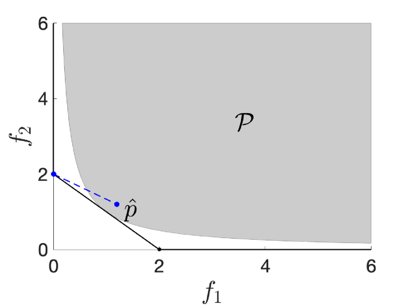
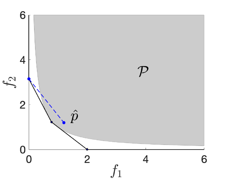
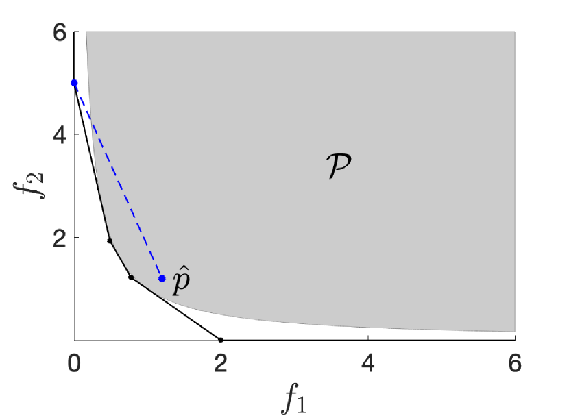
Figure 5: The outer approximations obtained after the first, second and third iterations of the KTW algorithm for Example 2 are shown, where $\hat{p}=(1.2,1.2)^{\mathsf{T}}$. In each figure, the selected vertex for the corresponding iteration is indicated. The minimal point to be found after the scalarization is the intersection of ${\rm bd\,}\mathcal{P}$ with the dashed line between the selected vertex and $\hat{p}$. Even though the approximation gets finer in each iteration, the distances found by the KTW algorithm are 0.7619, 0.7633 and 0.7803, respectively.

6.2 Computational results under limited runtime

In this set of experiments, we run Examples 1-5 under a runtime limit and report the proximity measures that the algorithms return in Table 6. For each example, around half of the shortest CPU time obtained in Section 6.1 is set as the time limit. For the variants UB, R, C and Adj, two different cardinality values are provided. The original value is greater (which is also equal to SC), whereas the smaller value is found by using Remark 4.1.

In Example 5, for $p=3$, we solve the same randomly generated instances that we solved in Section 6.1. Since the CPU times for these instances differ significantly, the most time-consuming 8 instances are selected, and the same runtime limit of 50 seconds is fixed for them. The corresponding results in Table 6 are the averages over the 8 instances.

Table 6: Computational results for Examples 1-5 when the algorithms run under runtime limit T.

	Example 1, $p=3$, T = 50				Example 1, $p=4$, T = 75				Example 2, T = 15
Algorithm	VS	Err	HG	Card	VS	Err	HG	Card	VS	Err	HG	Card
AUU	95	0.0168	0.13	29	154	0.0783	-	28	31	0.0296	32.37	15
DLSW	139	0.0136	0.09	36	234	0.0707	1.07	32	37	0.0346	34.54	15
KTW	129	0.0183	0.12	27	183	0.0771	-	30	-	-	-	-
UB	0	0.0057	0.04	124 (35)	0	0.0348	0.53	155 (80)	0	0.0283	0.90	44 (16)
R	0	0.0067	0.14	127.8 (44.4)	0	0.0338	0.55	169.2 (98.8)	0	0.0589	39.84	45 (16.2)
C	0	0.0054	0.09	120 (32)	0	0.0356	0.56	161 (95)	0	0.0129	12.46	42 (11)
Adj	0	0.0071	0.13	124 (32)	0	0.0359	0.66	166 (94)	0	0.0989	1.79	46 (27)
	Example 3, $a=5$, T = 15				Example 3, $a=7$, T = 15				Example 3, $a=10$, T = 15				Example 3, $a=20$, T = 15
	VS	Err	HG	Card	VS	Err	HG	Card	VS	Err	HG	Card	VS	Err	HG	Card
AUU	25	0.4119	18.37	10	28	0.4138	25.64	11	28	0.4033	38.89	11	25	0.6616	100.51	11
DLSW	42	0.4625	23.34	9	33	0.6168	19.73	12	42	0.4424	-	12	35	0.2958	59.14	13
KTW	35	0.2274	8.48	12	34	0.1839	5.83	16	37	0.1953	10.32	16	36	0.3164	25.38	16
UB	0	0.1744	2.76	34 (14)	0	0.2163	4.09	35 (9)	0	0.4800	-	36 (9)	0	0.3712	12.00	37 (6)
R	0	0.5984	5.21	35.8 (10)	0	0.2862	8.38	36.4 (9.2)	0	0.8142	18.76	37 (11.2)	0	0.4522	33.37	37.4 (11.8)
C	0	0.1057	2.54	35 (8)	0	0.1494	4.99	36 (10)	0	0.1672	5.38	37 (7)	0	0.1878	12.45	37 (10)
Adj	0	0.2059	3.08	31 (10)	0	0.4557	6.11	35 (14)	0	0.1850	5.91	34 (11)	0	0.5074	11.54	37 (9)
	Example 4, $a=5$, T = 250				Example 4, $a=7$, T = 250				Example 4, $a=10$, T = 250
	VS	Err	HG	Card	VS	Err	HG	Card	VS	Err	HG	Card
UB	0	0.1010	-	392 (233)	0	0.1261	7.23	366 (211)	0	0.1010	-	382 (214)
R	0	0.2072	-	508.5 (164.5)	0	0.1825	-	480.4 (318.4)	0	0.2759	-	498.6 (329)
C	0	0.1678	-	452 (304)	0	0.1013	-	424 (276)	0	0.3343	-	519 (361)
Adj	0	0.2072	-	537 (378)	0	0.1312	-	504 (349)	0	0.1518	-	513 (351)
	Example 5, $p=3$, T = 50 (avg)				Example 5, $p=4$, T = 100 (ins 1)				Example 5, $p=4$, T= 15 (ins 2)				Example 5, $p=4$, T = 50 (ins 3)
	VS	Err	HG	Card	VS	Err	HG	Card	VS	Err	HG	Card	VS	Err	HG	Card
AUU	69.125	1.3145	15966.61	22.13	318	2.7899	3453462.73	38	43	11.3862	415587.08	12	182	2.9557	722544.84	26
DLSW	72.375	2.1944	22167.71	20.25	338	3.1038	2776469.82	33	41	5.6440	224514.46	13	175	3.2645	803350.19	21
KTW	98	0.9805	11919.47	26.25	403	4.8830	3176108.34	30	57	10.2325	182864.48	13	194	1.5588	408030.61	30
UB	0	1.1396	32596.53	95.38 (25.63)	0	1.2209	-	269 (101)	0	3.0480	-	56 (20)	0	1.0328	37740.57	165 (66)
R	0	2.8557	3564.33	91.75 (22.13)	0	2.5621	-	286.4 (82.6)	0	8.6336	23599.91	55.4 (14.4)	0	3.1134	42125.39	163.8 (44)
C	0	0.9553	2825.69	89 (21)	0	1.4384	139495.18	266 (111)	0	1.7226	13700.71	55 (18)	0	0.8621	-	150 (50)
Adj	0	1.0659	3209.04	92.5 (29.63)	0	1.8833	268168.59	336 (182)	0	0.8027	19003.47	57 (20)	0	1.1001	46920.04	180 (88)

From Table 6, we observe that the solution sets returned by the variants (when Remark 4.1 is applied for UB, R, C and Adj) have similar cardinality values for two and three-dimensional examples. In Examples 2 and 3, C returned smaller approximation errors compared to the other variants, in general. In Example 1 with $p=3$, proposed variants return smaller error values compared to the variants from the literature, but in Example 5 with $p=3$, there is no clear conclusion.

For four-dimensional problems, AUU, DLSW, and KTW returned solution sets with smaller cardinality values than the others. In return, the approximation errors returned by AUU, DLSW, and KTW are larger than UB, C, and Adj for these problems. On the other hand, R behaves similarly to AUU, DLSW, and KTW. In most of the cases, HG values behave similarly to Err. However, in Example 5 for problems with $p=3$ and (ins 3) of $p=4$, the proposed variants return smaller HG, even though Err values are comparable among the algorithms.

An additional computational study is conducted on Example 3 to observe the behavior of the algorithms as the time limit changes. The variants are terminated after 50, 100 and 200 seconds. In this set of experiments, we also observe the effect of $\epsilon$ used within the variants UB, C, Adj and R even if the $\epsilon$ does not determine the stopping condition. Since we do not select the farthest away vertex to proceed with, $\epsilon$ has still an important role to decide if the algorithm would add a cut to the current outer approximation or not. To observe this effect, we run all the variants for the above-mentioned time limits both with $\epsilon=0.005$ and $\epsilon=0$. The results are provided in the appendix and the approximation errors obtained within different time limits for $a=5$ are shown in Figure 6b.

Figure 6: Approximation error results under runtime limits $T\in\{50,100,200\}$ for Example 3, $a=5$ when $\epsilon$ is taken as 0 (left) and 0.005 (right).

(a)

(b)

As expected, the performance of AUU, KTW and DLSW are not affected by the change in $\epsilon$. On the other hand, an increase in $\epsilon$ affects the performance of UB, C and Adj positively. R is affected less compared to UB, C and Adj, while UB is affected significantly. Note that the two variants that give the worst approximation error in each setting (UB and R for $\epsilon=0$ and R and DLSW for $\epsilon=0.005$) are not plotted to increase visibility.

6.3 Computational results under fixed cardinality

In this section, we compare the performances of the algorithms when they run until finding a solution set with a predetermined cardinality. For each example, we give a cardinality limit so that the algorithms terminate before reaching the approximation error that is set for the experiments in Section 6.1. In Example 5 where $p=3$, the same 8 instances are selected as in Section 6.2. For the variants UB, R, C, and Adj, we apply Remark 4.1. The results can be seen in Table 7.

Table 7: Computational results for Examples 1-5 when the algorithms run until finding a solution set with predetermined cardinality (Card).

	Example 1, $p=3$, Card $=100$				Example 1, $p=4$, Card $=50$				Example 2, Card $=20$
Algorithm	VS	T	Err	HG	VS	T	Err	HG	VS	T	Err	HG
AUU	451	252.12	0.0062	0.03	401	197.53	0.0578	0.51	64	29.15	0.0197	14.98
DLSW	455	175.98	0.0065	0.03	430	144.85	0.0579	0.52	90	34.97	0.0188	16.06
KTW	695	266.51	0.0067	0.03	816	327.38	0.0614	-	-	-	-	-
UB	0	93.74	0.0196	0.03	0	62.20	0.1448	-	0	15.83	0.0283	11.77
R	0	51.98	0.0325	0.07	0	48.24	0.4142	1.13	0	16.81	0.2236	32.63
C	0	90.66	0.0195	0.07	0	54.12	0.0894	0.49	0	21.45	0.0129	81.53
Adj	0	84.96	0.0116	0.04	0	48.75	0.1281	1.02	0	11.72	0.0989	-
	Example 3, $a=5$, Card $=30$				Example 3, $a=7$, Card $=30$				Example 3, $a=10$, Card $=30$				Example 3, $a=20$, Card $=30$
	VS	T	Err	HG	VS	T	Err	HG	VS	T	Err	HG	VS	T	Err	HG
AUU	98	50.51	0.0789	3.88	100	50.48	0.0789	4.32	104	52.06	0.0874	8.37	123	59.48	0.0877	15.77
DLSW	581	174.80	0.0979	4.22	106	41.22	0.1112	4.86	505	150.75	0.1122	7.70	104	41.40	0.1264	15.61
KTW	106	106.15	0.0543	1.96	102	78.82	0.0682	2.83	97	71.16	0.0639	4.07	116	76.91	0.0945	10.21
UB	0	25.14	0.0629	2.94	0	25.78	0.2163	6.36	0	26.66	0.1056	6.43	0	26.85	0.1256	7.29
R	0	25.27	0.1752	6.88	0	24.84	0.1677	8.97	0	25.59	0.2086	13.38	0	26.26	0.3129	15.93
C	0	24.32	0.1006	3.63	0	25.87	0.1184	5.71	0	26.10	0.1105	6.78	0	25.18	0.1827	7.98
Adj	0	23.34	0.1020	4.39	0	21.31	0.4557	7.82	0	24.69	0.1535	11.55	0	24.97	0.5069	7.84
	Example 4, $a=5$, Card $=100$				Example 4, $a=7$, Card $=100$				Example 4, $a=10$, Card $=100$
	VS	T	Err	HG	VS	T	Err	HG	VS	T	Err	HG
UB	0	137.56	0.1221	-	0	131.28	0.1261	-	0	145.59	0.2072	-
R	0	112.89	0.4142	16.22	0	113.22	0.3092	-	0	115.72	0.4101	-
C	0	142.94	0.1039	9.28	0	148.59	0.1530	17.54	0	129.40	0.3343	-
Adj	0	100.93	0.175	7.48	0	99.75	0.2072	-	0	113.33	0.2226	-
	Example 5, $p=3$, Card $=50$ (avg)				Example 5, $p=4$, Card $=125$ (ins 1)				Example 5, $p=4$, Card $=40$ (ins 2)				Example 5, $p=4$, Card $=75$ (ins 3)
	VS	T	Err	HG	VS	T	Err	HG	VS	T	Err	HG	VS	T	Err	HG
AUU	204	72.53	0.2502	5573.2	2533	768.70	0.229	606958.2	266	87.09	0.4871	30354.2	1207	386.52	0.4436	121479.4
DLSW	233	81.98	0.4715	3567.4	3042	904.62	0.348	163459.1	298	95.81	0.3892	12517.2	2027	363.61	0.5809	79236.2
KTW	347.75	94.26	0.2564	4484.0	6457	1641.78	0.256	605558.1	609	156.71	0.2523	24715.2	1167	534.57	0.3119	138802.3
UB	0	41.84	0.3672	1025.2	0	110.63	1.221	163636.9	0	25.16	0.4871	4128.8	0	58.71	1.0328	27890.2
R	0	43.31	1.0093	1325.7	0	127.41	1.206	40282.1	0	26.85	0.3716	1112.3	0	65.57	0.9916	10856.6
C	0	46.17	0.4707	1051.4	0	106.68	0.450	118499.2	0	26.84	0.2489	876.6	0	63.51	0.8274	89151.3
Adj	0	36.08	0.6722	1860.9	0	79.83	1.883	331493.0	0	24.36	0.1966	1636.87	0	47.58	1.1001	54859.5

In line with the observations from Section 6.1, we observe from Table 7 that UB, R, C, and Adj require less CPU time compared to AUU, DLSW, and KTW. Among the algorithms from Section 4.4, DLSW requires less CPU time compared to AUU and KTW, especially if the dimension of the objective space is high. When we compare the proposed variants, we see that Adj is slightly faster than the others in most examples.

The approximation errors obtained by AUU, DLSW, and KTW are smaller than or very close to those obtained by UB, R, C, and Adj, in general. This shows the trade-off between the runtime and approximation error. When we compare the algorithms from Section 4.4, AUU and KTW yield better results in terms of the approximation error compared to DLSW, in general. On the other hand, the variants UB, R, C, and Adj are comparable among themselves. When we consider the HG values, we observe a similar behavior as Err, especially for problems with $p\in\{2,3\}$. However, in Example 5 the proposed variants return smaller HG values even though the Err values are slightly worse than or comparable with the algorithms from the literature.

7 Conclusion

We consider bounded convex vector optimization problems and present a general framework for existing outer approximation algorithms from the literature. We observe that many algorithms iterate by solving Pascoletti-Serafini scalarizations or equivalent models and they mainly differ in selecting the parameters of the scalarization in each iteration. We propose additional methods to select the reference point (a vertex of the current outer approximation) and direction parameter of this scalarization.

First, for a given vertex, we propose two methods to select the direction parameter. These methods are based on the position of the selected vertex as well as (1) the ideal point and (2) the adjacent vertices of the selected vertex, respectively. We compare the proposed direction selection rules together with the ones commonly used in the literature through preliminary computational tests and observe that using the positions of the adjacent vertices yields promising results. Hence, if the vertex enumeration problems are solved based on the double description method (e.g. by bensolve) so that the adjacency information is already obtained, then using Adj to select the direction parameter for each vertex is preferable.

We also propose some vertex selection rules which, different from the existing ones in the literature, do not require solving additional optimization problems. Instead, the proposed selection methods use the positions of all vertices (1) to form clusters and select accordingly, (2) to pick the most isolated vertex, or (3) to find the farthest away vertex from its corresponding local upper bound, respectively.

We implement the proposed vertex selection procedures together with the direction selection rule Adj and three relevant approaches from the literature. We provide an extensive computational study and observe that especially when the ordering cone is the positive orthant or a larger cone, the proposed variants perform better in terms of CPU time if the stopping condition is the approximation error or the cardinality of the solution set. On the other hand, the CPU times are comparable when the ordering cone is a strict subset of the positive orthant.

When the algorithms are run under a time limit, the proximity measures returned by the proposed variants are either better than or comparable to the ones returned by the algorithms from the literature. We also observe that the selection of $\epsilon$ affects the performance of the proposed variants even when $\epsilon$ is not used as the stopping criterion.

We conclude that if a reasonably good direction selection method (e.g. Adj) is used in the algorithm, then the vertex selection rule may have less impact on the performance of the algorithm. Hence, solving additional single objective optimization problems to select a vertex may not be necessary to improve the performance of the algorithm.

When we compare the overall performances of the proposed vertex selection methods, there is no clear conclusion. Indeed, random selection works very well in many cases, especially if the stopping condition is the approximation error. However, there are also some cases for which R works considerably worse than the proposed variants, see for instance the results for Examples 3 and 5 when the algorithms run until a predetermined runtime or cardinality limit (Tables 6, 7). In that sense, we conclude that R may not be as robust as the proposed variants, as expected. As a final remark, note that if the ordering cone is the positive orthant, then using UB has an advantage as it also returns an upper bound for the current approximation error when it is terminated after a predetermined runtime or cardinality limit.

Appendix A Testing different direction selection rules for UB

Even though we fix Adj as the direction selection rule for further computational study in Section 5.2, we note that when UB is used as the vertex selection rule, it is possible to use the local upper bounds in order to determine the direction parameter as well. In particular, for a vertex $v$ with the corresponding local upper bound $u$, we consider selecting the direction parameter as the vector from $v$ to $u$. In order to test this direction selection rule we conduct a computational study on Example 3 in which we compare three direction selection rules: $d=\frac{e}{\left\|e\right\|}$ (UB-FD), $d=\frac{(u-v)}{\left\|u-v\right\|}$ (UB-UB), and adjacent vertices approach (UB-Adj). We observe in Table 8 that UB-Adj solves less number of scalarizations while UB-UB clearly has a negative effect on T and SC. Based on this preliminary analysis, we confirm the usage of Adj as the direction selection rule throughout the computational studies in Section 6.

Table 8: The effect of different direction selection methods for UB for Ex 3 with $\epsilon=0.05$

	$a=5$			$a=7$			$a=10$			$a=20$
	UB-FD	UB-UB	UB-Adj	UB-FD	UB-UB	UB-Adj	UB-FD	UB-UB	UB-Adj	UB-FD	UB-UB	UB-Adj
SC	128	547	110	127	570	112	139	737	90	194	1990	127
T	38.83	173.58	32.51	36.81	178.73	33.36	41.20	240.06	26.93	62.16	996.51	37.44

Appendix B Vertex selection procedures of the existing algorithms from Section 4.4

$$\textrm{maximize }\lambda\>\>\textrm{subject to }f(x)\leq\hat{p}+\lambda(v-\hat{p}),\>x\in\mathcal{X},\>\lambda\in\mathbb{R}.$$ (7)

Procedure 8 SelectVertex($V^{k}$,$V_{\textnormal{used}}\,$,$V^{k}_{\textnormal{info}}\,$) of Algorithm KTW

1:  $V_{\textnormal{info}}^{\textnormal{temp}}=\emptyset$

2:  for all $v\in V^{k}\setminus V_{\textnormal{used}}\,$ do

3:     if $(v,y^{v},z^{v})\notin V^{k}_{\textnormal{info}}\,$ then

4:        Let ($x^{v},\lambda^{v}$) be a solution to (7), $y^{v}:=\hat{p}+\lambda^{v}(v-\hat{p})$ and $z^{v}:=\left\|y^{v}-v\right\|$;

5:     end if

6:     $V_{\textnormal{info}}^{\textnormal{temp}}\leftarrow V_{\textnormal{info}}^{\textnormal{temp}}\cup\{(v,y^{v},z^{v})\}$;

7:  end for

8:  $V^{k}_{\textnormal{info}}\,\leftarrow V_{\textnormal{info}}^{\textnormal{temp}}$;

9:  Let $v^{*}\in\operatorname*{arg\,max}_{(v,y^{v},z^{v})\in\mathcal{V}^{k}}z^{v}$;

10:  return  $v^{*}$, $V^{k}_{\textnormal{info}}\,$

$$\textrm{minimize }\left\|y-v\right\|^{2}\>\>\textrm{subject to }y\in\mathcal{I}^{k}.$$ (8)

Procedure 9 SelectVertex($x^{k}$,$V^{k}$,$V_{\textnormal{used}}\,$,$V^{k}_{\textnormal{info}}\,$) of Algorithm DLSW

1:  $V_{\textnormal{info}}^{\textnormal{temp}}=\emptyset$

2:  for all $v\in V^{k}\setminus V_{\textnormal{used}}\,$ do

3:     if  $(v,y^{v},z^{v})\in V^{k}_{\textnormal{info}}\,$ then

4:        if $(y^{v}-v)^{\mathsf{T}}(f(x^{k})-y^{v})<0$ then

5:           Solve (8) and for the vertex $v$ find $y^{v}\in\mathcal{I}^{k}$;

6:        end if

7:     else

8:        Solve (8) and for the vertex $v$ find $y^{v}\in\mathcal{I}^{k}$;

9:     end if

10:     $V_{\textnormal{info}}^{\textnormal{temp}}\leftarrow V_{\textnormal{info}}^{\textnormal{temp}}\cup\{(v,y^{v},z^{v})\}$;

11:  end for

12:  $V^{k}_{\textnormal{info}}\,\leftarrow V_{\textnormal{info}}^{\textnormal{temp}}$;

13:  Let $v^{*}\in\operatorname*{arg\,max}_{(v,y^{v},z^{v})\in\mathcal{V}^{k}}z^{v}$;

14:  return  $v^{*}$, $V^{k}_{\textnormal{info}}\,$

$$\textrm{minimize }\left\|z\right\|\>\>\textrm{subject to }f(x)\leq_{C}v+z,\>x\in\mathcal{X},z\in\mathbb{R}^{p}.$$ (9)

Procedure 10 SelectVertex($V^{k}$,$V_{\textnormal{used}}\,$,$V^{k}_{\textnormal{info}}\,$) of Algorithm AUU

1:  $V_{\textnormal{info}}^{\textnormal{temp}}=\emptyset$;

2:  for all $v\in V^{k}\setminus V_{\textnormal{used}}\,$ do

3:     if $(v,y^{v},z^{v})\notin V^{k}_{\textnormal{info}}\,$ then

4:        Let $z^{v}$ be a solution to (9);

5:     end if

6:     $V_{\textnormal{info}}^{\textnormal{temp}}\leftarrow V_{\textnormal{info}}^{\textnormal{temp}}\cup\{(v,y^{v},z^{v})\}$;

7:  end for

8:  $V^{k}_{\textnormal{info}}\,\leftarrow V_{\textnormal{info}}^{\textnormal{temp}}$;

9:  Let $v^{*}\in\operatorname*{arg\,max}_{(v,y^{v},z^{v})\in\mathcal{V}^{k}}z^{v}$;

10:  return  $v^{*}$, $V^{k}_{\textnormal{info}}\,$

Appendix C An example with different ordering cones

Consider Example 1 for $p\in\{2,3\}$ with the following ordering cones:
$C_{1}={\rm co\,}{\rm conv\,}\{(1,2)^{\mathsf{T}},(2,1)^{\mathsf{T}}\}\subsetneq\mathbb{R}^{2}_{+},\\ C_{2}=C_{1}^{+}={\rm co\,}{\rm conv\,}\{(2,-1)^{\mathsf{T}},(-1,2)^{\mathsf{T}}\}\supsetneq\mathbb{R}^{2}_{+},\\ C_{3}={\rm co\,}{\rm conv\,}\{(-1,-1,3)^{\mathsf{T}},(2,2,-1)^{\mathsf{T}},(1,0,0)^{\mathsf{T}},(0,-1,2)^{\mathsf{T}},(-1,0,2)^{\mathsf{T}},(0,1,0)^{\mathsf{T}}\}\supsetneq\mathbb{R}^{3}_{+},\\ C_{4}=C_{3}^{+}={\rm co\,}{\rm conv\,}\{(4,2,2)^{\mathsf{T}},(2,4,2)^{\mathsf{T}},(4,0,2)^{\mathsf{T}},(1,0,2)^{\mathsf{T}},(0,1,2)^{\mathsf{T}},(0,4,2)^{\mathsf{T}}\}\subsetneq\mathbb{R}^{3}_{+}$.
Figure 7 provides illustrations of the outer approximations of the upper image for $p=3$ with ordering cones $C_{3}$ and $C_{4}$.

Figure 7: The outer approximations of the upper image of Example 1 for $p=3$ with cones $C_{3}$ (left) and $C_{4}$ (right) obtained by Algorithm Adj, where the stopping condition is taken as $\epsilon=0.01$.

Since algorithms KTW and UB are designed to solve multiobjective optimization problems, they are not included in this set of experiments. Table 9 shows the performances of AUU, DLSW, R, C, and Adj under different stopping criteria. Different from the main set of experiments, the bounding set $\mathcal{Q}$ considered for HG calculations is computed exactly as in [1, Section 6.1]. Also, these experiments are conducted using a different computer with specifications: Intel(R) Core(TM) i7-8565U CPU @ 1.80GHz.

Table 9: Computational results for Example 1 for $p=2$ with ordering cones $C_{1}$ and $C_{2}$, and for $p=3$ with ordering cones $C_{3}$ and $C_{4}$. The first set (fixed $\epsilon$) shows the results when the algorithms run until returning a finite weak $\epsilon$-solution for provided $\epsilon$ values; the second set (fixed T) shows the results when the algorithms run under runtime limit T, and the third set shows the results when the algorithms run until finding a solution set with predetermined cardinality (Card).

		$p=2,\ C_{1}$				$p=2,\ C_{2}$				$p=3,\ C_{3}$				$p=3,\ C_{4}$
		$\epsilon=0.0005$				$\epsilon=0.0005$				$\epsilon=0.01$				$\epsilon=0.01$
	Algorithm	VS	SC	T	HG	VS	SC	T	HG	VS	SC	T	HG	VS	SC	T	HG
fixed $\epsilon$	AUU	87	45	25.93	0.0109	38	17	10.72	0.00023	145	43	46.24	0.00007	378	81	105.58	0.2434
	DLSW	104	45	23	0.0054	37	17	8.48	0.00001	310	75	65.96	0.00002	1109	148	196.43	0.0949
	R	0	129.2	24.46	0.0003	0	33.4	6.20	0.00004	0	106.6	23.32	0.00005	0	509	110.49	0.0225
	C	0	131	24.07	0.0003	0	33	5.69	0.00006	0	114	28.25	0.00004	0	483	112.72	0.0271
	Adj	0	129	24.39	0.0003	0	33	6.04	0.00006	0	115	27.61	0.00003	0	601	137.42	0.0202
		T=15				T=5				T=15				T=15
		VS	Card	Err	HG	VS	Card	Err	HG	VS	Card	Err	HG	VS	Card	Err	HG
fixed T	AUU	53	28	0.0008	0.0116	19	11	0.0008	0.00008	45	13	0.0289	0.0012	166	36	0.0256	-
	DLSW	81	38	0.0008	0.0057	25	14	0.0008	0.00004	79	18	0.0165	0.0007	293	54	0.0205	0.0006
	R	0	56.2	0.0015	0.0013	0	16	0.0002	0.00001	0	31.2	0.0150	0.0003	0	126.2	0.0265	0.0001
	C	0	61	0.0015	0.0005	0	15	0.0002	0.00001	0	23	0.0162	0.0003	0	120	0.0226	0.0001
	Adj	0	62	0.0004	0.0003	0	16	0.0002	0.00001	0	35	0.0147	0.0003	0	129	0.0232	0.0003
		Card=30				Card=10				Card=20				Card=40
		VS	T	Err	HG	VS	T	Err	HG	VS	T	Err	HG	VS	T	Err	HG
fixed Card	AUU	55	14.34	0.0004	0.0116	15	4.74	0.0008	0.00008	55	17.05	0.0437	0.0016	161	51.04	0.0262	-
	DLSW	67	14.43	0.0008	0.0060	19	5.05	0.0008	0.00005	90	26.81	0.0147	0.0008	203	45.06	0.0207	0.0006
	R	0	11.62	0.0015	0.0034	0	4.20	0.0002	0.00001	0	10.31	0.0598	0.0006	0	33.66	0.0609	0.0001
	C	0	13.63	0.0015	0.0005	0	5.03	0.0002	0.00001	0	11.47	0.0530	0.0004	0	46.07	0.0255	0.0001
	Adj	0	13.12	0.0004	0.0004	0	4.01	0.0002	0.00001	0	11.78	0.0240	0.0005	0	33.08	0.0493	-

From Table 9, we observe that if the algorithms run until they return a finite weak $\epsilon$-solution (fixed $\epsilon$), then similar to the observations from Section 6, the proposed variants are faster than the algorithms from the literature for the ordering cones larger than the positive orthant ($C_{2},C_{3}$). However, there is no clear conclusion for the ordering cones smaller than the positive orthant.

Under fixed runtime (fixed T), we observe that AUU and DLSW return solution sets with smaller cardinality. The algorithms are comparable in terms of the Err that they return. Moreover, AUU consistently yields the worst HG value and R, C and Adj return slightly better HG values than DLSW.

Finally, when the algorithms run until they find a predetermined number of solutions (fixed Card), the proposed variants return smaller HG values compared to AUU and DLSW. However, T and Err values are comparable for all algorithms.

Appendix D Results for different runtime limits for Example 3

Table 10: Computational results for Example 3 when the algorithms run under different runtime limits T$\in\{50,100,200\}$.

		Example 3, $a=5$						Example 3, $a=7$
		Err		HG		Card		Err		HG		Card
		$\epsilon=0$	$\epsilon=0.005$	$\epsilon=0$	$\epsilon=0.005$	$\epsilon=0$	$\epsilon=0.005$	$\epsilon=0$	$\epsilon=0.005$	$\epsilon=0$	$\epsilon=0.005$	$\epsilon=0$	$\epsilon=0.005$
T=50	AUU	0.061	0.061	2.5348	2.5348	38	38	0.0635	0.0633	3.6097	3.4895	37	38
	DLSW	0.1428	0.1159	7.4127	7.2898	19	20	0.0577	0.0577	3.3893	3.3893	45	45
	KTW	0.0633	0.0633	1.4557	1.586	43	42	0.0689	0.0689	2.0931	2.0931	43	43
	UB	0.415	0.0489	5.4621	0.6262	154	164 (44)	0.2163	0.078	2.5031	0.9474	150	164 (44)
	R	0.201	0.1922	2.7797	1.9551	156	161.8 (27.8)	0.5199	0.1298	6.977	4.3267	158	161.6 (26.2)
	C	0.0925	0.0472	1.1053	0.7466	133	162 (26)	0.0659	0.0659	1.0019	1.0321	159	157 (34)
	Adj	0.0775	0.0709	0.6087	0.6229	156	161 (26)	0.0658	0.0658	0.7674	0.7543	159	163 (28)
T=100	AUU	0.0293	0.0319	1.5539	1.5924	59	58	0.0394	0.0393	2.4166	2.4045	48	49
	DLSW	0.098	0.098	3.3152	3.3694	28	27	0.0333	0.0333	1.372	1.372	82	82
	KTW	0.0355	0.0355	0.8512	0.8469	71	72	0.0448	0.0448	2.5774	2.5774	68	68
	UB	0.415	0.0489	5.4621	0.3433	248	249 (72)	0.2163	0.0286	2.3386	-	240	261 (81)
	R	0.1433	0.087	1.0544	1.4441	283	323.2 (114.4)	0.2185	0.0732	2.042	1.3026	285	322.6 (106.6)
	C	0.0448	0.0447	0.4774	0.3685	281	326 (111)	0.0455	0.0659	0.51	0.6218	281	314 (103)
	Adj	0.0422	0.0329	0.2926	0.29	280	319 (112)	0.0382	0.0345	0.4494	0.3984	287	323 (115)
T=200	AUU	0.016	0.0151	0.6718	0.6417	109	114	0.0352	-	1.265	-	130	-
	DLSW	0.0546	0.0546	2.4949	2.3092	40	41	0.0201	0.0201	0.7286	0.7329	154	154
	KTW	0.0213	0.0213	0.5353	0.4808	122	128	0.0225	0.0225	0.6514	0.667	129	129
	Ub	0.415	0.0108	5.462	0.1769	421	545 (275)	-	0.0148	-	-	-	427 (277)
	R	0.1089	0.0405	1.6491	0.2699	464.6	650.2 (285.2)	0.1281	0.0197	5.9576	0.6547	466.6	466.6 (297.8)
	C	0.0448	0.0228	0.3711	0.2064	474	650 (279)	0.0276	0.0659	0.5335	0.436	472	472 (288)
	Adj	0.0405	0.0178	0.1778	0.177	463	641 (302)	0.0374	0.0185	0.8885	0.394	469	469 (304)
		Example 3, $a=10$						Example 3, $a=20$
		Err		HG		Card		Err		HG		Card
		$\epsilon=0$	$\epsilon=0.005$	$\epsilon=0$	$\epsilon=0.005$	$\epsilon=0$	$\epsilon=0.005$	$\epsilon=0$	$\epsilon=0.005$	$\epsilon=0$	$\epsilon=0.005$	$\epsilon=0$	$\epsilon=0.005$
T=50	AUU	0.0603	0.0603	5.2053	5.2053	38	38	0.0789	0.0789	12.7094	11.3389	33	33
	DLSW	0.1802	0.1802	8.6532	8.6532	23	23	0.0762	0.0741	8.8851	8.6309	45	46
	KTW	0.064	0.0835	2.0931	3.243	48	42	0.0945	0.0945	5.8671	5.8671	45	45
	UB	0.5282	0.0996	-	1.1499	155	160 (38)	0.3833	0.123	37.5565	3.9389	136	155 (34)
	R	0.184	0.1225	5.8429	4.0538	157.8	160 (28.4)	0.2774	0.2773	22.452	25.2676	157.4	161 (22.8)
	C	0.1105	0.139	1.4924	1.5941	158	154 (22)	0.1079	0.1303	3.6095	7.1808	155	164 (38)
	Adj	0.1004	0.1004	1.3138	1.5617	159	162 (30)	0.2199	0.1601	4.2782	5.4184	157	163 (23)
T=100	AUU	0.03	0.0305	2.6334	2.6359	69	68	0.0335	0.0339	5.9792	5.9851	67	66
	DLSW	0.1122	0.1122	7.8622	7.704	29	30	0.037	0.037	4.6299	4.7261	86	85
	KTW	0.0635	0.0561	2.1896	1.9612	54	58	0.0774	0.0774	3.2962	3.3143	77	76
	UB	0.5282	0.0584	20.5524	0.5731	254	257 (77)	0.3833	0.0584	37.5564	1.5682	268	292 (85)
	R	0.3065	0.0929	10.6075	1.0173	282.8	316.8 (95.4)	0.0985	0.1333	4.409	5.6698	312.8	312.8 (91)
	C	0.0444	0.0422	0.9645	0.8517	267	312 (102)	0.0472	0.0931	1.8988	1.9479	277	319 (126)
	Adj	0.0477	0.0477	0.6971	0.5908	283	323 (110)	0.1594	0.0903	2.0781	1.3881	285	315 (95)
T=200	AUU	0.0221	0.0222	1.5587	1.5863	92	90	-	-	-	-	-	-
	DLSW	0.0588	0.0603	4.8736	5.3437	58	57	0.0204	0.0204	2.0845	2.0861	158	157
	KTW	0.0425	0.0425	1.2532	1.2717	116	115	0.0774	0.0774	2.8347	2.8347	92	92
	Ub	0.5282	0.0154	20.5524	0.3031	423	541 (296)	0.3832	0.0239	32.564	0.7241	423	522 (286)
	R	0.0899	0.0839	1.2446	0.4661	463	628.8 (299.6)	0.0778	0.0606	4.2709	1.6708	464	619 (320.4)
	C	0.0366	0.0422	0.3878	0.3943	467	640 (296)	0.0469	0.0168	2.3304	2.0154	466	632 (299)
	Adj	0.0438	0.0319	0.3796	0.2962	468	623 (314)	0.0903	0.0476	1.6607	1.0872	465	611 (330)

References

- [1] Ç. Ararat, S. Tekgül, and F. Ulus. A new geometric duality and geometric dual algorithm for convex vector optimization problems. To appear in: SIAM Journal on Optimization, arxiv preprint no: 2108.07053, 2022.
- [2] Ç. Ararat, F. Ulus, and M. Umer. A norm minimization-based convex vector optimization algorithm. Journal of Optimization Theory and Applications, 194:681–712, 2022.
- [3] T. Bektaş. Disjunctive programming for multiobjective discrete optimisation. INFORMS Journal on Computing, 30:625–633, 2018.
- [4] H. P. Benson. An outer approximation algorithm for generating all efficient extreme points in the outcome set of a multiple objective linear programming problem. Journal of Global Optimization, 13:1–24, 1998.
- [5] K. Dächert and K. Klamroth. A linear bound on the number of scalarizations needed to solve discrete tricriteria optimization problems. Journal of Global Optimization, 61:643–676, 2015.
- [6] D. Dörfler, A. Löhne, C. Schneider, and B. Weißing. A Benson-type algorithm for bounded convex vector optimization problems with vertex selection. Optimization Methods and Software, 37(3):1006–1026, 2022.
- [7] M. Ehrgott, L. Shao, and A. Schöbel. An approximation algorithm for convex multi-objective programming problems. Journal of Global Optimization, 50(3):397–416, 2011.
- [8] S. Gass and T. Saaty. The computational algorithm for the parametric objective function. Naval research logistics quarterly, 2(1-2):39–45, 1955.
- [9] M. Grant and S. Boyd. Graph implementations for nonsmooth convex programs. In V. Blondel, S. Boyd, and H. Kimura, editors, Recent Advances in Learning and Control, Lecture Notes in Control and Information Sciences, pages 95–110. Springer-Verlag Limited, 2008.
- [10] M. Grant and S. Boyd. CVX: Matlab software for disciplined convex programming. http://cvxr.com/cvx, March 2014.
- [11] A. Hamel, B. Rudloff, and M. Yankova. Set-valued average value at risk and its computation. Mathematics and Financial Economics, 7(2):229–246, 2013.
- [12] T. Holzmann and J. C. Smith. Solving discrete multi-objective optimization problems using modified augmented weighted Thebychev scalarizations. European Journal of Operational Research, 30:436–449, 2018.
- [13] J. Jahn. Vector Optimization - Theory, Applications, and Extensions. Springer, 2004.
- [14] K. Klamroth, J. Tind, and M. M. Wiecek. Unbiased approximation in multicriteria optimization. Mathematical Methods of Operations Research, 56:413–437, 2003.
- [15] A. Löhne. Vector Optimization with Infimum and Supremum. Springer, 2011.
- [16] A. Löhne, B. Rudloff, and F. Ulus. Primal and dual approximation algorithms for convex vector optimization problems. Journal of Global Optimization, 60(4):713–736, 2014.
- [17] A. Löhne and B. Weißing. BENSOLVE: A free VLP solver, version 2.0.1. http://bensolve.org/, 2015.
- [18] A. Löhne and B. Weißing. The vector linear program solver bensolve–notes on theoretical background. European Journal of Operational Research, 260(3):807–813, 2017.
- [19] D. Luc. Theory of Vector Optimization, volume 319 of Lecture Notes in Economics and Mathematical Systems. Springer Verlag, 1989.
- [20] A. Pascoletti and P. Serafini. Scalarizing vector optimization problems. Journal of Optimization Theory and Applications, 42(4):499–524, 1984.
- [21] R. T. Rockafellar. Convex Analysis. Princeton University Press, 1970.
- [22] B. Rudloff and F. Ulus. Certainty equivalent and utility indifference pricing for incomplete preferences via convex vector optimization. Mathematics and Financial Economics, 15(2):397–430, 2021.
- [23] J. F. Sturm. Using SeDuMi 1.02, a MATLAB toolbox for optimization over symmetric cones. Optimization Methods and Software, 11–12:625–653, 1999.
- [24] E. Zitzler and L. Thiele. Multiobjective evolutionary algorithms: a comparative case study and the strength Pareto approach. IEEE transactions on Evolutionary Computation, 3(4):257–271, 1999.