Backward diffusion-wave problem: stability, regularization and approximation

Abstract

We aim at the development and analysis of the numerical schemes for approximately solving the backward diffusion-wave problem, which involves a fractional derivative in time with order $\alpha\in(1,2)$. From terminal observations at two time levels, i.e., $u(T_{1})$ and $u(T_{2})$, we simultaneously recover two initial data $u(0)$ and $u_{t}(0)$ and hence the solution $u(t)$ for all $t>0$. First of all, existence, uniqueness and Lipschitz stability of the backward diffusion-wave problem were established under some conditions about $T_{1}$ and $T_{2}$. Moreover, for noisy data, we propose a quasi-boundary value scheme to regularize the ”mildly” ill-posed problem, and show the convergence of the regularized solution. Next, to numerically solve the regularized problem, a fully discrete scheme is proposed by applying finite element method in space and convolution quadrature in time. We establish error bounds of the discrete solution in both cases of smooth and nonsmooth data. The error estimate is very useful in practice since it indicates the way to choose discretization parameters and regularization parameter, according to the noise level. The theoretical results are supported by numerical experiments.

1 Introduction

Let $\Omega\subset\mathbb{R}^{d}$ ($d=1,2,3$) be a convex polyhedral domain with boundary $\partial\Omega$. We consider the following initial-boundary value problem of diffusion-wave equation with $\alpha\in(1,2)$

$$\begin{aligned} {\partial_{t}^{\alpha}}u-\Delta u&=f,\ &&\text{in}\ \Omega\times(0,T],\\ u&=0,\ &&\text{on}\ \partial\Omega,\\ u(0)=a,~{}\partial_{t}u(0)&=b,\ &&\text{in}\ \Omega,\\ \end{aligned}$$ (1)

where $T>0$ is a fixed final time, $f\in L^{\infty}(0,T;L^{2}(\Omega))$ and $a,b\in L^{2}(\Omega)$ are given source term and initial data, respectively, and $\Delta$ denotes the Laplace operator in space. Here ${\partial_{t}^{\alpha}}u(t)$ denotes the Caputo fractional derivative in time $t$ of order $\alpha\in(1,2)$ [19, p. 70]

$${\partial_{t}^{\alpha}}u(t)=\frac{1}{\Gamma(2-\alpha)}\int_{0}^{t}(t-s)^{1-\alpha}\tfrac{\partial^{2}}{\partial s^{2}}u(s){\rm d}s.$$

In recent years, there has been a growing interest in fractional / nonlocal models due to their diverse applications in physics, engineering, biology and finance. Specifically, the time-fractional diffusion equations ($\alpha\in(0,1)$) are often used to model subdiffusion phenomena in media with highly heterogeneous aquifers [1, 10] and fractal geometry [37], while the time-fractional diffusion-wave equations (1) ($\alpha\in(1,2)$) are frequently used to describe the propagation of mechanical waves in viscoelastic media [31, 32]. We refer interested readers to [34, 35] for a long list of applications of fractional models arising from biology and physics.

Inverse problems for fractional evolution models have attracted much interest, and there has already been a vast literature; see e.g., review papers [18, 23, 24, 28] and references therein. The aim of this paper is to investigate the backward problem for the diffusion-wave model (1): (IP) we simultaneously determine the initial data $u(x,0)$ and $u_{t}(x,0)$ with $x\in\Omega$ (and hence the function $u(x,t)$ for all $(x,t)\in\Omega\times(0,T)$) from two terminal observations

$$u(x,T_{1})=g_{1}(x),\quad u(x,T_{2})=g_{2}(x)\quad\text{for all}~{}~{}x\in\Omega,$$

where $T_{1},T_{2}\in(0,T]$ and $T_{1}<T_{2}$.

The study on the backward problem for the diffusion-wave model remains fairly scarce. In [47] Wei and Zhang studied the backward problem to recover a single initial condition $u(0)$ or $u_{t}(0)$ (with the other one known) from the single terminal data $u(T)$. Floridia and Yamamoto analyzed the simutaneous recovery of two initial data from two terminal observations $u(T)$ and $u_{t}(T)$, and established a Lipschitz stability in [8]. In the setting of current paper, we consider two observations $u(T_{1})$ and $u(T_{2})$, which are practical in many empirical experiments. As far as we know, there is no rigorous analysis of the discretized (numerical) scheme for solving the backward problem (IP)where some regularization error and discretization error(s) will be introduced into the system. Then there arises a natural question: is it possible to derive an a priori error estimate, showing the way to to balance discretization error, regularization parameter and the noise? However, such an analysis remains unavailable, and it is precisely this gap that the project aims to fill in.

The backward subdiffusion problem ($\alpha\in(0,1)$) has been intensively studied in recent years, where the single initial condition $u(0)$ is determined from the single observation $u(T)$. See e.g. [39, 43] for the uniqueness and some stability estimate, [27, 45, 49, 46] for some regularization methods, and [51] for error analysis of fully discrete schemes. Compared with the subdiffusion problem, the initial layer near $t=0$ is more singular for the diffusion wave model, in sense that

$$\|u(t)\|_{\dot{H}^{2}(\Omega)}+\|\partial_{t}^{\alpha}u(t)\|_{L^{2}(\Omega)}\leq ct^{-\alpha}\Big{(}\|u(0)\|_{L^{2}(\Omega)}+t\|u_{t}(0)\|_{L^{2}(\Omega)}\Big{)},$$

that clearly indicates a stronger singularity for $\alpha\rightarrow 2$. This brings more challenges in both numerical approximation and analysis. Besides, the mathematical and numerical analysis of the backward subdiffusion problem heavily rely on the completely monotonicity of the Mittag–Leffler function $E_{\alpha,1}(-z)$ or its discrete analogue, which is not valid for $\alpha\in(1,2)$. Therefore, the well-posedness of the backward problem requires additional conditions on the terminal time levels $T_{1}$ and $T_{2}$. This contrasts sharply with the subdiffusin counterpart ($\alpha\in(0,1)$), where the existence, uniqueness and two-side Lipschitz stability hold valid for any observation $u(T)$ with $T>0$.

In the first part of this paper, we show the well-posedness of the backward diffusion-wave problem. In particular, using the asymptotic behavior of Mittag-Leffler functions, we show that, under some conditions on $T_{1}$ and $T_{2}$ (depending on the spectrum of $-\Delta$), for any $g_{1},g_{2}\in\dot{H}^{2}(\Omega)$, there exists $a,b\in{L^{2}(\Omega)}$ such that the solution $u$ to (8) satisfies $u(T_{1})=g_{1}$ and $u(T_{2})=g_{2}$, and there holds two-sided Lipschitz stability (Theorem 4)

$$c_{1}\Big{(}\|g_{1}\|_{\dot{H}^{2}(\Omega)}+\|g_{2}\|_{\dot{H}^{2}(\Omega)}\Big{)}\leq\|a\|_{L^{2}(\Omega)}+\|b\|_{L^{2}(\Omega)}\leq c_{2}\Big{(}\|g_{1}\|_{\dot{H}^{2}(\Omega)}+\|g_{2}\|_{\dot{H}^{2}(\Omega)}\Big{)}.$$

where the constants $c_{1}$ and $c_{2}$ only depend on $T_{1}$, $T_{2}$ and the fractional order $\alpha$. In practice, we assume that the observation data $g_{1}^{\delta}$ and $g_{2}^{\delta}$ are noisy in sense that

$$\|g_{1}-g_{1}^{\delta}\|_{L^{2}(\Omega)}=\|g_{2}-g_{2}^{\delta}\|_{L^{2}(\Omega)}=\delta.$$ (2)

Note that the empirical observations $g_{1}^{\delta}$ and $g_{2}^{\delta}$ only belong to $L^{2}(\Omega)$. In order to regularize the mildly ill-posed problem, we apply the quasi-boundary value method [9, 49]: find $\tilde{u}^{\delta}(t)$ satisfies

$$\begin{aligned} {\partial_{t}^{\alpha}}\tilde{u}^{\delta}-\Delta\tilde{u}^{\delta}&=0,&&\text{in}\ \Omega\times(0,T],\\ \tilde{u}^{\delta}&=0,&&\text{on}\ \partial\Omega,\\ -\gamma\tilde{u}^{\delta}(0)+\tilde{u}^{\delta}(T_{1})&=g_{1}^{\delta},&&\text{in}\ \Omega,\\ \gamma\partial_{t}\tilde{u}^{\delta}(0)+\tilde{u}^{\delta}(T_{2})&=g_{2}^{\delta},&&\text{in}\ \Omega,\end{aligned}$$ (3)

where the constant $\gamma>0$ denotes the regularization parameter. In Theorem 9, we show that if $T_{1}$ and $T_{2}$ sufficiently large and $a,b\in L^{2}(\Omega)$ then there holds

$$\|(\tilde{u}^{\delta}-u)(0)\|_{{L^{2}(\Omega)}}+\|\partial_{t}(\tilde{u}^{\delta}-u)(0)\|_{\dot{H}^{-s}(\Omega)}\rightarrow 0\quad\text{for}~{}~{}\delta,\gamma\rightarrow 0,\frac{\delta}{\gamma}\rightarrow 0.$$

with any $s\in(0,1]$. Moreover, if $a,b\in\dot{H}^{q}(\Omega)$ with $q\in[0,2]$, we have the following a priori estimate

$$\|(\tilde{u}^{\delta}-u)(0)\|_{L^{2}(\Omega)}+\|\partial_{t}(\tilde{u}^{\delta}-u)(0)\|_{L^{2}(\Omega)} \leq c\Big{(}\gamma^{\frac{q}{2}}+\delta\gamma^{-1}\Big{)}.$$

and for all $t\in(0,T]$

$$\|(\tilde{u}^{\delta}-u)(t)\|_{L^{2}(\Omega)} \leq c\big{(}\gamma\min(\gamma^{-(1-\frac{q}{2})},t^{-\alpha(1-\frac{q}{2})})+\delta\min(\gamma^{-1},t^{-\alpha})\big{)}.$$

To approximate $u(t)$ with $t>0$, the above estimates indicate the optimal choice of regularized parameter $\gamma\sim\delta$, then the corresponding error is of order $O(\delta)$, which is independent of the smoothness of initial data. Meanwhile, for $t=0$, the choice $\gamma\sim\delta^{\frac{2}{q+2}}$ leads to the optimal approximation $O(\delta^{\frac{q}{q+2}})$ if $a,b\in\dot{H}^{q}(\Omega)$ with $q\in(0,2]$. These results will be intensively used in the error estimation of (discretized) numerical schemes. The proof mainly relies on the asymptotic behaviors of Mittag–Leffler functions.

The second contribution of this paper is to develop a discrete numerical schemes for solving the backward diffusion-wave problem with provable error bound. The literature on the numerical approximation for the direct problems of time-fractional models is vast. The most popular methods include convolution quadrature [6, 16, 4, 7], collocation-type method [52, 41, 25, 20, 21, 22], discontinuous Galerkin method [36, 33], and spectral method [5, 11, 50]. See also [2, 13, 29, 48] for some fast algorithms. Specifically, in this work, we discretize the regularized problem (3) by applying piecewise linear finite element method (FEM) in space with mesh size $h$, and convolution quadrature generated by backward Euler scheme (CQ-BE) in time with time step size $\tau$. Then some discretization error will be introduced into the system. We carefully establish some error bounds for the proposed scheme and specify the way to balance the discrization error, regularization parameter and noise level. For example, we show the following error estimates. Suppose that $u(t)$ is the exact solution of the backward diffusion-wave problem and $\tilde{U}_{n}^{\delta}$ is the fully discrete solution (approximating $u(t_{n})$ at time level $t_{n}=n\tau$), $\tilde{a}_{h,\tau}^{\delta}$ and $\tilde{b}_{h,\tau}^{\delta}$ are the approximations to exact initial data $a$ and $b$, respectively. Then, provided that $a,b\in L^{2}(\Omega)$ and $T_{1}$ and $T_{2}$ are sufficiently large (depending on the smallest eigenvalue of $-\Delta$), for arbitrarily small $s\in(0,1]$, we have (Theorem 22)

$$\|\tilde{a}_{h,\tau}^{\delta}-a\|_{L^{2}(\Omega)}+\|\tilde{b}_{h,\tau}^{\delta}-b\|_{H^{-s}(\Omega)}\rightarrow 0,\qquad\text{as}~{}~{}\gamma,\tau\rightarrow 0,~{}\frac{\delta}{\gamma}\rightarrow 0,~{}\frac{h}{\gamma}\rightarrow 0,$$

and for $n\geq 1$

$$\|\tilde{U}_{n}^{\delta}-u(t_{n})\|_{L^{2}(\Omega)}\leq c\Big{[}\gamma t_{n}^{-\alpha}+(\tau t_{n}^{\alpha-1}+h^{2}+\delta\big{)}\min(\gamma^{-1},t_{n}^{-\alpha})\Big{]}.$$

Here the constant $c$ may depend on $T_{1}$, $T_{2}$, $T$, $a$ and $b$, but is always independent of $h$, $\gamma$, $\delta$ and $t_{n}$. This estimate is useful since it indicates the way to balance parameters $\gamma$, $h$, $\tau$ according to $\delta$. The estimates could be further improved if the initial data $a$ and $b$ are more regular and compatible with the boundary condition. In particular, if $a,b\in\dot{H}^{q}(\Omega)$ with $q\in(0,2]$, there holds

$$\|\tilde{a}_{h,\tau}^{\delta}-a\|_{L^{2}(\Omega)}+\|\tilde{b}_{h,\tau}^{\delta}-b\|_{L^{2}(\Omega)}\leq c\big{(}\gamma^{\frac{q}{2}}+\tau+(h^{2}+\delta)\gamma^{-1}\big{)}.$$

and for $n\geq 1$

$$\|\tilde{U}_{n}^{\delta}-u(t_{n})\|_{L^{2}(\Omega)}\leq c\Big{[}\gamma\min(\gamma^{-(1-\frac{q}{2})},t_{n}^{-(1-\frac{q}{2})\alpha})+(\tau t_{n}^{\alpha-1}+h^{2}+\delta\big{)}\min(\gamma^{-1},t_{n}^{-\alpha})\Big{]}.$$

The proof relies heavily on refined properties of (discrete) solution operators and some non-standard error estimates for the direct problem in terms of problem data regularity [15]. As far as we know, this is the first work providing rigorous error analysis of numerical methods for solving the backward diffusion-wave problem. Note that the above error estimates are much sharper than the ones stated in the early work, see e.g., [51, Theorem 4.1], for backward subdiffusion problem. Moreover, the analysis in current work only requires the domain to be convex polygonal while in [51, Section 4] we assume the the boundary of $\Omega$ is sufficiently smooth (since we required $H^{4}(\Omega)$-regularity for smooth data). The sharpness of the error estimates are fully examined by the numerical experiments.

The rest of the paper is organized as follows. In section 2, we provide some preliminary results about solution representation and asymptotic behaviors of Mittag–Leffler functions. Stability and regularization for the inverse problem are introduced in Section 3. Then in sections 4 and 5, we propose and analyze spatially semi-discrete scheme and space-time fully discrete scheme, respectively. Finally, in section 6, we present some numerical examples to illustrate and complete the theoretical analysis. The notation $c$ denotes a generic constant, which may change at each occurrence, but it is always independent of the noise level $\delta$, the regularization parameter $\gamma$, the mesh size $h$ and time step $\tau$ etc.

2 Preliminaries

In this section, we shall present some preliminary results about the diffusion-wave equation (1), including Mittag-Leffler functions, solution representation, and solution regularity.

In our analysis, a class of special functions, called Mittag–Leffler functions, play an important role. The Mittag–Leffler functions are defined by the following power series

$$E_{\alpha,\beta}(z)=\sum_{k=0}^{\infty}\frac{z^{k}}{\Gamma(k\alpha+\beta)}\qquad\text{for all}~{}~{}z\in\mathbb{C}.$$

Then the next lemma provides some useful bounds and asymptotic behaviors for Mittag-Leffler functions. See detailed proof in [38, p. 35] and [14, Theorem 3.2].

Lemma 1.

Assume that $0<\alpha<2$ and $\beta>0$. The Mittag-Leffler function $E_{\alpha,\beta}(z)$ is an entire function. Meanwhile, there exists a positive constant $c$ (depending on $\alpha$ and $\beta$) such that

$$|E_{\alpha,\beta}(-z)|\leq\frac{c}{1+z},\ \text{for all}\ z\geq 0.$$ (4)

Moreover, for large $z$, there holds the following asymptotic behaviours

$$E_{\alpha,1}(-z) =\frac{1}{\Gamma(1-\alpha)}\frac{1}{z}+O(\frac{1}{z^{2}})\quad\text{and}\quad E_{\alpha,2}(-z)=\frac{1}{\Gamma(2-\alpha)}\frac{1}{z}+O(\frac{1}{z^{2}})\quad\forall z\to\infty.$$ (5)

The solution of the diffusion-wave problem (1) could be written as

$$u(t)=\mathcal{F}(t)\begin{bmatrix}a\\ b\end{bmatrix}+\int_{0}^{t}E(t-s)f(s)\,{\rm d}s=F(t)a+\bar{F}(t)b+\int_{0}^{t}E(t-s)f(s)\,{\rm d}s.$$ (6)

where the solution operators $F(t)$, $\bar{F}(t)$ and $E(t)$ are respectively defined by

$$F(t)v =\sum_{j=1}^{\infty}E_{\alpha,1}(-\lambda_{j}t^{\alpha})(v,\varphi_{j})\varphi_{j},\quad\bar{F}(t)v=\sum_{j=1}^{\infty}tE_{\alpha,2}(-\lambda_{j}t^{\alpha})(v,\varphi_{j})\varphi_{j},$$

$$E(t)v =\sum_{j=1}^{\infty}t^{\alpha-1}E_{\alpha,\alpha}(-\lambda_{j}t^{\alpha})(v,\varphi_{j})\varphi_{j}$$

for any $v\in L^{2}(\Omega)$. By Laplace Transform, we have the following integral representations of the solution operators:

$$F(t) =\frac{1}{2\pi i}\int_{\Gamma_{\theta,\sigma}}e^{zt}z^{\alpha-1}(z^{\alpha}-\Delta)^{-1}dz,\quad\bar{F}(t) =\frac{1}{2\pi i}\int_{\Gamma_{\theta,\sigma}}e^{zt}z^{\alpha-2}(z^{\alpha}-\Delta)^{-1}dz,$$ (7)

$$E(t) =\frac{1}{2\pi i}\int_{\Gamma_{\theta,\sigma}}e^{zt}(z^{\alpha}-\Delta)^{-1}dz.$$

Here ${\Gamma_{\theta,\sigma}}$ denotes the integral contour in the complex plane $\mathbb{C}$, defined by

$${\Gamma_{\theta,\sigma}}=\{z\in\mathbb{C}:|z|=\delta,|\arg z|\leq\theta\}\cup\{z\in\mathbb{C}:z=\rho e^{\pm i\theta},\rho\geq\sigma\},$$

with $\sigma\geq 0$ and $\frac{\pi}{2}<\theta<\frac{\pi}{\alpha}$, oriented counterclockwise.

To discuss the regularity of the solution, we shall need some notation. Throughout, we denote by $\dot{H}^{q}(\Omega)$ the Hilbert space induced by the norm

$$\|v\|_{\dot{H}^{q}(\Omega)}^{2}:=\|(-\Delta)^{\frac{q}{2}}v\|_{L^{2}(\Omega)}^{2}=\sum_{j=1}^{\infty}\lambda_{j}^{q}(v,\varphi_{j})^{2},\qquad q\geq-1.$$

with $\{\lambda_{j}\}_{j=1}^{\infty}$ and $\{\varphi_{j}\}_{j=1}^{\infty}$ being respectively the eigenvalues and the $L^{2}(\Omega)$-orthonormal eigenfunctions of the negative Laplacian $-\Delta$ on the domain $\Omega$ with a homogeneous Dirichlet boundary condition. Then $\{\varphi_{j}\}_{j=1}^{\infty}$ forms orthonormal basis in $L^{2}(\Omega)$ and hence $\|v\|_{\dot{H}^{0}(\Omega)}=\|v\|_{L^{2}(\Omega)}$ is the norm in $L^{2}(\Omega)$. Besides, $\|v\|_{\dot{H}^{1}(\Omega)}=\|\nabla v\|_{L^{2}(\Omega)}$ is a norm in $H_{0}^{1}(\Omega)$, $\|v\|_{\dot{H}^{-1}(\Omega)}=\|v\|_{H^{-1}(\Omega)}$ is a norm in $H^{-1}(\Omega)=(H_{0}^{1}(\Omega))^{\prime}$, $\|v\|_{\dot{H}^{2}(\Omega)}=\|\Delta v\|_{L^{2}(\Omega)}$ is a norm in $H^{2}(\Omega)\cap H^{1}_{0}(\Omega)$ [42, Section 3.1].

The important bounds in Lemma 1 implies limited smoothing properties in both space and time for the solution operators $F(t)$, $\bar{F}(t)$ and $E(t)$. Next, we state a few regularity results. The proof of these results can be found in, e.g., [3, 15, 14, 39].

Lemma 2.

Let $u(t)$ be defined in (6). Then the following statements hold.

• If $a,b\in\dot{H}^{q}(\Omega)$ with $q\in[0,2]$ and $f=0$, then $u(t)$ is the solution to problem (1), and $u(t)$ satisfies for any integer $m\geq 0$ and $q\leq p\leq 2+q$

  $$\|\partial_{t}^{(m)}u(t)\|_{\dot{H}^{p}(\Omega)}\leq c\left(t^{-m-\alpha(p-q)/2}\|a\|_{\dot{H}^{q}(\Omega)}+t^{1-m-\alpha(p-q)/2}\|b\|_{\dot{H}^{q}(\Omega)}\right).$$

• If $a=b=0$ and $f\in L^{p}(0,T;L^{2}(\Omega))$ with $1/\alpha<p<\infty$, then $u(t)$ is the solution to problem (1) such that $u\in C([0,T];L^{2}(\Omega))$ and

  $$\|u\|_{L^{p}(0,T;\dot{H}^{2}(\Omega))}+\|{\partial_{t}^{\alpha}}u\|_{L^{p}(0,T;L^{2}(\Omega))}\leq c\|f\|_{L^{p}(0,T;L^{2}(\Omega))}.$$

By using Lemma 2, if $u(t)$ is the solution to the diffusion-wave equation, the function $w(t)=u(t)-\int_{0}^{t}E(t-s)f(s)\,{\rm d}s$ satisfies the diffusion-wave equation (1) with a trivial source term. Therefore, without loss of generality, throughout the paper we consider the homogeneous problem

$$\begin{aligned} {\partial_{t}^{\alpha}}u-\Delta u&=0,\ &&\text{in}\ \Omega\times(0,T],\\ u&=0,\ &&\text{on}\ \partial\Omega,\\ u(0)=a,~{}\partial_{t}u(0)&=b,\ &&\text{in}\ \Omega.\\ \end{aligned}$$ (8)

3 Stability and regularization

The aim of this section is to show the Lipschitz stability of the inverse problem. Moreover, we shall develop a regularization scheme to regularize the “mildly” ill-posed problem (with noisy observation data). A complete analysis of the regularized problem will be provided.

3.1 Stability of the backward diffusion-wave problems

To begin with, we intend to examine the well-posedness of the backward problem diffusion-wave problem for $0<T_{1}<T_{2}\leq T$

$$\begin{aligned} {\partial_{t}^{\alpha}}u-\Delta u&=0,\ &&\text{in}\ \Omega\times(0,T],\\ u&=0,\ &&\text{on}\ \partial\Omega,\\ u(T_{1})=g_{1},~{}u(T_{2})&=g_{2},\ &&\text{in}\ \Omega.\end{aligned}$$ (9)

Using the solution representation (6), we have the following relation

$$\begin{bmatrix}g_{1}\\ g_{2}\end{bmatrix} =\mathcal{G}(T_{1},T_{2})\begin{bmatrix}a\\ b\end{bmatrix}:=\begin{bmatrix}F(T_{1})&\bar{F}(T_{1})\\ F(T_{2})&\bar{F}(T_{2})\end{bmatrix}\begin{bmatrix}a\\ b\end{bmatrix}=\sum_{j=1}^{\infty}\begin{bmatrix}E_{\alpha,1}(-\lambda_{j}T_{1}^{\alpha})&T_{1}E_{\alpha,2}(-\lambda_{j}T_{1}^{\alpha})\\ E_{\alpha,1}(-\lambda_{j}T_{2}^{\alpha})&T_{2}E_{\alpha,2}(-\lambda_{j}T_{2}^{\alpha})\end{bmatrix}\begin{bmatrix}(a,\varphi_{j}){\varphi_{j}}\\ (b,\varphi_{j}){\varphi_{j}}\end{bmatrix}.$$ (10)

In order to represent the inverse of the operator $\mathcal{G}(T_{1},T_{2})$, we define the function

$$\psi(T_{1},T_{2};\lambda_{j})=T_{2}E_{\alpha,1}(-\lambda_{j}T_{1}^{\alpha})E_{\alpha,2}(-\lambda_{j}T_{2}^{\alpha})-T_{1}E_{\alpha,1}(-\lambda_{j}T_{2}^{\alpha})E_{\alpha,2}(-\lambda_{j}T_{1}^{\alpha}).$$ (11)

Then $\mathcal{G}(T_{1},T_{2})^{-1}$ is well-defined, provided that $\psi(T_{1},T_{2};\lambda_{j})\neq 0$ for all $j=1,2,\ldots$, and a direct computation leads to the relation

$$\begin{bmatrix}a\\ b\end{bmatrix} =\mathcal{G}(T_{1},T_{2})^{-1}\begin{bmatrix}g_{1}\\ g_{2}\end{bmatrix}=\sum_{j=1}^{\infty}\psi(T_{1},T_{2};\lambda_{j})^{-1}\begin{bmatrix}T_{2}E_{\alpha,2}(-\lambda_{j}T_{2}^{\alpha})&{-T_{1}E_{\alpha,2}(-\lambda_{j}T_{1}^{\alpha})}\\ {-E_{\alpha,1}(-\lambda_{j}T_{2}^{\alpha})}&E_{\alpha,1}(-\lambda_{j}T_{1}^{\alpha})\end{bmatrix}\begin{bmatrix}(g_{1},\varphi_{j})\varphi_{j}\\ (g_{2},\varphi_{j})\varphi_{j}\end{bmatrix}.$$ (12)

The next lemma clarifies the conditions for $\psi(T_{1},T_{2};\lambda_{j})\neq 0$ for all $j=1,2,\ldots$.

Lemma 3.

Let $\lambda>0$ and $\psi(T_{1},T_{2};\lambda)$ be the function defined in (11). Then there exists a constant $M(\lambda)$ such that for all $T_{2}>T_{1}\geq M(\lambda)$, then

$${\psi(T_{1},T_{2};\lambda)\leq\frac{c(T_{2}-T_{1})}{\Gamma(1-\alpha)\Gamma(2-\alpha)}\frac{1}{\lambda^{2}T_{1}^{\alpha}T_{2}^{\alpha}}<0},$$

where the constant c is independent of $\lambda$, $T_{1}$ and $T_{2}$.

Proof.

By means of the asymptotic property of Mittag–Leffler functions in (5), we have

$$\psi(T_{1},T_{2};\lambda)=(T_{2}-T_{1})\left(\frac{1}{\Gamma(1-\alpha)\Gamma(2-\alpha)}\frac{1}{\lambda^{2}T_{1}^{\alpha}T_{2}^{\alpha}}+O\Big{(}\frac{1}{\lambda^{4}T_{1}^{2\alpha}T_{2}^{2\alpha}}\Big{)}\right),\qquad\text{for}~{}~{}T_{1},T_{2}\to\infty.$$ (13)

For $\lambda>0$ and $T_{2}>T_{1}>0$, we know the leading term ${\frac{1}{\Gamma(1-\alpha)\Gamma(2-\alpha)}\frac{1}{\lambda^{2}T_{1}^{\alpha}T_{2}^{\alpha}}<0},$ and hence the asymptotic behavior (13) implies the existence of $M(\lambda)$ such that for all $T_{2}>T_{1}\geq M(\lambda)$

$${\psi(T_{1},T_{2};\lambda)\leq\frac{T_{2}-T_{1}}{2\Gamma(1-\alpha)\Gamma(2-\alpha)}\frac{1}{\lambda^{2}T_{1}^{\alpha}T_{2}^{\alpha}}<0}.$$

This completes the proof of the lemma. ∎

Combining Lemmas 1 and 3, we have the following stability estimate.

Theorem 4.

Let $\lambda_{1}$ be the smallest eigenvalue of $-\Delta$ with homogeneous Dirichlet boundary condition, and $M(\lambda_{1})$ be the constant defined in Lemma (3). Suppose that $T_{2}>T_{1}\geq M(\lambda_{1})$. Then for any $g_{1},g_{2}\in\dot{H}^{2}(\Omega)$, there exists $a,b\in{L^{2}(\Omega)}$ such that the solution $u$ to (8) satisfies

$$u(T_{1})=g_{1}\quad\text{and}\quad u(T_{2})=g_{2}.$$

Meanwhile, there holds the following two-sided Lipschitz stability

$$c_{1}\Big{(}\|g_{1}\|_{\dot{H}^{2}(\Omega)}+\|g_{2}\|_{\dot{H}^{2}(\Omega)}\Big{)}\leq\|a\|_{L^{2}(\Omega)}+\|b\|_{L^{2}(\Omega)}\leq c_{2}\Big{(}\|g_{1}\|_{\dot{H}^{2}(\Omega)}+\|g_{2}\|_{\dot{H}^{2}(\Omega)}\Big{)}.$$ (14)

Proof.

By Lemma 3 and the asymptotic estimate (13), we have for all $T_{2}>T_{1}>M(\lambda_{1})$ and $\lambda\geq\lambda_{1}$

$${|\psi(T_{1},T_{2};\lambda)|\geq\left|\frac{c(T_{2}-T_{1})}{\Gamma(1-\alpha)\Gamma(2-\alpha)}\frac{1}{\lambda^{2}T_{1}^{\alpha}T_{2}^{\alpha}}\right|>0,}$$ (15)

where the constant $c$ is independent of $\lambda_{j}$, $T_{1}$ and $T_{2}$. This together with (12) indicates the existence and uniqueness of initial data $a$ and $b$.

Next we turn to the stability estimate. Noting that the first inequality has been confirmed by Lemma 2, so it suffices to verify the second one. The estimate (15) and the relation (12) imply

$$\|a\|_{L^{2}(\Omega)}^{2}+\|b\|_{L^{2}(\Omega)}^{2} \leq\frac{c}{(T_{2}-T_{1})^{2}}\sum_{j=1}^{\infty}\lambda_{j}^{4}\Big{(}\frac{(g_{1},\varphi_{j})^{2}}{(1+\lambda_{j}T_{2}^{\alpha})^{2}}+\frac{(g_{2},\varphi_{j})^{2}}{(1+\lambda_{j}T_{2}^{\alpha})^{2}}\Big{)}$$

$$\leq\frac{c}{(T_{2}-T_{1})^{2}}\Big{(}\|g_{1}\|_{\dot{H}^{2}(\Omega)}^{2}+\|g_{2}\|_{\dot{H}^{2}(\Omega)}^{2}\Big{)}.$$

∎

Remark 3.1.

Note that in the stability estimate (14) the constant $c_{2}$ is proportional to $(T_{2}-T_{1})^{-1}$. This is reasonable since one cannot recover two initial data $u(0)$ and $\partial_{t}u(0)$ from a single observation $u(T)$. Throughout our numerical analysis, we shall assume that $T_{2}>T_{1}\geq M(\lambda_{1})$ and $T_{2}-T_{1}\geq c_{0}>0$.

3.2 Regularization and convergence analysis

From now on, we shall assume that our observation is noisy with noise level $\delta$, i.e., (2). Note that both $g_{1}^{\delta}$ and $g_{2}^{\delta}$ are nonsmooth. Since the backward diffusion-wave problem (9) is mildly ill-posed, we shall regularize the problem by using the quasi boundary value scheme (3). Recalling the definition of the operator $\mathcal{G}(T_{1},T_{2})$ in (10), the solution to the regularized problem (3) could be written as

$$\begin{bmatrix}g_{1}^{\delta}\\ g_{2}^{\delta}\end{bmatrix} =(\gamma\mathcal{I}+\mathcal{G}(T_{1},T_{2}))\begin{bmatrix}\tilde{u}(0)\\ \partial_{t}\tilde{u}(0)\end{bmatrix}:=\sum_{j=1}^{\infty}\begin{bmatrix}-\gamma+E_{\alpha,1}(-\lambda_{j}T_{1}^{\alpha})&T_{1}E_{\alpha,2}(-\lambda_{j}T_{1}^{\alpha})\\ E_{\alpha,1}(-\lambda_{j}T_{2}^{\alpha})&\gamma+T_{2}E_{\alpha,2}(-\lambda_{j}T_{2}^{\alpha})\end{bmatrix}\begin{bmatrix}(\tilde{u}^{\delta}(0),\varphi_{j})\varphi_{j}\\ (\partial_{t}\tilde{u}^{\delta}(0),\varphi_{j})\varphi_{j}\end{bmatrix}$$

where $\mathcal{I}$ denotes the matrix of operators

$$\mathcal{I}=\begin{bmatrix}-I&0\\ 0&I\end{bmatrix}$$ (16)

where $I$ is the identity operator.

Now we define an auxiliary function

$${\tilde{\psi}(T_{1},T_{2};\lambda_{j}):=\psi(T_{1},T_{2};\lambda_{j})-\gamma^{2}+\gamma[E_{\alpha,1}(-\lambda_{j}T_{1}^{\alpha})-T_{2}E_{\alpha,2}(-\lambda_{j}T_{2}^{\alpha})].}$$ (17)

Lemma 1 implies that there exists a constant $z_{0}>0$ such that for $z\geq z_{0}$,

$${E_{\alpha,1}(-z)\leq\frac{1}{2\Gamma(1-\alpha)}\frac{1}{z}<0}\quad\text{and}\quad{E_{\alpha,2}(-z)\geq\frac{1}{2\Gamma(2-\alpha)}\frac{1}{z}>0}.$$

Without loss of generality, we assume that

$$M(\lambda_{1})^{\alpha}>z_{0}/\lambda_{1}.$$ (18)

Then with $T_{2}>T_{1}\geq M(\lambda_{1})$,

$${\tilde{\psi}(T_{1},T_{2};\lambda_{j})\leq-c\Big{(}\lambda_{j}^{-2}+\gamma\lambda_{j}^{-1}+\gamma^{2}\Big{)}<0},$$ (19)

where $c$ is only dependent on $T_{1}$, $T_{2}$ and $\alpha$. Therefore the operator $\gamma\mathcal{I}+\mathcal{G}(T_{1},T_{2})$ is also invertible and there holds the relation

$$\begin{bmatrix}\tilde{u}^{\delta}(0)\\ \partial_{t}\tilde{u}^{\delta}(0)\end{bmatrix} =(\gamma\mathcal{I}+\mathcal{G}(T_{1},T_{2}))^{-1}\begin{bmatrix}g_{1}^{\delta}\\ g_{2}^{\delta}\end{bmatrix}$$ (20)

$$=\sum_{j=1}^{\infty}\widetilde{\psi}(T_{1},T_{2};\lambda_{j})^{-1}\begin{bmatrix}\gamma+T_{2}E_{\alpha,}(-\lambda_{j}T_{2}^{\alpha})&-T_{1}E_{\alpha,2}(-\lambda_{j}T_{1}^{\alpha})\\ -E_{\alpha,1}(-\lambda_{j}T_{2}^{\alpha})&-\gamma+E_{\alpha,1}(-\lambda_{j}T_{1}^{\alpha})\end{bmatrix}\begin{bmatrix}(g_{1}^{\delta},\varphi_{j})\varphi_{j}\\ (g_{2}^{\delta},\varphi_{j})\varphi_{j}\end{bmatrix}.$$

Meanwhile, with $\mathcal{F}(t)=[F(t)~{}\bar{F}(t)]$, we know

$$\tilde{u}^{\delta}(t)=\mathcal{F}(t)(\gamma\mathcal{I}+\mathcal{G}(T_{1},T_{2}))^{-1}\begin{bmatrix}g_{1}^{\delta}\\ g_{2}^{\delta}\end{bmatrix}.$$ (21)

Now we intend to establish estimates for $u(0)-\tilde{u}^{\delta}(0)$, $\partial_{t}u(0)-\partial_{t}\tilde{u}^{\delta}(0)$ and $u(t)-\tilde{u}^{\delta}(t)$. To this end, we need the following auxiliary function

$$\tilde{u}(t)=\mathcal{F}(t)(\gamma I+\mathcal{G}(T_{1},T_{2}))^{-1}\begin{bmatrix}g_{1}\\ g_{2}\end{bmatrix}=\mathcal{F}(t)(\gamma I+\mathcal{G}(T_{1},T_{2}))^{-1}\mathcal{G}(T_{1},T_{2})\begin{bmatrix}a\\ b\end{bmatrix},$$ (22)

which is the solution to the following quasi boundary value problem:

$$\begin{aligned} {\partial_{t}^{\alpha}}\tilde{u}-\Delta\tilde{u}&=0,&&\text{in}\ \Omega\times(0,T],\\ \tilde{u}&=0,&&\text{on}\ \partial\Omega,\\ -\gamma\tilde{u}(0)+\tilde{u}(T_{1})&=g_{1},&&\text{in}\ \Omega,\\ \gamma\partial_{t}\tilde{u}(0)+\tilde{u}(T_{2})&=g_{2},&&\text{in}\ \Omega.\end{aligned}$$ (23)

The next lemma provides an estimate for the operator $\mathcal{F}(t)(\gamma\mathcal{I}+\mathcal{G}(T_{1},T_{2}))^{-1}$.

Lemma 5.

Let $M(\lambda_{1})$ be the constant defined in Lemma 3, and suppose that $T_{2}>T_{1}\geq M(\lambda_{1})$. Let $\mathcal{F}(t)$ and $(\gamma\mathcal{I}+\mathcal{G}(T_{1},T_{2}))^{-1}$ be defined in (6) and (20), then for all $0<t\leq T$, $v,w\in\dot{H}^{q}(\Omega)$, for any $0\leq p\leq q\leq 2+p$, we have

$$\left\|\Big{(}\frac{d}{dt}\Big{)}^{\ell}\mathcal{F}(t)(\gamma\mathcal{I}+\mathcal{G}(T_{1},T_{2}))^{-1}\begin{bmatrix}v\\ w\end{bmatrix}\right\|_{\dot{H}^{p}(\Omega)}\leq ct^{-\ell}\min(\gamma^{-(1+\frac{p-q}{2})},t^{-\alpha(1+\frac{p-q}{2})})(\|v\|_{\dot{H}^{q}(\Omega)}+\|w\|_{\dot{H}^{q}(\Omega)}).$$

Meanwhile, we have

$$\left\|(\gamma\mathcal{I}+\mathcal{G}(T_{1},T_{2}))^{-1}\begin{bmatrix}v\\ w\end{bmatrix}\right\|_{\dot{H}^{p}(\Omega)}\leq c\gamma^{-(1+\frac{p-q}{2})}(\|v\|_{\dot{H}^{q}(\Omega)}+\|w\|_{\dot{H}^{q}(\Omega)}).$$

Proof.

First of all, for $0<t\leq T$, we let

$$\zeta(t) =\mathcal{F}(t)(\gamma I+\mathcal{G}(T_{1},T_{2}))^{-1}\begin{bmatrix}v\\ w\end{bmatrix}$$

$$=\sum_{j=1}^{\infty}\tilde{\psi}(T_{1},T_{2};\lambda_{j})^{-1}\begin{bmatrix}E_{\alpha,1}(-\lambda_{j}t^{\alpha})&tE_{\alpha,2}(-\lambda_{j}t^{\alpha})\end{bmatrix}\begin{bmatrix}\gamma+T_{2}E_{\alpha,2}(-\lambda_{j}T_{2}^{\alpha})&{-T_{1}E_{\alpha,2}(-\lambda_{j}T_{1}^{\alpha})}\\ {-E_{\alpha,1}(-\lambda_{j}T_{2}^{\alpha})}&{-\gamma}+E_{\alpha,1}(-\lambda_{j}T_{1}^{\alpha})\end{bmatrix}\begin{bmatrix}(v,\varphi_{j})\varphi_{j}\\ (w,\varphi_{j})\varphi_{j}\end{bmatrix}.$$

By means of Lemmas 1, we arrive at

$$\begin{bmatrix}|E_{\alpha,1}(-\lambda_{j}t^{\alpha})|&|tE_{\alpha,2}(-\lambda_{j}t^{\alpha})|\end{bmatrix}\leq\frac{c}{1+\lambda_{j}t^{\alpha}}\begin{bmatrix}1&t\end{bmatrix}.$$ (24)

Similarly by Lemma 1 and the estimate (19)

$$|\tilde{\psi}(T_{1},T_{2};\lambda_{j})|^{-1}\begin{bmatrix}|\gamma+T_{2}E_{\alpha,2}(-\lambda_{j}T_{2}^{\alpha})|&{|-T_{1}E_{\alpha,2}(-\lambda_{j}T_{1}^{\alpha})|}\\ {|-E_{\alpha,1}(-\lambda_{j}T_{2}^{\alpha})|}&|{-\gamma}+E_{\alpha,1}(-\lambda_{j}T_{1}^{\alpha})|\end{bmatrix} \leq\frac{c\lambda_{j}}{1+\gamma\lambda_{j}}\begin{bmatrix}1&1\\ 1&1\end{bmatrix}$$ (25)

Combining (24) and (25) we obtain

$$\lambda_{j}^{p}(\zeta(t),\varphi_{j})^{2} \leq c\left(\frac{\lambda_{j}^{1+\frac{p-q}{2}}}{(1+\gamma\lambda_{j})(1+\lambda_{j}t^{\alpha})}\right)^{2}\lambda_{j}^{q}((v,\varphi_{j})^{2}+(w,\varphi_{j})^{2})$$

$$\leq c\Big{(}\min(\gamma^{-(1+\frac{p-q}{2})},t^{-\alpha(1+\frac{p-q}{2})})\Big{)}^{2}\lambda_{j}^{q}((v,\varphi_{j})^{2}+(w,\varphi_{j})^{2}).$$

As a result, we conclude that

$$\|\zeta(t)\|_{\dot{H}^{p}(\Omega)}^{2} \leq c\Big{(}\min(\gamma^{-(1+\frac{p-q}{2})},t^{-\alpha(1+\frac{p-q}{2})})\Big{)}^{2}\sum_{j=1}^{\infty}\lambda_{j}^{q}((v,\varphi_{j})^{2}+(w,\varphi_{j})^{2})$$

$$=c\Big{(}\min(\gamma^{-(1+\frac{p-q}{2})},t^{-\alpha(1+\frac{p-q}{2})})\Big{)}^{2}\Big{(}\|v\|_{\dot{H}^{q}(\Omega)}^{2}+\|w\|_{\dot{H}^{q}(\Omega)}^{2}\Big{)}.$$

Now we turn to the second estimate. Noting that

$$\begin{bmatrix}\zeta\\ \xi\end{bmatrix} =(\gamma I+\mathcal{G}(T_{1},T_{2}))^{-1}\begin{bmatrix}v\\ w\end{bmatrix}=\sum_{j=1}^{\infty}\tilde{\psi}(T_{1},T_{2};\lambda_{j})^{-1}\begin{bmatrix}\gamma+T_{2}E_{\alpha,}(-\lambda_{j}T_{2}^{\alpha})&{-T_{1}E_{\alpha,2}(-\lambda_{j}T_{1}^{\alpha})}\\ {-E_{\alpha,1}(-\lambda_{j}T_{2}^{\alpha})}&{-\gamma}+E_{\alpha,1}(-\lambda_{j}T_{1}^{\alpha})\end{bmatrix}\begin{bmatrix}(v,\varphi_{j})\varphi_{j}\\ (w,\varphi_{j})\varphi_{j}\end{bmatrix},$$

the estimate (25) leads to

$$\|\zeta\|_{\dot{H}^{p}(\Omega)}^{2}+\|\xi\|_{\dot{H}^{p}(\Omega)}^{2} \leq c\sum_{j=1}^{\infty}\Big{(}\frac{\lambda_{j}^{1+\frac{p-q}{2}}}{1+\gamma\lambda_{j}}\Big{)}^{2}\lambda_{j}^{q}\Big{(}(v,\varphi_{j})^{2}+(w,\varphi_{j})^{2}\Big{)}$$

$$\leq c\gamma^{-(2+(p-q))}\Big{(}\|v\|_{\dot{H}^{q}(\Omega)}^{2}+\|w\|_{\dot{H}^{q}(\Omega)}^{2}\Big{)}.$$

This completes the proof of the lemma. ∎

Using the similar argument, we have the following estimate for higher regularity estimate for $\tilde{u}(0)$ and $\partial_{t}\tilde{u}(0)$, which will be intensively used in the the next section.

Corollary 6.

Let $M(\lambda_{1})$ be the constant defined in Lemma 3, and suppose that $T_{2}>T_{1}\geq M(\lambda_{1})$. Let $\tilde{u}$ be the solution to(23). Then there holds

$$\|\tilde{u}(0)\|_{\dot{H}^{q}(\Omega)}+\|\partial_{t}\tilde{u}(0)\|_{\dot{H}^{q}(\Omega)}\leq c\gamma^{-q/2}\Big{(}\|a\|_{L^{2}(\Omega)}+\|b\|_{L^{2}(\Omega)}\Big{)}.$$

Lemma 5 with $p=q=0$ immediately leads to the estimate for $\tilde{u}^{\delta}-\tilde{u}$.

Corollary 7.

Let $M(\lambda_{1})$ be the constant defined in Lemma 3, and suppose that $T_{2}>T_{1}\geq M(\lambda_{1})$. Let $\tilde{u}^{\delta}$ and $\tilde{u}$ be solutions to (3) and (23), respectively. Then for any $a,b\in L^{2}(\Omega)$ we have

$$\|(\tilde{u}^{\delta}-\tilde{u})(t)\|_{L^{2}(\Omega)}\leq c\,\delta\min(\gamma^{-1},t^{-\alpha})\qquad\text{for all}~{}~{}t\in(0,T].$$

and

$$\|(\tilde{u}^{\delta}-\tilde{u})(0)\|_{L^{2}(\Omega)}+\|\partial_{t}(\tilde{u}^{\delta}-\tilde{u})(0)\|_{L^{2}(\Omega)}\leq c\,\delta\gamma^{-1}.$$

According to Lemma 5 we can derive the following estimate of $\tilde{u}(t)-u(t)$ with $t\in[0,T]$.

Lemma 8.

Let $M(\lambda_{1})$ be the constant defined in Lemma 3, and suppose that $T_{2}>T_{1}\geq M(\lambda_{1})$. Let $u(t)$ and $\tilde{u}(t)$ be the solutions of problems (8) and (23), respectively.

• For $a,b\in\dot{H}^{q}(\Omega)$ with $q\in[0,2]$, we have

  $$\|(\tilde{u}-u)(0)\|_{L^{2}(\Omega)}+\|\partial_{t}(\tilde{u}-u)(0)\|_{L^{2}(\Omega)} \leq c\gamma^{\frac{q}{2}}$$

  and for all $t\in(0,T]$

  $$\|(\tilde{u}-u)(t)\|_{L^{2}(\Omega)} \leq c\gamma\min(\gamma^{-(1-\frac{q}{2})},t^{-(1-\frac{q}{2})\alpha}).$$

• In case that $a,b\in L^{2}(\Omega)$, we have for any small $s\in(0,1]$

  $$\lim_{\gamma\to 0}\Big{(}\|(\tilde{u}-u)(0)\|_{{L^{2}(\Omega)}}+\|\partial_{t}(\tilde{u}-u)(0)\|_{\dot{H}^{-s}(\Omega)}\Big{)}=0.$$

Proof.

Recalling the definition of the operator $\mathcal{G}(T_{1},T_{2})$ in (10), we have the representation

$$\begin{bmatrix}(\tilde{u}-u)(0)\\ \partial_{t}(\tilde{u}-u)(0)\end{bmatrix} =(\gamma\mathcal{I}+\mathcal{G}(T_{1},T_{2}))^{-1}\mathcal{G}(T_{1},T_{2})\begin{bmatrix}a\\ b\end{bmatrix}-\begin{bmatrix}a\\ b\end{bmatrix}=-{\gamma(\gamma\mathcal{I}+\mathcal{G}(T_{1},T_{2}))^{-1}}\mathcal{I}\begin{bmatrix}a\\ b\end{bmatrix}.$$

From lemma 5 for $p=0$, we have

$$\|(\tilde{u}-u)(0)\|_{{L^{2}(\Omega)}}+\|\partial_{t}(\tilde{u}-u)(0)\|_{{L^{2}(\Omega)}} \leq c\gamma^{\frac{q}{2}}(\|a\|_{\dot{H}^{q}(\Omega)}+\|b\|_{\dot{H}^{q}(\Omega)}).$$

Similarly, we have the following representation to $(\tilde{u}-u)(t)$:

$$(\tilde{u}-u)(t) =\mathcal{F}(t)(\gamma\mathcal{I}+\mathcal{G}(T_{1},T_{2}))^{-1}\mathcal{G}(T_{1},T_{2})\begin{bmatrix}a\\ b\end{bmatrix}-\mathcal{F}(t)\begin{bmatrix}a\\ b\end{bmatrix}$$

$$=-\gamma\mathcal{F}(t)(\gamma\mathcal{I}+\mathcal{G}(T_{1},T_{2}))^{-1}\mathcal{I}\begin{bmatrix}a\\ b\end{bmatrix}.$$

We apply Lemma 5 with $p=0$ again to obtain

$$\|(\tilde{u}-u)(t)\|_{{L^{2}(\Omega)}}\leq c\gamma\min(\gamma^{-(1-\frac{q}{2})},t^{-(1-\frac{q}{2})\alpha}).$$

Now we show the estimate (ii) for $q=0$. In case that $a,b\in L^{2}(\Omega)$, we know that $\tilde{u},u\in C([0,T];L^{2}(\Omega))$. Then for any small $\epsilon$, we choose $t_{0}$ small enough such that

$$\|\tilde{u}(t_{0})-\tilde{u}(0)\|_{L^{2}(\Omega)}+\|u(t_{0})-u(0)\|_{L^{2}(\Omega)}<\epsilon/2.$$

Then by the estimate in (i), we may find $\gamma_{0}$ small enough such that

$$\|\tilde{u}(t_{0})-u(t_{0})\|_{L^{2}(\Omega)}<\epsilon/2\quad\mbox{for all}~{}\gamma<\gamma_{0}.$$

By triangle inequality , we obtain that for any $\gamma<\gamma_{0}$

$$\|\tilde{u}(0)-u(0)\|_{L^{2}(\Omega)}<\epsilon.$$

Theqrefore, $\tilde{u}(0)$ converges to $u(0)$ in $L^{2}$-sense, as $\gamma\rightarrow 0$. Finally, the convergence of $\partial_{t}\tilde{u}(0)$ in $H^{-s}$ follows from (i) and a shift argument. ∎

Combining Corollary 7 and Lemma 8, we obtain the following convergence result.

Theorem 9.

Let $M(\lambda_{1})$ be the constant defined in Lemma 3, and suppose that $T_{2}>T_{1}\geq M(\lambda_{1})$. Let $u(t)$ and $\tilde{u}^{\delta}(t)$ be the solutions of problems (8) and (3), respectively.

• For $a,b\in\dot{H}^{q}(\Omega)$ with $q\in[0,2]$, we have

  $$\|(\tilde{u}^{\delta}-u)(0)\|_{L^{2}(\Omega)}+\|\partial_{t}(\tilde{u}^{\delta}-u)(0)\|_{L^{2}(\Omega)} \leq c\Big{(}\gamma^{\frac{q}{2}}+\delta\gamma^{-1}\Big{)}.$$

  and for all $t\in(0,T]$

  $$\|(\tilde{u}^{\delta}-u)(t)\|_{L^{2}(\Omega)} \leq c\big{(}\gamma\min(\gamma^{-(1-\frac{q}{2})},t^{-\alpha(1-\frac{q}{2})})+\delta\min(\gamma^{-1},t^{-\alpha})\big{)}.$$

• In case that $a,b\in L^{2}(\Omega)$, we have for any small $s\in(0,1]$

  $$\|(\tilde{u}^{\delta}-u)(0)\|_{{L^{2}(\Omega)}}+\|\partial_{t}(\tilde{u}^{\delta}-u)(0)\|_{\dot{H}^{-s}(\Omega)}\rightarrow 0\quad\text{for}~{}~{}\delta,\gamma\rightarrow 0,\frac{\delta}{\gamma}\rightarrow 0.$$

Remark 3.2.

To approximate $u(t)$ with $t>0$, Theorem 9 indicates an optimal regularized parameter $\gamma\sim\delta$, and the error is of the order $O(\delta)$ which is independent of the smoothness of initial data. Meanwhile, for $t=0$, the choice $\gamma\sim\delta^{\frac{2}{q+2}}$ leads to the optimal approximation $O(\delta^{\frac{q}{q+2}})$ if $a,b\in\dot{H}^{q}(\Omega)$ with $q\in(0,2]$.

4 Spatially semidiscrete scheme and error analysis

In this section, we shall propose and analyze a spatially semidiscrete scheme for solving the backward diffusion wave problem. The semidiscrete scheme would give an insite view to understand the role of the regularity of problem data and plays an important role in the analysis of fully discrete scheme.

4.1 Semidiscrete scheme for solving direct problem

Let ${\{\mathcal{T}_{h}\}}_{0<h<1}$ be a family of shape regular and quasi-uniform partitions of the domain $\Omega$ into $d$-simplexes, called finite elements, with $h$ denoting the maximum diameter of the elements. We consider the finite element space $X_{h}$ defined by

$$X_{h}=\left\{\chi\in C(\bar{\Omega})\cap H_{0}^{1}:\ \chi|_{K}\in P_{1}(K),\,\,\,\,\forall K\in\mathcal{T}_{h}\right\}$$ (26)

where $P_{1}(K)$ denotes the space of linear polynomials on $K$. Then we define the $L^{2}(\Omega)$ projection $P_{h}:L^{2}(\Omega)\to X_{h}$ and Ritz projection $R_{h}:H_{0}^{1}(\Omega)\to X_{h}$, respectively, by

$$(P_{h}\psi,\chi)=(\psi,\chi)~{}~{}\forall\chi\in X_{h},\psi\in L^{2}(\Omega)~{}~{}\text{and}~{}~{}(\nabla R_{h}\psi,\nabla\chi)=(\nabla\psi,\nabla\chi)~{}~{}\forall\chi\in X_{h},\psi\in H_{0}^{1}(\Omega).$$

Then $P_{h}$ and $R_{h}$ satisfies the following approximation properties [42, Chapter 1]

$$\|P_{h}v-v\|_{{L^{2}(\Omega)}}+\|R_{h}v-v\|_{{L^{2}(\Omega)}}\leq ch^{2}\|v\|_{H^{2}(\Omega)},\ \forall v\in\dot{H}^{2}(\Omega).$$ (27)

Then the semidiscrete standard Galerkin FEM for problem (8) reads: find $u_{h}(t)\in X_{h}$ such that

$$\begin{aligned} ({\partial_{t}^{\alpha}}u_{h},\chi)+(\nabla u_{h},\nabla\chi)&=(f,\chi),\ \forall\chi\in X_{h},\ T\geq t>0,\\ u_{h}(0)=P_{h}a,~{}~{}\partial_{t}u_{h}(0)&=P_{h}b.\\ \end{aligned}$$ (28)

By introducing the discrete Laplacian $-\Delta_{h}:\,X_{h}\to X_{h}$ such that

$$(-\Delta_{h}\xi,\chi)=(\nabla\xi,\nabla\chi),\ \forall\xi,\chi\in X_{h},$$

spatially semidiscrete problem (28) could be written as

$$\begin{aligned} {\partial_{t}^{\alpha}}u_{h}-\Delta_{h}u_{h}&=f_{h},\ T\geq t>0,\\ u_{h}(0)=P_{h}a,~{}~{}\partial_{t}u_{h}(0)&=P_{h}b.\\ \end{aligned}$$ (29)

Let $\{\lambda_{j}^{h},\varphi_{j}^{h}\}_{j=1}^{J}$ be eigenpairs of $-\Delta_{h}$ with $\lambda_{1}^{h}\leq\lambda_{2}^{h}\leq\ldots\lambda_{J}^{h}$. By the Courant minimax principle and the fact that $X_{h}\subset H_{0}^{1}(\Omega)$, we know

$$\lambda_{1}^{h}=\min_{\phi_{h}\in X_{h}}\frac{(-\Delta_{h}\phi_{h},\phi_{h})}{\|\phi_{h}\|_{L^{2}(\Omega)}^{2}}=\min_{\phi_{h}\in X_{h}}\frac{(\nabla\phi_{h},\nabla\phi_{h})}{\|\phi_{h}\|_{L^{2}(\Omega)}^{2}}\geq\min_{\phi\in H_{0}^{1}}\frac{(\nabla\phi,\nabla\phi)}{\|\phi\|_{L^{2}(\Omega)}^{2}}=\lambda_{1}.$$ (30)

Analogue to (6), the solution to the semidiscrete problem (29) could be written as

$$u_{h}(t) :=\mathcal{F}_{h}(t)\begin{bmatrix}P_{h}a\\ P_{h}b\end{bmatrix}+\int_{0}^{t}E_{h}(t-s)P_{h}f_{h}(s)\,{\rm d}s$$ (31)

$$:=\begin{bmatrix}F_{h}&\bar{F}_{h}\end{bmatrix}\begin{bmatrix}P_{h}a\\ P_{h}b\end{bmatrix}+\int_{0}^{t}E_{h}(t-s)P_{h}f_{h}(s)\,{\rm d}s.$$

where the solution operators $F(t)$, $\bar{F}(t)$ and $E(t)$ are respectively defined by

$$F_{h}(t)v_{h} =\sum_{j=1}^{J}E_{\alpha,1}(-\lambda_{j}^{h}t^{\alpha})(v_{h},\varphi_{j}^{h})\varphi_{j}^{h},\quad\bar{F}_{h}(t)v_{h}=\sum_{j=1}^{J}tE_{\alpha,2}(-\lambda_{j}^{h}t^{\alpha})(v_{h},\varphi_{j}^{h})\varphi_{j}^{h},$$ (32)

$$E_{h}(t)v_{h} =\sum_{j=1}^{J}t^{\alpha-1}E_{\alpha,\alpha}(-\lambda_{j}^{h}t^{\alpha})(v_{h},\varphi_{j}^{h})\varphi_{j}^{h}$$

for any $v_{h}\in X_{h}$. By Laplace Transform, we have the following integral representations of the solution operators:

$$F_{h}(t) =\frac{1}{2\pi i}\int_{\Gamma_{\theta,\sigma}}e^{zt}z^{\alpha-1}(z^{\alpha}-\Delta_{h})^{-1}dz,\quad\bar{F}_{h}(t) =\frac{1}{2\pi i}\int_{\Gamma_{\theta,\sigma}}e^{zt}z^{\alpha-2}(z^{\alpha}-\Delta_{h})^{-1}dz,$$ (33)

$$E_{h}(t) =\frac{1}{2\pi i}\int_{\Gamma_{\theta,\sigma}}e^{zt}(z^{\alpha}-\Delta_{h})^{-1}dz.$$

The following Lemma provides an error estimate of the semidiscrete approximation (29) with trivial source $f\equiv 0$. See [15, Theorem 3.2] for detailed proof.

Lemma 10.

Let $u$ and $u_{h}$ are the solutions to (8) and (29), respectively, with $a,b\in\dot{H}^{q}(\Omega)$ and $f\equiv 0$. Then there holds that

$$\|{(u-u_{h})(t)}\|_{L^{2}(\Omega)} \leq ch^{2}t^{-\alpha(2-q)/2}\left(\|a\|_{\dot{H}^{q}(\Omega)}+t\|b\|_{\dot{H}^{q}(\Omega)}\right).$$

4.2 Semidiscrete scheme for solving backward problem

In order to solve the inverse problem, we apply the following regularized semidiscrete scheme: find $\tilde{u}_{h}^{\delta}(t)\in X_{h}$ such that

$$\begin{aligned} {\partial_{t}^{\alpha}}\tilde{u}^{\delta}_{h}-\Delta_{h}\tilde{u}^{\delta}_{h}&=0,\ T\geq t>0,\\ -\gamma\tilde{u}_{h}^{\delta}(0)+\tilde{u}_{h}^{\delta}(T_{1})&=P_{h}g_{1}^{\delta},~{}~{}\gamma\partial_{t}\tilde{u}^{\delta}_{h}(0)+\tilde{u}^{\delta}_{h}(T_{2})=P_{h}g_{2}^{\delta}.\\ \end{aligned}$$ (34)

We define the operator $\mathcal{G}_{h}(T_{1},T_{2})$ as

$$\mathcal{G}_{h}(T_{1},T_{2})=\begin{bmatrix}F_{h}(T_{1})&\bar{F}_{h}(T_{1})\\ F_{h}(T_{2})&\bar{F}_{h}(T_{2})\end{bmatrix}.$$ (35)

Then from (31) the solutions can be represented as

$$\begin{bmatrix}\tilde{u}^{\delta}_{h}(0)\\ \partial_{t}\tilde{u}^{\delta}_{h}(0)\end{bmatrix}=(\gamma\mathcal{I}+\mathcal{G}_{h}(T_{1},T_{2}))^{-1}\begin{bmatrix}P_{h}g_{1}^{\delta}\\ P_{h}g_{2}^{\delta}\end{bmatrix}\quad\text{and}\quad\tilde{u}^{\delta}_{h}(t)=\mathcal{F}_{h}(t)(\gamma\mathcal{I}+\mathcal{G}_{h}(T_{1},T_{2}))^{-1}\begin{bmatrix}P_{h}g_{1}^{\delta}\\ P_{h}g_{2}^{\delta}\end{bmatrix},$$ (36)

where the operator $\mathcal{I}$ is given by (16). Meanwhile, we shall introduce an auxiliary function $\tilde{u}_{h}(t)$, a semidiscrete solution satisfying

$$\begin{aligned} {\partial_{t}^{\alpha}}\tilde{u}_{h}-\Delta_{h}\tilde{u}_{h}&=0,\ T\geq t>0,\\ -\gamma\tilde{u}_{h}(0)+\tilde{u}_{h}(T_{1})&=P_{h}g_{1},\\ \gamma\partial_{t}\tilde{u}_{h}(0)+\tilde{u}_{h}(T_{2})&=P_{h}g_{2}.\\ \end{aligned}$$ (37)

Then we would write the solutions as

$$\begin{bmatrix}\tilde{u}_{h}(0)\\ \partial_{t}\tilde{u}_{h}(0)\end{bmatrix}=(\gamma\mathcal{I}+\mathcal{G}_{h}(T_{1},T_{2}))^{-1}\begin{bmatrix}P_{h}g_{1}\\ P_{h}g_{2}\end{bmatrix}\quad\text{and}\quad\tilde{u}_{h}(t)={\mathcal{F}_{h}(t)}(\gamma\mathcal{I}+\mathcal{G}_{h}(T_{1},T_{2}))^{-1}\begin{bmatrix}P_{h}g_{1}\\ P_{h}g_{2}\end{bmatrix}.$$ (38)

The next lemma confirms the invertibility of the operator $\gamma\mathcal{I}+\mathcal{G}_{h}(T_{1},T_{2})$.

Lemma 11.

Let $M(\lambda_{1})$ be the constant defined in Lemma 3, and suppose that $T_{2}>T_{1}\geq M(\lambda_{1})$. Then the operator $\gamma\mathcal{I}+\mathcal{G}_{h}(T_{1},T_{2})$ is invertible. Meanwhile, there holds for all $v_{h},w_{h}\in X_{h}$

$$\left\|\mathcal{F}_{h}(t)(\gamma\mathcal{I}+\mathcal{G}_{h}(T_{1},T_{2}))^{-1}\begin{bmatrix}v_{h}\\ w_{h}\end{bmatrix}\right\|_{L^{2}(\Omega)}\leq c\min(\gamma^{-1},t^{-\alpha})\Big{(}\|v_{h}\|_{L^{2}(\Omega)}+\|w_{h}\|_{L^{2}(\Omega)}\Big{)}$$

Meanwhile, we have

$$\left\|(\gamma\mathcal{I}+\mathcal{G}_{h}(T_{1},T_{2}))^{-1}\begin{bmatrix}v_{h}\\ w_{h}\end{bmatrix}\right\|_{L^{2}(\Omega)}\leq c\gamma^{-1}\Big{(}\|v_{h}\|_{L^{2}(\Omega)}+\|w_{h}\|_{L^{2}(\Omega)}\Big{)}\begin{bmatrix}1\\ 1\end{bmatrix}.$$

Proof.

By (15) and the the fact (30), we obtain for any $1\leq j\leq J$

$$|\psi(T_{1},T_{2};\lambda_{j}^{h})|\geq\left|\frac{c(T_{2}-T_{1})}{\Gamma(1-\alpha)\Gamma(2-\alpha)}\frac{1}{(\lambda_{j}^{h})^{2}T_{1}^{\alpha}T_{2}^{\alpha}}\right|>0,$$ (39)

where the constant $c$ is independent of $\lambda_{j}^{h}$, $T_{1}$ and $T_{2}$. Then by the assumption (18) we have

$$\tilde{\psi}(T_{1},T_{2};\lambda_{j}^{h}) =\psi(T_{1},T_{2};\lambda_{j}^{h})-\gamma^{2}+\gamma[E_{\alpha,1}(-\lambda_{j}^{h}T_{1}^{\alpha})-T_{2}E_{\alpha,2}(-\lambda_{j}^{h}T_{2}^{\alpha})]$$ (40)

$$\leq-c\Big{(}(\lambda_{j}^{h})^{-2}+\gamma(\lambda_{j}^{h})^{-1}+\gamma^{2}\Big{)}<0.$$

and hence the operator $\gamma\mathcal{I}+\mathcal{G}_{h}(T_{1},T_{2})$ is invertible. Finally, the desired two stability estimates follows by the same argument in the proof of Lemma 5 with $p=q=0$. ∎

This lemma together with the representations (36) and (38) implies the following estimate

Corollary 12.

Suppose that $M(\lambda_{1})$ is the constant defined in Lemma 3, and $T_{2}>T_{1}\geq M(\lambda_{1})$. Let $\tilde{u}_{h}^{\delta}(t)$ and $\tilde{u}_{h}(t)$ be the solutions of problems (34) and (37). Then there holds for all $0<t\leq T$

$$\|(\tilde{u}_{h}^{\delta}-\tilde{u}_{h})(t)\|_{{L^{2}(\Omega)}}\leq c\delta\min(\gamma^{-1},t^{-\alpha})\quad\text{and}\quad\begin{bmatrix}\|(\tilde{u}_{h}^{\delta}-\tilde{u}_{h})(0)\|_{{L^{2}(\Omega)}}\\ \|\partial_{t}(\tilde{u}_{h}^{\delta}-\tilde{u}_{h})(0)\|_{{L^{2}(\Omega)}}\end{bmatrix}\leq c\delta\gamma^{-1}\begin{bmatrix}1\\ 1\end{bmatrix},$$

where $c$ is independent on $\delta$, $\gamma$, $h$ and $t$.

Next, we aim to derive a bound for the discretization error $\tilde{u}_{h}-\tilde{u}$. To this end, we need the following preliminary estimate.

Lemma 13.

Suppose that $M(\lambda_{1})$ is the constant defined in Lemma 3, and $T_{2}>T_{1}\geq M(\lambda_{1})$. Let $\tilde{u}$ be the solution to the backward regularization problem (23). Then there holds for $0\leq q\leq 2$

$$\|(E_{h}*\Delta_{h}(P_{h}-R_{h})\tilde{u})(t)\|_{{{L^{2}(\Omega)}}}\leq ch^{2}t^{-\alpha(2-q)/2}\Big{(}\|\tilde{u}(0)\|_{\dot{H}^{q}(\Omega)}+t\|\partial_{t}\tilde{u}(0)\|_{\dot{H}^{q}(\Omega)}\Big{)}$$

Proof.

Let $w_{h}$ be the solution to the semidiscrete problem

$$\begin{aligned} {\partial_{t}^{\alpha}}w_{h}-\Delta_{h}w_{h}&=0,\ T\geq t>0,\\ w_{h}(0)=P_{h}\tilde{u}(0),~{}\partial_{t}w_{h}(0)&=P_{h}\partial_{t}\tilde{u}(0).\\ \end{aligned}$$ (41)

Then Lemma 10 implies the estimate

$$\|(w_{h}-\tilde{u})(t)\|\leq ch^{2}t^{-\alpha(2-q)/2}\Big{(}\|\tilde{u}(0)\|_{\dot{H}^{q}(\Omega)}+t\|\partial_{t}\tilde{u}(0)\|_{\dot{H}^{q}(\Omega)}\Big{)}.$$ (42)

Meanwhile, we apply the following splitting

$$(w_{h}-\tilde{u})(t)=(w_{h}-P_{h}\tilde{u})(t)+(P_{h}\tilde{u}-\tilde{u})(t)=:\zeta(t)+\rho(t).$$

From the approximation of $L^{2}$ projection (27) and the regularity estimate in Lemma 2, we arrive at

$$\|\rho(t)\|_{L^{2}(\Omega)}\leq ch^{2}\|\tilde{u}(t)\|_{\dot{H}^{2}(\Omega)}\leq ch^{2}t^{-\alpha(2-q)/2}\Big{(}\|\tilde{u}(0)\|_{\dot{H}^{q}(\Omega)}+t\|\partial_{t}\tilde{u}(0)\|_{\dot{H}^{q}(\Omega)}\Big{)}.$$ (43)

Moreover, we observe that the function $\zeta(t)$ satisfies

$$\begin{aligned} {\partial_{t}^{\alpha}}\zeta(t)-\Delta_{h}{\zeta}(t)&=\Delta_{h}(P_{h}-R_{h})\tilde{u}(t),\ T\geq t>0,\\ \zeta(0)=0,~{}\partial_{t}{\zeta}(0)&=0.\\ \end{aligned}$$

Then (31) indicates the representation $\zeta(t)=(E_{h}*\Delta_{h}(P_{h}-R_{h})\tilde{u})(t)$. Then the desired result follows immediately from (42), (43) and the triangle inequality. ∎

Then we are ready to state a key lemma providing an estimate for the discretization error $\tilde{u}_{h}-\tilde{u}$.

Lemma 14.

Assume that $a,b\in L^{2}(\Omega)$. Let $\tilde{u}$ be the solution to the regularized problem (23) and $\tilde{u}_{h}$ be the solution to the corresponding semidiscrete problem (37), then there holds for all $0<t\leq T$

$$\|(\tilde{u}_{h}-\tilde{u})(t)\|_{{L^{2}(\Omega)}}\leq ch^{2}\min(\gamma^{-1},t^{-\alpha})\Big{(}\|a\|_{L^{2}}+\|b\|_{L^{2}(\Omega)}\Big{)}$$

and

$$\|(\tilde{u}_{h}-\tilde{u})(0)\|_{{L^{2}(\Omega)}}+\|\partial_{t}(\tilde{u}_{h}-\tilde{u})(0)\|_{{L^{2}(\Omega)}}\leq ch^{2}\gamma^{-1}\Big{(}\|a\|_{L^{2}}+\|b\|_{L^{2}(\Omega)}\Big{)}$$

where both $c$ are independent on $\gamma$, $h$ and $t$.

Proof.

First of all, for $t\in(0,T]$, we use the splitting

$$(\tilde{u}_{h}-\tilde{u})(t)=(\tilde{u}_{h}-P_{h}\tilde{u})(t)+(P_{h}\tilde{u}-\tilde{u})(t)=:\zeta(t)+\rho(t).$$

From the approximation property of the $L^{2}$-projection in (27), we arrive at

$$\|\rho(t)\|_{L^{2}(\Omega)} \leq ch^{2}\|\tilde{u}(t)\|_{\dot{H}^{2}(\Omega)}\leq ch^{2}\min\big{(}\gamma^{-1},t^{-\alpha}\big{)}\big{(}\|g_{1}\|_{\dot{H}^{2}(\Omega)}+\|g_{2}\|_{\dot{H}^{2}(\Omega)}\big{)}$$

$$\leq ch^{2}\min\big{(}\gamma^{-1},t^{-\alpha}\big{)}\big{(}\|a\|_{L^{2}(\Omega)}+\|b\|_{L^{2}(\Omega)}\big{)}$$

where the second inequality follows from (22) and Lemma 5 (with $p=q=2$), and the last inequality follows from the regularity estimate in Lemma 2.

Now we turn to the term $\zeta=\tilde{u}_{h}-P_{h}\tilde{u}$ which satisfies the error equation

$$\left\{\begin{aligned} {\partial_{t}^{\alpha}}\zeta-\Delta_{h}\zeta&=\Delta_{h}(P_{h}-R_{h})\tilde{u}(t),~{}~{}T\geq t>0,\\ {-\gamma}\zeta(0)+\zeta(T_{1})&=0,\\ \gamma\partial_{t}\zeta(0)+\zeta(T_{2})&=0.\\ \end{aligned}\right.$$

From solution representation we have

$$\begin{bmatrix}\zeta(T_{1})\\ \zeta(T_{2})\end{bmatrix}=\mathcal{G}_{h}(T_{1},T_{2})\begin{bmatrix}\zeta(0)\\ \partial_{t}\zeta(0)\end{bmatrix}+\begin{bmatrix}(E_{h}*\Delta_{h}(P_{h}-R_{h})\tilde{u})(T_{1})\\ (E_{h}*\Delta_{h}(P_{h}-R_{h})\tilde{u})(T_{2})\end{bmatrix}.$$

Then we add $({-\gamma\zeta(0)},\gamma\partial_{t}\zeta(0))^{T}$ at both sides and derive

$$\begin{bmatrix}0\\ 0\end{bmatrix}=(\gamma\mathcal{I}+\mathcal{G}_{h}(T_{1},T_{2}))\begin{bmatrix}\zeta(0)\\ \partial_{t}\zeta(0)\end{bmatrix}+\begin{bmatrix}(E_{h}*\Delta_{h}(P_{h}-R_{h})\tilde{u})(T_{1})\\ (E_{h}*\Delta_{h}(P_{h}-R_{h})\tilde{u})(T_{2})\end{bmatrix}.$$ (44)

This immediately implies a representation to ${\zeta(t)}$:

$$\zeta(t) =\mathcal{F}_{h}(t)\begin{bmatrix}\zeta(0)\\ \partial_{t}\zeta(0)\end{bmatrix}+(E_{h}*\Delta_{h}(P_{h}-R_{h})\tilde{u})(t)$$

$$=-\mathcal{F}_{h}(t)(\gamma\mathcal{I}+\mathcal{G}_{h}(T_{1},T_{2}))^{-1}\begin{bmatrix}(E_{h}*\Delta_{h}(P_{h}-R_{h})\tilde{u})(T_{1})\\ (E_{h}*\Delta_{h}(P_{h}-R_{h})\tilde{u})(T_{2})\end{bmatrix}+(E_{h}*\Delta_{h}(P_{h}-R_{h})\tilde{u})(t)$$

$$=:I_{1}(t)+I_{2}(t).$$

Then Lemmas 11 and 13 lead to the estimate for all $t\in(0,T]$

$$\|I_{1}(t)\|_{L^{2}(\Omega)} \leq c\min(\gamma^{-1},t^{-\alpha})\sum_{i=1}^{2}\|(E_{h}*\Delta_{h}(P_{h}-R_{h})\tilde{u})(T_{i})\|_{L^{2}(\Omega)}$$

$$\leq ch^{2}\min(\gamma^{-1},t^{-\alpha})(\|\tilde{u}(0)\|_{L^{2}(\Omega)}+\|\partial_{t}\tilde{u}(0)\|_{L^{2}(\Omega)}).$$

Recalling Corollary 6 with $q=0$, we derive for all $t\in(0,T]$

$$\|I_{1}(t)\|_{L^{2}(\Omega)} \leq ch^{2}\min(\gamma^{-1},t^{-\alpha})(\|a\|_{L^{2}(\Omega)}+\|b\|_{L^{2}(\Omega)}).$$

Similarly, using Lemma 13 with $q=2$ and Corollary 6 with $q=2$, we bound the term $I_{2}$ by

$$\|I_{2}(t)\|_{L^{2}(\Omega)} \leq ch^{2}(\|\tilde{u}(0)\|_{\dot{H}^{2}(\Omega)}+\|\partial_{t}\tilde{u}(0)\|_{\dot{H}^{2}(\Omega)})\leq ch^{2}\gamma^{-1}(\|a\|_{L^{2}(\Omega)}+\|b\|_{L^{2}(\Omega)})$$

for all $t\in(0,T]$. Meanwhile, using Lemma 13 with $q=0$ and Corollary 6 with $q=0$, we have

$$\|I_{2}(t)\|_{L^{2}(\Omega)} \leq ch^{2}t^{-\alpha}(\|\tilde{u}(0)\|_{L^{2}}+\|\partial_{t}\tilde{u}(0)\|_{L^{2}})\leq ch^{2}t^{-\alpha}(\|a\|_{L^{2}(\Omega)}+\|b\|_{L^{2}(\Omega)}).$$

Therefore we conclude that

$$\|(\tilde{u}-\tilde{u}_{h})(t)\|_{L^{2}(\Omega)}\leq ch^{2}\min(\gamma^{-1},t^{-\alpha})\Big{(}\|a\|_{L^{2}}+\|b\|_{L^{2}(\Omega)}\Big{)}.$$

Similarly, for $t=0$, the relation (44) implies

$$\begin{bmatrix}\zeta(0)\\ \partial_{t}\zeta(0)\end{bmatrix}= -(\gamma\mathcal{I}+\mathcal{G}_{h}(T_{1},T_{2}))^{-1}\begin{bmatrix}(E_{h}*\Delta_{h}(P_{h}-R_{h})\tilde{u})(T_{1})\\ (E_{h}*\Delta_{h}(P_{h}-R_{h})\tilde{u})(T_{2})\end{bmatrix}$$

Then Lemmas 5 (with $p=0$ and $q=0$), 11 (with $q=0$) and Corollary 13 (with $q=0$) yield

$$\|\zeta(0)\|_{L^{2}(\Omega)}+\|\partial_{t}\zeta(0)\|_{L^{2}(\Omega)} \leq c\gamma^{-1}\sum_{i=1}^{2}\|E_{h}*\Delta_{h}(P_{h}-R_{h})\tilde{u}(T_{i})\|_{L^{2}(\Omega)}$$

$$\leq ch^{2}\gamma^{-1}\Big{(}\|\tilde{u}(0)\|_{L^{2}(\Omega)}+\|\partial_{t}\tilde{u}(0)\|_{L^{2}(\Omega)}\Big{)}$$

$$\leq ch^{2}\gamma^{-1}\Big{(}\|a\|_{L^{2}(\Omega)}+\|b\|_{L^{2}(\Omega)}\Big{)}.$$

This completes the proof of the lemma. ∎

Then Lemma 8, Corollary 12 and Lemma 14 would lead to the following error estimate.

Theorem 15.

Assume that $a,b\in\dot{H}^{q}(\Omega)$, $q\in[0,2]$. Let $u$ be the solution to the problem (8) and $\tilde{u}_{h}^{\delta}$ be the solution to the regularized semidiscrete problem (34), then there holds

$$\|(\tilde{u}_{h}^{\delta}-u)(t)\|_{L^{2}(\Omega)}\leq c\Big{[}\gamma\min(\gamma^{-(1-\frac{q}{2})},t^{-(1-\frac{q}{2})\alpha})+(h^{2}+\delta)\min(\gamma^{-1},t^{-\alpha})\Big{]}\quad\forall t\in(0,T],$$

and

$$\|(\tilde{u}_{h}^{\delta}-u)(0)\|_{L^{2}(\Omega)}+\|\partial_{t}(\tilde{u}_{h}^{\delta}-u)(0)\|_{L^{2}(\Omega)}\leq c\Big{[}\gamma^{\frac{q}{2}}+\gamma^{-1}(h^{2}+\delta)\Big{]}.$$

where $c$ dependes on $T_{1}$, $T_{2}$, $a$ and $b$, but is always independent of $h$, $\gamma$, $\delta$ and $t$.

Remark 4.1.

For $a,b\in\dot{H}^{q}(\Omega)$ and $t\geq t_{0}$, then Theorem 15 provides an estimate

$$\|(\tilde{u}_{h}^{\delta}-u)(t)\|_{L^{2}(\Omega)}\leq c(\gamma+(h^{2}+\delta)).$$

With the a priori choice of parameter $\gamma\sim\delta$ and $h\sim\sqrt{\delta}$, we obtain the optimal convergence rate $\|(\tilde{u}_{h}^{\delta}-u)(t)\|_{L^{2}(\Omega)}\leq c\delta$. For $t=0$, according to Theorem 15, we choose $\gamma\sim\delta^{\frac{2}{2+q}}$ and $h\sim\sqrt{\delta}$ to obtain the best convergence rate

$$\|(\tilde{u}_{h}^{\delta}-u)(0)\|_{L^{2}(\Omega)}+\|\partial_{t}(\tilde{u}_{h}^{\delta}-u)(0)\|_{L^{2}(\Omega)}\leq c\delta^{\frac{q}{2+q}}.$$

In case that $q=0$, we can also show the convergence, provided a suitable choice of parameters. According to Lemma 8, Corollary 12 and Theorem 15, there holds for any $s\in(0,1]$

$$\|(\tilde{u}_{h}^{\delta}-u)(0)\|_{L^{2}(\Omega)}+\|\partial_{t}(\tilde{u}_{h}^{\delta}-u)(0)\|_{\dot{H}^{-s}(\Omega)}\rightarrow 0,\ \quad\text{as }\delta,\gamma,h\to 0,~{}\frac{\delta}{\gamma}\to 0~{}\text{and}~{}\frac{h^{2}}{\gamma}\to 0.$$

5 Fully discrete scheme and error analysis

Now we intend to propose and analyze a fully discrete scheme for approximately solving the backward diffusion-wave problem.

5.1 Fully discrete scheme for the direct problem

To begin with, we introduce the fully discrete scheme for the direct problem. We divide the time interval $[0,T]$ into a uniform grid, with $t_{n}=n\tau$, $n=0,\ldots,N$, and $\tau=T/N$ being the time step size. In case that $\varphi(0)=0$ and $\varphi^{\prime}(0)=0$, we approximate the Riemann-Liouville fractional derivative

$${}^{RL}{\partial_{t}^{\alpha}}\varphi(t)=\frac{1}{\Gamma(2-\alpha)}\frac{{\rm d}^{2}}{{\rm d}t^{2}}\int_{0}^{t}(t-s)^{1-\alpha}\varphi(s){\rm d}s$$

by the backward Euler convolution quadrature (with $\varphi_{j}=\varphi(t_{j})$) [30, 16]:

$${}^{RL}{\partial_{t}^{\alpha}}\varphi(t_{n})\approx\tau^{-\alpha}\sum_{j=0}^{n}b_{j}\varphi_{n-j}:=\bar{\partial}_{\tau}^{\alpha}\varphi_{n},\quad\mbox{ with }\sum_{j=0}^{\infty}b_{j}\xi^{j}=(1-\xi)^{\alpha}.$$

The fully discrete scheme for problem (1) reads: find ${U_{n}}\in X_{h}$ such that

$$\bar{\partial}_{\tau}^{\alpha}(U_{n}-{P_{h}a}-t_{n}{P_{h}b})-\Delta_{h}U_{n}=P_{h}f(t_{n}),\quad n=1,2,\ldots,N,$$ (45)

with the initial condition $U_{0}=P_{h}a\in X_{h}$. Here we use the relation between Riemann-Liouville and Caputo fractional derivatives with $\alpha\in(1,2)$ [19, p. 91]:

$${\partial_{t}^{\alpha}}u(t_{n})={\partial_{t}^{\alpha}}(u(t_{n})-a-tb)={{}^{RL}{\partial_{t}^{\alpha}}}(u(t_{n})-a-tb)\approx\bar{\partial}_{\tau}^{\alpha}(u(t_{n})-a-tb).$$

By means of discrete Laplace transform, the fully discrete solution $U_{n}$ is given by

$$U_{n} =\mathcal{F}_{h,\tau}^{n}\begin{bmatrix}P_{h}a\\ P_{h}b\end{bmatrix}+\tau\sum_{k=1}^{n}E_{h,\tau}^{n-k}P_{h}f(t_{k}):=\begin{bmatrix}F_{h,\tau}^{n}&\bar{F}_{h,\tau}^{n}\end{bmatrix}\begin{bmatrix}P_{h}a\\ P_{h}b\end{bmatrix}+\tau\sum_{k=1}^{n}E_{h,\tau}^{n-k}P_{h}f(t_{k}),$$ (46)

with $n=1,2,\ldots,N$, where the discrete operators $F_{h,\tau}^{n}$, $\bar{F}_{h,\tau}^{n}$ and $E_{h,\tau}^{n}$ are respectively defined by [16]

$$F_{h,\tau}^{n} =\frac{1}{2\pi\mathrm{i}}\int_{\Gamma_{\theta,\sigma}^{\tau}}e^{zt_{n}}{e^{-z\tau}}\delta_{\tau}(e^{-z\tau})^{\alpha-1}({\delta_{\tau}(e^{-z\tau})^{\alpha}}-\Delta_{h})^{-1}\,{\rm d}z,$$ (47)

$$\bar{F}_{h,\tau}^{n} =\frac{1}{2\pi\mathrm{i}}\int_{\Gamma_{\theta,\sigma}^{\tau}}e^{zt_{n}}{e^{-z\tau}}\delta_{\tau}(e^{-z\tau})^{\alpha-2}({\delta_{\tau}(e^{-z\tau})^{\alpha}}-\Delta_{h})^{-1}\,{\rm d}z,$$

$$E_{h,\tau}^{n} =\frac{1}{2\pi\mathrm{i}}\int_{\Gamma_{\theta,\sigma}^{\tau}}e^{zt_{n}}({\delta_{\tau}(e^{-z\tau})^{\alpha}}-\Delta_{h})^{-1}\,{\rm d}z,$$

with $\delta_{\tau}(\xi)=(1-\xi)/\tau$ and the contour $\Gamma_{\theta,\sigma}^{\tau}:=\{z\in\Gamma_{\theta,\sigma}:|\Im(z)|\leq{\pi}/{\tau}\}$ where $\theta\in(\pi/2,\pi)$ is close to $\pi/2$. (oriented with an increasing imaginary part). The next lemma gives elementary properties of the kernel $\delta_{\tau}(e^{-z\tau})$. The detailed proof has been given in [16, Lemma B.1].

Lemma 16.

For a fixed $\theta^{\prime}\in(\pi/2,\pi/\alpha)$, there exists $\theta\in(\pi/2,\pi)$ and positive constants $c,c_{1},c_{2}$ $($independent of $\tau$$)$ such that for all $z\in\Gamma_{\theta,\sigma}^{\tau}$

$$c_{1}|z|\leq|\delta_{\tau}(e^{-z\tau})|\leq c_{2}|z|,\qquad\delta_{\tau}(e^{-z\tau})\in\Sigma_{\theta^{\prime}}.$$

$$|\delta_{\tau}(e^{-z\tau})-z|\leq c\tau|z|^{2},\qquad|\delta_{\tau}(e^{-z\tau})^{\alpha}-z^{\alpha}|\leq c\tau|z|^{1+\alpha}.$$

In case that $f\equiv 0$, with the spectral decomposition, we can write

$$U_{n}=F_{h,\tau}^{n}P_{h}a+\bar{F}_{h,\tau}^{n}P_{h}b=\sum_{j=1}^{J}\Big{[}F_{\tau}^{n}(\lambda_{j}^{h})(a,\varphi_{j}^{h}){\varphi_{j}^{h}}+\bar{F}_{\tau}^{n}(\lambda_{j}^{h})(b,\varphi_{j}^{h}){\varphi_{j}^{h}}\Big{]}$$ (48)

where $F_{\tau}^{n}(\lambda_{j}^{h})$ and $\bar{F}_{\tau}^{n}(\lambda_{j}^{h})$ are the solutions to the discrete initial value problems

$$\bar{\partial}_{\tau}^{\alpha}[F_{\tau}^{n}(\lambda_{j}^{h})-1]+\lambda_{j}^{h}F_{\tau}^{n}(\lambda_{j}^{h})=0,\quad\mbox{with}\quad F_{\tau}^{0}(\lambda_{j}^{h})=1$$

and

$$\bar{\partial}_{\tau}^{\alpha}[\bar{F}_{\tau}^{n}(\lambda_{j}^{h})-t_{n}]+\lambda_{j}^{h}\bar{F}_{\tau}^{n}(\lambda_{j}^{h})=0,\quad\mbox{with}\quad\bar{F}_{\tau}^{0}(\lambda_{j}^{h})=0$$

respectively. From (47), we write ${F_{\tau}^{n}(\lambda_{j}^{h})}$ and $\bar{F}_{\tau}^{n}(\lambda_{j}^{h})$ as

$$F_{\tau}^{n}(\lambda_{j}^{h}) =\frac{1}{2\pi\mathrm{i}}\int_{\Gamma_{\theta,\sigma}^{\tau}}e^{zt_{n}}{e^{-z\tau}}\delta_{\tau}(e^{-z\tau})^{\alpha-1}({\delta_{\tau}(e^{-z\tau})^{\alpha}}+\lambda_{j}^{h})^{-1}\,{\rm d}z$$ (49)

$$\bar{F}_{\tau}^{n}(\lambda_{j}^{h}) =\frac{1}{2\pi\mathrm{i}}\int_{\Gamma_{\theta,\sigma}^{\tau}}e^{zt_{n}}{e^{-z\tau}}\delta_{\tau}(e^{-z\tau})^{\alpha-2}({\delta_{\tau}(e^{-z\tau})^{\alpha}}+\lambda_{j}^{h})^{-1}\,{\rm d}z.$$

Next we derive several useful properties of $F_{\tau}^{n}(\lambda_{j}^{h})$ and $\bar{F}_{\tau}^{n}(\lambda_{j}^{h})$. The proof is standard but lengthy, and hence deferred to the appendix.

Lemma 17.

Let $F_{\tau}^{n}(\lambda)$ and $\bar{F}_{\tau}^{n}(\lambda)$ be defined as in (49). Then for $\lambda>0$, there holds for $1\leq n\leq N$,

$$\big{|}E_{\alpha,1}(-\lambda t_{n}^{\alpha})-F_{\tau}^{n}(\lambda)\big{|}+t_{n}^{-1}\big{|}t_{n}E_{\alpha,2}(-\lambda t^{\alpha})-\bar{F}_{\tau}^{n}(\lambda)\big{|}\leq\frac{cn^{-1}}{1+\lambda t_{n}^{\alpha}}.$$ (50)

Meanwhile, there holds

$$\lambda^{-1}\Big{(}\big{|}E_{\alpha,1}(-\lambda t_{n}^{\alpha})-F_{\tau}^{n}(\lambda)\big{|}+t_{n}^{-1}\big{|}t_{n}E_{\alpha,2}(-\lambda t_{n}^{\alpha})-\bar{F}_{\tau}^{n}(\lambda)\big{|}\Big{)}\leq c\tau t_{n}^{\alpha-1}.$$ (51)

Here $c$ is the generic positive constant independent of $\lambda$, $t$ and $\tau$.

Then Lemmas 1 and 17 leads to the following asymptotic behaviors of $F_{\tau}^{n}(\lambda)$ and $\bar{F}_{\tau}^{n}(\lambda)$.

Corollary 18.

Let $F_{\tau}^{n}(\lambda)$ and $\bar{F}_{\tau}^{n}(\lambda)$ be defined as in (49). Then there exists $\tau_{0}>0$ such that for all $\tau\in(0,\tau_{0})$, $\lambda>\lambda_{1}$ and $t_{n}\geq M(\lambda_{1})$

$$-c_{0}\lambda^{-1}t_{n}^{-\alpha}\leq F_{\tau}^{n}(\lambda)\leq-c_{1}\lambda^{-1}t_{n}^{-\alpha}\quad\text{and}\quad\tilde{c}_{0}\lambda^{-1}t_{n}^{1-\alpha}\leq\bar{F}_{\tau}^{n}(\lambda)\leq\tilde{c}_{1}\lambda^{-1}t_{n}^{1-\alpha},$$

with positive constants $c_{0}$, $c_{1}$, $\tilde{c}_{0}$, $\tilde{c}_{1}$ independent of $\lambda$, $t$ and $\tau$.

Now we define two integers $N_{1}$ and $N_{2}$ such that $N_{1}\tau=T_{1}$ and $N_{2}\tau=T_{2}$, and define

$$\mathcal{G}_{h,\tau}(T_{1},T_{2})=\begin{bmatrix}F_{h,\tau}^{N_{1}}&\bar{F}_{h,\tau}^{N_{1}}\\ F_{h,\tau}^{N_{2}}&\bar{F}_{h,\tau}^{N_{2}}\end{bmatrix},\quad G_{\tau}(T_{1},T_{2};\lambda_{j}^{h})=\begin{bmatrix}F_{\tau}^{N_{1}}(\lambda_{j}^{h})&\bar{F}_{\tau}^{N_{1}}(\lambda_{j}^{h})\\ F_{\tau}^{N_{2}}(\lambda_{j}^{h})&\bar{F}_{\tau}^{N_{2}}(\lambda_{j}^{h})\end{bmatrix}.$$ (52)

Then according to (48), we have the representation

$$\begin{bmatrix}U_{N_{1}}\\ U_{N_{2}}\end{bmatrix} =\mathcal{G}_{h,\tau}(T_{1},T_{2})\begin{bmatrix}P_{h}a\\ P_{h}b\end{bmatrix}=\sum_{j=1}^{J}G_{\tau}(T_{1},T_{2};\lambda_{j}^{h})\begin{bmatrix}(a,\varphi_{j}^{h})\varphi_{j}^{h}\\ (b,\varphi_{j}^{h})\varphi_{j}^{h}\end{bmatrix}=\sum_{j=1}^{J}\begin{bmatrix}F_{\tau}^{N_{1}}(\lambda_{j}^{h})&\bar{F}_{\tau}^{N_{1}}(\lambda_{j}^{h})\\ F_{\tau}^{N_{2}}(\lambda_{j}^{h})&\bar{F}_{\tau}^{N_{2}}(\lambda_{j}^{h})\end{bmatrix}\begin{bmatrix}(a,\varphi_{j}^{h})\varphi_{j}^{h}\\ (b,\varphi_{j}^{h})\varphi_{j}^{h}\end{bmatrix}.$$

The next lemma provides the invertibility of $\gamma\mathcal{I}+\mathcal{G}_{h,\tau}(T_{1},T_{2})$.

Lemma 19.

Let $M(\lambda_{1})$ be the constant defined in Lemma 3, and suppose that $T_{2}>T_{1}\geq M(\lambda_{1})$. Then the operator $\gamma\mathcal{I}+\mathcal{G}_{h,\tau}(T_{1},T_{2})$ is invertible, and there holds for $v_{h},w_{h}\in X_{h}$

$$\Big{\|}\mathcal{F}_{h,\tau}^{n}(\gamma\mathcal{I}+\mathcal{G}_{h,\tau}(T_{1},T_{2}))^{-1}\begin{bmatrix}v_{h}\\ w_{h}\end{bmatrix}\Big{\|}_{L^{2}(\Omega)}\leq c\min(\gamma^{-1},t_{n}^{-\alpha})\Big{(}\|v_{h}\|_{L^{2}(\Omega)}+\|w_{h}\|_{L^{2}(\Omega)}\Big{)}$$

and

$$\Big{\|}(\gamma\mathcal{I}+\mathcal{G}_{h,\tau}(T_{1},T_{2}))^{-1}\begin{bmatrix}v_{h}\\ w_{h}\end{bmatrix}\Big{\|}_{L^{2}(\Omega)}\leq c\gamma^{-1}\Big{(}\|v_{h}\|_{L^{2}(\Omega)}+\|w_{h}\|_{L^{2}(\Omega)}\Big{)}\begin{bmatrix}1\\ 1\end{bmatrix}.$$

Proof.

Let $\psi_{\tau}(T_{1},T_{2};\lambda_{j}^{h})$ be the determinant of $G_{\tau}(T_{1},T_{2};\lambda_{j}^{h})$. We define

$${\tilde{\psi}_{\tau}(T_{1},T_{2};\lambda_{j}^{h})=\psi_{\tau}(T_{1},T_{2};\lambda_{j}^{h})-\gamma^{2}+\gamma[F_{h,\tau}^{N_{1}}-\bar{F}_{h,\tau}^{N_{2}}]},$$

Then from Lemma 17 and Corollary 18 we have for $\lambda>\lambda_{1}$

$$|\psi_{\tau}(T_{1},T_{2};\lambda)-\psi(T_{1},T_{2};\lambda)|$$

$$\leq|(F_{\tau}^{N_{1}}(\lambda)-E_{\alpha,1}(-\lambda T_{1}^{\alpha})\bar{F}_{\tau}^{N_{2}}(\lambda)|+|E_{\alpha,1}(-\lambda T_{1}^{\alpha})(\bar{F}_{\tau}^{N_{2}}(\lambda)-T_{2}E_{\alpha,2}(-\lambda T_{2}^{\alpha}))|$$

$$+|(T_{1}E_{\alpha,2}(-\lambda T_{1}^{\alpha})-\bar{F}_{\tau}^{N_{1}}(\lambda))F_{\tau}^{N_{2}}(\lambda)|+|T_{1}E_{\alpha,2}(-\lambda T_{1}^{\alpha})(E_{\alpha,1}(-\lambda T_{2}^{\alpha})-F_{\tau}^{N_{2}}(\lambda))|\leq c\frac{\tau}{\lambda^{2}T_{1}^{\alpha}T_{2}^{\alpha}},$$

Combining (15) with the fact $\lambda_{j}^{h}\geq\lambda_{1}^{h}>\lambda_{1}$ by (30) we have ${\psi_{\tau}(T_{1},T_{2};\lambda_{j}^{h})\leq c(\lambda_{j}^{h})^{-2}T_{1}^{-\alpha}T_{2}^{-\alpha}<0.}$ This together with the Corollary 18 leads to

$$|{\tilde{\psi}_{\tau}(T_{1},T_{2};\lambda_{j}^{h})}|\geq c\Big{(}(\lambda_{j}^{h})^{-2}+\gamma(\lambda_{j}^{h})^{-1}+\gamma^{2}\Big{)}>0,$$ (53)

where $c$ is only dependent on $T_{1}$, $T_{2}$ and $\alpha$. Therefore, the operator $\gamma\mathcal{I}+\mathcal{G}_{h,\tau}(T_{1},T_{2})$ is invertible. Finally, the desired stability estimates follows by an argument similar to the proof of Lemma 5 with $p=q=0$ and Corollary 18. ∎

5.2 Fully discrete scheme for the inverse problem

Now, we propose a fully discrete scheme for solving the backward diffusion-wave problem. Given $g_{1}^{\delta}$ and $g_{2}^{\delta}$, we look for $\tilde{a}_{h,\tau}^{\delta}$, $\tilde{b}_{h,\tau}^{\delta}$ and $\tilde{U}_{n}^{\delta}\in X_{h}$ with $n=1,2,\ldots,N$ such that

$$\bar{\partial}_{\tau}^{\alpha}(\tilde{U}_{n}^{\delta}-\tilde{a}_{h,\tau}^{\delta}-t_{n}\tilde{b}_{h,\tau}^{\delta})-\Delta_{h}\tilde{U}_{n}^{\delta} =0,\quad\forall~{}n=1,2,\ldots,N,$$ (54)

$${-\gamma}\tilde{a}_{h,\tau}^{\delta}+\tilde{U}_{N_{1}}^{\delta} =P_{h}g_{1}^{\delta},$$

$$\gamma\tilde{b}_{h,\tau}^{\delta}+\tilde{U}_{N_{2}}^{\delta} =P_{h}g_{2}^{\delta}$$

with $\tilde{U}_{0}^{\delta}=\tilde{a}_{h,\tau}^{\delta}$. Then by Lemma 19, the problem (54) is uniquely solvable, and $\tilde{U}_{n}^{\delta}$ could be represented as

$$\tilde{U}_{n}^{\delta}=\mathcal{F}_{h,\tau}^{n}\begin{bmatrix}\tilde{a}_{h,\tau}^{\delta}\\ \tilde{b}_{h,\tau}^{\delta}\end{bmatrix}=\mathcal{F}_{h,\tau}^{n}(\gamma\mathcal{I}+\mathcal{G}_{h,\tau}(T_{1},T_{2}))^{-1}\begin{bmatrix}P_{h}g_{1}^{\delta}\\ P_{h}g_{2}^{\delta}\end{bmatrix}$$ (55)

while $\tilde{a}_{h,\tau}^{\delta}$ and $\tilde{b}_{h,\tau}^{\delta}$ could be written as

$$\begin{bmatrix}\tilde{a}_{h,\tau}^{\delta}\\ \tilde{b}_{h,\tau}^{\delta}\end{bmatrix}=(\gamma\mathcal{I}+\mathcal{G}_{h,\tau}(T_{1},T_{2}))^{-1}\begin{bmatrix}P_{h}g_{1}^{\delta}\\ P_{h}g_{2}^{\delta}\end{bmatrix}.$$ (56)

Similarly, we could define auxiliary functions $\tilde{a}_{h,\tau}$, $\tilde{b}_{h,\tau}$ and $\tilde{U}_{n}\in X_{h}$ with $n=1,2,\ldots,N$ such that

$$\bar{\partial}_{\tau}^{\alpha}(\tilde{U}_{n}-\tilde{a}_{h,\tau}-t_{n}\tilde{b}_{h,\tau})-\Delta_{h}\tilde{U}_{n} =0,\quad\forall~{}n=1,2,\ldots,N,$$ (57)

$${-\gamma}\tilde{a}_{h,\tau}+\tilde{U}_{N_{1}} =P_{h}g_{1},~{}~{}\gamma\tilde{b}_{h,\tau}+\tilde{U}_{N_{2}}=P_{h}g_{2}$$

with $\tilde{U}_{0}=\tilde{a}_{h,\tau}$. Then the function $\tilde{U}_{n}^{\delta}$ could be represented as

$$\tilde{U}_{n}=\mathcal{F}_{h,\tau}^{n}\begin{bmatrix}\tilde{a}_{h,\tau}\\ \tilde{b}_{h,\tau}\end{bmatrix}=\mathcal{F}_{h,\tau}^{n}(\gamma\mathcal{I}+\mathcal{G}_{h,\tau}(T_{1},T_{2}))^{-1}\begin{bmatrix}P_{h}g_{1}\\ P_{h}g_{2}\end{bmatrix}$$ (58)

while $\tilde{a}_{h,\tau}$ and $\tilde{b}_{h,\tau}$ could be written as

$$\begin{bmatrix}\tilde{a}_{h,\tau}\\ \tilde{b}_{h,\tau}\end{bmatrix}=(\gamma\mathcal{I}+\mathcal{G}_{h,\tau}(T_{1},T_{2}))^{-1}\begin{bmatrix}P_{h}g_{1}\\ P_{h}g_{2}\end{bmatrix}.$$ (59)

Then Lemma 19 immediately implies following estimates for $\tilde{a}_{h,\tau}-\tilde{a}_{h,\tau}^{\delta}$, $\tilde{b}_{h,\tau}-\tilde{b}_{h,\tau}^{\delta}$ and $\tilde{U}_{n}-\tilde{U}_{n}^{\delta}$.

Lemma 20.

Let $M(\lambda_{1})$ be the constant defined in Lemma (3), and suppose that $T_{2}>T_{1}\geq M(\lambda_{1})$. Let $\tilde{a}_{h,\tau}^{\delta}$, $\tilde{b}_{h,\tau}^{\delta}$ and $\tilde{U}_{n}^{\delta}$ be solutions to (54), and $\tilde{a}_{h,\tau}$, $\tilde{b}_{h,\tau}$ and $\tilde{U}_{n}$ be solutions to (57). Then there holds

$$\|\tilde{U}_{n}-\tilde{U}_{n}^{\delta}\|_{L^{2}(\Omega)}\leq c\delta\min(\gamma^{-1},t_{n}^{-\alpha})\big{(}\|a\|_{L^{2}(\Omega)}+\|b\|_{L^{2}(\Omega)}\big{)}$$

and

$$\|\tilde{a}_{h,\tau}-\tilde{a}_{h,\tau}^{\delta}\|_{L^{2}(\Omega)}+\|\tilde{b}_{h,\tau}-\tilde{b}_{h,\tau}^{\delta}\|_{L^{2}(\Omega)}\leq c\delta\gamma^{-1}\big{(}\|a\|_{L^{2}(\Omega)}+\|b\|_{L^{2}(\Omega)}\big{)}.$$

Next, we aim to compare two auxiliary problems, i.e. (57) and (37).

Lemma 21.

Let $M(\lambda_{1})$ be the constant defined in Lemma 3, and suppose $T_{2}>T_{1}\geq M(\lambda_{1})$. Let $\tilde{a}_{h,\tau}$, $\tilde{b}_{h,\tau}$ and $\tilde{U}_{n}$ be the solutions to (57), and $\tilde{u}_{h}(t)$ be the solution to the semidiscrete problem (37). Then

$$\|\tilde{a}_{h,\tau}-\tilde{u}_{h}(0)\|_{L^{2}(\Omega)}+\|\tilde{b}_{h,\tau}-\partial_{t}\tilde{u}_{h}(0)\|_{L^{2}(\Omega)}\leq c\big{(}\tau+h^{2}\gamma^{-1}\big{)}\big{(}\|a\|_{L^{2}(\Omega)}+\|b\|_{L^{2}(\Omega)}\big{)}.$$

and

$$\|\tilde{U}_{n}-\tilde{u}_{h}(t_{n})\|_{L^{2}(\Omega)}\leq c\big{(}\tau t_{n}^{\alpha-1}+h^{2}\big{)}\min(\gamma^{-1},t_{n}^{-\alpha})\big{(}\|a\|_{L^{2}(\Omega)}+\|b\|_{L^{2}(\Omega)}\big{)}.$$

Proof.

Using representations (59) and (38), we derive

$$\begin{bmatrix}\tilde{a}_{h,\tau}-\tilde{u}_{h}(0)\\ \tilde{b}_{h,\tau}-\partial_{t}\tilde{u}(0)\end{bmatrix} =\Big{(}\gamma\mathcal{I}+\mathcal{G}_{h,\tau}(T_{1},T_{2})\Big{)}^{-1}\begin{bmatrix}P_{h}g_{1}\\ P_{h}g_{2}\end{bmatrix}-\Big{(}\gamma\mathcal{I}+\mathcal{G}_{h}(T_{1},T_{2})\Big{)}^{-1}\begin{bmatrix}P_{h}g_{1}\\ P_{h}g_{2}\end{bmatrix}$$

$$=\Big{(}\gamma\mathcal{I}+\mathcal{G}_{h,\tau}(T_{1},T_{2})\Big{)}^{-1}\begin{bmatrix}(P_{h}-R_{h})g_{1}\\ (P_{h}-R_{h})g_{2}\end{bmatrix}+\Big{(}\gamma\mathcal{I}+\mathcal{G}_{h}(T_{1},T_{2})\Big{)}^{-1}\begin{bmatrix}(R_{h}-P_{h})g_{1}\\ (R_{h}-P_{h})g_{2}\end{bmatrix}$$

$$+\Big{(}\mathcal{G}_{h}(T_{1},T_{2})-\mathcal{G}_{h,\tau}(T_{1},T_{2})\Big{)}\Big{(}\gamma\mathcal{I}+\mathcal{G}_{h,\tau}(T_{1},T_{2})\Big{)}^{-1}\Big{(}\gamma\mathcal{I}+\mathcal{G}_{h}(T_{1},T_{2})\Big{)}^{-1}\begin{bmatrix}R_{h}g_{1}\\ R_{h}g_{2}\end{bmatrix}$$

$$=I_{1}+I_{2}+I_{3}.$$

Using Lemmas 11 and 19 we can obtain an estimate for $I_{1}$ and $I_{2}$:

$$\|I_{1}\|_{L^{2}(\Omega)}+\|I_{2}\|_{L^{2}(\Omega)} \leq ch^{2}\gamma^{-1}(\|g_{1}\|_{\dot{H}^{2}(\Omega)}+\|g_{2}\|_{\dot{H}^{2}(\Omega)})\begin{bmatrix}1\\ 1\end{bmatrix}\leq ch^{2}\gamma^{-1}(\|a\|_{L^{2}(\Omega)}+\|b\|_{L^{2}(\Omega)})\begin{bmatrix}1\\ 1\end{bmatrix},$$

where in the last inequality we use the regularity estimate in Lemma 2. Then for the term $I_{3}$, we apply Lemma 17 and Corollary 18 again to derive

$$\|{I_{3}}\|_{L^{2}(\Omega)}^{2} \leq c\sum_{j=1}^{J}\frac{(R_{h}g_{1},\varphi_{j}^{h})^{2}+(R_{h}g_{2},\varphi_{j}^{h})^{2}}{\tilde{\psi}_{\tau}(T_{1},T_{2};\lambda_{j}^{h})^{2}\tilde{\psi}(T_{1},T_{2};\lambda_{j}^{h})^{2}(\lambda_{j}^{h}T_{1}^{\alpha})^{6}N_{1}^{2}}\begin{bmatrix}1\\ 1\end{bmatrix}$$

$$\leq c\tau^{2}\sum_{j=1}^{J}(\lambda_{j}^{h})^{2}\Big{(}(R_{h}g_{1},\varphi_{j}^{h})^{2}+(R_{h}g_{2},\varphi_{j}^{h})^{2}\Big{)}\begin{bmatrix}1\\ 1\end{bmatrix}.$$

Noting that $\Delta_{h}R_{h}=P_{h}\Delta$, then we apply Lemma 2 to obtain

$$\|\Delta_{h}R_{h}g_{1}\|_{L^{2}(\Omega)}+\|\Delta_{h}R_{h}g_{2}\|_{L^{2}(\Omega)} =\|P_{h}\Delta g_{1}\|_{L^{2}(\Omega)}+\|P_{h}\Delta g_{2}\|_{L^{2}(\Omega)}$$ (60)

$$\leq(\|\Delta g_{1}\|_{L^{2}(\Omega)}+\|\Delta g_{2}\|_{L^{2}(\Omega)})$$

$$\leq c(\|a\|_{L^{2}(\Omega)}+\|b\|_{L^{2}(\Omega)}),$$

In conclusion, we obtain

$$\|\tilde{a}_{h,\tau}-\tilde{u}_{h}(0)\|_{L^{2}(\Omega)}+\|\tilde{b}_{h,\tau}-\partial_{t}\tilde{u}_{h}(0)\|_{L^{2}(\Omega)}\leq c(\tau+h^{2}\gamma^{-1})(\|a\|_{L^{2}(\Omega)}+\|b\|_{L^{2}(\Omega)}).$$

Next, from (36) and (58) we derive the splitting that

$$\tilde{U}_{n}-\tilde{u}_{h}(t_{n})$$

$$=\mathcal{F}_{h,\tau}^{n}\Big{(}\gamma\mathcal{I}+\mathcal{G}_{h,\tau}(T_{1},T_{2})\Big{)}^{-1}\begin{bmatrix}P_{h}g_{1}\\ P_{h}g_{2}\end{bmatrix}-\mathcal{F}_{h}(t_{n})\Big{(}\gamma\mathcal{I}+\mathcal{G}_{h}(T_{1},T_{2})\Big{)}^{-1}\begin{bmatrix}P_{h}g_{1}\\ P_{h}g_{2}\end{bmatrix}$$

$$=\bigg{(}\mathcal{F}_{h,\tau}^{n}\Big{(}\gamma\mathcal{I}+\mathcal{G}_{h,\tau}(T_{1},T_{2})\Big{)}^{-1}\begin{bmatrix}(P_{h}-R_{h})g_{1}\\ (P_{h}-R_{h})g_{2}\end{bmatrix}+\mathcal{F}_{h}(t_{n})\Big{(}\gamma\mathcal{I}+\mathcal{G}_{h}(T_{1},T_{2})\Big{)}^{-1}\begin{bmatrix}(R_{h}-P_{h})g_{1}\\ (R_{h}-P_{h})g_{2}\end{bmatrix}\bigg{)}$$

$$\quad+\bigg{(}\mathcal{F}_{h,\tau}^{n}\Big{(}\gamma\mathcal{I}+\mathcal{G}_{h,\tau}(T_{1},T_{2})\Big{)}^{-1}\begin{bmatrix}R_{h}g_{1}\\ R_{h}g_{2}\end{bmatrix}-\mathcal{F}_{h}(t_{n})\Big{(}\gamma\mathcal{I}+\mathcal{G}_{h}(T_{1},T_{2})\Big{)}^{-1}\begin{bmatrix}R_{h}g_{1}\\ R_{h}g_{2}\end{bmatrix}\bigg{)}$$

$$=:I_{1}+I_{2}.$$

To bound the first term $I_{1}$, we apply approximation properties of $P_{h}$ and $R_{h}$, Lemmas 11 and 19, and the argument (60) to obtain

$$\|I_{1}\|_{L^{2}(\Omega)} \leq ch^{2}\min(\gamma^{-1},t_{n}^{-\alpha})(\|\Delta_{h}R_{h}g_{1}\|_{L^{2}(\Omega)}+\|\Delta_{h}R_{h}g_{2}\|_{L^{2}(\Omega)})$$

$$\leq ch^{2}\min(\gamma^{-1},t_{n}^{-\alpha})(\|g_{1}\|_{\dot{H}^{2}(\Omega)}+\|g_{2}\|_{\dot{H}^{2}(\Omega)})$$

$$\leq ch^{2}\min(\gamma^{-1},t_{n}^{-\alpha})(\|a\|_{L^{2}(\Omega)}+\|b\|_{L^{2}(\Omega)}),$$

where in the last inequality we use the regularity estimate in Lemma 2. For the other term $I_{2}$, we split it into three parts

$$I_{2} ={\gamma(\mathcal{F}_{h,\tau}^{n}-\mathcal{F}_{h}(t_{n}))\mathcal{I}}\Big{(}\gamma\mathcal{I}+\mathcal{G}_{h,\tau}(T_{1},T_{2})\Big{)}^{-1}\Big{(}\gamma\mathcal{I}+\mathcal{G}_{h}(T_{1},T_{2})\Big{)}^{-1}\begin{bmatrix}R_{h}g_{1}\\ R_{h}g_{2}\end{bmatrix}$$

$$\quad+\mathcal{F}_{h,\tau}^{n}(\mathcal{G}_{h}(T_{1},T_{2})-\mathcal{G}_{h,\tau}(T_{1},T_{2}))\Big{(}\gamma\mathcal{I}+\mathcal{G}_{h,\tau}(T_{1},T_{2})\Big{)}^{-1}\Big{(}\gamma\mathcal{I}+\mathcal{G}_{h}(T_{1},T_{2})\Big{)}^{-1}\begin{bmatrix}R_{h}g_{1}\\ R_{h}g_{2}\end{bmatrix}$$

$$\quad+\mathcal{G}_{h,\tau}(T_{1},T_{2})(\mathcal{F}_{h,\tau}^{n}-\mathcal{F}_{h}(t_{n}))\Big{(}\gamma\mathcal{I}+\mathcal{G}_{h,\tau}(T_{1},T_{2})\Big{)}^{-1}\Big{(}\gamma\mathcal{I}+\mathcal{G}_{h}(T_{1},T_{2})\Big{)}^{-1}\begin{bmatrix}R_{h}g_{1}\\ R_{h}g_{2}\end{bmatrix}=:\sum_{i=1}^{3}I_{2,i}.$$

Then we intend to establish bounds for those terms one by one. For the term $I_{2,1}$, we apply the spectral decomposition to obtain

$$I_{2,1} =\sum_{j=1}^{J}\gamma\begin{bmatrix}{-(F_{\tau}^{n}(\lambda_{j}^{h})-E_{\alpha,1}(-\lambda_{j}^{h}t_{n}^{\alpha}))}&\bar{F}_{\tau}^{n}(\lambda_{j}^{h})-t_{n}E_{\alpha,2}(-\lambda_{j}^{h}t_{n}^{\alpha})\end{bmatrix}$$

$$\qquad\qquad{\tilde{\psi}_{\tau}(T_{1},T_{2};\lambda_{j}^{h})^{-1}}\begin{bmatrix}\gamma+\bar{F}_{\tau}^{N_{2}}(\lambda_{j}^{h})&-\bar{F}_{\tau}^{N_{1}}(\lambda_{j}^{h})\\ -F_{\tau}^{N_{2}}(\lambda_{j}^{h})&{-\gamma}+F_{\tau}^{N_{1}}(\lambda_{j}^{h})\end{bmatrix}$$

$$\qquad\qquad\tilde{\psi}(T_{1},T_{2};\lambda_{j}^{h})^{-1}\begin{bmatrix}\gamma+T_{2}E_{\alpha,2}(-\lambda_{j}^{h}T_{2}^{\alpha})&-T_{1}E_{\alpha,2}(-\lambda_{j}^{h}T_{1}^{\alpha})\\ -E_{\alpha,1}(-\lambda_{j}^{h}T_{2}^{\alpha})&{-\gamma}+E_{\alpha,1}(-\lambda_{j}^{h}T_{1}^{\alpha})\end{bmatrix}\begin{bmatrix}(R_{h}g_{1},\varphi_{j}^{h})\varphi_{j}^{h}\\ (R_{h}g_{2},\varphi_{j}^{h})\varphi_{j}^{h}\end{bmatrix}$$

Using Corollary 18 and the estimate (53), we obtain

$$|\tilde{\psi}_{\tau}(T_{1},T_{2};\varphi_{j}^{h})|^{-1}\begin{bmatrix}|\gamma+\bar{F}_{\tau}^{N_{2}}(\lambda_{j}^{h})|&|-\bar{F}_{\tau}^{N_{1}}(\lambda_{j}^{h})|\\ |-F_{\tau}^{N_{2}}(\lambda_{j}^{h})|&|{-\gamma}+F_{\tau}^{N_{1}}(\lambda_{j}^{h})|\end{bmatrix} \leq\frac{c\lambda_{j}}{1+\gamma\lambda_{j}}\begin{bmatrix}1&1\\ 1&1\end{bmatrix}\leq c\min(\gamma^{-1},\lambda_{j}^{h})\begin{bmatrix}1&1\\ 1&1\end{bmatrix}.$$

This, the first estimate in Lemma 17 and the estimates (25) and (60) imply

$$\|I_{2,1}\|_{L^{2}(\Omega)}^{2} \leq c\tau^{2}t_{n}^{-2}\sum_{j=1}^{J}\left(\frac{\lambda_{j}^{h}}{1+\lambda_{j}^{h}t_{n}^{\alpha}}\right)^{2}\big{(}(R_{h}g_{1},\varphi_{j}^{h})^{2}+(R_{h}g_{2},\varphi_{j}^{h})^{2}\big{)}$$

$$\leq c\tau^{2}t_{n}^{-2}\sum_{j=1}^{J}(\lambda_{j}^{h})^{2}\big{(}(R_{h}g_{1},\varphi_{j}^{h})^{2}+(R_{h}g_{2},\varphi_{j}^{h})^{2}\big{)},$$

$$=c\tau^{2}t_{n}^{-2}\big{(}\|\Delta_{h}R_{h}g_{1}\|_{L^{2}(\Omega)}^{2}+\|\Delta_{h}R_{h}g_{2}\|_{L^{2}(\Omega)}^{2}\big{)}$$

$$\leq c\tau^{2}t_{n}^{-2}\big{(}\|a\|_{L^{2}(\Omega)}+\|b\|_{L^{2}(\Omega)}\big{)}$$

while the second estimate in Lemma 17 indicates

$$\|I_{2,1}\|_{L^{2}(\Omega)}^{2} \leq c\tau^{2}t_{n}^{2\alpha-2}\gamma^{-2}\sum_{j=1}^{J}(\lambda_{j}^{h})^{2}\big{(}(R_{h}g_{1},\varphi_{j}^{h})^{2}+(R_{h}g_{2},\varphi_{j}^{h})^{2}\big{)}$$

$$\leq c\tau^{2}t_{n}^{2\alpha-2}\gamma^{-2}\big{(}\|a\|_{L^{2}(\Omega)}+\|b\|_{L^{2}(\Omega)}\big{)}$$

Combining this two estimates we arrive at

$$\|I_{2,1}\|_{L^{2}(\Omega)} \leq c\tau t_{n}^{\alpha-1}\min(\gamma^{-1},t_{n}^{-\alpha})\big{(}\|a\|_{L^{2}(\Omega)}+\|b\|_{L^{2}(\Omega)}\big{)}$$

The estimates for $I_{2,2}$ and $I_{2,3}$ follows analogously. ∎

Then we combine Lemmas 8, 14, 20 and 21 to obtain the following error estimate for the fully discrete scheme (54).

Theorem 22.

Let $M(\lambda_{1})$ be the constant defined in Lemma 3, and suppose that $T_{2}>T_{1}\geq M(\lambda_{1})$. Let $\tilde{a}_{h,\tau}^{\delta}$, $\tilde{b}_{h,\tau}^{\delta}$ and $\tilde{U}_{n}^{\delta}$ be the solutions to (54), and $u$ be the exact solution to the problem (8). If $a,b\in\dot{H}^{q}(\Omega)$ with $q\in[0,2]$, then there holds

$$\|\tilde{a}_{h,\tau}^{\delta}-a\|_{L^{2}(\Omega)}+\|\tilde{b}_{h,\tau}^{\delta}-b\|_{L^{2}(\Omega)}\leq c\big{(}\gamma^{\frac{q}{2}}+\tau+(h^{2}+\delta)\gamma^{-1}\big{)}.$$

and

$$\|\tilde{U}_{n}^{\delta}-u(t_{n})\|_{L^{2}(\Omega)}\leq c\Big{[}\gamma\min(\gamma^{-(1-\frac{q}{2})},t_{n}^{-(1-\frac{q}{2})\alpha})+(\tau t_{n}^{\alpha-1}+h^{2}+\delta\big{)}\min(\gamma^{-1},t_{n}^{-\alpha})\Big{]}.$$

Moreover, if $a,b\in L^{2}(\Omega)$, then for any $s\in(0,1]$

$$\|\tilde{a}_{h,\tau}^{\delta}-a\|_{L^{2}(\Omega)}+\|\tilde{b}_{h,\tau}^{\delta}-b\|_{H^{-s}(\Omega)}\rightarrow 0,\qquad\text{as}~{}~{}\gamma,\tau\rightarrow 0,~{}\frac{\delta}{\gamma}\rightarrow 0,~{}\frac{h}{\gamma}\rightarrow 0$$

In the estimate, the constant $c$ may depend on $T_{1}$, $T_{2}$, $T$, $a$ and $b$, but is always independent of $\tau$, $h$, $\gamma$, $\delta$ and $t$.

6 Numerical results

In this section, we illustrate our theoretical results by presenting some one- and two-dimensional examples. Throughout, we consider the observation data

$$g_{\delta}=u(T)+\varepsilon\delta\sup_{x\in\Omega}u(x,T)\quad\text{and}\quad g_{\delta}=u(T)+\varepsilon\delta\sup_{x\in\Omega}u(x,T),$$

$\varepsilon$ is generated following the standard Gaussian distribution and $\delta$ denotes the (relative) noise level. Throughout this section, we fix $T_{1}=1$ and $T_{2}=1.2$. To examine the a priori estimates in Sections 4 and 5, we begin with a one-dimensional diffusion-wave model (8) in the unit interval $\Omega=(0,1)$. We use the standard piecewise linear FEM with uniform mesh size $h=1/(J+1)$ for the space discretization, and the backward Euler convolution quadrature method with uniform step size $\tau=T/N$ for the time discretization. To solve the discrete system (54), we apply the following direct method by spectral decomposition. For the uniform mesh size $h=1/(J+1)$, we let $x_{i}=ih$ for all $i=0,1,\ldots,J+1$. Then the eigenvalues and eigenfunctions of $-\Delta_{h}$ have the closed form:

$$\lambda^{h}_{j}=\frac{6}{h^{2}}\frac{1-\cos(j\pi h)}{2+\cos(j\pi h)},\quad\varphi^{h}_{j}(x_{i})=\sqrt{2}\sin(j\pi x_{i}),\quad i,j=1,2,\cdots,J.$$ (61)

We compute the observation data $u(T_{1})$, $u(T_{2})$ and reference solution $u(t)$ by using the semidiscrete scheme with a very fine mesh size, i.e., $h=1/2000$.

For each example, we measure the errors of semidiscrete scheme

$$e_{\text{ini},s} =\frac{\|\tilde{u}_{h}^{\delta}(0)-a\|_{L^{2}(\Omega)}}{\|a\|_{L^{2}(\Omega)}}+\frac{\|\partial_{t}\tilde{u}_{h}^{\delta}(0)-b\|_{L^{2}(\Omega)}}{\|b\|_{L^{2}(\Omega)}},~{}~{}e_{s}(t)=\frac{\|\tilde{u}_{h}^{\delta}(t)-u(t)\|_{L^{2}(\Omega)}}{\|u(t)\|_{L^{2}(\Omega)}}\quad\text{for some}~{}~{}t>0,$$

and the errors of fully discrete scheme

$$e_{\text{ini},f} =\frac{\|\tilde{a}_{h,\tau}^{\delta}-a\|_{L^{2}(\Omega)}}{\|a\|_{L^{2}(\Omega)}}+\frac{\|\tilde{b}_{h,\tau}^{\delta}-b\|_{L^{2}(\Omega)}}{\|b\|_{L^{2}(\Omega)}},e_{f}^{n}=\frac{\|\tilde{U}_{n}^{\delta}-u(t_{n})\|_{L^{2}(\Omega)}}{\|u(t_{n})\|_{L^{2}(\Omega)}}\quad\text{for some}~{}~{}{n\geq 1}.$$

The normalization enables us to observe the behaviour of the error with respect to $\alpha$ and $t$.

Example (1): smooth initial data.

We start with the smooth initial condition

$$a(x)=-\sin(\pi x),\quad b(x)=x(1-x)\in\dot{H}^{2}(\Omega)=H^{2}(\Omega)\cap H_{0}^{1}(\Omega),$$

and source term $f\equiv 0$. We compute the solution of the regularized semidiscrete scheme (36), by using the formulae

$$\begin{bmatrix}\tilde{u}_{h}^{\delta}(0)\\ \partial_{t}\tilde{u}_{h}^{\delta}(0)\end{bmatrix}=\sum_{j=1}^{J}\tilde{\psi}(T_{1},T_{2};\lambda_{j}^{h})^{-1}\begin{bmatrix}\gamma+T_{2}E_{\alpha,2}(-\lambda_{j}^{h}T_{2}^{\alpha})&-T_{1}E_{\alpha,2}(-\lambda_{j}^{h}T_{1}^{\alpha})\\ -E_{\alpha,1}(-\lambda_{j}^{h}T_{2}^{\alpha})&-\gamma+E_{\alpha,1}(-\lambda_{j}^{h}T_{1}^{\alpha})\end{bmatrix}\begin{bmatrix}(P_{h}g_{1}^{\delta},\varphi_{j}^{h})\varphi_{j}^{h}\\ (P_{h}g_{2}^{\delta},\varphi_{j}^{h})\varphi_{j}^{h}\end{bmatrix},$$

$$\tilde{u}_{h}^{\delta}(t)=\sum_{j=1}^{J}\tilde{\psi}(T_{1},T_{2};\lambda_{j}^{h})^{-1}\begin{bmatrix}E_{\alpha,1}(-\lambda_{j}^{h}t^{\alpha})&tE_{\alpha,2}(-\lambda_{j}^{h}t^{\alpha})\end{bmatrix}$$

$$\hskip 140.84256pt\begin{bmatrix}\gamma+T_{2}E_{\alpha,2}(-\lambda_{j}^{h}T_{2}^{\alpha})&{-T_{1}E_{\alpha,2}(-\lambda_{j}^{h}T_{1}^{\alpha})}\\ {-E_{\alpha,1}(-\lambda_{j}^{h}T_{2}^{\alpha})}&{-\gamma}+E_{\alpha,1}(-\lambda_{j}^{h}T_{1}^{\alpha})\end{bmatrix}\begin{bmatrix}(P_{h}g_{1}^{\delta},\varphi_{j}^{h})\varphi_{j}^{h}\\ (P_{h}g_{2}^{\delta},\varphi_{j}^{h})\varphi_{j}^{h}\end{bmatrix},$$

where $(\lambda_{j}^{h},\varphi_{j}^{h})$, for $j=1,\cdots,{J}$ are given by (61). To accurately evaluate the Mittag-Leffler functions, we employ the numerical algorithm developed in [40].

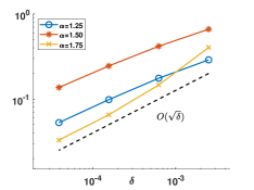
(a) $e_{\text{ini},s}$.

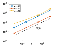
(b) $e_{s}(t)$ with $t=0.5$.

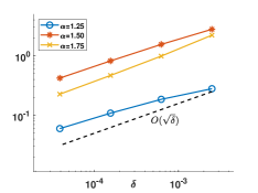
(c) $e_{ini,f}$.

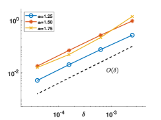
(d) $e_{f}^{n}$ with $t_{n}=0.5$.

Fig. 1: Example (1): semidiscrete errors ((a) and (b)) and fully discrete errors ((c) and (d)). (a): $h=\sqrt{\delta}$ and $\gamma=\sqrt{\delta}/12,\sqrt{\delta},\sqrt{\delta}/2$ for $\alpha=1.25,1.5,1.75$ respectively. (b): $h=\sqrt{\delta}$ and $\gamma=\sqrt{\delta}/5,\sqrt{\delta}/5,\sqrt{\delta}/2$ for $\alpha=1.25,1.5,1.75$respectively. (c): $h=\sqrt{\delta}$, $\tau=\sqrt{\delta}/2$ and $\gamma=\sqrt{\delta}/10$, $\sqrt{\delta}/10$, $\sqrt{\delta}/15$ for $\alpha=1.25,1.5,1.75$ respectively. (d): $h=\sqrt{\delta}$, $\tau=10\delta$ and $\gamma=\delta$, $\delta/2$, $\delta/2$ for $\alpha=1.25,1.5,1.75$ respectively.

By Theorem 15, we compute $\tilde{u}^{\delta}_{h}(0)$ and $\partial_{t}\tilde{u}^{\delta}_{h}(0)$ by choosing the parameters $\gamma\sim\sqrt{\delta}$ and and $h\sim\sqrt{\delta}$ for a given $\delta$, and expect a convergence of order $O(\sqrt{\delta})$. For $t>0$, we compute $\tilde{u}_{h}^{\delta}(t)$ by choosing the parameters $h\sim\sqrt{\delta}$, $\gamma\sim\delta$ for a given $\delta$, and expect a convergence of order $O(\delta)$. In Figure 1 (a) and (b), we plot the errors of semidiscrete solutions with different fractional order $\alpha$. Our numerical experiments fully support our theoretical results in Theorem 15. It is interesting to observe that the error in case of $\alpha=1.5$ is bigger when reconstructing the initial condition, while the error for $\alpha=1.5$ becomes smaller when we compute the solution at time level $t>0$.

Similarly, we compute the numerical solutions to the fully discrete scheme (54) by using the formulae

$$\begin{bmatrix}\tilde{a}_{h,\tau}^{\delta}\\ \tilde{b}_{h,\tau}^{\delta}\end{bmatrix}=\sum_{j=1}^{J}\tilde{\psi}_{\tau}(T_{1},T_{2};\lambda_{j}^{h})^{-1}\begin{bmatrix}\gamma+\bar{F}_{h,\tau}^{N_{2}}&-\bar{F}_{h,\tau}^{N_{1}}\\ -F_{h,\tau}^{N_{2}}&-\gamma+F_{h,\tau}^{N_{1}}\end{bmatrix}\begin{bmatrix}(P_{h}g_{1}^{\delta},\varphi_{j}^{h})\varphi_{j}^{h}\\ (P_{h}g_{2}^{\delta},\varphi_{j}^{h})\varphi_{j}^{h}\end{bmatrix},$$

$$\tilde{U}_{n}^{\delta}=\sum_{j=1}^{J}\tilde{\psi}_{\tau}(T_{1},T_{2};\lambda_{j}^{h})^{-1}\begin{bmatrix}F_{h,\tau}^{n}&\bar{F}_{h,\tau}^{n}\end{bmatrix}\begin{bmatrix}\gamma+\bar{F}_{h,\tau}^{N_{2}}&-\bar{F}_{h,\tau}^{N_{1}}\\ F_{h,\tau}^{N_{2}}&-\gamma+F_{h,\tau}^{N_{1}}\end{bmatrix}\begin{bmatrix}(P_{h}g_{1}^{\delta},\varphi_{j}^{h})\varphi_{j}^{h}\\ (P_{h}g_{2}^{\delta},\varphi_{j}^{h})\varphi_{j}^{h}\end{bmatrix}.$$

Then Theorem 22 implies that for $a,b\in\dot{H}^{2}(\Omega)$

$$\|a_{h,\tau}^{\delta}-a\|_{L^{2}(\Omega)}+\|b_{h,\tau}^{\delta}-b\|_{L^{2}(\Omega)}\leq c(\gamma+\tau+(h^{2}+\delta)\gamma^{-1}),$$

and

$$\|\tilde{U}_{n}^{\delta}-u(t_{n})\|_{L^{2}(\Omega)}\leq c(\gamma+\tau+h^{2}+\delta),\quad\text{for a fixed}~{}~{}t_{n}>0.$$

Therefore, with a given noise level $\delta$, to recover the initial data $a$ and $b$, we choose parameters $h\sim\sqrt{\delta}$, $\tau\sim\sqrt{\delta}$ and $\gamma\sim\sqrt{\delta}$, while to approximate solution $u(t_{n})$ with some $t_{n}>0$, we let $h\sim\sqrt{\delta}$, $\tau\sim\delta$, $\gamma\sim\delta$. According to Theorem 22, we expect that the convergence rate for the error $e_{\text{ini},f}$ is $O(\sqrt{\delta})$ while the error $e_{f}^{n}$ converges to zero as $O(\delta)$ for any fixed $t_{n}>0$. They are fully supported by numerical results plotted in Figure 1 (c) and (d).

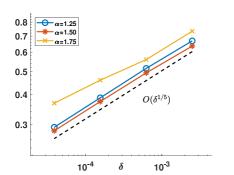
(a) $e_{ini,s}$.

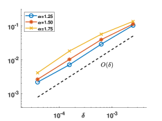
(b) $e_{s}(t)$ with $t=0.5$.

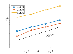
(c) $e_{ini,f}$.

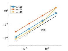
(d) $e^{n}_{f}$ with $t_{n}=0.5$.

Fig. 2: Example (2): semidiscrete errors ((a) and (b)) and fully discrete errors ((c) and (d)). (a): $h=\sqrt{\delta}$ and $\gamma=\delta^{4/5}/15,\delta^{4/5}/15,\delta^{4/5}/8$ for $\alpha=1.25,1.5,1.75$ respectively. (b): $h=\sqrt{\delta}$ and $\gamma=\delta/10,\delta/5,\delta/5$ for $\alpha=1.25,1.5,1.75$ respectively. (c): $h=\sqrt{\delta}$, $\tau=\delta^{1/5}/20$ and $\gamma=\delta^{4/5}/2,\delta^{4/5}/15,\delta^{4/5}/2$ for $\alpha=1.25,1.5,1.75$ respectively. (d): $h=\sqrt{\delta}$, $\tau=10\delta$, $\gamma=\delta/10,\delta,\delta/2$ for $\alpha=1.25,1.5,1.75$ respectively.

Example (2): non-smooth initial data.

Next, we turn to the case of nonsmooth data and expect to examine the influence of weak regularity of problem data. Consider

$$a(x)=\begin{cases}0,\ 0\leq x\leq 0.5;\\ 1,\ 0.5\leq x\leq 1.\end{cases},\quad b(x)=\begin{cases}1,\ 0\leq x\leq 0.5;\\ 0,\ 0.5\leq x\leq 1.\end{cases}$$

and source term $f\equiv 0$. It is well-known that $a,b\in\dot{H}^{\frac{1}{2}-\varepsilon}(\Omega)$ for any $\varepsilon\in(0,\frac{1}{2}]$. According to Theorem 15, the error of the semidiscrete discrete solution satisfies

$$\|\tilde{u}_{h}^{\delta}-a\|_{L^{2}(\Omega)}+\|\partial_{t}\tilde{u}_{h}^{\delta}-b\|_{L^{2}(\Omega)}\leq c(\gamma^{\frac{q}{2}}+(h^{2}+\delta)\gamma^{-1}),$$

$$\|(\tilde{u}_{h}^{\delta}-u)(t)\|_{L^{2}(\Omega)}\leq c(\gamma+h^{2}+\delta),\quad\text{for a given}~{}~{}t>0.$$

Therefore, for given $\delta$, to numerically reconstruct the initial data $a$ and $b$, we let $h=\sqrt{\delta}$, and $\gamma\sim\delta^{4/5}$ and expect that the error converges to zero as $O(\delta^{\frac{1}{5}})$, while to approximate $u(t)$ for some $t>0$, we let $h\sim\sqrt{\delta}$ and $\gamma\sim\delta$ and expect a convergence of order $O(\delta)$. The theoretical results agrees well with the numerical results in Figure 2 (a) and (b).

In Figure 2 (c) and (d) we plot errors of the numerical reconstruction by fully discrete scheme (54). According to Theorem 22 we have the error estimate that (with $q=\frac{1}{2}-\varepsilon$)

$$\|a_{h,\tau}^{\delta}-a\|_{L^{2}(\Omega)}+\|b_{h,\tau}^{\delta}-b\|_{L^{2}(\Omega)}\leq c(\gamma^{\frac{q}{2}}+\tau+(h^{2}+\delta)\gamma^{-1}),$$

$$\|\tilde{U}_{n}^{\delta}-u(t_{n})\|_{L^{2}(\Omega)}\leq c(\gamma+\tau+h^{2}+\delta),\quad\text{for any fixed}~{}~{}t_{n}>0.$$

Therefore we choose parameters $h\sim\sqrt{\delta}$, $\tau\sim\delta^{1/5}$ and $\gamma\sim\delta^{4/5}$ for the numerical reconstruction of initial data, while we let $h\sim\sqrt{\delta}$, $\tau\sim\delta$ and $\gamma\sim\delta$ for approximately solving the solution $u(t_{n})$ for some $t_{n}>0$. The empirical convergence results show that $e_{\text{ini},f}\sim\delta^{\frac{1}{5}}$ and $e_{f}^{n}\sim\delta$, which are consistent with our theoretical findings. Finally, in figure 3, we provide the profiles of solutions to semidiscrete and fully discrete schemes with different noise levels, which show clearly the convergence of the discrete approximation as the noise level $\delta$ decreases.

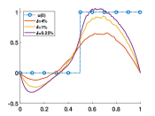
(a) $\tilde{u}^{\delta}_{h}(0)$

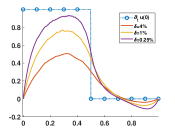
(b) $\partial_{t}\tilde{u}^{\delta}_{h}(0)$

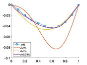
(c) $\tilde{u}^{\delta}_{h}(t)$ with $t=0.5$

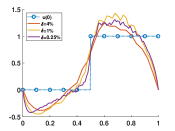
(d) $\tilde{a}_{h,\tau}^{\delta}$

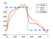
(e) $\tilde{b}_{h,\tau}^{\delta}$

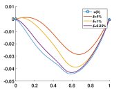
(f) $\tilde{U}_{n}^{\delta}$, with $t_{n}=0.5$

Fig. 3: Example(b): profiles of numerical solutions with $\alpha=1.5$ for $\delta=4\%,1\%,0.25\%$. First row: $h=\sqrt{\delta}/10$, $\gamma=\delta^{4/5}/5$ for both (a) and (b); $h=\sqrt{\delta}/10$, $\gamma=\delta/5$ for (c). Second row: $h=\sqrt{\delta}/10$, $\tau=\delta^{1/5}/10$, $\gamma=\delta^{4/5}/15$ for both (d) and (e); $h=\sqrt{\delta}/10$, $\tau=\delta$, $\gamma=\delta/10$ for (f).

Example (c): 2D examples.

Finally, we test a two dimensional diffusion-wave models in $\Omega=(0,1)^{2}$ with smooth initial conditions:

$$a(x,y)=\sin(2\pi x)\sin(2\pi y),\quad b(x,y)=4x(1-x)y(1-y)\in\dot{H}^{2}(\Omega)=H^{2}(\Omega)\cap H_{0}^{1}(\Omega),$$

and source term $f\equiv 0$. The reference solution is computed with $h=1/150$, $\tau=1/1000$. Noting that the fully discrete system is not symmetric, we apply the biconjugate gradient stabilized method [44].

In Figure 4 and 5, we plot profiles of (numerical) reconstruction of initial data $a$, $b$ and approximation errors, with different noise level $\delta$ as well as different parameters $\gamma,h,\tau$ chosen according to $\delta$. The empirical observations are in excellent agreement with theoretical results, e.g., convergence as the noise level $\delta$ decreases to zero.

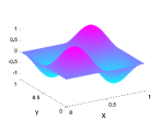
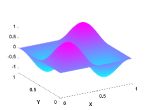
x

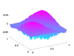
(a) $\delta=1e-2$.

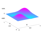
(b) $\delta=5e-3$.

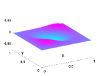
(c) $\delta=2.5e-3$.

Fig. 4: Example(c): Top left: Exact initial data $a$. The remain three columns are profiles of numerical reconstructions $a_{h,\tau}^{\delta}$ and theirs errors, with $h=\sqrt{\delta}/4$, $\tau=\sqrt{\delta}/20$, $\gamma=\sqrt{\delta}/4000$.

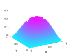
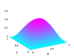
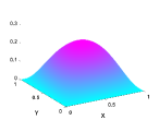
x

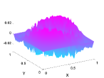
(a) $\delta=1e-2$.

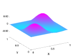
(b) $\delta=5e-3$.

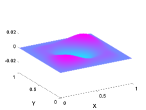
(c) $\delta=2.5e-3$.

Fig. 5: Example(c): Top left: Exact initial data $b$. The remain three columns are profiles of numerical reconstructions $b_{h,\tau}^{\delta}$ and their errors, with $h=\sqrt{\delta}/4$, $\tau=\sqrt{\delta}/20$, $\gamma=\sqrt{\delta}/4000$.

7 Concluding remarks

In this paper, we study the backward diffusion-wave problem, involving a fractional derivative in time with order $\alpha\in(1,2)$. From two terminal observations $u(T_{1})$ and $u(T_{2})$, we simultaneously determine two initial data $u(0)$ and $u_{t}(0)$, as well as the solution $u(t)$ for all $t>0$. The existence, uniqueness and Lipschitz stability of the backward diffusion-wave problem are theoretically examined under some mild conditions on $T_{1}$ and $T_{2}$. Then, in case of noisy observations, we apply quasi-boundary value method to regularize the ”mildly” ill-posed problem, and show the convergence of the regularized solution. Moreover, in order to numerically solve the regularized problem, we proposed a fully discrete scheme by using finite element method in space and convolution quadrature in time. Sharp error bounds of the fully discrete scheme are established in both cases of smooth and nonsmooth data. Numerical experiments fully support our theoretical findings.

Some interesting questions are still open. First of all, we are interested in the fractional evolution model with time-dependent coefficient, e.g.

$$\partial_{t}^{\alpha}u(x,t)+\nabla\cdot(a(x,t)\nabla u)=f(x,t).$$ (62)

The current analysis heavily relies on the decay properties of Mittag–Leffler functions, or equivalently the smoothing properties of solution operators. This stratergy is not directly applicable to the model (62). The direct problem for subdiffusion ($\alpha\in(0,1)$) and its numerical approximation have been studied in [17] by using a perturbation argument. However, the backward problem is still unclear and requires some novel approaches. Besides, we are interested in the backward problem with additional missing information. For example, the inverse source problems, determining source term $f(x)$ and fractional order $\alpha$ from terminal observation $u(T)$, were studied in in [12, 26]. The argument could be extend to the backward problem, but the error analysis of numerical approximation seems more technical.

Appendix A Proof of Lemma 17

Proof.

The estimate for $E_{\alpha,1}(-\lambda t_{n}^{\alpha})-F_{\tau}^{n}(\lambda)$ follows from the same argument in the proof of [51, Lemma 4.2]. Then it suffices to establish a bound for $t_{n}E_{\alpha,2}(-\lambda t^{\alpha})-\bar{F}_{\tau}^{n}(\lambda)$, we recall representations (7) and (49) and derive

$$|t_{n}E_{\alpha,2}(-\lambda t_{n}^{\alpha})-\bar{F}_{\tau}^{n}(\lambda)| \leq\left|\frac{1}{2\pi i}\int_{{\Gamma_{\theta,\sigma}}\backslash{\Gamma_{\theta,\sigma}^{\tau}}}e^{zt_{n}}z^{\alpha-2}(z^{\alpha}+\lambda)^{-1}dz\right|$$

$$\quad+\left|\frac{1}{2\pi i}\int_{\Gamma_{\theta,\sigma}^{\tau}}e^{zt_{n}}(z^{\alpha-2}(z^{\alpha}+\lambda)^{-1}-e^{-z\tau}\delta_{\tau}(e^{-z\tau})^{\alpha-2}(\delta_{\tau}(e^{-z\tau})^{\alpha}+\lambda)^{-1}dz\right|$$

$$:=I_{1}+I_{2}.$$

With $\sigma=t_{n}^{-1}$, the bound for $I_{1}$ follows from the direct computation

$$I_{1} \leq c\int_{{\Gamma_{\theta,\sigma}}\backslash{\Gamma_{\theta,\sigma}^{\tau}}}|e^{zt_{n}}||z^{\alpha-2}||(z^{\alpha}+\lambda)^{-1}||{\rm d}z|\leq c\int_{\pi/(\tau\sin\theta)}^{\infty}\frac{e^{\rho(\cos\theta)t_{n}}\rho^{\alpha-2}}{\rho^{\alpha}}{\rm d}\rho$$

$$\leq ct_{n}\int_{cn}^{\infty}e^{-c\rho}\rho^{-2}{\rm d}\rho\leq ct_{n}n^{-1}$$

and

$$I_{1} \leq c\int_{\pi/(\tau\sin\theta)}^{\infty}\frac{e^{\rho(\cos\theta)t_{n}}\rho^{\alpha-2}}{\lambda}{\rm d}\rho\leq ct_{n}(\lambda t_{n}^{\alpha})^{-1}\int_{cn}^{\infty}e^{-c\rho}\rho^{\alpha-2}d\rho$$

$$\leq ct_{n}(\lambda t_{n}^{\alpha})^{-1}n^{-1}\int_{cn}^{\infty}e^{-c\rho}\rho^{\alpha-1}d\rho\leq ct_{n}(\lambda t_{n}^{\alpha})^{-1}n^{-1}.$$

As a result, we obtain $I_{1}\leq\frac{cn^{-1}}{(1+\lambda t_{n}^{\alpha})}t_{n}.$ Next we turn to the term $I_{2}$. According to Lemma 16, we have for all $z\in{\Gamma_{\theta,\sigma}^{\tau}}$,

$$\left|\frac{z^{\alpha-2}}{z^{\alpha}+\lambda}-\frac{e^{-z\tau}\delta_{\tau}(e^{-z\tau})^{\alpha-2}}{\delta_{\tau}(e^{-z\tau})^{\alpha}+\lambda}\right| \leq c\tau\frac{|z|^{\alpha-1}}{|z^{\alpha}+\lambda|}$$

Therefore, with $\sigma=t_{n}^{-1}$, the term $I_{2}$ can be bounded as

$$I_{2} \leq c\tau\int_{\Gamma_{\theta,\sigma}^{\tau}}|e^{zt_{n}}|\frac{|z|^{\alpha-1}}{|z^{\alpha}+\lambda|}|dz|\leq c\tau\lambda^{-1}(\int_{\sigma}^{\infty}e^{\rho\cos\theta t_{n}}\rho^{\alpha-1}d\rho+\sigma^{\alpha}\int_{-\theta}^{\theta}d\psi)\leq c\tau(\lambda t_{n}^{\alpha})^{-1}$$

and

$$I_{2} \leq c\tau\int_{\Gamma_{\theta,\sigma}^{\tau}}|e^{zt_{n}}||z|^{-1}|dz|\leq c\tau(\int_{1}^{\infty}e^{\rho\cos\theta}\rho^{-1}d\rho+\int_{-\theta}^{\theta}d\psi)\leq c\tau.$$

Then (50) follows immediately.

For the second estimate, we note that

$$t_{n}E_{\alpha,2}(-\lambda t_{n}^{\alpha}) =t_{n}-\frac{\lambda}{2\pi i}\int_{\Gamma_{\theta,\sigma}}e^{zt_{n}}z^{-2}(z^{\alpha}+\lambda)^{-1}dz,$$

$$\bar{F}_{\tau}^{n}(\lambda) =t_{n}-\frac{\lambda}{2\pi i}\int_{\Gamma_{\theta,\sigma}^{\tau}}e^{zt_{n}}e^{-z\tau}\delta_{\tau}(e^{-z\tau})^{-2}(\delta_{\tau}(e^{-z\tau})^{\alpha}+\lambda)^{-1}dz,$$

with $n\geq 1$. Then we use the spliiting

$$\lambda^{-1}|t_{n}E_{\alpha,2}(-\lambda t_{n}^{\alpha})-\bar{F}_{\tau}^{n}(\lambda)| \leq\left|\frac{1}{2\pi i}\int_{{\Gamma_{\theta,\sigma}}\backslash{\Gamma_{\theta,\sigma}^{\tau}}}e^{zt_{n}}z^{-2}(z^{\alpha}+\lambda)^{-1}dz\right|$$

$$+\left|\frac{1}{2\pi i}\int_{{\Gamma_{\theta,\sigma}^{\tau}}}e^{zt_{n}}[z^{-2}(z^{\alpha}+\lambda)^{-1}-e^{-z\tau}\delta_{\tau}(e^{-z\tau})^{-2}(\delta_{\tau}(e^{-z\tau})^{\alpha}+\lambda)^{-1}]dz\right|$$

$$:=I_{1}+I_{2}.$$

According to Lemma 16 we have for all $z\in\Gamma_{\theta,\sigma}^{\tau}$ ,

$$I_{1} \leq c\int_{{\Gamma_{\theta,\sigma}}\backslash{\Gamma_{\theta,\sigma}^{\tau}}}|e^{zt_{n}}||z|^{-\alpha-2}|dz|\leq c\int_{\pi/(\tau\sin\theta)}e^{\rho\cos\theta t_{n}}\rho^{-\alpha-2}d\rho$$

$$\leq ct_{n}^{\alpha+1}\int_{cn}^{\infty}e^{-c\rho}\rho^{-\alpha-2}d\rho\leq ct_{n}^{\alpha+1}n^{-3}\int_{0}^{\infty}e^{-c\rho}\rho^{-\alpha+1}d\rho\leq ct_{n}^{\alpha-2}\tau^{3}.$$

And also we have

$$|z^{-2}(z^{\alpha}+\lambda)^{-1}-e^{-z\tau}\delta_{\tau}(e^{-z\tau})^{-2}(\delta_{\tau}(e^{-z\tau})^{\alpha}+\lambda)^{-1}|\leq c\tau|z|^{-\alpha-1},$$

and therefore with $\sigma=t_{n}^{-1}$, we have the bound for $n\geq 1$

$$I_{2} \leq c\tau\int_{\Gamma_{\theta,\sigma}^{\tau}}|e^{zt_{n}}||z|^{-\alpha-1}|dz|\leq c\tau\left(\int_{\sigma}^{\infty}e^{-c\rho t_{n}}\rho^{-\alpha-1}d\rho+\sigma^{-\alpha}\int_{-\theta}^{\theta}d\psi\right)\leq c\tau t_{n}^{\alpha}.$$

This completes the proof of (51). ∎

References

- [1] E. E. Adams and L. W. Gelhar. Field study of dispersion in a heterogeneous aquifer: 2. spatial moments analysis. Water Res. Research, 28(12):3293–3307, 1992.
- [2] D. Baffet and J. S. Hesthaven. A kernel compression scheme for fractional differential equations. SIAM J. Numer. Anal., 55(2):496–520, 2017.
- [3] E. G. Bajlekova. Fractional Evolution Equations in Banach Spaces. PhD thesis, Eindhoven University of Technology, 2001.
- [4] L. Banjai and M. López-Fernández. Efficient high order algorithms for fractional integrals and fractional differential equations. Numer. Math., 141(2):289–317, 2019.
- [5] S. Chen, J. Shen, Z. Zhang, and Z. Zhou. A spectrally accurate approximation to subdiffusion equations using the log orthogonal functions. SIAM J. Sci. Comput., 42(2):A849–A877, 2020.
- [6] E. Cuesta, C. Lubich, and C. Palencia. Convolution quadrature time discretization of fractional diffusion-wave equations. Math. Comp., 75(254):673–696, 2006.
- [7] M. Fischer. Fast and parallel Runge-Kutta approximation of fractional evolution equations. SIAM J. Sci. Comput., 41(2):A927–A947, 2019.
- [8] G. Floridia and M. Yamamoto. Backward problems in time for fractional diffusion-wave equation. Inverse Problems, 36(12):125016, 14, 2020.
- [9] D. N. Hào, J. Liu, N. V. Duc, and N. V. Thang. Stability results for backward time-fractional parabolic equations. Inverse Problems, 35(12):125006, 25, 2019.
- [10] Y. Hatano and N. Hatano. Dispersive transport of ions in column experiments: An explanation of long-tailed profiles. Water Res. Research, 34(5):1027–1033, 1998.
- [11] D. Hou and C. Xu. A fractional spectral method with applications to some singular problems. Adv. Comput. Math., 43(5):911–944, 2017.
- [12] J. Janno and N. Kinash. Reconstruction of an order of derivative and a source term in a fractional diffusion equation from final measurements. Inverse Problems, 34(2):025007, 19, 2018.
- [13] S. Jiang, J. Zhang, Q. Zhang, and Z. Zhang. Fast evaluation of the Caputo fractional derivative and its applications to fractional diffusion equations. Commun. Comput. Phys., 21(3):650–678, 2017.
- [14] B. Jin. Fractional differential equations—an approach via fractional derivatives, volume 206 of Applied Mathematical Sciences. Springer, Cham, [2021] ©2021.
- [15] B. Jin, R. Lazarov, and Z. Zhou. Two fully discrete schemes for fractional diffusion and diffusion-wave equations with nonsmooth data. SIAM J. Sci. Comput., 38(1):A146–A170, 2016.
- [16] B. Jin, B. Li, and Z. Zhou. Correction of high-order BDF convolution quadrature for fractional evolution equations. SIAM J. Sci. Comput., 39(6):A3129–A3152, 2017.
- [17] B. Jin, B. Li, and Z. Zhou. Subdiffusion with a time-dependent coefficient: analysis and numerical solution. Math. Comp., 88(319):2157–2186, 2019.
- [18] B. Jin and W. Rundell. A tutorial on inverse problems for anomalous diffusion processes. Inverse Problems, 31(3):035003, 40, 2015.
- [19] A. A. Kilbas, H. M. Srivastava, and J. J. Trujillo. Theory and Applications of Fractional Differential Equations. Elsevier Science B.V., Amsterdam, 2006.
- [20] N. Kopteva. Error analysis of an L2-type method on graded meshes for a fractional-order parabolic problem. Preprint, arXiv:1905.05070, 2019.
- [21] N. Kopteva. Error analysis for time-fractional semilinear parabolic equations using upper and lower solutions. SIAM J. Numer. Anal., 58(4):2212–2234, 2020.
- [22] N. Kopteva. Error analysis of an L2-type method on graded meshes for a fractional-order parabolic problem. Math. Comp., 90(327):19–40, 2021.
- [23] Z. Li, Y. Liu, and M. Yamamoto. Inverse problems of determining parameters of the fractional partial differential equations. In Handbook of fractional calculus with applications. Vol. 2, pages 431–442. De Gruyter, Berlin, 2019.
- [24] Z. Li and M. Yamamoto. Inverse problems of determining coefficients of the fractional partial differential equations. In Handbook of fractional calculus with applications. Vol. 2, pages 443–464. De Gruyter, Berlin, 2019.
- [25] H.-l. Liao, D. Li, and J. Zhang. Sharp error estimate of the nonuniform L1 formula for linear reaction-subdiffusion equations. SIAM J. Numer. Anal., 56(2):1112–1133, 2018.
- [26] K. Liao and T. Wei. Identifying a fractional order and a space source term in a time-fractional diffusion-wave equation simultaneously. Inverse Problems, 35(11):115002, 23, 2019.
- [27] J. J. Liu and M. Yamamoto. A backward problem for the time-fractional diffusion equation. Appl. Anal., 89(11):1769–1788, 2010.
- [28] Y. Liu, Z. Li, and M. Yamamoto. Inverse problems of determining sources of the fractional partial differential equations. In Handbook of fractional calculus with applications. Vol. 2, pages 411–429. De Gruyter, Berlin, 2019.
- [29] M. López-Fernández, C. Lubich, and A. Schädle. Adaptive, fast, and oblivious convolution in evolution equations with memory. SIAM J. Sci. Comput., 30(2):1015–1037, 2008.
- [30] C. Lubich. Discretized fractional calculus. SIAM J. Math. Anal., 17(3):704–719, 1986.
- [31] F. Mainardi. Fractional relaxation-oscillation and fractional diffusion-wave phenomena. Chaos Solitons Fractals, 7(9):1461–1477, 1996.
- [32] F. Mainardi. Fractional calculus and waves in linear viscoelasticity. Imperial College Press, London, 2010. An introduction to mathematical models.
- [33] W. McLean and K. Mustapha. Time-stepping error bounds for fractional diffusion problems with non-smooth initial data. J. Comput. Phys., 293:201–217, 2015.
- [34] R. Metzler, J.-H. Jeon, A. G. Cherstvy, and E. Barkai. Anomalous diffusion models and their properties: non-stationarity, non-ergodicity, and ageing at the centenary of single particle tracking. Phys. Chem. Chem. Phys., 16:24128, 37 pp., 2014.
- [35] R. Metzler and J. Klafter. The random walk’s guide to anomalous diffusion: a fractional dynamics approach. Phys. Rep., 339(1):1–77, 2000.
- [36] K. Mustapha, B. Abdallah, and K. M. Furati. A discontinuous Petrov-Galerkin method for time-fractional diffusion equations. SIAM J. Numer. Anal., 52(5):2512–2529, 2014.
- [37] R. Nigmatullin. The realization of the generalized transfer equation in a medium with fractal geometry. Phys. Stat. Sol. B, 133(1):425–430, 1986.
- [38] I. Podlubny. Fractional differential equations : an introduction to fractional derivatives, fractional differential equations, to methods of their solution and some of their applications. Academic Press, San Diego, 1999.
- [39] K. Sakamoto and M. Yamamoto. Initial value/boundary value problems for fractional diffusion-wave equations and applications to some inverse problems. J. Math. Anal. Appl., 382(1):426–447, 2011.
- [40] H. Seybold and R. Hilfer. Numerical algorithm for calculating the generalized Mittag-Leffler function. SIAM J. Numer. Anal., 47(1):69–88, 2008/09.
- [41] M. Stynes, E. O’Riordan, and J. L. Gracia. Error analysis of a finite difference method on graded meshes for a time-fractional diffusion equation. SIAM J. Numer. Anal., 55(2):1057–1079, 2017.
- [42] V. Thomée. Galerkin Finite Element Methods for Parabolic Problems. Springer-Verlag, Berlin, 2nd edition, 2006.
- [43] N. H. Tuan, T. B. Ngoc, Y. Zhou, and D. O’Regan. On existence and regularity of a terminal value problem for the time fractional diffusion equation. Inverse Problems, 36(5):055011, 41, 2020.
- [44] H. A. van der Vorst. Bi-CGSTAB: A fast and smoothly converging variant of bi-CG for the solution of nonsymmetric linear systems. SIAM Journal on Scientific and Statistical Computing, 13(2):631–644, mar 1992.
- [45] L. Wang and J. Liu. Total variation regularization for a backward time-fractional diffusion problem. Inverse Problems, 29(11):115013, 22, 2013.
- [46] T. Wei and J.-G. Wang. A modified quasi-boundary value method for the backward time-fractional diffusion problem. ESAIM Math. Model. Numer. Anal., 48(2):603–621, 2014.
- [47] T. Wei and Y. Zhang. The backward problem for a time-fractional diffusion-wave equation in a bounded domain. Comput. Math. Appl., 75(10):3632–3648, 2018.
- [48] Q. Xu, J. S. Hesthaven, and F. Chen. A parareal method for time-fractional differential equations. J. Comput. Phys., 293:173–183, 2015.
- [49] M. Yang and J. Liu. Solving a final value fractional diffusion problem by boundary condition regularization. Appl. Numer. Math., 66:45–58, 2013.
- [50] M. Zayernouri and G. E. Karniadakis. Fractional Sturm-Liouville eigen-problems: theory and numerical approximation. J. Comput. Phys., 252:495–517, 2013.
- [51] Z. Zhang and Z. Zhou. Numerical analysis of backward subdiffusion problems. Inverse Problems, 36(10):105006, oct 2020.
- [52] H. Zhu and C. Xu. A fast high order method for the time-fractional diffusion equation. SIAM J. Numer. Anal., 57(6):2829–2849, 2019.