Automatic Symmetry Discovery with Lie Algebra Convolutional Network

Abstract

Existing equivariant neural networks require prior knowledge of the symmetry group and discretization for continuous groups. We propose to work with Lie algebras (infinitesimal generators) instead of Lie groups. Our model, the Lie algebra convolutional network (L-conv) can automatically discover symmetries and does not require discretization of the group. We show that L-conv can serve as a building block to construct any group equivariant feedforward architecture. Both CNNs and Graph Convolutional Networks can be expressed as L-conv with appropriate groups. We discover direct connections between L-conv and physics: (1) group invariant loss generalizes field theory (2) Euler-Lagrange equation measures the robustness, and (3) equivariance leads to conservation laws and Noether current. These connections open up new avenues for designing more general equivariant networks and applying them to important problems in physical sciences.

1 Introduction

Incorporating symmetries into a deep learning architecture can reduce sample complexity, improve generalization, while significantly decreasing the number of model parameters (Cohen et al., 2019b; Cohen & Welling, 2016b; Ravanbakhsh et al., 2017; Ravanbakhsh, 2020; Wang et al., 2020). For instance, Convolutional Neural Networks (CNN) (LeCun et al., 1989, 1998) implement translation symmetry through weight sharing. General principles for constructing symmetry-aware group equivariant neural networks were introduced in Cohen & Welling (2016b), Kondor & Trivedi (2018), and Cohen et al. (2019b).

However, most work on equivariant networks requires knowing the symmetry group a priori. A different equivariant model needs to be re-designed for each symmetry group. In practice, we may not have a good inductive bias and such knowledge of the symmetries may not be available. Constructing and selecting the equivariant network with the appropriate symmetry group becomes quite tedious. Furthermore, many existing works are limited to finite groups such as permutations Hartford et al. (2018); Ravanbakhsh et al. (2017); Zaheer et al. (2017), $90$ degree rotations Cohen et al. (2018) or dihedral groups $\mathrm{D}_{N}$ $E(2)$ Weiler & Cesa (2019).

For a continuous group, existing approaches either discretize the group Weiler et al. (2018a, b); Cohen & Welling (2016a), or use a truncated sum over irreducible representations (irreps) Weiler & Cesa (2019); Weiler et al. (2018a) via spherical harmonics in Worrall et al. (2017) or more general Clebsch-Gordon coefficients Kondor et al. (2018); Bogatskiy et al. (2020). These approaches are prone to approximation error. Recently, Finzi et al. (2020) propose to approximates the integral over the Lie group by Monte Carlo sampling. This approach requires implementing the matrix exponential and obtaining a local neighborhood for each point. Both parametrizing Lie groups for sampling and finding irreps are computationally expensive. Finzi et al. (2021) provide a general algorithm for constructing equivariant multi-layer perceptrons (MLP), but require explicit knowledge of the group to encode its irreps, and solving a set of constraints.

We provide a novel framework for designing equivariant neural networks. We leverage the fact that Lie groups can be constructed from a set of infinitesimal generators, called Lie algebras. A Lie algebra has a finite basis, assuming the group is finite-dimensional. Working with the Lie algebra basis allows us to encode an infinite group without discretizing or summing over irreps. Additionally, all Lie algebras have the same general structure and hence can be implemented the same way. We propose Lie Algebra Convolutional Network (L-conv), a novel architecture that can automatically discover symmetries from data. Our main contributions can be summarized as follows:

• We propose the Lie algebra convolutional network (L-conv), a building block for constructing group equivariant neural networks.

• We prove that multi-layer L-conv can approximate group convolutional layers, including CNNs, and find graph convolutional networks to be a special case of L-conv.

• We can learn the Lie algebra basis in L-conv, enabling automatic symmetry discovery.

• L-conv also reveals interesting connections between physics and learning: equivariant loss generalizes important Lagrangians in field theory; robustness and equivariance can be expressed as Euler-Lagrange equations and Noether currents.

Learning symmetries from data has been studied in limited settings for commutative Lie groups as in Cohen & Welling (2014), 2D rotations and translations in Rao & Ruderman (1999), Sohl-Dickstein et al. (2010) or permutations (Anselmi et al., 2019). (Zhou et al., 2020) popose a general method for symmetry discovery. Yet, their weight-sharing scheme and the symmetry generators are very different from ours. Our approach use much fewer parameters and has a direct interpretation using Lie algebras (SI B.3). Benton et al. (2020) propose Augerino to learn a distribution over data augmentations. It also involves Lie algebras, but is restricted to a subgroup of 2D affine transformations and requires matrix logarithm and sampling (SI B.3). In contrast, our approach is simpler and more general.

2 Background

We review the core concepts L-conv builds upon: equivariance, group convolution and Lie algebras.

Notations. Unless explicitly stated, $a$ in $A^{a}$ is an index, not an exponent. We use the Einstein summation $A^{a}B_{ab}=\sum_{a}A^{a}B_{ab}=[AB]_{b}$, where a repeated upper and lower index are summed.

Equivariance. Let $\mathcal{S}$ be a topological space on which a Lie group $G$ (continuous group) acts from the left, meaning for all ${\bm{x}}\in\mathcal{S}$ and $g\in G$, $g{\bm{x}}\in\mathcal{S}$. We refer to $\mathcal{S}$ as the base space. Let $\mathcal{F}$, the “feature space”, be the vector space $\mathcal{F}=\mathbb{R}^{m}$. Each data point is a feature map $f:\mathcal{S}\to\mathcal{F}$. The action of $G$ on the input of $f$ induces an action on feature maps. For “scalar” features, for $u\in G$, the transformed features $u\cdot f$ are given by

$$u\cdot f({\bm{x}}) =f(u^{-1}{\bm{x}}).$$ (1)

Denote the space of all functions from $\mathcal{S}$ to $\mathcal{F}$ by $\mathcal{F}^{\mathcal{S}}$, so that $f\in\mathcal{F}^{\mathcal{S}}$. Let $F$ be a mapping to a new feature space $\mathcal{F}^{\prime}=\mathbb{R}^{m^{\prime}}$, meaning $F:\mathcal{F}^{\mathcal{S}}\to{\mathcal{F}^{\prime}}^{\mathcal{S}}$. We say $F$ is equivariant under $G$ if $G$ acts on $\mathcal{F}^{\prime}$ and for $u\in G$, we have

$$u\cdot(F(f)) =F(u\cdot f).$$ (2)

Group Convolution. Kondor & Trivedi (2018) showed that $F$ is a linear equivariant map if and only if it performs a group convolution (G-conv). To define G-conv, we first lift ${\bm{x}}$ to elements in $G$ (Kondor & Trivedi, 2018). Specifically, we pick an origin ${\bm{x}}_{0}\in\mathcal{S}$ and replace each point ${\bm{x}}=g{\bm{x}}_{0}$ by $g$. We will often drop ${\bm{x}}_{0}$ for brevity and write $f(g)\equiv f(g{\bm{x}}_{0})$. Let $\kappa:G\to\mathbb{R}^{m^{\prime}}\otimes\mathbb{R}^{m}$ be a linear transformation from $\mathcal{F}$ to $\mathcal{F}^{\prime}$. G-conv is defined as

$$[\kappa\star f](g)=\int_{G}\kappa(g^{-1}v)f(v)dv=\int_{G}\kappa(v)f(gv)dv,$$ (3)

We denote the Haar measure on $G$ as $dv\equiv d\mu(v)$ for brevity.

Equivariance of G-conv. G-conv in equation 3 is equivariant (Kondor & Trivedi, 2018). By definition, for $w\in G$ we have

$$[\kappa\star w\cdot f](g) =\int_{G}\kappa(v)w\cdot f(gv)dv=\int_{G}\kappa(v)f(w^{-1}gv)dv$$ (4)

$$=[\kappa\star f](w^{-1}g)=w\cdot[\kappa\star f](g)$$ (5)

Existing works on equivariance networks implement $\int_{G}$ by discretizing the group or summing over irreps. We take a different approach and use the infinitesimal generators of the group. While a Lie group $G$ is infinite, usually it can be generated using a small number of infinitesimal generator, comprising its “Lie algebra”. We use the Lie algebra to introduce a building block to approximate G-conv. Figure 1 visualizes a Lie group, Lie algebra and the concept we discuss below.

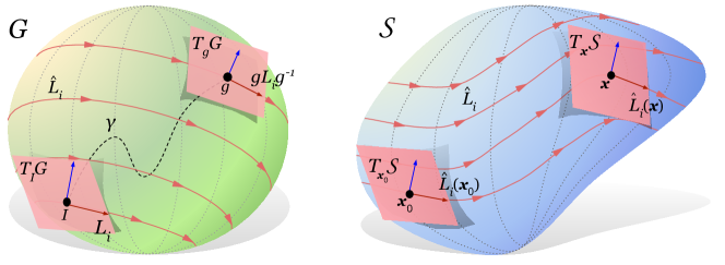
Figure 1: Lie group and Lie algebra: Illustration of the group manifold of a Lie group $G$ (left). The Lie algebra $\mathfrak{g}=T_{I}G$ is the tangent space at the identity $I$. $L_{i}$ are a basis for $T_{I}G$. If $G$ is connected, $\forall g\in G$ there exist paths like $\gamma$ from $I$ to $g$ and $g$ can be written as a path-ordered integral $g=P\exp[\int_{\gamma}dt^{i}L_{i}]$. Base space Right is a schematic of the base space $\mathcal{S}$ as a manifold. The lift ${\bm{x}}=g{\bm{x}}_{0}$ takes ${\bm{x}}\in\mathcal{S}$ to $g\in G$, and maps the tangent spaces $T_{\bm{x}}\mathcal{S}\to T_{g}G$. Each Lie algebra basis $L_{i}\in\mathfrak{g}=T_{I}G$ generates a vector field $\hat{L}_{i}$ on the tangent bundle $TG$ via the pushforward $\hat{L}_{i}(g)=gL_{i}g^{-1}$. Via the lift, $L_{i}$ also generates a vector field $\hat{L}_{i}=\hat{L}_{i}^{\alpha}({\bm{x}})\partial_{\alpha}=[gL_{i}{\bm{x}}_{0}]^{\alpha}\partial_{\alpha}$.

Lie algebra. Let $G$ be a Lie group, which includes common continuous groups. Group elements $u\in G$ infinitesimally close to the identity element $I$ can be written as $u\approx I+{\epsilon}^{i}L_{i}$ (note Einstein summation), where $L_{i}\in\mathfrak{g}$ with the Lie algebra $\mathfrak{g}=T_{I}G$ is the tangent space of $G$ at the identity element. The Lie algebra has the property that it is closed under a Lie bracket $[\cdot,\cdot]:\mathfrak{g}\times\mathfrak{g}\to\mathfrak{g}$

$$[L_{i},L_{j}] ={c_{ij}}^{k}L_{k},$$ (6)

which is skew-symmetric and satisfies the Jacobi identity. Here the coefficients ${c_{ij}}^{k}\in\mathbb{R}$ or $\mathbb{C}$ are called the structure constants of the Lie algebra. For matrix representations of $\mathfrak{g}$, $[L_{i},L_{j}]=L_{i}L_{j}-L_{j}L_{i}$ is the commutator. The $L_{i}$ are called the infinitesimal generators of the Lie group.

Exponential map. If the manifold of $G$ is connected , an exponential map $\exp:\mathfrak{g}\to G$ can be defined such that $g=\exp[t^{i}L_{i}]\in G$. For matrix groups, if $G$ is connected and compact, the matrix exponential is such a map and it is surjective. For most other groups (except $\mathrm{GL}_{d}(\mathbb{C})$ and nilpotent groups) it is not surjective. Nevertheless, for any connected group every $g\in G$ can be written as a product $g=\prod_{a}\exp[t_{a}^{i}L_{i}]$ (Hall, 2015). Making $t^{i}_{a}$ infinitesimal steps $dt^{i}(s)$ tangent to a path $\gamma$ from $I$ to $g$ on $G$ yields the surjective path-ordered exponential in physics, denoted as $g=P\exp[\int_{\gamma}dt^{i}L_{i}]$ (SI A, and see Time-ordering in Weinberg (1995, p143)).

Pushforward. $L_{i}\in T_{I}G$ can be pushed forward to $\hat{L}_{i}(g)=gL_{i}g^{-1}\in T_{g}G$ to form a basis for $T_{g}G$, satisfying the same Lie algebra $[\hat{L}_{i}(g),\hat{L}_{j}(g)]={c_{ij}}^{k}\hat{L}_{k}(g)$. The manifold of $G$ together with the set of all $T_{g}G$ attached to each $g$ forms the tangent bundle $TG$, a type of fiber bundle (Lee et al., 2009). $\hat{L}_{i}$ is a vector field on $TG$. The lift maps $\hat{L}_{i}$ to an equivalent vector field on $T\mathcal{S}$, which we will also denote by $\hat{L}_{i}$. Figure 1 illustrates the flow of these vector fields on $TG$ and $T\mathcal{S}$.

3 Lie Algebra Convolutional Network

We can use the Lie algebra basis $L_{i}\in\mathfrak{g}$ to construct the Lie group $G$ with the exponential map. Similarly, we show that Lie algebras can also serve as building blocks to construct G-conv layers. We propose the Lie algebra convolutional network (L-conv). The key idea is to approximate the kernel $\kappa(u)$ using localized kernels which can be constructed using the Lie algebra (Fig. 2). This is possible because the exponential map is a generalization of a Taylor expansion. We show that a G-conv whose kernel is concentrated near the identity can be expanded in the Lie algebra.

Let $\delta_{\eta}(u)\in\mathbb{R}$ denote a normalized localized kernel, meaning $\int_{G}\delta_{\eta}(g)dg=1$, and with support on a small neighborhood of size $\eta$ near the identity $I$ (i.e., $\delta_{\eta}(I+{\epsilon}^{i}L_{i})\to 0$ if $\|{\epsilon}\|^{2}>\eta^{2}$). Let $\kappa_{0}(u)=W^{0}\delta_{\eta}(u)$, where $W^{0}\in\mathbb{R}^{m^{\prime}}\otimes\mathbb{R}^{m}$ are constants. The localized kernels $\kappa_{0}$ can be used to approximate G-conv. We first derive the expression for a G-conv whose kernel is $\kappa_{0}$.

Linear expansion of G-conv with localized kernel. We can expand a G-conv whose kernel is $\kappa_{0}(u)=W^{0}\delta_{\eta}(u)$ in the Lie algebra of $G$ to linear order. With $v_{\epsilon}=I+{\epsilon}^{i}L_{i}$, we have (see SI A)

$$Q[f](g) =[\kappa_{0}\star f](g)=\int_{G}dv\kappa_{0}(v)f(gv)=\int_{\|{\epsilon}\|<\eta}dv_{\epsilon}\kappa_{0}(v_{\epsilon})f(gv_{\epsilon})$$ (7)

$$=W^{0}\int d{\epsilon}\delta_{\eta}(v_{\epsilon})\left[f(g)+{\epsilon}^{i}gL_{i}\cdot{d\over dg}f(g)+O({\epsilon}^{2})\right]$$ (8)

$$=W^{0}\left[I+\overline{{\epsilon}}^{i}gL_{i}\cdot{d\over dg}\right]f(g)+O(\eta^{2})$$ (9)

where $W^{0}\in\mathbb{R}^{m^{\prime}}\otimes\mathbb{R}^{m}$, and using $\int_{G}\delta_{\eta}(g)dg=\int d{\epsilon}\delta_{\eta}(v_{\epsilon})=1$ and ${\epsilon}^{i}\in\mathbb{R}^{m}\otimes\mathbb{R}^{m}$, we defined

$$\overline{{\epsilon}}^{i} =\int d{\epsilon}\delta_{\eta}(v_{\epsilon}){\epsilon}^{i}\in\mathbb{R}^{m}\otimes\mathbb{R}^{m}.$$ (10)

Note that because $\|{\epsilon}\|<\eta$ we also have $\|\overline{{\epsilon}}\|<\eta$ (SI A, equation 38). Here $d{\epsilon}$ is the integration measure on the Lie algebra $\mathfrak{g}=T_{I}G$ induced by the Haar measure $dv_{\epsilon}$ on $G$.

Interpreting the derivatives. In a matrix representation of $G$, we have $gL_{i}\cdot{df\over dg}=[gL_{i}]_{\alpha}^{\beta}{df\over dg_{\alpha}^{\beta}}=\mathrm{Tr}\left[[gL_{i}]^{T}{df\over dg}\right]$. This can be written in terms of partial derivatives $\partial_{\alpha}f({\bm{x}})=\partial f/\partial{\bm{x}}^{\alpha}$ as follows. Using ${\bm{x}}^{\rho}=g^{\rho}_{\sigma}{\bm{x}}_{0}^{\sigma}$, we have ${df(g{\bm{x}}_{0})\over dg^{\alpha}_{\beta}}={\bm{x}}_{0}^{\beta}\partial_{\alpha}f({\bm{x}})$, and so

$$\hat{L}_{i}f({\bm{x}})\equiv gL_{i}\cdot{df\over dg} =[gL_{i}]^{\alpha}_{\beta}{\bm{x}}_{0}^{\beta}\partial_{\alpha}f({\bm{x}})=[gL_{i}{\bm{x}}_{0}]\cdot\nabla f({\bm{x}})$$ (11)

Hence, for each $L_{i}$, the pushforward $gL_{i}g^{-1}$ generates a flow on $\mathcal{S}$ through the vector field $\hat{L}_{i}\equiv gL_{i}\cdot d/dg=[gL_{i}g^{-1}{\bm{x}}]^{\alpha}\partial_{\alpha}$ (Fig. 1).

Lie algebra convolutional (L-conv) layer. Equation 9 states that for a kernel localized near the identity, the effect of the kernel can be summarized in $W^{0}$ and $\overline{{\epsilon}}^{i}\hat{L}_{i}$. Note that we do not need to perform the integral over $G$ explicitly anymore. Instead of working with a kernel $\kappa_{0}$, we only need to specify $W^{0}$ and $\overline{{\epsilon}}^{i}$. Hence, in general, we define the Lie algebra convolution (L-conv) as

$$Q[f]({\bm{x}}) =W^{0}\left[I+\overline{{\epsilon}}^{i}\hat{L}_{i}\right]f({\bm{x}})$$ (12)

$$=W^{0}\left[I+\overline{{\epsilon}}^{i}[gL_{i}{\bm{x}}_{0}]^{\alpha}\partial_{\alpha}\right]f({\bm{x}})$$ (13)

Being an expansion of G-conv, L-conv inherits the equivariance of G-conv, as we show next.

Proposition 1 (Equivariance of L-conv).

With assumptions above, L-conv is equivariant under $G$.

Proof: First, note that the components of $\hat{L}_{i}$ transform as $[\hat{L}_{i}(v{\bm{x}})]^{\alpha}=[vgL_{i}{\bm{x}}_{0}]^{\alpha}=v^{\alpha}_{\beta}\hat{L}_{i}({\bm{x}})^{\beta}$, while the partial transforms as $\partial/\partial[v{\bm{x}}]^{\alpha}=[v^{-1}]^{\gamma}_{\alpha}\partial_{\gamma}$. As a result in $\hat{L}_{i}=[gL_{i}{\bm{x}}_{0}]^{\alpha}\partial_{\alpha}$ all factors of $v$ cancel, meaning for $v\in G$, $\hat{L}_{i}(v{\bm{x}})=\hat{L}_{i}({\bm{x}})$. This is because of the fact that $\hat{L}_{i}\in T\mathcal{S}$ is a vector field (i.e. 1-tensor) and, thus, invariant under change of basis. Plugging into equation 13, for $w\in G$

$$w\cdot Q[f]({\bm{x}}) =Q[f](w^{-1}{\bm{x}})=W^{0}\left[I+\overline{{\epsilon}}^{i}\hat{L}_{i}(w^{-1}{\bm{x}})\right]f(w^{-1}{\bm{x}})$$ (14)

$$=W^{0}\left[I+\overline{{\epsilon}}^{i}\hat{L}_{i}(g)\right]f(w^{-1}{\bm{x}})=W^{0}\left[I+\overline{{\epsilon}}^{i}\hat{L}_{i}(g)\right]w\cdot f({\bm{x}})=Q[w\cdot f]({\bm{x}})$$ (15)

which proves L-conv is equivariant. $\square$

Examples. Using equation 11 we can calculate L-conv for specific groups (details in SI A.2). For translations $G=T_{n}=(\mathbb{R}^{n},+)$, we find the generators become simple partial derivatives $\hat{L}_{i}=\partial_{i}$ (SI A.2.2), yielding $f({\bm{x}})+{\epsilon}^{\alpha}\partial_{\alpha}f({\bm{x}})$. For 2D rotations (SI A.2.1) the generator $\hat{L}\equiv\left(x\partial_{y}-y\partial_{x}\right)=\partial_{\theta}$, which is the angular momentum operator about the z-axis in quantum mechanics and field theories. For rotations with scaling, $G=SO(2)\times\mathbb{R}^{+}$, we have two $L_{i}$, one $\hat{L}_{\theta}=\partial_{\theta}$ from $so(2)$ and a scaling with $L_{r}=I$, yielding $\hat{L}_{r}=x\partial_{x}+y\partial_{y}=r\partial_{r}$. Next, we discuss the form of L-conv on discrete data.

3.1 Approximating G-conv using L-conv

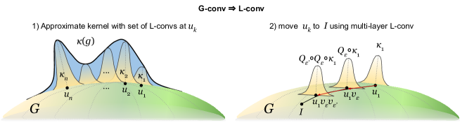
Figure 2: Sketch of the procedure for approximating G-conv using L-conv. First, the kernel is written as the sum of a number of localized kernels $\kappa_{k}$ with support around $u_{k}$ (left). Each of the $\kappa_{k}$ is then moved toward identity by composing multiple L-conv layers $Q_{{\epsilon}^{\prime}}\circ Q_{\epsilon}\dots\kappa_{k}$ (right).

L-conv can be used as a basic building block to construct G-conv with more general kernels. Figure 2 sketches the argument described here (see also SI A.1).

Theorem 1 (G-conv from L-convs).

thm:Gconv2Lconv G-conv equation 3 can be approximated using L-conv layers.

Proof: The procedure involves two steps, as illustrated in Fig. 2: 1) approximate the kernel using localized kernels as the $\delta_{\eta}$ in L-conv; 2) move the kernels towards identity using multiple L-conv layers. The following lemma outline the details. $\square$

Lemma 1 (Approximating the kernel).

Let the kernel $\kappa:G\to\mathcal{F}^{\prime}\otimes\mathcal{F}$ with $\int_{G}\|\kappa(g)\|^{2}dg<\infty$ be continuously differentiable with $\|d\kappa(g)/dg\|^{2}<\xi^{2}$, and with compact support over $G_{0}\subset G$. Let $\kappa_{k}(g)=c_{k}\delta_{\eta}(u_{k}^{-1}g)$ be a set of $N$ kernels with support on an $\eta$ neighborhood of $u_{k}\in G$. Then there exist $c_{k}\in\mathcal{F}^{\prime}\otimes\mathcal{F}$ and $u_{k}\in G$ such that $\tilde{\kappa}=\sum_{k=1}^{N}\kappa_{k}$ approximates $\kappa$, meaning $\int_{G}\|\kappa(g)-\tilde{\kappa}(g)\|^{2}dg<\zeta^{2}$ for arbitrary small $\zeta\in\mathbb{R}_{+}$.

Proof: See SI A.1 for details. The intuition is similar to the universal approximation theorem for neural networks (Hornik et al., 1989; Cybenko, 1989), only generalized to a group manifold instead of $\mathbb{R}$. Let $B_{0}$ be the set of $v_{\epsilon}=I+{\epsilon}^{i}L_{i}\in\mathfrak{g}$, with $\|{\epsilon}\|^{2}<\eta^{2}$. Choose a set of $u_{k}\in G$ such that the neighborhoods $B_{k}=u_{k}B_{0}\subset G$ cover the support $G_{0}$ of $\kappa$. The bound $\|d\kappa(g)/dg\|^{2}<\xi^{2}$ means that on small enough neighborhoods $B_{k}\subset G$, for any two $u,v\in B_{k}$ we have $\|\kappa(u)-\kappa(v)\|^{2}\leq\eta^{2}\xi^{2}$, where $|G_{0}|$ is the volume of the support of $\kappa$. Hence, for $g\in B_{k}$, $\kappa(g)$ can be approximated with $\kappa_{k}(g)=\kappa(u_{k})\delta_{\eta}(u_{k}^{-1}g)$, with normalized localized kernels $\delta_{\eta}(g)$, and any element $u_{k}\in B_{k}$. We show that the approximation error of using $\tilde{\kappa}=\sum_{k}\kappa_{k}$ to approximate $\kappa$ is bounded by $\int_{G}dg\|\kappa(g)-\tilde{\kappa}(g)\|^{2}<|G_{0}|\eta^{2}\xi^{2}$. Any desired error bound $\zeta$ can then be attained by choosing small enough $\eta$ for neighborhood sizes. $\square$

Thus, we can approximate a large class of kernels as $\kappa(g)\approx\sum_{k}\kappa_{k}(g)$ where the local kernels $\kappa_{k}(g)=c_{k}\delta_{\eta}(u_{k}^{-1}g)$ have support only on an $\eta$ neighborhood of $u_{k}\in G$. Here $c_{k}\in\mathbb{R}^{m^{\prime}}\otimes\mathbb{R}^{m}$ are constants and $\delta_{\eta}(u)$ is as in equation 9. Using this, G-conv equation 3 becomes

$$[\kappa\star f](g) =\sum_{k}c_{k}\int dv\delta_{\eta}(u_{k}^{-1}v)f(gv)=\sum_{k}c_{k}[\delta_{\eta}\star f](gu_{k}).$$ (16)

The kernels $\kappa_{k}$ are localized around $u_{k}$, whereas in L-conv the kernel is around identity. We can compose L-conv layers to move $\kappa_{k}$ from $u_{k}$ to identity.

Lemma 2 (Moving kernels to identity).

$\kappa_{k}$ can be moved near identity using a multilayer L-conv.

Proof: In equation 16, write $u_{k}=v_{\epsilon}u^{\prime}_{k}$, with $v_{\epsilon}=I+{\epsilon}^{i}L_{i}\in\mathfrak{g}$. Using the definition equation 13 an L-conv layer $Q_{{\epsilon}}=I-{\epsilon}^{i}\hat{L}_{i}$ performs a first order Taylor expansion (SI A.1) and so $Q_{\epsilon}[\delta_{\eta}]({u^{\prime}}_{k}^{-1}v)=\delta_{\eta}(u_{k}^{-1}v)+O({\epsilon}^{2})$. Thus, applying one L-conv layer moves the localized kernel along $v_{\epsilon}$ on $G$. Writing $u_{k}$ as the product of a set of small group elements $u_{k}=\prod_{a=1}^{p}v_{a}$, with $v_{a}=I+{\epsilon}_{a}^{i}L_{i}\in\mathfrak{g}$. Defining L-conv layers $Q_{a}=I-{\epsilon}_{a}^{i}\hat{L}_{i}$, we can write

$$\kappa_{k}(g) \approx c_{k}Q_{p}\circ\cdots\circ Q_{1}\circ\delta_{\eta}(g)$$ (17)

meaning $\kappa_{k}$ localized around $u_{k}$ can be written as a $p$ layer L-conv acting on a kernel $\delta_{\eta}(g)$, localized around the identity of the group. With $\|{\epsilon}_{a}\|<\eta$, the error in $u_{k}$ is $O(\eta^{p+1})$. $\square$

Thus, we conclude that any G-conv equation 3 can be approximated by multilayer L-conv. Furthermore, for compact $G$, using the theorem in Kondor & Trivedi (2018), we can show that any equivariant feedforward neural network can be approximated using multilayer L-conv with nonlinearities.

Equivariance of nonlinearity. Pointwise nonlinearities give equivariant maps between scalar feature maps. To see this, let $\sigma:\mathbb{R}\to\mathbb{R}$. We extend $\sigma:{\mathcal{F}}\to{\mathcal{F}}$ by applying $\sigma$ component-wise. Let $f:\mathcal{S}\to\mathcal{F}$ be a scalar feature map (i.e., $g\cdot f({\bm{x}})=f(g^{-1}{\bm{x}})$). Then

$$g\cdot(\sigma\circ(f))({\bm{x}})=\sigma\circ(f)(g^{-1}{\bm{x}})=\sigma\circ(g\cdot f)({\bm{x}}).$$

Since the composition of equivariant maps is equivariant, given equivariant linear mapping $Q:\mathcal{F}^{\mathcal{S}}\to\mathcal{F}^{\prime{\mathcal{S}}}$ (i.e. $g\cdot Q[f]=Q[g\cdot f]$), the layer $f\mapsto\sigma\circ Q[f]$ is equivariant. Hence we have the corollary:

Corollary 1.

Assume $G$ is compact and acts on ${\mathcal{S}}$ transitively. Then any equivariant feedforward neural network (FNN) can be approximated using multilayer L-conv with point-wise nonlinearities.

Proof: A FNN is defined as $\sigma_{p}\circ F_{p}[\cdots[\sigma_{1}\circ F_{1}[f]]({\bm{x}})$ where $F_{k}$ are linear and $\sigma_{k}$ are point-wise nonlinearities. By Theorem 1 of Kondor & Trivedi (2018), any linear layer in the equivariant FNN is a G-conv, which by Theorem LABEL:thm:Gconv2Lconv can be approximated by multilayer L-conv. Therefore, multilayer L-conv with nonlinearity can approximate any equivariant FNN. $\square$

Finally, to our knowledge it is not known whether every equivariant function can be approximated by equivariant FNN for a Lie group $G$. Hence, the corollary above is not a universal approximation theorem for equivariant scalar functions in terms of L-conv. However, it does show that multilayer $L$-conv is equally expressive as other equivariant networks. Next, we discuss implementation details.

4 Discretized space and implementation: the tensor notation

In many datasets, such as images, $f({\bm{x}})$ is not given as continuous function, but rather as a discrete array, with $\mathcal{S}=\{{\bm{x}}_{0},\dots\bm{x}_{d-1}\}$ containing $d$ points. Each ${\bm{x}}_{\mu}$ represents a coordinate in higher dimensional space, e.g. on a $10\times 10$ image, ${\bm{x}}_{0}$ is $(x,y)=(0,0)$ point and ${\bm{x}}_{99}$ is $(x,y)=(9,9)$.

Feature maps and group action In the tensor notation, we encode ${\bm{x}}_{\mu}\in\mathcal{S}$ as the canonical basis (one-hot) vectors in ${\bm{x}}_{\mu}\in\mathbb{R}^{d}$ with $[{\bm{x}}_{\mu}]_{\nu}=\delta_{\mu\nu}$ (Kronecker delta), e.g. ${\bm{x}}_{0}=(1,0,\dots,0)$. The features become ${\bm{f}}\in\mathcal{F}=\mathbb{R}^{d}\otimes\mathbb{R}^{m}$, meaning $d\times m$ tensors, with $f({\bm{x}}_{\mu})={\bm{x}}_{\mu}^{T}{\bm{f}}={\bm{f}}_{\mu}$. Although $\mathcal{S}$ is discrete, the group acting on $\mathcal{F}$ can be continuous (e.g. image rotations). Any $G\subseteq\mathrm{GL}_{d}(\mathbb{R})$ of the general linear group (invertible $d\times d$ matrices) acts on ${\bm{x}}_{\mu}\in\mathbb{R}^{d}$ and ${\bm{f}}\in\mathcal{F}$. We define $f(g\cdot{\bm{x}}_{\mu})={\bm{x}}_{\mu}^{T}g^{T}{\bm{f}},\forall g\in G$, so that for $w\in G$ we have

$$w\cdot f({\bm{x}}_{\mu}) =f(w^{-1}\cdot{\bm{x}}_{\mu})={\bm{x}}_{\mu}^{T}w^{-1T}{\bm{f}}=[w^{-1}{\bm{x}}_{\mu}]^{T}{\bm{f}}$$ (18)

Dropping the position ${\bm{x}}_{\mu}$, the transformed features are matrix product $w\cdot{\bm{f}}=w^{-1T}{\bm{f}}$. We can write G-conv in this notation (SI B). Similarly, we can rewrite L-conv equation 9 in the tensor notation. Defining $v_{\epsilon}=I+\overline{{\epsilon}}^{i}L_{i}$

$$Q[{\bm{f}}](g) =W^{0}f\left(g\left(I+\overline{{\epsilon}}^{i}L_{i}\right)\right)={\bm{x}}_{0}^{T}\left(I+\overline{{\epsilon}}^{i}L_{i}\right)^{T}g^{T}{\bm{f}}W^{0T}$$ (19)

$$=\left({\bm{x}}+\overline{{\epsilon}}^{i}[gL_{i}{\bm{x}}_{0}]\right)^{T}{\bm{f}}W^{0T}.$$ (20)

Here, $\hat{L}_{i}=gL_{i}{\bm{x}}_{0}$ is exactly the matrix analogue of pushforward vector field $\hat{L}_{i}$ in equation 11. The equivariance of L-conv in tensor notation is again evident from the $g^{T}{\bm{f}}$, resulting in

$$Q[w\cdot{\bm{f}}](g) ={\bm{x}}_{0}^{T}v_{\epsilon}^{T}g^{T}w^{-1T}{\bm{f}}W^{0T}=Q[{\bm{f}}](w^{-1}g)=w\cdot Q[{\bm{f}}](g)$$ (21)

Tensor L-conv layer implementation

The discrete space L-conv equation 20 can be rewritten using the global Lie algebra basis $\hat{L}_{i}$

$$Q[{\bm{f}}] =\left({\bm{f}}+\hat{L}_{i}{\bm{f}}\overline{{\epsilon}}^{i}\right)W^{0T}, Q[{\bm{f}}]_{\mu}^{a} ={\bm{f}}_{\mu}^{b}[W^{0T}]_{b}^{a}+[\hat{L}_{i}]_{\mu}^{\nu}{\bm{f}}_{\nu}^{c}\left[W^{i}\right]^{a}_{c}$$ (22)

Where $W^{i}=W^{0}\overline{{\epsilon}}^{i}$, $W^{0}\in\mathbb{R}^{m_{in}}\otimes\mathbb{R}^{m_{out}}$ and $\overline{{\epsilon}}^{i}\in\mathbb{R}^{m_{in}}\otimes\mathbb{R}^{m_{in}}$ are trainable weights. The $\hat{L}_{i}$ can be either inserted as inductive bias or they can be learned to discover symmetries.

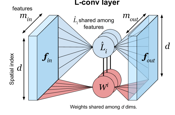
Figure 3: L-conv layer architecture. $L_{i}$ only act on the $d$ flattened spatial dimensions, and $W^{i}$ only act on the $m_{in}$ input features and returns $m_{out}$ output features. For each $i$, L-conv is analogous to a GCN with $d$ nodes and $m_{in}$ features.

To implement L-conv, note that the formula of equation 22 is quite similar to a Graph Convolutional Network (GCN) (Kipf & Welling, 2016). For each $i$, the shared convolutional weights are $\overline{{\epsilon}}^{i}W^{0T}$ and the aggregation function of the GCN, a function of the graph adjacency matrix, is $\hat{L}_{i}$ in L-conv. Thus, L-conv can be implemented as GCN modules for each $\hat{L}_{i}$, plus a residual connection for the ${\bm{f}}W^{0T}$ term.

Figure 3 shows the schematic of the L-conv layer. In a naive implementation, $\hat{L}_{i}$ can be general $d\times d$ matrices. However, being vector fields generated by the Lie algebra, $\hat{L}_{i}$ has a more constrained structure which allows them to be encoded and learned using much fewer parameters than a $d\times d$ matrix. Specifically, encoding the topology of $\mathcal{S}$ as a graph (see SI B.1), the incidence matrix replaces partial derivatives (Schaub et al., 2020) in equation 11 and the $L_{i}$ become weighting of the edges. This weighting is similar to Gauge Equivariant Mesh (GEM) CNN (Cohen et al., 2019a). Indeed, in L-conv the lift ${\bm{x}}_{\mu}=g_{\mu}{\bm{x}}_{0}$ fixes the gauge by mapping neighbors of ${\bm{x}}_{0}$ to neighbors of ${\bm{x}}_{\mu}$. Changing how the discrete $\mathcal{S}$ samples an underlying continuous space will change $g_{\mu}$ and hence the gauge.

Choosing the number of $L_{i}$. Beside the width of $W^{0}$ and $\overline{{\epsilon}}^{i}$, the number $n_{L}$ of $L_{i}$ is a hyperparameter in L-conv. For instance, if $\mathcal{S}$ is a discretization of $n$ dimensional space the symmetry group is likely $G\subset\mathrm{GL}_{n}(\mathbb{R})\ltimes T_{n}$, with $n_{L}\sim O(n^{2})$. Note that $n_{L}$ is independent of the size $d$ of the discretized space (e.g. number of pixels) and generally $n^{2}\ll d$. Choosing $n_{L}$ larger than the true number of $L_{i}$ only results in an over-complete basis and shouldn’t be a problem. We conducted small controlled experiments to verify how multilayer L-conv approximates G-conv (SI C).

Learning symmetries using L-conv.

Rao & Ruderman (1999) introduced a basic version of L-conv and showed that it can learn 1D translation and 2D rotation. We conducted experiments to learn large rotation angle between two images (SI C), shown in Fig. 4. Left shows the architecture for learning the rotation angles between a pair of $7\times 7$ random images ${\bm{f}}$ and $R(\theta){\bm{f}}$ with $\theta\in[0,\pi/3)$. Second left is the learned $L\in SO(2)$ using $3$ recursive layer L-conv. Middle is the $L$ learned using L-conv with fixed small rotation angle $\theta=\pi/10$ (SI C.2) and right is the exact solution $R=(YX^{T})(X^{T}X)^{-1}$. While the middle $L$ is less noisy, it does not capture weights beyond first neighbors of each pixel. (also see SI C for a discussion on symmetry discovery literature.)

L-conv can potentially replace other equivariant layers in a neural network. We conducted limited experiments for this on small image datasets (SI D). L-conv allows one to look for potential symmetries in data which may have been scrambled or harbors hidden symmetries.

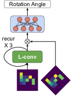
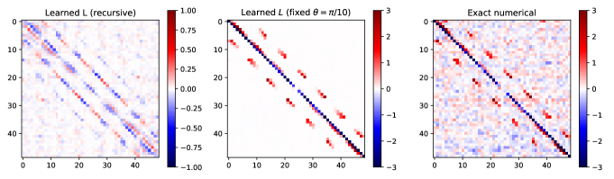
Figure 4: Learning the infinitesimal generator of $SO(2)$ Left shows the architecture for learning rotation angles between pairs of images (SI C.3). Next to it is the $L$ learned using recursive L-conv in this experiment. Middle $L$ is learned using a fixed small rotation angle $\theta=\pi/10$, and right shows $L$ found using the numeric solution from the data.

5 Relation to other architectures

CNN. This is a special case of expressing G-conv as L-conv when the group is continuous 1D translations. The arguments here generalize trivially to higher dimensions. Rao & Ruderman (1999, sec. 4) used the Shannon-Whittaker Interpolation (Whitaker, 1915) to define continuous translation on periodic 1D arrays as ${\bm{f}}^{\prime}_{\rho}=g(z)_{\rho}^{\nu}{\bm{f}}_{\nu}$. Here $g(z)_{\rho}^{\nu}={1\over d}\sum_{p=-d/2}^{d/2}\cos\left({2\pi p\over d}(z+\rho-\nu)\right)$ approximates the shift operator for continuous $z$. These $g(z)$ form a 1D translation group $G$ as $g(w)g(z)=g(w+z)$ with $g(0)^{\nu}_{\rho}=\delta^{\nu}_{\rho}$. For any $z=\mu\in\mathbb{Z}$, $g_{\mu}=g(z=\mu)$ are circulant matrices that shift by $\mu$ as $[g_{\mu}]^{\rho}_{\nu}=\delta^{\rho}_{\nu-\mu}$. Thus, a 1D CNN with kernel size $k$ can be written suing $g_{\mu}$ as

$$F({\bm{f}})_{\nu}^{a} =\sigma\left(\sum_{\mu=0}^{k}{\bm{f}}_{\nu-\mu}^{c}[W^{\mu}]^{a}_{c}+b^{a}\right)=\sigma\left(\sum_{\mu=0}^{k}[g_{\mu}{\bm{f}}]_{\nu}^{c}[W^{\mu}]^{a}_{c}+b^{a}\right)$$ (23)

where $W,b$ are the filter weights and biases. $g_{\mu}$ can be approximated using the Lie algebra and written as multi-layer L-conv as in sec. 3.1. Using $g(0)^{\nu}_{\rho}\approx\delta(\rho-\nu)$, the single Lie algebra basis $[\hat{L}]_{0}=\partial_{z}g(z)|_{z\to 0}$, acts as $\hat{L}f(z)\approx-\partial_{z}f(z)$ (because $\int\partial_{z}\delta(z-\nu)f(z)=-\partial_{\nu}f(\nu)$). Its components are $\hat{L}^{\nu}_{\rho}={L}(\rho-\nu)=\sum_{p}{2\pi p\over d^{2}}\sin\left({2\pi p\over d}(\rho-\nu)\right)$, which are also circulant due to the $(\rho-\nu)$ dependence. Hence, $[\hat{L}{\bm{f}}]_{\rho}=\sum_{\nu}{L}(\rho-\nu){\bm{f}}_{\nu}=[{L}\star{\bm{f}}]_{\nu}$ is a convolution. Rao & Ruderman (1999) already showed that this $\hat{L}$ can reproduce finite discrete shifts $g_{\mu}$ used in CNN. They used a primitive version of L-conv with $g_{\mu}=(I+{\epsilon}\hat{L})^{N}$. Thus, L-conv can approximate 1D CNN. This result generalizes easily to higher dimensions.

Graph Convolutional Network (GCN). Let ${\bm{A}}$ be the adjacency matrix of a graph. In equation 22 if $\hat{L}_{i}=h({\bm{A}})$, such as $\hat{L}_{i}={\bm{D}}^{-1/2}{\bm{A}}{\bm{D}}^{-1/2}$, we obtain a GCN (Kipf & Welling, 2016) (${\bm{D}}_{\mu\nu}=\delta_{\mu\nu}\sum_{\rho}{\bm{A}}_{\mu\rho}$ being the degree matrix). So in the special case where all neighbors of each node $<\mu>$ have the same edge weight, meaning $[\hat{L}_{i}]^{\nu}_{\mu}=[\hat{L}_{i}]^{\rho}_{\mu}$, $\forall\nu,\rho\in<\mu>$, equation 9 is uniformly aggregating over neighbors and L-conv reduces to a GCN. Note that this similarity is not just superficial. In GCN $h({\bm{A}})=\hat{L}$ is in fact a Lie algebra basis. When $\hat{L}=h({\bm{A}})$, the vector field is the flow of isotropic diffusion $d{\bm{f}}/dt=h({\bm{A}}){\bm{f}}$ from each node to its neighbors. This vector field defines one parameter Lie group with elements $g(t)=\exp[h({\bm{A}})t]$. Hence, L-conv for flow groups with a single generator are GCN. These flow groups include Hamiltonian flows and other linear dynamical systems. The main difference between L-conv and GCN is that L-conv can assign a different weight to each neighbor of the same node, similar to GEM-CNN (Cohen et al., 2019a) with a fixed gauge set by $g_{\mu}$. Next, we discuss the mathematical properties of the loss functions for L-conv.

6 Group invariant loss

Loss functions of equivariant networks are rarely discussed. Yet, recent work by Kunin et al. (2020) showed the existence of symmetry directions in the loss landscape. To understand how the symmetry generators in L-conv manifest themselves in the loss landscape, we work out the explicit example of a mean square error (MSE) loss. Because $G$ is the symmetry group, $f$ and $g\cdot f$ should result in the same optimal parameters. Hence, the minima of the loss function need to be group invariant. One way to satisfy this is for the loss itself to be group invariant, which can be constructed by integrating over $G$ (global pooling (Bronstein et al., 2021)). A function $I=\int_{G}dgF(g)$ is $G$-invariant (SI A.3). We can also change the integration to $\int_{\mathcal{S}}d^{n}x$ by change of variable $dg/d{\bm{x}}$ (see SI A.3 for discussion on stabilizers).

MSE loss and Field Theory.

The MSE is given by $I=\sum_{n}\int_{G}dg\|Q[f_{n}](g)\|^{2}$, where $f_{n}$ are data samples and $Q[f]$ is L-conv or another $G$-equivariant function. In supervised learning the input is a pair $f_{n},y_{n}$. $G$ can also act on the labels $y_{n}$. We assme that $y_{n}$ are either also scalar features $y_{n}:\mathcal{S}\to\mathbb{R}^{m_{y}}$ with a group action $g\cdot y_{n}({\bm{x}})=y_{n}(g^{-1}{\bm{x}})$ (e.g. $f_{n}$ and $y_{n}$ are both images), or that $y_{n}$ are categorical. In the latter case $g\cdot y_{n}=y_{n}$ because the only representations of a continuous $G$ on a discrete set are constant. We can concatenate the inputs to $\phi_{n}\equiv[f_{n}|y_{n}]$ with a well-defined $G$ action $g\cdot\phi_{n}=[g\cdot f_{n}|g\cdot y_{n}]$. The collection of combined inputs $\Phi=(\phi_{1},\dots,\phi_{N})^{T}$ is an $(m+m_{y})\times N$ matrix. Using equations 9 and 11, the MSE loss with parameters $W=\{W^{0},\overline{{\epsilon}}\}$ becomes (SI A.3.1)

$$I[\Phi;W] =\int_{G}dg\mathcal{L}[\Phi;W]=\int_{G}dg\left\|W^{0}\left[I+\overline{{\epsilon}}^{i}[\hat{L}_{i}]^{\alpha}\partial_{\alpha}\right]\Phi(g)\right\|^{2}$$ (24)

$$=\int_{\mathcal{S}}{d^{n}x\over\left|\partial x\over\partial g\right|}\left[\Phi^{T}\mathbf{m}_{2}\Phi+\partial_{\alpha}\Phi^{T}\mathbf{h}^{\alpha\beta}\partial_{\beta}\Phi+[\hat{L}_{i}]^{\alpha}\partial_{\alpha}\left(\Phi^{T}\mathbf{v}^{i}\Phi\right)\right]$$ (25)

Equation 25 generalizes the free field theories in physics (Polyakov, 2018). Here $\left|\partial x\over\partial g\right|$ is the determinant of the Jacobian, $W^{i}=W^{0}\overline{{\epsilon}}^{i}$ and

$$\mathbf{m}_{2} =W^{0T}W^{0}, \mathbf{h}^{\alpha\beta}({\bm{x}}) =\overline{{\epsilon}}^{iT}\mathbf{m}_{2}\overline{{\epsilon}}^{j}[\hat{L}_{i}]^{\alpha}[\hat{L}_{j}]^{\beta}, \mathbf{v}^{i} =\mathbf{m}_{2}\overline{{\epsilon}}^{i}.$$ (26)

Note that $\mathbf{h}$ has feature space indices via $[\overline{{\epsilon}}^{iT}\mathbf{m}_{2}\overline{{\epsilon}}^{j}]_{ab}$, with index symmetry $\mathbf{h}^{\alpha\beta}_{ab}=\mathbf{h}^{\beta\alpha}_{ba}$. When $\mathcal{F}=\mathbb{R}$ (i.e. $f$ is a 1D scalar), $\mathbf{h}^{\alpha\beta}$ becomes a a Riemannian metric for $\mathcal{S}$. In general $\mathbf{h}$ combines a 2-tensor $\mathbf{h}_{ab}=\mathbf{h}_{ab}^{\alpha\beta}\partial_{\alpha}\partial_{\beta}\in T\mathcal{S}\otimes T\mathcal{S}$ with an inner product $h^{T}\mathbf{h}^{\alpha\beta}f$ on the feature space $\mathcal{F}$.

In field theory, the motivation is to preserve spatial symmetries for the metric $\mathbf{h}$. In equation 25, $\mathbf{h}$ transforms equivariantly as a 2-tensor $v\cdot\mathbf{h}^{\alpha\beta}=[v^{-1}]^{\alpha}_{\rho}[v^{-1}]^{\beta}_{\gamma}\mathbf{h}^{\rho\gamma}({\bm{x}})$ for $v\in G$ (SI A.3). The last term in equation 25 vanishes for many groups (SI A.3) and it is also absent in physics.

Robustness and Euler-Lagrange Equation. Equivariant neural networks are more robust. To check this, we can quantify how the network would perform for an input $\phi^{\prime}=\phi+\delta\phi$ which adds a small random perturbation $\delta\phi$ to a data point $\phi$. Robustness to such perturbation would mean that, for optimal parameters $W^{*}$ , the loss function would not change, i.e. $I[\phi^{\prime};W^{*}]=I[\phi;W^{*}]$, requiring $I$ to be minimized around real data points $\phi$.

This can be cast as a variational equation $\delta I[\phi;W^{*}]=0$, which yield the familiar Euler-Lagrange (EL) equation (SI A.4). Therefore, for an equivariant network to be robust, i.e. $\delta I[\phi;W^{*}]/\delta\phi=0$, we would require the data points $\phi$ to satisfy the EL equations for optimal parameters $W^{*}$:

$$\mbox{Robustness to random noise}\Longleftrightarrow\mbox{EL: }\quad{\partial\mathcal{L}\over\partial\phi^{b}}-\partial_{\alpha}{\partial\mathcal{L}\over\partial(\partial_{\alpha}\phi^{b})}=0$$ (27)

where the partial derivative terms appear because of the L-conv layer.

Equivariance and Conservation laws. Conserved currents, via Noether’s theorem provide a way to find hidden symmetries (see also Kunin et al. (2020)). The idea is that the equivariance condition equation 2 can be written for the integrand of the loss, $\mathcal{L}[\phi,W]$. If we write the equivariance equation for infinitesimal $v_{\epsilon}$, we obtain a vector field which is divergence free. Since $G$ is the symmetry of the system, transforming an input $\phi\to w\cdot\phi$ by $w\in G$ the integrand should change equivariantly, meaning $\mathcal{L}[w\cdot\phi]=w\cdot\mathcal{L}[\phi]$. When robustness error is minimized as in equation 27, an infinitesimal $w\approx I+\eta^{i}L_{i}$, with $\delta\phi={\epsilon}^{i}\hat{L}_{i}\phi$, results in a conserved current (SI A.4)

$$\mbox{Noether current: }J^{\alpha} ={\partial\mathcal{L}\over\partial(\partial_{\alpha}\phi^{b})}\delta\phi^{b}-{\partial\mathcal{L}\over\partial{\bm{x}}^{\alpha}}\delta{\bm{x}}^{\alpha}, \delta I[\phi;W^{*}]=0\quad\Rightarrow\partial_{\alpha}J^{\alpha} =0$$ (28)

The above equation shows that for equivariant networks with a given symmetry, the deviation in data along the symmetry direction ($\hat{L}_{i}$) yields a divergence free current $J^{\alpha}$, known as Noether current. It also provides an alternative means to discover symmetry generators $L_{i}$ by minimizing $\|\partial_{\alpha}J^{\alpha}\|$. Note that this Noether current is the “stress-energy” tensor, associated with space (or space-time) variations $\delta{\bm{x}}$ (Landau, 2013) (SI A.5). We can potentially design more general equivariant networks leading to other Noether currents.

7 Conclusion and Discussions

We propose the Lie algebra convolutional neural network (L-conv), an infinitesimal version of G-conv. L-conv layers do not require encoding irreps or discretizing the group, and can be combined to approximate any feedforward equivariant networks on compact groups. Additionally, L-conv’s universal and simple structure allows us to discover symmetries from data. It is easy to implement, with a formula similar to GCN. We validated that L-conv can learn the correct Lie algebra basis in a synthetic experiment.

We discover several intriguing connections between L-conv and physics. Our derivation shows that equivariant neural networks based on L-conv lead to Noether’s theorem and conservation laws. Conversely, we can also optimize Noether current to discover symmetries. Furthermore, the current equivariance formulation only pertains to “spatial symmetries” (i.e. $G$ acts on $\mathcal{S}$). In physics, more general “internal symmetries” are quite common (e.g. particle physics). We can potentially design more general equivariant networks with L-conv encoding such symmetries.

Our method also shed lights on scientific machine learning, especially for physical sciences. Physicists generally use simple polynomial forms for the Lagrangian, or the loss function. These “perturbative” Lagrangian lead to divergences in quantum field theory. However, it is believed the true Lagrangian is more complicated. Hence, more expressive L-conv based models can potentially provide more advanced ansatze for solving scientific problems.

Checklist

The checklist follows the references. Please read the checklist guidelines carefully for information on how to answer these questions. For each question, change the default [TODO] to [Yes] , [No] , or [N/A] . You are strongly encouraged to include a justification to your answer, either by referencing the appropriate section of your paper or providing a brief inline description. For example:

• Did you include the license to the code and datasets? [Yes] See Section

• Did you include the license to the code and datasets? [No] The code and the data are proprietary.

• Did you include the license to the code and datasets? [N/A]

Please do not modify the questions and only use the provided macros for your answers. Note that the Checklist section does not count towards the page limit. In your paper, please delete this instructions block and only keep the Checklist section heading above along with the questions/answers below.

1. For all authors…

   1. Do the main claims made in the abstract and introduction accurately reflect the paper’s contributions and scope? [Yes]

   2. Did you describe the limitations of your work? [No]

   3. Did you discuss any potential negative societal impacts of your work? [N/A]

   4. Have you read the ethics review guidelines and ensured that your paper conforms to them? [Yes]

2. If you are including theoretical results…

   1. Did you state the full set of assumptions of all theoretical results? [Yes]

   2. Did you include complete proofs of all theoretical results? [Yes]

3. If you ran experiments…

   1. Did you include the code, data, and instructions needed to reproduce the main experimental results (either in the supplemental material or as a URL)? [Yes]

   2. Did you specify all the training details (e.g., data splits, hyperparameters, how they were chosen)? [Yes]

   3. Did you report error bars (e.g., with respect to the random seed after running experiments multiple times)? [Yes]

   4. Did you include the total amount of compute and the type of resources used (e.g., type of GPUs, internal cluster, or cloud provider)? [Yes]

4. If you are using existing assets (e.g., code, data, models) or curating/releasing new assets…

   1. If your work uses existing assets, did you cite the creators? [Yes]

   2. Did you mention the license of the assets? [N/A]

   3. Did you include any new assets either in the supplemental material or as a URL? [Yes]

   4. Did you discuss whether and how consent was obtained from people whose data you’re using/curating? [N/A]

   5. Did you discuss whether the data you are using/curating contains personally identifiable information or offensive content? [N/A]

5. If you used crowdsourcing or conducted research with human subjects…

   1. Did you include the full text of instructions given to participants and screenshots, if applicable? [N/A]

   2. Did you describe any potential participant risks, with links to Institutional Review Board (IRB) approvals, if applicable? [N/A]

   3. Did you include the estimated hourly wage paid to participants and the total amount spent on participant compensation? [N/A]

Supplementary Information

Appendix A Extended derivations and proofs

Path-ordered Exponential

Every element $g\in G$ can be written as a product $g=\prod_{a}\exp[t_{a}^{i}L_{i}]$ using the matrix exponential (Hall, 2015). This can be done using a path $\gamma$ connecting $I$ to $g$ on the manifold of $G$. Here, $t_{a}$ will be segments of the path $\gamma$ which add up as vectors to connect $I$ to $g$. This surjective map can be written as a “path-ordered” (or time-ordered in physics (Weinberg, 1995)) exponential (POE). In the simplest form, POE can be defined by breaking $u=\prod_{a}\exp[t_{a}^{i}L_{i}]$ down into infinitesimal steps of size $t_{a}=1/N$ with $N\to\infty$. Choosing $\gamma$ to be a differentiable path, we can replace the sum over segments $\sum_{a}t_{a}$ with an integral along the path $\sum_{a}t_{a}=\int_{\gamma}dst(s)ds$, where $t(s)=d\gamma/ds$ is the tangent vector to the path $\gamma$, where $s\in[0,1]$ parametrizes $\gamma$ The POE is then defined as the infinitesimal $t_{a}$ limit of $g=\prod_{a}\exp[t_{a}^{i}L_{i}]$. This can be written as

$$g =P\exp\left[\int_{\gamma}t^{i}(s)L_{i}ds\right]=\lim_{N\to\infty}\prod_{a=1}^{N}\left(I+\delta s{\gamma^{\prime}}^{i}(s_{a})L_{i}\right)$$ (29)

$$=\int_{0}^{s_{1}}ds_{0}{\gamma^{\prime}}^{i}(s_{0})L_{i}\int_{0}^{s_{2}}ds_{1}{\gamma^{\prime}}^{j}(s_{1})L_{j}\dots\int_{0}^{1}ds_{N}{\gamma^{\prime}}^{k}(s_{N})L_{k}$$ (30)

L-conv derivation

Let us consider what happens if the kernel in G-conv equation 3 is localized near identity. Let $\kappa_{I}(u)=c\delta_{\eta}(u)$, with constants $c\in\mathbb{R}^{m^{\prime}}\otimes\mathbb{R}^{m}$ and kernel $\delta_{\eta}(u)\in\mathbb{R}$ which has support only on on an $\eta$ neighborhood of identity, meaning $\delta_{\eta}(I+{\epsilon}^{i}L_{i})\to 0$ if $|{\epsilon}|>\eta$. This allows us to expand G-conv in the Lie algebra of $G$ to linear order. With $v_{\epsilon}=I+{\epsilon}^{i}L_{i}$, we have

$$[\delta_{\eta}\star f](g) =\int_{G}dv\delta_{\eta}(v)f(gv)=\int_{\|{\epsilon}\|<\eta}dv_{\epsilon}\delta_{\eta}(v_{\epsilon})f(gv_{\epsilon})$$ (31)

$$=\int d{\epsilon}\delta_{\eta}(I+{\epsilon}^{i}L_{i})f(g(I+{\epsilon}^{i}L_{i}))$$ (32)

$$=\int d{\epsilon}\delta_{\eta}(I+{\epsilon}^{i}L_{i})f(g+{\epsilon}^{i}gL_{i})$$ (33)

$$=\int d{\epsilon}\delta_{\eta}(I+{\epsilon}^{i}L_{i})\left[f(g)+{\epsilon}^{i}gL_{i}\cdot{d\over dg}f(g)+O({\epsilon}^{2})\right]$$ (34)

$$=\int d{\epsilon}\delta_{\eta}(I+{\epsilon}^{i}L_{i})\left[I+{\epsilon}^{i}gL_{i}\cdot{d\over dg}\right]f(g)+O(\eta^{2})$$ (35)

$$=W^{0}\left[I+\overline{{\epsilon}}^{i}gL_{i}\cdot{d\over dg}\right]f(g)+O(\eta^{2})$$ (36)

where $d{\epsilon}$ is the integration measure on the Lie algebra induced by the Haar measure $dv$ on $G$. The $O(\eta^{2})$ term arises from integrating the $O({\epsilon}^{2})$ terms. To see this, note that for an order $p$ function $\phi(\epsilon)$, for $|\epsilon|<\eta$, $|\phi(\epsilon)|<\eta^{p}C$ (for some constant $C$). Substituting this bound into the integral over the kernel $\delta_{\eta}$ we get

$$\left|\int d\epsilon\delta_{\eta}(I+\epsilon^{i}L_{i})\phi(\epsilon)\right|\leq\int\left|d\epsilon\delta_{\eta}(I+\epsilon^{i}L_{i})\phi(\epsilon)\right|$$ (37)

$$<\int\left|d\epsilon\delta_{\eta}(I+\epsilon^{i}L_{i})\eta^{p}C\right|\leq\eta^{p}C\int\left|d\epsilon\delta_{\eta}(I+\epsilon^{i}L_{i})\right|\leq\eta^{p}C$$ (38)

In matrix representations, $gL_{i}\cdot{df\over dg}=[gL_{i}]_{\alpha}^{\beta}{df\over dg_{\alpha}^{\beta}}=\mathrm{Tr}\left[[gL_{i}]^{T}{df\over dg}\right]$. Note that in $g(I+{\epsilon}^{i}L_{i}){\bm{x}}_{0}$, the $gL_{i}{\bm{x}}_{0}=\hat{L}_{i}{(g)}{\bm{x}}$ come from the pushforward $\hat{L}_{i}{(g)}=gL_{i}g^{-1}\in T_{g}G$. Here

$$W^{0} =c\int d{\epsilon}\delta_{\eta}(I+{\epsilon}^{i}L_{i})\in\mathbb{R}^{m^{\prime}}\otimes\mathbb{R}^{m}, \overline{{\epsilon}}^{i} =\frac{\int d{\epsilon}\delta_{\eta}(I+{\epsilon}^{i}L_{i}){\epsilon}^{i}}{\int d{\epsilon}\delta_{\eta}(I+{\epsilon}^{i}L_{i})}\in\mathbb{R}^{m}\otimes\mathbb{R}^{m}$$ (39)

with $\|\overline{{\epsilon}}\|<\eta$. When $\delta_{\eta}$ is normalized, meaning $\int_{G}\delta_{\eta}(g)dg=1$, we have $W^{0}=c$ and

$$\overline{{\epsilon}}^{i} =\int d{\epsilon}\delta_{\eta}(I+{\epsilon}^{i}L_{i}){\epsilon}^{i}$$

Note that with $f(g)\in\mathbb{R}^{m}$, each ${\epsilon}^{i}\in\mathbb{R}^{m}\otimes\mathbb{R}^{m}$ is a matrix. With indices, $f(gv_{\epsilon})$ is given by

$$[f(gv_{\epsilon})]^{a} =\sum_{b}f^{b}(g(\delta^{a}_{b}+[{\epsilon}^{i}]^{a}_{b}L_{i}))$$ (40)

Similarly, the integration measure $d{\epsilon}$, which is induced by the Haar measure $dv_{\epsilon}\equiv d\mu(v_{\epsilon})$, is a product $\int d{\epsilon}=\int|J|\prod d[{\epsilon}^{i}]^{a}_{b}$, with $J=\partial v_{\epsilon}/\partial{\epsilon}$ being the Jacobian.

Equation 36 is the core of the architecture we are proposing, the Lie algebra convolution or L-conv.

L-conv Layer In general, we define Lie algebra convolution (L-conv) as follows

$$Q[f](g) =W^{0}\left[I+\overline{{\epsilon}}^{i}gL_{i}\cdot{d\over dg}\right]f(g)$$ (41)

$$=[W^{0}]_{b}f^{a}\left(g\left(\delta^{b}_{a}+[\overline{{\epsilon}}^{i}]_{a}^{b}L_{i}\right)\right)+O(\overline{{\epsilon}}^{2})$$ (42)

Extended equivariance for L-conv

From equation 42 we see that $W^{0}$ acts on the output feature indices. Notice that the equivariance of L-conv is due to the way $gv_{\epsilon}=g(I+\overline{{\epsilon}}^{i}L_{i})$ appears in the argument, since for $u\in G$

$$u\cdot Q[f](g)=W^{0}f(u^{-1}gv_{\epsilon})=W^{0}[u\cdot f](gv_{\epsilon})$$ (43)

Because of this, replacing $W^{0}$ with a general neural network which acts on the feature indices separately will not affect equivariance. For instance, if we pass L-conv through a neural network to obtain a generalized L-conv $Q_{\sigma}$, we have

$$Q_{\sigma}[f](g) =\sigma(Wf(gv_{\epsilon})+b)$$ (44)

$$u\cdot Q_{\sigma}[f](g) =Q_{\sigma}[f](u^{-1}g)=\sigma(Wf(u^{-1}gv_{\epsilon})+b)$$ (45)

$$=\sigma(W[u\cdot f](gv_{\epsilon})+b)=Q_{\sigma}[u\cdot f](g)$$ (46)

Thus, L-conv can be followed by any nonlinear neural network as long as it only acts on the feature indices (i.e. $a$ in $f^{a}(g)$) and not on the spatial indices $g$ in $f(g)$.

A.1 Approximating G-conv using L-conv

Lemma 1 (Approximating the kernel). Let the kernel $\kappa:G\to\mathcal{F}^{\prime}\otimes\mathcal{F}$ with $\int_{G}\|\kappa(g)\|^{2}dg<\infty$ be continuously differentiable with $\|d\kappa(g)/dg\|^{2}<\xi^{2}$, and with compact support over $G_{0}\subset G$. Let $\kappa_{k}(g)=c_{k}\delta_{\eta}(u_{k}^{-1}g)$ be a set of kernels with support on an $\eta$ neighborhood of $u_{k}\in G$. Then, $\exists c_{k}\in\mathcal{F}^{\prime}\otimes\mathcal{F},u_{k}\in G$ such that $\tilde{\kappa}$ approximates $\kappa$, meaning $\int_{G}\|\kappa(g)-\tilde{\kappa}(g)\|^{2}dg<\zeta^{2}$ for arbitrary small $\zeta\in\mathbb{R}_{+}$.

Proof: The intuition is similar to the universal approximation theorem for neural networks (Hornik et al., 1989; Cybenko, 1989), only generalized to a group manifold instead of $\mathbb{R}$. Let $B_{0}$ be the set of $v_{\epsilon}=I+{\epsilon}^{i}L_{i}\in\mathfrak{g}$, with $\|{\epsilon}\|^{2}<\eta^{2}$. Choose a finite set of $u_{k}\in G$ such that the neighborhoods $B_{k}=u_{k}B_{0}\subset G$, and such that $\bigcup_{k}B_{k}=G_{0}$. We can show that, for small enough $\eta$, the kernel does not change more than $\xi$ over each $B_{k}$, allowing us to replace it with a constant localized kernel $\kappa_{k}$ with support only on $B_{k}$. To see this, consider $g\in B_{k}$ and $v_{\epsilon}=I+{\epsilon}^{i}L_{i}\in\mathfrak{g}$, such that $v_{\epsilon}g\in B_{k}$. Let $\gamma$ be a path connecting $g$ to $v_{\epsilon}g$, via $u(s)=(I+s{\epsilon}^{i}L_{i})g$, with $s\in[0,1]$. Using the triangle inequality we have

$$\|\kappa(g)-\kappa(v_{\epsilon}g)\|^{2} =\left\|\int_{\gamma}ds{d\kappa(u(s))\over ds}\right\|^{2}\leq\int_{\gamma}ds\left\|{d\kappa(u(s))\over ds}\right\|^{2}$$ (47)

$$<\int_{0}^{1}ds\left\|dg\over ds\right\|^{2}\xi^{2}=\|{\epsilon}\|^{2}\xi^{2}$$ (48)

where $\|{\epsilon}\|^{2}\leq\eta^{2}$ because $v_{\epsilon}g\in B_{k}$. This means that if we replace $\kappa(g)$ with $\kappa(u_{k})$ for any $u_{k}\in B_{k}$, our error in approximating $\kappa$ over $B_{k}$ is less than $\eta^{2}\xi^{2}$. Setting $\kappa_{k}(g)=\kappa(u_{k})\delta_{\eta}(u_{k}^{-1}g)$ with the localized kernels $\delta_{\eta}(g)$ being any continuously differentiable distribution such that $\int_{B_{k}}dg\delta_{\eta}(u_{k}^{-1}g)=1$ on all $B_{k}$, we get

$$\int_{G}dg\|\kappa(g)-\tilde{\kappa}(g)\|^{2}=\sum_{k}\int_{B_{k}}dg\|\kappa(g)-\kappa_{k}(g)\|^{2}<\sum_{k}|B_{k}|\eta^{2}\xi^{2}=|G_{0}|\eta^{2}\xi^{2}$$ (49)

where $|G_{0}|$ is the volume of the support of $\kappa$ $\square$

Thus, we can approximate a large class of kernels as $\kappa(g)\approx\sum_{k}\kappa_{k}(g)$ where the local kernels $\kappa_{k}(g)=c_{k}\delta_{\eta}(u_{k}^{-1}g)$ have support only on an $\eta$ neighborhood of $u_{k}\in G$. Here $c_{k}\in\mathbb{R}^{m^{\prime}}\otimes\mathbb{R}^{m}$ are constants and $\delta_{\eta}(u)$ is as in equation 9. Using this, G-conv equation 3 becomes

$$[\kappa\star f](g) =\sum_{k}c_{k}\int dv\delta_{\eta}(u_{k}^{-1}v)f(gv)=\sum_{k}c_{k}[\delta_{\eta}\star f](gu_{k}).$$ (50)

The kernels $\kappa_{k}$ are localized around $u_{k}$, whereas in L-conv the kernel is around identity. We can compose L-conv layers to move $\kappa_{k}$ from $u_{k}$ to identity.

Lemma 2 (Moving kernels to identity). The local kernel $\kappa_{k}$ can be moved near identity using a multilayer L-conv.

Proof: In equation 50, write $u_{k}=v_{\epsilon}u^{\prime}_{k}$, with $v_{\epsilon}=I+{\epsilon}^{i}L_{i}\in\mathfrak{g}$. We have

$$\delta_{\eta}(u_{k}^{-1}v) =\left.\left[I+{\epsilon}^{i}gL_{i}\cdot{d\over dg}\right]\delta_{\eta}(g)\right|_{g\to{u^{\prime}}_{k}^{-1}v}+O({\epsilon}^{2})\approx Q_{\epsilon}[\delta_{\eta}]({u^{\prime}}_{k}^{-1}v)$$ (51)

where $Q_{{\epsilon}}=I-{\epsilon}^{i}\hat{L}_{i}$ is an L-conv layer with $W^{0}=I$. This means that applying one L-conv layer with the parameters above moves the localized kernel along $v_{\epsilon}$ on $G$. Iterating this further, write $u_{k}$ as the product of a set of small group elements $u_{k}=\prod_{a=1}^{p}v_{a}$, with $v_{a}=I+{\epsilon}_{a}^{i}L_{i}\in\mathfrak{g}$. Defining L-conv layers $Q_{a}=I-{\epsilon}_{a}^{i}\hat{L}_{i}$, we can write

$$\kappa_{k}(g) \approx c_{k}Q_{p}\circ\cdots\circ Q_{1}\circ\delta_{\eta}(g)$$ (52)

meaning $\kappa_{k}$ localized around $u_{k}$ can be written as a $p$ layer L-conv acting on a kernel $\delta_{\eta}(g)$, localized around the identity of the group. With $\|{\epsilon}_{a}\|<\eta$, the error in $u_{k}$ is $O(\eta^{p+1})$. $\square$

Thus, we conclude that any G-conv equation 3 can be approximated by multilayer L-conv. We can take this result even further, following the main theorem in Kondor & Trivedi (2018), and show that any feedforward equivariant neural network can be approximated using multilayer L-conv with nonlinearities.

Equivariance of nonlinearity Pointwise nonlinearities give equivariant maps between scalar feature maps. To see this, let $\sigma:\mathbb{R}\to\mathbb{R}$. We extend $\sigma:{\mathcal{F}}\to{\mathcal{F}}$ by applying $\sigma$ component-wise. Let $f:\mathcal{S}\to\mathcal{F}$ be a scalar feature map (i.e., $g\cdot f({\bm{x}})=f(g^{-1}{\bm{x}})$). Then

$$g\cdot(\sigma\circ(f))({\bm{x}})=\sigma\circ(f)(g^{-1}{\bm{x}})=\sigma\circ(g\cdot f)({\bm{x}}).$$

Since the composition of equivariant maps is equivariant, given equivariant linear mapping $Q:\mathcal{F}^{\mathcal{S}}\to\mathcal{F}^{\prime{\mathcal{S}}}$ (i.e. $g\cdot Q[f]=Q[g\cdot f]$), the layer $f\mapsto\sigma\circ Q[f]$ is equivariant. Hence we have the corollary:

Corollary 2.

Assume $G$ is compact and acts on ${\mathcal{S}}$ transitively. Then any equivariant feedforward neural network (FNN) can be approximated using multilayer L-conv with point-wise nonlinearities. Without the compactness and transitivity hypothesis, multilayer L-conv with pointwise non-linearities can approximate multilayer G-conv with pointwise non-linearities.

Proof: A FNN is defined as $\sigma_{p}\circ F_{p}[\cdots[\sigma_{1}\circ F_{1}[f]]({\bm{x}})$ where $F_{k}$ are linear and $\sigma_{k}$ are point-wise nonlinearities. By Theorem 1 of Kondor & Trivedi (2018), any linear equivariant layer is a G-conv, which by Theorem LABEL:thm:Gconv2Lconv can be approximated by multilayer L-conv. Therefore, multilayer L-conv with nonlinearity can approximate any equivariant FNN. $\square$

Finally, note that to our knowledge it is not known whether every equivariant function can be approximated by equivariant FNN for a Lie group $G$. Hence, the corollary above is not a universal approximation theorem for equivariant scalar functions in terms of L-conv. However, it does show that multilayer $L$-conv is equally expressive as other equivariant networks.

Since many datasets such as images deal with discretized spaces, we first need to derive how L-conv acts on such data, discussed next.

A.2 Example of continuous L-conv

The $gL_{i}\cdot df/dg$ in equation 9 can be written in terms of partial derivatives $\partial_{\alpha}f({\bm{x}})=\partial f/\partial{\bm{x}}^{\alpha}$. In general, using ${\bm{x}}^{\rho}=g^{\rho}_{\sigma}{\bm{x}}_{0}^{\sigma}$, we have

$${df(g{\bm{x}}_{0})\over dg^{\alpha}_{\beta}} ={d(g^{\rho}_{\sigma}{\bm{x}}_{0}^{\sigma})\over dg^{\alpha}_{\beta}}\partial_{\rho}f({\bm{x}})={\bm{x}}_{0}^{\beta}\partial_{\alpha}f({\bm{x}})$$ (53)

$$gL_{i}\cdot{df\over dg} =[gL_{i}]^{\alpha}_{\beta}{\bm{x}}_{0}^{\beta}\partial_{\alpha}f({\bm{x}})=[gL_{i}{\bm{x}}_{0}]\cdot\nabla f({\bm{x}})=\hat{L}_{i}f({\bm{x}})$$ (54)

Hence, for each $L_{i}$, the pushforward $gL_{i}$ generates a flow on $\mathcal{S}$ through the vector field $\hat{L}_{i}\equiv gL_{i}\cdot d/dg=[gL_{i}{\bm{x}}_{0}]^{\alpha}\partial_{\alpha}$ (Fig. 1). Being a vector field $\hat{L}_{i}\in T\mathcal{S}$ (i.e. 1-tensor), $\hat{L}_{i}$ is basis independent, meaning for $v\in G$, $\hat{L}_{i}(v{\bm{x}})=\hat{L}_{i}$. Its components transform as $[\hat{L}_{i}(v{\bm{x}})]^{\alpha}=[vgL_{i}{\bm{x}}_{0}]^{\alpha}=v^{\alpha}_{\beta}\hat{L}_{i}({\bm{x}})^{\beta}$, while the partial transforms as $\partial/\partial[v{\bm{x}}]^{\alpha}=[v^{-1}]^{\gamma}_{\alpha}\partial_{\gamma}$. Using this relation and Taylor expanding equation 15, we obtain a second form for the group action on L-conv. For $w\in G$, with ${\bm{y}}=w^{-1}{\bm{x}}$ we have

$$Q[f](w^{-1}g{\bm{x}}_{0}) =W^{0}\left[I+\overline{{\epsilon}}^{i}[\hat{L}_{i}]^{\alpha}[w^{-1}]^{\beta}_{\alpha}{\partial\over\partial{\bm{y}}^{\beta}}\right]f({\bm{y}})\big{|}_{{\bm{y}}\to w^{-1}{\bm{x}}}$$ (55)

1D Translation: Let $G=T_{1}=(\mathbb{R},+)$. A matrix representation for $G$ is found by encoding $x$ as a a 2D vector $(x,1)$. The lift is given by ${\bm{x}}_{0}=(0,1)$ as the origin and $g=\begin{pmatrix}1&x\\ 0&1\end{pmatrix}$. The Lie algebra basis is $L=\begin{pmatrix}0&1\\ 0&0\end{pmatrix}$. It is easy to check that $gg^{\prime}{\bm{x}}_{0}=(x+x^{\prime},1)$. We also find $gL=L$, meaning $L$ looks the same in all $T_{g}G$. Close to identity $I=0$, $v_{\epsilon}=I+{\epsilon}L={\epsilon}$. We have $gv_{\epsilon}{\bm{x}}_{0}=(g+{\epsilon}gL)x_{0}=(x+{\epsilon},1)$. Thus, $f(g(I+{\epsilon}L){\bm{x}}_{0})\approx f({\bm{x}})+{\epsilon}df({\bm{x}})/d{\bm{x}}$. This readily generalizes to $n$D translations $T_{n}$ (SI A.2.2), yielding $f({\bm{x}})+{\epsilon}^{\alpha}\partial_{\alpha}f({\bm{x}})$.

2D Rotation:

Let $G=SO(2)$. The space which $SO(2)$ can lift is not the full $\mathbb{R}^{2}$, but a circle of fixed radius $r=\sqrt{x^{2}+y^{2}}$. Hence we choose $\mathcal{S}=S^{1}$ embedded in $\mathbb{R}^{2}$, with $x=r\cos\theta$ and $y=r\sin\theta$. For the lift, we use the standard 2D representation. We have ${\bm{x}}_{0}=(r,0)$ and (see SI A.2.1)

$$L =\begin{pmatrix}0&-1\\ 1&0\end{pmatrix}, g =\exp[\theta L]={1\over r}\begin{pmatrix}x&-y\\ y&x\end{pmatrix}, gL\cdot{df\over dg} =\left(x\partial_{y}-y\partial_{x}\right)f.$$ (56)

Physicists will recognize $\hat{L}\equiv\left(x\partial_{y}-y\partial_{x}\right)=\partial_{\theta}$ as the angular momentum operator in quantum mechanics and field theories, which generates rotations around the $z$ axis.

Rotation and scaling

Let $G=SO(2)\times\mathbb{R}^{+}$, where the $\mathbb{R}^{+}=[0,\infty)$ is scaling. The infinitesimal generator for scaling is identity $L_{2}=I$. This group is also Abelian, meaning $[L_{2},L]=0$ ($L\in so(2)$ equation 56). $\mathbb{R}^{2}/{0}$ can be lifted to $G$ by choosing ${\bm{x}}_{0}=(1,0)$ in polar coordinates and ${\bm{x}}=g{\bm{x}}_{0}=rL_{2}\exp[\theta L]{\bm{x}}_{0}$. We again have $gL\cdot df/dg=\partial_{\theta}f$. We also have $gL_{2}=g$, so $gL_{2}{\bm{x}}_{0}=(x,y)$ and from equation 54, $gL_{2}\cdot df/dg=(x\partial_{x}+y\partial_{y})f=r\partial_{r}f$, which is the scaling operation.

A.2.1 Rotation $SO(2)$

With ${\bm{x}}_{0}=(r,0)$

$$g =\begin{pmatrix}\cos\theta&-\sin\theta\\ \sin\theta&\cos\theta\end{pmatrix},={1\over r}\begin{pmatrix}x&-y\\ y&x\end{pmatrix}, L =\begin{pmatrix}0&-1\\ 1&0\end{pmatrix} gL ={1\over r}\begin{pmatrix}-y&-x\\ x&-y\end{pmatrix}$$ (57)

$$gL{\bm{x}}_{0} =\begin{pmatrix}-y\\ x\end{pmatrix}=\begin{pmatrix}-\sin\theta\\ \cos\theta\end{pmatrix}$$ (58)

To calculate $df/dg$ we note that even after the lift, the function $f$ was defined on $\mathcal{S}$. So we must include the ${\bm{x}}_{0}$ in $f(g{\bm{x}}_{0})$. Using equation 11, we have

$${df(g{\bm{x}}_{0})\over dg} ={1\over r}{\bm{x}}_{0}^{T}\begin{pmatrix}\partial_{x}f&-\partial_{y}f\\ \partial_{y}f&\partial_{x}f\end{pmatrix}=\begin{pmatrix}\partial_{x}f&-\partial_{y}f\\ 0&0\end{pmatrix}$$ (59)

$$gL\cdot{df\over dg} =\mathrm{Tr}\begin{pmatrix}x\partial_{y}f-y\partial_{x}f&x\partial_{x}f+y\partial_{y}f\\ 0&0\end{pmatrix}=\left(x\partial_{y}f-y\partial_{x}f\right)$$ (60)

A.2.2 Translations $T_{n}$

Generalizing the $T_{1}$ case, we add a dummy dimension $0$ and ${\bm{x}}_{0}=(1,0,\dots,0)$. The generators are $[L_{i}]_{\mu}^{\nu}=\delta_{i\mu}\delta_{0}^{\nu}$ and $g=I+x^{i}L_{i}$. Again, $gL_{i}=L_{i}+x^{j}L_{j}L_{i}=L_{i}$ as $L_{j}L_{i}=0$ for all $i,j$. Hence, $[\hat{L}_{i}]^{\alpha}=[gL_{i}{\bm{x}}_{0}]^{\alpha}=\delta^{\alpha}_{i}$.

A.3 Group invariant loss

Because $G$ is the symmetry group, $f$ and $g\cdot f$ should result in the same optimal parameters. Hence, the minima of the loss function need to be group invariant. One way to satisfy this is for the loss itself to be group invariant, which can be constructed by integrating over $G$ (global pooling (Bronstein et al., 2021)). A function $I=\int_{G}dgF(g)$ is $G$-invariant as for $w\in G$

$$w\cdot I =\int_{G}w\cdot F(g)dg=\int F(w^{-1}g)dg=\int_{G}F(g^{\prime})d(wg^{\prime})=\int_{G}F(g^{\prime})dg^{\prime}$$ (61)

where we used the invariance of the Haar measure $d(wg^{\prime})=dg^{\prime}$. We can change the integration to $\int_{\mathcal{S}}d^{n}x$ by change of variable $dg/d{\bm{x}}$. Since we need $\mathcal{S}$ to be lifted to $G$, the lift$:\mathcal{S}\to G$ is injective, the a map $G\to\mathcal{S}$ need not be. $\mathcal{S}$ is homeomorphic to $G/H$, where $H\subset G$ is the stabilizer of the origin, i.e. $h{\bm{x}}_{0}={\bm{x}}_{0},\forall h\in H$. Since $F(g{\bm{x}}_{0})=F(gh{\bm{x}}_{0})$, we have

$$I =\int_{G}F(g)dg=\int_{H}dh\int_{G/H}dg^{\prime}F(g^{\prime})=V_{H}\int_{G/H}dg^{\prime}F(g^{\prime})$$ (62)

Since $G/H\sim\mathcal{S}$, the volume forms $dg^{\prime}=V_{H}d^{n}x$ can be matched for some parametrization.

A.3.1 MSE Loss

The MSE is given by $I=\sum_{n}\int_{G}dg\|Q[f_{n}](g)\|^{2}$, where $f_{n}$ are data samples and $Q[f]$ is L-conv or another $G$-equivariant function. In supervised learning the input is a pair $f_{n},y_{n}$. $G$ can also act on the labels $y_{n}$. We assme that $y_{n}$ are either also scalar features $y_{n}:\mathcal{S}\to\mathbb{R}^{m_{y}}$ with a group action $g\cdot y_{n}({\bm{x}})=y_{n}(g^{-1}{\bm{x}})$ (e.g. $f_{n}$ and $y_{n}$ are both images), or that $y_{n}$ are categorical. In the latter case $g\cdot y_{n}=y_{n}$ because the only representations of a continuous $G$ on a discrete set are constant. We can concatenate the inputs to $\phi_{n}\equiv[f_{n}|y_{n}]$ with a well-defined $G$ action $g\cdot\phi_{n}=[g\cdot f_{n}|g\cdot y_{n}]$. The collection of combined inputs $\Phi=(\phi_{1},\dots,\phi_{N})^{T}$ is an $(m+m_{y})\times N$ matrix. Using equations 9 and 11, the MSE loss with parameters $W=\{W^{0},\overline{{\epsilon}}\}$ becomes

$$I[\Phi;W] =\int_{G}dg\mathcal{L}[\Phi;W]=\int_{G}dg\left\|W^{0}\left[I+\overline{{\epsilon}}^{i}[\hat{L}_{i}]^{\alpha}\partial_{\alpha}\right]\Phi(g)\right\|^{2}$$ (63)

$$=2\int_{G}dg\left[\|W^{0}\Phi\|^{2}+\left\|W^{i}[\hat{L}_{i}]^{\alpha}\partial_{\alpha}\Phi\right\|^{2}+2\Phi^{T}W^{0T}W^{i}[\hat{L}_{i}]^{\alpha}\partial_{\alpha}\Phi\right]$$ (64)

$$=\int_{\mathcal{S}}{d^{n}x\over\left|\partial x\over\partial g\right|}\left[\Phi^{T}\mathbf{m}_{2}\Phi+\partial_{\alpha}\Phi^{T}\mathbf{h}^{\alpha\beta}\partial_{\beta}\Phi+[\hat{L}_{i}]^{\alpha}\partial_{\alpha}\left(\Phi^{T}\mathbf{v}^{i}\Phi\right)\right]$$ (65)

where $\left|\partial x\over\partial g\right|$ is the determinant of the Jacobian, $W^{i}=W^{0}\overline{{\epsilon}}^{i}$ and

$$\mathbf{m}_{2} =W^{0T}W^{0}, \mathbf{h}^{\alpha\beta}({\bm{x}}) =\overline{{\epsilon}}^{iT}\mathbf{m}_{2}\overline{{\epsilon}}^{j}[\hat{L}_{i}]^{\alpha}[\hat{L}_{j}]^{\beta}, \mathbf{v}^{i} =\mathbf{m}_{2}\overline{{\epsilon}}^{i}.$$ (66)

From equation 64 to 65 we used the fact that $W^{0}$ and $W^{i}$ do not depend on ${\bm{x}}$ (or $g$) to write

$$2\Phi^{T}W^{0T}W^{i}[\hat{L}_{i}]^{\alpha}\partial_{\alpha}\Phi =[\hat{L}_{i}]^{\alpha}\partial_{\alpha}\left(\Phi^{T}W^{0T}W^{i}\Phi\right)=[\hat{L}_{i}]^{\alpha}\partial_{\alpha}\left(\Phi^{T}\mathbf{m}_{2}\overline{{\epsilon}}^{i}\Phi\right)$$ (67)

Note that $\mathbf{h}$ has feature space indices via $[\overline{{\epsilon}}^{iT}\mathbf{m}_{2}\overline{{\epsilon}}^{j}]_{ab}$, with index symmetry $\mathbf{h}^{\alpha\beta}_{ab}=\mathbf{h}^{\beta\alpha}_{ba}$. When $\mathcal{F}=\mathbb{R}$ (i.e. $f$ is a 1D scalar), $\mathbf{h}^{\alpha\beta}$ becomes a a Riemannian metric for $\mathcal{S}$. In general $\mathbf{h}$ combines a 2-tensor $\mathbf{h}_{ab}=\mathbf{h}_{ab}^{\alpha\beta}\partial_{\alpha}\partial_{\beta}\in T\mathcal{S}\otimes T\mathcal{S}$ with an inner product $h^{T}\mathbf{h}^{\alpha\beta}f$ on the feature space $\mathcal{F}$. Hence $\mathbf{h}\in T\mathcal{S}\otimes T\mathcal{S}\otimes\mathcal{F}^{*}\otimes\mathcal{F}^{*}$ is a $(2,2)$-tensor, with $\mathcal{F}^{*}$ being the dual space of $\mathcal{F}$.

Loss invariant metric transformation

The metric $\mathbf{h}$ transforms equivariantly as a 2-tensor. As discussed under equation 11, $[\hat{L}_{i}(v{\bm{x}})]^{\alpha}=v^{\alpha}_{\beta}\hat{L}_{i}({\bm{x}})^{\beta}$ and

$$v\cdot\mathbf{h}^{\alpha\beta} =\mathbf{h}^{\alpha\beta}(v^{-1}{\bm{x}})=[v^{-1}]^{\alpha}_{\rho}[v^{-1}]^{\beta}_{\gamma}\mathbf{h}^{\rho\gamma}({\bm{x}}), (v \in G).$$ (68)

Note that $v\cdot\mathbf{m}_{2}=\mathbf{m}_{2}$ since $f_{n}$ and $y_{n}$ are scalars. For example, let $G=SO(2)$ and $R(\xi)\in SO(2)$ be rotation by angle $\xi$. Since there is only one $L_{i}=L$, the metric factorizes to

$$\mathbf{h}^{\alpha\beta}_{ab}=[\overline{{\epsilon}}^{T}\mathbf{m}_{2}\overline{{\epsilon}}]_{ab}\otimes[\hat{L}\hat{L}^{T}]^{\alpha\beta}$$ (69)

To find $R(\xi)\cdot\mathbf{h}$ we only need to calculate $R(\xi)^{-1}\hat{L}$. With $g=R(\theta)$, we have $\hat{L}({\bm{x}})=R(\theta)L{\bm{x}}_{0}=(-y,x)=r(-\sin\theta,\cos\theta)$ from equation 58. Therefore, $R(\xi)^{-1}\hat{L}=R(\theta-\xi)=\hat{L}(R(\xi^{-1}{\bm{x}})$. Using equation 26 in equation 68, the transformed metric becomes

$$R(\xi)\cdot\mathbf{h}^{\alpha\beta}(R(\theta){\bm{x}}_{0})=\overline{{\epsilon}}^{T}\mathbf{m}_{2}\overline{{\epsilon}}\otimes[R(-\xi)\hat{L}]^{\alpha}[R(-\xi)\hat{L}]^{\beta}=\mathbf{h}^{\alpha\beta}(R(\theta-\xi){\bm{x}}_{0}),$$ (70)

A.3.2 Third term as a boundary term

Since terms in equation 25 are scalars, they can be evaluated in any basis. If $\mathcal{S}$ can be lifted to multiple Lie groups, either group can be used to evaluate equation 25. For example $\mathbb{R}^{n}/0$ can be lifted to both $T_{n}$ and $SO(n)\times\mathbb{R}_{+}$. For the translation group $G=T_{n}$ we have $gL_{i}=L_{i}$ and $[\hat{L}_{i}]^{\alpha}=\delta^{\alpha}_{i}$ (SI A.2.2) and $|\partial g/\partial x|=1$ and $dg=d^{n}x$. Thus, the last term in equation 25 simplifies to a complete divergence $\int d^{n}x\partial_{i}(\Phi^{T}\mathbf{v}^{i}\Phi)$. Using the generalized Stoke’s theorem $\int_{\mathcal{S}}dw=\int_{\partial\mathcal{S}}w$, the last term in equation 25 becomes a boundary term. When $\mathcal{S}$ is non-compact, the last term is $I_{\partial}=\int_{\partial\mathcal{S}}d\Sigma_{i}\Phi^{T}\mathbf{v}^{i}\Phi$, where $d\Sigma_{i}$ is the normal times the volume form of the $(n-1)$D boundary $\partial\mathcal{S}$ and is in the radial direction (e.g. for $\mathcal{S}=\mathbb{R}^{n}$ the boundary is a hyper-sphere $\partial\mathcal{S}=S^{n-1}$). Generally we expect the features $\phi_{n}$ to be concentrated in a finite region of the space and that they go to zero as $r\to\infty$ (if they don’t the loss term $\Phi^{T}\mathrm{m}_{2}\Phi$ will diverge). Thus, the last term in equation 25 generally becomes a vanishing boundary term and does not matter.

A.3.3 MSE Loss for translation group $T_{n}$

We have $gL_{i}=L_{i}$ and $[\hat{L}_{i}]^{\alpha}=\delta^{\alpha}_{i}$ (SI A.2.2), the last term in equation 25 becomes a complete divergence $I_{\partial}=\int d^{n}x\partial_{i}(\Phi^{T}\mathbf{v}^{i}\Phi)$. Using the generalized Stoke’s theorem $\int_{\mathcal{S}}dw=\int_{\partial\mathcal{S}}w$, when $\mathcal{S}$ is non-compact, $I_{\partial}=\int_{\partial\mathcal{S}}d\Sigma_{i}\Phi^{T}\mathbf{v}^{i}\Phi$. Here $d\Sigma_{i}$ is the normal times the volume form of the $(n-1)$D boundary $\partial\mathcal{S}$ (e.g. for $\mathcal{S}=\mathbb{R}^{n}$ the boundary is a hyper-sphere $\partial\mathcal{S}=S^{n-1}$). Generally we expect the features $\phi_{n}$ to be concentrated in a finite region of the space and that they go to zero as $r\to\infty$ (if they don’t the loss term $\Phi^{T}\mathrm{m}_{2}\Phi$ will diverge). Thus, the last term in equation 25 generally becomes a vanishing boundary term and does not matter.

Next, the second term in equation 25 can be worked out as

$$\hat{L}_{i}^{\alpha}\partial_{\alpha}\phi^{T}\overline{{\epsilon}}^{iT}\mathbf{m}_{2}\overline{{\epsilon}}^{j}\hat{L}_{j}^{\beta}\partial_{\beta}\phi =\partial_{j}\phi^{T}\overline{{\epsilon}}^{iT}\mathbf{m}_{2}\overline{{\epsilon}}^{j}\partial_{i}\phi=\partial_{j}\phi^{T}\mathbf{h}^{ji}\partial_{i}\phi$$ (71)

where $\mathbf{h}^{ji}=\overline{{\epsilon}}^{iT}\mathbf{m}_{2}\overline{{\epsilon}}^{j}$ is a general, space-independent metric compatible with translation symmetry. When the weights $[W^{i}]^{a}_{b}\sim\mathcal{N}(0,1)$ are random Gaussian, we have $W^{jT}W^{i}\approx m^{2}\delta^{ij}$ and we recover the Euclidean metric. With the lst term vanishing, the loss function equation 25 has a striking resemblance to a Lagrangian used in physics, as we discuss next.

A.3.4 Boundary term with spherical symmetry

When $\mathcal{S}\sim\mathbb{R}^{n}$ and $G=T_{n}$, the third term becomes a boundary term. But we can also have $G=SO(n)\times\mathbb{R}_{+}$ (spherial symmetry and scaling). The boundary $\partial\mathcal{S}\sim S^{n-1}$, which has an $SO(n)$ symmetry. The normal $d\Sigma({\bm{x}})$ is a vector pointing in the radial direction and $g$ is the lift for ${\bm{x}}$. Since $g\in SO(n)$, we have

$$d\Sigma_{\beta}[gL_{\alpha}{\bm{x}}_{0}]^{\beta} =d\Sigma^{T}gL_{\alpha}{\bm{x}}_{0}=[g^{T}d\Sigma]^{T}L_{\alpha}{\bm{x}}_{0}$$ (72)

Since $g\in SO(n)$, $g^{T}=g^{-1}$ and $g^{T}d\Sigma(g{\bm{x}}_{0})=d\Sigma({\bm{x}}_{0})=V_{n-1}{\bm{x}}_{0}$, meaning the normal vector is rotated back toward ${\bm{x}}_{0}$. Here $V_{n-1}$ is the volume of the boundary $S^{n-1}$. Hence we have

$$d\Sigma^{T}gL_{i}{\bm{x}}_{0}={\bm{x}}_{0}^{T}L_{i}{\bm{x}}_{0}=0$$ (73)

for all generators $L_{i}\in so(n)$ because $L_{i}=-L_{i}^{T}$ and hence diagonal entries like ${\bm{x}}_{0}^{T}L_{i}{\bm{x}}_{0}$ are zero. Only the scaling generator $L_{0}=I$ we have ${\bm{x}}_{0}^{T}L_{0}{\bm{x}}_{0}=1$. This means that the last term in equation 25 can be nonzero at the boundary only if $\Phi\mathbf{v}^{i}\Phi$ is in the radial direction, meaning $\overline{{\epsilon}}^{0}=0$, and $\Phi$ does not vanish at the boundary. However, a non-vanishing $\Phi$ at the boundary results in diverging loss unless the mass matrix $\mathbf{m}_{2}$ has eigenvalues equal to zero. This is what happens relativistic theories where light rays can have nonzero $\Phi$ at infinity because they are massless.

A.4 Robustness to random noise

Equivariant neural networks are hoped to be more robust than others. One way to check this is to see how the network would perform for an input $\phi^{\prime}=\phi+\delta\phi$ which adds a small perturbation $\delta\phi$ to a real data point $\phi$. Robustness to such perturbation would mean that, for optimal parameters $W^{*}$, the loss function would not change, i.e. $I[\phi^{\prime};W^{*}]=I[\phi;W^{*}]$. This can be cast as a variational equation, requiring $I$ to be minimized around real data points $\phi$. Writing $I[\phi;W]=\int d^{n}x\mathcal{L}[\phi;W]$, we have

$$\delta I[\phi;W^{*}] =\int_{\mathcal{S}}d^{n}x\left[{\partial\mathcal{L}\over\partial\phi^{a}}\delta\phi^{a}+{\partial\mathcal{L}\over\partial(\partial_{\alpha}\phi^{a})}\partial_{\alpha}(\delta\phi^{a})\right]$$ (74)

Doing a partial integration on the second term, we get

$$\delta I[\phi;W^{*}] =\int_{\mathcal{S}}d^{n}x\left[{\partial\mathcal{L}\over\partial\phi^{b}}-\partial_{\alpha}{\partial\mathcal{L}\over\partial(\partial_{\alpha}\phi^{b})}\right]\delta\phi^{b}+\int_{\mathcal{S}}d^{n}x\partial_{\alpha}\left[{\partial\mathcal{L}\over\partial(\partial_{\alpha}\phi^{b})}\delta\phi^{b}\right]$$ (75)

$$=\int_{\mathcal{S}}d^{n}x\left[{\partial\mathcal{L}\over\partial\phi^{b}}-\partial_{\alpha}{\partial\mathcal{L}\over\partial(\partial_{\alpha}\phi^{b})}\right]\delta\phi^{b}+\int_{\partial\mathcal{S}}d^{n-1}\Sigma_{\alpha}\left[{\partial\mathcal{L}\over\partial(\partial_{\alpha}\phi^{b})}\delta\phi^{b}\right]$$ (76)

If we want equivariant networks to be robust, then both terms in equation 76 need to be zero. We show that the first term is the classic Euler-Lagrange (EL) equation, and the second term is related to conservation laws.

We use the Stoke’s theorem to change the second term to a boundary integral. Since features $\phi$ have finite support, $\phi({\bm{x}})\to 0$ as $|{\bm{x}}|\to\infty$, and the boundary term vanishes. The first term in equation 76 is the classic Euler-Lagrange (EL) equation. Thus, requiring robustness, i.e. $\delta I[\phi;W^{*}]/\delta\phi=0$ means for optimal parameters $W^{*}$, the data $\phi$ satisfies the EL equations

$$\mbox{Robustness to random noise}\Longleftrightarrow\mbox{EL: }\quad{\partial\mathcal{L}\over\partial\phi^{b}}-\partial_{\alpha}{\partial\mathcal{L}\over\partial(\partial_{\alpha}\phi^{b})}=0$$ (77)

Applying this to the MSE loss equation 25, equation 77 becomes

$$\mathbf{m}_{2}\phi-\partial_{\alpha}\left(|J|\mathbf{h}^{\alpha\beta}\partial_{\beta}\phi\right)-\partial_{\alpha}\left(|J|\mathbf{v}^{i}[\hat{L}_{i}]^{\alpha}\right)\phi=0$$ (78)

where $|J|=|\partial g/\partial x|$ is the determinant of the Jacobian. For the translation group, equation 78 becomes a Helmholtz equation

$$\mathbf{h}^{ij}\partial_{i}\partial_{j}\phi=\overline{{\epsilon}}^{i}\mathbf{m}_{2}\overline{{\epsilon}}^{j}\partial_{i}\partial_{j}\phi=\mathbf{m}_{2}\phi$$ (79)

where $\mathbf{h}^{ij}\partial_{i}\partial_{j}=\nabla^{2}$ is the Laplace-Beltrami operator with $\mathbf{h}$ as the metric.

A.5 Conservation laws

The equivariance condition equation 2 can be written for the integrand of the loss $\mathcal{L}[\phi,W]$. Since $G$ is the symmetry of the system, transforming an input $\phi\to w\cdot\phi$ by $w\in G$ the integrand changes equivariantly as $\mathcal{L}[w\cdot\phi]=w\cdot\mathcal{L}[\phi]$. Now, let $w$ be an infinitesimal $w\approx I+\eta^{i}L_{i}$. The action $w\cdot\phi$ can be written as a Taylor expansion, similar to the one in L-conv, yielding

$$w\cdot\phi({\bm{x}}) =\phi(w^{-1}{\bm{x}})=\phi((I-\eta^{i}L_{i}){\bm{x}})=\phi({\bm{x}})-\eta^{i}[L_{i}{\bm{x}}]^{\alpha}\partial_{\alpha}\phi({\bm{x}})$$ (80)

$$=\phi({\bm{x}})+\delta{\bm{x}}^{\alpha}\partial_{\alpha}\phi({\bm{x}})=\phi({\bm{x}})+\delta\phi({\bm{x}})$$ (81)

with $\delta{\bm{x}}^{\alpha}=-\eta^{i}[L_{i}{\bm{x}}]^{\alpha}$ and $\delta\phi=\delta{\bm{x}}^{\alpha}\partial_{\alpha}\phi$. Similarly, we have $w\cdot\mathcal{L}=\mathcal{L}+\delta{\bm{x}}^{\alpha}\partial_{\alpha}\mathcal{L}$. Next, we can use the chain rule to calculate $\mathcal{L}[w\cdot\phi]$.

$$\mathcal{L}[w\cdot\phi] =\mathcal{L}[\phi({\bm{x}})+\delta\phi({\bm{x}})]=\mathcal{L}[\phi]+{\partial\mathcal{L}\over\partial\phi^{b}}\delta\phi^{b}+{\partial\mathcal{L}\over\partial(\partial_{\alpha}\phi^{b})}\delta\partial_{\alpha}\phi^{b}$$ (82)

$$=\mathcal{L}[\phi]+\left[{\partial\mathcal{L}\over\partial\phi^{b}}-\partial_{\alpha}{\partial\mathcal{L}\over\partial(\partial_{\alpha}\phi^{b})}\right]\delta\phi^{b}+\partial_{\alpha}\left({\partial\mathcal{L}\over\partial(\partial_{\alpha}\phi^{b})}\delta\phi^{b}\right)$$ (83)

where we used the fact that $\delta{\bm{x}}=\eta^{i}L_{i}{\bm{x}}$ can vary independently from ${\bm{x}}$ (because of $\eta^{i}$), and so $\delta\partial_{\alpha}\phi^{b}=\partial_{\alpha}\delta\phi^{b}$. The same way, $\delta{\bm{x}}^{\alpha}\partial_{\alpha}\mathcal{L}=\partial_{\alpha}(\delta{\bm{x}}^{\alpha}\mathcal{L})$. Now, if $\phi$ are the real data and the parameters in $\mathcal{L}$ minimize generalization error, then $\mathcal{L}$ satisfies equation 78. This means that the first term in equation 83 vanishes. Setting the second term equal to $w\cdot\mathcal{L}$ we get

$$\mathcal{L}[w\cdot\phi]-w\cdot\mathcal{L}[\phi] =\partial_{\alpha}\left[{\partial\mathcal{L}\over\partial(\partial_{\alpha}\phi^{b})}\delta\phi^{b}-\delta{\bm{x}}^{\alpha}\mathcal{L}\right]=0$$ (84)

Thus, the terms in the brackets are divergence free. These terms are called a Noether conserved current $J^{\alpha}$. In summary

$$\mbox{Noether current: }J^{\alpha} ={\partial\mathcal{L}\over\partial(\partial_{\alpha}\phi^{b})}\delta\phi^{b}-{\partial\mathcal{L}\over\partial{\bm{x}}^{\alpha}}\delta{\bm{x}}^{\alpha}, \delta I[\phi;W^{*}]=0\quad\Rightarrow\partial_{\alpha}J^{\alpha} =0$$ (85)

$J$ captures the change of the Lagrangian $\mathcal{L}$ along symmetry direction $\hat{L}_{i}$. Plugging $\delta\phi=\delta{\bm{x}}^{\alpha}\partial_{\alpha}\phi$from equation 81 we find

$$\partial_{\alpha}\left[{\partial\mathcal{L}\over\partial(\partial_{\alpha}\phi^{b})}\delta\phi^{b}-\delta{\bm{x}}^{\alpha}\mathcal{L}\right]=\delta{\bm{x}}^{\beta}\partial_{\alpha}\left[{\partial\mathcal{L}\over\partial(\partial_{\alpha}\phi^{b})}\partial_{\beta}\phi^{b}-\delta^{\alpha}_{\beta}\mathcal{L}\right]=\delta{\bm{x}}^{\beta}\partial_{\alpha}T^{\alpha}_{\beta}.$$ (86)

$T^{\alpha}_{\beta}$ is known as the stress-energy tensor in physics (Landau, 2013). It is the Noether current associated with space (or space-time) variations $\delta{\bm{x}}$. It appears here because $G$ acts on the space, as opposed to acting on feature dimensions. For the MSE loss we have

$$T^{\alpha}_{\beta}\equiv {\partial\mathcal{L}\over\partial(\partial_{\alpha}\phi^{b})}\partial_{\beta}\phi^{b}-\delta^{\alpha}_{\beta}\mathcal{L}=\partial_{\rho}\phi^{T}\left(\delta^{\lambda}_{\beta}\mathbf{h}^{\alpha\rho}-\delta^{\alpha}_{\beta}\mathbf{h}^{\rho\lambda}\right)\partial_{\lambda}\phi-\phi^{T}\mathbf{m}_{2}\phi$$ (87)

It would be interesting to see if the conserved currents can be used in practice as an alternative way for identifying or discovering symmetries.

Appendix B Tensor notation details

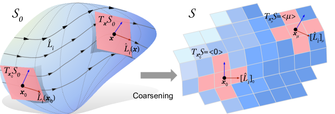
Figure 5: Manifold vs. discretized Space While real systems can have a continuous manifold $\mathcal{S}_{0}$ as their base space, often the data collected from is a discrete array $\mathcal{S}$. The discretization (coarsening) will induce some of the topology of $\mathcal{S}_{0}$ on $\mathcal{S}$ as a graph. Graph neighborhoods $<\mu>$ on the discrete $\mathcal{S}$ represent tangent spaces $T_{{\bm{x}}_{\mu}}\mathcal{S}$ and approximate $T_{\bm{x}}\mathcal{S}_{0}$. The lift takes ${\bm{x}}\in\mathcal{S}_{0}$ to $g\in G$, and maps the tangent spaces $T_{\bm{x}}\mathcal{S}_{0}\to T_{g}G$. Each Lie algebra basis $L_{i}\in\mathfrak{g}=T_{I}G$ generates a vector field on the tangent bundle $TG$ via the pushforward as $L^{(g)}=gL_{i}g^{-1}$. Due to the lift, each $L_{i}$ also generates a vector field $\hat{L}_{i}^{\alpha}({\bm{x}})\partial_{\alpha}=[gL_{i}{\bm{x}}_{0}]^{\alpha}\partial_{\alpha}$, with ${\bm{x}}=g{\bm{x}}_{0}$. Analogously, on $\mathcal{S}$ we get a vector field $[\hat{L}_{i}]_{\mu}=g_{\mu}L_{i}{\bm{x}}_{0}$ on $T\mathcal{S}$, with ${\bm{x}}_{\mu}=g_{\mu}{\bm{x}}_{0}$. Note that depicting $\mathcal{S}$ and $\mathcal{S}_{0}$ as 2D is only for convenience. They may have any dimensions.

If the dataset being analyzed is in the form of $f({\bm{x}})$ for some sample of points ${\bm{x}}$, together with derivatives $\nabla f({\bm{x}})$, we can use the L-conv formulation above. However, in many datasets, such as images, $f({\bm{x}})$ is given as a finite dimensional array or tensor, with ${\bm{x}}$ taking values over a grid. Even though the space $\mathcal{S}$ is now discrete, the group which acts on it can still be continuous (e.g. image rotations). Let $\mathcal{S}=\{{\bm{x}}_{0},\dots\bm{x}_{d-1}\}$ contain $d$ points. Each ${\bm{x}}_{\mu}$ represents a coordinate in higher dimensional grid. For instance, on a $10\times 10$ image, ${\bm{x}}_{0}$ is $(x,y)=(0,0)$ point and ${\bm{x}}_{99}$ is $(x,y)=(9,9)$.

Feature maps

To define features $f({\bm{x}}_{\mu})\in\mathbb{R}^{m}$ for ${\bm{x}}_{\mu}\in\mathcal{S}$, we embed ${\bm{x}}_{\mu}\in\mathbb{R}^{d}$ and encode them as the canonical basis (one-hot) vectors with components $[{\bm{x}}_{\mu}]^{\nu}=\delta_{\mu}^{\nu}$ (Kronecker delta), e.g. ${\bm{x}}_{0}=(1,0,\dots,0)$. The feature space becomes $\mathcal{F}=\mathbb{R}^{d}\otimes\mathbb{R}^{m}$, meaning feature maps ${\bm{f}}\in\mathcal{F}$ are $d\times m$ tensors, with $f({\bm{x}}_{\mu})={\bm{x}}_{\mu}^{T}{\bm{f}}={\bm{f}}_{\mu}$.

Group action

Any subgroup $G\subseteq\mathrm{GL}_{d}(\mathbb{R})$ of the general linear group (invertible $d\times d$ matrices) acts on $\mathbb{R}^{d}$ and $\mathcal{F}$. Since ${\bm{x}}_{\mu}\in\mathbb{R}^{d}$, $g\in G$ also naturally act on ${\bm{x}}_{\mu}$. The resulting ${\bm{y}}=g{\bm{x}}_{\mu}$ is a linear combination ${\bm{y}}=c^{\nu}{\bm{x}}_{\nu}$ of elements of the discrete $\mathcal{S}$, not a single element. The action of $G$ on ${\bm{f}}$ and ${\bm{x}}$, can be defined in multiple equivalent ways. We define $f(g\cdot{\bm{x}}_{\mu})={\bm{x}}_{\mu}^{T}g^{T}{\bm{f}},\forall g\in G$. For $w\in G$ we have

$$w\cdot f({\bm{x}}_{\mu}) =f(w^{-1}\cdot{\bm{x}}_{\mu})={\bm{x}}_{\mu}^{T}w^{-1T}{\bm{f}}=[w^{-1}{\bm{x}}]^{T}{\bm{f}}$$ (88)

Dropping the position ${\bm{x}}_{\mu}$, the transformed features are matrix product $w\cdot{\bm{f}}=w^{-1T}{\bm{f}}$.

G-conv and L-conv in tensor notation

Writing G-conv equation 3 in the tensor notation we have

$$[\kappa\star f](g{\bm{x}}_{0})=\int_{G}\kappa(v)f(gv{\bm{x}}_{0})dv={\bm{x}}_{0}^{T}\int_{G}v^{T}g^{T}{\bm{f}}\kappa^{T}(v)dv\equiv{\bm{x}}_{0}^{T}[{\bm{f}}\star\kappa](g)$$ (89)

where we moved $\kappa^{T}(v)\in\mathbb{R}^{m}\otimes\mathbb{R}^{m^{\prime}}$ to the right of ${\bm{f}}$ because it acts as a matrix on the output index of ${\bm{f}}$. The equivariance of equation 89 is readily checked with $w\in G$

$$w\cdot[{\bm{f}}\star\kappa](g) =[{\bm{f}}\star\kappa](w^{-1}g)=\int_{G}v^{T}g^{T}w^{-1T}{\bm{f}}\kappa^{T}(v)dv=[(w\cdot{\bm{f}})\star\kappa](g)$$ (90)

where we used $[w^{-1}g]^{T}{\bm{f}}=g^{T}w^{-1T}{\bm{f}}$. Similarly, we can rewrite L-conv equation 9 in the tensor notation. Defining $v_{\epsilon}=I+\overline{{\epsilon}}^{i}L_{i}$

$$Q[{\bm{f}}](g) =W^{0}f\left(g\left(I+\overline{{\epsilon}}^{i}L_{i}\right)\right)={\bm{x}}_{0}^{T}\left(I+\overline{{\epsilon}}^{i}L_{i}\right)^{T}g^{T}{\bm{f}}W^{0T}$$ (91)

$$=\left({\bm{x}}_{0}+\overline{{\epsilon}}^{i}[gL_{i}{\bm{x}}_{0}]\right)^{T}{\bm{f}}W^{0T}.$$ (92)

Here, $\hat{L}_{i}=gL_{i}{\bm{x}}_{0}$ is eactly the tensor analogue of pushforward vector field $\hat{L}_{i}$ in equation 11. We will make this analogy more precise below. The equivariance of L-conv in tensor notation is again evident from the $g^{T}{\bm{f}}$, resulting in

$$Q[w\cdot{\bm{f}}](g) ={\bm{x}}_{0}^{T}v_{\epsilon}^{T}g^{T}w^{-1T}{\bm{f}}W^{0T}=Q[{\bm{f}}](w^{-1}g)=w\cdot Q[{\bm{f}}](g)$$ (93)

Next, we will discuss how to implement equation 92 in practice and how to learn symmetries with L-conv. We will also discuss the relation between L-conv and other neural architectures.

B.1 Constraints from topology on tensor L-conv

To implement equation 92 we need to specify the lift and the form of $L_{i}$. We will now discuss the mathematical details leading to and easy to implement form of equation 92.

Topology

Although he discrete space $\mathcal{S}$ is a set of points, in many cases it has a topology. For instance, $\mathcal{S}$ can be a discretization of a manifold $\mathcal{S}_{0}$, or vertices on a lattice or a general graph. We encode this topology in an undirected graph (i.e. 1-simplex) with vertex set $\mathcal{S}$ edge set $\mathcal{E}$. Instead of the commonly used graph adjacency matrix ${\bm{A}}$, we will use the incidence matrix ${\bm{B}}:\mathcal{S}\times\mathcal{E}\to\{0,1,-1\}$. ${\bm{B}}^{\mu}_{\alpha}=1$ or $-1$ if edge $\alpha$ starts or ends at node $\mu$, respectively, and ${\bm{B}}^{\mu}_{\alpha}=0$ otherwise (undirected graphs have pairs of incoming and outgoing edges ). Similar to the continuous case we will denote the topological space $(\mathcal{S},\mathcal{E},{\bm{B}})$ simply by $\mathcal{S}$.

Figure 5 summarizes some of the aspects of the discretization as well as analogies between $\mathcal{S}_{0}$ and $\mathcal{S}$. Technically, the group $G_{0}$ acting on $\mathcal{S}_{0}$ and $G$ acting on $\mathcal{S}$ are different. But we can find a group $G$ which closely approximates $G_{0}$ (see SI B.2). For instance, Rao & Ruderman (1999) used Shannon-Whittaker interpolation theorem (Whitaker, 1915) to define continuous 1D translation and 2D rotation groups on discrete data. We return to this when expressing CNN as L-conv in 5.

Neighborhoods as discrete tangent bundle

${\bm{B}}$ is useful for extending differential geometry to graphs (Schaub et al., 2020). Define the neighborhood $<\mu>=\left\{\alpha\in\mathcal{E}\big{|}{\bm{B}}_{\alpha}^{\mu}=-1\right\}$ of ${\bm{x}}_{\mu}$ as the set of outgoing edges. $<\mu>$ can be identified with $T_{{\bm{x}}_{\mu}}\mathcal{S}$ as for $\alpha\in<\mu>$, ${\bm{B}}_{\alpha}{\bm{f}}={\bm{f}}_{\mu}-{\bm{f}}_{\nu}\sim\partial_{\alpha}{\bm{f}}$, where $\mu$ and $\nu$ are the endpoints of edge $\alpha$. This relation becomes exact when $\mathcal{S}$ is an $n$D square lattice with infinitesimal lattice spacing. The set of all neighborhoods is ${\bm{B}}$ itself and encodes the approximate tangent bundle $T\mathcal{S}$. For some operator $C:\mathcal{S}\otimes\mathcal{F}\to\mathcal{F}$ acting on ${\bm{f}}$ we will say $C\in<\mu>$ if its action remains within vertices connected to $\mu$, meaning

$$C\in<\mu>:\qquad C{\bm{f}}=\sum_{\alpha\in<\mu>}\tilde{C}^{\alpha}{\bm{B}}_{\alpha}^{\nu}{\bm{f}}_{\nu}$$ (94)

Lift and group action

Lie algebra elements $L_{i}$ by definition take the origin ${\bm{x}}_{0}$ to points close to it. Thus, for small enough $\eta$, $(I+\eta L_{i}){\bm{x}}_{0}\in<0>$ and so $[L_{i}{\bm{x}}_{0}]^{T}{\bm{f}}=[\hat{L}_{i}]_{0}^{\rho}{\bm{f}}_{\rho}=\sum_{\alpha\in<0>}[\hat{\ell}_{i}]_{0}^{\alpha}{\bm{B}}^{\rho}_{\alpha}{\bm{f}}_{\rho}$. The coefficients $[\hat{\ell}_{i}]_{0}^{\alpha}\in\mathbb{R}$ are in fact the discrete version of $\hat{L}_{i}$ components from equation 11. For the pushforward $gL_{i}g^{-1}$, we define the lift via ${\bm{x}}_{\mu}=g_{\mu}{\bm{x}}_{0}$. We require the $G$-action to preserve the topology of $\mathcal{S}$, meaning points which are close remain close after the $G$-action. As a result, $<\mu>$ can be reached by pushing forward elements in $<0>$. Thus, for each $i$, $\exists\eta\ll 1$ such that $g_{\mu}(I+\eta L_{i}){\bm{x}}_{0}\in<\mu>$, meaning for a set of coefficients $[\hat{L}_{i}]_{\mu}^{\nu}\in\mathbb{R}$ we have

$$[g_{\mu}(I+\eta L_{i}){\bm{x}}_{0}]^{T}{\bm{f}} ={\bm{f}}_{\mu}+\eta\sum_{\alpha\in<\mu>}[\hat{\ell}_{i}]_{\mu}^{\alpha}{\bm{B}}_{\alpha}^{\nu}{\bm{f}}_{\nu}$$ (95)

where ${\bm{f}}_{\mu}={\bm{x}}_{\mu}^{T}{\bm{f}}$. Acting with $[g_{\mu}L_{i}{\bm{x}}_{0}]^{T}{\bm{x}}_{\nu}$ and inserting $I=\sum_{\rho}{\bm{x}}_{\rho}{\bm{x}}_{\rho}^{T}$ we have

$$[\hat{L}_{i}]_{\mu}^{\nu} =[\hat{\ell}_{i}]_{\mu}^{\alpha}{\bm{B}}_{\alpha}^{\nu}=[g_{\mu}L_{i}{\bm{x}}_{0}]^{\nu}=\sum_{\rho}[g_{\mu}{\bm{x}}_{\rho}{\bm{x}}^{T}_{\rho}L_{i}{\bm{x}}_{0}]^{T}{\bm{x}}_{\nu}$$ (96)

$$=\sum_{\rho\in<0>}[L_{i}]_{0}^{\rho}[{\bm{x}}_{\nu}^{T}g_{\mu}{\bm{x}}_{\rho}]^{T}=[L_{i}]_{0}^{\rho}[g_{\mu}]^{\nu}_{\rho}=[\hat{\ell}_{i}]_{0}^{\alpha}{\bm{B}}_{\alpha}^{\rho}[g_{\mu}]^{\nu}_{\rho}$$ (97)

This $\hat{L}_{i}\equiv\hat{\ell}_{i}^{\alpha}{\bm{B}}_{\alpha}$ is the discrete $\mathcal{S}$ version of the vector field $\hat{L}_{i}({\bm{x}})=[gL_{i}{\bm{x}}_{0}]^{\alpha}\partial_{\alpha}$ in equation 11.

B.2 Approximating a symmetry and discretization error

Discretization error

While systems such as crystalline solids are discrete in nature, many other datasets such as images result from discretization of continuous data. The discretization (or “coarsening” (Bronstein et al., 2021)) will modify the groups that can act on the space. For example, first rotating a shape by $SO(2)$ then taking a picture is different from first taking a picture then rotating the picture (i.e. group action and discretization do not commute). Nevertheless, in most cases in physics and machine learning the symmetry group $G_{0}$ of the space before discretization has a small Lie algebra dimension $n$, (e.g. $SO(3),SE(3),SO(3,1)$ etc). Usually the resolution of the discretization is $d\gg n$. In this case, there always exist some $G\subseteq\mathrm{GL}_{d}(\mathbb{R})$ which approximates $G_{0}$ reasonably well. The approximation means $\forall g_{0}\in G_{0},\exists g\in G$ such that the error $\mathcal{L}_{G}=\|g_{0}\cdot f({\bm{x}}_{\mu})-{\bm{x}}_{\mu}^{T}g{\bm{f}}\|^{2}<\eta^{2}$ where $\eta$ depends on the resolution of the discretization. Minimizing the error $\mathcal{L}_{G}$ can be the process of identifying the $G$ which best approximates $G_{0}$. We will denote this approximate similarity as $G\simeq G_{0}$. For example, Rao & Ruderman (1999) used the Shannon-Whittaker Interpolation theorem (Whitaker, 1915) to translate discrete 1D signals (features) by arbitrary, continuous amounts. In this case the transformed features are ${\bm{f}}^{\prime}_{\mu}=g(z)_{\mu}^{\nu}{\bm{f}}_{\nu}$, where $g(z)_{\mu}^{\nu}={1\over d}\sum_{p=-d/2}^{d/2}\cos\left({2\pi p\over d}(z+\mu-\nu)\right)$ approximates the shift operator for continuous $z$. The $g(z)$ form a group because $g(w)g(z)=g(w+z)$, which is a representation for periodic 1D shifts. Rao & Ruderman (1999) also use a 2D version of the interpolation theorem to approximate $SO(2)$. In practice, we can assume the true symmetry to be $G$, as we only have access to the discretized data and can’t measure $G_{0}$ directly.

B.3 Comparison with other symmetry discovery methods

Meta-learning Symmetries by Reparameterization

Recently Zhou et al. (2020) also introduced an architecture which can learn equivariances from data. We would like to highlight the differences between their approach and ours, specifically Proposition 1 in Zhou et al. (2020). Assuming a discrete group $G=\{g_{1},\dots,g_{n}\}$, they decompose the weights $W\in\mathbb{R}^{s\times s}$ of a fully-connected layer, acting on ${\bm{x}}\in\mathbb{R}^{s}$ as $\mathrm{vec}(W)=U^{G}v$ where $U^{G}\in\mathbb{R}^{s\times s}$ are the “symmetry matrices” and $v\in\mathbb{R}^{s}$ are the “filter weights”. Then they use meta-learning to learn $U^{G}$ and during the main training keep $U^{G}$ fixed and only learn $v$. We may compare MSR to our approach by setting $d=s$. First, note that although the dimensionality of $U\in\mathbb{R}^{nd\times d}$ seems similar to our $L\in\mathbb{R}^{n\times d\times d}$, the $L_{i}$ are $n$ matrices of shape $d\times d$, whereas $U$ has shape $(nd)\times d$ with many more parameters than $L$. Also, the weights of L-conv $W\in\mathbb{R}^{n\times m_{l}\times m_{l-1}}$, with $m_{l}$ being the number of channels, are generally much fewer than MSR filters $v\in\mathbb{R}^{d}$. Finally, the way in which $Uv$ acts on data is different from L-conv, as the dimensions reveal. The prohibitively high dimensionality of $U$ requires MSR to adopt a sparse-coding scheme, mainly Kronecker decomposition. Though not necessary, we too choose to use a sparse format for $L_{i}$, finding that very low-rank $L_{i}$ often perform best. A Kronecker decomposition may bias the structure of $U^{G}$ as it introduces a block structure into it.

Augerino

In a concurrent work, (Benton et al., 2020) propose Augerino, a method to learn equivariance with neural networks, but restricted to a subgroup of the augmentation transformations. Augerino learns which subset of the augmentations improved the prediction. This is done by writing The data augmentation is written as $g_{\epsilon}=\exp\left(\sum_{i}{\epsilon}_{i}\theta_{i}L_{i}\right)$ (equation (9) in Benton et al. (2020)), with randomly sampled ${\epsilon}_{i}\in[-1,1]$. $\theta_{i}$ are trainable weights which determine which $L_{i}$ helped with the learning task. Furthermore, Their Lie algebra is fixed to affine transformations in 2D (translations, rotations, scaling and shearing). Our approach is more general. We learn the $L_{i}$ directly without restricting to known symmetries. Additionally, we do not use the exponential map or matrix logarithm, hence, our method is easy to implement. Lastly, Augerino uses sampling to effectively cover the space of group transformations. Since we work with the Lie algebra rather the group itself, we do not require sampling.

Appendix C Experiments

We conduct a set of experiments to see how well L-conv can extract infinitesimal generators.

Nonlinear activation

As noted in Weiler et al. (2018a), an arbitrary nonlinear activation $\sigma$ may not keep the architecture equivariant under $G$. However, as we showed in SI A (Extended equivariance for L-conv), the feature dimensions can pass through any nonlinear neural network without affecting the equivariance of L-conv. This means that the weights of the nonlinear layer should act only on $\mathcal{F}$ and not $\mathcal{S}$.

Implementation

The basic way to implement L-conv is as multiple parallel GCN units with aggregation function $f(A)$ being (propagation rule) being $\hat{L}_{i}$. We do not use Deep Graph Library (DGL) or other libraries, as we want to make $\hat{L}_{i}$ learnable for discovering symmetries. A more detailed way to implement L-conv is to encode $\hat{L}_{i}$ in the form of equation 97 to ensure that there is an underlying shared generator $\hat{\ell}_{i}$ for all $\mu$ which is pushed forward using $g_{\mu}$, shared for all $i$. To implement L-conv this way, we need the lift $g_{\mu}$ and the edge weights $w_{i}^{\alpha}=[\hat{\ell}_{i}]_{0}^{\alpha}$. With known symmetries, the learnable parameters are $W^{0}$ and $\overline{{\epsilon}}^{i}$. When the topology and hence ${\bm{B}}$ is known, we can encode it into the geometry and only learn the edge weights $[\hat{\ell}_{i}]^{\alpha}_{\mu}$, similar to edge features in message passing neural networks (MPNN) (Gilmer et al., 2017). In general each $\hat{\ell}_{i}$ has $|\mathcal{E}|$ (i.e. number of edges) components. We can further reduce these using equation 97, where instead of $n$ matrices $\hat{\ell}_{i}$, we learn one $g_{\mu}$ shared for all, and a small set of elements $[\hat{\ell}_{i}]_{0}^{\alpha}$. This is easiest when the graph is a regular lattice and each vertex has the same number of neighbors. When the topology of the underlying space is not known (e.g. point cloud or scrambled coordinates), we can learn $\hat{L}_{i}$ as $d\times d$ matrices. We do this for the scrambled image tests, where we encode $\hat{L}_{i}$ as low-rank matrices.

Symmetry Discovery Literature

In addition to simplifying the construction of equivariant architectures, our method can also learn the symmetry generators from data. Learning symmetries from data has been studied before, but mostly in restricted settings. Examples include commutative Lie groups as in Cohen & Welling (2014), 2D rotations and translations in Rao & Ruderman (1999), Sohl-Dickstein et al. (2010) or permutations (Anselmi et al., 2019). Zhou et al. (2020) uses meta-learning to automatically learn symmetries in the data. Yet their weight-sharing scheme and the encoding of the symmetry generators is very different from ours. (Benton et al., 2020) propose Augerino, a method to learn equivariance with neural networks, but restricted to a subgroup of the augmentation transformations. Their Lie algebra is fixed to affine transformations in 2D (translations, rotations, scaling and shearing). Our approach is more general. We learn the $L_{i}$ directly without restricting to known symmetries. Additionally, we do not use the exponential map or matrix logarithm, hence, our method is easy to implement. Lastly, Augerino uses sampling to effectively cover the space of group transformations. Since we work with the Lie algebra rather the group itself, we do not require sampling.

C.1 Approximating 1D CNN

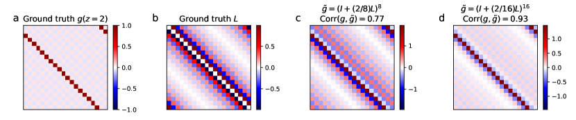
Figure 6: 1D Translation: Using the Shannon-Whittaker Interpolation (SWI) one can generate continuous shifts on discrete data. These include integer shifts (a, ground truth). (SWI) also yields an infinitesimal generator $L$ for shifts (b). This $L$ can be used to approximate finite shifts using $\tilde{g}_{n}(z)=(I+z/nL)^{n}$, with $n\to\infty$ yielding $\exp[zL]$. (c) and (d) show the approximation of a shift by two pixels using $n=8$ and $n=16$.

As discussed in the text, Rao & Ruderman (1999, sec. 4) used the Shannon-Whittaker Interpolation (SWI) (Whitaker, 1915) to define continuous translation on periodic 1D arrays as ${\bm{f}}^{\prime}_{\rho}=g(z)_{\rho}^{\nu}{\bm{f}}_{\nu}$. Here $g(z)_{\rho}^{\nu}={1\over d}\sum_{p=-d/2}^{d/2}\cos\left({2\pi p\over d}(z+\rho-\nu)\right)$ approximates the shift operator for continuous $z$. These $g(z)$ form a 1D translation group $G$ as $g(w)g(z)=g(w+z)$ with $g(0)^{\nu}_{\rho}=\delta^{\nu}_{\rho}$. For any $z=\mu\in\mathbb{Z}$, $g_{\mu}=g(z=\mu)$ are circulant matrices that shift by $\mu$ as $[g_{\mu}]^{\rho}_{\nu}=\delta^{\rho}_{\nu-\mu}$. $g_{\mu}$ can be approximated using the Lie algebra and written as multi-layer L-conv as in sec. 3.1. Using $g(0)^{\nu}_{\rho}\approx\delta(\rho-\nu)$, the single Lie algebra basis $[\hat{L}]_{0}=\partial_{z}g(z)|_{z\to 0}$, acts as $\hat{L}f(z)\approx-\partial_{z}f(z)$ (because $\int\partial_{z}\delta(z-\nu)f(z)=-\partial_{\nu}f(\nu)$). Its components are $\hat{L}^{\nu}_{\rho}={L}(\rho-\nu)=\sum_{p}{2\pi p\over d^{2}}\sin\left({2\pi p\over d}(\rho-\nu)\right)$, which are also circulant due to the $(\rho-\nu)$ dependence. Hence, $[\hat{L}{\bm{f}}]_{\rho}=\sum_{\nu}{L}(\rho-\nu){\bm{f}}_{\nu}=[{L}\star{\bm{f}}]_{\nu}$ is a convolution. Rao & Ruderman (1999) already showed that this $\hat{L}$ can reproduce finite discrete shifts $g_{\mu}$ used in CNN. They used a primitive version of L-conv with $g_{\mu}=(I+{\epsilon}\hat{L})^{N}$. Thus, L-conv can approximate 1D CNN. This result generalizes easily to higher dimensions.

Figure 6 shows how this approximation works. (b) shows the analytical form of $\hat{L}$. (c) and (d) show two approximations of $g_{2}=g(z=2)$, shift by two pixels, using $\tilde{g}(z)=(I+z/n\hat{L})^{n}$ with $n=8$ and $n=16$. We can evaluate the quality of these approximations using their cosine correlation defined as $\mathrm{Corr}(g,\tilde{g})=\mathrm{Tr}\left[g^{T}\tilde{g}\right]/(\|g\|\|\tilde{g}\|)$ where $\|A\|=\sqrt{\sum_{i,j}(A^{i}_{j})^{2}}$ is the Frobenius $L_{2}$ norm. (c) shows $0.77$ correlation and (d) has $0.93$.

C.2 Extracting 2D rotation generator for fixed small rotations

Ground truth

We can use the same SWI 1D translation generators discussed above for CNN as $\partial_{x}$ and $\partial_{y}$ to construct the rotation generator $L_{\theta}=x\partial_{y}-y\partial_{x}$ (Fig. 7, a). We will use cosine correlation with this $L_{\theta}$ to evaluate the quality of the learned $\hat{L}$. As we will find below, the best outcome is from $\hat{L}$ learned using a recursive L-conv learning the angle of rotation between a pair of images (Fig. 7, b) with $0.70$ correlation.

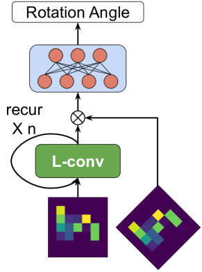
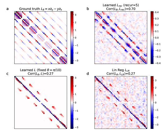
Figure 7: Learning the infinitesimal generator of $SO(2)$ Left shows the architecture for learning rotation angles between pairs of images. (a) shows the rotation generator calculated analytically using Shannon-Whittaker interpolation. (b) is the $\hat{L}$ learned using recursive L-conv learning rotation angle between a pair of images. (c) is an $L$ learned using a fixed small rotation angle $\theta=\pi/10$, and (d) shows $\hat{L}$ found using the numeric linear regression solution from the fixed angle data. (b) has the highest cosine correlation (0.70) with the ground truth, compared to 0.27 for $\hat{L}$ extracted using small angles.

Using fixed small angle

In the first experiment we try to learn a small rotation with angle $\theta=\pi/10$ using a single layer L-conv (Fig. 7,c). This experiment was already done in (Rao & Ruderman, 1999). The input is a random $7\times 7$ image ${\bm{f}}$ with pixels chosen in $[-.5,0.5)$. The output ${\bm{f}}^{\prime}$ is the same image rotated by $\theta$ using pytorch affine transform. Our training set contains 50,000 images., the test set was 10,000 images, batch size was 64. The code was implemented in pytorch and we used the Adam optimizer with learning rate $10^{-2}$. The experiments were run for 20 epochs. This problem is simply a linear regression with ${\bm{f}}^{\prime}=R{\bm{f}}=(I+{\epsilon}\hat{L}){\bm{f}}$. L-conv solves it using SGD and finds ${\epsilon}\hat{L}$. This problem can also be solved exactly using the solution to linear regression. Let $X=({\bm{f}}_{1},\dots\bm{f}_{N})$ and $Y=({\bm{f}}^{\prime}_{1},\dots\bm{f}^{\prime}_{N})$ be the matrix of all inputs and outputs, respectively. The rotation equation is $Y^{T}=RX^{T}$. Thus, the rotation matrix is given by $R=(Y^{T}X)(X^{T}X)^{-1}$. Figure 7 (c, d) shows the results of this experiment. The $L$ found using L-conv with SGD is much cleaner than the numerical linear regression solution $L_{LR}=(R-I)/\theta$. The loss becomes extremely small both on training and test data.

C.3 Learning rotation angle

In this experiment we have a pair of input images $({\bm{f}}_{n},R(\theta_{n}){\bm{f}}_{n})$, with $R(\theta)\in SO(2)$ (approximating 2D rotations). The two inputs differ by a finite rotation with angle $\theta_{n}\in[0,\pi/8)$. Th task is to learn the rotation angle $\theta_{n}$. For this task we use a recursive L-conv. We set $W^{0}=I$. The L-conv weight $\overline{{\epsilon}}$ is $m\times m$. To be able to encode multiple angles, we set $m=10$ and feed $10$ copies of the ${\bm{f}}_{n}$ as input ${\bm{h}}_{0}=[{\bm{f}}_{n}]\times 10$. We pass this through the same L-conv layer $t=3$ times as ${\bm{h}}_{i}=Q[{\bm{h}}_{i-1}]$. In the final layer, we first take the dot product of the final output ${\bm{h}}_{t}$ with the rotated input ${\bm{y}}_{n}=R(\theta){\bm{f}}_{n}$ to obtain ${\bm{g}}=\tanh\left({{\bm{y}}_{n}}^{T}{\bm{h}}_{t}\right)$. We then pass the output ${\bm{g}}\in\mathbb{R}^{m}$ through a fully-connected (FC) layer with $5$ nodes and tanh activation, and finally through a linear FC layer with one output to obtain the angle. The batch size was 16, Adam optimizer, learning rate $10^{-3}$, rest were default.

Despite being a much harder task than fitting a fixed angle rotation, the learned $\hat{L}$ of this experiment has the highest (0.70) cosine correlation with the ground truth $L_{\theta}$ (Fig. 7, b). Even though the architecture is rather complicated and L-conv is followed by two MLP layers, the $\hat{L}$ in L-conv learns the infinitesimal generator of rotations very well. We also conducted experiments with larger random images $(20\times 20)$ and larger angles of rotation $\theta_{n}\in[0,\pi/4)$ (Fig. 8). While the accuracy of learning the angles is still pretty good (Fig. 8, e,test loss $2.7\times 10^{-4}$) the larger angles result in less correlation between the learned $\hat{L}$ and the ground truth $L_{\theta}$ (Fig. 8, b, correlation $0.12$ with 8 times recurrence). The learned $\hat{L}$ is closer to a finite angle rotation. This may be because the with small number of recurrences the network found small but finite rotations approximate larger rotations better than using a true infinitesimal generator.

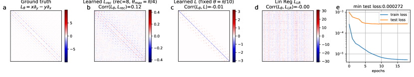
Figure 8: Learning $\hat{L}$ via larger rotation angles for larger images. This time the correlation with ground truth $L_{\theta}$ is much less, but accuracy is still very good.

Appendix D Experiments on Images

To understand precisely how L-conv performs in comparison with CNN and other baselines, we conduct a set of carefully designed experiments. Defining pooling for L-conv merits more research. Without pooling, we cannot use L-conv in state-of-the-art models for problems such as image classification. Therefore, we use the simplest possible models in our experiments: one or two L-conv, or CNN, or FC layers, followed by a classification layer. We do not use any other operations such as dropout or batch normalization in any of the experiments.

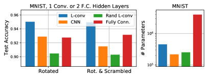
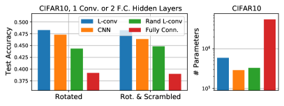
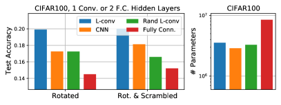
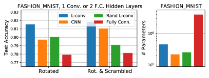
Figure 9: Results on four datasets with two variant: “Rotated” and “Rotated and scrambled”. In all cases L-conv performs best. On MNIST, FC and CNN come close, but using 5x more parameters.

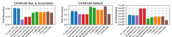
Figure 10: Comparison of one and two layer performance of L-conv (blue), CNN without pooling (orange), CNN with Maxpooling after each layer (green), fully connected (FC) with structure similar to L-conv (red), Lie-Conv (Finzi) Finzi et al. (2020) (brown), and shallow FC, which has a single hidden layer with width such that the total number of parameters matches L-conv (purple). The labels indicate number of layers, layer architecture and number of filters (e.g. “2 L-conv (32)” means two layers of L-conv with 32 filters followed by one classification layer). Left and middle plots show test accuracies on CIFAR100 with rotated and scrambled images, and on the original CIFAR100 dataset, respectively. The plot on the right shows the number of parameters in each model, which is the same for the two datasets.

Test Datasets We use four datasets: MNIST, CIFAR10, CIFAR100, and FashionMNIST. To test the efficiency of L-conv in dealing with hidden or unfamiliar symmetries, we conducted our tests on two modified versions of each dataset: 1) Rotated: each image rotated by a random angle (no augmentation); 2) Rotated and Scrambled: random rotations are followed by a fixed random permutation (same for all images) of pixels. We used a 80-20 training test split on 60,000 MNIST and FashionMNIST, and on 50,000 CIFAR10 and CIFAR100 images. Scrambling destroys the correlations existing between values of neighboring pixels, removing the locality of features in images. As a result, CNN need to encode more patterns, as each image patch has a different correlation pattern.

Test Model Architectures We conduct controlled experiments, with one (Fig. 9) or two (Fig. 10) hidden layers being either L-conv or a baseline, followed by a classification layer. For CNN, L-conv and L-conv with random $L_{i}$, we used $n_{f}=m_{l}=32$ for number of output filters (i.e. output dimension of $W^{i}$). For CNN we used $3\times 3$ kernels and equivalently used $n_{L}=9$ for the number of $L_{i}$ in L-conv and random L-conv. We also used “LieConv” Finzi et al. (2020) as a baseline (Fig. 10, brown). We used the default $k=256$ in LieConv, which yields comparable number of parameters to our other models. For the symmetry group in LieConv we used $SE(3)$. We also used the default ResNet architecture provided by Finzi et al. (2020) for both the one and two layer experiments. We turned off batch normalization, consistent with other experiments. We encode $L_{i}$ as sparse matrices $L_{i}=U_{i}V_{i}$ with hidden dimension $d_{h}=16$ in Fig. 9 and $d_{h}=8$ in Fig. 10, showing that very sparse $L_{i}$ can perform well. The weights $W^{i}$ are each $m_{l}\times m_{l+1}$ dimensional. The output of the L-conv layer is $d\times m_{l+1}$. As mentioned above, we use two FC baselines. The FC in Fig. 9 and FC($\sim$L-conv) in Fig. 10 mimic L-conv, but lacks weight-sharing. The FC weights are $W=ZV$ with $V$ being $(n_{L}d_{h})\times d$ and $Z$ being $(m_{l+1}\times d)\times d_{h}$. For “FC (shallow)” in Fig. 10, we have one wide hidden layer with $u=n_{L-conv}/(mdc)$, where $n_{L-conv}$ is the total number of parameters in the L-conv model, $m$ and $c$ the input and output channels, and $d$ is the input dimension. We experimented with encoding $L_{i}$ as multi-layer perceptrons, but found that a single hidden layer with linear activation works best. We also conduct tests with two layers of L-conv, CNN and FC (Fig. 10), with each L-conv, CNN and FC layer as descried above, except that we reduced the hidden dimension in $L_{i}$ to $d_{h}=8$.

Baselines We compare L-conv against four baselines: CNN, random $L_{i}$, fully connected (FC) and LieConv. Using CNN or $SE(3)$ LieConv on scrambled images amounts to using poor inductive bias in designing the architecture. Similarly, random, untrained $L_{i}$ is like using bad inductive biases. Testing on random $L_{i}$ serves to verify that L-conv’s performance is not due to the structure of the architecture, and that the $L_{i}$ in L-conv really learn patterns in the data. Finally, to verify that the higher parameter count in L-conv is not responsible for the high performance, we construct two kinds of FC models. The first type (“Fully Conn.” in Fig. 9 and “FC ($\sim$ L-conv)” in Fig. 10) is a multilayer FC network with the same input ($d\times m_{0}$), hidden ($k\times n_{L}$ for low-rank $L_{i}$) and output ($d\times m_{1}$) dimensions as L-conv, but lacking the weight-sharing, leading to much larger number parameters than L-conv. The second type (“FC (shallow)” in Fig. 10) consists of a single hidden layer with a width such that the total number of model parameters match L-conv.

Results Fig. 9 shows the results for single layer experiments. On all four datasets both in the rotated and the rotated and scrambled case L-conv performed considerably better than CNN and the baselines. Compared to CNN, L-conv naturally requires extra parameters to encode $L_{i}$, but low-rank encoding with rank $d_{h}\ll d$ only requires $O(d_{h}d)$ parameters, which can be negligible compared to FC layers. We observe that FC layers consistently perform worse than L-conv, despite having much more parameters than L-conv. We also find that not training the $L_{i}$ (“Rand L-conv”) leads to significant performance drop. We ran tests on the unmodified images as well (Supp. Fig 12), where CNN performed best, but L-conv trails closely behind CNN.

Additional experiments testing the effect of number of layers, number of parameters and pooling are shown in Fig. 10. On CIFAR100, we find that both FC configurations, FC($\sim$L-conv) and FC(shallow) consistently perform worse than L-conv, evidence that L-conv’s performance is not due to its extra parameters. L-conv outperforms all other tested models on rotated and scrambled CIFAR100, including LieConv. Without pooling, we observe that both L-conv and CNN do not benefit from adding a second layer. On the default CIFAR100 dataset, one and two layer CNN with max-pooling perform significantly better than L-Conv. Two Layer $SE(3)$ LieConv (labelled “2 Finzi (256)”) performs best on default CIFAR100, but not on the scrambled and rotated version. This is expected, as the symmetries of the latter are masked by the scrambling. This is where the benefit of our model becomes evident, namely cases where the data may have hidden or unfamiliar symmetries. We also verified that the higher performance of L-conv compared to CNN is not due to higher number number of parameters (Appendix D.2)

D.1 Details of experiments

Hardware and Implementation

We implemented L-conv in Keras and Tensorflow 2.2 and ran our tests on a system with a 6 core Intel Core i7 CPU, 32GB RAM, and NVIDIA Quadro P6000 (24GB RAM) GPU. The L-conv layer did not require significantly more resources than CNN and ran only slightly slower.

D.2 Additional Experiments

Matching number of parameters in CNN To verify that the difference in the number of parameters between CNN and L-conv was not responsible for the improved performance, we ran experiment where we allowed the kernel-size of L-conv and CNN to differ and tried to match the number of parameters between the two. Fig. 11 shows that on rotated and scrambled MNIST L-conv still performs better than CNN even after the latter has been allowed to have the same or more number of parameters than L-conv.

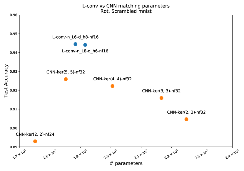
Figure 11: Matching number of parameters in CNN and L-conv, we observe that L-conv still performs better on Rotated and Scrambled MNIST.

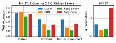
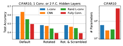
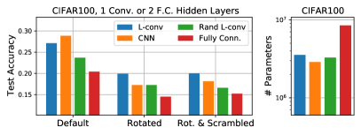
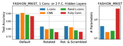
Figure 12: Test results on four datasets with three variant: “Default” (unmodified dataset), “Rotated” and “Rotated and scrambled”. On the Default dataset, CNN performs best, but L-conv is always the second best. For Rotated and Rot. & Scrambled, in all cases L-conv performed best. In MNIST, FC and CNN layers come close, but using 5x more parameters.

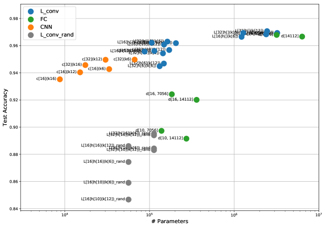
Figure 13: Training low-rank L-conv layer during training.

In Figure 13 we compare the performance of a single layer of L-conv on a classification task on scrambled rotated MNIST, where pixels have been permuted randomly and images have been rotated between $-90$ to $+90$ degrees. The models consisted of a final classification layer preceded by either one L-conv (blue), or one CNN (orange), or multiple fully-connected (FC, green) layers with similar number of neurons as the L-conv, but without weight sharing. We see that most L-conv configurations had the highest performance without a too many trainable parameters. Note that, parameters in FC layers are much higher than comparable L-conv, but yield worse results. The dots are labeled to show the configurations, with $L[32]h[6](k[6])$ meaning $k=6$ as number of $L_{i}$, 32 output filters, and $h=6$ hidden dimensions for low-rank encoding of $L_{i}$. The y-axis shows the test accuracy and the x-axis the number of trainable parameters. The grey lines show the performance of L-conv with fixed random $L_{i}$, but trainable shared wights, showing that indeed the learned $L_{i}$ improve the performance quite significantly.

References

- Anselmi et al. (2019) Anselmi, F., Evangelopoulos, G., Rosasco, L., and Poggio, T. Symmetry-adapted representation learning. Pattern Recognition, 86:201–208, 2019.
- Benton et al. (2020) Benton, G., Finzi, M., Izmailov, P., and Wilson, A. G. Learning invariances in neural networks. arXiv preprint arXiv:2010.11882, 2020.
- Bogatskiy et al. (2020) Bogatskiy, A., Anderson, B., Offermann, J., Roussi, M., Miller, D., and Kondor, R. Lorentz group equivariant neural network for particle physics. In International Conference on Machine Learning, pp. 992–1002. PMLR, 2020.
- Bronstein et al. (2021) Bronstein, M. M., Bruna, J., Cohen, T., and Veličković, P. Geometric deep learning: Grids, groups, graphs, geodesics, and gauges. arXiv preprint arXiv:2104.13478, 2021.
- Cohen & Welling (2014) Cohen, T. and Welling, M. Learning the irreducible representations of commutative lie groups. In International Conference on Machine Learning, pp. 1755–1763, 2014.
- Cohen & Welling (2016a) Cohen, T. and Welling, M. Group equivariant convolutional networks. In International conference on machine learning, pp. 2990–2999, 2016a.
- Cohen et al. (2019a) Cohen, T., Weiler, M., Kicanaoglu, B., and Welling, M. Gauge equivariant convolutional networks and the icosahedral cnn. In International Conference on Machine Learning, pp. 1321–1330. PMLR, 2019a.
- Cohen & Welling (2016b) Cohen, T. S. and Welling, M. Steerable cnns. 2016b.
- Cohen et al. (2018) Cohen, T. S., Geiger, M., Köhler, J., and Welling, M. Spherical cnns. In International Conference on Learning Representations, 2018.
- Cohen et al. (2019b) Cohen, T. S., Geiger, M., and Weiler, M. A general theory of equivariant cnns on homogeneous spaces. In Advances in Neural Information Processing Systems, pp. 9142–9153, 2019b.
- Cybenko (1989) Cybenko, G. Approximation by superpositions of a sigmoidal function. Mathematics of control, signals and systems, 2(4):303–314, 1989.
- Finzi et al. (2020) Finzi, M., Stanton, S., Izmailov, P., and Wilson, A. G. Generalizing convolutional neural networks for equivariance to lie groups on arbitrary continuous data. arXiv preprint arXiv:2002.12880, 2020.
- Finzi et al. (2021) Finzi, M., Welling, M., and Wilson, A. G. A practical method for constructing equivariant multilayer perceptrons for arbitrary matrix groups. arXiv preprint arXiv:2104.09459, 2021.
- Gilmer et al. (2017) Gilmer, J., Schoenholz, S. S., Riley, P. F., Vinyals, O., and Dahl, G. E. Neural message passing for quantum chemistry. In International Conference on Machine Learning, pp. 1263–1272. PMLR, 2017.
- Hall (2015) Hall, B. Lie groups, Lie algebras, and representations: an elementary introduction, volume 222. Springer, 2015.
- Hartford et al. (2018) Hartford, J., Graham, D., Leyton-Brown, K., and Ravanbakhsh, S. Deep models of interactions across sets. In International Conference on Machine Learning, pp. 1909–1918. PMLR, 2018.
- Hornik et al. (1989) Hornik, K., Stinchcombe, M., and White, H. Multilayer feedforward networks are universal approximators. Neural networks, 2(5):359–366, 1989.
- Kipf & Welling (2016) Kipf, T. N. and Welling, M. Semi-supervised classification with graph convolutional networks. arXiv preprint arXiv:1609.02907, 2016.
- Kondor & Trivedi (2018) Kondor, R. and Trivedi, S. On the generalization of equivariance and convolution in neural networks to the action of compact groups. arXiv preprint arXiv:1802.03690, 2018.
- Kondor et al. (2018) Kondor, R., Lin, Z., and Trivedi, S. Clebsch–gordan nets: a fully fourier space spherical convolutional neural network. In Advances in Neural Information Processing Systems, pp. 10117–10126, 2018.
- Kunin et al. (2020) Kunin, D., Sagastuy-Brena, J., Ganguli, S., Yamins, D. L., and Tanaka, H. Neural mechanics: Symmetry and broken conservation laws in deep learning dynamics. arXiv preprint arXiv:2012.04728, 2020.
- Landau (2013) Landau, L. D. The classical theory of fields, volume 2. Elsevier, 2013.
- LeCun et al. (1989) LeCun, Y., Boser, B., Denker, J. S., Henderson, D., Howard, R. E., Hubbard, W., and Jackel, L. D. Backpropagation applied to handwritten zip code recognition. Neural computation, 1(4):541–551, 1989.
- LeCun et al. (1998) LeCun, Y., Bottou, L., Bengio, Y., and Haffner, P. Gradient-based learning applied to document recognition. Proceedings of the IEEE, 86(11):2278–2324, 1998.
- Lee et al. (2009) Lee, J. M., Chow, B., Chu, S.-C., Glickenstein, D., Guenther, C., Isenberg, J., Ivey, T., Knopf, D., Lu, P., Luo, F., et al. Manifolds and differential geometry. Topology, 643:658, 2009.
- Polyakov (2018) Polyakov, A. M. Gauge fields and strings. Routledge, 2018.
- Rao & Ruderman (1999) Rao, R. P. and Ruderman, D. L. Learning lie groups for invariant visual perception. In Advances in neural information processing systems, pp. 810–816, 1999.
- Ravanbakhsh (2020) Ravanbakhsh, S. Universal equivariant multilayer perceptrons. arXiv preprint arXiv:2002.02912, 2020.
- Ravanbakhsh et al. (2017) Ravanbakhsh, S., Schneider, J., and Poczos, B. Equivariance through parameter-sharing. In Proceedings of the 34th International Conference on Machine Learning-Volume 70, pp. 2892–2901. JMLR. org, 2017.
- Schaub et al. (2020) Schaub, M. T., Benson, A. R., Horn, P., Lippner, G., and Jadbabaie, A. Random walks on simplicial complexes and the normalized hodge 1-laplacian. SIAM Review, 62(2):353–391, 2020.
- Sohl-Dickstein et al. (2010) Sohl-Dickstein, J., Wang, C. M., and Olshausen, B. A. An unsupervised algorithm for learning lie group transformations. arXiv preprint arXiv:1001.1027, 2010.
- Wang et al. (2020) Wang, R., Walters, R., and Yu, R. Incorporating symmetry into deep dynamics models for improved generalization. In International Conference on Learning Representations, 2020.
- Weiler & Cesa (2019) Weiler, M. and Cesa, G. General e (2)-equivariant steerable cnns. In Advances in Neural Information Processing Systems, pp. 14334–14345, 2019.
- Weiler et al. (2018a) Weiler, M., Geiger, M., Welling, M., Boomsma, W., and Cohen, T. S. 3d steerable cnns: Learning rotationally equivariant features in volumetric data. In Advances in Neural Information Processing Systems, pp. 10381–10392, 2018a.
- Weiler et al. (2018b) Weiler, M., Hamprecht, F. A., and Storath, M. Learning steerable filters for rotation equivariant cnns. In Proceedings of the IEEE Conference on Computer Vision and Pattern Recognition, pp. 849–858, 2018b.
- Weinberg (1995) Weinberg, S. The quantum theory of fields, volume 3. Cambridge university press, 1995.
- Whitaker (1915) Whitaker, E. On the functions which are represented by the expansion of interpolating theory. In Proc. Roy. Soc. Edinburgh, volume 35, pp. 181–194, 1915.
- Worrall et al. (2017) Worrall, D. E., Garbin, S. J., Turmukhambetov, D., and Brostow, G. J. Harmonic networks: Deep translation and rotation equivariance. In Proceedings of the IEEE Conference on Computer Vision and Pattern Recognition, pp. 5028–5037, 2017.
- Zaheer et al. (2017) Zaheer, M., Kottur, S., Ravanbakhsh, S., Poczos, B., Salakhutdinov, R. R., and Smola, A. J. Deep sets. In Advances in neural information processing systems, pp. 3391–3401, 2017.
- Zhou et al. (2020) Zhou, A., Knowles, T., and Finn, C. Meta-learning symmetries by reparameterization. arXiv preprint arXiv:2007.02933, 2020.