Performance-Efficiency Trade-offs
in Unsupervised Pre-training
for Speech Recognition

Abstract

This paper is a study of performance-efficiency trade-offs in pre-trained models for automatic speech recognition (ASR). We focus on wav2vec 2.0, and formalize several architecture designs that influence both the model performance and its efficiency. Putting together all our observations, we introduce SEW (Squeezed and Efficient Wav2vec), a pre-trained model architecture with significant improvements along both performance and efficiency dimensions across a variety of training setups. For example, under the 100h-960h semi-supervised setup on LibriSpeech, SEW achieves a 1.9x inference speedup compared to wav2vec 2.0, with a 13.5% relative reduction in word error rate. With a similar inference time, SEW reduces word error rate by 25–50% across different model sizes.

1 Introduction

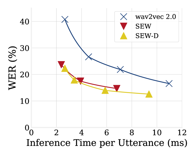
Figure 1: Word error rate (WER) and average utterance inference time on LibriSpeech (dev-other) of wav2vec 2.0 and our SEW and SEW-D models fine-tuned with 100h labeled data for 100K updates.

Recently, there is significant interest in self-supervised pre-training using unlabeled audio data to learn versatile feature representations, that are subsequently fine-tuned on task-specific annotated audio (Zhang et al., 2020b; Wang et al., 2021b; Xu et al., 2020a; Pepino et al., 2021). This follows similar trends in natural language processing (NLP; Devlin et al., 2018; Liu et al., 2019; He et al., 2020) and computer vision (CV; He et al., 2019; Chen et al., 2020; Grill et al., 2020). Maybe the most prominent example of this class of models is wav2vec 2.0 (W2V2; Baevski et al., 2020b), which achieves competitive word error rate (WER) following fine-tuning on only ten minutes of transcribed (labeled) data, when prior supervised approaches often require nearly a thousand hours. If recent developments in NLP and CV are any indication, the importance of such pre-trained audio models that are fine-tuned on expert tasks will only increase. Indeed, W2V2 has already been studied with focus on the impact of pre-training data (Conneau et al., 2020; Hsu et al., 2021), pre-training task (Hsu et al., 2020), or combination with pseudo labelling (Xu et al., 2020a; Zhang et al., 2020b).

In this paper, we study W2V2’s model design, and possible trade-offs between its components. Our focus is on efficiency for practical applications, rather than extending the model. As W2V2-type models become increasingly common, understanding their efficiency trade-offs is critical for transferring their benefits from the lab to the real world, where any increase in efficiency can substantially reduce the inference costs and energy footprints across a plethora of real world applications.

We study several aspects of the W2V2 model. We focus on automatic speech recognition (ASR), while retaining the standard pre-training and few-sample fine-tuning setup. First, we study how the temporal resolution of the network trades-off performance and efficiency, and show that using different resolutions for computing pre-trained representations and ASR decoding significantly reduces inference time, while retaining similar performance. Second, we propose an efficient family of waveform feature extractors, which achieves similar performance with half the inference time as the original W2V2 extractor. Finally, we study the impact of shifting model expressivity between different parts of the network. We observe that it is better to assign more parameters to later parts in the pre-trained network, compared to increasing capacity closer to the input waveform. We also see that increasing the expressivity of the pre-training predictor heads increases performance, while not influencing downstream-task computation as these heads are discarded.

We combine our observations to propose two models: SEW (Squeezed and Efficient Wav2vec) and SEW-D (SEW with disentangled attention (He et al., 2020)). We pre-train SEW and SEW-D on 960 hours of unlabelled audio from the LibriSpeech dataset (Panayotov et al., 2015), and fine-tune with multiple ASR tasks. SEW yields a significantly better performance-efficiency trade-off than the original W2V2. For example, with 100h labeled data, compared to a W2V2-tiny model, SEW reduces the LibriSpeech test-clean WER from 22.8% to 10.6% while being slightly faster, even outperforming a larger W2V2 model with 12.8% WER. Compared to the official W2V2-large release, our best SEW-D-base+ achieves 2.7$\times$ and 3.2$\times$ speed-ups for inference and pre-training with comparable WER using half of the number of parameters. Compared to W2V2-base, our SEW-D-mid achieves 1.9$\times$ inference speed-up with a 13.5% relative reduction in WER. Figure 1 shows the performance-efficiency trade-offs with various model size. SEW-D outperforms W2V2 in most pre-training settings, when experimenting with LibriSpeech (Panayotov et al., 2015), Ted-lium 3 (Hernandez et al., 2018), VoxPopuli (Wang et al., 2021a), and Switchboard (Godfrey and Holliman, 1993) datasets. Pre-trained models and code are available at https://github.com/asappresearch/sew.

2 Related Work

Unsupervised Audio Representation Learning

Contrastive predictive coding (CPC) is a general unsupervised learning method for speech, vision, text, and reinforcement learning (van den Oord et al., 2018). When applied to speech, it uses past audio to predict the future audio, similar to language modeling (Mikolov et al., 2010; Dauphin et al., 2017; Kaplan et al., 2020) but with contrastive loss. Wav2vec (Schneider et al., 2019) further improves the CPC model architecture design and focuses on unsupervised pre-training for end-to-end automatic speech recognition. Roughly speaking, wav2vec includes a feature extractor that generates a sequence of vectors from raw waveform audio, and a context network that encodes the features from the recent past to predict the features in the immediate future. This context network is only used to learn useful feature representations, and is typically discarded after pre-training. Recently, Baevski et al. (2020a) introduced vq-wav2vec and a combination of vq-wav2vec with a discrete BERT-like model (Devlin et al., 2019; Baevski et al., 2019). W2V2 (Baevski et al., 2020b) combines vq-wav2vec and the BERT-like model into an end-to-end setup, where the BERT portion functions as the context network, but not discarded. More recently, Hsu et al. (2020) propose HuBERT and show that W2V2 can be pre-trained with clustered targets instead of contrastive objectives. Besides ASR-focused works, there is significant interest in learning representations for other speech tasks (Synnaeve and Dupoux, 2016; Chung et al., 2018; Chuang et al., 2019; Song et al., 2019), music (Yang et al., 2021; Zhao and Guo, 2021), and general audio (Saeed et al., 2021; Gong et al., 2021; Niizumi et al., 2021; Wang et al., 2021c).

End-to-end Automatic Speech Recognition (ASR)

As large datasets and fast compute become available, end-to-end ASR models (Amodei et al., 2016; Zhang et al., 2020b) increasingly achieve state-of-the-art results, outperforming HMM-DNN hybrid systems (Abdel-Hamid et al., 2012; Hinton et al., 2012). End-to-end ASR models can be roughly categorized into three main types: connectionist temporal classification (CTC; Graves et al., 2013), RNN transducers (RNN-T; Graves, 2012; Han et al., 2020; Gulati et al., 2020), and sequence-to-sequence (a.k.a. Listen, Attend and Spell models) (Seq2seq; Chan et al., 2016; Dong et al., 2018; Watanabe et al., 2018). CTC models are extremely fast for batch decoding; RNN-T variants are often used in real-time systems; Seq2seq models are more popular in offline settings. Recently, and following success on NLP tasks, there is a transition in speech processing towards the Transformer architecture (Vaswani et al., 2017; Dong et al., 2018) and its variants (Zhang et al., 2020a; Baevski et al., 2020b; Gulati et al., 2020; Zhang et al., 2020b; Yeh et al., 2019).

3 Technical Background: Wav2Vec 2.0 (W2V2)

W2V2 is made of a waveform feature extractor that generates a sequence of continuous feature vectors, each encoding a small segment of audio, and a context network that maps these vectors to context-dependent representations.

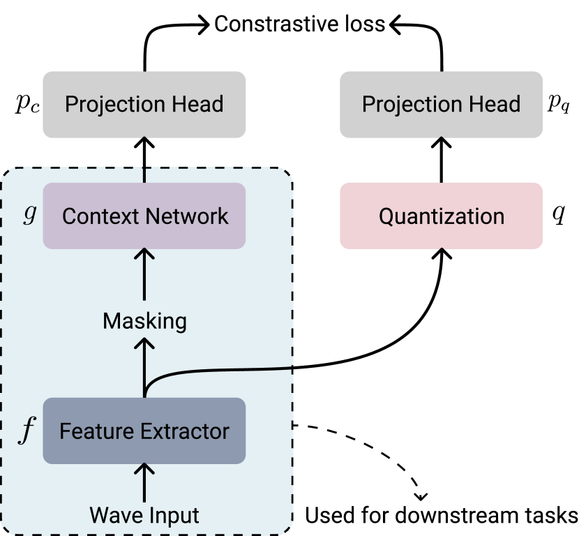
Figure 2: Wav2vec 2.0 framework.

During pre-training, some of the features are masked out, and are not seen by the context network. In parallel, the pre-masking features are discretized as prediction targets. The context network aims to discriminate the discretized version of the original features at the masked positions from a pool of negative samples using the InfoNCE loss (van den Oord et al., 2018).

Figure 2 shows the W2V2 framework, including (a) a feature extractor, (b) a context network, (c) an optional quantization module, and (d) two projection heads.

Wave Feature Extractor (WFE)

The wave feature extractor $f(\cdot)$ encodes and downsamples the raw waveform audio inputs ${\mathbf{X}}=({\bm{x}}_{1},...,{\bm{x}}_{T_{\text{input}}})\in\mathbb{R}^{T_{\text{input}}\times d_{\text{input}}}$ ($d_{\text{input}}=1$ for single-channel audio) into an array of feature vectors ${\mathbf{Z}}=f({\mathbf{X}})=({\bm{z}}_{1},...,{\bm{z}}_{T})\in\mathbb{R}^{T\times\mathbb{R}^{d_{\text{feat}}}}$. For example, W2V2 maps 16KHz audio sequences to 50Hz frames using a convolutional WFE with receptive field size of 400 and stride size of 320. Each feature vector encodes the raw signals within a 25ms ($=1000/16000*400$) window with a stride size 20ms ($=1000/16000*320$). The reduced sequence length is $T=\frac{T_{\text{input}}-400}{320}+1=\frac{T_{\text{input}}-80}{320}$.

Context Network

The context network $g(\cdot)$ follows a similar principle as masked language models in NLP (e.g., BERT (Devlin et al., 2018) or RoBERTa (Liu et al., 2019)). During pre-training, each $z_{t}$ is masked and replaced with a trainable mask vector ${\bm{m}}$ with a predefined probability $p$. To illustrate, ${\mathbf{Z}}=({\bm{z}}_{1},{\bm{z}}_{2},{\bm{z}}_{3},{\bm{z}}_{4},{\bm{z}}_{5},{\bm{z}}_{6},...,{\bm{z}}_{T})$ can become ${\mathbf{Z}}^{\prime}=({\bm{z}}_{1},{\bm{m}},{\bm{m}},{\bm{z}}_{4},{\bm{m}},{\bm{z}}_{6},...,{\bm{z}}_{T})$. The context network maps this masked sequence to a sequence of contextual representations ${\mathbf{C}}=g({\mathbf{Z}}^{\prime})=({\bm{c}}_{1},...,{\bm{c}}_{T})\in\mathbb{R}^{T\times d_{\text{feat}}}$ to incorporate context information. Even if ${\bm{z}}_{t}$ is masked and replaced with ${\bm{m}}$, we anticipate that ${\bm{c}}_{t}$ can recover the information in ${\bm{z}}_{t}$ because it contains information from surrounding, not-masked input vectors. The context network is usually implemented with a Transformer architecture (Vaswani et al., 2017; Gulati et al., 2020).

Quantization Module

The quatization module $q(\cdot)$ maps each unmasked vector ${\bm{z}}_{t}$ into a quantized form ${\bm{q}}_{t}=q({\bm{z}}_{t})\in\mathbb{R}^{d_{\text{feat}}}$ for each masked position $t$. Quantized ${\bm{q}}_{t}$’s are the prediction targets. The quantization module is based on Gumbel softmax with straight-through estimator (Gumbel, 1954; Jang et al., 2016; Maddison et al., 2014). There are $G$ codebooks and each codebook has $V$ entries, giving $G\times V$ vectors ${\bm{e}}_{g,v}\in\mathbb{R}^{\frac{d_{\text{feat}}}{G}}$ where $g\in\{1,...,G\},v\in\{1,...,V\}$. For each group $g$, the probability of assigning ${\bm{z}}_{t}$ to the $v$-th entry is $p_{g,v}=\frac{\exp({\bm{W}}^{g}_{v}\cdot{\bm{z}}_{t}/\tau_{Q})}{\sum_{v^{\prime}=1}^{V}\exp({\bm{W}}^{g}_{v^{\prime}}\cdot{\bm{z}}_{t}/\tau_{Q})}$, where ${\bm{W}}^{g}\in\mathbb{R}^{V\times d_{\text{feat}}}$ is a trainable matrix and $\tau_{Q}$ is the quantization temperature. For each group $g$, ${\bm{z}}_{t}$ is assigned to the $v_{g}^{*}$-th entry where $v_{g}^{*}=\operatorname*{arg\,max}_{v}p_{g,v}$. The corresponding embedding vectors $({\bm{e}}_{1,v_{1}^{*}},...,{\bm{e}}_{G,v_{G}^{*}}$) are concatenated to a single vector ${\bm{q}}_{t}\in\mathbb{R}^{d_{\text{feat}}}$, and constitutes a quantized feature sequence ${\mathbf{Q}}=({\bm{q}}_{1},...,{\bm{q}}_{T})\in\mathbb{R}^{T\times d_{\text{feat}}}$.

Projection Heads

Two linear projection heads $p_{c}(\cdot)$ and $p_{q}(\cdot)$ reduce the dimensionality of ${\mathbf{C}}$ and ${\mathbf{Q}}$. For a ${\bm{z}}_{t}$ that is masked and replaced with ${\bm{m}}$, we want $p_{c}({\bm{c}}_{t})\in\mathbb{R}^{d_{\text{proj}}}$ to be similar to $p_{q}({\bm{q}}_{t})\in\mathbb{R}^{d_{\text{proj}}}$. Baevski et al. (2020b) do not separate between $p_{c}$ and $g$ or $p_{q}$ and $q$ in their original notations. However, we keep the distinctions, as they serve different roles and are discarded before downstream fine-tuning.

Pre-training Objective

W2V2 combines contrastive and diversity losses in the pre-training loss:

$${\mathcal{L}}={\mathcal{L}}_{m}+\alpha{\mathcal{L}}_{d}\;\;.$$ (1)

The goal of the contrastive loss ${\mathcal{L}}_{m}$ is to make the projected outputs $p_{c}({\bm{c}}_{t})$ close to $p_{q}({\bm{q}}_{t})$ and far away from any other $p_{q}({\bm{q}}_{t^{\prime}})$, where ${\bm{z}}_{t}$ is masked and $t^{\prime}$ is any other position in the same sequence. W2V2 uses an InfoNCE loss (van den Oord et al., 2018):

$${\mathcal{L}}_{m}=\mathbb{E}_{t\text{\ is masked}}\left[-\log\frac{\exp(\mathrm{sim}(p_{c}({\bm{c}}_{t}),p_{q}({\bm{q}}_{t}))/\kappa)}{\sum_{{\bm{q}}_{t^{\prime}}\in\mathbb{Q}}\exp(\mathrm{sim}(p_{c}({\bm{c}}_{t}),p_{q}({\bm{q}}_{t^{\prime}}))/\kappa)}\right],$$ (2)

with $\mathrm{sim}({\bm{a}},{\bm{b}})=\frac{{\bm{a}}^{\top}{\bm{b}}}{\left\lVert{\bm{a}}\right\rVert\left\lVert{\bm{b}}\right\rVert}$, $\mathbb{Q}$ is a set containing the positive sample ${\bm{q}}_{t}$ and $K$ negative samples, and $\kappa$ is the temperature. The expectation is computed over masked positions only. The diversity loss ${\mathcal{L}}_{d}$ prevents the quantization module from collapsing to a trivial mapping (e.g., by collapsing all inputs to a single discrete code). It encourages the quantization probability $p_{g,v}$ to be evenly distributed:

$${\mathcal{L}}_{d}=\mathbb{E}_{t}\left[1-\frac{1}{GV}\sum_{g=1}^{G}\exp\left(-\sum_{v=1}^{V}p_{g,v}\log p_{g,v}\right)\right].$$ (3)

4 Exploring Model Design Trade-offs

4.1 Experimental Setup

We use the official W2V2 implementation in fairseq (Ott et al., 2019), with the hyper-parameters of W2V2-base (Baevski et al., 2020b). We describe key hyper-parameters; the linked configuration files provide the full details.

Pre-training

We use the LibriSpeech (CC BY 4.0) (Panayotov et al., 2015) 960h training data for unsupervised pre-training, leaving 1% as validation set for pre-training. We use the same hyperparameters as W2V2-base (Appendix B). To speed up and reduce the cost of our experiments, we pre-train all models for 100K updates similar to Hsu et al. (2020). All experiments use an AWS p3.16xlarge instance with 8 NVIDIA V100 GPUs and 64 Intel Xeon 2.30GHz CPU cores. Because Baevski et al. (2020b) use 64 GPUs, we set gradient accumulation steps to 8 to simulate their 64-GPU pre-training with 8 GPUs.

Fine-tuning

We add a linear classifier to the top of the context network and fine-tune the model using a CTC objective on LibriSpeech train-clean 100h set for 80K updates using the same set of hyper-parameters as W2V2-base (Appendix B).

Evaluation

We use CTC greedy decoding (Graves et al., 2006) for all experiments because it is faster than Viterbi decoding (Viterbi, 1967) and we do not find any WER differences between the two using baseline W2V2 models (Appendix D). We use LibriSpeech dev-other for validation, and hold out test-clean and test-other as test sets. We consider three metrics to evaluate model efficiency and performance: pre-training time, inference time, and WER (word error rate). All evaluation is done on a NVIDIA V100 GPU with FP32 operations, unless specified otherwise. When decoding with a language model (LM), we use the official 4-gram LM and wav2letter (Collobert et al., 2016) decoder with the default LM weight 2, word score -1, and beam size 50. Reducing the inference time with LM is an important direction for future work, as the wav2letter decoder is the bottleneck and is at least 3$\times$ slower than W2V2-base (Appendix D).

4.2 Depth vs. Width

The smallest W2V2 model is W2V2-base with 94M parameters and is already relatively large compared to other ASR models (Han et al., 2020; Gulati et al., 2020). We study two strategies of changing the context network Transformer to reduce the model size and speed up the model, potentially at cost to performance: reducing model depth by using fewer Transformer layers or reducing model width by using smaller hidden state size in the Transformer. When reducing the hidden size, we fix the head dimension to 64. For example, a 12-head 768$d$ Transformer would be scaled down to a 4-head 256$d$ Transformer. The hidden size of the feed-forward network is always 4x as wide as the Transformer width. We also scale down the wave feature extractor to ensure that its width is not larger than the width of the Transformer. For fairness of comparison, the depth counterpart uses the same wave feature extractor as well.

Figure 4 shows the performance-efficiency trade-offs of scaling down the depth or width of the model. Scaling down the width achieves better performance-efficiency compared to scaling down the depth; a deep and narrow model is more favorable than a shallow and wide model. These narrow models serve as the baselines for our following experiments.

4.3 Temporal Resolution vs. Model Size

The wave feature extractor of W2V2 down-samples the raw audio to 50Hz frames with a stride size of 20ms, reducing the sequence length by a factor of 320 (section 3). However, even lower resolutions are common in prior end-to-end ASR approaches. For example, several methods (Han et al., 2020; Gulati et al., 2020) use log-mel filterbank features with a stride of 10ms (100Hz) and down-sample them to 40ms (25Hz) with two layers of strided convolutions. The result is halving the sequence length, and reducing the computation and memory footprint of the context network. Reducing the sequence length may allow increasing the model size with the same computation costs.

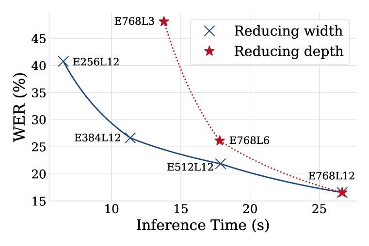
Figure 3: LibriSpeech dev-other WER versus inference time (with 100h labeled data). Reducing the width of the model (E768 $\rightarrow$ E512 $\rightarrow$ E384 $\rightarrow$ E256) achieves better performance-efficiency trade-off compared to reducing the depth (L12 $\rightarrow$ L6 $\rightarrow$ L3).

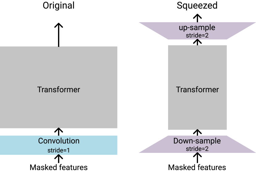
Figure 4: Original vs. squeezed context network. The sequence length is halved by the down-sampling layer.

	Resolution				Inference	dev-other
Model	Encode	Mask Pred.	CTC	# Param.	Time (s)	WER	(+LM)
W2V2 E256L12 (baseline)	50Hz	50Hz	50Hz	11.06M	7.5$\pm$0.04	40.7	23.4
W2V2 E384L12 25Hz	25Hz	25Hz	25Hz	23.76M	6.7$\pm$0.02	33.1	20.5
+ FT upsample	25Hz	25Hz	50Hz	24.06M	6.7$\pm$0.02	31.5	18.5
Sq-W2V E384L12	25Hz	50Hz	50Hz	23.92M	7.0$\pm$0.01	29.9	17.5
W2V2 E384L12 (WER lower bound)	50Hz	50Hz	50Hz	24.84M	10.5$\pm$0.03	28.3	16.8

Table 1: Comparing models with different resolutions at context encoding, mask prediction (for pre-training), and CTC (for ASR fine-tuning). The last row has the same WFE but a wider context network, which can be viewed as the lower bound of WER but has a much higher inference time (in red). The Squeezed wav2vec (Sq-W2V) closes the WER gap with similar inference time. We bold the best numbers except the lower bound.

Table 1 shows the performance-efficiency trade-off of models with different temporal resolutions at context encoding, mask prediction, and CTC decoding. Reducing the temporal resolution while increasing the model size (first vs. second rows) effectively reduces the WER while maintaining the inference time. However, compared to a model with similar size but higher resolution (last row) there is a noticeable gap in WER. Increasing the output resolution to 50Hz while keeping the encoding resolution the same (25Hz) (third row) reduces this gap. We added a transposed 1$d$ convolution layer to the output of the context network during fine-tuning, which allows each frame (25Hz) to generate two predictions (50Hz).

Squeezed Context Networks

To further close the gap, we propose to encode the features at a low resolution (e.g., 25Hz) while keeping contrastive learning at a high resolution (e.g., 50Hz). We add a down-sampling layer and an up-sampling layer around the original context network. Because there is already a convolution layer at the bottom of the W2V2 context network, we simply change its stride size from 1 to $s$ to avoid additional computation, where $s$ is the squeezing factor. The up-sample layer is a transposed 1$d$ convolution with kernel size $s$ and stride size $s$ ($s=2$ in our experiments). Figure 4 illustrates the context network squeezing. The fourth row in Table 1 shows that using a squeezed context network further reduces the WER with similar inference time.

4.4 Wave Feature Extractors Design

W2V2 has the same number of channels in all layers of its convolutional wave feature extractor (WFE-O; “O” stands for original). Table 2 (left) shows FLOPs and inference time of a WFE-O with width 512. The first few layers consume much of the computation time, while the last three consume less than 10% of the total computation. We hypothesize that the first few layers are unnecessarily large, and that the computation can be more evenly distributed across layers.

Compact Wave Feature Extractors (WFE-C)

We introduce a compact wave feature extractor (WFE-C) which doubles the number of channel when the sequence length is downsampled by 4 times. The progression of channel dimensionality is ($c$, 2$c$, 2$c$, 4$c$, 4$c$, 8$c$, 8$c$) across its 7 conv layers where $c$ is a hyper-parameter. We keep the kernel sizes (7, 3, 3, 3, 3, 2, 2) and strides (5, 2, 2, 2, 2, 2, 2) of WFE-O. Table 2 (right) shows the FLOPs and inference time of a WFE-C-c128-l0 (i.e., c = 128) feature extractor. The inference time is distributed more evenly across layers. Table 3 presents the inference time and WER of a Squeezed wav2vec with different WFEs. WFE-C-c128-l0 achieves a similar performance as WFE-O-c512 while being much faster.

WFEs Depth vs. Width

We study scaling up WFE-C by adding a point-wise (kernel size 1) convolutional layer after each original convolutional layer except for the first layer, which creates a 13-layers convolutional network with kernel sizes (7, 3, 1, 3, 1, 3, 1, 3, 1, 2, 1, 2, 1) and strides (5, 2, 1, 2, 1, 2, 1, 2, 1, 2, 1, 2, 1). We refer this model as WFE-C-c128-l1, where “l1” denotes one additional intermediate layer between every two original layers. The last two rows of Table 3 show the performance of increasing the width (WFE-C-c160-l0) and increasing the depth (WFE-C-c128-l1).

	WFE-O-c512				WFE-C-c128-l0
			Time (ms)				Time (ms)
Layer	(c, k, s)	FLOPS (M)	CPU	GPU	(c, k, s)	FLOPS (M)	CPU	GPU
0	(512, 10, 5)	197	4290	11.58	(128, 10, 5)	49	1071	4.18
1	(512, 3, 2)	6356	9557	40.31	(256, 3, 2)	819	1913	6.70
2	(512, 3, 2)	3178	5707	20.50	(256, 3, 2)	803	1486	6.56
3	(512, 3, 2)	1588	2345	10.34	(512, 3, 2)	802	1376	5.03
4	(512, 3, 2)	794	1181	5.21	(512, 3, 2)	794	1182	4.77
5	(512, 2, 2)	266	464	1.69	(1024, 2, 2)	531	870	3.26
6	(512, 2, 2)	133	215	0.88	(1024, 2, 2)	526	774	3.15
Total		12511	23759	90.51		4325	8672	33.65

Table 2: WFE-O-c512 vs. WFE-C-c128-l0 in terms of FLOPs and encoding time for a batch of twenty 10-second inputs. We show the number of channels (c), kernel size (k), and stride size (s) of each conv layer. WFE-C-c128-l0 allocates the FLOPs and processing time more evenly across layers.

WFE	# Param.	PT Time (h)	Infer. Time (s)	WER	WER (+LM)
WFE-O-c512	44.65M	27.2	14.5$\pm$0.03	23.6	14.2
WFE-C-c128-l0	45.60M	21.9	9.5$\pm$0.01	23.8	14.0
WFE-C-c160-l0	48.33M	24.3	11.0$\pm$0.03	23.5	14.2
WFE-C-c128-l1	48.35M	24.4	11.2$\pm$0.00	22.8	13.6

Table 3: An E512L12 W2V2 with squeezed context network with different WFEs. WFE-C-c128-l0 performs similar to WFE-O-c512 while reducing overall model inference time by 37%. With a similar inference time, depth increase (WFE-C-c128-l1) is better than width increase (WFE-C-c160-l0).

4.5 Feature Extractor vs. Context Network

We study where to allocate computation budgets: the feature extractor or the context network. Table 4 shows this study with a controlled inference time. The third row is a model with a squeezed context network as we show in subsection 4.3. The fourth row replaces WFE-O-c256 with WFE-C-c96-l1 and achieves better WER. The fifth row reduces the size of the WFE and increases the size of its context network. It outperforms the fourth row significantly in WER even as it shows a slightly lower inference time. Moreover, we observe that W2V2 has a convolution layer with a particularly large kernel size of 128 at the bottom of the context network. The sixth row shows a reduction of the size of this kernel to 31, which allows using a larger WFE-C. It achieves similar WER as the fifth row while having lower pre-training and inference time. We provide an additional ablation study of the kernel size in Appendix E.

		# Param. (M)		Time		Dev-other
#	Model	All	WFE	PT (h)	Infer. (s)	WER	(+LM)
1	W2V2-small (E384L12 + WFE-O-c384)	24.84	2.36	34.6	12.8$\pm$0.05	26.6	15.6
2	W2V2-tiny (E256L12 + WFE-O-c256)	11.06	1.05	24.7	7.5$\pm$0.04	40.7	23.4
3	Sq-W2V E384L12 + WFE-O-c256	23.92	1.05	23.4	7.0$\pm$0.01	29.9	17.5
4	Sq-W2V E384L12 + WFE-C-c96-l1	27.22	4.15	22.5	7.1$\pm$0.04	29.6	17.2
5	Sq-W2V E512L12 + WFE-C-c48-l1	41.69	1.04	21.7	7.1$\pm$0.01	24.4	14.7
6	Sq-W2V E512L12 (conv k31) + WFE-C-c64-l1	40.73	1.84	19.1	6.7$\pm$0.02	24.4	14.5
7	+ MLP predictor heads (SEW-tiny)	40.73	1.84	19.8	6.7$\pm$0.02	23.7	14.4
8	- WFE-C-c64-l1 + FBFE-c160	42.15	3.26	19.2	7.5$\pm$0.02	25.0	15.1

Table 4: Ablation study with a controlled inference time. Rows 2 $\rightarrow$ 3: using a squeezed context network. Rows 3 $\rightarrow$ 4: replace WFE-O with WFE-C. Rows 4 $\rightarrow$ 5: Smaller WFE and larger Transformer. Rows 5 $\rightarrow$ 6: Smaller conv kernel size in the context network and wider WFE. Rows 6 $\rightarrow$ 7: using MLP predictor heads. Rows 7 $\rightarrow$ 8: using 80D filter bank features (FBFE-c160, i.e. Filter Bank Feature Extractor with two 2D convolutional layers and 160 channels followed by a linear projection layer) instead of raw waveform (WFE-C).

4.6 MLP Predictor Heads

Chen et al. (2020) use MLP predictor heads instead of linear ones for unsupervised image representation learning, leading to better pre-trained features with little overhead during pre-training. We replace the linear projection of W2V2 with a two-layer MLP with hidden size 4096, a ReLu activation in between, and BatchNorm (Ioffe and Szegedy, 2015) after each linear layer. Because the predictor heads are discarded following pre-training, there is no inference overhead. The seventh row in Table 4 shows the performance of using such an MLP predictor. Compared to the sixth row, using such an MLP predictor leads to better performance without any additional inference time. Appendix C provides a more detailed ablation study on MLP predictor heads.

4.7 Raw Waveform vs. Filter Bank Features Inputs

Zhang et al. (2020b) propose a variant wav2vec 2.0 which removes the wave feature extractor and uses 80-dimensional log-mel filterbank (frame length 25ms and frame shift 10ms) and achieves superior performance with very large models. Their experiments apply other changes that can constitute confounding factors when interesting the results, including using the Conformer architecture (Gulati et al., 2020) and RNN-T (Graves, 2012) instead of CTC for ASR fine-tuning. We conduct additional experiments to evaluate the impact of using raw waveform inputs. The last row of Table 4 shows the performance of our model using a FBFE (Filter Bank Feature Extractor) instead. While using log-mel filter bank features can achieve reasonable performance, using raw waveform inputs with our WFE-C still achieves lower WER and faster inference time.

5 SEW (Squeezed and Efficient Wav2vec)

We combine our observations from section 4 to propose SEW (Squeezed and Efficient Wav2vec), an efficient pre-trained model architecture. SEW differs from W2V2 in: (a) using a squezeed context network, (b) replacing WFE-O with WFE-C, (c) reallocating computing across different components, and (d) using MLP predictor heads with BatchNorm. Table 5 shows the hyper-parameters of W2V2 and SEW with different inference budgets, and Table 6 shows model performance.

	WFE			Context Network					Pred. Head		# of Param. (M)		Infer.
Model	Type	c	l	Conv-k	Sq.	E	L	D-Attn	Layer	BN	All	WFE	Time (s)
W2V2-tiny	O	256		128		256	12		1		11.1	1.1	7.5$\pm$0.04
W2V2-small	O	384		128		384	12		1		24.8	2.4	12.8$\pm$0.05
W2V2-mid	O	512		128		512	12		1		44.1	4.2	19.9$\pm$0.04
W2V2-base	O	512		128		768	12		1		94.4	4.2	30.8$\pm$0.05
W2V2-large	O’	512		128		1024	24		1		315.5	4.2	74.4$\pm$0.40
SEW-tiny	C	64	1	31	2	512	12		2	✓	40.7	1.8	6.7$\pm$0.02
SEW-small	C	64	1	31	2	768	12		2	✓	93.2	1.8	12.9$\pm$0.03
SEW-mid	C	64	1	31	2	768	24		2	✓	178.2	1.8	21.0$\pm$0.04
SEW-D-tiny	C	64	1	31	2	384	12	✓	2	✓	25.0	1.8	8.5$\pm$0.03
SEW-D-small	C	64	1	31	2	512	12	✓	2	✓	42.6	1.8	10.9$\pm$0.03
SEW-D-mid	C	64	1	31	2	512	24	✓	2	✓	78.8	1.8	16.5$\pm$0.03
SEW-D-base	C	64	1	31	2	512	24	✓	2	✓	175.1	1.8	26.3$\pm$0.06
SEW-D-base+	C	96	1	31	2	512	24	✓	2	✓	177.0	4.1	27.8$\pm$0.05

Table 5: Model hyper-parameters, categorized by inference time. We focus on performance-efficiency trade-off, and therefore we do not control for model size within each time category. O’: W2V2-large removes the InstanceNorm layer after the first convolution and adds LayerNorm after each convolution.

Scaling Up

We adopt a simple scaling up recipe, leaving finding more optimal scaled-up configurations, an open research problem (Tan and Le, 2019; Dollár et al., 2021), for future work. We take the row 7 in Table 4 as SEW-tiny, which has similar inference times to W2V2 with width 256. We increase the width by 1.5 to create SEW-small, which has the same Transformer size as W2V2-base. Based on our observation that deep models are favorable (subsection 4.2), we create SEW-mid by making the model twice as deep.

SEW-D (SEW with Disentangled Attention)

Disetangled attention (He et al., 2020) is a variant of self-attention with relative position representations (Shaw et al., 2018), which outperforms Transformer’s multi-head attention (Vaswani et al., 2017) on various NLP tasks. Unlike Transformer which adds absolute positional embeddings to the content embeddings at the beginning, disentangled attention keeps the positional embeddings and content embeddings separate and has 3 components in its attention weight computation: (a) content-to-content, (b) content-to-position, and (c) position-to-content attentions (Appendix G). The disentangled computation requires more matrix multiplication operations compared to conventional self-attention, and is slower with a similar number of parameters. To retain similar computation costs, we reduce the Transformer width to reduce its parameters by half. SEW-D benefits from the advanced attention mechanism, while overall it displays faster inference time. In section 6, we show that SEW-D outperforms a 2x larger SEW counterpart. To have a model with comparable inference time as W2V2-base, we further increase the width of the context network of SEW-D by 1.5 to create SEW-D-base. Because it is still slightly faster than W2V2-base, we further scale up the width of the WFE by 1.5 leading to a SEW-D-base+.

6 Further Experiments

We compare SEW and SEW-D to W2V2 using a variety of fine-tuning setups.

		Time		WER (No LM / 4-gram LM beam=50)
Model	# Param.	PT (h)	Infer. (s)	dev-clean	dev-other	test-clean	test-other
W2V2-tiny	11.1	24.7	7.5$\pm$0.04	22.0 / 7.7	40.7 / 23.4	22.8 / 8.3	42.1 / 25.6
SEW-tiny	40.7	19.8	6.7$\pm$0.02	10.6 / 4.6	23.7 / 14.4	10.6 / 5.1	23.7 / 14.5
SEW-D-tiny	24.1	23.8	7.5$\pm$0.02	10.1 / 4.4	22.3 / 13.4	10.4 / 4.9	22.8 / 13.9
W2V2-small	24.8	34.6	12.8$\pm$0.05	12.4 / 5.0	26.6 / 15.6	12.8 / 5.7	27.2 / 16.0
SEW-small	89.6	32.3	11.0$\pm$0.02	7.6 / 3.6	17.5 / 10.9	7.8 / 4.2	18.0 / 11.5
SEW-D-small	41.0	38.1	9.6$\pm$0.04	7.5 / 3.6	17.9 / 11.1	7.8 / 4.2	18.2 / 11.4
W2V2-mid	44.1	40.3	19.9$\pm$0.04	9.3 / 4.1	21.9 / 13.2	9.6 / 4.8	22.2 / 13.5
SEW-mid	174.7	41.7	19.1$\pm$0.03	6.5 / 3.4	14.7 / 9.5	6.7 / 3.9	14.9 / 10.0
SEW-D-mid	78.8	51.7	16.5$\pm$0.03	6.3 / 3.2	14.0 / 9.3	6.4 / 3.8	14.2 / 9.5
W2V2-base	94.4	55.2	30.8$\pm$0.05	6.9 / 3.4	16.6 / 10.4	7.1 / 4.0	16.4 / 10.4
SEW-D-base	175.1	59.1	26.3$\pm$0.06	5.8 / 3.2	12.6 / 8.6	5.8 / 3.6	13.2 / 9.3
SEW-D-base+	177.0	68.4	27.8$\pm$0.05	5.3 / 3.0	12.4 / 8.7	5.3 / 3.5	12.6 / 9.0

Table 6: Libri-Speech 100h-960h semi-supervised setup pretrained for 100K updates.

SEW vs. SEW-D vs. W2V2 on LibriSpeech 100h-960h

We pre-train W2V2, SEW, and SEW-D on 960h LibriSpeech audios for 100K updates and fine-tune them on 100h labelled data. We follow the setup of subsection 4.1. Table 6 shows pre-training times, inference times, and WERs with and without an LM. Without an LM, compared with the W2V2-tiny, SEW-tiny reduces the WER by 53.5% (22.8% to 10.6%) and 43.7% (41.1% to 23.7%) on test-clean and test-other, while being faster. With an LM, WER improves by 38.6% and 43.4% on test-clean and test-other. Compared with the W2V2-mid, SEW-mid reduces WER by 30.2% (9.6% to 6.7%) and 32.9% (22.2% to 14.9%) with similar inference times. SEW does incur slight increase in training time compared to W2V2 with similar inference times. However, SEW has lower WER even compared to a slower W2V2 which takes longer to train (e.g., SEW-small vs. W2V2-mid or SEW-mid vs. W2V2-base).

SEW-D has lower WER compared to SEW even with smaller width and half of the parameters. With large models, SEW-D is also more efficient. However, SEW-D-tiny is slower than SEW-tiny, due to the implementation difference.

	Inference	10m		1h		10h
Model	Time (s)	test-clean	test-other	test-clean	test-other	test-clean	test-other
W2V2-base	30.8$\pm$0.05	47.8$\pm$1.16	54.0$\pm$1.18	33.3$\pm$2.73	40.0$\pm$2.34	13.3$\pm$0.27	22.6$\pm$0.15
+ LM		19.7$\pm$0.26	28.2$\pm$0.23	9.9$\pm$0.48	18.4$\pm$0.65	6.4$\pm$0.08	13.8$\pm$0.13
SEW-D-mid	16.5$\pm$0.03	54.2$\pm$1.36	59.5$\pm$1.09	30.4$\pm$0.08	36.8$\pm$0.18	12.3$\pm$0.06	20.7$\pm$0.07
+ LM		25.5$\pm$1.06	33.4$\pm$1.20	9.6$\pm$0.08	17.5$\pm$0.11	5.9$\pm$0.04	13.0$\pm$0.07
SEW-D-base+	27.8$\pm$0.05	43.4$\pm$0.54	49.3$\pm$0.42	21.5$\pm$0.22	28.9$\pm$0.11	11.0$\pm$0.35	18.1$\pm$0.06
+ LM		22.6$\pm$0.40	30.6$\pm$0.25	9.5$\pm$0.37	17.4$\pm$0.38	5.2$\pm$0.06	11.7$\pm$0.24

Table 7: LibriSpeech results with 10m, 1h, or 10h supervised data. All the models are pre-trained for 100K updates on LibriSpeech 960h. We report inference times on dev-clean and WERs without LM and with 4-gram LM (beam size 50). The mean and standard deviations are calculated from three random runs. Similar to BERT-large (Phang et al., 2018), we observe that our SEW-D-base+ is unstable during fine-tuning. We run five random runs and stop two degenerate runs after 3K updates.

		Time		WER (No LM / 4-gram LM beam=50)
Model	# Param.	PT (GPU-day)	Infer. (s)	dev-clean	dev-other	test-clean	test-other
W2V2-base	94.4	102.4(73.5)	30.8$\pm$0.05	6.1 / 2.9	13.6 / 8.5	6.1 / 3.5	13.3 / 8.7
W2V2-large	315.5	294.4	74.4$\pm$0.40	4.6 / 2.4	9.3 / 6.1	4.7 / 2.9	9.1 / 6.4
SEW-D-mid	78.8	68.9	16.5$\pm$0.03	4.8 / 2.7	11.1 / 7.6	4.9 / 3.3	11.5 / 8.2
SEW-D-base+	177.0	91.2	27.8$\pm$0.05	4.1 / 2.5	9.2 / 6.6	4.4 / 3.1	9.2 / 7.0

Table 8: LibriSpeech 100h-960h semi-supervised setup pretrained for 400K updates. We use the public W2V2s (Baevski et al., 2020b) as the baselines. Notably, W2V2-base is reported as taking 102.4 GPU-days to pre-train on 64 GPUs, but from our estimation it only takes 73.5 GPU-days on 8 GPUs. Unlike Baevski et al. (2020b), we neither tune the decoding hyper-parameters nor use a huge beam size 1500.

Less Supervision

To further test the performance of SEW-D, we experiment with only 10min, 1h, and 10h of supervised data (see Appendix B). Table 7 shows the WER of W2V2 and SEW-D. SEW-D-mid outperforms W2V2-base in the 1h and 10h scenarios while being more efficient. SEW-D-mid is worse than W2V2-base in the extreme 10m scenario; however, we did not tune the fine-tuning hyper-parameters and use the ones tuned for W2V2-base. SEW-D-base+ achieves significantly better performance than W2V2-base in most of the setups except for using 10 minutes supervision and decoded with LM. Potentially due to a large model size, we observe that SEW-D-base+ is unstable to fine-tune; therefore, instead of using W2V2’s tuned hyperparameters, we reduce the learning rate by 5 times to $10^{-5}$, set the dropout rates as the pre-training (W2V2 uses different sets of dropouts during pre-training and fine-tuning), and do not freeze the context network at the beginning of the fine-tuning. These adjustments stabilizes the fine-tuning of the model.

Comparison to Published Results

We continue training our best SEW-D-mid model to 400K updates and compare it with the official W2V2-base and W2V2-large checkpoints (Baevski et al., 2020b). Table 8 shows inference times and WERs with or without an LM. Compared to W2V2-base, SEW-D-mid reduces inference time by 46.4% (a 1.9$\times$ speed-up) and WER by 19.7% and 13.5% on both test sets without an LM; SEW-D-base+ reduces inference time by 9.7% and WER by 27.9% and 30.8%. Compared to W2V2-large, SEW-D-base+ achieves 2.7$\times$ and 3.2$\times$ speed-ups for inference and pre-training with comparable WER and half of the number of parameters.

Transferring to Out-of-domain Data

	TED-LIUM 3 (10h)			VoxPopuli (10h)			Fisher+Switchboard (10h)
Model	Time (s)	dev (%)	test (%)	Time (s)	dev (%)	test (%)	Time (s)	dev (%)	test (%)
W2V2-base	10.2$\pm$0.03	15.7$\pm$0.08	14.8$\pm$0.13	30.8$\pm$0.22	17.5$\pm$0.10	18.1$\pm$0.03	33.8$\pm$0.12	23.2$\pm$0.06	23.2$\pm$0.10
+ LM		9.2$\pm$0.09	9.3$\pm$0.09		11.2$\pm$0.07	11.6$\pm$0.01		16.5$\pm$0.06	16.7$\pm$0.00
SEW-D-mid	6.9$\pm$0.02	14.4$\pm$0.11	13.9$\pm$0.04	20.3$\pm$0.08	17.5$\pm$0.10	18.1$\pm$0.03	21.6$\pm$0.07	24.1$\pm$0.67	24.3$\pm$0.49
+ LM		9.0$\pm$0.24	9.2$\pm$0.11		10.9$\pm$0.22	11.2$\pm$0.26		18.0$\pm$0.44	18.3$\pm$0.53
SEW-D-base+	11.2$\pm$0.01	12.8$\pm$0.28	12.2$\pm$0.14	33.8$\pm$0.04	14.8$\pm$0.27	15.5$\pm$0.35	36.8$\pm$0.03	20.5$\pm$0.10	20.5$\pm$0.06
+ LM		8.3$\pm$0.39	8.7$\pm$0.22		10.3$\pm$0.13	10.9$\pm$0.39		15.6$\pm$0.21	15.7$\pm$0.06

Table 9: Inference time and WER of LibriSpeech pre-trained models (400K updates) transferred to TED-LIUM 3, VoxPopuli, and Fisher+Switchboard datasets with only 10h labels. SEW-D mid outperforms W2V2 base on all settings while being at least 30% faster. We report the inference time on the dev sets. The mean and standard deviations are computed over three random runs.

We evaluate W2V2 and SEW-D pre-trained models on three additional ASR datasets: TED-LIUM 3 (CC BY-NC-ND 3.0) (Hernandez et al., 2018), VoxPopuli (CC0, CC BY-NC 4.0) (Wang et al., 2021a), and Fisher+Switchboard (LDC200{4,5}S13, LDC200{4,5}T19, LDC97S62) (Godfrey and Holliman, 1993; Cieri et al., 2004,2005a; 2004,2005b) with a similar setup to Hsu et al. (2021) (see Appendix B). We use only 10h of supervised audio to stress test low resource domain transfer. Table 9 shows the inference times and WERs. SEW-D-mid consistently reduces inference times by about 30% while providing lower WERs on TED-LIUM 3, similar WERs on VoxPopuli, and slightly higher WERs on Fisher+Switchboard. SEW-D-base+ consistently outperforms W2V2-base by a large margin while being only 10% slower.

7 Conclusion

Our study is a detailed analysis of the architecture of W2V2, an influential pre-training method for spoken language tasks. Through careful consideration of both compute time and model expressivity we achieve better ASR performance with faster inference times. Aggregating our observations, we propose SEW, a family of pre-trained models, with significantly better performance-efficiency trade-off than the existing W2V2 architecture. SEW models can function as direct replacement of W2V2 models, including in recent work (Hsu et al., 2020; 2021; Xu et al., 2020a).

In general, our approach outlines a recipe and set of considerations to apply when studying complex network architectures with the goal of finding better balance of performance and efficiency. While model performance is commonly prioritized in research, the economics of inference times are often as critical for model deployment in the real world. This study will inform practitioners optimizing complex models for deployment beyond this specific instance of W2V2.

Appendix A Limitation

We focus on model inference time, without considering LM computation times. As discussed in Appendix D, we perform beam-search decoding with LM on CPU using W2V2’s implementation. This results in significant slowdown of tiny models. How to speed it up is an important direction for future work. Additionally, different hardware devices require different optimized models. All our ablation studies are done on GPUs. Our observation may change on other types of hardware, such as embedded systems or CPUs. As we discuss in LABEL:app:sec:social_impact, there remain a need to study ASR across more diverse types of data (e.g., across languages, domains, ethnic groups, etc.). Similar to existing work, which we compare with, different data may lead to different performance observations. However, we do not expect significant changes in computation speedups, the main focus of our work.

Appendix B Experimental Setup Details

B.1 LibriSpeech

LibriSpeech (CC BY 4.0) (Panayotov et al., 2015) is a corpus of 16kHz read-English speech. The data are derived from read audiobooks from the LibriVox project. LibriSpeech includes a 960h training set (including three subsets: train-clean-100, train-clean-360, and train-other-500), two development sets, dev-clean (5.4h) and dev-other (5.3h), and two test sets, test-clean (5.4h) and test-other (5.1h). The data is designed to provide more challenging evaluation with the dev-other and test-other splits. We use train-clean-100 as the 100h supervised data. For 10min, 1h, and 10h subset of labelled data, we use splits provided by Libri-Light (Kahn et al., 2020).

Pre-training

We use W2V2’s official codebase as provided in fairseq (Ott et al., 2019) for all experiments. Following the provided configuration, we use the Adam (Kingma and Ba, 2015) optimizer with learning rate 0.0005, betas (0.9, 0.98), weight decay 0.01, and 32K linear warm-up steps (Goyal et al., 2017). We apply Layerdrop (Huang et al., 2016; Fan et al., 2020) of 0.05. We use layerdrop rate of 0.1 and 0.2 for SEW and SEW-D. Otherwise, the models diverge. This follows the configuration of W2V2-large which also has 24 Transformer layers. The learning rate is decayed linearly to 0 from 32K steps to 400K steps. Time masking probability is set to 0.065 with mask length 10. Audio examples are batched by length to ensure that the total batch (across 64 GPUs) contains at most $5,600=64\times 1,400,000/16,000$ seconds of audios. We use 8 gradient accumulation steps to simulate 64-GPU training with 8 GPUs. Each GPU processes at most $87.5=1,400,000/16,000$ seconds of audio in each forward-backward pass. For tiny models, the memory usage is lower, so we double this number to 175 seconds and half the gradient accumulation steps to 4, which makes GPUs less underutilized and shortens the pre-training time. This modification does not change the maximum size of the total batch size. We use half-precision (FP16) training.

Fine-tuning on 10m or 1h Supervised Labels

We use the Adam optimizer with learning rate $3\times 10^{-5}$, betas (0.9, 0.98) and tri-stage learning rate scheduler (Zhang et al., 2020a) (10% warm-up, 40% constant, 50% exponential decay to 5% of the peak learning rate) for 13K updates . The models are fine-tuned for 13K updates. In the first 10K updates, the context network is frozen and only the additional linear layer is trained. The WFE is always frozen. The audios are batched by length to ensure that the total batch (across 8 GPUs) contains at most $1,600=8\times 3,200,000/16,000$ seconds of audios. We set gradient accumulation steps to 8 to simulate 8-GPU fine-tuning using a single GPU.

Fine-tuning on 10h Supervised Labels

The models are fine-tuned for 20K updates. In the first 10K updates, the context network is frozen and only the additional linear layer is trained. The WFE is always frozen. The rest of the settings are the same as the 10-minute scenario.

Fine-tuning on 100h Supervised Labels

The models are fine-tuned for 80K updates. The context network is fine-tuned from the beginning (i.e., not frozen). The WFE is frozen all the time. The rest of the settings are the same as the 10-minute scenario. To speed up the experiment, we set gradient accumulation steps to 2 to simulate fine-tuning with 4 GPUs.

Inference

Without an LM, we decode the models with a CTC greedy decoding (a.k.a. best path decoding) algorithm, which takes the most likely token at each timestep, collapses the duplicated tokens, and removes all blank tokens. When using an LM, we use the wav2letter lexicon decoder (Collobert et al., 2016) which uses beam search. We set the beam size to 50, LM weight to 2, and word score to -1. We use the official lexicon and a 4-gram LM. During decoding the audio examples are sorted by length and batched with at most $250=4,000,000/16,000$ seconds in a batch. All these hyper-parameters are the default values in W2V2’s official inference code. The inference time is estimated on an AWS p3.2xlarge instance with 1 NVIDIA V100-SXM2-16GB GPU and 8 Intel(R) Xeon(R) CPU E5-2686 v4 @ 2.30GHz. We run 5 trials and report the mean and standard deviation of the inference time.

B.2 TED-LIUM 3

TED-LIUM 3 (CC BY-NC-ND 3.0) (Hernandez et al., 2018) is an English speech recognition corpus extracted from the public TED talks. It includes a 452h training set, a 1.6h development set, and a 2.6h test set. We follow the Kaldi (Povey et al., 2011) data preparation recipe. We randomly sample the 10h labelled data from the training set.

Fine-tuning on 10h Supervised Labels

We following the same fine-tuning hyperparameters as the LibriSpeech 10h setup.

Inference

We follow Hsu et al. (2021) to create a 5-gram LM. Otherwise, we use the same inference setup for LibriSpeech.

B.3 VoxPopuli

VoxPopuli (CC0, CC BY-NC 4.0) (Wang et al., 2021a) is a large-scale multilingual speech corpus collected from 2009–2020 European Parliament event recordings. We use the transcribed English corpus which consists of a 522h training set, a 5h development set, and a 5h test set. We randomly sample the 10h labelled data from the training set.

Fine-tuning on 10h Supervised Labels

We follow the same fine-tuning hyperparameters as the LibriSpeech 10h setup.

Inference

We use the official lexicon and 5-gram LM. Otherwise, we use the same inference setup for LibriSpeech.

B.4 Fisher+Switchboard

Fisher (LDC200{4,5}S13, LDC200{4,5}T19) (Cieri et al., 2004,2005a; 2004,2005b) and Switchboard (LDC97S62) (Godfrey and Holliman, 1993) are conversational telephone speech corpora recorded in 8kHz. We combine them to create a 2250h training set. RT-03S (LDC2007S10, 6.3h) (Fiscus, 2007) and Hub5 Eval2000 (LDC2002S09, 3.6h) (Consortium, 2002) are used as a development set and a test set. We preprocess the data according to Hsu et al. (2021) including re-sampling 8kHz data to 16kHz. We use the Kaldi (Povey et al., 2011) data preparation and evaluation recipe. We randomly sample the 10h labelled data from the training set.

Fine-tuning on 10h Supervised Labels

We use the same fine-tuning hyperparameters as the LibriSpeech 10h setup.

Inference

We follow Hsu et al. (2021) to create a 4-gram LM using all the texts in the training set. Otherwise, we use the same inference setup for LibriSpeech.

Appendix C Ablation Study on MLP Predictor Heads

Table 10 shows LibriSpeech 100h performance with various prediction heads. Similar to vision models, batch normalization in the prediction heads improves W2V2 performance. Unlike vision models where the prediction head is applied to merely a single pooled vector for each example, in W2V2, the prediction heads are applied to all timesteps, which leads to higher pre-training overheads, but still no overhead during fine-tuning or inference where the prediction heads are dropped.

Predictor Heads	# Param. (PT)	PT time (hr)	WER	WER (+ LM)
Linear (baseline)	44.7M	40.3	21.9	13.2
2-layer MLP	49.8M	42.0	20.4	12.4
2-layer MLP + BN	49.8M	42.9	20.0	12.2
3-layer MLP + BN	83.4M	45.3	20.0	12.3

Table 10: LibriSpeech test-other results using different MLP predictor heads. For simplicity, we use a W2V2 E512L12 (pre-trained on 960h, fine-tuned on 100h) as baseline. All models have the same inference time and number of parameters (44.1M) because the predictor heads are discarded during fine-tuning on the downstream tasks. Using a 2-layer MLP with BatchNorm performs the best while adding only $7\%$ to the pre-training (PT) time.

Appendix D CTC Decoding

Best-path (greedy) Decoding vs. Viterbi Decoding

Best path decoding finds the most likely decoding path. Viterbi decoding (Viterbi, 1967) finds the most likely collapsed token sequence by summing up all possible paths. Since the outputs of a CTC model at different timesteps are independent, the best path can be generated by taking the most likely token at each timestep. This makes decoding parallelizable and efficient on GPUs. The Viterbi decoding algorithm is a dynamic programming algorithm, which processes the model outputs sequentially and is implemented on CPUs in W2V2’s implementation. Table 11 shows the WER and inference time using best-path (greedy) and Viterbi decoding methods using four official W2V2 ASR models. Two method achieve exactly the same WER while the best path decoding is faster. Although the difference is only about one second, it is significant when using tiny models. It implies that all models are very confident in their predictions.

	W2V2-base 100h		W2V2-base 960h		W2V2-large 100h		W2V2-large 960h
	Infer. Time	WER (%)	Infer. Time	WER (%)	Infer. Time	WER (%)	Infer. Time	WER (%)
Best path	30.8	13.5687	30.7	8.8777	72.9	9.2663	72.3	6.5302
Viterbi	31.8	13.5687	32.1	8.8777	73.7	9.2663	73.1	6.5302

Table 11: Best path decoding vs. Viterbi decoding using official W2V2 ASR models. We show a higher precision of WER to emphasize performance is identical.

Inference Time with Language Models

Table 12 shows W2V2’s inference time with or without LM. Decoding with LM improves the WER significantly, but inference time is also increased dramatically. It is likely that the beam search implementation is sequential and CPU-bound which slows down decoding. Reducing the inference time with LM is an important direction for future work. Alternatively, recent work (Xu et al., 2020b; a) shows pseudo-labeling can improve the model performance and close the gap between with and without LM. This can also solve the slow inference time with LM. We use W2V2’s official inference script in these experiments. The slowdown depends on the CPU type. We observe smaller inference time overhead when decoding on faster CPUs, but for consistency, we use the same type of hardware as our pre-training setup.

	Inference Time (s)			WER (%)
	No LM	LM (beam=5)	LM (beam=50)	No LM	LM (beam=5)	LM (beam=50)
W2V2-tiny 100h (100K)	7.5$\pm$0.04	20.1$\pm$0.10	119.0$\pm$0.81	40.7	31.8	23.4
W2V2-base 100h (400K)	30.8$\pm$0.05	42.7$\pm$0.28	128.5$\pm$0.82	13.6	10.7	8.5

Table 12: W2V2’s inference time and WER with or without an LM. Decoding with an LM increases the inference time significantly.

Appendix E Additional Experiments on the Kernel size of Downsampling

While in subsection 4.5 we show that with small inferenc budget reducing the kernel size of the downsampling layer allows us to increase the size of WFE and leads to better performance. We conduct additional experiments with various model size attempting to understand why Baevski et al. (2020b) chose a large convolutional kernel size for their models. Table 13 shows the performance of various models with kernel size 127. As we can see, at small model regime the overhead contributes to a large portion of the inference time and is prohibitive, while for large models, this overhead becomes relatively small and the boost of performance makes it favorable. Table 14 shows the performance of the model pre-trained for 400K updates and using kernel size 127 leads to better WERs especially on dev-other and test-other sets. Table 15 shows the performance with less supervision. As we can see, using kernel size 127 leads to better WERs when decoding with a language model.

		Time		WER (No LM / 4-gram LM beam=50)
Model	# Param.	PT (h)	Infer. (s)	dev-clean	dev-other	test-clean	test-other
SEW-D-tiny	24.1	23.8	7.5$\pm$0.02	10.1 / 4.4	22.3 / 13.4	10.4 / 4.9	22.8 / 13.9
SEW-D-tiny (k127)	25.0	24.7	8.5$\pm$0.03	10.0 / 4.3	22.1 / 13.3	10.4 / 4.9	22.9 / 13.6
SEW-D-small	41.0	38.1	9.6$\pm$0.04	7.5 / 3.6	17.9 / 11.1	7.8 / 4.2	18.2 / 11.4
SEW-D-small (k127)	42.6	39.9	10.9$\pm$0.03	7.8 / 3.7	18.1 / 11.0	7.9 / 4.2	18.4 / 11.6
SEW-D-mid	78.8	51.7	16.5$\pm$0.03	6.3 / 3.2	14.0 / 9.3	6.4 / 3.8	14.2 / 9.5
SEW-D-mid (k127)	80.4	56.6	17.9$\pm$0.05	6.1 / 3.1	13.5 / 8.9	6.3 / 3.7	13.8 / 9.4

Table 13: Comparing kernel sizes 31 and 127 on Libri-Speech 100h-960h semi-supervised setup pretrained for 100K updates.

		Time		WER (No LM / 4-gram LM beam=50)
Model	# Param.	PT (GPU-day)	Infer. (s)	dev-clean	dev-other	test-clean	test-other
W2V2-base	94.4	102.4(73.5)	30.8$\pm$0.05	6.1 / 2.9	13.6 / 8.5	6.1 / 3.5	13.3 / 8.7
SEW-D-mid	78.8	68.9	16.5$\pm$0.03	4.8 / 2.7	11.1 / 7.6	4.9 / 3.3	11.5 / 8.2
SEW-D-mid (k127)	80.4	75.4	17.9$\pm$0.05	5.0 / 2.7	10.8 / 7.5	5.0 / 3.2	10.9 / 7.9

Table 14: Comparing kernel sizes 31 and 127 on LibriSpeech 100h-960h semi-supervised setup pretrained for 400K updates.

	Inference	10m		1h		10h
Model	Time (s)	test-clean	test-other	test-clean	test-other	test-clean	test-other
W2V2-base	30.8$\pm$0.05	47.8$\pm$1.16	54.0$\pm$1.18	33.3$\pm$2.73	40.0$\pm$2.34	13.3$\pm$0.27	22.6$\pm$0.15
+ LM		19.7$\pm$0.26	28.2$\pm$0.23	9.9$\pm$0.48	18.4$\pm$0.65	6.4$\pm$0.08	13.8$\pm$0.13
SEW-D-mid	16.5$\pm$0.03	54.2$\pm$1.36	59.5$\pm$1.09	30.4$\pm$0.08	36.8$\pm$0.18	12.3$\pm$0.06	20.7$\pm$0.07
+ LM		25.5$\pm$1.06	33.4$\pm$1.20	9.6$\pm$0.08	17.5$\pm$0.11	5.9$\pm$0.04	13.0$\pm$0.07
SEW-D-mid (k=127)	17.9$\pm$0.05	48.4$\pm$0.85	52.7$\pm$0.90	32.8$\pm$0.14	37.6$\pm$0.28	11.6$\pm$0.11	19.3$\pm$0.01
+ LM		18.2$\pm$0.18	25.8$\pm$0.26	9.6$\pm$0.06	16.6$\pm$0.11	5.6$\pm$0.05	12.4$\pm$0.06
SEW-D-base+	27.8$\pm$0.05	43.4$\pm$0.54	49.3$\pm$0.42	21.5$\pm$0.22	28.9$\pm$0.11	11.0$\pm$0.35	18.1$\pm$0.06
+ LM		22.6$\pm$0.40	30.6$\pm$0.25	9.5$\pm$0.37	17.4$\pm$0.38	5.2$\pm$0.06	11.7$\pm$0.24

Table 15: LibriSpeech results with 10m, 1h, or 10h supervised data. All the models are pre-trained for 100K updates on LibriSpeech 960h. We report inference times on dev-clean and WERs without LM and with 4-gram LM (beam size 50). The mean and standard deviations are calculated from three random runs. Similar to BERT-large (Phang et al., 2018), we observe that our SEW-D-base+ is unstable during fine-tuning. We run five random runs and stop two degenerate runs after 3K updates.

Appendix F Additional Transferring Results

Table 16 shows additional results of transferring LibriSpeech pre-trained models to three out-of-domain datasets. We share the performance of the models with trained with only 100K updates enable future works for quick comparison.

		TED-LIUM 3 (10h)			VoxPopuli (10h)			Fisher+Switchboard (10h)
PT Iter.	Model	Time (s)	dev (%)	test (%)	Time (s)	dev (%)	test (%)	Time (s)	dev (%)	test (%)
100K	W2V2-base	10.2$\pm$0.03	21.2$\pm$0.47	19.7$\pm$0.38	30.8$\pm$0.22	22.5$\pm$0.08	23.3$\pm$0.20	33.8$\pm$0.12	28.8$\pm$0.06	28.9$\pm$0.15
	+ LM		11.3$\pm$0.21	11.6$\pm$0.04		13.2$\pm$0.06	13.4$\pm$0.16		19.8$\pm$0.12	20.2$\pm$0.15
	SEW-D-mid	6.9$\pm$0.02	18.4$\pm$0.12	18.0$\pm$0.07	20.3$\pm$0.08	20.9$\pm$0.08	21.6$\pm$0.07	21.6$\pm$0.07	27.6$\pm$0.15	28.1$\pm$0.06
	+ LM		10.3$\pm$0.02	11.3$\pm$0.07		12.6$\pm$0.10	13.1$\pm$0.10		19.9$\pm$0.10	20.4$\pm$0.12
	SEW-D-mid-k127	7.0$\pm$0.07	18.1$\pm$0.25	17.1$\pm$0.08	20.8$\pm$0.09	19.7$\pm$0.05	20.2$\pm$0.11	25.0$\pm$0.04	26.9$\pm$0.06	27.2$\pm$0.12
	+ LM		10.2$\pm$0.24	10.4$\pm$0.13		12.2$\pm$0.07	12.6$\pm$0.07		18.7$\pm$0.10	19.0$\pm$0.06
	SEW-D-base+	11.2$\pm$0.01	15.7$\pm$0.05	15.6$\pm$0.02	33.8$\pm$0.04	17.8$\pm$0.08	18.1$\pm$0.12	36.8$\pm$0.03	25.3$\pm$0.62	25.9$\pm$0.59
	+ LM		9.7$\pm$0.09	10.3$\pm$0.03		11.7$\pm$0.12	11.9$\pm$0.03		18.7$\pm$0.44	19.1$\pm$0.30
400K	W2V2-base	10.2$\pm$0.03	15.7$\pm$0.08	14.8$\pm$0.13	30.8$\pm$0.22	17.5$\pm$0.10	18.1$\pm$0.03	33.8$\pm$0.12	23.2$\pm$0.06	23.2$\pm$0.10
	+ LM		9.2$\pm$0.09	9.3$\pm$0.09		11.2$\pm$0.07	11.6$\pm$0.01		16.5$\pm$0.06	16.7$\pm$0.00
	SEW-D-mid	6.9$\pm$0.02	14.4$\pm$0.11	13.9$\pm$0.04	20.3$\pm$0.08	17.5$\pm$0.10	18.1$\pm$0.03	21.6$\pm$0.07	24.1$\pm$0.67	24.3$\pm$0.49
	+ LM		9.0$\pm$0.24	9.2$\pm$0.11		10.9$\pm$0.22	11.2$\pm$0.26		18.0$\pm$0.44	18.3$\pm$0.53
	SEW-D-mid-k127	7.0$\pm$0.07	14.7$\pm$0.41	14.1$\pm$0.44	20.8$\pm$0.09	16.4$\pm$0.17	16.8$\pm$0.27	25.0$\pm$0.04	23.4$\pm$0.21	23.8$\pm$0.21
	+ LM		8.5$\pm$0.12	9.0$\pm$0.16		10.7$\pm$0.10	11.0$\pm$0.07		16.5$\pm$0.07	16.8$\pm$0.35
	SEW-D-base+	11.2$\pm$0.01	12.8$\pm$0.28	12.2$\pm$0.14	33.8$\pm$0.04	14.8$\pm$0.27	15.5$\pm$0.35	36.8$\pm$0.03	20.5$\pm$0.10	20.5$\pm$0.06
	+ LM		8.3$\pm$0.39	8.7$\pm$0.22		10.3$\pm$0.13	10.9$\pm$0.39		15.6$\pm$0.21	15.7$\pm$0.06

Table 16: Inference time and WER of LibriSpeech pre-trained models transferred to TED-LIUM 3, VoxPopuli, and Fisher+Switchboard datasets with only 10h labels. SEW-D mid outperforms W2V2 base on all settings while being at least 30% faster. We report the inference time on the dev sets. The mean and standard deviations are computed over three random runs.

Appendix G Disentangled Attention

He et al. (2020) introduced disentangled attention as a component of their DeBERTa model. Unlike Transformer which adds absolute positional embeddings to the content embeddings at the beginning, disentangled attention keeps the positional embeddings and content embeddings separate and has three attention components in its attention weight computation: (a) content-to-content, (b) content-to-position, and (c) position-to-content. Given the content embeddings ${\bm{C}}\in\mathbb{R}^{T\times d}$ and position embeddings ${\bm{P}}\in\mathbb{R}^{(2k+1)\times d}$, where k is the maximum relative position, the output embeddings ${\bm{O}}\in\mathbb{R}^{T\times d}$ are:

$${\bm{O}}=\mathrm{softmax}\left(\frac{\tilde{{\bm{A}}}}{\sqrt{3d}}\right){\bm{V}}^{c},\quad\tilde{{\bm{A}}}_{i,j}=\underbrace{\left({\bm{Q}}^{c}{\bm{K}}^{c\top}\right)_{i,j}}_{\text{(a) content-to-content}}+\underbrace{\left({\bm{Q}}^{c}{\bm{K}}^{p\top}\right)_{i,\delta(i,j)}}_{\text{(b) content-to-position}}+\underbrace{\left({\bm{Q}}^{p}{\bm{K}}^{c\top}\right)_{\delta(i,j),j}}_{\text{(c) position-to-content}}\;\;,$$ (4)

where ${\bm{Q}}^{c}={\bm{C}}{\bm{W}}^{q,c}$, ${\bm{K}}^{c}={\bm{C}}{\bm{W}}^{k,c}$, ${\bm{V}}^{c}={\bm{C}}{\bm{W}}^{v,c}$, ${\bm{Q}}^{p}={\bm{P}}{\bm{W}}^{q,p}$, ${\bm{K}}^{p}={\bm{P}}{\bm{W}}^{k,p}$, and ${\bm{W}}^{q,c},{\bm{W}}^{k,c},{\bm{W}}^{v,c},{\bm{W}}^{q,p},{\bm{W}}^{k,p}\in\mathbb{R}^{d\times d}$ are trainable projection weights. $\delta(i,j)$ is the relative position of $i,j$ clamped to $[-k,k]$ and is used to index the corresponding row of ${\bm{P}}$ or its products.

Unlike conventional self-attention which only has content-to-content and four matrix multiplication operations in total, disentangled attention has nine multiplication operations in total and is much slower to compute than the conventional self-attention.

References

- Abdel-Hamid et al. (2012) Ossama Abdel-Hamid, Abdel-rahman Mohamed, Hui Jiang, and Gerald Penn. Applying convolutional neural networks concepts to hybrid nn-hmm model for speech recognition. In ICASSP, 2012.
- Amodei et al. (2016) Dario Amodei, Sundaram Ananthanarayanan, Rishita Anubhai, Jingliang Bai, Eric Battenberg, Carl Case, Jared Casper, Bryan Catanzaro, Qiang Cheng, Guoliang Chen, et al. Deep speech 2: End-to-end speech recognition in english and mandarin. In ICML, 2016.
- Baevski et al. (2019) Alexei Baevski, Michael Auli, and Abdel rahman Mohamed. Effectiveness of self-supervised pre-training for speech recognition. arXiv preprint arXiv:1911.03912, 2019.
- Baevski et al. (2020a) Alexei Baevski, Steffen Schneider, and Michael Auli. vq-wav2vec: Self-supervised learning of discrete speech representations. arXiv preprint arXiv:1910.05453, 2020a.
- Baevski et al. (2020b) Alexei Baevski, Henry Zhou, Abdelrahman Mohamed, and Michael Auli. wav2vec 2.0: A framework for self-supervised learning of speech representations. arXiv preprint arXiv:2006.11477, 2020b.
- Chan et al. (2016) William Chan, Navdeep Jaitly, Quoc Le, and Oriol Vinyals. Listen, attend and spell: A neural network for large vocabulary conversational speech recognition. In ICASSP, 2016.
- Chen et al. (2020) Ting Chen, Simon Kornblith, Mohammad Norouzi, and Geoffrey E. Hinton. A simple framework for contrastive learning of visual representations. arXiv preprint arXiv:2002.05709, 2020.
- Chuang et al. (2019) Yung-Sung Chuang, Chi-Liang Liu, Hung-yi Lee, and Lin-shan Lee. Speechbert: An audio-and-text jointly learned language model for end-to-end spoken question answering. arXiv preprint arXiv:1910.11559, 2019.
- Chung et al. (2018) Yu-An Chung, Wei-Hung Weng, Schrasing Tong, and James Glass. Unsupervised cross-modal alignment of speech and text embedding spaces. arXiv preprint arXiv:1805.07467, 2018.
- Cieri et al. (2004,2005a) Christopher Cieri, David Graff, Owen Kimball, Dave Miller, and Kevin Walker. Fisher english training speech parts 1 and 2 ldc200{4,5}s13. Web Download. Linguistic Data Consortium, Philadelphia, 2004,2005a.
- Cieri et al. (2004,2005b) Christopher Cieri, David Graff, Owen Kimball, Dave Miller, and Kevin Walker. Fisher english training speech parts 1 and 2 transcripts ldc200{4,5}t19. Web Download. Linguistic Data Consortium, Philadelphia, 2004,2005b.
- Collobert et al. (2016) Ronan Collobert, Christian Puhrsch, and Gabriel Synnaeve. Wav2letter: an end-to-end convnet-based speech recognition system. arXiv preprint arXiv:1609.03193, 2016.
- Conneau et al. (2020) Alexis Conneau, Alexei Baevski, Ronan Collobert, Abdel rahman Mohamed, and Michael Auli. Unsupervised cross-lingual representation learning for speech recognition. arXiv preprint arXiv:2006.13979, 2020.
- Consortium (2002) Linguistic Data Consortium. 2000 hub5 english evaluation speech ldc2002s09. Web Download. Linguistic Data Consortium, Philadelphia, 2002.
- Dauphin et al. (2017) Yann N Dauphin, Angela Fan, Michael Auli, and David Grangier. Language modeling with gated convolutional networks. In ICML, 2017.
- Devlin et al. (2019) J. Devlin, Ming-Wei Chang, Kenton Lee, and Kristina Toutanova. Bert: Pre-training of deep bidirectional transformers for language understanding. In NAACL-HLT, 2019.
- Devlin et al. (2018) Jacob Devlin, Ming-Wei Chang, Kenton Lee, and Kristina Toutanova. Bert: Pre-training of deep bidirectional transformers for language understanding. arXiv preprint arXiv:1810.04805, 2018.
- Dollár et al. (2021) Piotr Dollár, Mannat Singh, and Ross B. Girshick. Fast and accurate model scaling. arXiv preprint arXiv:2103.06877, 2021.
- Dong et al. (2018) Linhao Dong, Shuang Xu, and Bo Xu. Speech-transformer: a no-recurrence sequence-to-sequence model for speech recognition. In ICASSP, 2018.
- Fan et al. (2020) Angela Fan, Edouard Grave, and Armand Joulin. Reducing transformer depth on demand with structured dropout. arXiv preprint arXiv:1909.11556, 2020.
- Fiscus (2007) et al Fiscus, Jonathan G. 2003 nist rich transcription evaluation data ldc2007s10. Web Download. Linguistic Data Consortium, Philadelphia, 2007.
- Godfrey and Holliman (1993) John Godfrey and Edward Holliman. Switchboard-1 release 2 ldc97s62. Web Download. Linguistic Data Consortium, Philadelphia, 1993.
- Gong et al. (2021) Yuan Gong, Yu-An Chung, and James Glass. Psla: Improving audio event classification with pretraining, sampling, labeling, and aggregation. arXiv preprint arXiv:2102.01243, 2021.
- Goyal et al. (2017) Priya Goyal, Piotr Dollár, Ross B. Girshick, P. Noordhuis, Lukasz Wesolowski, Aapo Kyrola, Andrew Tulloch, Y. Jia, and Kaiming He. Accurate, large minibatch sgd: Training imagenet in 1 hour. arXiv preprint arXiv:1706.02677, 2017.
- Graves et al. (2006) A. Graves, Santiago Fernández, F. Gomez, and J. Schmidhuber. Connectionist temporal classification: labelling unsegmented sequence data with recurrent neural networks. ICML, 2006.
- Graves (2012) Alex Graves. Sequence transduction with recurrent neural networks. arXiv preprint arXiv:1211.3711, 2012.
- Graves et al. (2013) Alex Graves, Abdel-rahman Mohamed, and Geoffrey Hinton. Speech recognition with deep recurrent neural networks. In ICASSP, 2013.
- Grill et al. (2020) Jean-Bastien Grill, Florian Strub, Florent Altché, Corentin Tallec, Pierre H Richemond, Elena Buchatskaya, Carl Doersch, Bernardo Avila Pires, Zhaohan Daniel Guo, Mohammad Gheshlaghi Azar, et al. Bootstrap your own latent: A new approach to self-supervised learning. arXiv preprint arXiv:2006.07733, 2020.
- Gulati et al. (2020) Anmol Gulati, James Qin, C. Chiu, Niki Parmar, Y. Zhang, Jiahui Yu, Wei Han, S. Wang, Z. Zhang, Yonghui Wu, and Ruoming Pang. Conformer: Convolution-augmented transformer for speech recognition. arXiv preprint arXiv:2005.08100, 2020.
- Gumbel (1954) Emil Julius Gumbel. Statistical theory of extreme values and some practical applications: a series of lectures, volume 33. US Government Printing Office, 1954.
- Han et al. (2020) Wei Han, Z. Zhang, Y. Zhang, Jiahui Yu, C. Chiu, James Qin, Anmol Gulati, Ruoming Pang, and Yonghui Wu. Contextnet: Improving convolutional neural networks for automatic speech recognition with global context. arXiv preprint arXiv:2005.03191, 2020.
- He et al. (2019) Kaiming He, Haoqi Fan, Yuxin Wu, Saining Xie, and Ross Girshick. Momentum contrast for unsupervised visual representation learning. arXiv preprint arXiv:1911.05722, 2019.
- He et al. (2020) Pengcheng He, Xiaodong Liu, Jianfeng Gao, and Weizhu Chen. Deberta: Decoding-enhanced bert with disentangled attention. arXiv preprint arXiv:2006.03654, 2020.
- Hernandez et al. (2018) François Hernandez, Vincent Nguyen, Sahar Ghannay, N. Tomashenko, and Y. Estève. Ted-lium 3: twice as much data and corpus repartition for experiments on speaker adaptation. arXiv preprint arXiv:1805.04699, 2018.
- Hinton et al. (2012) Geoffrey Hinton, Li Deng, Dong Yu, George E Dahl, Abdel-rahman Mohamed, Navdeep Jaitly, Andrew Senior, Vincent Vanhoucke, Patrick Nguyen, Tara N Sainath, et al. Deep neural networks for acoustic modeling in speech recognition: The shared views of four research groups. IEEE Signal processing magazine, 2012.
- Hsu et al. (2020) Wei-Ning Hsu, Yao-Hung Hubert Tsai, Benjamin Bolte, Ruslan Salakhutdinov, and Abdelrahman Mohamed. Hubert: How much can a bad teacher benefit asr pre-training. In Self-Supervised Learning for Speech and Audio Processing Workshop @ NeurIPS, 2020.
- Hsu et al. (2021) Wei-Ning Hsu, Anuroop Sriram, Alexei Baevski, T. Likhomanenko, Qiantong Xu, Vineel Pratap, Jacob Kahn, Ann Lee, Ronan Collobert, Gabriel Synnaeve, and Michael Auli. Robust wav2vec 2.0: Analyzing domain shift in self-supervised pre-training. arXiv preprint arXiv:2104.01027, 2021.
- Huang et al. (2016) Gao Huang, Yu Sun, Zhuang Liu, Daniel Sedra, and Kilian Q. Weinberger. Deep networks with stochastic depth. In ECCV, 2016.
- Ioffe and Szegedy (2015) S. Ioffe and Christian Szegedy. Batch normalization: Accelerating deep network training by reducing internal covariate shift. arXiv preprint arXiv:1502.03167, 2015.
- Jang et al. (2016) Eric Jang, Shixiang Gu, and Ben Poole. Categorical reparameterization with gumbel-softmax. arXiv preprint arXiv:1611.01144, 2016.
- Kahn et al. (2020) J. Kahn, M. Rivière, W. Zheng, E. Kharitonov, Q. Xu, P. E. Mazaré, J. Karadayi, V. Liptchinsky, R. Collobert, C. Fuegen, T. Likhomanenko, G. Synnaeve, A. Joulin, A. Mohamed, and E. Dupoux. Libri-light: A benchmark for asr with limited or no supervision. In ICASSP, 2020. https://github.com/facebookresearch/libri-light.
- Kaplan et al. (2020) Jared Kaplan, Sam McCandlish, Tom Henighan, Tom B Brown, Benjamin Chess, Rewon Child, Scott Gray, Alec Radford, Jeffrey Wu, and Dario Amodei. Scaling laws for neural language models. arXiv preprint arXiv:2001.08361, 2020.
- Kingma and Ba (2015) Diederik P. Kingma and Jimmy Ba. Adam: A method for stochastic optimization. CoRR, abs/1412.6980, 2015.
- Liu et al. (2019) Yinhan Liu, Myle Ott, Naman Goyal, Jingfei Du, Mandar Joshi, Danqi Chen, Omer Levy, Mike Lewis, Luke Zettlemoyer, and Veselin Stoyanov. Roberta: A robustly optimized bert pretraining approach. arXiv preprint arXiv:1907.11692, 2019.
- Maddison et al. (2014) Chris J Maddison, Daniel Tarlow, and Tom Minka. A* sampling. arXiv preprint arXiv:1411.0030, 2014.
- Mikolov et al. (2010) Tomáš Mikolov, Martin Karafiát, Lukáš Burget, Jan Černockỳ, and Sanjeev Khudanpur. Recurrent neural network based language model. In ISCA, 2010.
- Niizumi et al. (2021) Daisuke Niizumi, Daiki Takeuchi, Yasunori Ohishi, Noboru Harada, and Kunio Kashino. Byol for audio: Self-supervised learning for general-purpose audio representation. arXiv preprint arXiv:2103.06695, 2021.
- Ott et al. (2019) Myle Ott, Sergey Edunov, Alexei Baevski, Angela Fan, S. Gross, Nathan Ng, David Grangier, and Michael Auli. fairseq: A fast, extensible toolkit for sequence modeling. In NAACL-HLT, 2019.
- Panayotov et al. (2015) Vassil Panayotov, Guoguo Chen, Daniel Povey, and S. Khudanpur. Librispeech: An asr corpus based on public domain audio books. ICASSP, 2015.
- Paszke et al. (2019) Adam Paszke, S. Gross, Francisco Massa, A. Lerer, James Bradbury, Gregory Chanan, Trevor Killeen, Z. Lin, N. Gimelshein, L. Antiga, Alban Desmaison, Andreas Köpf, Edward Yang, Zach DeVito, Martin Raison, Alykhan Tejani, Sasank Chilamkurthy, Benoit Steiner, Lu Fang, Junjie Bai, and Soumith Chintala. Pytorch: An imperative style, high-performance deep learning library. In NeurIPS, 2019.
- Pepino et al. (2021) Leonardo Pepino, P. Riera, and L. Ferrer. Emotion recognition from speech using wav2vec 2.0 embeddings. arXiv preprint arXiv:2104.03502, 2021.
- Phang et al. (2018) Jason Phang, Thibault Févry, and Samuel R Bowman. Sentence encoders on stilts: Supplementary training on intermediate labeled-data tasks. arXiv preprint arXiv:1811.01088, 2018.
- Povey et al. (2011) Daniel Povey, Arnab Ghoshal, Gilles Boulianne, Lukas Burget, Ondrej Glembek, Nagendra Goel, Mirko Hannemann, Petr Motlicek, Yanmin Qian, Petr Schwarz, Jan Silovsky, Georg Stemmer, and Karel Vesely. The kaldi speech recognition toolkit. In ASRU, December 2011.
- Saeed et al. (2021) Aaqib Saeed, David Grangier, and Neil Zeghidour. Contrastive learning of general-purpose audio representations. In ICASSP, 2021.
- Schneider et al. (2019) Steffen Schneider, Alexei Baevski, Ronan Collobert, and Michael Auli. wav2vec: Unsupervised pre-training for speech recognition. In INTERSPEECH, 2019.
- Shaw et al. (2018) Peter Shaw, Jakob Uszkoreit, and Ashish Vaswani. Self-attention with relative position representations. In NAACL-HLT, 2018.
- Song et al. (2019) Xingchen Song, Guangsen Wang, Zhiyong Wu, Yiheng Huang, Dan Su, Dong Yu, and Helen Meng. Speech-xlnet: Unsupervised acoustic model pretraining for self-attention networks. arXiv preprint arXiv:1910.10387, 2019.
- Synnaeve and Dupoux (2016) Gabriel Synnaeve and Emmanuel Dupoux. A temporal coherence loss function for learning unsupervised acoustic embeddings. Procedia Computer Science, 2016.
- Tan and Le (2019) Mingxing Tan and Quoc V. Le. Efficientnet: Rethinking model scaling for convolutional neural networks. arXiv preprint arXiv:1905.11946, 2019.
- van den Oord et al. (2018) Aäron van den Oord, Y. Li, and Oriol Vinyals. Representation learning with contrastive predictive coding. arXiv preprint arXiv:1807.03748, 2018.
- Vaswani et al. (2017) Ashish Vaswani, Noam M. Shazeer, Niki Parmar, Jakob Uszkoreit, Llion Jones, Aidan N. Gomez, Lukasz Kaiser, and Illia Polosukhin. Attention is all you need. arXiv preprint arXiv:1706.03762, 2017.
- Viterbi (1967) A. Viterbi. Error bounds for convolutional codes and an asymptotically optimum decoding algorithm. IEEE Trans. Inf. Theory, 1967.
- Wang et al. (2021a) Changhan Wang, M. Rivière, A. Lee, Anne Wu, C. Talnikar, Daniel Haziza, Mary Williamson, J. Pino, and Emmanuel Dupoux. Voxpopuli: A large-scale multilingual speech corpus for representation learning, semi-supervised learning and interpretation. arXiv preprint arXiv:2101.00390, 2021a.
- Wang et al. (2021b) Changhan Wang, Anne Wu, J. Pino, Alexei Baevski, Michael Auli, and Alexis Conneau. Large-scale self- and semi-supervised learning for speech translation. arXiv preprint arXiv:2104.06678, 2021b.
- Wang et al. (2021c) Luyu Wang, Pauline Luc, Adria Recasens, Jean-Baptiste Alayrac, and Aaron van den Oord. Multimodal self-supervised learning of general audio representations. arXiv preprint arXiv:2104.12807, 2021c.
- Watanabe et al. (2018) Shinji Watanabe, Takaaki Hori, Shigeki Karita, Tomoki Hayashi, Jiro Nishitoba, Yuya Unno, Nelson Enrique Yalta Soplin, Jahn Heymann, Matthew Wiesner, Nanxin Chen, et al. Espnet: End-to-end speech processing toolkit. arXiv preprint arXiv:1804.00015, 2018.
- Xu et al. (2020a) Qiantong Xu, Alexei Baevski, T. Likhomanenko, Paden Tomasello, Alexis Conneau, Ronan Collobert, Gabriel Synnaeve, and Michael Auli. Self-training and pre-training are complementary for speech recognition. arXiv preprint arXiv:2010.11430, 2020a.
- Xu et al. (2020b) Qiantong Xu, Tatiana Likhomanenko, Jacob Kahn, Awni Hannun, Gabriel Synnaeve, and Ronan Collobert. Iterative pseudo-labeling for speech recognition. arXiv preprint arXiv:2005.09267, 2020b.
- Yang et al. (2021) Daniel Yang, Kevin Ji, and TJ Tsai. A deeper look at sheet music composer classification using self-supervised pretraining. Applied Sciences, 2021.
- Yeh et al. (2019) Ching-Feng Yeh, Jay Mahadeokar, Kaustubh Kalgaonkar, Yongqiang Wang, Duc Le, Mahaveer Jain, Kjell Schubert, Christian Fuegen, and Michael L Seltzer. Transformer-transducer: End-to-end speech recognition with self-attention. arXiv preprint arXiv:1910.12977, 2019.
- Zhang et al. (2020a) Qian Zhang, Han Lu, H. Sak, Anshuman Tripathi, E. McDermott, Stephen Koo, and Shankar Kumar. Transformer transducer: A streamable speech recognition model with transformer encoders and rnn-t loss. ICASSP, 2020a.
- Zhang et al. (2020b) Y. Zhang, James Qin, D. Park, Wei Han, C. Chiu, Ruoming Pang, Quoc V. Le, and Yonghui Wu. Pushing the limits of semi-supervised learning for automatic speech recognition. arXiv preprint arXiv:2010.10504, 2020b.
- Zhao and Guo (2021) Yilun Zhao and Jia Guo. Musicoder: A universal music-acoustic encoder based on transformer. In MMM, 2021.