Dreadlock Pairs and Dynamic Partitions for Post-Singularly Finite Entire Functions

Abstract.

Dreadlocks are a natural generalization of the well-known concept of dynamic rays in complex dynamics. In this article we investigate which periodic or preperiodic dreadlocks land together for arbitrary post-singularly finite transcendental entire functions. Our main result is a combinatorial description of the landing relation of dreadlocks in terms of the dynamic partitions of the space of external addresses. One of the main difficulties deals with taming the more complicated topology of dreadlocks. In the end, dreadlocks possess all the topological properties of dynamic rays that are essential for the construction of dynamic partitions. The results of this paper are the foundation for the development of combinatorial models, in particular homotopy Hubbard trees, for arbitrary post-singularly finite transcendental entire functions.

1. Introduction

For the dynamics of iterated polynomials, the Julia sets tend to have very complicated topology, but they can often be described successfully in terms of symbolic dynamics. The underlying partition comes from pairs or groups of dynamic rays that “land” at a common point in the Julia set and thus decompose the Julia set into several parts. These ideas are the foundation for quite a lot of deep work, including the famous puzzle theory developed by Yoccoz and others.

At the basis of this work are dynamic rays, invariant curves consisting of points that “escape”, i.e. converge to $\infty$ under iteration. This is facilitated by the fact that, notably in the important case that the Julia set is connected, the set of escaping points is a disk around infinity (in the Riemann sphere) with very simple dynamics, coming from the fact that the point at $\infty$ is a superattracting fixed point.

The situation is far more complicated for the dynamics of transcendental entire functions. The point at $\infty$ is an essential singularity, so even the function itself has wild behavior near $\infty$, let alone its dynamics. Yet the goal remains, to decompose the Julia set (which may well be the entire complex plane) into natural pieces with respect to which one may introduce symbolic dynamics.

For a large class of entire functions, it has been shown in [RRRS11] that dynamic rays exist (sometimes also called “hairs”): these are maximal curves in $\mathbb{C}$ consisting of escaping points. When two such rays land at a common point, they decompose $\mathbb{C}$ and thus the Julia set as desired. However, there are entire functions that do not have any curves in the escaping set [RRRS11, Theorem 8.4], so rays do not exist in these cases. It has been shown in [BRG20] that a more general structure called dreadlocks does exist in many cases: these are invariant continua consisting of escaping points, possibly not containing any curves, but they may still “land” in pairs or groups. Despite their possibly complicated topology, they can still partition $\mathbb{C}$ in exactly the same way as before, and thus lead to symbolic dynamics that makes it possible to describe the Julia set in combinatorial terms.

One of our conceptual goals is to introduce Hubbard trees for post-singularly finite transcendental entire functions: these are invariant trees known from polynomial dynamics that help distinguish and classify polynomial mappings. The present paper is the first in a sequence, based on the first author’s PhD thesis [P19], that will accomplish this goal; here, we prepare the way for symbolic dynamics that is of interest in its own right, and it lays the foundations for the development of Hubbard trees.

Our main result is the following (stated in a simplified form).

Theorem A (Landing equivalence).

Let $f$ be an arbitrary post-singularly finite transcendental entire function. Then there exists an iterate $f^{\circ n}$ such that two periodic or preperiodic rays or dreadlocks land together if and only if their external addresses $\underline{s}$ and $\underline{t}$ have equivalent itineraries with respect to a certain dynamic partition.

A precise version of our main result will be proved below as Theorem 8.14. Let us make a few explanatory comments. First of all, while our result only describes the landing relation for an iterate of $f$, it is useful for $f$ itself because the dreadlocks of $f$ and $f^{\circ n}$ are the same [BRG20, Observation 4.13]. Furthermore, our result holds for arbitrary post-singularly finite entire functions, without any of the usual restrictions such as on its growth (in terms of a “finite order” condition). In particular, there may or may not be rays among the escaping points; the escaping points are always organized in the form of rays or dreadlocks [BRG20, Corollary 4.5]. It is known [BRG20, Theorem 8.1] that in the post-singularly finite case, every periodic ray, and periodic dreadlock, lands in the sense that the closure in $\mathbb{C}$ of the ray or dreadlock contains exactly one additional point, which is the landing point. Moreover, we show in Section 5 that if $k\geq 1$ rays or dreadlocks land at a common point, then their union, together with the common landing point, decomposes $\mathbb{C}$ into exactly $k$ connected components, all of which are open. This provides a combinatorially controlled dynamically meaningful decomposition of $\mathbb{C}$ (and hence of the Julia set), which provides the foundation for further work, in particular our existence proof of homotopy Hubbard trees as developed in [PPS21, PPS22a, PPS22b].

Our paper is organized as follows. In Section 2, we introduce some general facts about the dynamics of post-singularly finite transcendental entire functions. More importantly, we introduce an extension of the complex plane adding iterated preimages of infinite degree for asymptotic values as limit points of asymptotic tracts. This extension is necessary in order to deal with preperiodic rays and dreadlocks: even for the simplest case of exponential maps, there are preperiodic dynamic rays that do not land anywhere in the plane but that do land in a meaningful way in our extension of the plane.

In Section 3, we collect results about the dynamics of post-singularly finite entire functions on the Fatou set and on the escaping set. We give an overview of results established in [BRG20] regarding the canonical decomposition of the escaping set into dreadlocks and the combinatorial description of the escaping dynamics via external address.

In Section 4, we introduce the concept of landing of dreadlocks as established in [BRG20, Definition 6.4] and adjust it in order to take into account preperiodic dreadlocks landing at points in our extension of the complex plane.

Section 5 is about establishing some topological facts about dreadlocks. Most notably, we show that dreadlocks that land together separate the plane in the same way as dynamic rays. We also show that every preperiodic point in the extended plane is the landing point of a preperiodic dreadlock and vice versa.

In Section 6, we introduce dynamic partitions both in the plane and in the space of external addresses of external addresses and establish a natural bijection between partition sectors in the plane and in the space of external addresses, and investigate the topology of partition sectors.

In Section 7, we introduce itineraries with respect to dynamic partitions. Essentially, the itinerary of a point is the sequence of partition sectors into which the point is mapped under iteration of the function. However, there are some boundary cases that need to be discussed and certain itinerary need to be identified via an adjacency relation because they are in a certain sense realized by the same point.

Section 8 is the main part of this work. We establish the existence of so called simple dynamic partitions and show that every post-singularly finite entire function has an iterate that admits a simple dynamic partition. Using these simple dynamic partitions, we describe which (pre)periodic dreadlocks land together via an explicit equivalence relation on the space of external addresses. Essentially, two dreadlocks land together if and only if their external addresses have the same itinerary, but the preperiodic case is a bit more complicated because of the existence of critical points that lie on the boundary of the dynamic partiton.

2. Background and Conventions

In this work, if we do not explicitly state something different, we only consider entire functions that are transcendental.

Convention.

If we speak about an entire function $f$ without further qualification, we mean a transcendental entire function.

For an entire function $f$, a critical point is a point $w\in\mathbb{C}$ with $f^{\prime}(w)=0$; the associated image $f(w)$ is called a critical value. An asymptotic value is a point $a\in\mathbb{C}$ such that there is a curve $\gamma\colon[0,\infty)\to\mathbb{C}$ for which, as $t\to\infty$, we have $\gamma(t)\to\infty$ and $f(\gamma(t))\to a$. More generally, a singular value is a point $a\in\mathbb{C}$ for which there does not exist a radius $r>0$ so that $f^{-1}(D_{r}(a))$ is a union of disjoint topological disks so that $f$ maps each of them homeomorphically onto $D_{r}(a)$. The function is of finite type if it has only finitely many singular values. In this case, every singular value is either a critical value or an asymptotic value [Sch10]. We denote the set of singular values of $f$ by $S(f)$. It is well-known that $f\colon\mathbb{C}\setminus f^{-1}(S(f))\to\mathbb{C}\setminus S(f)$ is a covering [GK86, Lemma 1.1]. As we will often consider branched coverings over punctured disk in this work, we give here a classification of such branched covers up to conformal equivalence.

Lemma 2.1 (Coverings of punctured conformal disks).

Let $f$ be an entire function, and let $U\subsetneq\mathbb{C}$ be a simply connected domain such that $U\cap S(f)\subset\{a\}$. Let $V$ be a connected component of $f^{-1}(U)$. Then $V$ is simply connected, and exactly one of the following cases is true:

1. There exist biholomorphic maps $\psi\colon V\to\mathbb{D}$ and $\phi\colon U\to\mathbb{D}$ and an integer $d\in\mathbb{N}$ such that $\phi(a)=0$ and $\phi\circ f\circ\psi^{-1}(z)=z^{d}$ for all $z\in\mathbb{D}$.

2. There exist biholomorphic maps $\psi\colon V\to\mathbb{H}$ and $\phi\colon U\to\mathbb{D}$, where $\mathbb{H}:=\{z\in\mathbb{C}\leavevmode\nobreak\ \colon\leavevmode\nobreak\ \operatorname{Re}(z)<0\}$ is the left half-plane, such that $\phi(a)=0$ and $\phi\circ f\circ\psi^{-1}(z)=\exp(z)$ for all $z\in H$.

Proof.

This is a classical fact from the covering theory of Riemann surfaces, see [For81, Theorems 5.10 and 5.11] for a proof. ∎

The forward orbits of the singular values form the post-singular set

$$P(f):=\overline{\bigcup_{a\in S(f)}\bigcup_{n\geq 0}f^{\circ n}(a)}.$$

Definition 2.2 (Post-singulary finite (psf) entire functions).

The function $f$ is called post-singularly finite (psf) if $|P(f)|<\infty$.

This means the function is of finite type and all singular values have finite orbits (i.e., are periodic or preperiodic). Post-singulary finite entire functions are in the focus of this work. Within any parameter space of transcendental entire functions, they are important representatives that help to understand the general case, and provide structure to the parameter space. Their dynamics is in many ways simpler than that of arbitrary functions. In particular, we have the following well-known result.

Proposition 2.3 (Periodic points and Fatou components of psf maps).

Every post-singularly finite entire function has only finitely many superattracting periodic orbits, and all other periodic orbits are repelling. Every Fatou component is eventually mapped into a cycle of superattracting Fatou components.

Proof.

By [Sch10, Theorem 2.1 and Theorem 3.4], a Fatou component of a psf entire function is eventually mapped into a superattracting, attracting, or parabolic component, or into a Siegel disk. By [Sch10, Theorem 2.3], every attracting or parabolic cycle of Fatou components contains a singular value with infinite forward orbit, and every boundary point of a Siegel disk is the limit point of post-singular points. Therefore, a psf entire function can only have superattracting Fatou components. As the post-singular set is finite, there can only be finitely many of them.

A periodic point in the Julia set is either repelling or it is a Cremer point. By [Mil06, Corollary 14.4], every Cremer point is a limit point of post-singular points (Note that the proof of [Mil06, Corollary 14.4] is for rational functions, but the same proof works in the transcendental case). Therefore, a psf entire function cannot have Cremer points and every periodic point in the Julia set is repelling. ∎

2.1. An Extension of the Complex Plane

For an entire function $f\colon\mathbb{C}\to\mathbb{C}$, we define two extensions $\mathbb{C}_{{f}^{{{\infty}}}}\supset\mathbb{C}_{f}\supset\mathbb{C}$ of the complex plane. The extension $\mathbb{C}_{f}$ is obtained by adding all transcendental singularities of $f^{-1}$ to $\mathbb{C}$ (“asymptotic tracts”), while $\mathbb{C}_{{f}^{{{\infty}}}}$ is the dynamical version of $\mathbb{C}_{f}$ obtained by adding the transcendental singularities of the inverse function for every iterate of $f$. The extension $\mathbb{C}_{f}$ is classical and exists for every non-constant holomorphic map between Riemann surfaces; see [Ere13].

This construction can be carried out for all entire functions (compare [P19, Section 2.4]), but it is simpler in our case of functions that have only finitely many singular values. Let $a\in\mathbb{C}$ be an asympotic value and $V$ be an associated asymptotic tract: this may be thought of as a domain $V\subset\mathbb{C}$ so that $f\colon V\to D_{r}(a)\setminus\{a\}$ is a universal cover for some $r=r(a)>0$. Two asymptotic tracts over the same asymptotic value are called equivalent if they have a common restriction to another asymptotic tract. We will identify asymptotic tracts with their equivalence classes from now on.

In order to construct $\mathbb{C}_{f}$, we add an additional point at $\infty$ for every asymptotic tract. We turn this into a topological space as follows: consider a particular tract $V$ over the asymptotic value $a$, denote the additional point at $\infty$ corresponding to $V$ by $T$, and define as a neighborhood basis of $T$ the sets $f^{-1}(D_{r}(a))\cap V$ for all $r\in(0,r(a))$. Then $f$ extends continuously to a map $\widehat{f}\colon V\cup\{T\}\to D_{r}(a)$ by setting $\widehat{f}(T)=a$.

We define $\mathbb{C}_{f}$ as the complex plane, extended by additional points at all asymptotic tracts over all asymptotic values; see Figure 1.

The prototypical case is $f=\exp$, where we have a single asymptotic tract, and we have an additional point $T$ that is often denoted by $-\infty$ and that maps to $0$. This case is general in the following sense.

Lemma 2.4 (Logarithmic singularities).

For a map $f$ with asymptotic tract $V$ over the asymptotic value $a\in\mathbb{C}$, write $\widehat{V}:=V\cup\{T\}$, where $T$ denotes the additional point at $\infty$. If $V$ is such that $f\colon V\to D_{r}(a)\setminus\{a\}$ is a universal cover, then there exist Riemann maps $\phi\colon D_{r}(a)\to\mathbb{D}$ and $\psi\colon V\to\mathbb{H}$ so that $\psi$ extends to a homeomorphism $\psi\colon\widehat{V}\to\mathbb{H}\cup\{-\infty\}$ and so that the following diagram commutes:

Proof.

This follows easily from Lemma 2.1 and the definition of the topology at asymptotic tracts. ∎

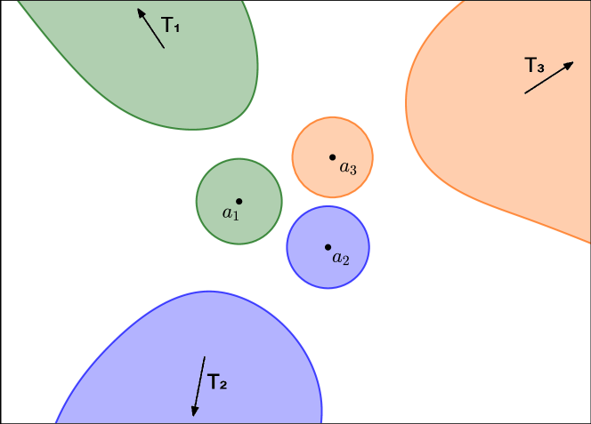
Figure 1. Sketch of a function with three transcendental singularities over its three distinct asymptotic values.

Now we proceed to define a dynamical version of $\mathbb{C}_{f}$ that we denote by $\mathbb{C}_{{f}^{{{\infty}}}}$. In addition to the asymptotic tracts of $f$, we also add for every asymptotic value $a\in S(f)$ the asymptotic tracts of every iterate of $f$ to the complex plane. Note that we might also need to identify tracts for different iterates of $f$, and we do so in the obvious way. More precisely, we set

$$\mathbb{C}_{{f}^{{{\infty}}}}:=\mathbb{C}\cup\left(\bigcup_{n\geq 1}\bigcup_{a\in S(f)}\bigcup_{\begin{subarray}{c}\text{eq. classes of asympt.}\\ \text{tracts of}f^{\circ n}\text{ over }a\end{subarray}}\{T\}\right)/\sim\;,$$

where $\sim$ denotes the equivalence relation that identifies tracts for different iterates of $f$. Our function $f$ extends to a continuous map $\widehat{f}\colon\mathbb{C}_{{f}^{{{\infty}}}}\to\mathbb{C}_{{f}^{{{\infty}}}}$.

Proposition 2.5 (Basic properties of the extension $\mathbb{C}_{{f}^{{{\infty}}}}$).

Let $f$ be an entire function for which the set $S(f)$ of singular values is finite. Then the extended map $\widehat{f}\colon\mathbb{C}_{{f}^{{{\infty}}}}\to\mathbb{C}_{{f}^{{{\infty}}}}$ is a covering over $\mathbb{C}_{{f}^{{{\infty}}}}\setminus S(f)$. If $g=f^{\circ n}$ is an iterate of $f$, we have $\mathbb{C}_{{f}^{{{\infty}}}}=\mathbb{C}_{{g}^{{{\infty}}}}$.

Proof.

The restriction $\left.f\right|_{\mathbb{C}\setminus f^{-1}(S(f))}$ is a covering map over $\mathbb{C}\setminus S(f)$ [GK86, Lemma 1.1]. It remains to show that every $T\in\mathbb{C}_{{f}^{{{\infty}}}}\setminus\mathbb{C}$ has a neighborhood $V$ such that $\widehat{f}|_{W}$ is a homeomorphism for every connected component $W$ of $\widehat{f}^{-1}(V)$.

Given a $T\in\mathbb{C}_{{f}^{{{\infty}}}}\setminus\mathbb{C}$, there exists a smallest $n\geq 1$ and an $a\in S(f)$ such that $\widehat{f}^{\circ n}(T)=a$. Choose $r>0$ such that $D_{r}(a)\cap P(f)=\{a\}$, and let $V$ be the component of $f^{-n}(D_{r}(a))$ in the tract represented by $T$. Let $V^{\prime}$ be a connected component of $f^{-1}(V)$, and let $T^{\prime}\in\mathbb{C}_{{f}^{{{\infty}}}}$ denote the tract represented by $V^{\prime}$. Then $h:=\left.f\right|_{V^{\prime}}\colon V^{\prime}\to V$ is biholomorphic because $V$ is simply connected and satisfies $V\cap P(f)=\emptyset$. The restriction extends to a homeomorphism

$$\widehat{h}\colon V^{\prime}\cup\{T^{\prime}\}\to V\cup\{T\}.$$

This shows that $\widehat{f}$ is a covering over $\mathbb{C}_{{f}^{{{\infty}}}}\setminus S(f)$.

To prove the second statement, just note that if $T$ is a tract of $f^{\circ n}$ over $a$, then $T$ is also a tract of $f^{\circ(n+m)}$ over $f^{\circ m}(a)$. ∎

There is a natural way to define the Julia set $\mathcal{J}(\widehat{f})$ and the Fatou set $\mathcal{F}(\widehat{f})$ of the extended map $\widehat{f}$: a point in $\mathbb{C}_{{f}^{{{\infty}}}}$ belongs to the Fatou resp. the Julia set if and only if the asymptotic value where the orbit first enters $\mathbb{C}$ belongs to the Fatou resp. Julia set of $f$. Finally, we define the set of critical points of $\widehat{f}$ as

$$C(\widehat{f}):=C(f)\cup(\mathbb{C}_{f}\setminus\mathbb{C})\;.$$

This is precisely the set of points that do not have a neighborhood on which $\widehat{f}$ is injective. In this sense, singular values of $f$ are critical values of $\widehat{f}$.

We will often discuss (pre-)periodic points; let us introduce the following notation.

Definition 2.6 ((Pre-)periodic points).

We denote by $\operatorname{PreP}(\widehat{f})\subset\mathbb{C}_{{f}^{{{\infty}}}}$ the set of points $p\in\mathbb{C}_{{f}^{{{\infty}}}}$ that are (pre-)periodic under iteration of $\widehat{f}$.

3. Dynamics of Post-Singularly Finite Entire Functions

3.1. Fatou Components and Internal Rays

Every periodic Fatou component, say $U$, is superattracting by Proposition 2.3. Therefore, $U$ contains a unique superattracting periodic point, called its center. The component comes with a Riemann map $\Phi\colon U\to\mathbb{D}$ that sends the center to $0$, and so that it conjugates the first return map on $U$ to $z\mapsto z^{d}$ on $\mathbb{D}$, for a unique $d\geq 2$ [Mil06, Theorems 9.1 and 9.3]; we call such a Riemann map a Böttcher map in analogy to the situation for polynomials. There are exactly $d-1$ choices for $\Phi$ [Mil06, Theorems 9.1]. An internal ray of $U$ is the preimage of a radial line in $\mathbb{D}$ under $\Phi$. For our purposes, an internal ray lands if its closure in the extended plane $\mathbb{C}_{{f}^{{{\infty}}}}$ intersects $\partial_{\mathbb{C}_{{f}^{{{\infty}}}}}U$ in a single point, and this single point is called the landing point of the ray.

It is well known that every periodic internal ray of a periodic Fatou component lands at a unique point $q\in\mathbb{C}$, and that $q$ is a repelling periodic point so that its period divides the period of the ray. (All this follows exactly as for polynomials, except one needs to show that the internal ray is bounded as a subset of $\mathbb{C}$; see [Rem08, Theorems B.1 and B.2]). Preperiodic internal rays of periodic Fatou components need not land in $\mathbb{C}$, but in any case they land at some point in $\mathbb{C}_{{f}^{{{\infty}}}}$. For example, the function $z\mapsto(z-1)\exp(z)+1$ has a fixed Fatou component containing a preperiodic ray that lands at a point at $\infty$.

Let us now extend centers and internal rays to a preperiodic Fatou component $V$. Let $n$ be minimal so that $U:=f^{\circ n}(V)$ is a periodic Fatou component. Then $f^{\circ n}\colon V\to U$ has finite or infinite mapping degree. In the case of finite mapping degree, it follows as for periodic Fatou components that $f^{\circ n}\colon V\to U$ can have only one critical point, and this point must map to the center of $U$. In this case, center and internal rays of $V$ can be defined naturally via pull-back, and all preperiodic internal rays must land in $\mathbb{C}$.

If $f^{\circ n}\colon V\to U$ has infinite mapping degree, similar reasons imply that as a subset of $\mathbb{C}$ it must factor through the exponential map as follows: there are Riemann maps $\psi\colon V\to\mathbb{H}\cup\{-\infty\}$ and $\phi\colon U\to\mathbb{D}$ so that $\phi$ maps the center of $U$ to $0$ (it is a Böttcher map) and $f^{\circ n}=\phi^{-1}\circ\widehat{\exp}\circ\psi\colon V\to U$, but here the additional point $-\infty\in\partial\mathbb{H}$ is part of the extended complex plane. In this case, the center of $V$ is at $\infty$. Internal rays in $U$ pull back to radial lines in $\mathbb{D}$ by $\phi$, then to horizontal lines in $\mathbb{H}$ by $\exp$, and finally give rise to uniquely defined internal rays in $V$. Every preperiodic internal ray in $V$ lands either at a repelling preperiodic point of $f$ in $\mathbb{C}$, or at a boundary point of $V$ in $\mathbb{C}_{{f}^{{{\infty}}}}\setminus\mathbb{C}$; both are preperiodic points in $\mathcal{J}(\widehat{f})$.

As we have just seen, every component $U$ of $\mathcal{F}(\widehat{f})$ has a well-defined and unique center $p$. We also denote the Fatou component with center $p$ by $U(p)$.

It is easy to see that for a given Fatou component distinct dynamic rays have distinct landing points.

Lemma 3.1 (Distinct landing points).

For any Fatou component of $\widehat{f}$, any two periodic or preperiodic internal rays land at distinct boundary points.

Proof.

It is sufficient to prove the statement for periodic Fatou components and periodic internal rays as the preperiodic case follows from pulling back periodic rays. Let $U$ be a periodic Fatou component. By passing to a suitable iterate, we may assume that $U$ as well as the internal rays $\beta_{1}$ and $\beta_{2}$ are fixed. By the Jordan curve theorem, there is a unique bounded component $V$ of $\mathbb{C}\setminus\overline{\beta_{1}\cup\beta_{2}}$. By the maximum modulus principle, we must have $f(V)\subset V$. On the other hand, as the dynamics of $f$ on $U$ is conjugated to $z\mapsto z^{d}$ on $\mathbb{D}$ (for some $d\geq 2$), it follows from the fact that $\beta_{1}$ and $\beta_{2}$ are fixed internal rays that $U\subset f(V)$ — a contradiction. ∎

3.2. The Escaping Set

One of the most important sets for studying the dynamics of entire functions is the set

$$I(f):=\{z\in\mathbb{C}\leavevmode\nobreak\ \colon\lim_{n\to\infty}f^{\circ n}(z)=\infty\}$$

of escaping points. The escaping set $I(f)$ is fully invariant and $I(f)\neq\emptyset$ [Ere89]. In many cases, and in particular for psf entire maps, the escaping set carries a rich combinatorial structure some aspects of which we are going to describe in the following.

In [RRRS11] it was shown that for a large class of transcendental entire maps the escaping set decomposes in a natural way into dynamic rays distinguished by external addresses so that the escaping dynamics of the map is semi-conjugate to the simple dynamics of the shift map on the space of external addresses. However, this class of maps does not include all post-singularly finite entire functions because components of the escaping set might have a more complicated topology than arcs, depending on the geometry of the tracts of the function [RRRS11]. Even in this more complicated case, the escaping set still decomposes in a natural way into unbounded connected components called dreadlocks [BRG20]. These dreadlocks share many similarities with rays: their connected components are again distinguished by external addresses so that the escaping dynamics is semi-conjugate to the dynamics of the shift map, and thus they can be viewed as natural generalizations of dynamic rays. In the following, we describe the natural decomposition of the escaping set into dreadlocks and their combinatorial description via external addresses.

The construction we describe below can be carried out more generally for functions with bounded post-singular set [BRG20], but in this paper we focus on post-singularly finite functions $f$. Let $D\supset P(f)$ be an open disk centered at the origin. The connected components of $f^{-1}(\mathbb{C}\setminus\overline{D})$ are called tracts of $f$ over $\infty$. It is easy to see that every tract $T$ of $f$ is simply connected, unbounded, that $\partial T$ is a Jordan arc tending to infinity in both directions, and that the restriction $\left.f\right|_{T}$ is a universal covering over $\mathbb{C}\setminus\overline{D}$. Let $\alpha:[0,1)\to\mathbb{C}$ be an arc connecting $\partial D$ to $\infty$ that satisfies $\alpha\cap D=\emptyset$ and $\alpha\cap f^{-1}(\mathbb{C}\setminus\overline{D})=\emptyset$; see Figure 2.

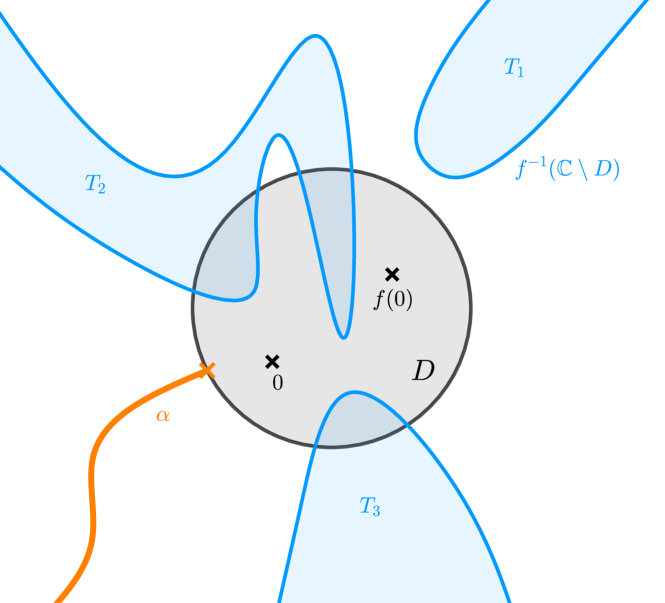
Figure 2. A sketch of a possible configuration of $D$ and $\alpha$.

We set $W_{0}:=\mathbb{C}\setminus(\overline{D}\cup\alpha)$. The domain $W_{0}$ is simply connected with $P(f)\cap W_{0}=\emptyset$. Therefore, for every $n\geq 0$, every component of $f^{-n}(W_{0})$ maps biholomorphically onto $W_{0}$; see Figure 3.

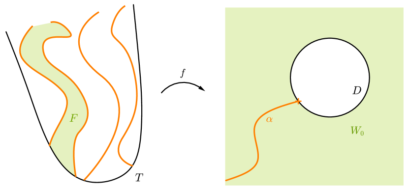
Figure 3. Sketch of $W_{0}$ and a fundamental domain $F$.

Definition 3.2 (Fundamental tails and external addresses).

A connected component $\tau$ of $f^{-n}(W_{0})$ is called a fundamental tail of level $n$. A fundamental tail of level $1$ is called a fundamental domain and is commonly denoted as $F$. We denote the set of all fundamental domains by $\mathscr{S}(D,\alpha)$ and call it a static partition for $f$.

An external address $\underline{s}:=(F_{i})_{i=0}^{\infty}=F_{0}F_{1}\ldots$ is a sequence of fundamental domains $F_{i}$. We denote the space of external addresses of all external addresses by $\mathbf{S}$ and define the shift map

$$\sigma\colon\mathbf{S}\to\mathbf{S},\leavevmode\nobreak\ \sigma(F_{0}F_{1}F_{2}\ldots)=F_{1}F_{2}\ldots\leavevmode\nobreak\ \leavevmode\nobreak\ \leavevmode\nobreak\ \text{for all}\leavevmode\nobreak\ \underline{s}=(F_{i})_{i=0}^{\infty}\in\mathbf{S}.$$

We call the external address $\underline{s}$ bounded if it contains only finitely many distinct $F_{i}$. The address $\underline{s}$ is called periodic if it is periodic under iteration of $\sigma$, and preperiodic if it is preperiodic under iteration of $\sigma$.

Let $\tau$ be a fundamental tail of level $n>1$. Then $\tau$ is a Jordan domain on $\hat{\mathbb{C}}$ containing $\infty$ on its boundary, and we have $f^{\circ k}(z)\to\infty$ as $z\to\infty$ in $\tau$ for all $k\leq n$. It follows that $\tau$ tends to infinity through some fundamental domain. More precisely, there exists a unique fundamental domain $F$ such that $\overline{\tau}\setminus F$ is bounded, see [BRG20, Lemma 3.6]. Therefore, we can naturally associate a finite external address to each fundamental tail, see [BRG20, Definition 3.7].

Definition 3.3 (Addresses of fundamental tails).

Let $\tau$ be a fundamental tail of level $n$, and denote for $k<n$ by $F_{k}(\tau)$ the unique fundamental domain whose intersection with the fundamental tail $f^{\circ k}(\tau)$ is unbounded. We call the finite sequence $\underline{s}=F_{0}(\tau)F_{1}(\tau)\ldots F_{n-1}(\tau)$ the (finite) external address of $\tau$.

Every finite external address is realized by one and only one fundamental tail, see [BRG20, Definition and Lemma 3.8].

Lemma and Definition 3.4 (Tails at a given address).

Let $\underline{s}=F_{0}F_{1}\ldots$ be a finite or infinite sequence of fundamental domains that has length at least $n\geq 1$. Then there exists a unique fundamental tail $\tau$ of level $n$ that has address $\tilde{\underline{s}}:=F_{0}F_{1}\ldots F_{n-1}$. We denote this fundamental tail by $\tau_{n}(\underline{s})$; see Figure 4 for a visualization. We also define the inverse branches

$$f_{\underline{s}}^{-n}:=(\left.f^{\circ n}\right|_{\tau_{n}(\underline{s})})^{-1}\colon W_{0}\to\tau_{n}(\underline{s}).$$

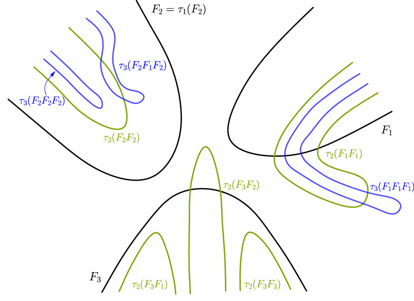
Figure 4. Sketch of some fundamental tails of various levels. For a given address $\underline{s}$, the fundamental tails $\tau_{n}(\underline{s})$ might be nested or not. Fundamental tails of different levels might intersect, even if one is not the prefix of the other.

Let us collect some more results about fundamental tails from [BRG20, Observation 3.9] that follow more or less directly from the preceding results and definitions.

Lemma 3.5 (Further facts about fundamental tails).

Let $\tau$ be a fundamental tail of level $n$ and let $\underline{s}$ be the address of $\tau$. Then the address of $f(\tau)$ is $\sigma(\underline{s})$.

Suppose that $\tau^{1}$ and $\tau^{2}$ are fundamental tails of levels $n_{1}$ and $n_{2}$ with $n_{1}\geq n_{2}$. Let $\underline{s}^{1}$ and $\underline{s}^{2}$ be the addresses of $\tau^{1}$ and $\tau^{2}$ respectively. Then $\tau^{1}\cap\tau^{2}$ is unbounded if and only if $\underline{s}^{1}$ is a prefix of $\underline{s}^{2}$, i.e., $\underline{s}^{2}=\underline{s}^{1}F_{n_{1}}\ldots F_{n_{2}-1}$. In this case, if additionally $n_{1}>n_{2}$, all sufficiently large points of $\overline{\tau^{1}}$ are contained in $\tau^{2}$.

In order to define dreadlocks, we introduce the unbounded component of fundamental tails.

Definition 3.6 (Unbounded component of fundamental tails).

Let $F$ be a fundamental domain. We denote by $\accentset{\infty}{F}$ the unique unbounded connected component of $F\setminus\overline{D}$; see Figure 5.

More generally, let $\tau$ be a fundamental tail of level $n$. We define $\accentset{\infty}{\tau}$ to be the unbounded connected component of $\tau\setminus f^{-(n-1)}(\overline{D})$. In other words, if $F=f^{\circ(n-1)}(\tau)$, then $\accentset{\infty}{\tau}$ is the component of $f^{-(n-1)}(\accentset{\infty}{F})$ contained in $\tau$.

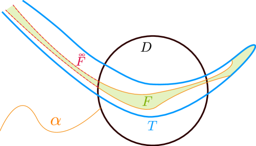
Figure 5. Sketch of the unbounded component of a fundamental domain $F$.

Note that $\accentset{\infty}{\tau}_{n}(\underline{s})$ is the unbounded connected component of $\tau_{n}(\underline{s})\cap\tau_{n-1}(\underline{s})$ for $n\geq 2$. We have finally gathered the necessary terminology to formally define dreadlocks.

Definition 3.7 (Dreadlocks).

Let $\underline{s}$ be an external address. We say that a point $z\in\mathbb{C}$ has external address $\underline{s}$ if $z\in\accentset{\infty}{\tau}_{n}(\underline{s})$ for all sufficiently large $n$.

The dreadlock $G_{\underline{s}}$ is defined to be the set of points $z\in\mathbb{C}$ that have external address $\underline{s}$ and are contained in $I(f)$.

It follows directly from Definition 3.6 and Definition 3.7 that every escaping point has an external address. Therefore, every escaping point is contained in one and only one dreadlock.

While dreadlocks provide a decomposition of the escaping set, they depend a priori on the choice of the base domain $W_{0}$. However, it turns out that the decomposition of the escaping set into dreadlocks is independent of the choice of the base domain, and external addresses w.r.t. any two given base domains are in natural bijection to each other, see [BRG20, p.24 and Observation 4.12] for an explanation.

Another important fact is that a function has the same dreadlocks as any of its iterates; moreover, external addresses for the function are in natural bijection to external addresses for its iterate, see [BRG20, p.25 and Observation 4.13].

Lemma 3.8 (Dreadlocks of iterates).

Let $f$ be a psf entire function, and let $n\geq 1$. Then every dreadlock of $f$ is a dreadlock of $f^{\circ n}$ and vice versa.

We summarize the results obtained on the escaping dynamics of psf entire functions in one theorem below, see [BRG20, Lemma 4.3, Corollary 4.5, and Proposition 4.10].

Theorem 3.9 (The escaping set of a post-singularly finite entire function).

Let $f$ be a post-singularly finite entire function. The escaping set $I(f)=\mathop{\vphantom{\bigcup}\mathchoice{\leavevmode\vtop{\halign{\hfil$\m@th\displaystyle#$\hfil\cr\bigcup\cr\cdot\crcr}}}{\leavevmode\vtop{\halign{\hfil$\m@th\textstyle#$\hfil\cr\bigcup\cr\cdot\crcr}}}{\leavevmode\vtop{\halign{\hfil$\m@th\scriptstyle#$\hfil\cr\bigcup\cr\cdot\crcr}}}{\leavevmode\vtop{\halign{\hfil$\m@th\scriptscriptstyle#$\hfil\cr\bigcup\cr\cdot\crcr}}}}\displaylimits_{\underline{s}\in\mathbf{S}}G_{\underline{s}}$ decomposes in a natural way into subsets indexed by external addresses called dreadlocks. For every $\underline{s}\in\mathbf{S}$, either $G_{\underline{s}}=\emptyset$ or $G_{\underline{s}}$ is unbounded and connected. We have $f(G_{\underline{s}})=G_{\sigma(\underline{s})}$.

Not every external address is actually realized by points in $\mathbb{C}$: the growth of $f$ imposes a limit on the growth of realized external addresses [SZ03a]. However, every bounded address is realized, and especially every (pre-)periodic address. The latter are the ones we are interested in here.

3.2.1. Cyclic Order of Dreadlocks.

We denote a cyclic order on a set $X$ by $a\prec b\prec c$, where $a,b,c\in X$. For convenience, we write

$$a_{1}\prec a_{2}\prec\ldots\prec a_{n},$$

where we use $\prec$ to stress that this is a cyclic order of $n\geq 3$ elements $a_{j}\in X$, not a linear order. This expression means that $a_{j-1}\prec a_{j}\prec a_{j+1}$ for all $j\in\{1,\ldots,n\}$, where indices are labeled mod $n$. Expressions such as

$$a\preceq b\prec c$$

mean that either $a\prec b\prec c$ or $a=b\prec c$.

There is a natural cyclic order on the set of fundamental domains. Given three fundamental domains $F_{0}$, $F_{1}$, and $F_{2}$, we choose, for $i\in\{0,1,2\}$, arcs $\gamma_{i}\colon[0,1]\to\hat{\mathbb{C}}$ connecting some point $\zeta_{i}=\gamma_{i}(0)\in F_{i}$ to $\infty=\gamma_{i}(1)$ and satisfying $\gamma_{i}((0,1))\subset F_{i}$. Let $R>0$ be large enough such that each of the arcs $\gamma_{i}$ contains a point of modulus $R$, and set $t_{i}:=\max_{t\in[0,1]}\{t\colon|\gamma_{i}(t)|=R\}$. The points $\gamma_{i}(t_{i})$ have a counter-clockwise cyclic order on the circle $\partial D_{R}(0)$, and this is by definition the cyclic order of the arcs $\gamma_{i}$ at infinity. It is not hard to see that this cyclic order is well defined, i.e. independent of the choice of $R$. Indeed, if the cyclic order were different for $\tilde{R}\neq R$, the arcs $\gamma_{i}$ would not be pairwise disjoint.

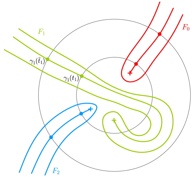
Figure 6. Sketch of the arcs $\gamma_{i}$ used to defined the cyclic order of the fundamental domains $F_{i}$. The arc $\gamma_{1}$ shows that it is important to use the maximal potential $t_{i}$ at which $\gamma_{i}$ intersects $D_{R}(0)$.

The cyclic order of the fundamental domains $F_{i}$ is, by definition, the same as the cyclic order of the corresponding curves $\gamma_{i}$. This order is well-defined, i.e., independent of the choice of the $\gamma_{i}$, because every fundamental domain has a unique access to $\infty$.

Even though there are countably many fundamental domains, the cyclic order is such that each of them has a unique predecessor and successor. We describe this as follows.

Lemma and Definition 3.10 (Successors of fundamental domains).

Let $\mathscr{S}(D,\alpha)$ be a static partition, and let $F\in\mathscr{S}(D,\alpha)$ be a fundamental domain. Then there are unique fundamental domains $F_{p},F_{s}\in\mathscr{S}(D,\alpha)$, called the predecessor and successor of $F$, such that every $F^{\prime}\in\mathscr{S}(D,\alpha)\setminus\{F_{p},F,F_{s}\}$ satisfies

$$F^{\prime}\prec F_{p}\prec F\prec F_{s}\;.$$

Proof.

This follows directly from the topology of fundamental domains. ∎

For a given $N\geq 1$, the fundamental tails of level $N$ are also pairwise disjoint Jordan domains on $\hat{\mathbb{C}},$ each with a unique access to $\infty$. Therefore, the same construction as above allows us to define a cyclic order on the set of fundamental tails of level $N$ for any given $N\geq 1$. These orders can be used to define a cyclic order on the space of external addresses.

Definition 3.11 (Cyclic order of external addresses).

Let $\underline{s}$, $\underline{t}$, and $\underline{u}$ be distinct external addresses. Choose $N\geq 1$ large enough so that the fundamental tails $\tau_{N}(\underline{s})$, $\tau_{N}(\underline{t})$, and $\tau_{N}(\underline{u})$ of level $N$ are distinct. Define the cyclic order of the addresses via

$$\underline{s}\prec\underline{t}\prec\underline{u}:\Leftrightarrow\tau_{N}(\underline{s})\prec\tau_{N}(\underline{t})\prec\tau_{N}(\underline{u}).$$

By Lemma 3.5, all points of $\tau_{M}(\underline{s})$ with sufficiently large absolute values are contained in $\tau_{N}(\underline{s})$ for each $M\geq N$. Therefore, the cyclic order on $\mathbf{S}$ is well defined. It induces a topology on the space of external addresses (this works on the level of all external addresses, whether or not they are realized).

Definition 3.12 (Order topology on $\mathbf{S}$).

For distinct external addresses $\underline{s},\underline{t}$ we define intervals between $\underline{s},\underline{t}$ as

$$(\underline{s},\underline{t}):=\{\underline{u}\in\mathbf{S}\colon\underline{s}\prec\underline{u}\prec\underline{t}\},$$

$$(\underline{s},\underline{t}]:=\{\underline{u}\in\mathbf{S}\colon\underline{s}\prec\underline{u}\preceq\underline{t}\},$$

$$[\underline{s},\underline{t}):=\{\underline{u}\in\mathbf{S}\colon\underline{s}\preceq\underline{u}\prec\underline{t}\},$$

$$[\underline{s},\underline{t}]:=\{\underline{u}\in\mathbf{S}\colon\underline{s}\preceq\underline{u}\preceq\underline{t}\}.$$

The open intervals form $(\underline{s},\underline{t})$ the basis of the order topology on $\mathbf{S}$.

When we do topological constructions in $\mathbf{S}$ (as e.g. in Proposition 8.8), the underlying topology is always the order topology. As dreadlocks are parametrized by external addresses, the cyclic order on the space of external addresses can be used to define a cyclic order on the set of dreadlocks.

Definition 3.13 (Cyclic order of dreadlocks).

We define a cyclic order on the set of dreadlocks via

$$G_{\underline{s}}\prec G_{\underline{t}}\prec G_{\underline{u}}:\Leftrightarrow\underline{s}\prec\underline{t}\prec\underline{u}$$

for distinct dreadlocks $G_{\underline{s}}$, $G_{\underline{t}}$, and $G_{\underline{u}}$.

In [BRG20, Sections 4 and 12], an equivalent but more direct definition of the cyclic order of dreadlocks at infinity that does not need external addresses is given.

3.2.2. Intermediate Addresses and Linear Order.

Let $f\in\mathcal{B}$ be of bounded type, and let $\mathscr{S}(D,\alpha)$ be a static partition for $f$. In [BJR12, Section 5], a dynamical compactification of the complex plane (depending on $f$ and $\mathscr{S}(D,\alpha)$) was obtained by adding a circle of addresses at infinity. The authors defined an extension $\overline{\mathbf{S}}\supset\mathbf{S}$, where $\overline{\mathbf{S}}$ is the completion of $\mathbf{S}$ w.r.t. the cyclic order. The elements of $\overline{\mathbf{S}}\setminus\mathbf{S}$ are called intermediate addresses, and the extension $\overline{\mathbf{S}}$ is called the circle of addresses. The dynamical compactification is then defined to be $\mathbb{C}_{\overline{\mathbf{S}}}:=\mathbb{C}\mathbin{\mathchoice{\leavevmode\vtop{\halign{\hfil$\m@th\displaystyle#$\hfil\cr\cup\cr\cdot\crcr}}}{\leavevmode\vtop{\halign{\hfil$\m@th\textstyle#$\hfil\cr\cup\cr\cdot\crcr}}}{\leavevmode\vtop{\halign{\hfil$\m@th\scriptstyle#$\hfil\cr\cup\cr\cdot\crcr}}}{\leavevmode\vtop{\halign{\hfil$\m@th\scriptscriptstyle#$\hfil\cr\cup\cr\cdot\crcr}}}}\overline{\mathbf{S}}$ equipped with a suitable topology. In this topology, $\overline{\mathbf{S}}$ is homeomorphic to the unit circle and $\mathbb{C}_{\overline{\mathbf{S}}}$ is homeomorphic to the closed unit disk. The details of this constructions are described in [BJR12, Section 5]; here, we will just describe a few special cases that we need, associated to the curve $\alpha$ and its immediate preimages.

Given distinct external addresses $\underline{s}\neq\underline{t}\in\mathbf{S}$, we choose $N\geq 1$ large enough such that the fundamental tails $\tau_{N}(\underline{s})$ and $\tau_{N}(\underline{t})$ of level $N$ are disjoint. Choose arcs $\gamma_{\underline{s}}\colon[0,1]\to\tau_{N}(\underline{s})\cup\{\infty\}$ and $\gamma_{\underline{t}}\colon[0,1]\to\tau_{N}(\underline{t})\cup\{\infty\}$ connecting arbitrary base points to $\infty$. Since $\alpha$ does not intersect the tracts of $f$, some unbounded part $\alpha^{\prime}$ of $\alpha$ satisfies $\alpha^{\prime}\cap\tau_{N}^{i}=\emptyset$ ($i\in\{1,2\}$). Hence, the arcs $\gamma_{\underline{s}}$, $\gamma_{\underline{t}}$, and $\alpha^{\prime}$ are pairwise disjoint and have a well-defined cyclic order at infinity. We define

$$\alpha\prec\underline{s}\prec\underline{t}:\Leftrightarrow\alpha^{\prime}\prec\gamma_{\underline{s}}\prec\gamma_{\underline{t}}.$$

It follows as before that this cyclic order is well-defined. We define $\alpha\in\overline{\mathbf{S}}\setminus\mathbf{S}$ to be an intermediate address (the ambiguous usage of $\alpha$ should not cause any confusion).

Now consider any immediate preimage $\tilde{\alpha}$ of $\alpha$. There is a unique fundamental domain $F\in\mathscr{(}D,\alpha)$ such that $\tilde{\alpha}\subset\partial F_{p}\cap\partial F$ (see Definition 3.10: $\tilde{\alpha}$ is between $F$ and its predecessor). We denote this lift by $\alpha_{F_{p}}^{F}\in\overline{\mathbf{S}}\setminus\mathbf{S}$. Analogously to the case of $\alpha$, we can extend the cyclic order to all $\alpha_{F_{p}}^{F}$.

There are many more intermediate addresses, but we will not need them here.

Finally, note that every cyclic order can be turned into a linear order by removing an arbitrary element. We do this with respect to the distinguished intermediate address $\alpha\in\overline{\mathbf{S}}\setminus\mathbf{S}$ (the simplest intermediate address).

Definition 3.14 (Linear and cyclic order of external addresses).

Let $\underline{s}=F_{0}F_{1}\ldots$ and $\underline{t}=F_{0}^{\prime}F_{1}^{\prime}$ be distinct external addresses. We define a linear order on $\mathbf{S}$ via

$$\underline{s}<\underline{t}:\Leftrightarrow\alpha\prec\underline{s}\prec\underline{t}.$$

4. Landing of Dreadlocks

Our main focus in this paper are (pre-)periodic dreadlocks and their landing behavior. If the dreadlock $G_{\underline{s}}$ happens to be a dynamic ray, i.e., if it can be parametrized via a homeomorphism $\gamma\colon(0,\infty)\to G_{\underline{s}}$ satisfying $\lim_{t\to+\infty}\gamma(t)=\infty$, then it is clear how to define the accumulation set $\Lambda(G_{\underline{s}})$ of $G_{\underline{s}}$: we just set

$$\Lambda(G_{\underline{s}}):=\bigcap_{t>0}\overline{\gamma((0,t))}.$$

In general, the topology of $G_{\underline{s}}$ is more complicated, so we need a more abstract way to define the accumulation set of a dreadlock. An additional problem comes from the fact that there might be preperiodic dreadlocks that do not accumulate anywhere in $\mathbb{C}$ but that do land, in a meaningful way, in the extended plane $\mathbb{C}_{{f}^{{{\infty}}}}$. Indeed, this happens if and only if $f$ has asymptotic values, so it happens even for preperiodic dynamic rays of psf exponential maps; see Figure 7 for an example.

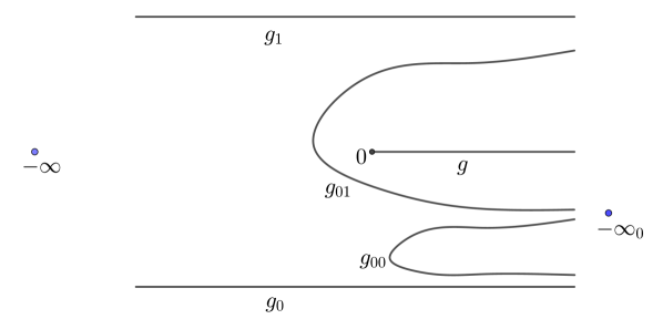
Figure 7. For every psf exponential map $\lambda\mapsto\lambda\exp(z)$, there exists a preperiodic dynamic ray $g$ that lands at $0$ [SZ03b]. The preimage rays $g_{0}$ and $g_{1}$ of $g$ do not land anywhere in $\mathbb{C}$, but they land at $-\infty\in\mathbb{C}_{\lambda\exp}$. The preimages $g_{01}$ of $g_{1}$ and $g_{00}$ of $g_{0}$ land together at a preimage $-\infty_{0}\in\mathbb{C}_{{\lambda\exp}^{{{\infty}}}}$ of $-\infty$.

In [BRG20, Definition 6.1], a definition for the accumulation set in $\hat{\mathbb{C}}$ of a dreadlock at an arbitrary bounded external address was given. We adapt that definition to our extension of $\mathbb{C}$. Recall the choice of inverse branches $f_{\underline{s}}^{-n}(\zeta)\in\tau_{n}(\underline{s})$ from Lemma and Definition 3.4, as well as domain $W_{0}:=\mathbb{C}\setminus(\overline{D}\cup\alpha)$ from the beginning of Section 3.2.

Definition 4.1 (Accumulation sets of dreadlocks).

For a bounded external address $\underline{s}$, we define the accumulation set in $\mathbb{C}_{{f}^{{{\infty}}}}$ of the dreadlock $G_{\underline{s}}$ as the set of all possible limit points in $\mathbb{C}_{{f}^{{{\infty}}}}$ of sequences $(\zeta_{n})_{n=1}^{\infty}$ defined by taking an arbitrary base point $\zeta\in W_{0}$ and, for $n\geq 1$, setting $\zeta_{n}:=\zeta_{n}(\underline{s}):=f_{\underline{s}}^{-n}(\zeta)\in\tau_{n}(\underline{s})$. We denote this accumulation set as

$$\Lambda_{\mathbb{C}_{{f}^{{{\infty}}}}}(G_{\underline{s}}):=\Lambda_{\mathbb{C}_{{f}^{{{\infty}}}}}(\underline{s})\;.$$

We say that the dreadlock $G_{\underline{s}}$ lands at a point $p\in\mathbb{C}_{{f}^{{{\infty}}}}$ if and only if $\Lambda_{\mathbb{C}_{{f}^{{{\infty}}}}}(\underline{s})=\{p\}$. In this case, we also denote the landing point of $G_{\underline{s}}$ by $L(\underline{s})\in\mathbb{C}_{{f}^{{{\infty}}}}$.

The main result of [BRG20] is a generalization of the Douady–Hubbard landing theorem for post-singularly bounded polynomials to post-singularly bounded entire functions. We state a restricted version of [BRG20, Theorem 7.1] for post-singularly finite entire functions.

Theorem 4.2 (Landing theorem for dreadlocks).

Let $f$ be a psf entire function. Then every periodic dreadlock of $f$ lands at a repelling periodic point $p\in\mathcal{J}(f)$.

Conversely, every periodic point $p\in\mathcal{J}(f)$ is the landing point of at least one and at most finitely many dreadlocks, all of which are periodic of the same period.

A point $p\in\mathbb{C}_{{f}^{{{\infty}}}}\setminus\mathbb{C}$ cannot be periodic because it is eventually mapped to a periodic post-singular value in $\mathbb{C}$ and is not part of its periodic orbit, so Theorem 4.2 only makes a statement about points in $\mathbb{C}$ and dreadlocks landing in $\mathbb{C}$. Using the extended plane $\mathbb{C}_{{f}^{{{\infty}}}}$, Theorem 4.2 extends neatly to the case of preperiodic dreadlocks.

Lemma 4.3 (Landing of (pre-)periodic dreadlocks in $\mathbb{C}_{{f}^{{{\infty}}}}$).

Let $f$ be a psf entire function. Then every (pre-)periodic dreadlock of $f$ lands at a repelling (pre-)periodic point $p\in\mathcal{J}(\widehat{f})$.

Conversely, every (pre-)periodic point $p\in\mathcal{J}(\widehat{f})$ is the landing point of at least one and possibly infinitely many (pre-)periodic dreadlocks, all of which have the same period and preperiod.

In contrast to the periodic case, there might be preperiodic points at which infinitely many dreadlocks land together. This does not happen for preperiodic points in $\mathbb{C}$, but does happen precisely for all $p\in\mathcal{J}(\widehat{f})\setminus\mathcal{J}(f)$ (the point $-\infty$ in Figure 7 is an example of such a point). The proof of Lemma 4.3 is given at the end of Section 5 because we need to establish some topological properties of dreadlocks beforehand. We are now ready to define the main object of this paper.

Definition 4.4 (Landing equivalence).

We write $\mathbf{S}^{\operatorname{PreP}}$ for the set of (pre-)periodic external addresses. Given two addresses $\underline{s},\underline{t}\in\mathbf{S}^{\operatorname{PreP}}$, we write $\underline{s}\sim_{\operatorname{land}}\underline{t}$ if the dreadlocks $G_{\underline{s}}$ and $G_{\underline{t}}$ land together in $\mathbb{C}_{{f}^{{{\infty}}}}$, i.e., if $L(\underline{s})=L(\underline{t})$. We call the equivalence relation $\sim_{\operatorname{land}}$ on $\mathbf{S}^{\operatorname{PreP}}$ the landing equivalence relation.

Our main result is that for all psf entire functions and all (pre-)periodic dreadlocks the landing equivalence relation can be described in terms of itineraries of dreadlocks with respect to a dynamically meaningful partition of the plane. Roughly speaking, two periodic dreadlocks land together if and only if they have the same itinerary with respect to this partition; for preperiodic dreadlocks, the situation is a bit more complicated because preperiodic dreadlocks might share a landing point that lies on the boundary of several partition sectors. The conceptual idea is not new, and so-called dynamic partitions have been defined in many other contexts in complex dynamics: for post-critically finite polynomials, one picks for every critical value an (extended) dynamic ray that lands at this value. The preimages of these (extended) rays naturally divide the complex plane into partition sectors, and periodic points can be distinguished in terms of their itineraries, see [Poi09]. In [SZ03b], dynamic partitions were defined for certain classes of exponential maps (attracting, parabolic, escaping, and psf parameters), and this is also where the term “dynamic partition” was introduced. In [MB09], dynamic partitions were defined for geometrically finite entire maps with dynamic rays. While many arguments given in this paper work in analogy to previous work on dynamic partitions, additional complications come from the fact that we are dealing with dreadlocks instead of dynamic rays, and from having to deal with preperiodic dreadlocks that do not land in $\mathbb{C}$ but in our extension of $\mathbb{C}$. We need to show some facts about the topology of dreadlocks before we can define and use dynamic partitions in the general case.

5. Topology of Dreadlocks

In this section, we establish some topological results regarding dreadlocks. We construct certain simply connected enclosing domains for dreadlocks that are easier to deal with than dreadlocks from the point of view of covering space theory and help us proof Lemma 4.3. Moreover, we discuss separation properties of dreadlocks, especially when several land at a common point. Finally, we introduce the concept of extended dreadlocks that helps us deal with post-singular points in the Fatou set.

5.1. Enclosing Domains

We start by showing that for $n$ large enough only those points of $G_{\underline{s}}$ very close to the landing point $p$ are not contained in $\accentset{\infty}{\tau}_{n}(\underline{s})$. For the proof, we need the following result [BRG20, Proposition 4.4].

Proposition 5.1.

Let $\underline{s}=(F_{n})_{n=0}^{\infty}$ be an external address. If $z\in I(f)$ satisfies $f^{\circ n}(z)\in\accentset{\infty}{F}_{n}$ for all $n\geq 0$, then $z\in G_{\underline{s}}$. Moreover, we have $z\in\accentset{\infty}{\tau}_{n}(\underline{s})$ for all $n\geq 1$.

Lemma 5.2 (Enclosing domains).

Assume that the (pre-)periodic dreadlock $G_{\underline{s}}$ lands at a point $p\in\mathbb{C}$. Then for every $\varepsilon>0$ there exists an $N\geq 1$ such that for all $n\geq N$ we have

$$\overline{G_{\underline{s}}}\subset D_{\varepsilon}(p)\cup\accentset{\infty}{\tau}_{n}(\underline{s}).$$

Proof.

We write $\underline{s}=(F_{n})_{n=0}^{\infty}$. By [BRG20, Proposition 6.5(f)], on $\tilde{G}:=G_{\underline{s}}\setminus D_{\varepsilon}(p)$ iteration of $f$ tends to infinity uniformly. Therefore, there exists an $N\geq 1$ such that for every $z\in\tilde{G}$ we have $f^{\circ n}(\tilde{G})\subset\accentset{\infty}{F}_{n}(z)$ for all $n\geq N$ and certain fundamental domains $F_{n}(z)$. As $f^{\circ N}(\tilde{G})\subset G_{\sigma^{\circ N}(\underline{s})}$, Proposition 5.1 implies that the $F_{n}(z)$ are independent of $z\in\tilde{G}$ and satisfy $F_{n}(z)=F_{n}$. The second part of Proposition 5.1 implies that $f^{\circ N}(\tilde{G})\subset\accentset{\infty}{\tau}_{n}(\sigma^{\circ N}(\underline{s}))$ for all $n\geq 1$. It follows by pulling back $N$ times that $\tilde{G}\subset\accentset{\infty}{\tau}_{n}(\underline{s})$ for all $n\geq N+1$. ∎

For the construction of the nested enclosing domains, we need two additional results. The first one is a lemma on the shrinking of preimage domains [BRG20, Lemma 6.2].

Lemma 5.3 (Euclidean shrinking).

Suppose that $\Omega\subset\mathbb{C}\setminus P(f)$ is a bounded Jordan domain. Then, for every $\varepsilon>0$ and every compact set $K\subset\mathbb{C}$, there exists $N_{\varepsilon}$ with the following property: for every $n\geq N_{\varepsilon}$, every connected component of $f^{-n}(\Omega)$ that intersects $K$ has Euclidean diameter at most $\varepsilon$.

It was shown in [BRG20, Theorem 7.1] that a single dreadlock that lands in $\mathbb{C}$ does not separate $\mathbb{C}$.

Proposition 5.4 (Topology of landing dreadlocks).

If $G_{\underline{s}}$ is a (pre-)periodic dreadlock that lands in $\mathbb{C}$, then $\operatorname{cl}(G_{\underline{s}})$ does not separate $\mathbb{C}$.

Lemma 5.5 (Nested enclosing domains).

Let $G_{\underline{s}}$ be a (pre-)periodic dreadlock that lands at some point $p\in\mathbb{C}$. Then there exists a nested sequence of simply connected domains $U_{n}\subset\mathbb{C}$ ($n\geq 1$) such that

$$\bigcap_{n}U_{n}=\bigcap_{n}\overline{U_{n}}=\overline{G_{\underline{s}}}.$$

Moreover, we have $\overline{U_{n+1}}\subset U_{n}$ for all $n$ and $\tau_{m}(\underline{s})\subset U_{n}$ for all $m\geq n$.

Proof.

We choose for every of the finitely many fundamental domains $F$ occurring in $\underline{s}=(F_{n})_{n=0}^{\infty}$ a bounded Jordan domain $\Omega_{F}\subset\mathbb{C}\setminus P(f)$ such that $\Omega_{F}\cap F\neq\emptyset$ and $\tilde{F}:=F\setminus\overline{\Omega_{F}}$ satisfies $\operatorname{cl}(\tilde{F})\subset W_{0}$. Furthermore, we define $\tilde{\tau}_{n}(\underline{s})\subset\accentset{\infty}{\tau}_{n}(\underline{s})$ to be the unique preimage component of $\tilde{F}_{n-1}$ under $f^{\circ(n-1)}$ contained in $\accentset{\infty}{\tau}_{n}(\underline{s})$. It follows that

$$\operatorname{cl}(\tilde{\tau}_{n}(\underline{s}))\subset\tau_{n-1}(\underline{s})$$ (1)

It follows from Lemma 5.3 that for every $\varepsilon>0$ there exists an $N\in\mathbb{N}$ such that $\tau_{n}(\underline{s})\setminus\tilde{\tau}_{n}(\underline{s})\subset D_{\varepsilon}(p)$ for all $n\geq N$. Using this fact and Lemma 5.2, we are able to construct a sequence $\varepsilon_{n}\searrow 0$ such that ${\overline{G_{\underline{s}}}\subset D_{\varepsilon_{n}}(p)\cup\tau_{n}(\underline{s})}=:V_{n}$ and $\tau_{n}(\underline{s})\setminus\tilde{\tau}_{n}(\underline{s})\subset D_{\varepsilon_{n}}(p)$. In particular, we have

$$V_{n}=D_{\varepsilon_{n}}(p)\cup\tau_{n}(\underline{s})=D_{\varepsilon_{n}}(p)\cup\tilde{\tau}_{n}(\underline{s}).$$

Using (1), we conclude that

$$\overline{V_{n+1}}=\operatorname{cl}(D_{\varepsilon_{n+1}}(p))\cup\operatorname{cl}(\tilde{\tau}_{n+1}(\underline{s}))\subset D_{\varepsilon_{n}}(p)\cup\tau_{n}(\underline{s})=V_{n}.$$

Given a $z\in\bigcap_{n}V_{n}\setminus\{p\}$, it follows that $z\in\accentset{\infty}{\tau}_{n}(\underline{s})$ for all sufficiently large $n$. But this means, by definition, that $z$ has external address $\underline{s}$, hence $z\in G_{\underline{s}}$. This shows $\overline{G_{\underline{s}}}=\bigcap_{n}V_{n}$. We have $\tau_{m}(\underline{s})\subset V_{n}$ for $m\geq n$ by construction.

Every $V_{n}$ has a unique unbounded complementary component $C_{n}\subset\mathbb{C}\setminus V_{n}$. We set $U_{n}:=\mathbb{C}\setminus C_{n}$. Then $U_{n}\subset V_{n}$ is simply connected and we have $\overline{U_{n+1}}\subset U_{n}$. Given a point $z\in\mathbb{C}\setminus\overline{G_{\underline{s}}}$, we connect $z$ to a point $w\in C_{1}$ via an arc $\gamma$ that satisfies $\gamma\cap\overline{G_{\underline{s}}}=\emptyset$. This is possible by Proposition 5.4. Then $\gamma$ has some positive spherical distance from $\overline{G_{\underline{s}}}$, so there exists an $N$ such that for $n\geq N$ we have $\gamma\cap\overline{V_{n}}=\emptyset$. This means $z\in C_{n}=\mathbb{C}\setminus U_{n}$. We conclude that $\bigcap_{n}U_{n}=\bigcap_{n}\overline{U_{n}}=\overline{G_{\underline{s}}}$. ∎

Corollary 5.6 (Simply connected enclosing domains).

Let $\underline{s}$ be a (pre-)periodic external address so that $G_{\underline{s}}$ lands at some point $p\in\mathbb{C}$. Then there exists a simply connected domain $U\subset\mathbb{C}$ and an $M\geq 1$ such that $U\supset\overline{G_{\underline{s}}}$, $P(f)\cap U\subseteq\{p\}$, and $\tau_{m}(\underline{s})\subset U$ for $m\geq M$.

Proof.

Given a sequence of domains $U_{n}$ as in Lemma 5.5, we just need to choose $M$ large enough so that $P(f)\cap U_{M}\subset\{p\}$ and set $U:=U_{M}$. ∎

We are now in the position to prove that preperiodic dreadlocks land in the extended plane and, conversely, preperiodic points are landing points.

Proof of Lemma 4.3.

Let $\underline{t}$ be preperiodic, and let $\underline{s}=\sigma^{\circ n}(\underline{t})$ be the first periodic address on the forward orbit of $\underline{t}$. We want to show that $G_{\underline{t}}$ lands in $\mathbb{C}_{{f}^{{{\infty}}}}$. By Theorem 4.2, the dreadlock $G_{\underline{s}}$ lands at a periodic point $p\in\mathbb{C}$. Choose $U$ and $M$ as in Lemma 5.6. As $\underline{s}=\sigma^{\circ n}(\underline{t})$, we have $\tau_{m+n}(\underline{t})\subset\widehat{f}^{-n}(\tau_{m}(\underline{s}))$ for all $m\geq 0$. Also, all $\tau_{m+n}(\underline{t})$ have non-empty intersections with one another by Lemma 3.5. As $\tau_{m}(\underline{s})\subset U$ for all $m\geq M$, it follows that there exists a component $U^{\prime}$ of $\widehat{f}^{-n}(U)$ satisfying $\tau_{m+n}(\underline{t})\subset U^{\prime}$ for all $m\geq M$. As $P(f)\cap U\subseteq\{p\}$, it follows from the covering properties of $\widehat{f}^{\circ n}$ that $U^{\prime}$ contains a unique preimage $p^{\prime}\in\widehat{f}^{-n}(p)$. We will show that $G_{\underline{t}}$ lands at $p^{\prime}$.

Choose $\zeta\in W_{0}$ arbitrarily, and define sequences $\zeta_{m}:=f_{\underline{s}}^{-m}(\zeta)\in\tau_{m}(\underline{s})$ (see Lemma and Definition 3.4) and $\zeta_{m}^{\prime}:=f_{\underline{t}}^{-(m+n)}(\zeta)\in\tau_{m+n}(\underline{t})$. We want to show that $\zeta_{m}^{\prime}\to p^{\prime}$. As $G_{\underline{s}}$ lands at $p$, we have $\zeta_{m}\to p$. As $\zeta_{m}^{\prime}\in\widehat{f}^{-n}(\zeta_{m})$ and $\zeta_{m}^{\prime}\in U^{\prime}$ for $m\geq M$, the sequence $\zeta_{m}^{\prime}$ necessarily converges to the unique preimage $p^{\prime}\in\widehat{f}^{-n}(p)$ contained in $U^{\prime}$. As $\zeta\in W_{0}$ was chosen arbitrarily, it follows that the dreadlock $G_{\underline{t}}$ lands at $p^{\prime}$.

Conversely, let $p^{\prime}\in\mathbb{C}_{{f}^{{{\infty}}}}$ be preperiodic, and let $p=\widehat{f}^{\circ n}(p^{\prime})$ be the first periodic point on the forward orbit of $p^{\prime}$. There exists a dreadlock $G_{\underline{s}}$ that lands at $p$. Choose $U$ as before, and let $U^{\prime}$ be the connected component of $\widehat{f}^{-n}(U)$ containing $p^{\prime}$. There exists a preimage dreadlock $G_{\underline{t}}$ of $G_{\underline{s}}$ under $f^{\circ n}$ satisfying $G_{\underline{t}}\subset U^{\prime}$. By the first half of the lemma, the dreadlock $G_{\underline{t}}$ lands at a point $L(\underline{t})\in\widehat{f}^{-n}(p)$. As $p^{\prime}$ is the only preimage of $p$ under $\widehat{f}^{\circ n}$ in $U^{\prime}$, we have $L(\underline{t})=p^{\prime}$. ∎

5.2. Separation Properties

In this subsection, we show that dreadlocks that land together separate the plane in the same way as dynamic rays would. We have seen in Proposition 5.4 that a single dreadlock that lands in the complex plane does not separate $\mathbb{C}$, and now we will show that $n$ dreadlocks that land together in $\mathbb{C}$ separate the plane into precisely $n$ connected components. We also consider the separation properties of dreadlocks that land together at points at infinity.

The following result from [Mun00, Theorem 63.3 and Theorem 63.5] will help us to deduce how several dreadlocks that land together separate the plane.

Theorem 5.7 (A general separation theorem).

Let $C_{1},C_{2}\subset\hat{\mathbb{C}}$ be non-separating continua such that $C_{1}\cap C_{2}=\{z\}$ for some $z\in\hat{\mathbb{C}}$. Then $\hat{\mathbb{C}}\setminus(C_{1}\cup C_{2})$ is connected and simply connected. If, however, we have $C_{1}\cap C_{2}=\{z,w\}$ for distinct $z,w\in\hat{\mathbb{C}}$, then $\hat{\mathbb{C}}\setminus(C_{1}\cup C_{2})$ consists of precisely two connected components that are both simply connected.

Lemma 5.8 (Dreadlock separation I).

Let $G_{\underline{s}^{1}},\ldots,G_{\underline{s}^{n}}$ be (pre-)periodic dreadlocks that land at a common point $p\in\mathcal{J}(f)$, and assume that they are indexed according to their cyclic order. Then $\mathbb{C}_{{f}^{{{\infty}}}}\setminus\bigcup_{i}\operatorname{cl}_{\mathbb{C}_{{f}^{{{\infty}}}}}(G_{\underline{s}^{i}})$ consists of precisely $n$ connected components.

Two dreadlocks $G_{\underline{t}},G_{\underline{u}}\notin\{G_{\underline{s}^{1}},\ldots,G_{\underline{s}^{n}}\}$ are contained in the same connected component of $\mathbb{C}_{{f}^{{{\infty}}}}\setminus\bigcup_{i}\operatorname{cl}_{\mathbb{C}_{{f}^{{{\infty}}}}}(G_{\underline{s}^{i}})$ if and only if there exists an index $j$ such that $\underline{s}^{j}\prec\underline{t}\prec\underline{s}^{j+1}$ and $\underline{s}^{j}\prec\underline{u}\prec\underline{s}^{j+1}$ hold; see also Figure 8.

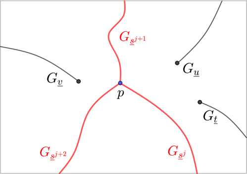
Figure 8. Sketch illustrating the statement of Lemma 5.8.

Proof.

We first prove the corresponding statement on the Riemann sphere (just replace $\mathbb{C}_{{f}^{{{\infty}}}}$ by $\hat{\mathbb{C}}$ in the statement of the lemma). Also, note that the connected components of $X\setminus\bigcup_{i}\operatorname{cl}_{X}(G_{\underline{s}^{i}})$ are the same for $X=\mathbb{C}$ and $X=\hat{\mathbb{C}}$ because $\infty\in\operatorname{cl}_{\hat{\mathbb{C}}}(G_{\underline{s}^{i}})$. By Theorem 5.7, the set $\hat{\mathbb{C}}\setminus(\operatorname{cl}_{\hat{\mathbb{C}}}(G_{\underline{s}^{1}})\cup\operatorname{cl}_{\hat{\mathbb{C}}}(G_{\underline{s}^{2}}))$ consists of precisely two connected components. Assume that $\hat{\mathbb{C}}\setminus\bigcup_{i\leq m}\operatorname{cl}_{\hat{\mathbb{C}}}(G_{\underline{s}^{i}})$ consists of precisely $m$ components $D_{1},\ldots,D_{m}$ for some $m<n$. As $G_{\underline{s}^{m+1}}$ is connected by Theorem 3.9, we have $G_{\underline{s}^{m+1}}\subset D_{j}$ for some $j$. The set $C:=\hat{\mathbb{C}}\setminus D_{j}$ is a non-separating continuum, and we have $C\cap\operatorname{cl}_{\hat{\mathbb{C}}}(G_{\underline{s}^{m+1}})=\{p,\infty\}$. By Theorem 5.7, the complement $\hat{\mathbb{C}}\setminus(C\cup\operatorname{cl}_{\hat{\mathbb{C}}}(G_{\underline{s}^{m+1}}))=\tilde{D}_{j}\cup\tilde{D}_{m+1}$ consists of precisely two connected components $\tilde{D}_{j}$ and $\tilde{D}_{m+1}$. Setting $\tilde{D}_{i}=D_{i}$ for $i\neq j$, we obtain

$$\hat{\mathbb{C}}\setminus\bigcup_{1\leq m+1}\operatorname{cl}_{\hat{\mathbb{C}}}(G_{\underline{s}^{i}})=\mathop{\vphantom{\bigcup}\mathchoice{\leavevmode\vtop{\halign{\hfil$\m@th\displaystyle#$\hfil\cr\bigcup\cr\cdot\crcr}}}{\leavevmode\vtop{\halign{\hfil$\m@th\textstyle#$\hfil\cr\bigcup\cr\cdot\crcr}}}{\leavevmode\vtop{\halign{\hfil$\m@th\scriptstyle#$\hfil\cr\bigcup\cr\cdot\crcr}}}{\leavevmode\vtop{\halign{\hfil$\m@th\scriptscriptstyle#$\hfil\cr\bigcup\cr\cdot\crcr}}}}\displaylimits_{i\leq m+1}\tilde{D}_{i},$$

where the $\tilde{D}_{i}$ are simply connected domains. It follows by induction that
$\hat{\mathbb{C}}\setminus\bigcup_{i}\operatorname{cl}_{\hat{\mathbb{C}}}(G_{\underline{s}^{i}})$ consists of precisely $n$ connected components.

To show the second statement of the lemma, choose $N$ large enough such that the fundamental tails $\tau_{N}(\underline{t})$ and $\tau_{N}(\underline{u})$ as well as the $\tau_{N}(\underline{s}^{i})$ ($i\in\{1,\ldots,n\}$) have disjoint closures. Choose $R>0$ such that

$$\bigcup_{i}\overline{G_{\underline{s}^{i}}}\subset\overline{D_{R}(p)\cup\bigcup_{i}\tau_{N}(\underline{s}^{i})}=:A.$$

The topology at $\infty$ is simple: the complement $\mathbb{C}\setminus A$ has precisely $n$ unbounded connected components and the unbounded components of $\tau_{N}(\underline{t})\setminus A$ and $\tau_{N}(\underline{u})\setminus A$ are contained in the same connected component of $\mathbb{C}\setminus A$ if and only if there exists an index $j\in\{1,\ldots,n\}$ such that $\underline{s}^{j}\prec\underline{t}\prec\underline{s}^{j+1}$ as well as $\underline{s}^{j}\prec\underline{u}\prec\underline{s}^{j+1}$. As all sufficiently large points of a dreadlock lie in the corresponding fundamental tail, the result easily translates to the case of dreadlocks.

Lastly, we want to see that the lemma also holds in $\mathbb{C}_{{f}^{{{\infty}}}}$. Given a point $q\in\mathbb{C}_{{f}^{{{\infty}}}}\setminus\mathbb{C}$, there exists a small connected neighborhood $U\subset\mathbb{C}_{{f}^{{{\infty}}}}$ of $q$ satisfying $U\cap\operatorname{cl}_{\mathbb{C}_{{f}^{{{\infty}}}}}(G_{\underline{s}^{i}})=\emptyset$ for all $i\in\{1,\ldots,n\}$. Therefore, adding the points at infinity does not lead to further connected components. ∎

The content of Lemma 5.8 is valid in a much more general context, namely for all post-singularly bounded entire functions and all bounded external addresses, and the proof works exactly the same. More precisely, using the original definition [BRG20, Corollary and Definition 6.4] of landing of dreadlocks, the following holds true:

Corollary 5.9 (Separation properties of dreadlocks).

Let $f$ be a post-singularly bounded entire function, and let $\underline{s}^{1},\ldots,\underline{s}^{n}$ be bounded external addresses indexed according to their cyclic order such that the dreadlocks $G_{\underline{s}^{1}},\ldots,G_{\underline{s}^{n}}$ land together at a point $p\in\mathcal{J}(f)$. Then $\mathbb{C}\setminus\bigcup_{i}\operatorname{cl}(G_{\underline{s}^{i}})$ consists of precisely $n$ connected components.

Two dreadlocks $G_{\underline{t}},G_{\underline{u}}\notin\{G_{\underline{s}^{1}},\ldots,G_{\underline{s}^{n}}\}$ are contained in the same connected component of $\mathbb{C}\setminus\bigcup_{i}\operatorname{cl}(G_{\underline{s}^{i}})$ if and only if there is an index $j$ such that $\underline{s}^{j}\prec\underline{t}\prec\underline{s}^{j+1}$ and $\underline{s}^{j}\prec\underline{u}\prec\underline{s}^{j+1}$ hold.

Proof.

By [BRG20, Theorem 7.1], a single bounded-address dreadlock that lands in the plane does not separate $\mathbb{C}$. Therefore, the proof of Lemma 5.8 is valid in this more general case. ∎

We also need to consider dreadlocks that land together at a transcendental singularity $p\in\mathcal{J}(\widehat{f})\setminus\mathcal{J}(f)$. Already a single dreadlock that lands at $p$ separates the complex plane (see Figure 9). Yet, if we only consider infinite sets of dreadlocks that land at $p$, a result analogous to Lemma 5.8 is valid. For the proof, we need the following result, see [Mun00, Exercise 11 in $\S$ 26].

Lemma 5.10 (Nested sequences of compacts).

Let $X$ be a Hausdorff space, and let $(C_{n})_{n=0}^{\infty}$ be a nested sequence of non-empty compact sets $C_{n}\subset X$. Then

$$C:=\bigcap_{n\geq 0}C_{n}\neq\emptyset,$$

and $C$ is compact. If each $C_{n}$ is connected, then $C$ is also connected.∎

Remark (Dreadlocks landing at transcendental singularities).

Given a transcendental singularity $p\in\mathcal{J}(\widehat{f})\setminus\mathcal{J}(f)$, it follows from the fact that $p$ is a logarithmic singularity that the ordered set of the countably many dreadlocks that land at $p$ is order-isomorphic to $\mathbb{Z}$. Hence, we may denote them as $\{G_{\underline{s}^{i}}\}_{i\in\mathbb{Z}}$ where the $\underline{s}^{i}$ are indexed according to their cyclic order. Furthermore, it follows from the mapping properties of $f$ that for every $\underline{s}\notin\{\underline{s}^{i}\}_{i\in\mathbb{Z}}$ there exists an index $j\in\mathbb{Z}$ such that $\underline{s}^{j}\prec\underline{s}\prec\underline{s}^{j+1}$. Note that these properties fail, in general, if the function has infinitely many singular values.

Lemma 5.11 (Dreadlock separation II).

Let $p\in\mathcal{J}(\widehat{f})\setminus\mathcal{J}(f)$, and let $\{G_{\underline{s}^{i}}\}_{i\in\mathbb{Z}}$ be a set of distinct dreadlocks that land at $p$ indexed according to their cyclic order. Two dreadlocks $G_{\underline{t}},G_{\underline{u}}\notin\{G_{\underline{s}^{i}}\}_{i\in\mathbb{Z}}$ are contained in the same connected component of $\mathbb{C}_{{f}^{{{\infty}}}}\setminus\bigcup_{i\in\mathbb{Z}}\operatorname{cl}_{\mathbb{C}_{{f}^{{{\infty}}}}}(G_{\underline{s}^{i}})$ if and only if there exists an index $j$ such that $\underline{s}^{j}\prec\underline{t}\prec\underline{s}^{j+1}$ and $\underline{s}^{j}\prec\underline{u}\prec\underline{s}^{j+1}$ hold.

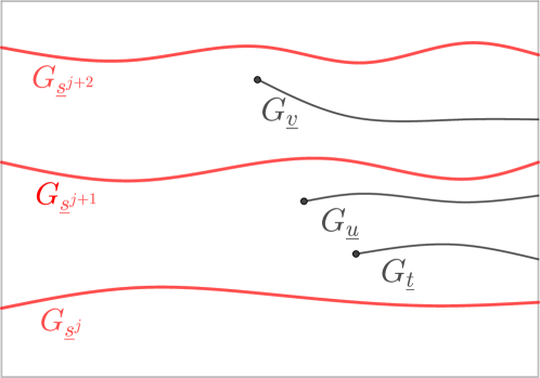
Figure 9. Sketch illustrating the statement of Lemma 5.11.

Proof.

Choose $l>0$ such that $q:=\widehat{f}^{\circ j}(p)\in\mathbb{C}$, and choose $\varepsilon>0$ such that $\overline{D_{\varepsilon}(q)}\cap P(f)=\{q\}$. Let $V\subset\mathbb{C}_{{f}^{{{\infty}}}}$ be the connected component of $\widehat{f}^{-l}(\overline{D_{\varepsilon}(q)})$ containing $p$.

First, assume that $\underline{s}^{j}\prec\underline{t}\prec\underline{s}^{j+1}$ and $\underline{s}^{j}\prec\underline{u}\prec\underline{s}^{j+1}$ for some $j\in\mathbb{Z}$. By Lemma 5.2, there exists an $N>0$ such that the fundamental tails $\tau_{N}(\underline{t})$ and $\tau_{N}(\underline{u})$ as well as the $\tau_{N}(\underline{s}^{i})$ ($i\in\mathbb{Z}$) have disjoint closures and

$$\bigcup_{i\in\mathbb{Z}}G_{\underline{s}^{i}}\subset\bigcup_{i\in\mathbb{Z}}\overline{\tau_{N}(\underline{s}^{i})}\cup V=:A.$$

As $\underline{s}^{i}\prec\underline{s}^{j}\prec\underline{s}^{j+1}$ for all $i\in\mathbb{Z}\setminus\{j,j+1\}$, there exists for all $R>0$ an arc $\gamma\colon[0,1]\to\mathbb{C}$ satisfying $\gamma(0)\in\partial\tau_{N}(\underline{s}^{j})$, $\gamma(1)\in\partial\tau_{N}(\underline{s}^{j+1})$, $\gamma((0,1))\cap A=\emptyset$, and $|\gamma(t)|\geq R$ for all $t\in[0,1]$. For $R$ large enough, the arc $\gamma$ intersects both $G_{\underline{t}}$ and $G_{\underline{u}}$. As $\gamma((0,1))\subset\mathbb{C}\setminus A\subset\mathbb{C}\setminus\bigcup_{i\in\mathbb{Z}}G_{\underline{s}^{i}}$, this shows that $G_{\underline{t}}$ and $G_{\underline{u}}$ are contained in the same connected component of $\mathbb{C}\setminus\bigcup_{i\in\mathbb{Z}}G_{\underline{s}^{i}}$ and a fortiori in the same connected component of $\mathbb{C}_{{f}^{{{\infty}}}}\setminus\bigcup_{i\in\mathbb{Z}}\operatorname{cl}_{\mathbb{C}_{{f}^{{{\infty}}}}}(G_{\underline{s}^{i}})$.

Conversely, assume that there exists a $j\in\mathbb{Z}$ such that $\underline{t}\prec\underline{s}^{j}\prec\underline{u}\prec\underline{s}^{j+1}$. By Lemma 5.2, there exists an $N\geq 1$ and a monotonically decreasing sequence $(\varepsilon_{n})_{n=N}^{\infty}$ such that $0<\varepsilon_{n}<\varepsilon$, $\lim_{n\to\infty}\varepsilon_{n}=0$, and

$$\bigcup_{i\in\mathbb{Z}}G_{\underline{s}^{i}}\subset\bigcup_{i\in\mathbb{Z}}\overline{\accentset{\infty}{\tau}_{n}(\underline{s}^{i})}\cup V_{n}=:A_{n},$$

where the $A_{n}$ form a nested sequence of closed sets. Here $V_{n}$ denotes the connected component of $f^{-l}(\overline{D_{\varepsilon_{n}}(q)})$ contained in $V$. For all sufficiently large $n$, the dreadlocks $G_{\underline{t}}$ and $G_{\underline{u}}$ are contained in distinct connected components of $\mathbb{C}\setminus A_{n}$.

Assume that $G_{\underline{t}}$ and $G_{\underline{u}}$ are contained in the same connected component $U$ of $\mathbb{C}\setminus\bigcup_{i\in\mathbb{Z}}G_{\underline{s}^{i}}$. Then there exists an arc $\gamma\colon[0,1]\to U$ satisfying $\gamma(0)\in G_{\underline{t}}$ and $\gamma(1)\in G_{\underline{u}}$. By construction, we have $\bigcap_{n\geq 1}A_{n}=\bigcup_{i\in\mathbb{Z}}G_{\underline{s}^{i}}$. As $G_{\underline{u}}$ and $G_{\underline{t}}$ are contained in distinct connected components of $A_{n}$ for all $n\geq 1$, we have $C_{n}:=\gamma\cap A_{n}\neq\emptyset$ for all $n\geq 1$. It follows from Lemma 5.10 that $\gamma\cap\bigcup_{i\in\mathbb{Z}}G_{\underline{s}^{i}}\neq\emptyset$ contradicting our assumptions. Hence, the dreadlocks $G_{\underline{t}}$ and $G_{\underline{u}}$ are contained in distinct connected components of $\mathbb{C}\setminus\bigcup_{i\in\mathbb{Z}}G_{\underline{s}^{i}}$. As every $q\in\mathbb{C}_{{f}^{{{\infty}}}}\setminus(\mathbb{C}\cup\{p\})$ has a neighborhood $U$ that satisfies $U\cap G_{\underline{s}^{i}}=\emptyset$ for all $i\in\mathbb{Z}$, the dreadlocks $G_{\underline{t}}$ and $G_{\underline{u}}$ are also contained in distinct connected components of $\mathbb{C}_{{f}^{{{\infty}}}}\setminus\bigcup_{i\in\mathbb{Z}}\operatorname{cl}_{\mathbb{C}_{{f}^{{{\infty}}}}}(G_{\underline{s}^{i}})$

∎

Let us summarize the content of Lemmas 5.8 and 5.11.

Corollary 5.12.

Let $p\in\mathcal{J}(\widehat{f})$ be (pre-)periodic, and let $\{G_{\underline{s}^{i}}\}_{i\in I}$ be the set of dreadlocks that land at $p$ indexed according to their cyclic order, where we either have $I=\mathbb{Z}$ or $I=\mathbb{Z}/m\mathbb{Z}$ for some $m\geq 1$.

Then every connected component of $W:=\mathbb{C}_{{f}^{{{\infty}}}}\setminus\bigcup_{L(\underline{s})=p}\operatorname{cl}_{\mathbb{C}_{{f}^{{{\infty}}}}}(G_{\underline{s}})$ is open and simply connected.

Furthermore, two dreadlocks $G_{\underline{t}},G_{\underline{u}}\notin\{G_{\underline{s}^{i}}\}_{i\in I}$ are contained in the same connected component of $W$ if and only if $\underline{s}^{j}\prec\underline{t}\prec\underline{s}^{j+1}$ and $\underline{s}^{j}\prec\underline{u}\prec\underline{s}^{j+1}$ for some $j\in I$.

5.3. Extended Dreadlocks

Post-singular points in the Fatou set cannot be landing points of dreadlocks. We still obtain a dynamically meaningful set that connects a post-singular point in the Fatou set to infinity by extending a dreadlock that lands at a boundary point of the corresponding Fatou component with an internal ray of the component.

Notation.

Let $U$ be a component of $\mathcal{F}(\widehat{f})$, and let $q\in\partial_{\mathbb{C}_{{f}^{{{\infty}}}}}U$. By Subsection 3.1, in particular Lemma 3.1, there exists at most one internal ray of $U$ that lands at $q$. We denote this ray (if it exists) by $\beta_{U}[q]$.

Definition 5.13 (Extended dreadlock).

Let $p\in\mathbb{C}_{{f}^{{{\infty}}}}$ be the center of a Fatou component $U(p)$. An extended dreadlock that lands at $p$ consists of a dreadlock $G_{\underline{s}}$ that lands at a (pre-)periodic boundary point $q=L(\underline{s})\in\partial_{\mathbb{C}_{{f}^{{{\infty}}}}}U(p)$, extended by the internal ray $\beta_{U(p)}[q]$ of $U(p)$ that lands at $q$. The external address of the extended dreadlock $G_{\underline{s}}[p]$ is by definition $\underline{s}$. We denote this extended dreadlock by $G_{\underline{s}}[p]:=\beta_{U(p)}[q]\cup\operatorname{cl}_{\mathbb{C}_{{f}^{{{\infty}}}}}(G_{\underline{s}})$.

In general, there are infinitely many extended dreadlocks that land at any given Fatou center $p\in\mathcal{F}(\widehat{f})$: the Fatou component $U(p)$ has infinitely many (pre-)periodic boundary points, and all of them are landing points of (pre-)periodic dreadlocks.

Convention.

Let $G_{\underline{s}}$ be a dreadlock that lands at a (pre-)periodic point $p=L(\underline{s})\in\mathbb{C}_{{f}^{{{\infty}}}}$. In order to have a unified notation for dreadlocks and extended dreadlocks, we use $G_{\underline{s}}[p]:=G_{\underline{s}}$ as an equivalent notion for the dreadlock $G_{\underline{s}}$.

Let $p\in\mathbb{C}_{{f}^{{{\infty}}}}$ be the center of a Fatou component $U(p)$, and let $q\in\partial_{\mathbb{C}_{{f}^{{{\infty}}}}}U(p)$ be (pre-)periodic. As in the statement of Corollary 5.12, let $\{G_{\underline{s}^{i}}\}_{i\in I}$ be the set of dreadlocks that land at $q$ indexed according to their cyclic order, and let $W:=\mathbb{C}_{{f}^{{{\infty}}}}\setminus\bigcup_{L(\underline{s})=p}\operatorname{cl}_{\mathbb{C}_{{f}^{{{\infty}}}}}(G_{\underline{s}})$. Let $V$ be the connected component of $W$ containing $U(p)$. By Corollary 5.12, there exists an index $j\in I$ such that $G_{\underline{s}^{j}}\prec G_{\underline{t}}\prec G_{\underline{s}^{j+1}}$ for all dreadlocks $G_{\underline{t}}\subset V$.

Definition 5.14 (Left and right supporting dreadlocks).

We call $G_{\underline{s}^{j}}$ the left supporting dreadlock of $U(q)$ at $p$, and $G_{\underline{s}^{j+1}}$ the right supporting dreadlock of $U(q)$ at $p$; see also Figure 10.

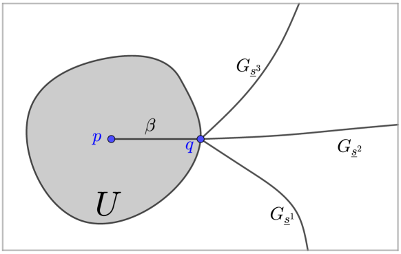
Figure 10. Sketch of the left and right supporting dreadlocks $G_{\underline{s}^{3}}$ and $G_{\underline{s}^{1}}$ at a boundary point $q\in\partial U$ of the Fatou component $U=U(p)$. We obtain an extended dreadlock by concatenating $G_{\underline{s}^{i}}$ with $\beta$.

Proposition 5.15 (Topology of extended dreadlocks).

Let $G_{\underline{s}}[p]$ be an (extended) dreadlock, and let $q:=L(\underline{s})$. If $p,q\in\mathbb{C}$, then $\operatorname{cl}_{\hat{\mathbb{C}}}(G_{\underline{s}}[p])$ does not separate the Riemann sphere.

Proof.

For $p\in\mathcal{J}(f)$, this is the content of Proposition 5.4. For $p\in\mathcal{F}(f)$, both $\operatorname{cl}_{\hat{\mathbb{C}}}(\beta_{U(p)}[q])$ and $\operatorname{cl}_{\hat{\mathbb{C}}}(G_{\underline{s}})$ do not separate the Riemann sphere, and the intersection $\operatorname{cl}_{\hat{\mathbb{C}}}(\beta_{U(p)}[q])\cap\operatorname{cl}_{\hat{\mathbb{C}}}(G_{\underline{s}})=\{q\}$ is a singleton. It follows from Theorem 5.7 that $G_{\underline{s}}[p]$ does not separate the Riemann sphere. ∎

A result analogous to Corollary 5.12 is valid for extended dreadlocks supporting the same Fatou component.

Lemma 5.16 (Dreadlock separation III).

Let $p\in\mathcal{F}(\widehat{f})$ be the center of the Fatou component $U\subset\mathcal{F}(\widehat{f})$. Let $\{G_{\underline{s}^{i}}\}_{i\in I}$ be dreadlocks such that the landing points $L(\underline{s}^{i})\in\partial U$ are distinct and satisfy $L(\underline{s}^{i})\in\mathbb{C}$. If $p\in\mathbb{C}$, we require that $I=\mathbb{Z}/m\mathbb{Z}$ for some $m\geq 1$. If $p\in\mathbb{C}_{{f}^{{{\infty}}}}\setminus\mathbb{C}$, we require that $I=\mathbb{Z}$ and that the set $\{L(\underline{s}^{i})\}$ of landing points is discrete. In both cases, we assume that the dreadlocks are indexed according to their cyclic order.

Let $G_{\underline{t}}[q]$ and $G_{\underline{u}}[r]$ be (extended) dreadlocks such that

$$G_{\underline{t}}[q]\cap G_{\underline{s}^{i}}[p]=G_{\underline{u}}[r]\cap G_{\underline{s}^{i}}[p]=\emptyset\leavevmode\nobreak\ \leavevmode\nobreak\ \leavevmode\nobreak\ \text{for all}\leavevmode\nobreak\ i\in I.$$

Then the extended dreadlocks $G_{\underline{t}}[q]$ and $G_{\underline{t}}[r]$ are contained in the same connected component of $\mathbb{C}_{{f}^{{{\infty}}}}\setminus\bigcup_{i\in I}\operatorname{cl}_{\mathbb{C}_{{f}^{{{\infty}}}}}(G_{\underline{s}^{i}}[p])$ if and only if there exists an index $j\in I$ such that $\underline{s}^{j}\prec\underline{t}\prec\underline{s}^{j+1}$ as well as $\underline{s}^{j}\prec\underline{u}\prec\underline{s}^{j+1}$.

Proof.

The proof works similarly to the proofs of Lemma 5.8 and Lemma 5.11. ∎

6. Dynamic Partitions

We construct, for a given psf entire map $f$, a dynamic partition by choosing for each singular value an (extended) dreadlock that lands at this value, and taking the preimage of the complement: this way, the (extended) complex plane is partitioned into components called partition sectors that map univalently onto the entire extended plane, minus the chosen (extended) dreadlocks.

Definition 6.1 (Dynamic partition).

For a given psf entire map $f$, let $S(f)=\{a_{1},\ldots,a_{n}\}$ be the set of its singular values. Choose for every $a_{i}\in S(f)$ an (extended) dreadlock $G_{\underline{s}^{i}}[a_{i}]$ such that $\overline{G_{\underline{s}^{i}}[a_{i}]}\cap\overline{G_{\underline{s}^{j}}[a_{j}]}=\emptyset$ for $i\neq j$. For all $a_{i}\in S(f)\cap\mathcal{F}(f)$, we require that $L(\underline{s}^{i})\in\mathbb{C}$ and that $\underline{s}^{i}$ is the address of the left supporting dreadlock for $U(a_{i})$ at $L(\underline{s}^{i})$ (see Definition 5.14). Define the base domain

$$B:=\mathbb{C}\setminus\bigcup_{a_{i}\in S(f)}\overline{G_{\underline{s}^{i}}[a_{i}]}$$

and define the dynamic partition for $f$ (with respect to the chosen dreadlocks) as the collection of connected components of $f^{-1}(B)$ and denote it by $\mathcal{D}$; see Figure 11.

An element $D\in\mathcal{D}$ (i.e., a component of $f^{-1}(B)$) is called a partition sector. The set

$$\partial\mathcal{D}:=f^{-1}(\bigcup_{a_{i}\in S(f)}\overline{G_{\underline{s}^{i}}[a_{i}]})\subset\mathbb{C}$$

is called the boundary of $\mathcal{D}$.

We sometimes write $\mathcal{D}=\mathcal{D}(\{G_{\underline{s}^{i}}[a_{i}]\})$ if we want to emphasize the (extended) dreadlocks used to define the partition $\mathcal{D}$.

Remark.

Since we choose a single dreadlock for each singular value, and in such a way that they are disjoint, the base domain $B$ is always simply connected and free of singular values. Therefore, the restriction $f\colon D\to B$ for any partition sector is biholomorphic. We are going to prove this in more detail in Lemma 6.3.

Taking left supporting dreadlocks for singular values in the Fatou set is just a convention that allows for a more convenient description of which (pre-)periodic dreadlocks land together in terms of itineraries.

Since we also want to assign itineraries to points at infinity, it is useful to extend the base domain to include $\mathbb{C}_{{f}^{{{\infty}}}}\setminus\mathbb{C}$.

Definition 6.2 (Extended dynamic partition).

Let $\mathcal{D}=\mathcal{D}(\{G_{\underline{s}^{i}}[a_{i}]\})$ be a dynamic partition for $f$. We call

$$\widehat{B}:=\mathbb{C}_{{f}^{{{\infty}}}}\setminus\bigcup_{a_{i}\in S(f)}\operatorname{cl}_{\mathbb{C}_{{f}^{{{\infty}}}}}(G_{\underline{s}^{i}}[a_{i}])$$

the extended base domain of $\mathcal{D}$, and define the extended dynamic partition $\widehat{\mathcal{D}}$ as the collection of connected components of $\widehat{f}^{-1}(\widehat{B})$. An element $\widehat{D}\in\widehat{\mathcal{D}}$ is called an extended partition sector. We also write

$$\partial\widehat{\mathcal{D}}:=\widehat{f}^{-1}(\bigcup_{a_{i}\in S(f)}\operatorname{cl}_{\mathbb{C}_{{f}^{{{\infty}}}}}(G_{\underline{s}^{i}}[a_{i}]))$$ (2)

for the boundary of the extended partition $\widehat{\mathcal{D}}$.

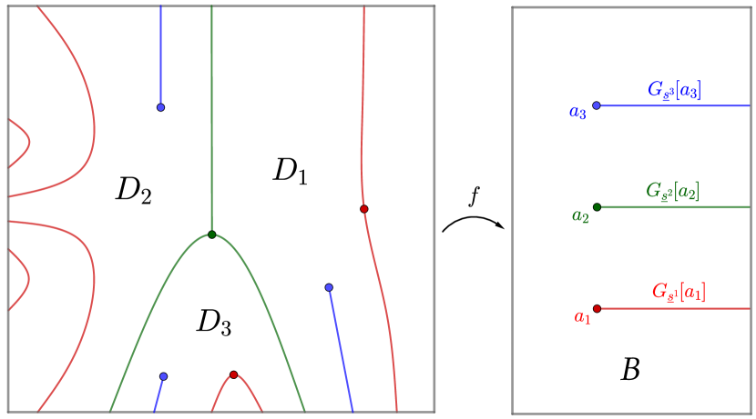
Figure 11. Sketch of some base domain (right), together with the corresponding dynamic partition (left). In the very left, we see (in red) parts of dreadlocks that land together at some point at infinity. We have drawn the dreadlocks as straight lines in this image, although they are, in general, topologically far more complicated. However, regarding the features that are essential for dynamic partitions, a straight line is equivalent to a more complicated dreadlock.

An essential property of dynamic partitions is that the base domain is evenly covered.

Lemma 6.3 (Covering properties of dynamic partitions).

Let $f$ be a psf entire function, and let $\mathcal{D}$ be a dynamic partition for $f$. Every partition sector $D\in\mathcal{D}$ is mapped biholomorphically onto $B[\mathcal{D}]$. Every extended partition sector $\widehat{D}\in\widehat{\mathcal{D}}$ is mapped homeomorphically onto $B[\widehat{\mathcal{D}}]$.

Proof.

As we required $L(\underline{s}^{i})\in\mathbb{C}$ for all $i$, it follows from Proposition 5.15 that every individual $\operatorname{cl}_{\hat{\mathbb{C}}}(G_{\underline{s}^{i}}[a_{i}])$ does not separate the sphere. As the continua $\operatorname{cl}_{\hat{\mathbb{C}}}(G_{\underline{s}^{i}}[a_{i}])$ only intersect each other at $\infty$, Theorem 5.7 implies that their union also does not separate the sphere, so their complement $B[\mathcal{D}]$ is simply connected. We have $B[\mathcal{D}]\cap S(f)=\emptyset$, so $f$ is a covering over $B[\mathcal{D}]$. This shows that every partition sector $D\in\mathcal{D}$ is mapped biholomorphically onto $B[\mathcal{D}]$.

None of the (extended) dreadlocks $G_{\underline{s}^{i}}[a_{i}]$ accumulates at any of the points in $\mathbb{C}_{{f}^{{{\infty}}}}\setminus\mathbb{C}$, as all sufficiently large points of $G_{\underline{s}^{i}}[a_{i}]$ are contained in a fundamental tail $\tau_{N}$ of level $N$ for all $N\geq 1$, see Lemma 5.2. Therefore, every $p\in\mathbb{C}_{{f}^{{{\infty}}}}\setminus\mathbb{C}$ has a simply connected punctured neighborhood $V\subset B[\mathcal{D}]$. By the first paragraph, for a given partition sector $D$, there is a unique preimage component $U\subset D$ of $V$ under $f$. Therefore, the point $p$ has a unique preimage $q$ in the extended partition sector $\widehat{D}$. ∎

The boundary of a dynamic partition consists of the preimages of the (extended) dreadlocks $G_{\underline{s}^{i}}[a_{i}]$, so every dreadlock that is not one of these preimages is entirely contained in some partition sector. As dreadlocks are distinguished by external addresses, a dynamic partition of the plane also partitions the space of external addresses: We call two external addresses equivalent if the associated dreadlocks are contained in the same partition sector. We want to describe this equivalence relation on $\mathbf{S}\setminus\sigma^{-1}(\{\underline{s}^{1},\ldots,\underline{s}^{n}\})$. To this end, we need the concept of (un)linked sets of external addresses.

Definition 6.4 (Unlinked addresses).

We call two sets $T,U\subset\mathbf{S}$ of external addresses unlinked if $T\cap U=\emptyset$ and there do not exist addresses $\underline{t}^{1},\underline{t}^{2}\in T$ and $\underline{u}^{1},\underline{u}^{2}\in U$, such that

$$\underline{t}^{1}\prec\underline{u}^{1}\prec\underline{t}^{2}\prec\underline{u}^{2}.$$

Otherwise, $T$ and $U$ are called linked.

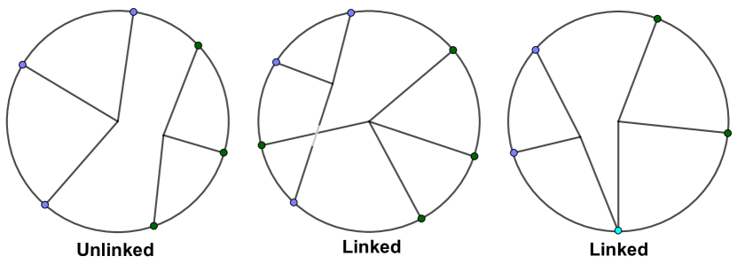
Figure 12. Illustration of linked and unlinked sets of addresses.

The motivation for this concept comes from dreadlocks that land together. Using the definition of unlinked addresses, Corollary 5.12 can be restated as follows: given a (pre-)periodic $p\in\mathcal{J}(\widehat{f})$, two dreadlocks $G_{\underline{t}}$ and $G_{\underline{u}}$ that do not land at $p$ are contained in the same component of $\mathbb{C}_{{f}^{{{\infty}}}}\setminus\bigcup_{L(\underline{s})=p}\operatorname{cl}_{\mathbb{C}_{{f}^{{{\infty}}}}}(G_{\underline{s}})$ (i.e. they are not separated by two dreadlocks landing at $p$) if and only if the sets $\{\underline{s}\colon L(\underline{s})=p\}$ and $\{\underline{t},\underline{u}\}$ are unlinked. A nice visualization of unlinked addresses is obtained by passing to the circle of addresses $\overline{\mathbf{S}}$ that is the order completion of $\mathbf{S}$ (see the paragraph after Definition 3.13). The extended plane $\mathbb{C}\cup\overline{\mathbf{S}}$ is homeomorphic to the closed unit disk $\overline{\mathbb{D}}$, and two subsets $T$ and $U$ of $\overline{\mathbf{S}}$ are unlinked if and only if there are connected subsets $X,Y\subset\mathbb{C}\cup\overline{\mathbf{S}}$ such that $T\subset X$ and $U\subset Y$, see [BFH92, Lemma 2.5] and Figure 12.

Let $\underline{s}^{1},\ldots,\underline{s}^{n}$ be the external addresses of the (extended) dreadlocks that land at the singular values of $f$ as in Definition 6.1, ordered so that $\underline{s}^{1}<\underline{s}^{2}<\ldots<\underline{s}^{n}$ in the linear order defined in Subsubsection 3.2.2. For a point $c\in\widehat{f}^{-1}(S(f))$ with $\widehat{f}(c)=a_{j}$, we define

$$\mathcal{C}(c):=\{\underline{c}\in\mathbf{S}\colon L(\underline{c})=c\leavevmode\nobreak\ \text{and}\leavevmode\nobreak\ \sigma(\underline{c})=\underline{s}^{j}\}\subset\mathbf{S}\;;$$

these are all preimage external addresses to the chosen external addresses at the singular values, including those that belong to regular preimages of the singular values.

Using this definition, we can now give a purely combinatorial definition of external addresses that belong to dreadlocks in the same partition sector: we give the definition now and justify it in Proposition 6.7.

Definition 6.5 (Dynamic Partitions of $\mathbf{S}$).

Two external addresses $\underline{t},\underline{u}\in\mathbf{S}\setminus\sigma^{-1}(\{\underline{s}^{1},\ldots,\underline{s}^{n}\})$ are called unlink equivalent if $\mathcal{C}(c)$ and $\{\underline{t},\underline{u}\}$ are unlinked for all $c\in\widehat{f}^{-1}(S(f))$. We call the resulting set $\mathcal{I}$ of equivalence classes the dynamic partition of $\mathbf{S}$ (with respect to $\{\underline{s}^{1},\ldots,\underline{s}^{n}\}$). The elements $I\in\mathcal{I}$ are called partition sectors of $\mathbf{S}$.

This definition is such that there is a natural correspondence between the partition sectors of the dynamic partition $\mathcal{D}$ of the complex plane and the dynamic partition $\mathcal{I}$ of the space of external addresses.

Lemma 6.6 (Sector boundary).

Let $\mathcal{D}$ be a dynamic partition and $D\in\mathcal{D}$ a partition sector. For every singular value $a_{i}$, the intersection

$$\partial_{\mathbb{C}_{{f}^{{{\infty}}}}}D\cap\widehat{f}^{-1}(\{a_{i}\})$$

is a single point that we call $c_{i}$. We have

$$\partial_{\mathbb{C}_{{f}^{{{\infty}}}}}D\subset\bigcup_{i\in\{1,\ldots,n\}}\bigcup_{\underline{s}\in\mathcal{C}(c_{i})}\operatorname{cl}_{\mathbb{C}_{{f}^{{{\infty}}}}}(G_{\underline{s}}[c_{i}]).$$ (3)

and thus

$$D=\bigcap_{i\in\{1,\ldots,n\}}W_{i},$$ (4)

where $W_{i}$ is the complementary component of $\bigcup_{\underline{s}\in\mathcal{C}(c_{i})}\overline{G_{\underline{s}}[c_{i}]}$ that contains $D$.

If $p$ and $q$ are two points in different partition sectors, then there exists a $c_{i}$ such that $p$ and $q$ are contained in different components of $\mathbb{C}_{{f}^{{{\infty}}}}\setminus\bigcup_{\underline{s}\in\mathcal{C}(c)}\operatorname{cl}_{\mathbb{C}_{{f}^{{{\infty}}}}}(G_{\underline{s}}[c])$.

Proof.

Choose pairwise disjoint domains $U_{i}\supset G_{\underline{s}^{i}}[a_{i}]$ such that each $U_{i}$ is simply connected. Since $\widehat{f}\colon\widehat{D}\to\widehat{f}(\widehat{D})=\widehat{B}$ is a homeomorphism, $D$ intersects a single preimage component of each $U_{i}$.

Since $\partial\widehat{\mathcal{D}}=\mathbb{C}_{{f}^{{{\infty}}}}\setminus\bigcup_{a_{i}\in S(f)}\operatorname{cl}_{\mathbb{C}_{{f}^{{{\infty}}}}}(G_{\underline{s}^{i}}[a_{i}])$ (see (2)), $\partial_{\mathbb{C}_{{f}^{{{\infty}}}}}D$ consists of preimages of those $\operatorname{cl}_{\mathbb{C}_{{f}^{{{\infty}}}}}(G_{\underline{s}^{i}}[a_{i}])$ that land at the $c_{i}$, and this is (3).

It follows that $D$ is separated from its complement by pairs of dreadlocks that land at the various $c_{i}$, and this shows (4) and the final claim. ∎

Using this lemma, we can establish the natural correspondence between partition sectors of the plane and of the space of external addresses.

Proposition 6.7 (Sector correspondence).

Consider two dreadlocks $G_{\underline{t}}$ and $G_{\underline{u}}$ that are both not on the boundary of a partition sector. They are contained in the same sector of $\mathcal{D}$ if and only if $\underline{t}$ and $\underline{u}$ are contained in the same sector of $\mathcal{I}$.

Proof.

First, assume that $G_{\underline{t}}$ and $G_{\underline{u}}$ are contained in the same sector of $\mathcal{D}$, and assume to the contrary that $\mathcal{C}(c)$ and $\{\underline{t},\underline{u}\}$ are linked for some $c\in\widehat{f}^{-1}(S(f))$. By definition, there are external addresses $\underline{c}^{1},\underline{c}^{2}\in\mathcal{C}(c)$ such that $\underline{c}^{1}\prec\underline{t}\prec\underline{c}^{2}\prec\underline{u}$. The (extended) dreadlocks $G_{\underline{c}^{1}}[c]$ and $G_{\underline{c}^{2}}[c]$ land together at the point $c\in\mathbb{C}_{{f}^{{{\infty}}}}$ and are contained in $\partial\mathcal{D}$. By Lemma 5.8, Lemma 5.11, and Lemma 5.16, the dreadlocks $G_{\underline{t}}$ and $G_{\underline{u}}$ are contained in distinct connected components of $\mathbb{C}\setminus\bigcup_{\underline{s}\in\mathcal{C}(c)}\overline{G_{\underline{s}}[c]}$ and thus in distinct partition sectors, a contradiction.

Conversely, assume that $\underline{t}$ and $\underline{u}$ are unlink equivalent. If $G_{\underline{t}}$ and $G_{\underline{u}}$ were contained in distinct sectors of $\mathcal{D}$, then we could find a point $c\in\widehat{f}^{-1}(S(f))$ such that $G_{\underline{t}}$ and $G_{\underline{u}}$ are contained in distinct connected components of $\mathbb{C}\setminus\bigcup_{\underline{s}\in\mathcal{C}(c)}\overline{G_{\underline{s}}[c]}$ by Lemma 6.6. By Lemma 5.8, Lemma 5.11, and Lemma 5.16, this implies the existence of $\underline{c}^{1},\underline{c}^{2}\in\mathcal{C}(c)$ such that $\underline{c}^{1}\prec\underline{t}\prec\underline{c}^{2}\prec\underline{u}$. Hence, $\{\underline{t},\underline{u}\}$ and $\mathcal{C}(c)$ would be linked, again a contradiction. ∎

Having thus established a natural bijection between the partition sectors of $\mathcal{D}$ and $\mathcal{I}$, we write $D(I)$ and $I(D)$ for the sector $D\in\mathcal{D}$ corresponding to $I\in\mathcal{I}$ and the sector $I$ corresponding to $D$ respectively.

Proposition 6.8 (Topology of $I$).

Let $I$ be a sector of the dynamic partition $\mathcal{I}$. The restriction

$$\left.\sigma\right|_{I}\colon I\to\mathbf{S}\setminus\{\underline{s}^{1},\ldots,\underline{s}^{n}\}$$

is a bijection that preserves the cyclic order. We have

$$I=(\underline{t}^{1},\underline{t}^{2})\mathbin{\mathchoice{\leavevmode\vtop{\halign{\hfil$\m@th\displaystyle#$\hfil\cr\cup\cr\cdot\crcr}}}{\leavevmode\vtop{\halign{\hfil$\m@th\textstyle#$\hfil\cr\cup\cr\cdot\crcr}}}{\leavevmode\vtop{\halign{\hfil$\m@th\scriptstyle#$\hfil\cr\cup\cr\cdot\crcr}}}{\leavevmode\vtop{\halign{\hfil$\m@th\scriptscriptstyle#$\hfil\cr\cup\cr\cdot\crcr}}}}(\underline{t}^{3},\underline{t}^{4})\mathbin{\mathchoice{\leavevmode\vtop{\halign{\hfil$\m@th\displaystyle#$\hfil\cr\cup\cr\cdot\crcr}}}{\leavevmode\vtop{\halign{\hfil$\m@th\textstyle#$\hfil\cr\cup\cr\cdot\crcr}}}{\leavevmode\vtop{\halign{\hfil$\m@th\scriptstyle#$\hfil\cr\cup\cr\cdot\crcr}}}{\leavevmode\vtop{\halign{\hfil$\m@th\scriptscriptstyle#$\hfil\cr\cup\cr\cdot\crcr}}}}\ldots\mathbin{\mathchoice{\leavevmode\vtop{\halign{\hfil$\m@th\displaystyle#$\hfil\cr\cup\cr\cdot\crcr}}}{\leavevmode\vtop{\halign{\hfil$\m@th\textstyle#$\hfil\cr\cup\cr\cdot\crcr}}}{\leavevmode\vtop{\halign{\hfil$\m@th\scriptstyle#$\hfil\cr\cup\cr\cdot\crcr}}}{\leavevmode\vtop{\halign{\hfil$\m@th\scriptscriptstyle#$\hfil\cr\cup\cr\cdot\crcr}}}}(\underline{t}^{2n-1},\underline{t}^{2n})$$

with superscripts labeled modulo $2n$ and $\sigma(\underline{t}^{2i})=\sigma(\underline{t}^{2i+1})=\underline{s}^{i}$. There are distinct $c_{i}\in\widehat{f}^{-1}(S(f))$, $i\in\{1,\ldots,n\}$, such that $\underline{t}^{2i},\underline{t}^{2i+1}\in\mathcal{C}(c_{i})$.

Proof.

As shown in Lemma 6.3, the restriction of $f$ to $D(I)$ is a conformal isomorphism onto $\mathbb{C}\setminus\bigcup_{i=1}^{n}\overline{G_{\underline{s}^{i}}[a_{i}]}$. Therefore, every dreadlock $G_{\underline{t}}$ with $\underline{t}\notin\{\underline{s}^{1},\ldots,\underline{s}^{n}\}$ has a unique preimage in $D(I)$. By Proposition 6.7, every external address $\underline{u}\in\mathbf{S}\setminus\{\underline{s}^{1},\ldots,\underline{s}^{n}\}$ that is realized by some dreadlock has a unique preimage in $I$. Since realized addresses are dense in $\mathbf{S}$, every external address $\underline{u}\in\mathbf{S}\setminus\{\underline{s}^{1},\ldots,\underline{s}^{n}\}$ has a unique preimage in $I$. This shows that $\left.\sigma\right|_{I}$ is a bijection onto $\mathbf{S}\setminus\{\underline{s}^{1},\ldots,\underline{s}^{n}\}$. Let $G_{\underline{t}},G_{\underline{u}},G_{\underline{v}}\subset D(I)$ be distinct dreadlocks satisfying $G_{\underline{t}}\prec G_{\underline{u}}\prec G_{\underline{v}}$. As $\left.f\right|_{D_{i}}$ is a conformal map onto $B[\mathcal{D}]$ by Lemma 6.3, thus an orientation-preserving homeomorphism, we have $G_{\sigma(\underline{t})}\prec G_{\sigma(\underline{u})}\prec G_{\sigma(\underline{v})}$. On the level of external addresses, this means that $\left.\sigma\right|_{I}$ preserves the cyclic order for every triple of realized external addresses. As realized addresses are dense in $\mathbf{S}$, we conclude that $\left.\sigma\right|_{I}$ is order-preserving.

Let $\underline{s}\in\mathbf{S}\setminus\partial\mathcal{I}$ be an external address, and let $F$ be its initial entry. We have $\sigma(\underline{s})\in(\underline{s}^{j},\underline{s}^{j+1})$ for some $j$. Recall that we required $\underline{s}^{1}<\ldots<\underline{s}^{n}$ in the linear order induced by $\alpha$ (see Definition 3.14). If $j\neq n$, then we have $\underline{s}\in(F\underline{s}^{j},F\underline{s}^{j+1})$. If $j=n$, we further distinguish whether $\sigma(\underline{s})<\underline{s}^{1}$ or $\sigma(\underline{s})>\underline{s}^{1}$. In the former case, we have $\underline{s}\in(F_{p}\underline{s}^{n},F\underline{s}^{1})$, while in the latter case we have $\underline{s}\in(F\underline{s}^{n},F_{s}\underline{s}^{1})$. Hence, $\mathbf{S}\setminus\partial\mathcal{I}$ can be written as the disjoint union of intervals of the above form. Each of these intervals is fully contained in some sector of $\mathcal{I}$, and the restriction of $\sigma$ to any of these intervals preserves the cyclic order. By the above, $I$ is mapped bijectively onto $\mathbf{S}\setminus\{\underline{s}^{1},\ldots,\underline{s}^{n}\}$, so there are fundamental domains $F_{j}$ ($j\in\{1,\ldots,n\}$) such that

$$I=((F_{1})_{p}\underline{s}^{n},F_{1}\underline{s}^{1})\mathbin{\mathchoice{\leavevmode\vtop{\halign{\hfil$\m@th\displaystyle#$\hfil\cr\cup\cr\cdot\crcr}}}{\leavevmode\vtop{\halign{\hfil$\m@th\textstyle#$\hfil\cr\cup\cr\cdot\crcr}}}{\leavevmode\vtop{\halign{\hfil$\m@th\scriptstyle#$\hfil\cr\cup\cr\cdot\crcr}}}{\leavevmode\vtop{\halign{\hfil$\m@th\scriptscriptstyle#$\hfil\cr\cup\cr\cdot\crcr}}}}(F_{2}\underline{s}^{1},F_{2}\underline{s}^{2})\mathbin{\mathchoice{\leavevmode\vtop{\halign{\hfil$\m@th\displaystyle#$\hfil\cr\cup\cr\cdot\crcr}}}{\leavevmode\vtop{\halign{\hfil$\m@th\textstyle#$\hfil\cr\cup\cr\cdot\crcr}}}{\leavevmode\vtop{\halign{\hfil$\m@th\scriptstyle#$\hfil\cr\cup\cr\cdot\crcr}}}{\leavevmode\vtop{\halign{\hfil$\m@th\scriptscriptstyle#$\hfil\cr\cup\cr\cdot\crcr}}}}\ldots\mathbin{\mathchoice{\leavevmode\vtop{\halign{\hfil$\m@th\displaystyle#$\hfil\cr\cup\cr\cdot\crcr}}}{\leavevmode\vtop{\halign{\hfil$\m@th\textstyle#$\hfil\cr\cup\cr\cdot\crcr}}}{\leavevmode\vtop{\halign{\hfil$\m@th\scriptstyle#$\hfil\cr\cup\cr\cdot\crcr}}}{\leavevmode\vtop{\halign{\hfil$\m@th\scriptscriptstyle#$\hfil\cr\cup\cr\cdot\crcr}}}}(F_{n}\underline{s}^{n},(F_{n})_{s}\underline{s}^{1}).$$

Hence, we see that $I$ is of the claimed form. The last statement follows from Lemma 6.6 where the $c_{i}$ from Lemma 6.6 coincide with the $c_{i}$ in the statement of this proposition. ∎

Corollary 6.9 (Boundary correspondence).

Let $I\in\mathcal{I}$ be a partition sector. In the notation of Proposition 6.8, we have $G_{\underline{t}}\cap\overline{D(I)}\neq\emptyset$ if and only if $\underline{t}\in[\underline{t}^{2j-1},\underline{t}^{2j}]$ for some $j\in\{1,\ldots,n\}$. If $G_{\underline{t}}$ is (pre-)periodic and $G_{\underline{t}}\cap\overline{D(I)}\neq\emptyset$, we have $L(\underline{t})\in\operatorname{cl}_{\mathbb{C}_{{f}^{{{\infty}}}}}(D(I))$.

Proof.

If $\underline{t}\notin\partial\mathcal{I}$, this follows directly from Proposition 6.7. In the boundary case, this follows easily from Proposition 6.8 and Lemma 6.6. ∎

By adding either all left boundary points or all right boundary points to the sectors of $\mathcal{I}$, we obtain two full partitions of the space of external addresses.

Corollary and Definition 6.10 (Full partitions).

For a partition sector $I\in\mathcal{I}$, we set

$$I^{-}:=(\underline{t}^{1},\underline{t}^{2}]\cup(\underline{t}^{3},\underline{t}^{4}]\cup\ldots\cup(\underline{t}^{2n-1},\underline{t}^{2n}]$$

and

$$I^{+}:=[\underline{t}^{1},\underline{t}^{2})\cup[\underline{t}^{3},\underline{t}^{4})\cup\ldots\cup[\underline{t}^{2n-1},\underline{t}^{2n}),$$

where the $\underline{t}^{i}$ are the external addresses introduced in Proposition 6.8. In this way, we get two full partitions

$$\mathbf{S}=\mathop{\vphantom{\bigcup}\mathchoice{\leavevmode\vtop{\halign{\hfil$\m@th\displaystyle#$\hfil\cr\bigcup\cr\cdot\crcr}}}{\leavevmode\vtop{\halign{\hfil$\m@th\textstyle#$\hfil\cr\bigcup\cr\cdot\crcr}}}{\leavevmode\vtop{\halign{\hfil$\m@th\scriptstyle#$\hfil\cr\bigcup\cr\cdot\crcr}}}{\leavevmode\vtop{\halign{\hfil$\m@th\scriptscriptstyle#$\hfil\cr\bigcup\cr\cdot\crcr}}}}\displaylimits_{I\in\mathcal{I}}I^{-}=\mathop{\vphantom{\bigcup}\mathchoice{\leavevmode\vtop{\halign{\hfil$\m@th\displaystyle#$\hfil\cr\bigcup\cr\cdot\crcr}}}{\leavevmode\vtop{\halign{\hfil$\m@th\textstyle#$\hfil\cr\bigcup\cr\cdot\crcr}}}{\leavevmode\vtop{\halign{\hfil$\m@th\scriptstyle#$\hfil\cr\bigcup\cr\cdot\crcr}}}{\leavevmode\vtop{\halign{\hfil$\m@th\scriptscriptstyle#$\hfil\cr\bigcup\cr\cdot\crcr}}}}\displaylimits_{I\in\mathcal{I}}I^{+}$$

of the space of external addresses.

Lemma 6.11 (Left and right sectors).

Let $I\in\mathcal{I}$ be a partition sector. Then

$$I^{-}=(\underline{u}^{1},\underline{u}^{2}]\mathbin{\mathchoice{\leavevmode\vtop{\halign{\hfil$\m@th\displaystyle#$\hfil\cr\cup\cr\cdot\crcr}}}{\leavevmode\vtop{\halign{\hfil$\m@th\textstyle#$\hfil\cr\cup\cr\cdot\crcr}}}{\leavevmode\vtop{\halign{\hfil$\m@th\scriptstyle#$\hfil\cr\cup\cr\cdot\crcr}}}{\leavevmode\vtop{\halign{\hfil$\m@th\scriptscriptstyle#$\hfil\cr\cup\cr\cdot\crcr}}}}(\underline{u}^{3},\underline{u}^{4}]\mathbin{\mathchoice{\leavevmode\vtop{\halign{\hfil$\m@th\displaystyle#$\hfil\cr\cup\cr\cdot\crcr}}}{\leavevmode\vtop{\halign{\hfil$\m@th\textstyle#$\hfil\cr\cup\cr\cdot\crcr}}}{\leavevmode\vtop{\halign{\hfil$\m@th\scriptstyle#$\hfil\cr\cup\cr\cdot\crcr}}}{\leavevmode\vtop{\halign{\hfil$\m@th\scriptscriptstyle#$\hfil\cr\cup\cr\cdot\crcr}}}}\ldots\mathbin{\mathchoice{\leavevmode\vtop{\halign{\hfil$\m@th\displaystyle#$\hfil\cr\cup\cr\cdot\crcr}}}{\leavevmode\vtop{\halign{\hfil$\m@th\textstyle#$\hfil\cr\cup\cr\cdot\crcr}}}{\leavevmode\vtop{\halign{\hfil$\m@th\scriptstyle#$\hfil\cr\cup\cr\cdot\crcr}}}{\leavevmode\vtop{\halign{\hfil$\m@th\scriptscriptstyle#$\hfil\cr\cup\cr\cdot\crcr}}}}(\underline{u}^{2m-1},\underline{u}^{2m}],$$

$$I^{+}=[\underline{u}^{1},\underline{u}^{2})\mathbin{\mathchoice{\leavevmode\vtop{\halign{\hfil$\m@th\displaystyle#$\hfil\cr\cup\cr\cdot\crcr}}}{\leavevmode\vtop{\halign{\hfil$\m@th\textstyle#$\hfil\cr\cup\cr\cdot\crcr}}}{\leavevmode\vtop{\halign{\hfil$\m@th\scriptstyle#$\hfil\cr\cup\cr\cdot\crcr}}}{\leavevmode\vtop{\halign{\hfil$\m@th\scriptscriptstyle#$\hfil\cr\cup\cr\cdot\crcr}}}}[\underline{u}^{3},\underline{u}^{4})\mathbin{\mathchoice{\leavevmode\vtop{\halign{\hfil$\m@th\displaystyle#$\hfil\cr\cup\cr\cdot\crcr}}}{\leavevmode\vtop{\halign{\hfil$\m@th\textstyle#$\hfil\cr\cup\cr\cdot\crcr}}}{\leavevmode\vtop{\halign{\hfil$\m@th\scriptstyle#$\hfil\cr\cup\cr\cdot\crcr}}}{\leavevmode\vtop{\halign{\hfil$\m@th\scriptscriptstyle#$\hfil\cr\cup\cr\cdot\crcr}}}}\ldots\mathbin{\mathchoice{\leavevmode\vtop{\halign{\hfil$\m@th\displaystyle#$\hfil\cr\cup\cr\cdot\crcr}}}{\leavevmode\vtop{\halign{\hfil$\m@th\textstyle#$\hfil\cr\cup\cr\cdot\crcr}}}{\leavevmode\vtop{\halign{\hfil$\m@th\scriptstyle#$\hfil\cr\cup\cr\cdot\crcr}}}{\leavevmode\vtop{\halign{\hfil$\m@th\scriptscriptstyle#$\hfil\cr\cup\cr\cdot\crcr}}}}[\underline{u}^{2m-1},\underline{u}^{2m}),$$

$$\overline{I}=[\underline{u}^{1},\underline{u}^{2}]\mathbin{\mathchoice{\leavevmode\vtop{\halign{\hfil$\m@th\displaystyle#$\hfil\cr\cup\cr\cdot\crcr}}}{\leavevmode\vtop{\halign{\hfil$\m@th\textstyle#$\hfil\cr\cup\cr\cdot\crcr}}}{\leavevmode\vtop{\halign{\hfil$\m@th\scriptstyle#$\hfil\cr\cup\cr\cdot\crcr}}}{\leavevmode\vtop{\halign{\hfil$\m@th\scriptscriptstyle#$\hfil\cr\cup\cr\cdot\crcr}}}}[\underline{u}^{3},\underline{u}^{4}]\mathbin{\mathchoice{\leavevmode\vtop{\halign{\hfil$\m@th\displaystyle#$\hfil\cr\cup\cr\cdot\crcr}}}{\leavevmode\vtop{\halign{\hfil$\m@th\textstyle#$\hfil\cr\cup\cr\cdot\crcr}}}{\leavevmode\vtop{\halign{\hfil$\m@th\scriptstyle#$\hfil\cr\cup\cr\cdot\crcr}}}{\leavevmode\vtop{\halign{\hfil$\m@th\scriptscriptstyle#$\hfil\cr\cup\cr\cdot\crcr}}}}\ldots\mathbin{\mathchoice{\leavevmode\vtop{\halign{\hfil$\m@th\displaystyle#$\hfil\cr\cup\cr\cdot\crcr}}}{\leavevmode\vtop{\halign{\hfil$\m@th\textstyle#$\hfil\cr\cup\cr\cdot\crcr}}}{\leavevmode\vtop{\halign{\hfil$\m@th\scriptstyle#$\hfil\cr\cup\cr\cdot\crcr}}}{\leavevmode\vtop{\halign{\hfil$\m@th\scriptscriptstyle#$\hfil\cr\cup\cr\cdot\crcr}}}}[\underline{u}^{2m-1},\underline{u}^{2m}]$$

for some $1\leq m\leq n$ and certain $\underline{u}^{i}\in\mathbf{S}^{\operatorname{PreP}}$. There are distinct $c_{k}\in C(\widehat{f})$, $k\in\{1,\ldots,m\}$, such that $\underline{u}^{2k},\underline{u}^{2k+1}\in\mathcal{C}(c_{k})$, and we have $\underline{u}^{2k}\neq\underline{u}^{2k+1}$. The restrictions

$$\left.\sigma\right|_{I^{\pm}}\colon I^{\pm}\to\mathbf{S}$$

are order-preserving bijections.

Proof.

The only statement that does not follow immediately from Proposition 6.8 is that each $c_{k}$ is a critical preimage of some $a_{i}\in S(f)$. The reason for this is that for a regular preimage $c\in\widehat{f}^{-1}(S(f))$ the set $\mathcal{C}(c)=:\{\underline{c}\}$ is a singleton, so the left and right sectors of $\underline{c}$ agree, i.e., $\underline{c}\in I^{-}\cap I^{+}$ for some $I\in\mathcal{I}$. It follows that $\underline{c}$ is in the interior of some interval $(\underline{u}^{2k-1},\underline{u}^{2k})$. In this case, $I^{-}$ consists of less than $n$ intervals. ∎

It will sometimes be useful to talk about projections onto partition sectors in the plane as well as in the space of external addresses.

Definition 6.12 (Projections).

Let $D\in\mathcal{D}$ be a partition sector, and let $I=I(D)\in\mathcal{I}$ be the corresponding partition sector of the space of external addresses. We define the left projection map $\pi_{I}^{-}\colon\mathbf{S}\to I^{-}$ via

$$\pi_{I}^{-}(\underline{s}):=\begin{cases}\underline{s}\leavevmode\nobreak\ \leavevmode\nobreak\ \leavevmode\nobreak\ \text{for}\leavevmode\nobreak\ \underline{s}\in I^{-},\\ \underline{u}^{2k}\leavevmode\nobreak\ \leavevmode\nobreak\ \leavevmode\nobreak\ \text{for}\leavevmode\nobreak\ \underline{s}\in(\underline{u}^{2k},\underline{u}^{2k+1}],\end{cases}$$

and the right projection map $\pi_{I}^{+}\colon\mathbf{S}\to I^{+}$ via

$$\pi_{I}^{+}(\underline{s}):=\begin{cases}\underline{s}\leavevmode\nobreak\ \leavevmode\nobreak\ \leavevmode\nobreak\ \text{for}\leavevmode\nobreak\ \underline{s}\in I^{+},\\ \underline{u}^{2k+1}\leavevmode\nobreak\ \leavevmode\nobreak\ \leavevmode\nobreak\ \text{for}\leavevmode\nobreak\ \underline{s}\in[\underline{u}^{2k},\underline{u}^{2k+1}).\end{cases}$$

We define the projection map $\pi_{D}\colon\operatorname{PreP}(\widehat{f})\to\operatorname{PreP}(\widehat{f})$ (see Definition 2.6) in the following way: for a point $p\in\operatorname{PreP}(\widehat{f})$, let $\underline{s}$ be the address of a (extended) dreadlock $G_{\underline{s}}[p]$ landing at $p$. We set

$$\pi_{D}(p):=\begin{cases}p\leavevmode\nobreak\ \leavevmode\nobreak\ \leavevmode\nobreak\ \text{if}\leavevmode\nobreak\ \pi_{I}^{-}(\underline{s})=\underline{s},\\ c_{k}\leavevmode\nobreak\ \leavevmode\nobreak\ \leavevmode\nobreak\ \text{if}\leavevmode\nobreak\ \pi_{I}^{-}(\underline{s})=\underline{u}^{2k}.\end{cases}$$

It is easy to see that $\pi_{D}$ is well-defined, i.e., independent of the choice of address $\underline{s}$ and independent of the choice of $\pi_{I}^{-}$ versus $\pi_{I}^{+}$.

7. Itineraries and Boundary Symbols

The main purpose of dynamic partitions is to distinguish points combinatorially in terms of itineraries. The itinerary of a point (or, more precisely, its orbit) is the sequence of partition sectors the point visits under iteration. This section discusses the case when some points land on the partition boundary. This boundary consists of (possibly extended) dreadlocks and their landing points, all of which are periodic and map under $f$ in the first step to a (possibly extended) dreadlock that lands at a singular value.

The points on the dreadlocks escape. Our focus is on the (pre-)periodic boundary points: for a non-extended dreadlock, this is the landing point in the Julia set; for an extended dreadlock, we have the (pre-)periodic landing point in the Fatou set, as well as the landing point of the associated non-extended dreadlock which is in the Julia set on the boundary of the Fatou component into which the dreadlock is extended.

We start with a point $p$ in the Julia set. We distinguish the two cases whether $p$ is on an extended dreadlock or not.

Case 1 (Non-extended dreadlock). In this case, $\widehat{f}(p)=a_{i}\in S(f)$ is a singular value, and we say that $p$ is a Julia pre-critical boundary point (here “pre-critical” is understood with respect to the first iterate, not later ones).

Let $\mathcal{A}(p)\subset\mathcal{D}$ consist of all partition sectors $D\in\mathcal{D}$ for which $p\in\partial_{\mathbb{C}_{{f}^{{{\infty}}}}}D$; see Figure 13. The set $\mathcal{A}(p)$ is finite if $p\in\mathbb{C}$ is a critical point, and infinite if $p\in\mathbb{C}_{{f}^{{{\infty}}}}\setminus\mathbb{C}$ is a transcendental singularity over $a_{i}$. We introduce the boundary symbol $\star_{\mathcal{A}(p)}$ and call it a Julia pre-critical boundary symbol.

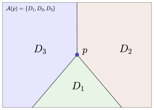
Figure 13. Sketch of a Julia pre-critical boundary point $p\in\mathbb{C}$, with $\mathcal{A}(f)$ finite.

Case 2 (Extended dreadlock). In this case, $w:=\widehat{f}(p)\in\mathbb{C}$ is the landing point of the dreadlock $G_{\underline{s}^{i}}$ used for the definition of the extended dreadlock $G_{\underline{s}^{i}}[a_{i}]$ that lands at the singular value $a_{i}\in S(f)\cap\mathcal{F}(f)$.

Recall that we have chosen the extended dreadlocks so as to avoid all further singular values, so $w$ is a regular value and hence $p\in\mathbb{C}$. We say that $p$ is a Julia regular boundary point.

Let $G_{\underline{t}}$ be the dreadlock that lands at $p$ so that $f(G_{\underline{t}})=G_{\underline{s}^{i}}$. By Corollary 6.10, there are unique partition sectors $I_{l},I_{r}\in\mathcal{I}$ such that $\underline{t}\in I_{l}^{+}\cap I_{r}^{-}$. We denote by $D_{l}(p),D_{r}(p)\in\mathcal{D}$ the corresponding partition sectors in the dynamic plane; see Figure 14 for an illustration.

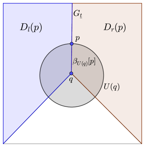
Figure 14. Sketch of a Julia regular boundary point $p$ (the shaded disk denotes the Fatou component that contains a point $q$ with $f(q)=a_{i}$).

We introduce the boundary symbol $\binom{D_{l}(z)}{D_{r}(z)}$ and call it a Julia regular boundary symbol. We call the point $p$ a Julia regular boundary point.

The introduction of these boundary symbols allows us to unambiguously define itineraries for all (pre-)periodic points in the extended Julia set.

Definition 7.1 (Itineraries of boundary points).

Let $p\in\mathcal{J}(\widehat{f})$ be (pre-)periodic, and write $p_{i}:=\widehat{f}^{\circ i}(p)$. We define the itinerary

$$\operatorname{It}(p\leavevmode\nobreak\ |\leavevmode\nobreak\ \widehat{\mathcal{D}}):=\operatorname{It}(p\leavevmode\nobreak\ |\leavevmode\nobreak\ \mathcal{D}):=\mathtt{\underline{u}}=\mathtt{u_{0}u_{1}\ldots}$$

of $p$ w.r.t. $\mathcal{D}$ as the sequence of partition sectors and boundary symbols defined via

$$\mathtt{u_{i}}:=\begin{cases}D_{i}\leavevmode\nobreak\ \leavevmode\nobreak\ \leavevmode\nobreak\ \text{if}\leavevmode\nobreak\ p_{i}\in\widehat{D_{i}},\\ \star_{\mathcal{A}(p_{i})}\leavevmode\nobreak\ \leavevmode\nobreak\ \leavevmode\nobreak\ \text{if}\leavevmode\nobreak\ p_{i}\in\partial\widehat{\mathcal{D}}\leavevmode\nobreak\ \text{and}\leavevmode\nobreak\ p_{i}\leavevmode\nobreak\ \text{is Julia pre-critical},\\ \binom{D_{l}(p_{i})}{D_{r}(p_{i})}\leavevmode\nobreak\ \leavevmode\nobreak\ \leavevmode\nobreak\ \text{if}\leavevmode\nobreak\ p_{i}\in\partial\widehat{\mathcal{D}}\leavevmode\nobreak\ \text{and}\leavevmode\nobreak\ p_{i}\leavevmode\nobreak\ \text{is Julia regular}.\end{cases}$$

The itinerary $\operatorname{It}(p\leavevmode\nobreak\ |\leavevmode\nobreak\ \mathcal{D})$ can contain boundary points of only one of the two kinds. Indeed, if $\operatorname{It}(p\leavevmode\nobreak\ |\leavevmode\nobreak\ \mathcal{D})$ contains a Julia pre-critical boundary symbol, then we have $\widehat{f}^{\circ n}(p)=a$ for some $n\geq 1$ and some $a\in S(f)$. If $\operatorname{It}(p\leavevmode\nobreak\ |\leavevmode\nobreak\ \mathcal{D})$ contains a Julia regular boundary symbol, then we have $\widehat{f}^{\circ n}(p)\notin S(f)$ for all $n\geq 0$. So the two cases are mutually exclusive.

In a way, points on the partition boundary realize several (pre-)periodic itineraries simultaneously. For example, if $a_{i}\in S(f)\cap\mathcal{F}(f)$ is a fixed point and $p=L(\underline{s}^{i})$, where $\underline{s}^{i}$ is the address from Definition 6.1, then there are sectors $D_{r}:=D_{r}(p)\in\mathcal{D}$ to the right of $G_{\underline{s}^{i}}[a_{i}]$ and $D_{l}:=D_{l}(p)$ to the left of $G_{\underline{s}^{i}}[a_{i}]$ (when standing at $a_{i}$ looking in the direction of the internal ray part of $G_{\underline{s}^{i}}[a_{i}]$) as described above (see also Figure 14). It turns out that, in this case, there is no periodic point of itinerary $D_{r}D_{r}D_{r}\ldots$ and, likewise, no periodic point of itinerary $D_{l}D_{l}D_{l}\ldots$ (this is easy to prove using a standard hyperbolic contraction argument for the backwards iteration, see Proposition 8.6). So one can say that the there is a point $p$ on the boundary of these sectors that realizes both of these itineraries at the same time.

In the following, we define adjacency relations to describe which (pre-)periodic sequences of partition sectors are realized by boundary points.

Definition 7.2 (Adjacent itineraries).

Let $\mathtt{\underline{u}}=(D_{i})_{i=0}^{\infty}$ be a sequence of partition sectors $D_{i}\in\mathcal{D}$. Let $p\in\mathcal{J}(\widehat{f})$ be (pre-)periodic. We call $\operatorname{It}(p\leavevmode\nobreak\ |\leavevmode\nobreak\ \mathcal{D})$ adjacent to $\mathtt{\underline{u}}$ if one of the following is true:

1. We have $\operatorname{It}(p\leavevmode\nobreak\ |\leavevmode\nobreak\ \mathcal{D})=\mathtt{\underline{u}}$. Then $\operatorname{It}(p\leavevmode\nobreak\ |\leavevmode\nobreak\ \mathcal{D})$ is free of boundary symbols.

2. The itinerary $\operatorname{It}(p\leavevmode\nobreak\ |\leavevmode\nobreak\ \mathcal{D})=\mathtt{\underline{t}}=\mathtt{t_{1}t_{2}\ldots}$ contains Julia pre-critical boundary symbols. For all boundary symbols $\mathtt{t}_{i}=\star_{\mathcal{A}_{i}}$, we have $D_{i}\in\mathcal{A}_{i}$. Otherwise, we have $\mathtt{t_{i}}=D_{i}$.

3. The itinerary $\operatorname{It}(p\leavevmode\nobreak\ |\leavevmode\nobreak\ \mathcal{D})=\mathtt{\underline{t}}=\mathtt{t_{1}t_{2}\ldots}$ contains Julia regular boundary symbols. For all boundary symbols $\mathtt{t}_{i}=\binom{D_{l}^{i}}{D_{r}^{i}}$, we have $D_{l}^{i}=D_{i}$. Otherwise, we have $\mathtt{t_{i}}=D_{i}$.

4. The itinerary $\operatorname{It}(p\leavevmode\nobreak\ |\leavevmode\nobreak\ \mathcal{D})=\mathtt{\underline{t}}=\mathtt{t_{1}t_{2}\ldots}$ contains Julia regular boundary symbols. For all boundary symbols $\mathtt{t}_{i}=\binom{D_{l}^{i}}{D_{r}^{i}}$, we have $D_{r}^{i}=D_{i}$. Otherwise, we have $\mathtt{t_{i}}=D_{i}$.

It should be clear that every (pre-)periodic point in the Julia set has an itinerary that is adjacent to one without boundary symbols

Let us now turn attention to the case of (pre-)periodic points in the Fatou set and explain how they fit into the context of dynamic partitions. For a post-critically finite polynomial, there exists an orbifold metric in a neighborhood of its Julia set w.r.t. which the map is expanding [Mil06, Section 19]. This expansivity is the reason why dynamic partitions of post-critically finite polynomials have a Markov type property (at least under certain assumptions on the dynamic rays used to define the partition): up to an adjacency relation similar to the one defined above, every abstract itinerary is realized by one and only one point in the Julia set. Because of this property, dynamic partitions should be viewed as partitions of the Julia set of the map.

We may still define itineraries of (pre-)periodic Fatou points as sequences that are, by definition, neither equal nor adjacent to any of the itineraries realized by points in the Julia set. To do this, we introduce another kind of boundary symbol. For a (pre-)periodic point $p\in\mathcal{F}(\widehat{f})$ that lies on the partition boundary, we denote by $\mathcal{A}(p)\subset\mathcal{D}$ — just as in the Julia pre-crictial case — the set of partition sectors $D\in\mathcal{A}(p)$ for which $p\in\partial_{\mathbb{C}_{{f}^{{{\infty}}}}}D$. We introduce the boundary symbol $\diamond_{\mathcal{A}(p)}$ and call it a Fatou boundary symbol.

Definition 7.3 (Itineraries of points in the Fatou set).

Let $p\in\mathcal{F}(\widehat{f})$ be (pre-)periodic and write $p_{i}=\widehat{f}^{\circ i}(p)$. We define the itinerary

$$\operatorname{It}(p\leavevmode\nobreak\ |\leavevmode\nobreak\ \widehat{\mathcal{D}}):=\operatorname{It}(p\leavevmode\nobreak\ |\leavevmode\nobreak\ \mathcal{D}):=\mathtt{\underline{u}}=\mathtt{u_{0}u_{1}}\ldots$$

of $p$ w.r.t. $\mathcal{D}$ to be the sequence of partition sectors and Fatou boundary symbols defined via

$$\mathtt{u_{i}}:=\begin{cases}D_{i}\leavevmode\nobreak\ \leavevmode\nobreak\ \leavevmode\nobreak\ \text{if}\leavevmode\nobreak\ p_{i}\in\widehat{D_{i}},\\ \diamond_{\mathcal{A}(p_{i})}\leavevmode\nobreak\ \leavevmode\nobreak\ \leavevmode\nobreak\ \text{if}\leavevmode\nobreak\ p_{i}\in\partial_{\mathbb{C}_{{f}^{{{\infty}}}}}\mathcal{D}.\end{cases}$$

We also need to define itineraries and the adjacency relation on the level of external addresses.

Definition 7.4 (Combinatorial itineraries).

Let $\mathcal{I}$ be a dynamic partition of $\mathbf{S}$. For every external address $\underline{t}\in\partial\mathcal{I}$ there exist unique partition sectors $I_{r}(\underline{t}),I_{l}(\underline{t})\in\mathcal{I}$ such that $\underline{t}\in I_{r}(\underline{t})^{-}\cap I_{l}(\underline{t})^{+}$ by Corollary 6.10.

We define the itinerary $\operatorname{It}(\underline{t}\leavevmode\nobreak\ |\leavevmode\nobreak\ \mathcal{I})=\mathtt{\underline{u}}=\mathtt{u_{0}u_{1}\ldots}$ of $\underline{t}$ w.r.t. $\mathcal{I}$ as the sequence defined via

$$\mathtt{u_{i}}=\begin{cases}I\leavevmode\nobreak\ \leavevmode\nobreak\ \leavevmode\nobreak\ \text{if}\leavevmode\nobreak\ \sigma^{\circ i}(\underline{t})\in I,\\ \binom{I_{l}(\underline{t})}{I_{r}(\underline{t})}\leavevmode\nobreak\ \leavevmode\nobreak\ \leavevmode\nobreak\ \text{if}\leavevmode\nobreak\ \underline{t}\in\partial\mathcal{I}.\end{cases}$$

Adding consistently either the left- or the right-sided boundary addresses to the partition sectors, we obtain two full partitions of the space of external addresses, i.e., we have $\mathbf{S}=\mathop{\vphantom{\bigcup}\mathchoice{\leavevmode\vtop{\halign{\hfil$\m@th\displaystyle#$\hfil\cr\bigcup\cr\cdot\crcr}}}{\leavevmode\vtop{\halign{\hfil$\m@th\textstyle#$\hfil\cr\bigcup\cr\cdot\crcr}}}{\leavevmode\vtop{\halign{\hfil$\m@th\scriptstyle#$\hfil\cr\bigcup\cr\cdot\crcr}}}{\leavevmode\vtop{\halign{\hfil$\m@th\scriptscriptstyle#$\hfil\cr\bigcup\cr\cdot\crcr}}}}\displaylimits_{I\in\mathcal{I}}I^{-}$ and $\mathbf{S}=\mathop{\vphantom{\bigcup}\mathchoice{\leavevmode\vtop{\halign{\hfil$\m@th\displaystyle#$\hfil\cr\bigcup\cr\cdot\crcr}}}{\leavevmode\vtop{\halign{\hfil$\m@th\textstyle#$\hfil\cr\bigcup\cr\cdot\crcr}}}{\leavevmode\vtop{\halign{\hfil$\m@th\scriptstyle#$\hfil\cr\bigcup\cr\cdot\crcr}}}{\leavevmode\vtop{\halign{\hfil$\m@th\scriptscriptstyle#$\hfil\cr\bigcup\cr\cdot\crcr}}}}\displaylimits_{I\in\mathcal{I}}I^{+}$. Therefore, it makes sense to distinguish between left-sided and right-sided itineraries that contain boundary symbols.

Definition 7.5 (Left- and right-sided itineraries).

Let $\underline{s}$ be an external address and let $\mathcal{I}$ be a dynamic partition. For every $j\geq 0$, there exists a unique partition sector $I_{j}^{l}$ such that $\sigma^{\circ j}(\underline{s})\in(I_{j}^{l})^{-}$. The sequence

$$\operatorname{It}^{-}(\underline{s}\leavevmode\nobreak\ |\leavevmode\nobreak\ \mathcal{I}):=(I_{j}^{l})_{j=0}^{\infty}=I_{0}^{l}I_{1}^{l}\ldots$$

is called the left-sided itinerary of $\underline{s}$ w.r.t. $\mathcal{I}$. In the same manner, we define the right-sided itinerary of $\underline{s}$ w.r.t. $\mathcal{I}$ as the sequence

$$\operatorname{It}^{+}(\underline{s}\leavevmode\nobreak\ |\leavevmode\nobreak\ \mathcal{I}):=(I_{j}^{r})_{j=0}^{\infty}=I_{0}^{r}I_{1}^{r}\ldots$$

where we have $\sigma^{\circ j}(\underline{s})\in(I_{j}^{r})^{+}$. We call the itinerary $\operatorname{It}(\underline{s}\leavevmode\nobreak\ |\leavevmode\nobreak\ \mathcal{I})$ adjacent to $\mathtt{\underline{u}}\in\mathcal{I}^{\mathbb{N}}$ if $\operatorname{It}^{-}(\underline{s}\leavevmode\nobreak\ |\leavevmode\nobreak\ \mathcal{I})=\mathtt{\underline{u}}$ or $\operatorname{It}^{+}(\underline{s}\leavevmode\nobreak\ |\leavevmode\nobreak\ \mathcal{I})=\mathtt{\underline{u}}$.

Let us describe the relationship between the adjacency relations on the space of external addresses and on the plane (at least in one direction).

Lemma 7.6 (Adjacent itineraries).

Let $\underline{s}\in\mathbf{S}$ be (pre-)periodic and let $(I_{j})_{j=0}^{\infty}$ be a sequence of partition sectors. If $\operatorname{It}(\underline{s}\leavevmode\nobreak\ |\leavevmode\nobreak\ \mathcal{I})$ is adjacent to $(I_{j})_{j=0}^{\infty}$, then $\operatorname{It}(L(\underline{s})\leavevmode\nobreak\ |\leavevmode\nobreak\ \mathcal{D})$ is adjacent to $(D(I_{j}))_{j=0}^{\infty}$.

Proof.

Let $p:=L(\underline{s})$ be the landing point of $G_{\underline{s}}$, and set $p_{j}:=\widehat{f}^{\circ j}(p)$ for $j\geq 0$. If the forward orbit of $p$ does not intersect the partition boundary, the statement of the lemma follows from Proposition 6.7. Otherwise, we distinguish whether the forward orbit of $p$ contains Julia pre-critical or Julia regular boundary points. In both cases, we only proof the lemma for left-sided itineraries, i.e., we assume that $\operatorname{It}^{-}(\underline{s}\leavevmode\nobreak\ |\leavevmode\nobreak\ \mathcal{I})=(I_{j})_{j=0}^{\infty}$. For right-sided itineraries, the proof works in complete analogy.

Assume that $p$ contains Julia pre-critical points on its forward orbit, and choose $k\geq 0$ such that $p_{k}\in\partial\widehat{\mathcal{D}}$. By Corollary 6.9, we have $p_{k}\in\operatorname{cl}_{\mathbb{C}_{{f}^{{{\infty}}}}}(D(I_{k}))$. Therefore, $\operatorname{It}(p\leavevmode\nobreak\ |\leavevmode\nobreak\ \mathcal{D})$ is adjacent to $(D(I_{j}))_{j=0}^{\infty}$ by Property (2) of Definition 7.2.

Next, assume that $p$ contains Julia regular boundary points on its forward orbit, and choose $k\geq 0$ such that $p_{k}\in\partial\widehat{\mathcal{D}}$. It follows from the definition of left and right sectors that $D(I_{k})=D_{r}(p_{k})$. Therefore, $\operatorname{It}(p\leavevmode\nobreak\ |\leavevmode\nobreak\ \mathcal{D})$ is adjacent to $(D(I_{j}))_{j=0}^{\infty}$ by Property (3) of Definition 7.2. ∎

8. The Landing Equivalence Relation

In order to obtain a nice combinatorial description of the landing equivalence relation, we use dynamic partitions that satisfy some additional properties. One of these properties concerns the choice of extended dreadlocks for singular values in the Fatou set.

Definition 8.1 (Minimal extended dreadlock).

Let $p\in\mathbb{C}_{{f}^{{{\infty}}}}$ be the center of a Fatou component, let $m$ be the preperiod of $p$, and let $n$ be the period of $p$. An extended dreadlock $G_{\underline{s}}[p]$ is called minimal if $\widehat{f}^{\circ m+n}(G_{\underline{s}}[p])=\widehat{f}^{\circ m}(G_{\underline{s}}[p])$.

We want to choose for every $a\in S(f)\cap\mathcal{J}(f)$ a dreadlock that lands at $a$ and for every $a\in S(f)\cap\mathcal{F}(f)$ a minimal extended dreadlock that lands at $a$ such that the chosen (extended) dreadlocks are pairwise disjoint. This is not always possible, as for example the only fixed point on the boundary of a degree $2$ fixed Fatou component might itself be a singular value. But if this is possible, and some additional properties hold, we are able to define a dynamic partition with particularly nice properties.

Definition 8.2 (Simple dynamic partition).

Let $f$ be a psf entire function, and let $\mathcal{D}=\mathcal{D}(\{G_{\underline{s}^{i}}[a_{i}]\})$ be a dynamic partition for $f$. We call $\mathcal{D}$ a simple dynamic partition if the following properties are satisfied.

1. All periodic post-singular points are fixed, and all dreadlocks that land at periodic post-singular points in $\mathcal{J}(f)$ are fixed.

2. For every $a_{i}\in S(f)\cap\mathcal{F}(f)$, the dreadlock $G_{\underline{s}^{i}}[a_{i}]$ is minimal.

3. We have $\bigcup_{i\in\{1,\ldots,n\}}\bigcup_{j\geq 0}f^{\circ j}(G_{\underline{s}^{i}}[a_{i}])=\mathop{\vphantom{\bigcup}\mathchoice{\leavevmode\vtop{\halign{\hfil$\m@th\displaystyle#$\hfil\cr\bigcup\cr\cdot\crcr}}}{\leavevmode\vtop{\halign{\hfil$\m@th\textstyle#$\hfil\cr\bigcup\cr\cdot\crcr}}}{\leavevmode\vtop{\halign{\hfil$\m@th\scriptstyle#$\hfil\cr\bigcup\cr\cdot\crcr}}}{\leavevmode\vtop{\halign{\hfil$\m@th\scriptscriptstyle#$\hfil\cr\bigcup\cr\cdot\crcr}}}}\displaylimits_{p\in P(f)}G_{\underline{s}(p)}[p]$ for certain external addresses $\underline{s}(p)\in\mathbf{S}$.

It turns out that every psf entire function has an iterate that admits a simple dynamic partition.

Proposition 8.3 (Existence of simple dynamic partitions).

Let $f$ be a psf entire function. There exists an $n\geq 1$ such that $f^{\circ n}$ admits a simple dynamic partition.

Proof.

By passing to a suitable iterate, we can make sure that Property (1) is satisfied. This property remains satisfied when passing to an iterate once again. Possibly after passing to an iterate for a second time, we are able to choose for every fixed $p\in P(f)\cap\mathcal{F}(f)$ a fixed internal ray $\beta_{U(p)}[q(p)]$ such that the landing points $q(p)$ are distinct, are not contained in $P(f)$, and all dreadlocks that land at any of the $q(p)$ are fixed. It follows that there exists for every fixed $p\in P(f)\cap\mathcal{F}(f)$ a minimal left-supporting dreadlock $G_{\underline{s}(p)}[p]$ and for every fixed $p\in P(f)\cap\mathcal{J}(f)$ a dreadlock $G_{\underline{s}(p)}$ that lands at $p$ such that the chosen (extended) dreadlocks are pairwise disjoint.

Assume that for a given $i\geq 0$ we have already chosen an (extended) dreadlock for every $p\in P(f)$ such that $f^{\circ i}(p)$ is periodic (and hence fixed). Let $p\in P(f)$ be a point that is mapped to a periodic point after $i+1$ iterations, and set $q:=f(p)$. Let $G_{\underline{s}(q)}[q]$ be the extended dreadlock chosen for $q$. If $p$ has local mapping degree $d\geq 1$, then there are $d$ ways to lift $G_{\underline{s}(q)}[q]$ to an (extended) dreadlock that lands at $p$. It does not matter which lift we choose, so let $G_{\underline{s}(p)}[p]$ be one of those lifts. By construction, the resulting dreadlocks $G_{\underline{s}(p)}[p]$ are still pairwise disjoint. We continue inductively until we have chosen an (extended) dreadlock for every post-singular point. In particular, we have chosen an (extended) dreadlock for every singular value, denote these dreadlocks by $G_{\underline{s}^{i}}[a_{i}]$. Properties (2) and (3) are satisfied by construction. ∎

Our first important result on simple dynamic partitions is that for every(pre-)periodic sequence $(D_{i})_{i=0}^{\infty}$ of partition sectors there is at most one(pre-)periodic point $p\in\mathcal{J}(\widehat{f})$ for which $\operatorname{It}(p\leavevmode\nobreak\ |\leavevmode\nobreak\ \mathcal{D})$ is adjacent to $(D_{i})_{i=0}^{\infty}$. The following two lemmata are needed for the proof.

Lemma 8.4 (Fixed boundary points).

Let $\mathcal{D}$ be a simple dynamic partition, and let $p\in\partial\mathcal{D}\cap\mathcal{J}(f)$ be periodic and hence fixed. Let $\mathtt{\underline{u}}\in\mathcal{D}^{\mathbb{N}}$ be adjacent to $\operatorname{It}(p\leavevmode\nobreak\ |\leavevmode\nobreak\ \mathcal{D})$. Then $\mathtt{\underline{u}}=DDD\ldots$ for some $D\in\mathcal{D}$.

Let $g:=f^{-1}\colon\mathbb{C}\setminus\bigcup_{i}\overline{G_{\underline{s}^{i}}[a_{i}]}\to D$ be the inverse branch mapping the complement of the (extended) dreadlocks used for the definition of $\mathcal{D}$ onto $D$. Then, for every neighborhood $U$ of $p$, there exists a point $b_{0}\in U\setminus\bigcup_{i}\overline{G_{\underline{s}^{i}}[a_{i}]}$ such that the sequence $(b_{i})_{i=0}^{\infty}$ defined via $b_{i}:=g^{\circ i}(b_{0})$ is well-defined and satisfies $b_{i}\to p$.

Proof.

We distinguish two cases. First, assume that $p=a_{i}\in S(f)$. Let $U_{i}\supset G_{\underline{s}^{i}}[a_{i}]$ be simply connected such that $U_{i}\cap G_{\underline{s}^{j}}[a_{j}]=\emptyset$ for $j\neq i$. Let $V_{i}$ be the connected component of $f^{-1}(U_{i})$ containing $p$. Then $\partial\mathcal{D}\cap V_{i}=G_{\underline{s}^{i}}[a_{i}]$, and the complement $V:=V_{i}\setminus G_{\underline{s}^{i}}[a_{i}]$ is simply connected by Theorem 5.7. It follows that $V\subset D$ for some partition sector $D\in\mathcal{D}$. This implies that $D$ is the only partition sector for which $p\in\partial_{\mathbb{C}_{{f}^{{{\infty}}}}}D$. By Definition 7.2, the only itinerary adjacent to $\operatorname{It}(p\leavevmode\nobreak\ |\leavevmode\nobreak\ \mathcal{D})$ is $\mathtt{\underline{u}}=DDD\ldots$.

Let $U\subset V_{i}$ be a linearizing neighborhood of $p$, and let $b_{0}\in U\cap V$. Let $f_{D}^{-1}\colon\mathbb{C}\setminus\bigcup_{i}\overline{G_{\underline{s}^{i}}[a_{i}]}\to D$ be the unique inverse branch of $f$ with the prescribed domain and co-domain. Inductively, we define $b_{i}:=f_{D}^{-1}(b_{i-1})$. By the preceding paragraph, we have $b_{i}\in V\subset D$ for all $i\geq 0$. As $U$ is a linearizing neighborhood of $p$, it follows that $\lim_{i\to\infty}b_{i}=p$.

The second case is that $p\notin S(f)$, so $p\in G_{\underline{s}^{i}}[a_{i}]$ for some fixed $a_{i}\in S(f)\cap\mathcal{F}(f)$. It follows from Definition 7.2 that either $\mathtt{\underline{u}}=D_{l}(p)D_{l}(p)\ldots$ or $\mathtt{\underline{u}}=D_{r}(p)D_{r}(p)\ldots$. Assume w.l.o.g. that $\mathtt{\underline{u}}=D_{l}(p)D_{l}(p)\ldots$; the second case works analogously. Let $U$ be a linearizing neighborhood for $p$. There exists a point $b_{0}\in U\cap D_{l}(p)$ that can be connected to a point $w\in\beta_{U(a_{i})}[p]$ via an arc $\gamma\colon[0,1]\to\mathbb{C}$ satisfying $\gamma([0,1))\subset D_{l}(p)\cap U$. Inductively, we define $b_{i}:=f_{D_{l}(p)}^{-1}(b_{i-1})$. Let $w^{\prime}$ be the unique preimage of $w$ on $\beta_{U(a_{i})}[p]$. The unique lift of $\gamma$ starting at $w^{\prime}$ ends at $b_{1}$, as conformal maps are orientation-preserving. It follows inductively that $b_{i}\in U$ for all $i\geq 0$ and therefore $b_{i}\to p$. ∎

Lemma 8.5 (Preimage itineraries).

Let $\mathtt{\underline{u}}=(D_{i})_{i=0}^{\infty}$ be a sequence of itinerary domains, and let $p\in\mathcal{J}(\widehat{f})$ be a (pre-)periodic point whose itinerary $\operatorname{It}(p\leavevmode\nobreak\ |\leavevmode\nobreak\ \mathcal{D})$ is adjacent to $\mathtt{\underline{u}}$. Let $D\in\mathcal{D}$ be a partition sector. Then there exists one and only one $q\in\widehat{f}^{-1}(p)$ such that $\operatorname{It}(q\leavevmode\nobreak\ |\leavevmode\nobreak\ \mathcal{D})$ is adjacent to $D\mathtt{\underline{u}}$.

Proof.

First, assume that $p\in\mathbb{C}_{{f}^{{{\infty}}}}\setminus\bigcup_{i\in\{1,\ldots,n\}}\operatorname{cl}_{\mathbb{C}_{{f}^{{{\infty}}}}}(G_{\underline{s}^{i}}[a_{i}])$. Then every preimage of $p$ is contained in some partition sector and every partition sector contains precisely one preimage of $p$ by Lemma 6.3. Therefore, the unique preimage $q\in\widehat{f}^{-1}(p)\cap D$ is the only point for which $\operatorname{It}(q\leavevmode\nobreak\ |\leavevmode\nobreak\ \mathcal{D})$ is adjacent to $D\mathtt{\underline{u}}$.

Else, we have $p\in\overline{G_{\underline{s}^{i}}[a_{i}]}$ for some $i\in\{1,\ldots,n\}$. If $p\in S(f)$, then there exists a unique preimage $q\in\widehat{f}^{-1}(p)$ satisfying $q\in\partial_{\mathbb{C}_{{f}^{{{\infty}}}}}D$ by Lemma 6.6. By the definition of adjacency, this implies that $q$ is the only preimage of $p$ whose itinerary is adjacent to $D\mathtt{\underline{u}}$.

Otherwise, we have $p\notin S(f)$ and $p=L(\underline{s}^{i})$. By Proposition 6.8 and the definition of right and left sectors, there are unique preimages $q_{l},q_{r}\in f^{-1}(p)$ such that $D_{l}(q_{l})=D$ and $D_{r}(q_{r})=D$. If $\operatorname{It}(p\leavevmode\nobreak\ |\leavevmode\nobreak\ \mathcal{D})$ is related to $\mathtt{\underline{u}}$ via case (3) of Definition 7.2, then $q_{l}$ is the only preimage of $p$ whose itinerary is adjacent to $D\mathtt{\underline{u}}$. If instead $\operatorname{It}(p\leavevmode\nobreak\ |\leavevmode\nobreak\ \mathcal{D})$ is related to $\mathtt{\underline{u}}$ via case (4) of Definition 7.2, then $q_{r}$ is the only preimage of $p$ whose itinerary is adjacent to $D\mathtt{\underline{u}}$. ∎

We are now in the position to prove that a (pre-)periodic itinerary is realized by at most one (pre-)periodic point. The result is a generalization of [SZ03b, Proposition 4.4], and the underlying proof strategy is taken from there.

Proposition 8.6 (Unique itineraries).

Let $\mathcal{D}$ be a simple dynamic partition, and let $\mathtt{\underline{u}}=E_{0}\ldots E_{k-1}\overline{D_{0}D_{1}\ldots D_{m-1}}$ be a (pre-)periodic sequence of partition sectors. Let $p,q\in\mathcal{J}(\widehat{f})$ be (pre-)periodic points, and assume that $\operatorname{It}(p\leavevmode\nobreak\ |\leavevmode\nobreak\ \mathcal{D})$ and $\operatorname{It}(q\leavevmode\nobreak\ |\leavevmode\nobreak\ \mathcal{D})$ are both adjacent to $\mathtt{\underline{u}}$. Then $p=q$.

Proof.

Let $G_{\underline{s}^{1}}[a_{1}],\ldots,G_{\underline{s}^{n}}[a_{n}]$ be the (extended) dreadlocks from Definition 8.2 that land at the singular values of $f$. We set

$$W:=\mathbb{C}\setminus\bigcup_{i=1}^{n}\bigcup_{m\geq 0}f^{\circ m}(\overline{G_{\underline{s}^{i}}[a_{i}]}).$$

By Property (3) of Definition 8.2, the complement $\mathbb{C}\setminus W$ consists of finitely many pairwise disjoint (extended) dreadlocks. By Proposition 5.4 and Proposition 5.15, none of these (extended) dreadlocks separates the plane. Hence, the complement $W$ is simply connected by Theorem 5.7. The domain $W$ is backward invariant and satisfies $W\subset\mathbb{C}\setminus\bigcup_{i=1}^{n}\overline{G_{\underline{s}^{i}}[a_{i}]}$. Hence, for every itinerary domain $D$ the unique branch $f^{-1}\colon\mathbb{C}\setminus\bigcup_{i=1}^{n}\overline{G_{\underline{s}^{i}}[a_{i}]}\to D$ of the inverse of $f$ restricts to a branch $f_{D}^{-1}\colon W\to D$. We set $W_{D}:=f_{D}^{-1}(W)\subset W$.

Assume for now that $\mathtt{\underline{u}}=\overline{D_{0}\ldots D_{m-1}}$ is periodic, and $p$ and $q$ are periodic. Assume by contradiction that $p\neq q$. In addition, assume that $p,q\in W$. Note that this implies $f^{\circ i}(p),f^{\circ i}(q)\in W$ for all $i\geq 0$, and therefore $\operatorname{It}(p\leavevmode\nobreak\ |\leavevmode\nobreak\ \mathcal{D})=\operatorname{It}(q\leavevmode\nobreak\ |\leavevmode\nobreak\ \mathcal{D})=\mathtt{\underline{u}}$. Choose $m\in\mathbb{N}$ such that $f^{\circ m}(p)=p$ as well as $f^{\circ m}(q)=q$, and write $p_{i}:=f^{\circ i}(p)$ as well as $q_{i}:=f^{\circ i}(q)$. We have $p_{i}=f_{D_{i}}^{-1}(p_{i+1})$ as well as $q_{i}=f_{D_{i}}^{-1}(q_{i+1})$. Setting $g:=f_{D_{0}}^{-1}\circ f_{D_{1}}^{-1}\circ\ldots\circ f_{D_{m-1}}^{-1}\colon W\to W$, we obtain a univalent self-map of $W$ satisfying $g(p)=p$ and $g(q)=q$. If $p$ and $q$ were distinct, this would imply $g=\text{id}$. Hence, we have $p=q$.

In general, both $p$ and $q$ might be contained in $\partial W$. Assume for now that $p\in\partial W$ and $q\in W$. Then Property (1) of Definition 8.2 implies that $p$ is fixed and so is every itinerary adjacent to $\operatorname{It}(p\leavevmode\nobreak\ |\leavevmode\nobreak\ \mathcal{D})$ by Lemma 8.4. Hence, we have $\mathtt{\underline{u}}=DDD\ldots$ for some itinerary domain $D\in\mathcal{D}$. By Lemma 8.4, there exists a point $b_{0}\in W$ such that the sequence $(b_{i})_{i=0}^{\infty}$ defined via $b_{i+1}:=f_{D}^{-1}(b_{i})$ converges to $p$. Assume that $q\in W$, and let $\alpha_{0}\colon[0,1]\to W$ be a smooth arc of finite length w.r.t. the hyperbolic metric on $W$ that connects $b_{0}=\alpha_{0}(0)$ to $q=\alpha_{0}(1)$. By the preceding paragraph, we have $f_{D}^{-1}(q)=q$. Hence, the lift $\alpha_{1}:=f_{D}^{-1}\circ\alpha_{0}$ connects $b_{1}$ to $q$, and it satisfies

$$l_{W}(\alpha_{1})<l_{f_{D}^{-1}(W)}(\alpha_{1})=l_{W}(\alpha_{0}),$$

where the first inequality follows from the comparison principle, and the second equality follows from Pick’s Theorem. Inductively, we define $\alpha_{i+1}:=f_{D}^{-1}\circ\alpha_{i}$. As we have $l_{W}(\alpha_{i})<l_{W}(\alpha_{0})$ and $\alpha_{i}(0)=b_{i}\to p\in\partial W$ for $i\to\infty$, the Euclidean lengths of the $\alpha_{i}$ tend to $0$ contradicting our assumption that $p$ and $q$ are distinct.

An analogous argument works if both $p$ and $q$ are contained in $\partial W$. In this case, we also have to take a point $\tilde{b}_{0}$ as in Lemma 8.4 for $q$ and connect $b_{0}$ to $\tilde{b}_{0}$ via an arc $\alpha_{0}$ of finite hyperbolic length.

Let us now prove the full statement of the lemma. We set $p_{i}:=\widehat{f}^{\circ i}(p)$ and $q_{i}:=\widehat{f}^{\circ i}(q)$. Choose $n\geq 0$ such that $p_{n}$ and $q_{n}$ are both periodic. Then $\mathtt{\underline{\tilde{u}}}:=\sigma^{\circ n}(\mathtt{\underline{u}})$ is also periodic, and both $\operatorname{It}(p_{n}\leavevmode\nobreak\ |\leavevmode\nobreak\ \mathcal{D})$ and $\operatorname{It}(q_{n}\leavevmode\nobreak\ |\leavevmode\nobreak\ \mathcal{D})$ are adjacent to $\mathtt{\underline{\tilde{u}}}$. By the periodic case proved above, we have $p_{n}=q_{n}$. Applying Lemma 8.5 inductively for $n$ times, we obtain $p=q$. ∎

We have thus shown that every (pre-)periodic itinerary is realized by at most one (pre-)periodic point. The next step is to show that every (pre-)periodic itinerary is, in fact, realized.

Lemma 8.7 (Pullbacks of intervals).

Let $I,I^{\prime}\in\mathcal{I}$ be partition sectors, and let $J\subset I$ be an interval. If $\underline{s}^{i}\notin J$ for all $i$, then $J^{\prime}:=\sigma^{-1}(J)\cap I^{\prime}$ is an interval of the form $J^{\prime}=\{F\underline{t}\leavevmode\nobreak\ |\leavevmode\nobreak\ \underline{t}\in J\}$ for some fundamental domain $F$.

Proof.

For the proof, we are going to use concepts introduced in subsubsections 3.2.1 and 3.2.2. In particular, we are going to talk about the successor $F_{p}$ of a fundamental domain, the circle of addresses $\overline{\mathbf{S}}$, and the intermediate address $\alpha$ with its preimages $\alpha_{F_{p}}^{F}\in\sigma^{-1}(\alpha)$.

By the proof of Proposition 6.8, there are fundamental domains $F_{1},\ldots,F_{n}$ such that

$$I^{\prime}=((F_{1})_{p}\underline{s}^{n},F_{1}\underline{s}^{1})\mathbin{\mathchoice{\leavevmode\vtop{\halign{\hfil$\m@th\displaystyle#$\hfil\cr\cup\cr\cdot\crcr}}}{\leavevmode\vtop{\halign{\hfil$\m@th\textstyle#$\hfil\cr\cup\cr\cdot\crcr}}}{\leavevmode\vtop{\halign{\hfil$\m@th\scriptstyle#$\hfil\cr\cup\cr\cdot\crcr}}}{\leavevmode\vtop{\halign{\hfil$\m@th\scriptscriptstyle#$\hfil\cr\cup\cr\cdot\crcr}}}}(F_{2}\underline{s}^{1},F_{2}\underline{s}^{2})\mathbin{\mathchoice{\leavevmode\vtop{\halign{\hfil$\m@th\displaystyle#$\hfil\cr\cup\cr\cdot\crcr}}}{\leavevmode\vtop{\halign{\hfil$\m@th\textstyle#$\hfil\cr\cup\cr\cdot\crcr}}}{\leavevmode\vtop{\halign{\hfil$\m@th\scriptstyle#$\hfil\cr\cup\cr\cdot\crcr}}}{\leavevmode\vtop{\halign{\hfil$\m@th\scriptscriptstyle#$\hfil\cr\cup\cr\cdot\crcr}}}}\ldots\mathbin{\mathchoice{\leavevmode\vtop{\halign{\hfil$\m@th\displaystyle#$\hfil\cr\cup\cr\cdot\crcr}}}{\leavevmode\vtop{\halign{\hfil$\m@th\textstyle#$\hfil\cr\cup\cr\cdot\crcr}}}{\leavevmode\vtop{\halign{\hfil$\m@th\scriptstyle#$\hfil\cr\cup\cr\cdot\crcr}}}{\leavevmode\vtop{\halign{\hfil$\m@th\scriptscriptstyle#$\hfil\cr\cup\cr\cdot\crcr}}}}(F_{n}\underline{s}^{n},(F_{n})_{s}\underline{s}^{1}).$$

The restriction $\left.\sigma\right|_{I^{\prime}}$ is an order-preserving bijection onto $\mathbf{S}\setminus\{\underline{s}^{1},\ldots,\underline{s}^{n}\}$. As $\underline{s}^{i}\notin J$ for all $i$ by hypothesis, the preimage $J^{\prime}=\left.\sigma\right|_{I^{\prime}}^{-1}(J)$ is contained in one of the intervals above.

If $J^{\prime}\subset(F_{i}\underline{s}^{i-1},F_{i}\underline{s}^{i})$ for some $i\in\{2,\ldots,n-1\}$, the claim follows because all external addresses of the interval $(F_{i}\underline{s}^{i-1},F_{i}\underline{s}^{i})$ have first entry $F_{i}$. If instead $J^{\prime}\subset((F_{1})_{p}\underline{s}^{n},F_{1}\underline{s}^{1})$, the claim follows from the fact that $J\subset I$ for some partition sector $I$: we have $\alpha\notin\operatorname{cl}_{\overline{\mathbf{S}}}(J)$, so $J^{\prime}\cap\sigma^{-1}(\alpha)=\emptyset$. Hence, either $J^{\prime}\subset((F_{1})_{p}\underline{s}^{n},\alpha_{(F_{1})_{p}}^{F_{1}})\subset(F_{1})_{p}$ or $J^{\prime}\subset(\alpha_{(F_{1})_{p}}^{F_{1}},F_{1}\underline{s}^{1})\subset F_{1}$. The case $J^{\prime}\subset(F_{n}\underline{s}^{n},(F_{n})_{s}\underline{s}^{1})$ works analogously. ∎

Proposition 8.8 (Realized itineraries).

Let $\mathcal{I}$ be a (not necessarily simple) dynamic partition. Then, for every periodic sequence $\mathtt{\underline{u}}=\overline{I_{0}I_{1}\ldots I_{m-1}}$ of itinerary domains, there exists a periodic external address $\underline{s}\in\mathcal{S}$ such that either $\operatorname{It}^{+}(\underline{s}\leavevmode\nobreak\ |\leavevmode\nobreak\ \mathcal{I})=\mathtt{\underline{u}}$ or $\operatorname{It}^{-}(\underline{s}\leavevmode\nobreak\ |\leavevmode\nobreak\ \mathcal{I})=\mathtt{\underline{u}}$.

Proof.

The set

$$T:=\bigcup_{i\in\{1,\ldots,n\}}\bigcup_{j\geq 0}\{\sigma^{\circ j}(\underline{s}^{i})\}$$

is finite and forward invariant. By Proposition 6.8, we have

$$I_{0}\setminus T=J_{1}^{(0)}\mathbin{\mathchoice{\leavevmode\vtop{\halign{\hfil$\m@th\displaystyle#$\hfil\cr\cup\cr\cdot\crcr}}}{\leavevmode\vtop{\halign{\hfil$\m@th\textstyle#$\hfil\cr\cup\cr\cdot\crcr}}}{\leavevmode\vtop{\halign{\hfil$\m@th\scriptstyle#$\hfil\cr\cup\cr\cdot\crcr}}}{\leavevmode\vtop{\halign{\hfil$\m@th\scriptscriptstyle#$\hfil\cr\cup\cr\cdot\crcr}}}}\ldots\mathbin{\mathchoice{\leavevmode\vtop{\halign{\hfil$\m@th\displaystyle#$\hfil\cr\cup\cr\cdot\crcr}}}{\leavevmode\vtop{\halign{\hfil$\m@th\textstyle#$\hfil\cr\cup\cr\cdot\crcr}}}{\leavevmode\vtop{\halign{\hfil$\m@th\scriptstyle#$\hfil\cr\cup\cr\cdot\crcr}}}{\leavevmode\vtop{\halign{\hfil$\m@th\scriptscriptstyle#$\hfil\cr\cup\cr\cdot\crcr}}}}J_{N}^{(0)},$$

where the $J_{i}^{(0)}$ are open intervals in $\mathbf{S}$. Inductively, we define

$$J_{i}^{(l)}:=\sigma^{-1}(J_{i}^{(l-1)})\cap I_{\mathtt{u}_{-l}}.$$

As $\mathbf{S}\setminus T$ is backward invariant, we have $J_{i}^{(l)}\cap T=\emptyset$ for all $i$ and $l$. Hence, Lemma 8.7 implies that every $J_{i}^{(l)}$ is an open interval and the first $l$ entries are the same for all addresses in $J_{i}^{(l)}$.

After $m$ pullbacks, we are back at subintervals of our initial partition sector $I_{0}$. We define $\rho\colon\{1,\ldots,N\}\to\{1,\ldots,N\}$ via $J_{i}^{(m)}\subset J_{\rho(i)}^{(0)}$. Choose $n_{0}$ and $i_{0}$ such that $\rho^{\circ n_{0}}(i_{0})=i_{0}$, and set $J^{(l)}:=J_{i_{0}}^{(lmn_{0})}$. The $J^{(l)}$ form a nested sequence of intervals. By Lemma 8.7, there exist fundamental domains $F_{1},\ldots,F_{n_{1}}$ (where $n_{1}:=mn_{0}$) such that every external address in $J^{(l)}$ begins with $l$ times the sequence $F_{1}\ldots F_{n_{1}}$. Therefore, we have

$$\underline{s}:=\overline{F_{1}\ldots F_{n_{1}}}\in\bigcap_{l}\operatorname{cl}(J^{(l)}).$$

Either the left- or the right-sided itinerary of $\underline{s}$ (or both) equals $\mathtt{\underline{u}}$. ∎

Corollary 8.9 (Itineraries are uniquely realized).

Let $\mathtt{\underline{u}}\in\mathcal{D}^{\mathbb{N}}$ be (pre-)periodic. Then there exists a unique (pre-)periodic point $p\in\mathcal{J}(\widehat{f})$ such that $\operatorname{It}(p\leavevmode\nobreak\ |\leavevmode\nobreak\ \mathcal{D})$ is adjacent to $\mathtt{\underline{u}}$.

Proof.

Lemma 7.6 and Proposition 8.8 imply that there exists a (pre-)periodic point $p\in\mathcal{J}(\widehat{f})$ for which $\operatorname{It}(p\leavevmode\nobreak\ |\leavevmode\nobreak\ \mathcal{D})$ is adjacent to $\mathtt{\underline{u}}$. Proposition 8.6 says that this point is unique. ∎

This corollary does not imply that the map sending a (pre-)periodic itinerary $\mathtt{\underline{u}}$ to the unique (pre-)periodic point $p\in\mathbb{C}_{{f}^{{{\infty}}}}$ for which $\operatorname{It}(p\leavevmode\nobreak\ |\leavevmode\nobreak\ \mathcal{D})$ is adjacent to $\mathtt{\underline{u}}$ is a bijection. Indeed, this is never the case. As noted in the preceding section, we have $C(\widehat{f})\neq\emptyset$ for all post-singularly finite maps $f$. The existence of critical points implies that several (pre-)periodic itineraries correspond to the same (pre-)periodic point.

The remaining goal of this work is to describe the landing equivalence relation in terms of itineraries w.r.t. some simple dynamic partition. The following lemma will be useful for the proof of the periodic case.

Lemma 8.10.

Let $p\in\mathcal{J}(\widehat{f})\setminus C(\widehat{f})$ be (pre-)periodic. Then there exists a partition sector $I\in\mathcal{I}$ such that the set

$$\operatorname{Ad}(p):=\{\underline{s}\in\mathbf{S}\colon L(\underline{s})=p\}$$

satisfies $\operatorname{Ad}(p)\subset I^{-}$.

Proof.

First, assume that $p\notin\partial_{\mathbb{C}_{{f}^{{{\infty}}}}}\mathcal{D}$, so $p\in\widehat{D}$ (see Definition 6.2) for some $D\in\mathcal{D}$. All dreadlocks that land at $p$ are entirely contained in $\widehat{D}$, so $\operatorname{Ad}(p)\subset I(D)$ by Proposition 6.7.

If $p\in\partial_{\mathbb{C}_{{f}^{{{\infty}}}}}\mathcal{D}$ is a Julia critical boundary point, it follows from $p\notin C(\widehat{f})$ and Lemma 6.11 that there is a partition sector $I\in\mathcal{I}$ so that $\operatorname{Ad}(p)\subset I^{-}$.

If instead $p\in\partial_{\mathbb{C}_{{f}^{{{\infty}}}}}\mathcal{D}$ is a Julia regular point, there is a Fatou center $c\in\widehat{f}^{-1}(S(f))\cap\mathcal{F}(\widehat{f})$ and a unique address $\underline{p}\in\operatorname{Ad}(p)$ such that $\underline{p}\in\mathcal{C}(c)$ (see the paragraph before Definition 6.5 for the definition of $\mathcal{C}(c)$). It follows from the fact that $G_{\underline{p}}[c]$ is the left supporting dreadlock for $U(c)$ at $p$ that there exists a sector $I\in\mathcal{I}$ such that $\underline{\tilde{p}}\in I$ for all $\underline{\tilde{p}}\in\operatorname{Ad}(p)\setminus\{\underline{p}\}$ and $\underline{p}\in I^{-}\setminus I$. ∎

Proposition 8.11 (Landing behavior of periodic dreadlocks).

Let $\mathcal{D}$ be a simple dynamic partition for the psf entire function $f$, and let $G_{\underline{t}}$ and $G_{\underline{u}}$ be periodic dreadlocks. Then $G_{\underline{t}}$ and $G_{\underline{u}}$ land together if and only if $\operatorname{It}^{-}(\underline{t}\leavevmode\nobreak\ |\leavevmode\nobreak\ \mathcal{I})=\operatorname{It}^{-}(\underline{u}\leavevmode\nobreak\ |\leavevmode\nobreak\ \mathcal{I})$.

Proof.

First, assume that $G_{\underline{t}}$ and $G_{\underline{u}}$ have the same landing point $p\in\mathbb{C}$. As $p\notin C(\widehat{f})$, Lemma 8.10 implies that $\underline{t},\underline{u}\in I^{-}$ for some $I\in\mathcal{I}$. The same reasoning applies to all points on the forward orbit of $p$, so we have $\operatorname{It}^{-}(\underline{t}\leavevmode\nobreak\ |\leavevmode\nobreak\ \mathcal{I})=\operatorname{It}^{-}(\underline{u}\leavevmode\nobreak\ |\leavevmode\nobreak\ \mathcal{I})$.

Conversely, assume that $\operatorname{It}^{-}(\underline{t}\leavevmode\nobreak\ |\leavevmode\nobreak\ \mathcal{I})=\operatorname{It}^{-}(\underline{u}\leavevmode\nobreak\ |\leavevmode\nobreak\ \mathcal{I})$. By Lemma 7.6, there exists a periodic itinerary to which both $\operatorname{It}(L(\underline{t})\leavevmode\nobreak\ |\leavevmode\nobreak\ \mathcal{D})$ and $\operatorname{It}(L(\underline{u})\leavevmode\nobreak\ |\leavevmode\nobreak\ \mathcal{D})$ are adjacent. By Proposition 8.6, this implies $L(\underline{t})=L(\underline{u})$. ∎

For the proof of the full statement, we need two additional lemmata.

Lemma 8.12 (Preimages and the landing equivalence).

Let $\mathcal{I}$ be a simple dynamic partition, and let $I\in\mathcal{I}$ be a partition sector. Let $\underline{s},\underline{t}\in I^{-}$ be distinct (pre-)periodic addresses. Then $\underline{s}\sim_{\operatorname{land}}\underline{t}$ if and only if $\sigma(\underline{s})\sim_{\operatorname{land}}\sigma(\underline{t})$.

Proof.

Of course, $\underline{s}\sim_{\operatorname{land}}\underline{t}$ implies $\sigma(\underline{s})\sim_{\operatorname{land}}\sigma(\underline{t})$. For the other direction, note that both dreadlocks $G_{\underline{s}}$ and $G_{\underline{t}}$ land at a preimage of $L(\sigma(\underline{s}))$. By Lemma 8.10, there is only one preimage $p$ of $L(\sigma(\underline{s}))$ so that the addresses of the dreadlocks that land at $p$ are contained in $I^{-}$. Hence, both $G_{\underline{s}}$ and $G_{\underline{t}}$ land at $p$. ∎

Lemma 8.13.

Let $\underline{s}\in\mathbf{S}$ be (pre-)periodic, and let $\mathcal{I}$ be a dynamic partition of $\mathbf{S}$. Assume that $\operatorname{It}^{-}(\underline{s}\leavevmode\nobreak\ |\leavevmode\nobreak\ \mathcal{I})=\overline{I_{0}\ldots I_{n-1}}$ is periodic. Then $\underline{s}$ is periodic.

Proof.

Assume to the contrary that $\underline{s}$ is preperiodic, and let $\underline{t}$ be the last preperiodic address contained in $\Omega^{+}(\underline{s})$. Then $\underline{u}:=\sigma(\underline{t})$ is periodic and has a unique periodic preimage $\underline{\tilde{t}}$. By hypothesis, we have $\underline{t},\underline{\tilde{t}}\in I_{j}^{-}$ for some $j\in\{0,\ldots,n-1\}$, $\underline{t}\neq\tilde{\underline{t}}$, and $\sigma(\underline{t})=\sigma(\underline{\tilde{t}})=\underline{u}$. This contradicts the fact that $\left.\sigma\right|_{I_{j}^{-}}$ is injective by Lemma 6.11. ∎

We are now ready to prove the main result of this paper.

Theorem 8.14 (The landing equivalence relation).

Let $\mathcal{I}$ be a simple dynamic partition of $\mathbf{S}$. Then the landing equivalence relation $\sim_{\operatorname{land}}$ on the set $\mathbf{S}^{\operatorname{PreP}}$ of (pre-)periodic external addresses is the equivalence relation generated by the following relations:

1. We have $\underline{s}\sim_{\operatorname{land}}\underline{t}$ if $\operatorname{It}^{-}(\underline{s}\leavevmode\nobreak\ |\leavevmode\nobreak\ \mathcal{I})=\operatorname{It}^{-}(\underline{t}\leavevmode\nobreak\ |\leavevmode\nobreak\ \mathcal{I})$.

2. We have $\underline{s}\sim_{\operatorname{land}}\underline{t}$ if there exists an $i_{0}\geq 0$ such that $I_{i}^{-}(\underline{s})=I_{i}^{-}(\underline{t})$ for all $i<i_{0}$ and $\sigma^{\circ i_{0}}(\underline{s}),\sigma^{\circ i_{0}}(\underline{t})\in\mathcal{C}(c)$ for some $c\in C(\widehat{f})\cap\mathcal{J}(\widehat{f})$.

Proof.

It follows from Lemma 4.3 that landing-related addresses have equal preperiod and period. Let $\sim$ denote the smallest equivalence relation on $\mathbf{S}^{\operatorname{PreP}}$ generated by the relations of type (1) and (2). The statement of the theorem is that $\sim\leavevmode\nobreak\ =\leavevmode\nobreak\ \sim_{\operatorname{land}}$. By the above, one necessary condition for the theorem to hold is that addresses identified via $\sim$ have equal preperiod and period.

Claim. Assume that $\underline{s},\underline{t}\in\mathbf{S}^{\operatorname{PreP}}$ satisfy $\underline{s}\sim\underline{t}$. Then $\underline{s}$ and $\underline{t}$ have equal preperiod and period.

If $\underline{s}$ and $\underline{t}$ are related via (1), then $\operatorname{It}^{-}(\underline{s}\leavevmode\nobreak\ |\leavevmode\nobreak\ \mathcal{I})=\operatorname{It}^{-}(\underline{t}\leavevmode\nobreak\ |\leavevmode\nobreak\ \mathcal{I})$. It follows from Lemma 8.13 that $\underline{s}$ and $\underline{t}$ have equal preperiod and period. If $\underline{s}$ and $\underline{t}$ are related via (2), then there exists a point $c\in C(\widehat{f})\cap\mathcal{J}(\widehat{f})$ and an $i_{0}\geq 0$ such that $\sigma^{\circ i_{0}}(\underline{s}),\sigma^{\circ i_{0}}(\underline{t})\in\mathcal{C}(c)$. As all addresses in $\mathcal{C}(c)$ are preperiodic of equal preperiod and period, the same is true for $\underline{s}$ and $\underline{t}$. $\triangle$

This allows us to prove the theorem by induction over the length of the preperiod. First, assume that $\underline{s}$ and $\underline{t}$ are periodic. Then Proposition 8.11 says that $\underline{s}\sim_{\operatorname{land}}\underline{t}$ if and only if $\operatorname{It}^{-}(\underline{s}\leavevmode\nobreak\ |\leavevmode\nobreak\ \mathcal{I})=\operatorname{It}^{-}(\underline{t}\leavevmode\nobreak\ |\leavevmode\nobreak\ \mathcal{I})$. The addresses $\underline{s}$ and $\underline{t}$ cannot be related by a relation of type (2), because for a point $c\in C(\widehat{f})\cap\mathcal{J}(\widehat{f})$ all addresses contained in $\mathcal{C}(c)$ are preperiodic. Therefore, we have $\underline{s}\sim_{\operatorname{land}}\underline{t}$ if and only if $\underline{s}\sim\underline{t}$.

Assume that there exists an $m\in\mathbb{N}_{0}$ such that the theorem is true for all external addresses $\underline{s}$ such that $\sigma^{\circ m}(\underline{s})$ is periodic. Let $\underline{s},\underline{t}$ be preperiodic addresses such that $\sigma^{\circ m+1}(\underline{s})$ and $\sigma^{\circ m+1}(\underline{t})$ are periodic, but $\sigma^{\circ m}(\underline{s})$ and $\sigma^{\circ m}(\underline{t})$ are not. We need to show that $\underline{s}\sim_{\operatorname{land}}\underline{t}$ if and only if $\underline{s}\sim\underline{t}$.

First, assume that $\underline{s}\sim_{\operatorname{land}}\underline{t}$, and let $p=L(\underline{s})=L(\underline{t})\in\mathbb{C}_{{f}^{{{\infty}}}}$ be the common landing point of $G_{\underline{s}}$ and $G_{\underline{t}}$. The dreadlocks $G_{\sigma(\underline{s})}$ and $G_{\sigma(\underline{t})}$ are landing together at $\widehat{f}(p)$, so we also have $\sigma(\underline{s})\sim_{\operatorname{land}}\sigma(\underline{t})$. By the inductive hypothesis, the addresses $\sigma(\underline{s})$ and $\sigma(\underline{t})$ are related by a finite chain of relations of type (1) or (2), say

$$\sigma(\underline{s})=:\tilde{\underline{u}}^{0}\sim\tilde{\underline{u}}^{1}\sim\ldots\sim\tilde{\underline{u}}^{m-1}\sim\tilde{\underline{u}}^{m}:=\sigma(\underline{t}),$$

where each address in the chain is directly related to the next either by (1) or by (2). All dreadlocks $G_{\tilde{\underline{u}}^{i}}$ land at $\widehat{f}(p)$ by the inductive hypothesis.

If $p\notin C(\widehat{f})$, then there exists a partition sector $I\in\mathcal{I}$ such that $\underline{s}\in I^{-}$ for all addresses satisfying $L(\underline{s})=p$ by Lemma 8.10. Let $\underline{u}^{i}$ be the unique preimage of $\tilde{\underline{u}}^{i}$ in $I^{-}$. Then every $G_{\underline{u}^{i}}$ lands at $p$ by Lemma 8.12. No matter whether $\tilde{\underline{u}}^{i}$ and $\tilde{\underline{u}}^{i+1}$ are related by (1) or (2), it follows from $\underline{u}^{i},\underline{u}^{i+1}\in I^{-}$ that $\underline{u}^{i}\sim\underline{u}^{i+1}$ are related of the same type. As $\underline{u}^{0}=\underline{s}$ and $\underline{u}^{m}=\underline{t}$, this implies $\underline{s}\sim\underline{t}$.

Otherwise, the point $p=c\in C(\widehat{f})\cap\mathcal{J}(\widehat{f})$ is critical. Let $I$ be the partition sector for which $\underline{s}\in I^{-}$. There exists an address $\underline{c}\in\mathcal{C}(c)\cap I^{-}$. By the inductive hypothesis, we have $\sigma(\underline{c})\sim\sigma(\underline{s})$. As in the preceding paragraph, it follows from $\underline{c},\underline{s}\in I^{-}$ that $\underline{s}\sim\underline{c}$. In the same way, we find an address $\tilde{\underline{c}}\in\mathcal{C}(c)$ such that $\underline{t}\sim\tilde{\underline{c}}$. The addresses $\underline{c},\tilde{\underline{c}}\in\mathcal{C}(c)$ are related via (2), so we have $\underline{s}\sim\underline{c}\sim\tilde{\underline{c}}\sim\underline{t}$.

Conversely, assume that $\underline{s}\sim\underline{t}$. We want to show that the dreadlocks $G_{\underline{s}}$ and $G_{\underline{t}}$ are landing together. By transitivity, we can restrict to the case that $\underline{s}$ and $\underline{t}$ are directly related via (1) or (2).

If $\underline{s}$ and $\underline{t}$ are related via (1), the same is true for $\sigma(\underline{s})$ and $\sigma(\underline{t})$. By the inductive hypothesis, the shifts $\sigma(\underline{s})\sim_{\operatorname{land}}\sigma(\underline{t})$ are landing-related. As we have $I_{0}^{-}(\underline{s})=I_{0}^{-}(\underline{t})$, it follows from Lemma 8.12 that $\underline{s}\sim_{\operatorname{land}}\underline{t}$.

If $\underline{s}\sim\underline{t}$ via (2), there exists an $i_{0}\geq 0$ such that $I_{i}^{-}(\underline{s})=I_{i}^{-}(\underline{t})$ for all $i<i_{0}$ and $\sigma^{\circ i_{0}}(\underline{s}),\sigma^{\circ i_{0}}(\underline{t})\in\mathcal{C}(c)$ for some $c\in C(\widehat{f})\cap\mathcal{J}(\widehat{f})$. If we have $i_{0}=0$, then $\underline{s},\underline{t}\in\mathcal{C}(c)$ and all addresses in $\mathcal{C}(c)$ are landing-related. Otherwise, the shifts $\sigma(\underline{s})$ and $\sigma(\underline{t})$ are also related via (2), so $\sigma(\underline{s})\sim_{\operatorname{land}}\sigma(\underline{t})$ by the inductive hypothesis. As before, Lemma 8.12 implies $\underline{s}\sim_{\operatorname{land}}\underline{t}$. ∎

References

- [BFH92] Bielefeld, Ben; Fisher, Yuval; Hubbard, John. The classification of critically preperiodic polynomials as dynamical systems. J. Amer. Math. Soc. 5 (1992), no. 4, 721–762.
- [BJR12] Barański, Krzysztof; Jarque, Xavier; Rempe, Lasse. Brushing the hairs of transcendental entire functions. Topology Appl. 159 (2012), no. 8, 2102–2114.
- [BRG20] Benini, Anna Miriam; Rempe-Gillen, Lasse. A landing theorem for entire functions with bounded post-singular sets. Geometric and Functional Analysis 30 (2020), 1465–1530.
- [Ere89] Eremenko, Alexandre. On the iteration of entire functions. Dynamical systems and ergodic theory (Warsaw, 1986), 339–345, Banach Center Publ., 23, PWN, Warsaw, 1989.
- [Ere13] Eremenko, Alexandre. Singularities of inverse functions. Presented at the ICMS conference ”The role of complex analysis in complex dynamics”, 2013.
- [For81] Forster, Otto. Lectures on Riemann surfaces. Translated from the German by Bruce Gilligan. Graduate Texts in Mathematics, 81. Springer-Verlag, New York-Berlin, 1981. viii+254 pp.
- [GK86] Goldberg, Lisa; Keen, Linda. A finiteness theorem for a dynamical class of entire functions. Ergodic Theory Dynam. Systems 6 (1986), no. 2, 183–192.
- [Mil06] Milnor, John. Dynamics in one complex variable. Third edition. Annals of Mathematics Studies, 160. Princeton University Press, Princeton, NJ, 2006. viii+304 pp.
- [MB09] Mihaljević-Brandt, Helena. Topological Dynamics of Transcendental Entire Functions. PhD Thesis, University of Liverpool, 2009.
- [Mun00] Munkres, James. Topology. Second edition. Prentice Hall, Incorporated, 2000. 537 pp.
- [P19] Pfrang, David. Homotopy Hubbard Trees for Post-Singularly Finite Transcendental Entire Maps. PhD Thesis, Jacobs University Bremen, 2019.
- [PPS21] Pfrang, David, Petrat Sören, Schleicher Dierk. Branch Points of the Julia Set of a Post-Singularly Finite Transcendental Entire Function. In Preparation.
- [PPS22a] Pfrang, David, Petrat Sören, Schleicher Dierk. Homotopy Hubbard Trees for Post-Singularly Finite Transcendental Entire Functions. In Preparation.
- [PPS22b] Pfrang, David, Petrat Sören, Schleicher Dierk. Homotopy Hubbard Trees as Combinatorial Models for Post-Singularly Finite Transcendental Dynamics. In Preparation.
- [PRS18] Pfrang, David; Rothgang, Michael; Schleicher, Dierk. Homotopy Hubbard Trees for post-singularly finite exponential maps. arXiv:1812.11831 [math.DS]
- [Poi09] Poirier, Alfredo. Critical portraits for postcritically finite polynomials. Fund. Math. 203 (2009), no. 2, 107–163.
- [Rem08] Rempe, Lasse. Siegel disks and periodic rays of entire functions. J. Reine Angew. Math. 624 (2008), 81–102.
- [RRRS11] Rottenfusser, Günter; Rückert, Johannes; Rempe, Lasse; Schleicher, Dierk. Dynamic rays of bounded-type entire functions. Ann. of Math. (2) 173 (2011), no. 1, 77–125.
- [Sch10] Schleicher, Dierk. Dynamics of entire functions. Holomorphic dynamical systems, 295–339, Lecture Notes in Math., 1998, Springer, Berlin, 2010.
- [SZ03a] Schleicher, Dierk; Zimmer, Johannes. Escaping points of exponential maps. J. London Math. Soc. (2) 67 (2003), no. 2, 380–400.
- [SZ03b] Schleicher, Dierk; Zimmer, Johannes. Periodic points and dynamic rays of exponential maps. Ann. Acad. Sci. Fenn. Math. 28 (2003), no. 2, 327–354.