Signatures of UV radiation in low-mass protostars

Abstract

Context. Ultraviolet radiation (UV) influences the physics and chemistry of star-forming regions, but its properties and significance in the immediate surroundings of low-mass protostars are still poorly understood.

Aims. We aim to extend the use of the CN/HCN ratio, already established for high-mass protostars, to the low-mass regime to trace and characterize the UV field around low-mass protostars on $\sim 0.6\times 0.6$ pc scales.

Methods. We present $5^{\prime}\times 5^{\prime}$ maps of the Serpens Main Cloud encompassing 10 protostars observed with the EMIR receiver at the IRAM 30 m telescope in CN 1-0, HCN 1-0, CS 3-2, and some of their isotopologues. The radiative-transfer code RADEX and the chemical model Nahoon are used to determine column densities of molecules, gas temperature and density, and the UV field strength, $G_{\mathrm{0}}$.

Results. The spatial distribution of HCN and CS are well-correlated with CO 6-5 emission that traces outflows. The CN emission is extended from the central protostars to their immediate surroundings also tracing outflows, likely as a product of HCN photodissociation. The ratio of CN to HCN total column densities ranges from $\sim$1 to 12 corresponding to G₀ $\approx$ $10^{1}-10^{3}$ for gas densities and temperatures typical for outflows of low-mass protostars.

Conclusions. UV radiation associated with protostars and their outflows is indirectly identified in a significant part of the Serpens Main low-mass star-forming region. Its strength is consistent with the values obtained from the OH and H₂O ratios observed with Herschel and compared with models of UV-illuminated shocks. From a chemical viewpoint, the CN to HCN ratio is an excellent tracer of UV fields around low- and intermediate-mass star-forming regions.

1 Introduction

The formation of low-mass stars is associated with many physical phenomena. The inside-out collapse of dense cores is accompanied by the ejection of bipolar outflows and the formation of embedded disks (e.g. Frank et al. 2014; Li et al. 2014). Ultraviolet (UV) radiation can be produced in mass accretion on the central object or bow shocks, and it irradiates the outflow cavities in the envelopes (Spaans et al., 1995; van Kempen et al., 2009a; Visser et al., 2012; Drozdovskaya et al., 2015). The physical conditions and chemical composition in star-forming regions depend on the characteristics of the above processes.

The importance of UV radiation for star formation was initially considered only in the context of massive stars, where the central stars are the main source of UV photons from early stages (Cesaroni, 2005; Zinnecker & Yorke, 2007). In dense star-forming environments, the far-UV radiation is revealed by the chemical composition of the material, since it dissociates and ionizes molecules and atoms with ionization potentials below 13.6 eV (Benz et al., 2016). More energetic photons are easily absorbed in the surrounding interstellar medium (Draine, 2003). Among the most useful diagnostics of UV radiation is the ratio of CN to HCN (Doty & Neufeld, 1997; Stäuber et al., 2005). In the presence of UV photons, HCN is photodissociated to CN with a rate of $1.64\times 10^{-9}$ s^-1, which is more than one order of magnitude higher than the photodissociation of CN (Heays et al. 2017). The CN/HCN ratio was used as a tracer of UV/X-ray radiation in several astrophysical environments including extragalactic photon-dominated regions (e.g. Pérez-Beaupuits et al. 2007), reflection nebulae (e.g. Fuente et al. 1995), molecular clouds (e.g. Greaves & Church 1996), high-mass protostars (Stäuber et al. 2007) and proto-planetary disks (e.g. Chapillon et al. 2012). Recent models of the envelopes of low-mass protostars included the impact of UV radiation, but it remains hard to substantiate observationally (Visser et al., 2012; Drozdovskaya et al., 2015).

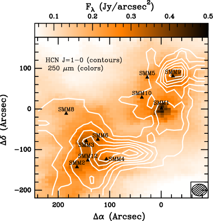
Figure 1: EMIR map of HCN 1-0 (contours) on top of the continuum emission at 250 $\mu$m from Herschel/SPIRE. The HCN contours start at 6 K km s^-1 (20 $\sigma$) and are drawn in steps of 3 K km s^-1 (10 $\sigma$). The protostellar properties are shown in Table 1.

The first detection of HCN toward a low-mass protostar NGC 1333 IRAS4B revealed a broad linewidth of 17.6 km s^-1 in HCN 4-3 similar to those of CO 2-1, and thus the HCN line was identified as a possible tracer of the outflows (Blake et al. 1995). Subsequent interferometric maps of Ser SMM1, SMM3, and SMM4 showed relatively compact emission on 30”$\times$30” scales (Hogerheijde et al. 1999). The line wings of HCN 4-3 were associated with the bipolar outflows and the line center with the cold envelope material. The HCN 1-0 emission was interpreted as a tracer of the outflow cavities (Hogerheijde et al. 1999). A recent survey of protostars in Perseus in HCN 4-3 shows its utility as a tracer of the most energetic outflows (Walker-Smith et al., 2014). Enhancement of HCN abundances in shocks where the gas temperatures above 200 K is suggested by both observations and models (Boonman et al. 2001, Lahuis et al. 2007, Pineau des Forets et al. 1990).

Mapping of CN emission toward the low-mass protostar, L483, shows an elongated structure in the outflow direction, which is narrower than that seen in the more quiescent gas and associated with the outflow cavity walls (Jørgensen 2004). Based on correlations between CN abundances and UV field in gaseous disks around more evolved sources, it was suggested that the enhancement of CN in L483 is related to the UV irradiation. Simultaneous mapping of HCN and CN on large scales indeed confirmed the offset of emission peaks between the two molecules in L1157 (Bachiller et al. 2001).

The presence of UV radiation around low-mass protostars was confirmed by the detection of warm gas traced by narrow ¹²CO 6-5 lines and spatially associated with outflow cavities in the low-mass protostar HH 46 (van Kempen et al., 2009b). Firm detection of [C i] 2-1 at the tip of the jet and the lack of CO was attributed to the dissociative bow shock, which itself is strong enough to produce UV photons that subsequently dissociate CO (Neufeld & Dalgarno, 1989; van Dishoeck et al., 2021). Their transport on $\sim$1000 AU scales is facilitated by the low densities and scattering in the outflow cavities (Spaans et al., 1995). Similar signatures of UV radiation were observed in a dedicated APEX-CHAMP⁺ survey of $\sim$20 protostars (Yıldız et al., 2012, 2015).

Far-infrared observations with Herschel provided access to highly-excited transitions of abundant molecules e.g., CO and H₂O, and detections of new species e.g., OH⁺ (Wyrowski et al., 2010) and H₂O⁺ (Ossenkopf et al., 2010). As part of the ‘Water in star-forming regions with Herschel’ (WISH, van Dishoeck et al., 2011, 2021) key program, a statistically significant sample of low-mass protostars was surveyed with the Heterodyne Instrument for the Far-Infrared (HIFI, de Graauw et al., 2010) and the Photodetector Array Camera and Spectrometer (PACS, Poglitsch et al., 2010). Among the key findings are: (i) ubiquitous gas at temperature of $\sim$300 K with molecular signatures resembling shocks (Herczeg et al., 2012; Goicoechea et al., 2012; Karska et al., 2013, 2018; Green et al., 2013; Manoj et al., 2013); (ii) a consistently low abundance of H₂O of $\sim 10^{-6}$ (Kristensen et al., 2017); (iii) high abundances of the H₂O photodissociation products and other hydrides, in particular OH (Wampfler et al., 2013; Benz et al., 2016); (iv) velocity-resolved components in H₂O profiles arising close to the protostar, at the positions of hydrides (Kristensen et al., 2013); (v) ratios of H₂O/OH and CO/OH consistent with UV-irradiated shock models (Karska et al., 2018). These results indicate that UV photons affect the physical and chemical structure in the immediate surroundings of low-mass protostars.

In this paper, we perform a ground-based follow-up study on large-scale maps of HCN and CN toward a low-mass star-forming region in the Serpens Main. The CN/HCN ratio is an independent tracer of UV photodissociation, which allows to benchmark the results from Herschel. We address the following questions: What is the morphology and spatial extent of the regions affected by UV radiation? Do chemical models validate the utility of this ratio as a tracer of UV-irradiated gas in low-mass star-forming regions? What is the UV field distribution in Serpens Main?

The paper is organized as follows: Section 2 describes the Serpens Main region and its protostars, the observations and data reduction. Section 3 shows the submillimeter maps and the line profiles at selected positions. Section 4 shows the determination of molecular column densities and their comparisons to the chemical model. Section 5 discusses the results in the context of complementary studies and Section 6 presents the summary and conclusions.

2 Source sample and observations

Table 1: Properties of targeted protostars in the Serpens Main region

Source	R.A.	Dec.	$T_{\mathrm{bol}}$	$L_{\mathrm{bol}}$	Class	Other names
	(J2000.0)	(J2000.0)	(K)	(L⊙)
SMM 1	18 29 50.0	+01 15 20.3	37	115.2	0	Ser-emb6, FIRS1, EC41, Bolo23
SMM 2	18 30 00.5	+01 12 57.8	34	7.2	0	Ser-emb4, Bolo28
SMM 3	18 29 59.6	+01 13 59.2	35	7.1	0	Ser-emb26, Bolo26
SMM 4	18 29 57.0	+01 13 11.3	68	5.1	I	Ser-emb22, Bolo25
SMM 5	18 29 51.4	+01 16 38.3	151	3.7	I	Ser-emb21, EC53, WMW24, Bolo22
SMM 6	18 29 57.8	+01 14 05.3	532	43.1	I	Ser-emb30, EC90, WMW35, SVS20S, Bolo 28
SMM 8	18 30 01.9	+01 15 09.2	15	0.2	0	Bolo30
SMM 9	18 29 48.3	+01 16 42.7	33	11.0	0	Ser-emb8, ISO241, WMW23, Bolo22
SMM 10	18 29 52.3	+01 15 48.8	79	7.1	I	Ser-emb12, WMW21, Bolo 23
SMM 12	18 29 59.1	+01 13 14.3	72	10.0	I	Ser-emb19, Bolo28

Table 2: Catalog of the observed molecular lines with IRAM and APEX

Mol.	Trans.	$E_{\mathrm{u}}/k_{\mathrm{B}}$	$n_{\mathrm{crit}}$	Freq.	Telescope	Beam size	Efficiency
		(K)	(cm-3)	(GHz)		($\arcsec$)	$\eta_{\mathrm{MB}}$
HCN	1-0	4.25	$1.7\times 10^{5}$	88.631847	IRAM-EMIR	28	0.81
H13CN	1-0	4.14	$1.3\times 10^{6}$	86.340184	IRAM-EMIR	29	0.81
	2-1	12.43	$1.2\times 10^{6}$	172.677881	IRAM-EMIR	14	0.68
CN	1-0	5.45	$1.1\times 10^{5}$	113.490985	IRAM-EMIR	22	0.78
C34S	3-2	13.9	$4.4\times 10^{5}$	144.617109	IRAM-EMIR	16	0.74
CS	3-2	14.1	$2.6\times 10^{5}$	146.969029	IRAM-EMIR	16	0.74
12CO	6-5	116.2	$1.0\times 10^{5}$	691.473076	APEX-CHAMP+	9	0.48
C18O	6-5	110.6	$2.6\times 10^{5}$	658.553278	APEX-CHAMP+	10	0.48

2.1 Serpens as a low-mass star-formation site

Serpens Main is a well-studied low-mass star-forming region located at a distance of 436$\pm$9 pc (Ortiz-León et al., 2017). The identification and classification of young stellar objects (YSOs) was done in the region as part of the Spitzer ‘From Molecular Cores to Planet-forming Disks’ (c2d) survey (Harvey et al., 2007; Enoch et al., 2009; Evans et al., 2009; Dunham et al., 2015). Submillimeter sources were studied using continuum observations at 12, 25, 60, 100 $\mu$m (Hurt & Barsony, 1996), 800, 1100, 1300, 2000 $\mu$m (Casali et al., 1993) and 3 mm (Testi & Sargent, 1998). The outflow activity in Serpens Main was characterized using CO 2-1 (Davis et al., 1999), and more recently with CO 3-2 and CO 6-5 for a subsample of sources (Graves et al. 2010, Dionatos et al. 2010, Yıldız et al. 2015). Ser SMM1, SMM3 and SMM4 were observed with Herschel as part of the WISH and ‘Dust, Ice, and Gas in Time’ (DIGIT, Green et al., 2013, 2016; Yang et al., 2018) programs.

Figure 1 shows the continuum map at 250 $\mu$m corresponding to the region we observed with the IRAM 30 m. The map was obtained with the Herschel Spectral and Photometric Imaging REceiver (SPIRE; Griffin et al. 2010) as part of the ‘Herschel Gould Belt Survey project’ (André et al. 2010).

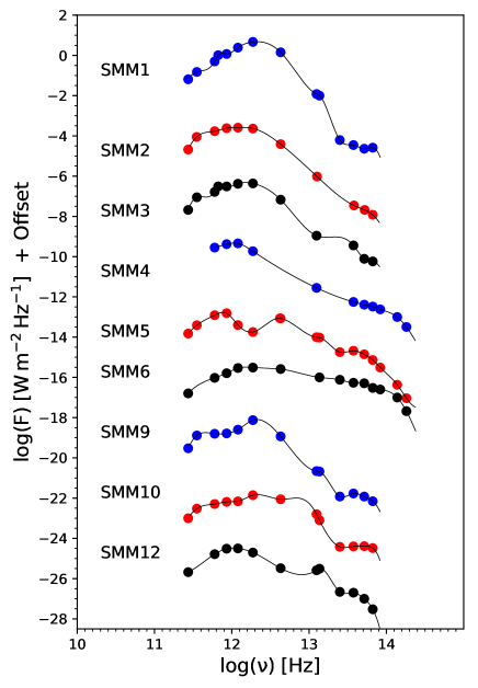
Figure 14: SED of protostars in the Serpens Main region. The offset between each plot is 3 orders of magnitude.

For the purpose of our analysis, we re-calculated the spectral energy distributions (SEDs) for all protostars in the region using the new continuum measurements at 70, 160, 250, 350 and 500 $\mu$m from PACS and SPIRE covering the peak of the SEDs and following the procedures outlined in André et al. (2010), Kirk et al. (2013), Könyves et al. (2015). Figure 14 and Table 6 show the SEDs of the protostars and provide the flux density at each wavelength. Table 1 shows the bolometric luminosities, temperatures and the classification of the sources based on Evans et al. (2009). We note that Ser SMM1 has a bolometric luminosity consistent with intermediate-mass protostars. However, it is known to consist of 5 protostars contributing to the total luminosity, and we regard it as a boarderline low-mass protostar (Hull et al. 2017).

2.2 Observations and data reduction

The observations at the IRAM 30 m telescope were performed between 14-Jul-2009 and 17-Jul-2009 as part of the project ‘HCN/CN as UV-tracers in YSO envelope-outflow interfaces’ (PI: L. Kristensen). The Eight MIxer Receiver (EMIR) bands E090 and E150 were used to observe HCN 1-0, CN 1-0 and CS 3-2, and provided also additional detections of C³⁴S 3-2, H¹³CN 1-0 and H¹³CN 2-1. The frequency range covers $\pm$ 53.59 MHz from the central line. The backend was the Versatile SPectrometer Array (VESPA) autocorrelator and the 1 MHz filterbank reaching a spectral resolution of 39 kHz (E150 band) and 78 kHz (E090 band). Table 2 shows the full list of molecular transitions observed with EMIR with the respective frequency-dependent beam sizes and main beam efficiencies, $\eta_{\mathrm{MB}}$ from 0.68 to 0.81, used to convert antenna temperatures to main beam temperatures ($T_{\mathrm{MB}}$).

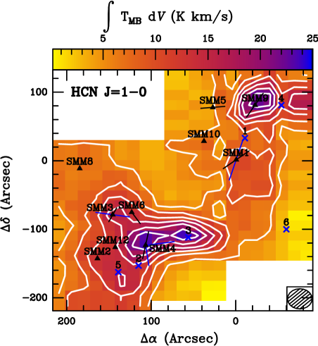
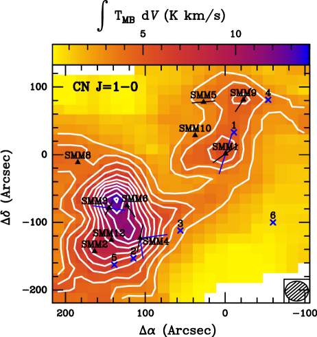
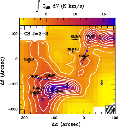
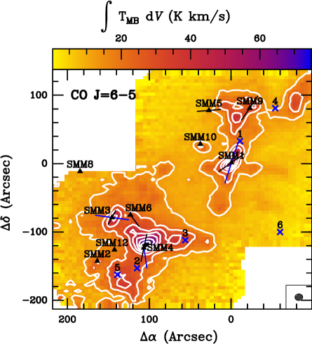
Figure 2: Integrated intensity maps of HCN 1-0 (upper left panel), CS 3-2 (upper right panel), CN 1-0 (bottom left panel) and CO 6-5 (bottom right panel) toward the Serpens Main star-forming region shown in contours and colors. Black triangles show the positions of protostars (see Table 1) and blue crosses show the outflow positions selected for analysis (see Table 3). Solid lines show outflow directions from CO 6-5 (black; Yıldız et al. 2015) and CO 3-2 (blue; Dionatos et al. 2010). The center of the maps (0,0) corresponds to ($\alpha$, $\delta$) = 18^h29^m49$\aas@@fstack{s}$6, +01$\degr$15$\arcmin$20$\aas@@fstack{\prime\prime}$5. Contour levels start at 20 $\sigma$ (6 K km s^-1), 10 $\sigma$ (3 K km s^-1), 7 $\sigma$ (3.5 K km s^-1) and 70 $\sigma$ (14 K km s^-1) with steps of 10 $\sigma$, 3 $\sigma$, 3.5 $\sigma$ and 50 $\sigma$, for HCN, CN, CS and CO respectively.

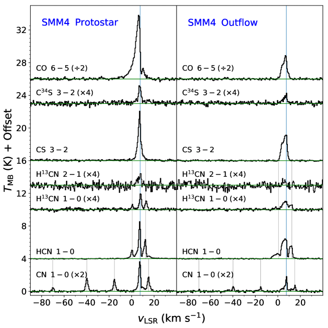
Figure 3: Line profiles of CO 6-5, C³⁴S 3-2, CS 3-2, H¹³CN 2-1, H¹³CN 1-0, HCN 1-0 and CN 1-0 lines at the protostellar position Ser SMM4 (left) and the associated outflow position no. 3 (right). Blue vertical lines show the main line component, and grey lines show the hyperfine splitting components. The maps in Figure 2 show the sum of all hyperfine components detected in the spectra of HCN and CN.

The on-the-fly (OTF) mapping mode was used in cross-directions to obtain two 340${}^{\prime\prime}\times 340^{\prime\prime}$ maps centered at ($\alpha_{\mathrm{J2000}}$,$\delta_{\mathrm{J2000}}$)=18^h29^m49$\aas@@fstack{s}$6, +01$\degr$15$\arcmin$20$\aas@@fstack{\prime\prime}$5, and 18^h29^m56$\aas@@fstack{s}$6, +01$\degr$14$\arcmin$00$\aas@@fstack{\prime\prime}$3. The merging and data reduction were carried out with the CLASS package within GILDAS. For the sake of analysis, the EMIR spectra were baseline-corrected and resampled to a resolution of 0.5 km s^-1, which is optimal for the observed linewidths in the range from $\sim$2 km s^-1 to $\sim$21 km s^-1 (Section 3.2). We fit a zeroth order baseline to all of the spectra in order to remove the continuum. The rms of extracted spectra varies from 0.024 K to 0.125 K in 0.5 km s^-1 bins (see Table 8). Figure 2 shows the size and extent of the maps after the merging of two datasets and beam convolution. The CN map was convoluted to a the beam size of HCN.

The CHAMP+ dual-beam heterodyne receiver on the Atacama Pathfinder Experiment (APEX) telescope used for CO 6-5 observations at 691.5 GHz was originally presented in Yıldız et al. (2015). The observations were performed on June 16th 2009 using position-switching in the OTF mode resulting in maps covering 340${}^{\prime\prime}\times 340^{\prime\prime}$. The Fast Fourier Transform Spectrometer (FFTS) was used as the backend with a resolution of 0.079 km s^-1 (Klein et al., 2006). The rms varies from 0.12 to 0.23 K in 0.5 km s^-1 bins (Table  8). Similarly, observations of the Ser SMM1 protostar in C¹⁸O 6-5 were obtained with the APEX/CHAMP+ on October 23th 2009. The data reduction and analysis were performed in a similar way to the IRAM observations using the CLASS software.

3 Results

In the following sections, we present IRAM 30 m maps and line profiles providing complementary information about the emission from protostars and their outflows, and large-scale cloud emission. Differences in spatial extent reflect the range of gas and dust distributions, and associated physical conditions and processes. We calculate ratios of various transitions to indicate species tracing similar physical components, the gas temperature, and line opacities.

3.1 Spatial extent of line emission

Figure 2 shows the line emission associated with protostars and their outflows in HCN, CN and CS lines obtained with IRAM 30 m and CO with APEX. The integrated line intensities in HCN and CN are the sum of all hyperfine components detected in the spectra (see Figure 3). Maps in H¹³CN 1-0 and C³⁴S 3-2 are presented in Appendix B.

HCN 1-0 emission is associated with clusters of protostars in the south-east and north-west parts of the map where dust emission at 250 $\mu$m is also detected (Figure 1). The emission peaks are the strongest at the positions of Ser SMM4 and SMM9 protostars and their outflows, and significantly weaker at Ser SMM1 and SMM3 - in part due to self-absorption in their line profiles (Figure A.3). Qualitatively, the pattern of emission in HCN is similar to the CO 6-5 - a well-established outflow tracer (Figure 2; bottom right panel). The enhancement of HCN emission along the outflow is in agreement with previous surveys of low-mass protostars (Bachiller et al., 2001; Walker-Smith et al., 2014). Any differences between HCN and CO likely stem from the higher critical density of the HCN 1-0, its lower upper energy level (see Table 2), and its significantly easier photodissociation due to UV photons than CO (see Section 5).

CS 3-2 emission shows a very similar spatial distribution compared to HCN 1-0 and CO 6-5, with most prominent structures associated with Ser SMM4. Some differences are seen, mostly in the surroundings of Ser SMM9, where CS emission is substantially weaker, in contrast to HCN which shows similar line strengths towards both protostars. Additionally, CS shows a relatively strong emission to the west of Ser SMM9, which coincides with the outflow from that protostar. The differences may result from CS 3-2 tracing higher-density gas than HCN 1-0 (Shirley, 2015).

In contrast to HCN and CS, CN 1-0 emission is more closely associated with the positions of protostars and the continuum peaks at 250 $\mu$m, but not with the outflows (Figures 1 and 2). The emission is the strongest towards Ser SMM4, SMM3, and SMM6, and the region in between these three protostars. The differences in spatial extent between CN and the outflow tracers suggest a different physical origin (see Section 5.1).

3.2 Detection rates and line profiles

To explore the gas properties in the Serpens Main, we select 10 protostellar positions, 5 outflow positions, and 1 position not associated with any known protostar. The selection benefits from previous observations of this star-forming region in other tracers and detections of line emission with IRAM (Figure 2). Figure 3 shows the line profiles of targeted species and transitions toward Ser SMM4 and one of its outflow positions. Appendix C shows the line profiles in the remaining positions.

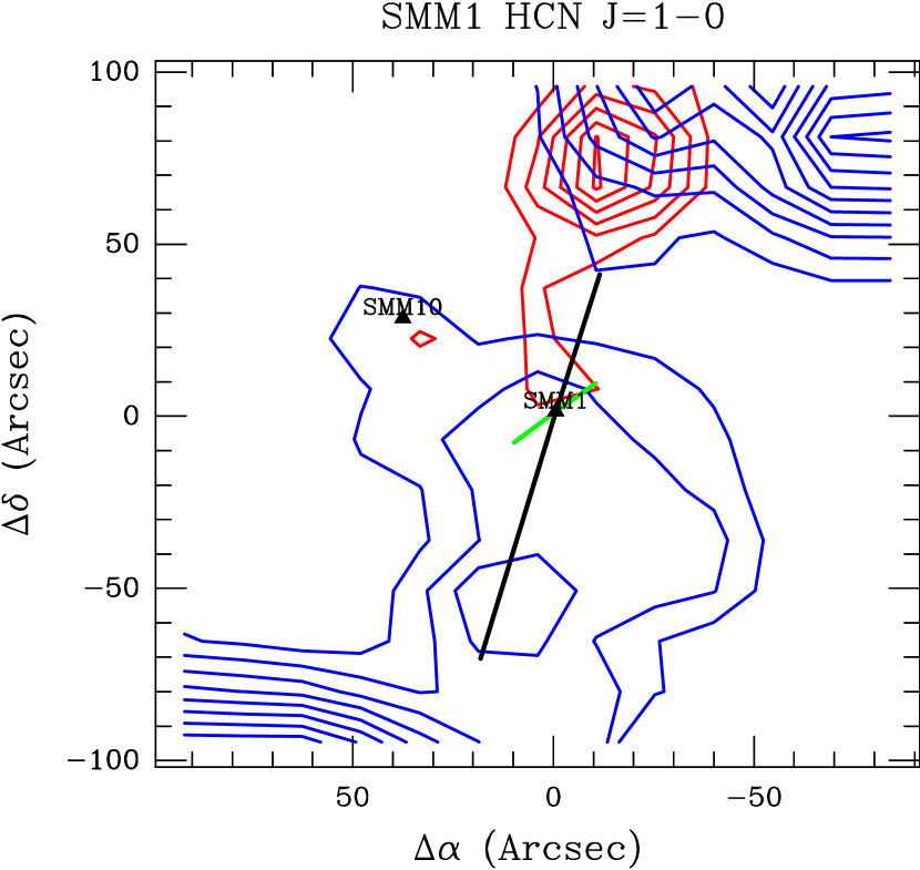
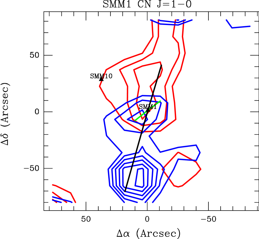
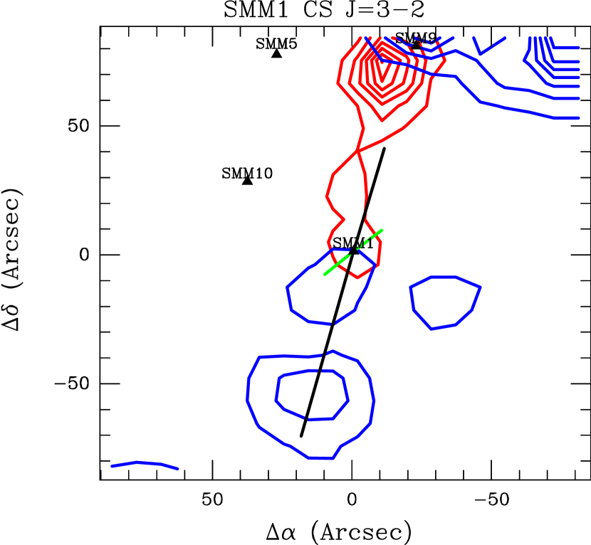
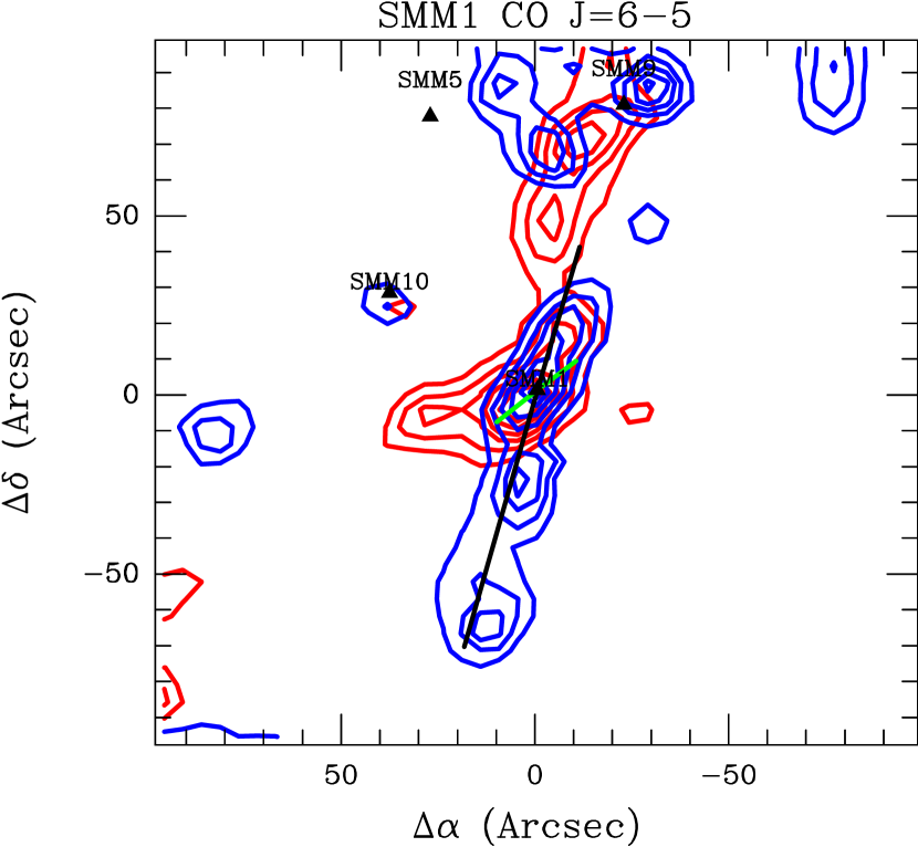
Figure 4: Emission in the line wings of HCN 1-0, CN 1-0, CS 3-2 and CO 6-5 toward Ser SMM1 (blue and red contours). The velocity ranges used to calculate the integrated intensities are provided in Appendix D. Black and green lines correspond to outflow directions in CO 3-2 and CO 6-5 (the same as in Figure 2).

All targeted species and their isotopologues are detected at the selected protostar positions in the Serpens Main region, except for H¹³CN 2-1 which is detected only towards Ser SMM4 and Ser SMM9. Similarly, emission in the outflow positions is always detected in HCN, CS, CN and CO. Considering the targeted rare isotopologue lines, detections are seen in C³⁴S 3-2 , H¹³CN 1-0, but not in H¹³CN 2-1. In the case of HCN and CN, up to 3 and 5 components are detected as the result of the hyperfine splitting, respectively.

The line shapes at both the protostar and outflow positions show relatively broad profiles, with outflow wings in CS extending to 13.6 km s^-1 and 9.8 km s^-1 at the protostellar and outflow positions, respectively (Figure 3). Clearly, the beam sizes of IRAM encompass a substantial amount of outflow emission even at the protostellar position.

In order to quantify the emission in the line wings, we use the line profile of C¹⁸O 6-5 towards Ser SMM1, which is a well-established envelope tracer based on high S/N observations and modeling (Kristensen et al. 2010, Yıldız et al. 2013). The velocity range for the C¹⁸O line sets the limits for the inner velocity ranges for the line wings in the observed transitions (Figure 19 in Appendix  D). The outer velocity ranges are calculated separately for each line based on the signal detected above 2$\sigma$, selected by the visual inspection of the line profiles.

Figure 4 shows the subset of the IRAM 30m large-scale maps toward Ser SMM1 where emission is integrated solely in the line wings velocity range. Emission in HCN, CN, and CS resembles that of warm gas in the outflows traced by CO 6-5, but some differences in morphology are clearly present. For example, HCN emission in line wings in the close vicinity of Ser SMM1 is much weaker than that of CN, which cannot be assigned to the self-absorption of material in the envelope. Low HCN emission might be rather related to the presence of large cavities around Ser SMM1, where ionizing radiation is capable of photodissociating HCN (Hull et al. 2016, Hull et al. 2017). A full analysis of the outflow properties will be presented in a forthcoming paper (Karska et al., in preparation).

In the case of Ser SMM4 (Figure 3), the emission in the line wings of CS 3-2 is 61% of the total profile at the protostellar position and 72% at the outflow position. Similar characteristics is seen in HCN line wings (48% and 68%, respectively). In contrast, CN 1-0 is detected mostly at source velocity, with 40% of emission in the line wings. Among all 15 positions, exceptionally broad line wings in HCN and CS are detected at the Ser SMM1, Ser SMM9 and Ser SMM10 protostellar positions and outflow positions nr 1, 4, and 5, exceeding 70% of the total profile in HCN and 58% in CS. In fact, these high fractions of line emission in the wings are upper limits, because the opacity effects decrease the emission primarily in the source positions. In case of the weaker lines like CN, the fraction of wing versus on-source emission might be slightly lowered due to a limited signal-to-noise ratio of the spectra, which might not recover the wings at full. Higher signal-to-noise observations of rare isotopologue lines as well as CN would be needed to fully recover the on-source and wing emission.

The shapes of line profiles clearly indicate that the emission in various species is detected in different physical components of the protostellar systems. For the forthcoming analysis, we will consider the emission in the line wings alone and in the fully integrated profiles separately.

3.3 Line ratios

In this section, we calculate molecular line ratios at protostar and selected positions in the Serpens Main region separately for the fully integrated profiles and for the line wings. We discuss (i) the ratios of different isotopologues, constraining the line opacities, and (ii) the ratios of different species, reflecting their differences in spatial extent and relative abundances.

3.3.1 Ratios of different isotopologues

The line ratio of the same transition of two isotopologues is a tracer of line opacity of the more abundant species, assuming that the emission in the other isotopologue is optically thin. We calculate line opacities of HCN 1-0 and CS 3-2 lines both at the protostellar and outflow positions using (Goldsmith et al., 1984; Mangum & Shirley, 2015):

$$\frac{T_{\mathrm{HCN}}}{T_{\mathrm{H^{13}CN}}}=\left(\frac{\nu_{\mathrm{HCN}}}{\nu_{\mathrm{H^{13}CN}}}\right)^{2}\frac{X[\mathrm{HCN}]}{X[\mathrm{H^{13}CN}]}\frac{1-\exp(-\tau_{\mathrm{HCN}})}{\tau_{\mathrm{HCN}}},$$ (1)

where $X_{\mathrm{i}}$ and $T_{\mathrm{i}}$ refer to the abundance and antenna temperature of the isotopologue, and the same excitation for both isotopologues is assumed. We adopt an abundance ratio of HCN and H¹³CN following the standard interstellar ratio of ¹²C/¹³C of 68 (Milam et al., 2005), and 20 for the CS and C³⁴S abundance ratio (Tercero et al., 2010), and assume that both isotopologues arise from the same physical region, described by the excitation temperature, $T_{\mathrm{exc}}$, and in local thermodynamic equilibrium (LTE).

Optical depths at the protostellar positions range from $\sim$2.3 to 12.8 for HCN and from $\sim$0.3 to 4.4 for CS when the emission from the entire profile is considered (see Table 13). At the outflow positions, the optical depths are $\sim$4.9-8.0 for HCN and $\sim$0.6-4.9 for CS. These values are in fact lower limits, because line profiles of HCN and CN show self-absorption toward many positions (see Figures 17 and 18). To avoid this effect, we calculate optical depths in the line wings alone.

HCN emission is optically thin ($\tau<1$) in the line wings towards the Ser SMM3, SMM5, and SMM10 protostellar positions (which also include emission from the outflows) and pure outflow positions 1 and 2. CS emission is optically thin in Ser SMM3, SMM6, and SMM10, and outflow position 3. In the remaining positions, $\tau$ ranges from 1.3 to 2.7 (HCN) and from 1.2 to 5.6 (CS), indicating optically thick emission.

The optical depth of the CN emission is calculated using the ratios of its hyperfine-splitted components using entire line profiles. The ratio of the F=3/2$\rightarrow$1/2, F=5/2$\rightarrow$3/2, and F=1/2$\rightarrow$1/2 components is 0.1235:0.3333:0.0988 in the optically thin limit (Skatrud et al., 1983; Endres et al., 2016). We find that CN lines are generally optically thin toward the selected positions, with the exception of Ser SMM1, SMM5, and SMM10 where $\tau$ is $\sim 1.1-2.1$ for the two strongest components (see Table 13).

Similar method is used to verify the assumption that the H¹³CN emission is optically thin. We use the ratios of the HCN hyperfine-splitted components as a proxy for H¹³CN following Loughnane et al. (2012). The ratio of the F=2$\rightarrow$1 to F=1$\rightarrow$1 lines, which is a recommended tracer by Mullins et al. (2016), indicates optical depths in the range from 0.77 to 2.76, and a median of 1.29 (see Table E.4). Thus, the line is optically thick toward some positions, and may not provide a reliable benchmark for HCN. The optical depths of HCN determined using hyperfine-splitted components show $\tau_{\mathrm{HCN}}$ in the range from 1.48 to 4.12, with a median of 2.74. These values are generally lower than those determined using H¹³CN, but do not change the conclusion that HCN is optically thick.

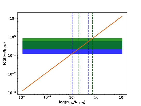
Figure 5: The ratio of CN to HCN column densities obtained with RADEX for $n_{\mathrm{H}}=10^{5}$ cm^-3 and $T_{\mathrm{kin}}=50$ K for a range of line intensity ratios (orange line). The observed line intensity ratio is shown as a rectangle: light green color corresponding to the values observed at the protostar position, blue color for the outflow positions and dark green color for both regions. Column density ranges are marked with black and navy emdashed lines for protostars and outflow positions, respectively.

Table 3: Model-dependent column density ratios of CN to HCN at protostar and off-source positions

$n_{\mathrm{H_{2}}}$	$T_{\mathrm{kin}}$	$N_{\mathrm{CN}}$/$N_{\mathrm{HCN}}$	$N_{\mathrm{CN}}$/$N_{\mathrm{HCN}}$
$($cm${}^{-3})$	(K)	Protostars	Off-source
104	50	1.57-5.55	0.85-3.79
104	100	1.40-4.98	0.76-3.40
104	200	1.33-4.70	0.72-3.21
104	300	1.32-4.66	0.71-3.18
104	400	1.45-5.13	0.78-3.50
104	500	1.56-5.53	0.85-3.77
105	50	1.85-6.55	1.00-4.67
105	100	1.87-6.23	1.01-4.52
105	200	2.01-7.12	1.09-4.86
105	300	2.14-7.60	1.16-5.18
105	400	2.22-7.87	1.20-5.37
105	500	2.27-8.02	1.23-5.47
106	50	2.52-8.93	1.37-6.10
106	100	2.84-10.04	1.54-6.85
106	200	3.17-11.22	1.72-7.65
106	300	3.33-11.80	1.80-8.05
106	400	3.01-10.67	1.63-7.28
106	500	2.75-9.73	1.49-6.64

Qualitatively, the optical depths determined for HCN, CS, and CN are in agreement with simple calculations for total line profiles using the 1D non-LTE radiative-transfer code RADEX (van der Tak et al., 2007). Adopting a hydrogen density of $10^{5}$ cm^-3 and a gas kinetic temperature of 50 K typical for low-mass protostars (Mottram et al., 2014), we find optical depth of CS 3-2 line as 2.1, assuming column densities of $5\times 10^{13}$ cm^-2. Using a revised collisional rates for HCN adopted from Mullins et al. 2016, the optical depth calculated for HCN 1-0 is 2.9, assuming column densities of $3\times 10^{14}$ cm^-2. This value is in agreement with the optical depth calculated from F=2$\rightarrow$1 to F=1$\rightarrow$1 ratio. Similar optical depths (within a factor of 2) are found for gas temperatures of 300 K and number densities of $10^{4}$ cm^-3.

In summary, HCN 1-0 and H¹³CN 1-0 are optically thick, and CN 1-0 is typically optically thin. Thus, the opacity effects influence the relative spatial distribution of CN and HCN, and their ratio.

3.3.2 Ratios of different species

Line ratios of various species show differences related to their local abundances and excitation conditions. The CN/HCN intensity ratio is expected to trace regions affected by UV radiation.

Protostars with the highest CN/HCN intensity ratio, where the impact of UV might be the strongest, are located in the south-east subcluster. Here, the peak of CN 1-0 emission is detected close to Ser SMM3 and SMM6 (Figure 2). Both protostars drive outflows detected in CO 6-5, and less clearly in HCN (see also Figure C.1). In fact, the HCN/CO ratio at Ser SMM3 and SMM6 is on the low side (0.27 and 0.44 respectively) compared to the average of 0.41$\pm$0.22 for protostar positions and 0.59$\pm$0.23 for off-sources positions (Table 3).

The lowest CN/HCN intensity ratio is seen toward Ser SMM9, and to a lesser extent toward Ser SMM8 and SMM10. The former source drives a large outflow, where bright emission in HCN likely results from its high abundance in the warm gas (similarly to off-source position 3). The latter sources are characterized by a very weak molecular emission in general (Figure 2). Ser SMM8 is a low luminosity sources ($L_{\mathrm{bol}}$ of 0.2 $L_{\odot}$, see Table 1), which is located on the map edge in CO 6-5. Ser SMM10 is associated with CO 6-5 peak, but is clearly very weak in both CN and HCN.

The median value of the CN to HCN intensity ratio at the protostellar positions is $0.63\pm 0.19$. Taking into account the emission in the line wings, the ratio is slightly lower and equals $0.40\pm 0.18$. It is generally consistent with the ratios measured for each source using the full profile. The ratio calculated for the selected off-source positions equals $0.43\pm 0.18$ and $0.20\pm 0.18$, for the full profile and wings, respectively.

The CN/HCN intensity ratio for the Class 0 protostars is $0.61\pm 0.23$ and for the Class I protostars is $0.67\pm 0.17$, indicating that the evolutionary stage does not strongly affect the measured ratios. A slightly higher CN/HCN ratio for Class I protostars is consistent with increasing opening angles of the outflows for more evolved sources and larger areas affected by UV radiation (see Discussion). The opacity effects overestimate the ratio of CN and HCN, and could have a slightly stronger impact on the more massive envelopes of Class 0 sources (Section 3.3.1).

4 Analysis

In this section, we calculate column densities of the molecules with the radiative-code RADEX (van der Tak et al., 2007) and compare them to the results from the chemical-code Nahoon, run for a set of gas temperatures, densities and UV radiation fields.

4.1 Column densities of molecules from observations

In case of optically thin lines and LTE conditions, the column density of the upper level of a given molecule, $N_{\mathrm{u}}$, can be calculated using Equation 2, where $\beta=8\pi k/hc^{3}$ is a constant equal to 1937 cm^-2, $W$ is the integrated intensity of the emission line ($\int{T_{mb}\,dV}$), $A$ is the Einstein coefficient and $\nu$ is the transition frequency between the upper and lower level expressed in GHz (e.g., Yıldız et al., 2015).

$$N_{\mathrm{u}}=\beta\,\frac{\nu\,W}{A}$$ (2)

In order to calculate the total column density of a given molecule, we use the following expression and adopt a gas temperature of 50 K (Yıldız et al., 2012).

$$N_{\mathrm{tot}}=Q(T_{\mathrm{exc}})\,\exp(\frac{E_{\mathrm{u}}}{k_{\mathrm{B}}\,T_{\mathrm{exc}}})\frac{N_{\mathrm{u}}}{g_{\mathrm{u}}},$$ (3)

where $Q$($T$) refers to the temperature-dependent partition function for the given molecule, $E_{\mathrm{u}}$ is the upper energy level, $g_{\mathrm{u}}$ is level degeneracy, and $k_{\mathrm{B}}$ is the Boltzmann constant. Appendix D shows the column densities obtained for all molecules, both at the protostellar and the outflow positions.

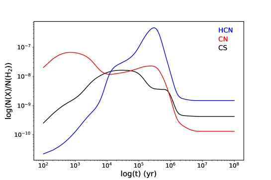
Figure 6: Time evolution of CN (red line), HCN (blue line) and CS (black line) abundances obtained with Nahoon astrochemical code with initial parameters of $n_{\mathrm{H}}=10^{4}$ cm^-3, $T=10$ K, $A_{\mathrm{V}}$ = 5 mag. The initial abundances of CN, HCN and CS equal zero at $t=0$. The assumed cosmic-ray ionization rate is $1.3\times 10^{17}$ s^-1, dust to gas mass ratio is 0.01, dust grain radius is $10^{-5}$ cm and grain density is 3 g cm^-3.

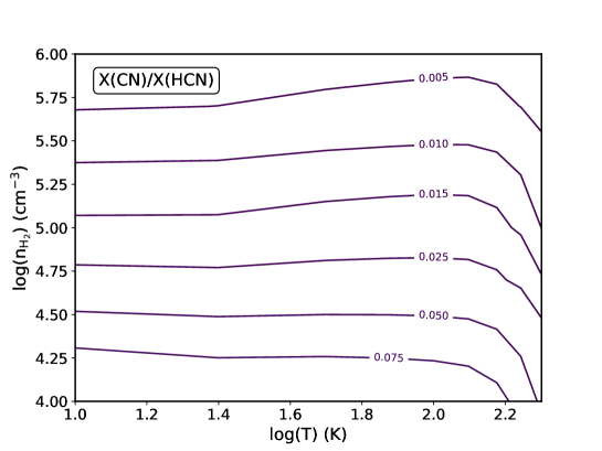
Figure 7: Contour plot of Nahoon sets of models of CN/HCN abundances ratio with fixed visual extinction $A_{\mathrm{V}}$ = 5 mag and 10⁷ yr after star formation began in the cloud.

Because of the optical thickness of HCN (Section 3.3.1), we also employ the non-LTE radiative transfer code RADEX to obtain independent determinations of the column densities. In order to mimic the optically thin case, for the calculations we adopt a HCN column density of 10⁸ cm^-2. We vary the column density of CN from 10⁶ to 10¹⁰ cm^-2. The calculations are computed assuming a linewidth of 1.0 km s^-1 for typical physical conditions of the gas in low-mass star forming regions - the number densities, $n_{\mathrm{H}}$ of the order of $10^{4}$-$10^{6}$ cm^-3 and the kinetic temperatures, $T_{\mathrm{kin}}$, of 50-300 K (Yıldız et al., 2013; Mottram et al., 2014). The models include hyperfine splitting, but no internal radiation field.

Figure 5 shows an example model calculated for a density of $10^{5}$ cm^-3 and kinetic temperature of 50 K, and its comparison to observations. The preimage of the observed line intensity ratios is equal to the ratios of column densities. Table 3 shows calculations for various sets of $n_{\mathrm{H}}$ and $T_{\mathrm{kin}}$. The column densities ratios of CN to HCN increase both as a function of density and temperature, but their resulting range is relatively narrow. For the protostellar positions, the CN/HCN column density ratios are in the range from 1.3 to 11.8 ($1\sigma=3.2$). In case of off-source positions, which likely represent a larger variety of environments, the CN/HCN column densities range from 0.7 to 8.1 ($1\sigma=2.3$). Thus, the observed line ratios correspond to column densities ratios of the order of $\sim$1-12 irrespective of the gas parameters.

4.2 Chemical model

Table 4: Dominant processes in CN and HCN chemistry at 50 K

Molecule	Weak UV fields	Medium UV fields	Strong UV fields
	(G0 = $10^{-3}-10^{-1})$	(G0 = $10^{-1}-10^{1})$	(G0 = $10^{1}-10^{6})$
CN	Destruction
	O + CN $\rightarrow$ N + CO	CN + h$\nu$ $\rightarrow$ C + N	CN + h$\nu$ $\rightarrow$ C + N
	CN + N $\rightarrow$ C + N2	O + CN $\rightarrow$ N + CO
	Production
	N + CH $\rightarrow$ H + CN	N + C2 $\rightarrow$ C + CN	HCN+ + e- $\rightarrow$ H + CN
	CNC+ + e- $\rightarrow$ C + CN	H + CN+ $\rightarrow$ CN + H+	N + CH $\rightarrow$ H + CN
	N + C2 $\rightarrow$ C + CN		H + CN+ $\rightarrow$ CN + H+
			N + C2 $\rightarrow$ C + CN
HCN	Destruction
	HCN + C+ $\rightarrow$ H + CNC+	HCN + C+ $\rightarrow$ H + CNC+	HCN + h$\nu$ $\rightarrow$ H + CN
	HCN + H+ $\rightarrow$ H + HNC+
	HCN + h$\nu$ $\rightarrow$ H + CN
	Production
	N + CH2 $\rightarrow$ H + HCN	H + CCN $\rightarrow$ C + HCN	HCNH+ + e- $\rightarrow$ H + HCN
	H + CCN $\rightarrow$ C + HCN	HCNH+ + e- $\rightarrow$ H + HCN	H + CCN $\rightarrow$ C + HCN
	HCNH+ + e- $\rightarrow$ H + HCN

The Nahoon chemical code is used to calculate theoretical abundances of molecules for a set of physical conditions and UV field strengths. It is a well-known almost purely gas-phase chemical code for astronomical applications (Wakelam et al. 2015). The Nahoon solver computes the chemical evolution in time including 489 species and 7509 gas-phase and selected gas-grain reactions based on rate coefficients from the Kinetic Database for Astrochemistry (KIDA) database.

The UV radiation in Nahoon is described through the relation between the visual extinction $A_{\mathrm{V}}$ and the photodissociation rate coefficient $k$ as follows:

$$k=\alpha e^{-\gamma A_{\mathrm{V}}},$$ (4)

where, $\mathrm{\alpha}$ and $\mathrm{\gamma}$ are the coefficients of photodissociation for HCN, equal to $1.64\times 10^{-9}$ s^-1 and $3.12$ s^-1, respectively (Heays et al., 2017).

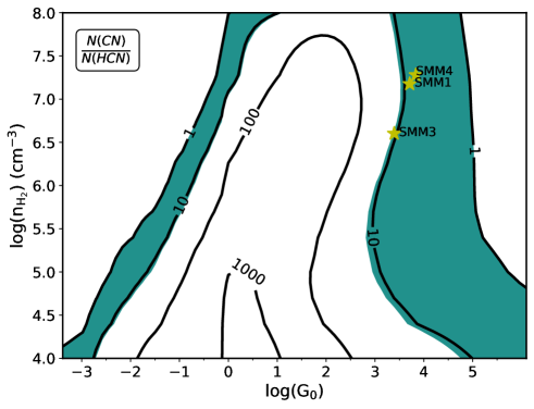
Figure 8: The column density ratio of CN to HCN from Nahoon for a range of hydrogen densities and UV field strengths assuming $T=50$ K. The corresponding range of ratios from observations and radiative transfer models are shown in green (see Table 4). Yellow stars show the positions of Ser SMM1, SMM3, and SMM4 assuming their gas number densities at 1000 AU from Kristensen et al. (2012).

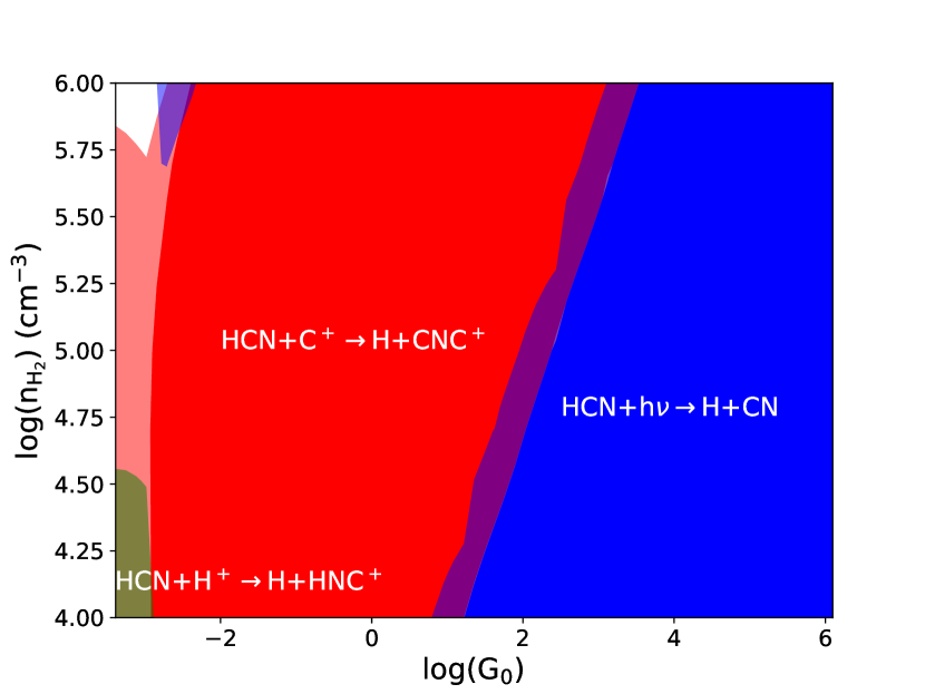
(a)

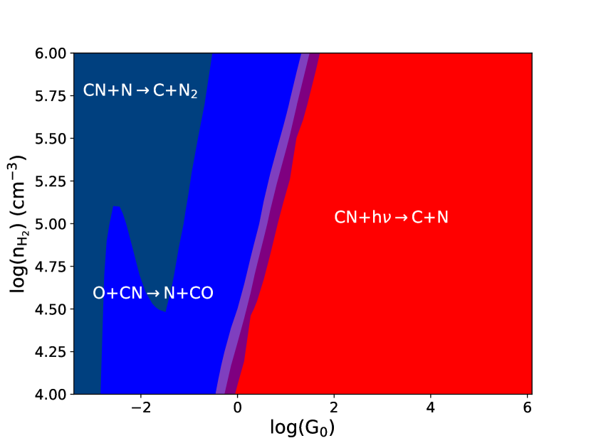
(b)

Figure 9: Dominant reactions of HCN destruction (left) and CN destruction (right) assuming $T\leavevmode\nobreak\ =\leavevmode\nobreak\ 50$ K. Reactions contributing at least to 50$\%$ of the total flux are marked with full colors. Transparent colors at the borders of different regimes correspond to 30$\%$-50$\%$ contribution.

The evolution of the chemical network starts at the time of dense cloud formation. Figure 6 shows a model corresponding to a typical dense cloud with a temperature of 10 K and hydrogen total density of $n_{\mathrm{H}}=10^{4}$ cm^-3. The chemical composition of the CN, HCN and CS molecules becomes stable after $10^{7}$ yr; the HCN abundance is higher than that of CN. Assuming that star-formation begins at $t=10^{6}$ yr in a dense cloud, we use model abundances for all 489 species at this time as an input data for the forthcoming set of models.

The closest neighborhood of low-mass protostars is simulated based on the initial abundances of all species from the modeling of pre-stellar cores. We adopt a cosmic-ray ionization rate of $1.3\times 10^{17}$ s^-1 (Cravens & Dalgarno, 1978). The sets of models are run for a temperature range between 10 and 200 K and a total hydrogen densities from $10^{4}$ cm^-3 to $10^{6}$ cm^-3.

Figure 7 shows the model results assuming a visual extinction of 5 mag which corresponds to a lack of UV radiation. In that case, HCN is more abundant than CN by about 2-3 orders of magnitude. The column density ratio of CN to HCN weakly depends on the gas temperature until $\gtrsim 100$ K, so we fix the gas temperature at 50 K.

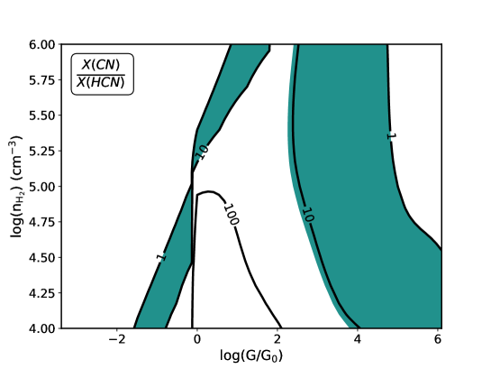
Figure 21: The column density ratio of CN to HCN from Nahoon for a range of hydrogen densities and UV field strengths assuming $T=300$ K. The corresponding ratios from observations and radiative transfer models are shown in green.

Figure 8 shows the abundance ratio of CN to HCN as a function of $n_{\mathrm{H}}$ and G₀ (at $T=50$ K), where G₀ is the far-ultraviolet radiation field (6 eV$<h\nu<13.6$ eV) in the units of the Habing Field, $1.6\times 10^{-3}$ ergs cm^-2 s^-1 (Habing, 1968; Kaufman et al., 1999). The models show a weak impact of hydrogen number densities on the $N_{\mathrm{CN}}$/$N_{\mathrm{HCN}}$ ratio, which mostly depends on the value of G₀. The ratio increases with G₀ until it equals $\sim 1$. Subsequently, the $N_{\mathrm{CN}}$/$N_{\mathrm{HCN}}$ decreases for higher G₀. Similar calculations performed at 300 K show a very similar pattern (See Fig. 21).

The $N_{\mathrm{CN}}$/$N_{\mathrm{HCN}}$ ratios obtained from observations and radiative transfer models are $\sim 1-12$ (see Section 4.1). Chemical models are consistent with the observed column density ratio of CN to HCN for UV fields that are 10³ larger than the average interstellar value (Figure 8). The observations are also consistent with models with significantly lower UV fields, of 10^-3-10^-2 times the average interstellar UV field. For three sources observed with Herschel, gas densities at 1000 AU and independent signatures of UV fields were found (Kristensen et al., 2012, 2017; Karska et al., 2018). Using Figure 8, we estimate $G_{\mathrm{0}}$ toward Ser SMM1, SMM3 and SMM4 of $10^{3}-10^{4}$ the interstellar value. We discuss these values and compare them to other measurements in Section 5.3.

In order to understand the chemistry leading to the CN/HCN$>1$ in the presence of UV fields, both production and destruction of each molecule need to be investigated. Table 4 shows the dominant reactions at 50 K for three UV field regimes - weak (G₀ = $10^{-3}-10^{-1}$), medium (G₀ = $10^{-1}-10^{1})$, and strong (G₀ = $10^{1}-10^{6})$. These reactions account for more than 80$\%$ of accumulated total flux of all reactions, where the reaction flux is defined as reactants’ abundances multiplied by the reaction rate coefficient. Additional reactions, where CN or HCN production or destruction is greater than 30$\%$, are listed in Appendix F.

In the regime of strong UV fields (G${}_{0}>10^{1}$), the dominant destruction route of both HCN and CN is photodissociation by UV photons. Similarly, in medium UV fields CN is also directly destroyed by UV photons, and HCN is removed by the reaction with C⁺, which production also requires UV radiation. At a gas temperature of 300 K, corresponding to the bulk of gas in the outflows from low-mass protostars (Karska et al., 2018), the impact of photodissociation of HCN becomes dominant already in the medium UV fields (see Appendix F). For low UV fields, the main destruction route of CN by collisions with H₂ leads to the production of HCN, and subsequent decrease in the CN/HCN ratio.

Figure 9 shows which reactions dominate the molecular destruction for a range of UV fields and also gas densities. HCN and CN photodissociation is more efficient at lower densities, and stronger UV fields are required to maintain photodissociation in denser regions. Clearly, outflow cavities carved by jets and winds in the envelopes of protostars facilitate the irradiation of the bulk of gas (see also Spaans et al., 1995; van Kempen et al., 2009a).

To summarize, the astrochemical models calculated using the Nahoon code reproduce the observed CN/HCN ratios in the Serpens Main for UV fields in the range from $10^{3}$ to $10^{5.5}$ times the interstellar radiation field, assuming gas densities of 10⁵ cm^-3. Independent measurements of gas densities in individual protostars are needed to narrow down the determination of G₀ for specific objects. Clearly, the strength of the UV field has an important effect on the chemical reactions at play and the resulting abundance ratios of molecules.

5 Discussion

5.1 Spatial extent of HCN and CN in low-mass protostars

The immediate environment of protostars is subject to multiple physical and chemical processes which can be traced using a broad range of molecules and their transitions. Here, we propose to use the CN to HCN ratio as a tracer of UV irradiation associated with low-mass star formation on cluster scales ($\sim$1 pc).

Large-scale emission from both CN and HCN is clearly detected in the Serpens Main (Figure 10, see also Section 3.1). The HCN emission shows a more extended pattern, but overall the emission peaks of both species are connected with the positions of protostars and their outflows. On scales of individual objects, the morphology of CN 1-0 and HCN 1-0 emission resembles that of CO 6-5 and CS 3-2 (Figure 4), which points to the outflow origin and presence in dense gas (Yıldız et al., 2015). Yet, CN is visually more compact than HCN for some sources, which is also evidenced by the lower median CN/HCN intensity ratio toward outflow positions with respect to the protostellar positions. Thus, the impact of UV radiation, and the photodissociation of HCN to CN, is the strongest in the close neighborhood of the protostars.

The spatial offset between CN and HCN was also detected in the single prior mapping of a $\sim$pc-size outflow from a low-mass protostar L1157 in both tracers (Bachiller et al., 2001). The HCN 1-0 emission in L1157 is basically co-spatial with CO 2-1, whereas the CN 1-0 emission only reaches about half of the outflow extent seen in HCN. The compactness of the CN emission with respect to other outflow tracers was also seen in L483 (Jørgensen, 2004). The CN emission was interpreted as the tracer of outflow cavity walls by comparison to more evolved young stellar objects, where the CN emission is proportional to the strength of the UV field (Jørgensen, 2004).

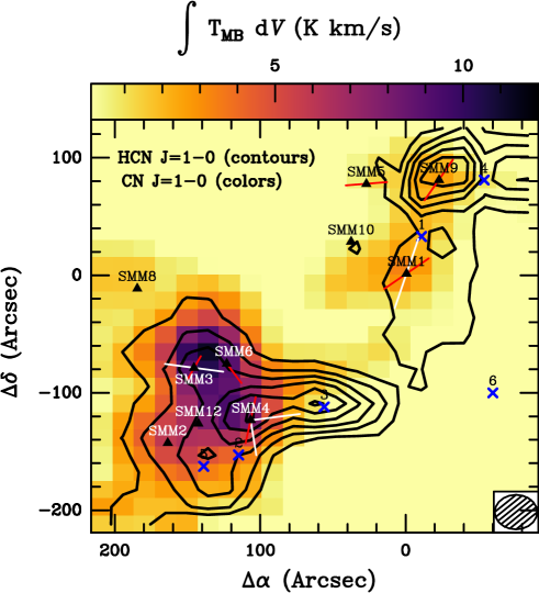
Figure 10: Map of CN 1-0 (colors) and HCN 1-0 (contours) in the Serpens Main. The labels are the same as in Figure 2. Contour levels start at 8 K km s^-1 with the steps of 3 K km s^-1. The CN emission has been resampled to the beam size of HCN to compare the same emitting regions.

Yıldız et al. (2015) used ¹³CO 6-5 emission as an alternative way to quantify the spatial extent of UV radiation for a sample of $\sim 30$ Class 0/I protostars. They isolated a narrow component of the line profiles attributed to the UV-heated gas, in excess of envelope emission. The gas affected by UV was found to be aligned with the outflow direction on spatial scales of $\sim$1000-2000 AU, consistent with the extent of the CN/HCN enhancement. The elongated pattern of ¹³CO 6-5 was more clearly detected in Class 0 sources, but the total amount of gas affected by the UV radiation was not found to be correlated with the evolutionary stage.

Figure 11 shows the CN/HCN luminosity ratio as a function of $T_{\mathrm{bol}}$ and $L_{\mathrm{bol}}$ for all protostars observed in the Serpens Main. The strength of the correlations is quantified using the Pearson coefficient, $r$, where for the sample of 10 protostars $|r|$ of 0.33, 0.67, and 1 corresponds to a 1$\sigma$, 2$\sigma$, and $3\sigma$ correlation, respectively. Clearly, the Pearson coefficients of 0.3-0.4 indicate a lack of any correlation that would suggest evolutionary changes in the CN/HCN emission during the Class 0/I phases. It is consistent with a lack of significant changes in the [O I] line emission from Class 0 to Class I in a sample of about 90 protostars observed with Herschel/PACS, which is also connected with the amount of UV radiation (Karska et al., 2018).

The spatial extent of CN and HCN emission implies that UV photons are wide-spread in the Serpens Main region on cluster scales. The enhancement of the CN/HCN ratio is associated with the parts of outflows mostly affected by UV from protostars and does not depend on the evolutionary stage. The changes in the spatial patterns of CN and HCN with evolution on small scales would require higher spatial resolution observations.

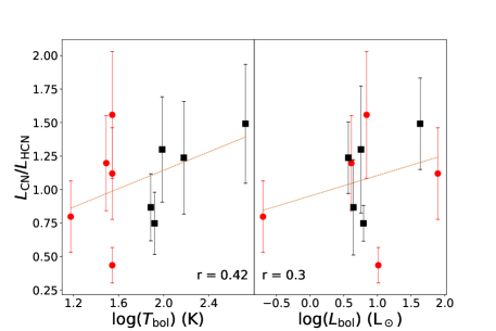
Figure 11: Correlations of line luminosity ratios with bolometric temperature and luminosity of protostars. Class 0 protostars are marked with red dots, while Class I with black squares. The Pearson coefficient of the correlation (r) is shown.

5.2 Chemical effects

In the presence of strong UV radiation, HCN photodissociates into CN and H, while CN requires even more energetic photons (¿12.4 eV) to be dissociated (van Dishoeck 1987). This should lead to a higher abundance of CN molecules and an increase of the CN/HCN column density ratio. Despite many limitations and approximations, the chemical model presented in Section 4 demonstrates that the CN/HCN ratio is sensitive to the UV field. The strength of UV radiation distinguishes the dominant reactions. The density and temperature have less effect on chemistry, at least below a few hundred K. Three regimes can be defined: weak (G₀ ¡ $10^{-1}$), intermediate (G${}_{0}\sim 10^{-1}-10^{1}$) and strong (G₀ ¿ $10^{1}$) UV field. They correspond to regimes where the bulk of carbon is either in the molecular (CO), atomic (C), or ionized (C⁺) form, which has a significant impact on chemical networks.

In starless, dark, non-turbulent clouds, HCN is more abundant than CN by about an order of magnitude (Pratap et al. 1997). This is in agreement with our model of a starless cloud after $10^{5}-10^{6}$ yr of cloud evolution (Figure 6). With the further chemical evolution of a starless cloud, the CN/HCN ratio decreases. In a weak UV field, the chemistry is similar to the star-less, dark, non-turbulent interstellar cloud. Dominant formation channels of CN and HCN are reactions of nitrogen with hydrocarbons (CH and CH₂, respectively), while destruction of CN is mostly dominated by the reactions with neutral oxygen or nitrogen. HCN is less reactive than CN, and reactions with neutral atoms are not very efficient in this case. Many reaction channels drive the destruction of HCN, but reactants are less abundant than neutral atoms. The simultaneous impact of a few different reactions is not as effective as the reaction ruling the CN destruction. Those factors lead to the higher HCN abundances compared to CN.

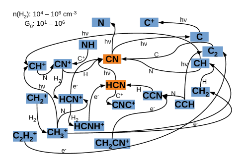
Figure 12: Reaction network predicted by the Nahoon model assuming the UV field strength is higher than 10 G₀. The dominant reactions are listed in Table  4

.

As the intensity of UV radiation increases, photodissociation and photoionization become more important. For strong radiation field, the destruction of CN is dominated by reaction: CN -¿[UV photons] C +N.
However, at intermediate UV field strength, photodissociation of CN is not efficient and the reaction with neutral oxygen is important:
CN + O -¿ N + CO.
For intermediate and strong radiation fields, C+ is significantly more abundant than C. It opens a very effective channel of HCN destruction:
C -¿[UV photons] C+ + e-
HCN + C+ -¿ H + CNC+
CNC+ + e- -¿ CN + C
The presence of this channel leads to a significantly lower concentration of HCN than CN for intermediate UV fields. The HCN molecule can be destroyed directly by UV photons:
HCN -¿[UV photons] H + CN.
This reaction is dominant for the strong UV fields. Nevertheless, the exact balance between the two ways of destroying HCN depends on temperature and density.

The CN/HCN ratio can also be shaped by several factors neglected in the chemical model, including grain chemistry, evaporation, turbulence, shocks, the spectrum of UV emission of a particular object. Ice chemistry, as well as grain sublimation, can significantly alter the results. Although not yet detected in the ISM (Boogert et al., 2015), HCN is postulated to exist in the interstellar ice with the abundance of $10^{-8}$ relative to hydrogen (Kalvāns, 2015). Thus, HCN can sublimate under the influence of increasing temperature or UV light, leading to a decrease in the CN/HCN ratio. CN may be also produced by the photodegradation and photoevaporation of CN-bearing complex organic molecules trapped in ice. Even though a high CN reactivity causes it to be present at a low concentration in interstellar ice and dust, thermal degradation of CN-bearing dust may be an important CN source, as postulated for comets (Hänni et al. 2020; Lippi, M. et al. 2013).

Finally, European Space Agency’s Rosetta spacecraft, measured a higher concentration of HCN than CN in the comet 67P/Churyumov–Gerasimenko (Hänni et al. 2020). Considering that the chemistry of N-bearing species in 67P/C-G is similar to interstellar ice chemistry (Jørgensen et al., 2020), we expect that the CN/HCN ratio predicted by the presented chemical model is slightly overestimated.

5.3 UV field strengths in the Serpens Main

Observations of CN and HCN elucidate the presence of UV fields in the immediate surroundings of low- and intermediate-mass protostars. To determine the strengths of the UV fields, we calculated chemical models to reproduce the observed column density ratios.

The measured CN/HCN ratios are consistent with the chemical models that include UV radiation, and for a broad range of physical conditions typical for low-mass star-forming regions. The UV field strengths, G₀, in excess of 10³ best reproduce the observed CN/HCN ratios assuming gas temperature of 50 K (Section 3.2). At a gas temperatures of 300 K, the CN/HCN ratio is consistent with UV fields of 0.1-10 (Fig. 21). In both regimes, the dominant destruction reaction of HCN is indeed the photodissociation by UV photons.

An alternative measure of the UV fields around protostars was recently provided by the observations of H₂O as part of the WISH program on Herschel (van Dishoeck et al., 2021). Far-infrared molecular spectra indicate that the bulk of H₂O forms in non-dissociative shocks in outflows at gas temperature $\sim$300 K (Herczeg et al., 2012; Green et al., 2016; Karska et al., 2018). Some H₂O emission arises in hotter, $T\gtrsim 700$ K regions with enhanced emission from hydrides, e.g. OH⁺, where dissociative shocks are at play (Kristensen et al., 2013). The fraction of H₂O in the outflows is clearly photodissociated, as evidenced by low absolute abundances and unexpectedly bright emission of OH and O (Wampfler et al., 2013; Kristensen et al., 2017). The impact of UV photons on non-dissociative shocks was modeled by Melnick & Kaufman (2015). The models reproduced the observed ratios of H₂O/OH and CO/OH in low-mass protostars for UV fields with G₀ of 0.1-10 (Karska et al., 2018). The same ratios showed a few orders of magnitude disagreement with fully-shielded shock models, providing further evidence for H₂O photodissociation (Karska et al. 2014).

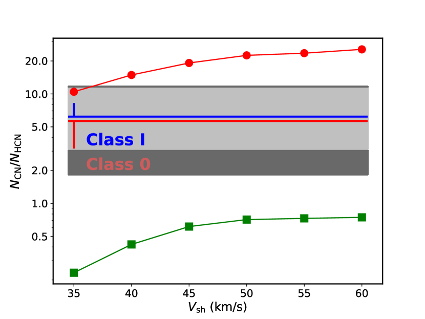
Figure 13: The observed CN/HCN column density ratio compared with shock models with UV for a preshock density of $10^{4}$ cm^-3 (Lehmann et al., 2020). The column densities are shown as a function of shock velocity for the precursor and post-shock regions (in red circles), and the postshock region alone (in green squares). Column densities ratios obtained for Class 0 and Class I protostars are shown with dark grey and light grey rectangles, respectively. The horizontal lines show median CN/HCN ratios, and the vertical lines - their standard deviations for Class 0 (red) and Class I (blue) sources, respectively

.

The spectrum of the UV radiation adopted in Melnick & Kaufman (2015) is based on average interstellar measurements, and is best suited for modeling the external irradiation. The spatial extent of the enhanced CN/HCN ratio and ¹³CO 6-5 emission suggest that UV photons in most protostars are likely produced in-situ, in the immediate surrounding of the outflow shocks (see Section 5.1, Yıldız et al., 2015). Recent models by Lehmann et al. (2020) provide predictions for molecular abundances arising in shocks where UV emission originates from the shock itself, i.e. the self-generated UV radiation. The calculations are done for a single gas pre-shock density of 10⁴ cm^-3, which corresponds to (post-shock) gas densities of $\sim$10⁶ cm^-3, assuming a compression factor of 100 typical for dissociative shocks. The UV fields generated by shocks with velocities in the range from 35 to 60 km s^-1 are $\sim 10-400$ larger than the interstellar radiation field. In this regime, CN/HCN$>1$ when considering the entire shock region; CN/HCN$<1$ for lower-velocity shocks and the postshock region alone (see Figure 13).

Observations of CN and HCN in the Serpens Main are consistent with the Lehmann et al. (2020) shock models with velocities of 35 km s^-1, but only for the regions with the highest CN/HCN ratios (Figure 13). These shocks produce UV fields $G_{\mathrm{eff}}\sim 25$, where $G_{\mathrm{eff}}$ is the flux of UV photons normalized to the average interstellar UV field (Lehmann et al., 2020), and have a relatively short lifetime of $\sim 10^{3}$ yrs. The UV fields are lower than G₀ of $\sim 10^{3}$ predicted by the chemical model with UV (Section 4), which could be due to many different factors and assumptions. In particular, neither of the models reproduces the physical structure of the protostellar envelope with outflows.

The models of the CN/HCN ratio in the dense envelopes of high-mass protostars were pioneered by Stäuber et al. (2007), who considered both the effect of UV and X-ray radiation fields. The 1D radiative-transfer models accounted for the temperature and density gradients in the envelope, and the abundance profiles of the two molecules. The observed CN/HCN ratios in the envelopes were well-reproduced with $G_{0}<100$ at $T_{\mathrm{gas}}\gtrsim 200$ K, and densities of 10⁶ cm^-3. For lower gas temperatures, radiation from X-ray photons was invoked to explain the observations.

Bruderer et al. (2009b) extended the 1D models by carving out a low-density outflow region in the envelope, which allowed a more efficient irradiation. The introduction of outflow cavity walls facilitated a significant increase in the volume of FUV irradiated gas. An example 2D model of AFGL 2591 successfully reproduced the CO⁺ emission at $G_{0}>10^{2}$ (Bruderer et al., 2009a).

Recent observations of additional hydrides provide further estimates of the radiation fields in high-mass protostars. Benz et al. (2016) used new envelope models including outflow cavities to reproduce the abundances of e.g. CH⁺, OH⁺ and H₂O⁺. The UV fields of 20-600 times the average interstellar radiation field were invoked to reproduce the observations of high-mass protostars. Lower UV fields, 2-400 times the interstellar radiation field, were found for low-mass protostars. The impact of X-ray photons on the chemistry was not observed in the envelopes. For gas densities of 10⁶ cm^-3, the ratios of $\sim 1-12$ observed in the Serpens Main are consistent with the models of Stäuber et al. (2007) with $G_{0}\lesssim 10^{2}$ and gas temperatures $\gtrsim 300$ K. Inclusion of the lower-density outflow cavities similar to Benz et al. (2016), would better reproduce the CN/HCN ratios due to easier propagation of UV photons at lower densities. Such a modeling, however, is outside of the scope of this paper.

In summary, the CN/HCN ratio provides information about UV field distribution on cluster scales. Independent measurements of gas densities allow the estimate of the strengths of the UV fields. Their values in the surrounding of low-mass protostars in Serpens are of the order of $10^{3-4}$ the interstellar radiation field, qualitatively in agreement with observations and modeling of other species. While opacity effects influence the results of calculations, UV fields clearly play a significant role even around Solar-type protostars and affect the chemistry and physical properties of material in the forming disks (Visser et al. 2009, Drozdovskaya et al. 2016).

6 Conclusions

IRAM 30 m / EMIR observations of CN and HCN emission pin-point the location of the impact of UV radiation on the chemistry of low-mass star forming region in the Serpens Main. A combination of simple models using the radiative transfer code RADEX and the chemical code Nahoon allows us to determine physical conditions of the gas, column densities of molecular species, and estimate the UV radiation field strength. The main conclusions of our study are the following:

• The large-scale spatial extent of HCN and CN emission show differences, with HCN resembling more the CO emission tracing outflows and CN concentrated closer to the individual protostar positions. Yet, on spatial scales on individual sources, both tracers are associated with outflows.

• Analysis of the ratios of hyperfine-splitted components shows that HCN 1-0 and H¹³CN 1-0 are optically thick, and CN 1-0 is typically optically thin. Thus, the opacity effects influence the spatial distribution of CN/HCN enhancements by underestimating HCN emission and overestimating the ratio of CN and HCN in dense regions. Column densities of HCN corrected for optical depth and determined from a simple scaling of H¹³CN agree within a factor of 2.

• For typical physical conditions of the gas in low-mass star forming regions column density ratio of CN and HCN is in the range of 1–12. For gas temperatures below $\sim 200$ K, derived UV field strengths are weakly dependent on the assumed gas densities in the models. At higher gas temperatures, the CN/HCN ratios are also consistent with lower UV fields, in line with measurements obtained using hydrides with Herschel (Benz et al., 2016).

• Enhancements of the CN/HCN ratios trace UV field strengths in excess of 10³ times the interstellar UV field toward the analyzed protostars and off-source positions in Serpens Main. Adopting measurements of gas densities at 1000 AU in the low-mass envelopes from Kristensen et al. (2012), G₀ of $\sim 10^{3}-10^{4}$ is inferred toward Ser SMM1, SMM3, and SMM4.

• The chemical network for nitrogen-bearing species is sensitive to UV photons. The CN/HCN ratio is primarily driven by the destruction of HCN by UV radiation field for G${}_{0}>10^{2}$ in the immediate surroundings of low-mass protostars.

• The luminosity ratio of CN and HCN toward low- and intermediate protostars in Serpens is not correlated with bolometric temperature and luminosity, suggesting a similar amount of UV photons affecting the gas. This results is consistent with far-infrared observations of [O I] toward a larger sample of sources, where no significant changes have been seen between Class 0 and Class I low-mass protostars (Karska et al., 2018).

The CN/HCN ratio as a tracer of the UV field can now be - with all the limitations - extended to the low-mass regime. Higher resolution observations are needed to fully exploit the impact of UV radiation on the low-mass star forming regions on scales of individual objects. Detailed 3D modeling of protostellar envelopes with outflow cavities is necessary to fully constrain the strengths of the UV fields in physical components of young stellar objects.

Appendix A Spectral Energy Distributions

Broad-band observations are needed in order to determine physical properties of a protostar. Dunham et al. (2015) studied protostars in the Serpens molecular cloud using 2MASS (Skrutskie et al. 2006) and Spitzer IRAC/MIPS (Evans et al. 2009) observations covering the range 1.25–70 $\mu$m, photometry from Wide-field Infrared Survey Explorer at 12 and 22 $\mu$m (WISE; Wright et al. 2010), SHARC-II 350 $\mu$m (Suresh et al. 2016), the SCUBA Legacy Catalog 450 and 850 $\mu$m (Di Francesco et al. 2008) and 1.1 mm observations from Bolocam dust survey (Enoch et al. 2007). The Serpens Main region was also observed in the Herschel Gould Belt survey project (André et al. 2010) at 70, 160, 250, 350 and 500 $\mu$m. SPIRE/PACS photometry in the Serpens molecular cloud is discussed in Fiorellino et al. (2021). The flux densities used in the analysis are shown in Table 6.

Table 5: Comparison of $T_{\mathrm{bol}}$ and $L_{\mathrm{bol}}$ with literature values

Source	$T_{\mathrm{bol}}$	$T_{\mathrm{bol}}$ (reference)	$L_{\mathrm{bol}}$	$L_{\mathrm{bol}}$ (reference)	Difference
	(K)	(K)	(L⊙)	(L⊙)	%
SMM 1	37	39 (1)	115.2	108.7 (1)	-5	+6
SMM 2	34	28 (2)	7.2	8.0 (2)	+21	-10
SMM 3	35	37 (1)	7.1	27.5 (1)	-5	-74
SMM 4	68	28 (1)	5.1	13.6 (1)	+143	-63
SMM 5	151	130 (2)	3.7	4.8 (2)	+16	-23
SMM 6	532	530 (2)	43.1	42.0 (2)	+0.4	+3
SMM 8	15	…	0.2	…	–	–
SMM 9	33	29 (2)	11.0	14.0 (2)	+14	-21
SMM 10	79	62 (2)	7.1	7.6 (2)	+27	-7
SMM 12	72	100 (2)	10.0	6.2 (2)	-28	+61

Table 6: Continuum fluxes in Jy

$\lambda$	SMM1	SMM2	SMM3	SMM4	SMM5	SMM6	SMM9	SMM10	SMM12
($\mu$m)
1.25	-	-	-	6.0$\times$10-4	3.0$\times$10-4	2.1$\times$10-2	-	-	-
1.65	-	-	-	3.2$\times$10-3	9.0$\times$10-4	2.1$\times$10-1	-	-	-
2.17	-	-	-	1.0$\times$10-2	4.3$\times$10-3	1.0$\times$100	-	-	-
3.6	9.0$\times$10-4	4.0$\times$10-4	2.8$\times$10-3	2.4$\times$10-2	3.1$\times$10-2	2.5$\times$100	2.0$\times$10-3	7.4$\times$10-3	2.8$\times$10-3
4.5	2.6$\times$10-3	1.2$\times$10-3	5.8$\times$10-3	3.3$\times$10-2	7.3$\times$10-2	3.0$\times$100	7.0$\times$10-3	3.3$\times$10-2	3.0$\times$10-2
5.8	2.3$\times$10-3	2.1$\times$10-3	7.8$\times$10-3	4.1$\times$10-2	1.4$\times$10-1	5.1$\times$100	1.2$\times$10-2	4.1$\times$10-2	1.0$\times$10-1
8	3.5$\times$10-3	3.5$\times$10-3	3.6$\times$10-2	5.6$\times$10-2	2.1$\times$10-1	5.4$\times$100	1.7$\times$10-2	-	2.0$\times$10-1
12	6.2$\times$10-3	-	-	-	1.8$\times$10-1	7.6$\times$100	1.2$\times$10-2	3.8$\times$10-2	2.2$\times$10-1
22	1.0$\times$100	-	-	-	9.5$\times$10-1	1.0$\times$101	2.1$\times$10-1	8.0$\times$10-1	3.1$\times$100
24	1.2$\times$100	1.0$\times$10-1	1.1$\times$10-1	2.8$\times$10-1	9.9$\times$10-1	-	2.2$\times$10-1	1.6$\times$100	2.6$\times$100
70	2.6$\times$102	1.1$\times$101	7.7$\times$100	1.9$\times$100	8.5$\times$100	2.6$\times$101	1.5$\times$101	8.8$\times$100	1.2$\times$101
160	5.8$\times$102	3.8$\times$101	4.2$\times$101	2.6$\times$101	1.8$\times$100	3.1$\times$101	6.1$\times$101	1.4$\times$101	4.3$\times$101
250	2.4$\times$102	3.1$\times$101	4.2$\times$101	5.9$\times$101	4.0$\times$100	2.9$\times$101	5.9$\times$101	6.9$\times$100	5.3$\times$101
350	1.2$\times$102	3.1$\times$101	3.5$\times$101	4.7$\times$101	1.6$\times$101	1.6$\times$101	4.3$\times$101	6.5$\times$100	2.7$\times$101
450	1.0$\times$102	-	3.1$\times$101	-	-	-	-	-	-
500	5.5$\times$101	1.8$\times$101	1.7$\times$101	2.9$\times$101	1.2$\times$101	9.5$\times$100	2.3$\times$101	5.1$\times$100	1.8$\times$101
850	1.5$\times$101	8.9$\times$100	8.9$\times$100	-	3.9$\times$100	-	1.3$\times$101	3.0$\times$100
1100	6.5$\times$100	2.1$\times$100	2.1$\times$100	-	1.5$\times$100	1.6$\times$100	3.0$\times$100	1.0$\times$100	2.1$\times$100

Based on Spectral Energy Distributions (SEDs), the bolometric temperature and luminosity can be calculated for each of the observed protostars. The bolometric luminosity is determined by integrating the SEDs over frequency:

$$L_{bol}=4\pi\,d^{2}\,\int F_{\nu}d\nu$$ (5)

where $d$ is the cloud distance of $436\pm 9.2$ pc (Ortiz-León et al. 2017). The bolometric temperature is calculated as described in Myers & Ladd (1993):

$$T_{bol}=1.25\,10^{-11}\,\bar{\nu}$$ (6)

where $\bar{\nu}$ is the mean frequency given by:

$$\bar{\nu}=\frac{\int\nu F_{\nu}d\nu}{\int F_{\nu}d\nu}$$ (7)

Using Scipy splrep and splev functions, cubic smooth spline interpolation of the photometric data is obtained while calculating the protostars parameters. Integration along the resulting axis is obtained with the composite trapezoidal rule (Scipy package). The photometric data allow us to perform the integration along a wide range of wavelengths (Tab. 6) with the exception of SMM 8. For this source we have only 4 photometric points from the Herschel Gould Belt survey so the calculated bolometric temperature and luminosity may be underestimated.

Table 5 shows bolometric temperatures and luminosities, and their comparison to the literature values from Karska et al. (2018) and Dunham et al. (2015). The differences are lower than 30% for most of the sources, with the exception of Ser SMM3, SMM4, and SMM 12 where $L_{\mathrm{bol}}$ differs by a factor of $\sim 2-4$. The differences are mostly driven by the far-infrared measurements: Karska et al. (2018) use PACS $5\times 5$ single footprint maps covering a field of view of 47”$\times$47” and the range from 55 to 190 $\mu$m, and Dunham et al. (2015) use significantly less sensitive Spitzer/MIPS photometry. Here, we use photometric bands at 70 $\mu$m, 100 $\mu$m and 160 $\mu$m from the Herschel Gould Belt survey, with the beam sizes of 5.6”, 6.8”, and 10.7”, respectively. For Ser SMM3, there is a factor of 5-6 difference in the flux density at 70 $\mu$m (7 Jy vs. 36 Jy) and 160 $\mu$m (44 Jy vs. 182 Jy) between the PACS photometry and the 47”$\times$47” from spectroscopy. Similarly, for Ser SMM4 the 160 $\mu$m flux differs by a factor of $\sim$6, suggesting that the large field-of-view of the spectroscopy mode might include some additional emission from background or nearby sources.

Appendix B Maps in additional tracers

IRAM 30m spectral line maps in HCN and CS isotopologues are presented in Figure 15 and Figure 16. The H¹³CN 1-0 emission is a sum of all hyperfine splitting components. The H¹³CN 1-0 is spatially consistent with HCN 1-0, although a few times weaker. It peaks around Ser SMM2, Ser SMM4 and Ser SMM9, as well as at the outflow position no. 3. Except for the Ser SMM2 protostar, the peaks in H¹³CN 1-0 are co-spatial with the HCN emission peaks. The emission of H¹³CN 1-0 line is similarly strong in the south-east and north-west regions of the map.

The C³⁴S 3-2 line does not show such extended emission, although it is detected in all outflow positions. The emission is concentrated mostly near Ser SMM1, Ser SMM4 and Ser SMM9 sources, unlike the CS 3-2 which is not that significant around Ser SMM1. The isotopologues trace the same gas as their regular counterparts.

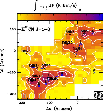
Figure 15: Similar to Figure 2 but for H¹³CN $1-0$. The first contour is at 3 $\sigma$ (0.5 K km s^-1) with steps of 3 $\sigma$

.

Figure 16: Similar to Figure 2 but for C³⁴S $3-2$. The first contour is at 3 $\sigma$ (1.2 K km s^-1), with steps of 1.5 $\sigma$.

Appendix C Line profiles across the maps

A majority of targeted lines are detected at protostar and outflow positions. Figures 17 and 18 show line profiles in CO 6-5 observed with APEX-CHAMP⁺ and C³⁴S 3-2, CS 3-2, H¹³CN 1-0, HCN 1-0 and CN 1-0 lines obtained with IRAM 30m. Note that the line profiles of Ser SMM4 and its outflow position are shown in Figure 3. The H¹³CN 2-1 line is detected only toward Ser SMM4 and Ser SMM9. The Ser SMM8 protostar is outside of the mapping area in CO 6-5.

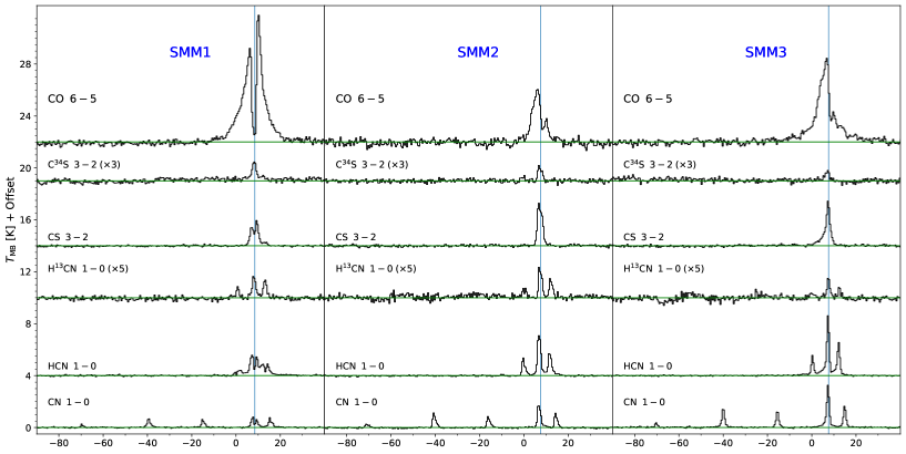
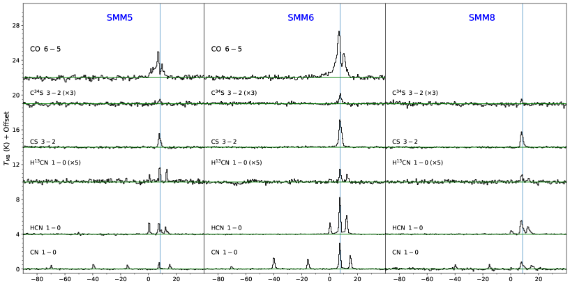
Figure 17: Line profiles of CO 6-5, C³⁴S 3-2, CS 3-2 , H¹³CN 2-1, H¹³CN 1-0, HCN 1-0 and CN 1-0 in the protostar positions.

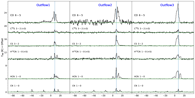
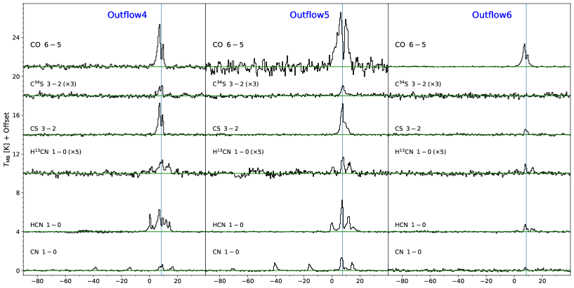
Figure 18: Line profiles of CO 6-5, C³⁴S 3-2, CS 3-2 , H¹³CN 2-1, H¹³CN 1-0, HCN 1-0 and CN 1-0 in the outflow positions.

Appendix D Line fluxes and observed column densities

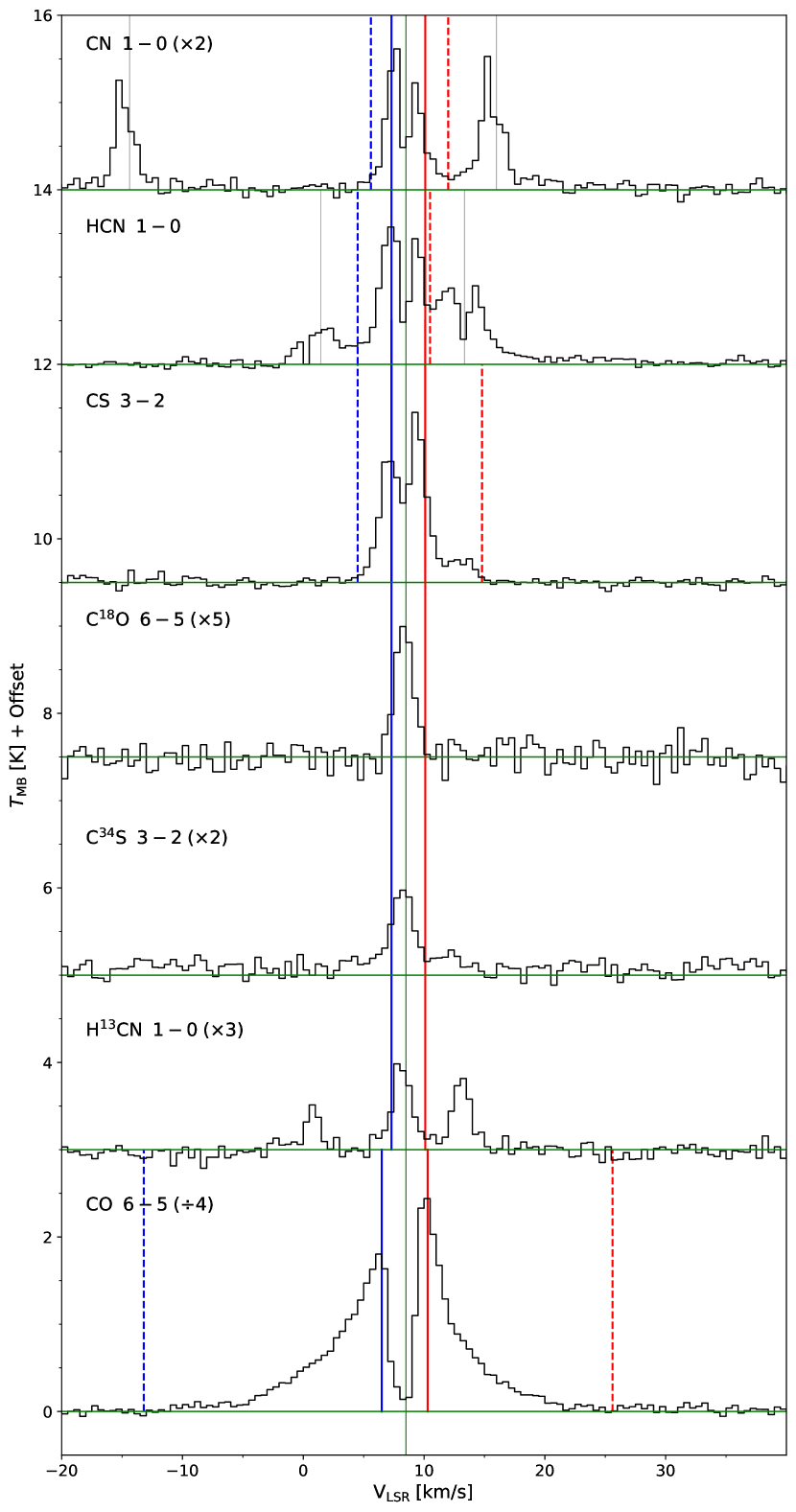
(a)

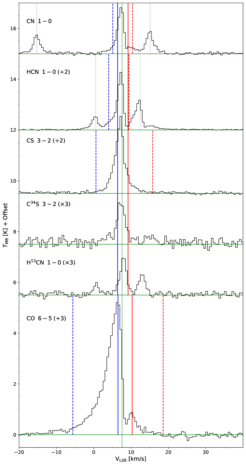
(b)

Figure 19: Line emission for Ser SMM1 (a) and SMM4 (b) with ranges for calculations of blue and red line wing emission. The C¹⁸O 6-5 line profile for Ser SMM1 is used as a proxy for the velocity range corresponding to the envelope emission (Kristensen et al. 2010).

Table 7: Velocity ranges (in km s${}^{-1})$ used to calculate emission in the line wings

Line	SMM 1		SMM 4
	blue	red	blue	red
CN 1-0	(-71.0,-70.0)	(-68.4,-68.1)	(-70.9, -70.9)	(-69.3, -68.7)
	(-42.2, -39.6)	(-38.0, -36.2)	(-41.6, -40.5)	(-38.9, -37.6)
	(-16.7, -15.1)	(-13.5, -13.0	(-19.2, -16.0)	(-14.4,-11.6)
	(5.6, 7.8)	(9.4, 12.0)	(5.1, 6.9)	(8.5, 10.4)
	(12.6, 15.3)	(16.9, 17.6)	(13.5, 14.4)	(16, 17.5)
HCN 1-0	(-1.3, 0.735)	(2.335, 3.5)	(-3.3, -0.2)	(1.4, 4.0)
	(4.5, 7.8)	(9.4, 10.5)	(4.0, 6.9)	(8.5, 9.4)
	(10.5, 12.64)	(14.24, 16)	(9.4, 11.7)	(13.3, 18.9)
CS 3-4	(4.5, 7.3)	(9.4, 14.8)	(0.6, 6.9)	(8.5, 15.8)
CO 6-5	(-11.3, 7.8)	(9.4, 21.7)	(-13.2, 6.9)	(8.5, 17.3)

Figure 19 shows line profiles in Ser SMM1 and SMM4 from IRAM 30m compared to the C¹⁸O line profile from APEX in order to select the velocity ranges for calculating emission in the line wings.

Table 7 shows the velocity ranges used to calculate integrated intensities in the line wings for each of the species. The extent of the line wings, $V_{\mathrm{out}}$, corresponds to the velocity range where the emission exceeds 2$\sigma$. The inner boundaries of the line wings are calculated using the C¹⁸O 6-5 line, with $V_{\mathrm{in}}$ corresponding to the velocity where the C¹⁸O emission drops below the 3$\sigma$ level in Ser SMM1 (Figure 19). The adopted ranges have been visually inspected to contain the entire wing emission and omit absorption at the line centers.

Table 8 shows line fluxes and level-specific column densities calculated at protostar positions. The integrated intensity is measured at 3$\sigma$ level for each spectrum separately. The peak temperature $T_{\mathrm{peak}}$ corresponds to the line maximum or to the maximum of the strongest hyperfine component. The uncertainties in $T_{\mathrm{peak}}$ are rms values calculated using the baseline in the vicinity of each line. Column densities at the upper lever $N_{\mathrm{up}}$ are calculated as described in Section 4.1 (Equation 2).

Table 9 shows total column densities $N_{\mathrm{tot}}$ calculated for total line profiles and wings separately (Equation 3) assuming $T_{\mathrm{exc}}=50$ K. The values are corrected using the optical depth correction factor $C_{\mathrm{\tau}}$ (Goldsmith & Langer 1999) defined as:

$$C_{\mathrm{\tau}}=\frac{\tau}{1-\exp^{-\tau}}$$ (8)

where $\tau$ is the optical depth.

Table 10 shows a comparison of HCN column densities calculated using corrections for optical depth and using scaled H¹³CN 1-0 column densities. Optical depths are calculated using the ratio of the hyperfine-splitted components, the F=2$\rightarrow 1\div$1$\rightarrow 1$ ($N$(HCN)${}_{\tau_{1}}$), and using Equation 1 (see Section 3.3.1) for the full line profile of HCN ($N$(HCN)${}_{\tau_{2}}$). The H¹³CN 1-0 column density is multiplied by a factor of 68 corresponding to the standard interstellar ¹²C/¹³C ratio (Milam et al. 2005). The mean ratios of column densities determined using H¹³CN 1-0 scaling and HCN corrected for optical depth, $N$(HCN)${}_{\tau_{1}}$ and $N$(HCN)${}_{\tau_{2}}$, is 0.7 and 2.1, respectively. Thus, the HCN column densities calculated using these methods agree within a factor of $\sim$2.

Table 8: Integrated fluxes and level-specific column densities at the positions of protostars

Line		SMM1	SMM2	SMM3	SMM4	SMM5	SMM6	SMM8	SMM9	SMM10	SMM12
CN 1-0	$\int{T_{\mathrm{mb}}\,dV}$	6.3 $\pm$ 0.9	8.5 $\pm$ 1.3	12.2 $\pm$ 1.8	10.2 $\pm$ 1.5	2.7 $\pm$ 0.4	10.6 $\pm$ 1.6	3.0 $\pm$ 0.5	4.9 $\pm$ 0.8	3.0 $\pm$ 0.5	10.1 $\pm$ 1.5
	(K km s-1)
	$T_{\mathrm{peak}}$ (K)	0.89 $\pm$ 0.03	1.92 $\pm$ 0.04	3.42 $\pm$ 0.03	1.90 $\pm$ 0.03	0.94 $\pm$ 0.04	3.17 $\pm$ 0.03	0.94 $\pm$ 0.13	0.84 $\pm$ 0.04	0.78 $\pm$ 0.03	1.85 $\pm$ 0.03
	$N_{\mathrm{up}}$ (cm-2)	1.30($\pm$0.07) $\times$1013	1.74($\pm$0.09) $\times$1013	2.50($\pm$0.13) $\times$1013	2.11($\pm$0.11) $\times$1013	5.17($\pm$0.03) $\times$1012	2.21($\pm$0.11) $\times$1013	6.22($\pm$0.04) $\times$1012	1.00($\pm$0.05) $\times$1013	6.25($\pm$0.03) $\times$1012	2.08($\pm$0.10 )$\times$1013
HCN 1-0	$\int{T_{\mathrm{mb}}\,dV}$	10.3 $\pm$ 1.6	13.1 $\pm$ 1.9	14.4 $\pm$ 2.2	21.7 $\pm$ 3.0	4.0 $\pm$ 0.8	13.1 $\pm$ 1.9	6.8 $\pm$ 1.1	20.7 $\pm$ 3.1	7.3 $\pm$ 1.1	14.2 $\pm$ 2.2
	(K km s-1)
	$T_{\mathrm{peak}}$ (K)	1.76 $\pm$ 0.04	3.48 $\pm$ 0.03	4.95 $\pm$ 0.03	4.69 $\pm$ 0.03	1.72 $\pm$ 0.04	5.15 $\pm$ 0.03	1.72 $\pm$ 0.04	2.40 $\pm$ 0.05	1.75 $\pm$ 0.03	3.50 $\pm$ 0.04
	$N_{\mathrm{up}}$ (cm-2)	6.49($\pm$0.33) $\times$1012	8.26($\pm$0.40) $\times$1012	9.17($\pm$0.47) $\times$1012	1.35($\pm$0.06) $\times$1013	2.58($\pm$0.16) $\times$1012	8.29($\pm$0.40) $\times$1012	4.33($\pm$0.23) $\times$1012	1.28($\pm$0.05) $\times$1013	4.58($\pm$0.23) $\times$1012	9.07($\pm$0.46) $\times$1012
CS 3-2	$\int{T_{\mathrm{mb}}\,dV}$	5.9 $\pm$ 1.1	8.6 $\pm$ 1.4	8.3 $\pm$ 1.6	14.8 $\pm$ 3.1	2.6 $\pm$ 0.5	8.5 $\pm$ 1.3	4.5 $\pm$ 0.7	12.4 $\pm$ 2.5	3.6 $\pm$ 0.8	9.9 $\pm$ 1.5
	(K km s-1)
	$T_{\mathrm{peak}}$ (K)	1.57 $\pm$ 0.05	3.10 $\pm$ 0.06	2.90 $\pm$ 0.06	4.30 $\pm$ 0.06	1.48 $\pm$ 0.06	3.2 $\pm$ 0.05	2.08 $\pm$ 0.05	2.70 $\pm$ 0.07	1.43 $\pm$ 0.05	3.26 $\pm$ 0.04
	$N_{\mathrm{up}}$ (cm-2)	4.06($\pm$0.11) $\times$1012	5.88($\pm$0.14) $\times$1012	5.72($\pm$0.15) $\times$1012	1.17($\pm$0.03) $\times$1013	1.87($\pm$0.05) $\times$1012	5.86($\pm$0.13) $\times$1012	3.07($\pm$0.07) $\times$1012	8.59($\pm$0.24) $\times$1012	2.47($\pm$0.08) $\times$1012	6.83($\pm$0.15) $\times$1012
C34S 3-2	$\int{T_{\mathrm{mb}}\,dV}$	1.3 $\pm$ 0.3	0.9 $\pm$ 0.2	0.5 $\pm$ 0.1	1.5 $\pm$ 0.3	0.3 $\pm$ 0.1	0.8 $\pm$ 0.2	0.3 $\pm$ 0.1	1.8 $\pm$ 0.3	0.4 $\pm$ 0.1	0.6 $\pm$ 0.1
	(K km s-1)
	$T_{\mathrm{peak}}$ (K)	0.56 $\pm$ 0.05	0.47 $\pm$ 0.04	0.36 $\pm$ 0.04	0.64 $\pm$ 0.05	0.42 $\pm$ 0.05	0.56 $\pm$ 0.03	0.35 $\pm$ 0.05	0.62 $\pm$ 0.04	0.40 $\pm$ 0.04	0.42 $\pm$ 0.05
	$N_{\mathrm{up}}$ (cm-2)	7.03($\pm$0.20) $\times$1011	4.75($\pm$0.14) $\times$1011	2.73($\pm$0.10) $\times$1011	8.29($\pm$0.22) $\times$1011	1.83($\pm$0.08) $\times$1011	4.23($\pm$0.12) $\times$1011	1.41($\pm$0.07) $\times$1011	1.02($\pm$0.03) $\times$1012	2.16($\pm$0.10) $\times$1011	3.17($\pm$0.10) $\times$1011
H13CN 1-0	$\int{T_{\mathrm{mb}}\,dV}$	1.6 $\pm$ 0.2	1.5 $\pm$ 0.2	0.6 $\pm$ 0.1	1.6 $\pm$ 0.3	0.8 $\pm$ 0.1	0.9 $\pm$ 0.1	0.1 $\pm$ 0.1	2.4 $\pm$ 0.3	1.0 $\pm$ 0.2	1.6 $\pm$ 0.3
	(K km s-1)
	$T_{\mathrm{peak}}$ (K)	0.45 $\pm$ 0.02	0.64 $\pm$ 0.02	0.41 $\pm$ 0.03	0.61 $\pm$ 0.03	0.42 $\pm$ 0.04	0.40 $\pm$ 0.02	0.21 $\pm$ 0.02	0.38 $\pm$ 0.03	0.45 $\pm$ 0.04	0.46 $\pm$ 0.03
	$N_{\mathrm{up}}$ (cm-2)	3.32($\pm$0.17) $\times$1011	3.08($\pm$0.15) $\times$1011	1.21($\pm$0.08) $\times$1011	3.41($\pm$0.18) $\times$1011	1.63($\pm$0.10) $\times$1011	1.82($\pm$0.08) $\times$1011	2.93($\pm$0.37) $\times$1010	5.01($\pm$0.22) $\times$1011	2.17($\pm$0.13) $\times$1011	3.43($\pm$0.18) $\times$1011
CO 6-5	$\int{T_{\mathrm{mb}}\,dV}$	75.6 $\pm$ 11.6	22.7 $\pm$ 3.7	52.5 $\pm$ 8.1	94.0 $\pm$ 14.3	13.1 $\pm$ 2.2	29.6 $\pm$ 4.6	-	36.2 $\pm$ 5.6	24.3 $\pm$ 3.9	17.3 $\pm$ 2.8
	(K km s-1)
	$T_{\mathrm{peak}}$ (K)	9.76 $\pm$ 0.18	4.04 $\pm$ 0.23	6.44 $\pm$ 0.17	15.61 $\pm$ 0.21	2.97 $\pm$ 0.17	5.33 $\pm$ 0.15	-	5.29 $\pm$ 0.12	3.76 $\pm$ 0.17	3.73 $\pm$ 0.18
	$N_{\mathrm{up}}$ (cm-2)	3.28($\pm$0.04) $\times$1015	9.83($\pm$0.12) $\times$1014	2.27($\pm$0.03) $\times$1015	4.07($\pm$0.05) $\times$1015	5.69($\pm$0.07) $\times$1014	1.28($\pm$0.02) $\times$1015	-	1.57($\pm$0.02) $\times$1015	1.07($\pm$0.01) $\times$1015	7.49($\pm$0.09) $\times$1015

Table 9: Column densities and corrected column densities calculated for the total flux and the wings

Line		SMM1	SMM2	SMM3	SMM4	SMM5	SMM6	SMM8	SMM9	SMM10	SMM12
CN 1-0	$N_{\mathrm{tot}}$ (cm-2)	1.38($\pm$0.17) $\times$1015	1.14($\pm$0.22) $\times$1015	1.47($\pm$0.32) $\times$1015	1.34($\pm$0.27) $\times$1015	6.28($\pm$0.72) $\times$1014	1.33($\pm$0.28) $\times$1015	3.74($\pm$0.92) $\times$1014	6.18($\pm$1.30) $\times$1014	7.52($\pm$0.81) $\times$1014	1.28($\pm$0.26) $\times$1015
	$N_{\mathrm{tot}}^{\mathrm{corr}}$ (cm-2)	1.14($\pm$0.17) $\times$1015	1.54($\pm$0.22) $\times$1015	2.17($\pm$0.32) $\times$1015	1.84($\pm$0.27) $\times$1015	4.68($\pm$0.72) $\times$1014	1.83($\pm$0.28) $\times$1015	5.12($\pm$0.92) $\times$1014	8.54($\pm$1.30) $\times$1014	5.05($\pm$0.81) $\times$1014	1.68($\pm$0.26) $\times$1015
	$N_{\mathrm{wings}}$ (cm-2)	4.93($\pm$0.11) $\times$1014	4.53($\pm$0.13) $\times$1014	2.94($\pm$0.12) $\times$1014	5.71($\pm$0.09) $\times$1014	5.90($\pm$1.40) $\times$1013	1.96($\pm$0.11) $\times$1014	1.09($\pm$0.24) $\times$1014	3.33($\pm$0.13) $\times$1014	1.02($\pm$0.12) $\times$1014	5.13($\pm$0.12) $\times$1014
	$N_{\mathrm{wings}}^{\mathrm{corr}}$ (cm-2)	1.25($\pm$0.01) $\times$1015	4.53($\pm$0.13) $\times$1014	2.94($\pm$0.12) $\times$1014	1.21($\pm$0.01) $\times$1015	5.90($\pm$1.40) $\times$1013	3.56($\pm$0.11) $\times$1014	1.09($\pm$0.24) $\times$1014	6.45($\pm$0.13) $\times$1014	1.02($\pm$0.12) $\times$1014	1.50($\pm$0.01) $\times$1015
HCN 1-0	$N_{\mathrm{tot}}$ (cm-2)	1.16($\pm$0.03) $\times$1015	1.14($\pm$0.03) $\times$1015	3.38($\pm$0.36) $\times$1014	1.24($\pm$0.05) $\times$1015	5.75($\pm$0.12) $\times$1014	6.45($\pm$0.31) $\times$1014	1.62($\pm$0.18) $\times$1014	1.81($\pm$0.04) $\times$1015	7.66($\pm$0.18) $\times$1014	1.15($\pm$0.04) $\times$1015
	$N_{\mathrm{tot}}^{\mathrm{corr}}$ (cm-2)	1.74($\pm$0.26) $\times$1014	2.10($\pm$0.31) $\times$1014	2.38($\pm$0.836) $\times$1014	3.56($\pm$0.49) $\times$1014	6.63($\pm$1.20) $\times$1013	2.24($\pm$0.31) $\times$1014	1.08($\pm$0.18) $\times$1014	3.40($\pm$0.51) $\times$1014	1.24($\pm$0.18) $\times$1014	2.33($\pm$0.36) $\times$1014
	$N_{\mathrm{wings}}$ (cm-2)	1.12($\pm$0.01) $\times$1014	8.31($\pm$0.10) $\times$1013	6.51($\pm$0.09) $\times$1013	1.40($\pm$0.01) $\times$1014	4.07($\pm$0.13) $\times$1013	4.34($\pm$0.09) $\times$1013	4.33($\pm$0.12) $\times$1013	2.62($\pm$0.02) $\times$1014	8.23($\pm$0.11) $\times$1013	1.03($\pm$0.01) $\times$1014
	$N_{\mathrm{wings}}^{\mathrm{corr}}$ (cm-2)	2.81($\pm$0.01) $\times$1014	8.29($\pm$0.10) $\times$1013	6.51($\pm$0.09) $\times$1013	2.95($\pm$0.01) $\times$1014	4.07($\pm$0.13) $\times$1013	7.76($\pm$0.09) $\times$1013	4.3(3$\pm$0.12) $\times$1013	4.95($\pm$0.02) $\times$1014	8.23($\pm$0.11) $\times$1013	2.94($\pm$0.01) $\times$1014
CS 3-2	$N_{\mathrm{tot}}$ (cm-2)	2.04($\pm$0.06) $\times$1014	1.31($\pm$0.08) $\times$1014	6.34($\pm$0.87) $\times$1013	2.31($\pm$0.17) $\times$1014	5.22($\pm$0.27) $\times$1013	1.22($\pm$0.07) $\times$1014	3.35($\pm$0.37) $\times$1013	2.94($\pm$0.14) $\times$1014	6.13($\pm$0.44) $\times$1013	7.54($\pm$0.84) $\times$1013
	$N_{\mathrm{tot}}^{\mathrm{corr}}$ (cm-2)	3.25($\pm$0.62) $\times$1013	4.76($\pm$0.81) $\times$1013	4.61($\pm$0.87) $\times$1013	8.32($\pm$1.70) $\times$1013	1.35($\pm$0.27) $\times$1013	4.84($\pm$0.74) $\times$1013	2.50($\pm$0.37) $\times$1013	7.01($\pm$1.40) $\times$1013	1.97($\pm$0.44) $\times$1013	5.49($\pm$0.84) $\times$1013
	$N_{\mathrm{wings}}$ (cm-2)	3.04($\pm$0.50) $\times$1013	2.06($\pm$0.07) $\times$1013	2.63($\pm$0.07) $\times$1013	6.07($\pm$0.07) $\times$1013	5.91($\pm$0.70) $\times$1012	1.82($\pm$0.06) $\times$1013	7.88($\pm$0.61) $\times$1012	7.89($\pm$0.08) $\times$1013	1.90($\pm$0.06) $\times$1013	2.16($\pm$0.05) $\times$1013
	$N_{\mathrm{wings}}^{\mathrm{corr}}$ (cm-2)	8.33($\pm$0.50) $\times$1013	4.12($\pm$0.07) $\times$1013	2.63($\pm$0.07) $\times$1013	1.14($\pm$0.01) $\times$1014	1.69($\pm$0.07) $\times$1013	1.82($\pm$0.06) $\times$1013	7.88($\pm$0.61) $\times$1012	1.74($\pm$0.01) $\times$1014	1.90($\pm$0.06) $\times$1013	4.41($\pm$0.05) $\times$1013

Table 10: Comparison of HCN column densities calculated from HCN 1-0 and H¹³CN 1-0 observations

Source	$N$(HCN)${}_{\tau_{1}}$	$N$(HCN)${}_{\mathrm{\tau_{2}}}$	$N$(H13CN)	Ratios
	hyperfine	full profile	$\times 68$
	1014 (cm-2)	1014 (cm-2)	1014 (cm-2)
SMM1	4.8($\pm$0.8)	1.7($\pm$0.3)	6.0($\pm$0.1)	1.3-3.5
SMM2	5.8($\pm$0.9)	2.1($\pm$0.3)	5.7($\pm$ 0.1)	1.0-2.7
SMM3	7.0($\pm$1.1)	2.4($\pm$0.8)	2.1($\pm$ 0.1)	0.3-0.9
SMM4	8.9($\pm$1.4)	3.6($\pm$0.5)	6.1($\pm$0.1)	0.7-1.7
SMM5	2.3($\pm$ 0.4)	0.7($\pm$0.1)	2.9($\pm$ 0.1)	1.3-4.1
SMM6	5.7($\pm$ 0.9)	2.2($\pm$0.3)	3.3($\pm$ 0.1)	0.6-1.5
SMM8	-	1.1($\pm$0.2)	0.5($\pm$ 0.1)	0.5
SMM9	-	3.4($\pm$0.5)	9.0($\pm$ 0.1)	2.6
SMM10	-	1.2($\pm$0.2)	3.9($\pm$ 0.1)	3.3
SMM12	7.5($\pm$ 1.1)	2.3($\pm$0.4)	6.1($\pm$ 0.1)	0.8-2.7

Appendix E Line ratios and optical depths

Table 11 shows line ratios of different species and Table 12 shows line ratios of different isotopologues of the same species. Figure 20 shows a corresponding correlation plots including the Pearson coefficient, $r$.

Table 13 shows optical depths of HCN and CS lines calculated using their rare isotopologues. Table 14 shows optical depths calculated using the ratios of hyperfine-splitted components for HCN, H¹³CN, and CN lines.

The Gaussian profiles were fitted to the hyperfine splitting components excluding wings with the PYSPECKIT package . The lines are blended at Ser SMM9, SMM10, and Outflow 4 positions, so the models cannot be fitted. Positive values of optical depths, $\tau>0$, are found when the following condition is met:

$$\frac{1-\exp(-\tau_{\mathrm{HCN}})}{\tau_{\mathrm{HCN}}}<1,$$ (9)

Both methods show that HCN is optically thick ($\tau_{\mathrm{HCN}}$¿1) in all positions. The median value of the optical depth for H¹³CN is $\sim 1$ and thus for some sources it is not optically thin. The exact values of $\tau_{\mathrm{HCN}}$ depend on the ratios which are used, which has been noted for other sources and referred to as hyperfine anomalies (Loughnane et al. 2012; Mullins et al. 2016). CN is optically thin toward most positions (except Ser SMM1, SMM5, and SMM10), and CS is optically thick in all positions except Ser SMM3 and SMM10, and off-position 3.

Table 11: Molecular line ratios of the fully integrated line profile and the line wings

Source	CN / HCN		CS / CO		HCN / CO
	Full	Line wings	Full	Line wings	Full	Line wings
Protostellar positions
Ser SMM1	0.61$\pm$0.10	0.40$\pm$0.08	0.08$\pm$0.01	0.05$\pm$0.01	0.14$\pm$0.02	0.10$\pm$0.02
Ser SMM2	0.65$\pm$0.10	0.53$\pm$0.15	0.38$\pm$0.06	0.23$\pm$0.05	0.58$\pm$0.09	0.35$\pm$0.07
Ser SMM3	0.85$\pm$0.13	0.57$\pm$0.11	0.16$\pm$0.03	0.10$\pm$0.03	0.27$\pm$0.04	0.10$\pm$0.02
Ser SMM4	0.47$\pm$0.08	0.40$\pm$0.08	0.16$\pm$0.03	0.12$\pm$0.03	0.23$\pm$0.03	0.13$\pm$0.03
Ser SMM5	0.67$\pm$0.09	0.31$\pm$0.06	0.19$\pm$0.04	0.09$\pm$0.03	0.31$\pm$0.06	0.17$\pm$0.06
Ser SMM6	0.81$\pm$0.13	0.55$\pm$0.11	0.29$\pm$0.04	0.19$\pm$0.03	0.44$\pm$0.07	0.14$\pm$0.03
Ser SMM8	0.43$\pm$0.07	0.27$\pm$0.04	-	-	-	-
Ser SMM9	0.24$\pm$0.04	0.11$\pm$0.02	0.34$\pm$0.07	0.30$\pm$0.06	0.57$\pm$0.09	0.49$\pm$0.06
Ser SMM10	0.41$\pm$0.06	0.15$\pm$0.03	0.14$\pm$0.03	0.09$\pm$0.03	0.29$\pm$0.04	0.23$\pm$0.04
Ser SMM12	0.71$\pm$0.10	0.63$\pm$0.10	0.57$\pm$0.08	0.40$\pm$0.05	0.82$\pm$0.13	0.49$\pm$0.10
Off-source positions
1 (-11.0,33.0)	0.58$\pm$0.09	0.24$\pm$0.04	0.24$\pm$0.03	0.15$\pm$0.02	0.43$\pm$0.07	0.31$\pm$0.04
2 (114.9,-153.0)	0.51$\pm$0.08	0.47$\pm$0.06	0.35$\pm$0.06	0.24$\pm$0.03	0.47$\pm$0.07	0.27$\pm$0.04
3 (56.0,-112.0)	0.13$\pm$0.02	0.03$\pm$0.01	0.54$\pm$0.09	0.56$\pm$0.16	0.74$\pm$0.13	0.72$\pm$0.20
4 (-54.0,81.0)	0.25$\pm$0.04	0.13$\pm$0.03	0.63$\pm$0.10	0.54$\pm$0.14	0.97$\pm$0.16	0.84$\pm$0.22
5 (138.9,-162.6)	0.56$\pm$0.09	0.49$\pm$0.09	0.26$\pm$0.04	0.18$\pm$0.03	0.36$\pm$0.06	0.21$\pm$0.03
6 (-60.0,-100.0)	0.35$\pm$0.08	0.16$\pm$0.10	0.38$\pm$0.04	0.16$\pm$0.04	0.59$\pm$0.06	0.49$\pm$0.05

Table 12: Molecular line ratios of the fully integrated line profile and the line wings using various isotopologues

Source	HCN / H13CN		CS / C34S	H13CN 2-1/1-0
	Full	Line wings	Full	Full
Protostellar positions
Ser SMM1	6.51$\pm$1.18	12.45$\pm$4.02	4.66$\pm$2.01	-
Ser SMM2	8.74$\pm$1.58	22.28$\pm$8.85	9.98$\pm$3.84	-
Ser SMM3	25.99$\pm$5.08	42.90$\pm$21.95	16.50$\pm$8.23	-
Ser SMM4	13.43$\pm$2.07	14.91$\pm$3.17	9.88$\pm$4.64	1.98$\pm$0.88
Ser SMM5	5.26$\pm$1.41	-	7.95$\pm$4.14	-
Ser SMM6	15.10$\pm$3.38	17.39$\pm$13.47	11.19$\pm$3.89	-
Ser SMM8	49.39$\pm$10.63	117.2$\pm$88.52	17.57$\pm$14.39	-
Ser SMM9	8.73$\pm$1.69	16.33$\pm$3.51	6.78$\pm$2.89	1.31$\pm$0.39
Ser SMM10	7.00$\pm$1.33	31.11$\pm$25.76	9.12$\pm$5.97	-
Ser SMM12	8.84$\pm$1.51	10.82$\pm$3.29	17.70$\pm$6.32	-
Off-source positions
1 (-11.0,33.0)	9.87$\pm$1.71	-	4.16$\pm$1.39	-
2 (114.9,-153.0)	13.48$\pm$2.18	27.12$\pm$12.16	10.71$\pm$3.53	-
3 (56.0,-112.0)	11.92$\pm$1.75	12.29$\pm$3.64	15.57$\pm$6.03	-
4 (-54.0,81.0)	8.38$\pm$1.41	12.12$\pm$2.78	8.90$\pm$3.18	-
5 (138.9,-162.6)	9.05$\pm$1.44	11.52$\pm$2.67	9.76$\pm$3.40	-
6 (-60.0,-100.0)	-	-	-	-

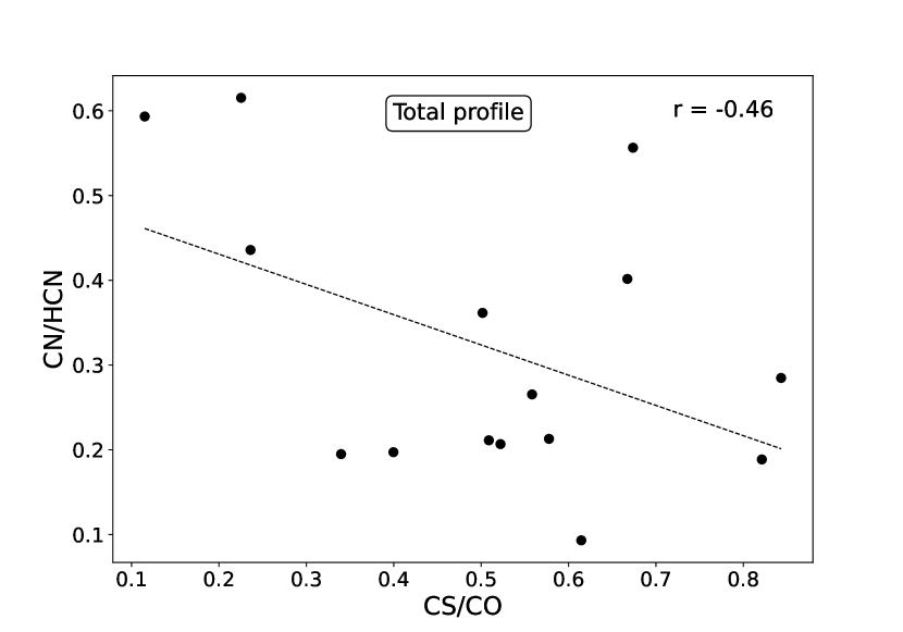
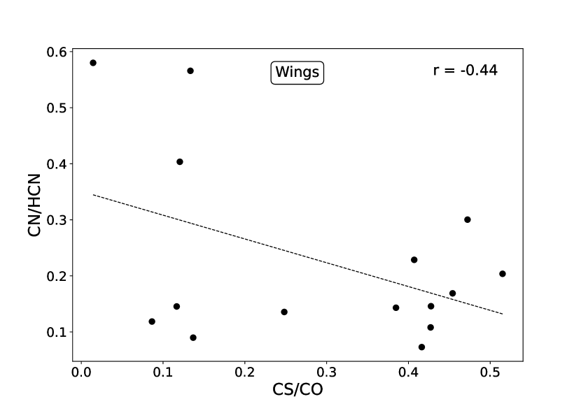
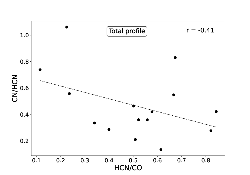
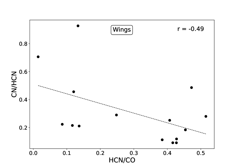
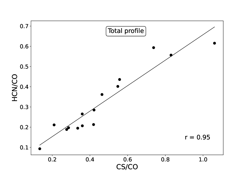
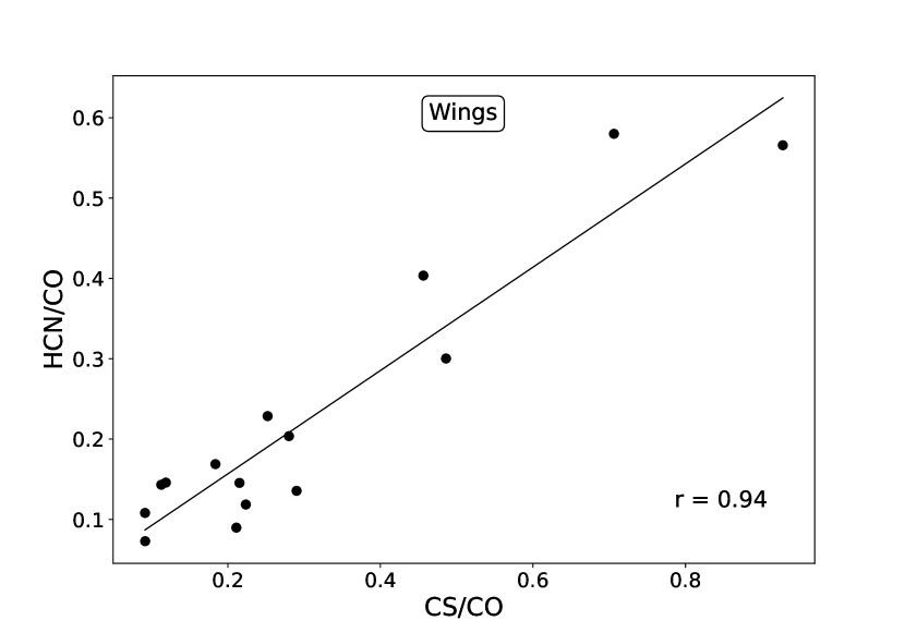
Figure 20: Correlations of the molecular line ratios of the fully integrated line profile (left panel) and the line wings (right panel) derived in protostellar and outflow positions. The Pearson coefficients ($r$) are shown on the plots; the number of datapoints is 15 in all cases. Solid lines show the best linear fits obtained with a least-squares method for cases where the Pearson coefficient exceeds the 3$\sigma$ threshold. Dashed lines show the fits for cases where the Pearson coefficient corresponds to 1.5-1.8$\sigma$ levels.

Table 13: Optical depths of line emission in HCN and CS for total profiles and line wings using rare isotopologues

Source	$\tau_{\mathrm{HCN}}$		$\tau_{\mathrm{CS}}$
	Full	Line wings	Full	Line wings
Protostar positions
Ser SMM1	10.31	2.12	4.39	2.56
Ser SMM2	7.60	0.63	1.69	1.53
Ser SMM3	2.33	–	0.47	–
Ser SMM4	4.96	1.61	1.71	1.42
Ser SMM5	12.80	–	2.35	2.66
Ser SMM6	4.38	1.21	1.39	0.89
Ser SMM9	7.72	1.37	2.88	1.86
Ser SMM10	7.69	–	1.94	–
Ser SMM12	9.61	2.56	0.32	1.59
Outflow positions
1 (-11.00,33.00)	6.80	–	4.91	5.63
2 (114.86,-153.00)	4.94	0.31	1.49	1.55
3 (56.00,-112.00)	5.60	2.32	0.59	0.46
4 (-54.00,81.00)	8.00	2.37	2.01	1.25
5 (138.86,-162.60)	7.40	2.53	1.74	1.77

Table 14: Optical depths of HCN, CN, and H¹³CN calculated using hyperfine-splitted components

Source	$\tau_{\mathrm{HCN}}$		$\tau_{\mathrm{H^{13}CN}}$		$\tau_{\mathrm{CN}}$
	F=2$\rightarrow$1 $\div$	F=1$\rightarrow$1 $\div$	F=2$\rightarrow$1 $\div$	F=1$\rightarrow$1 $\div$	F=5/2$\rightarrow$3/2 $\div$	F=5/2$\rightarrow$3/2 $\div$	F=1/2$\rightarrow$1/2 $\div$
	F=1$\rightarrow$1	F=0$\rightarrow$1	F=1$\rightarrow$1	F=0$\rightarrow$1	F=1/2$\rightarrow$1/2	F=3/2$\rightarrow$1/2	F=3/2$\rightarrow$1/2
Protostar positions
Ser SMM1	2.75	0.48	1.18	0.67	1.31	1.06	–
Ser SMM2	2.65	1.46	1.15	1.25	0.77	0.81	0.03
Ser SMM3	2.73	1.06	1.02	2.79	0.46	0.45	–
Ser SMM4	2.54	0.58	1.70	0.85	0.57	0.86	0.27
Ser SMM5	2.77	4.97	–	3.01	1.39	2.10	0.54
Ser SMM6	2.56	0.84	1.81	0.71	0.58	0.36	–
Ser SMM9	…	…	1.45	1.27	0.73	0.83	0.09
Ser SMM10	…	…	0.77	1.19	1.64	1.20	–
Ser SMM12	3.02	1.00	2.11	0.92	0.65	0.85	0.18
Outflow positions
1 (-11.00,33.00)	3.21	–	0.83	0.86	0.76	1.02	0.23
2 (114.86,-153.00)	2.66	0.34	2.76	–	0.34	0.16	–
3 (56.00,-112.00)	1.48	4.06	1.41	3.29	–	–	–
4 (-54.00,81.00)	…	…	0.88	1.32	0.84	0.64	–
5 (138.86,-162.60)	4.12	0.36	1.07	0.84	0.42	0.56	0.14

Appendix F Dominant reactions in CN, HCN chemistry

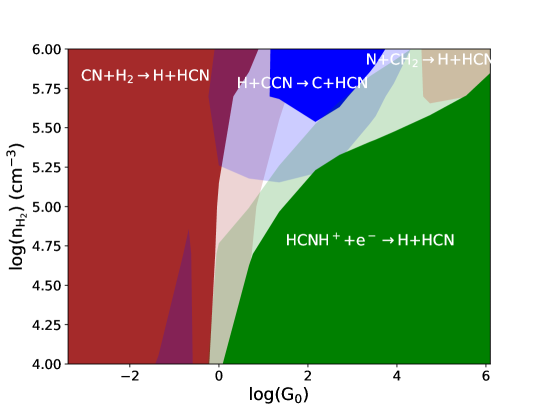
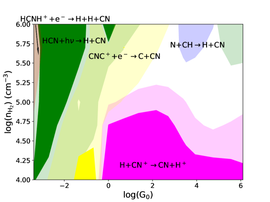
Figure 24: Similar to Figure 22 but for HCN (upper panel) and CN (bottom panel) production assuming $T\leavevmode\nobreak\ =\leavevmode\nobreak\ 300$ K. HCNH⁺ + e^- $\rightarrow$ H + HCN reaction is marked with green color, H + CCN $\rightarrow$ C + HCN with blue color, CN + H₂ $\rightarrow$ H + HCN with red color and N + CH₂ $\rightarrow$ H + HCN with orange. HCN + h$\nu$ $\rightarrow$ H + CN reaction is marked with green color, CNC⁺ + e^- $\rightarrow$ C + CN with yellow color, N + CH $\rightarrow$ H + CN with blue color and H + CN⁺ $\rightarrow$ CN + H⁺ with magenta.

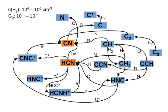
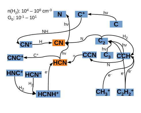
Figure 25: Reactions network for weakly and medium UV irradiated gas. The dominant reactions are listed in Table 4.

Dominant processes in CN and HCN reactions modeled at a temperature of 50 K and 300 K are listed in Table 4 and Table 15 respectively. The processes are illustrated in the Nahoon model parameter space: main channels of HCN and CN destruction (Figure 9 and Figure 22, as well as HCN and CN production (Figure 23 and Figure 24). Only the reactions contributing at least 30% in total flux are taken into consideration. Dominant reactions are more dependent on the strength of the UV radiation than on the hydrogen density, although in same cases the hydrogen density parameter plays role (See Tab. 15). Tab. 15 provides detailed information illustrated in Figure 9, Figure 22, Figure 23 and Figure 24. The weights of dominant reactions at each point of the calculated parameter space are presented as the percentage of the total flux. Reaction networks for UV radiation in weak (G₀ = $10^{-4}-10^{-1}$), intermediate (G₀ = $10^{-1}-10^{1}$) and strong (G₀ = $10^{1}-10^{6}$) regime are presented in Figure 25 and Figure 12. Not only the dominant reactions, but also the main route of the reactants production are illustrated.

Table 15: Dominant processes in CN and HCN chemistry at 300 K

Molecule	Weak UV fields	Medium UV fields	Strong UV fields
	(G0 = $10^{-3}-10^{-1})$	(G0 = $10^{-1}-10^{1})$	(G0 = $10^{1}-10^{6})$
CN	Destruction
	CN + H2 $\rightarrow$ H + HCN	O + CN $\rightarrow$ N + CO	CN + h$\nu$ $\rightarrow$ C + N
		CN + H2 $\rightarrow$ H + HCN	CN + H2 $\rightarrow$ H + HCN
		CN + h$\nu$ $\rightarrow$ C + N
	Production
	HCN + h$\nu$ $\rightarrow$ H + CN	CNC+ + e- $\rightarrow$ C + CN	H + CN+ $\rightarrow$ CN + H+
	CNC+ + e- $\rightarrow$ C + CN	H + CN+ $\rightarrow$ CN + H+	N + CH $\rightarrow$ H + CN
	HCNH+ + e- $\rightarrow$ H + H+ CN	HCN + h$\nu$ $\rightarrow$ H + CN	HCN + h$\nu$ $\rightarrow$ H + CN
HCN	Destruction
	HCN + h$\nu$ $\rightarrow$ H + CN	HCN + C+ $\rightarrow$ H + CNC+	HCN + h$\nu$ $\rightarrow$ H + CN
	HCN + C+ $\rightarrow$ H + CNC+	HCN + h$\nu$ $\rightarrow$ H + CN	HCN + C+ $\rightarrow$ H + CNC+
	HCN + H3O+ $\rightarrow$ H2O + HCNH+
	Production
	CN + H2 $\rightarrow$ H + HCN	H + CCN $\rightarrow$ C + HCN	HCNH+ + e- $\rightarrow$ H + HCN
	H + CCN $\rightarrow$ C + HCN	CN + H2 $\rightarrow$ H + HCN	H + CCN $\rightarrow$ C + HCN
		HCNH+ + e- $\rightarrow$ H + HCN	N + CH2 $\rightarrow$ H + HCN

2]

Table 16: Weights of dominant processes in CN and HCN chemistry

	T = 50 K				T = 300 K
n${}_{\mathrm{H_{2}}}$ (cm-3)	UV fields (G0)				UV fields (G0)
	10-2	100	102	104	10-2	100	102	104
	CN + h$\nu$ $\rightarrow$ C + N
$10^{4}$	0%	66%	100%	100%	0%	62%	100%	100%
$10^{5}$	0%	16%	98%	100%	0%	0%	98%	100%
$10^{6}$	0%	0%	80%	100%	0%	0%	75%	99%
	O + CN $\rightarrow$ N + CO
$10^{4}$	71%	27%	0%	0%	21%	25%	0%	0%
$10^{5}$	70%	69%	0%	0%	18%	50%	0%	0%
$10^{6}$	68%	81%	0%	0%	0%	25%	10%	0%
	CN + N $\rightarrow$ C + N2
$10^{4}$	29%	0%	0%	0%
$10^{5}$	30%	0%	0%	0%
$10^{6}$	31%	0%	0%	0%
	CN + H2 $\rightarrow$ H + HCN
$10^{4}$					60%	0%	0%	0%
$10^{5}$					64%	0%	0%	0%
$10^{6}$					88%	50%	0%	0%
	HCN + h$\nu$ $\rightarrow$ H + CN
$10^{4}$	0%	0%	83%	100%	47%	0%	93%	97%
$10^{5}$	12%	0%	33%	97%	69%	0%	59%	94%
$10^{6}$	35%	0%	0%	74%	79%	75%	0%	63%
	HCN + C+ $\rightarrow$ H + CNC+
$10^{4}$	79%	91%	0%	0%	52%	83%	0%	0%
$10^{5}$	74%	98%	66%	0%	23%	98%	41%	0%
$10^{6}$	30%	99%	95%	26%	0%	25%	87%	37%
	HCN + H+ $\rightarrow$ H + HNC+
$10^{4}$	13%	0%	0%	0%
$10^{5}$	0%	0%	0%	0%
$10^{6}$	0%	0%	0%	0%
	HCN + H3O+ $\rightarrow$ H2O + HCNH+
$10^{4}$					0%	0%	0%	0%
$10^{5}$					0%	0%	0%	0%
$10^{6}$					20%	0%	0%	0%
	N + C2 $\rightarrow$ C + CN
$10^{4}$	14%	0%	0%	0%
$10^{5}$	7%	45%	0%	0%
$10^{6}$	0%	57%	47%	0%
	HCN + h$\nu$ $\rightarrow$ H + CN
$10^{4}$					39%	0%	0%	0%
$10^{5}$					56%	0%	9%	15%
$10^{6}$					79%	61%	0%	21%
	N + CH $\rightarrow$ H + CN
$10^{4}$	52%	0%	0%	0%	0%	0%	0%	0%
$10^{5}$	31%	15%	33%	20%	0%	0%	9%	18%
$10^{6}$	8%	0%	24%	56%	0%	0%	10%	37%
	H + CN+ $\rightarrow$ CN + H+
$10^{4}$	0%	69%	58%	33%	0%	88%	85%	69%
$10^{5}$	0%	13%	18%	0%	0%	27%	44%	32%
$10^{6}$	0%	0%	0%	0%	0%	0%	0%	0%
	CNC+ + e- $\rightarrow$ C + CN
$10^{4}$	21%	0%	0%	0%	42%	0%	0%	0%
$10^{5}$	36%	0%	10%	0%	18%	36%	1%	0%
$10^{6}$	31%	21%	0%	8%	0%	19%	43%	16%
	HCN+ + e- $\rightarrow$ H + CN
$10^{4}$	0%	13%	25%	56%
$10^{5}$	0%	0%	19%	34%
$10^{6}$	0%	0%	0%	0%
	CN + H2 $\rightarrow$ H + HCN
$10^{4}$					72%	45%	0%	0%
$10^{5}$					80%	49%	0%	0%
$10^{6}$					87%	60%	20%	0%
	N + CH2 $\rightarrow$ H + HCN
$10^{4}$	55%	0%	0%	0%	0%	0%	0%	0%
$10^{5}$	59%	0%	0%	13%	0%	0%	0%	12%
$10^{6}$	50%	0%	0%	0%	0%	0%	0%	0%
	H + CCN $\rightarrow$ C + HCN
$10^{4}$	21%	0%	0%	0%	21%	0%	0%	0%
$10^{5}$	0%	32%	23%	0%	0%	24%	17%	0%
$10^{6}$	0%	67%	71%	46%	0%	35%	67%	60%
	HCNH+ + e- $\rightarrow$ H + HCN
$10^{4}$	0%	76%	81%	86%	0%	46%	90%	88%
$10^{5}$	0%	49%	55%	73%	0%	21%	66%	69%
$10^{6}$	0%	13%	11%	23%	0%	0%	0%	21%

Table 16: continued.

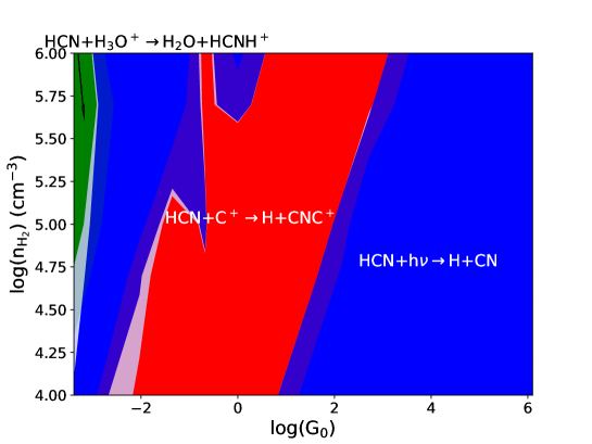
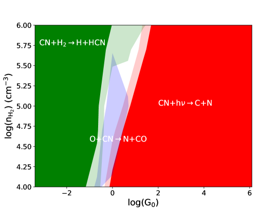
Figure 22: Dominant reactions of HCN (upper panel) and CN (bottom panel) destruction assuming $T\leavevmode\nobreak\ =\leavevmode\nobreak\ 300$ K. Reactions contributed at least 50$\%$ of total flux are marked with full colors. Transparent colors correspond to 30$\%$-50$\%$ contribution. HCN + h$\nu$ $\rightarrow$ H + CN reaction is shown in blue, HCN + C⁺ $\rightarrow$ H + CNC⁺ in red, and HCN + H₃O⁺ $\rightarrow$ H₂O + HCNH⁺ in green. CN + h$\nu$ $\rightarrow$ C + N reaction is marked with red color, O + CN $\rightarrow$ N + CO with blue color and CN + H₂ $\rightarrow$ H + HCN with green color.

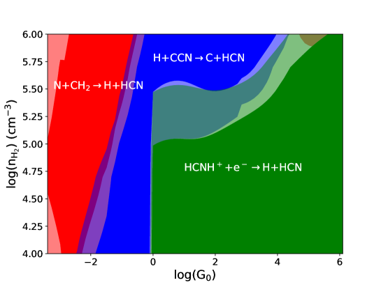
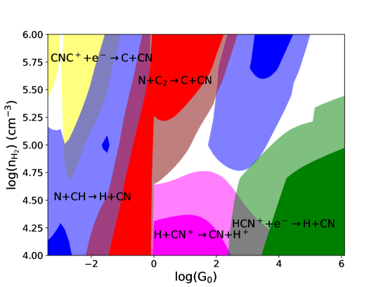
Figure 23: Similar to Figure 22 but for HCN (upper panel) and CN (bottom panel) production assuming $T\leavevmode\nobreak\ =\leavevmode\nobreak\ 50$ K. HCNH⁺ + e^- $\rightarrow$ H + HCN reaction is marked with green color, H + CCN $\rightarrow$ C + HCN with blue color and N + CH₂ $\rightarrow$ H + HCN with red color. HCN⁺ + e^- $\rightarrow$ H + CN reaction is marked with green color, N + C₂ $\rightarrow$ C + CN with red color, CNC⁺ + e^- $\rightarrow$ C + CN with yellow color, N + CH $\rightarrow$ H + CN with blue color and H + CN⁺ $\rightarrow$ CN + H⁺ with magenta.