]{} #1 \delimsize— #2
Effective Scenarios in Multistage Distributionally Robust Optimization with a Focus on Total Variation Distance
Abstract
We study multistage distributionally robust optimization (DRO) to hedge against ambiguity in quantifying the underlying uncertainty of a problem. Recognizing that not all the realizations and scenario paths might have an “effect” on the optimal value, we investigate the question of how to define and identify critical scenarios for nested multistage DRO problems. Our analysis extends the work of Rahimian, Bayraksan, and Homem-de-Mello [Math. Program. 173(1–2): 393–430, 2019], which was in the context of a static/two-stage setting, to the multistage setting. To this end, we define the notions of effectiveness of scenario paths and the conditional effectiveness of realizations along a scenario path for a general class of multistage DRO problems. We then propose easy-to-check conditions to identify the effectiveness of scenario paths in the multistage setting when the distributional ambiguity is modeled via the total variation distance. Numerical results show that these notions provide useful insight on the underlying uncertainty of the problem.
Keywords: Multistage distributionally robust optimization, Effective scenarios, Total variation distance
1 Introduction
Many decision-making problems are dynamic and stochastic, where the realizations of the stochastic process are revealed over time and the decisions are made sequentially with the available information [26]. Such problems have been modeled using multistage stochastic programming [9, 45] and adjustable robust optimization [4], among others. These approaches traditionally assume that the distribution of the stochastic process is known. However, this is rarely true in real life. Motivated by the fact that, in practice, a modeler might have some—albeit imperfect—distributional information about the uncertain parameters, a modeling approach, referred to as distributionally robust, has recently attracted considerable attention [27]. Pioneered by [36], such an approach assumes that the underlying probability distribution is unknown and lies in an ambiguity set of probability distributions. When used in a decision-making framework, the distributionally robust optimization (DRO) approach may protect the decision-maker from the ambiguity in the underlying probability [13, 6].
In this paper, we study a DRO approach to a sequential decision-making problem in the spirit of multistage stochastic programming. We refer to this model as multistage DRO. Most of the papers in this area focus on the computational aspects, proposing decomposition algorithms like specialized nested Benders’ decomposition [e.g., 22] or stochastic dual dynamic programming [e.g., 18, 24, 14, 47], or modeling aspects on how to form the ambiguity sets [e.g., 8, 23]. In this paper, we study multistage DRO from a different point of view. Our aim is to gain insight into the scenarios that can impact the optimal value.
While the literature on static/two-stage DRO models is quite mature by now [e.g., 27, 21, 3], there are relatively few papers on multistage DRO. Some works consider moment-based models [37, 44, 7, 47], and others consider discrepancy-based models: nested Wasserstein distance [23], -Wasserstein [8], distance [20], modified distance [24], norm [18], and general class of -divergences [22]. In [14], the authors allow for the inclusion of moment constraints as well as discrepancy-based constraints, such as Wasserstein and total variation metrics. In [46], the authors study data-driven multistage problems in which the input process can be represented by a Hidden Markov Model (HMM), and apply DRO to account for estimation errors of the HMM transition matrix. The authors in [42] and [25] study general multistage DRO models from the theory of rectangular ambiguity sets and the connection to decomposability and time consistency of the resulting dynamic risk measures.
Modeling distributional ambiguity in a multistage DRO is more complicated than the static/two-stage setting, and it is tied to the time consistency of the policies [e.g., 32, 11, 38]. In order to enforce time consistency of a multistage DRO, we model the ambiguity in a nested way (see Section 2.1). That is, at each stage, we form a conditional ambiguity set, conditioned on the available information so far, to model the ambiguity in the distribution of the next stage’s uncertain parameters. Associated with an optimal policy to such a formulation is a worst-case probability distribution. What does this distribution look like? What information can be gained from it? Such questions are raised in the context of static/two-stage DRO models in [28], and in this paper, we study similar questions for a multistage DRO.
Assuming a stochastic process with a finite number of scenarios, the authors in [28] define the notions of effective and ineffective scenarios for a static/two-stage DRO (reviewed in Section 2.3). Effective scenarios are those that lead to changes in the optimal value if removed from the ambiguity set (more precisely, forced to have a zero probability). Likewise, ineffective scenarios are those that can be removed from the ambiguity set without causing any change to the optimal value. It is shown in [28] that one cannot determine whether a scenario is effective or not simply by looking at the worst-case probabilities. Indeed, it is possible to have an effective scenario with a zero worst-case probability and an ineffective scenario with a positive worst-case probability. Such a phenomenon is later tied to the existence of a strict monotone risk measure in [42], a concept related to the time consistency of risk-averse multistage models. In [28], the authors provide easy-to-check conditions to identify effective/ineffective scenarios when the distributional ambiguity is modeled via the total variation distance around a nominal distribution, and in [29], these are generalized to static/two-stage DRO with continuous distributions in the context of inventory problems. These easy-to-check conditions provide computational and practical advantages over the naïve resolving of the corresponding problems multiple times (once they are forced to have a zero probability in the ambiguity set) and observing the cases in which there were any changes to the optimal value. In [2], the idea of effective scenarios is applied to risk-averse optimization problems, thereby yielding a scenario reduction method for such problems.
The notion of effective scenarios resonates with related concepts proposed in the literature, some of them quite recently. One such concept is that of a coreset [1]: given a set of points , a coreset is “an easily computable subset , so that solving the underlying problem on gives an approximate solution to the original problem,” an idea that has found applications particularly in some statistical learning methods such as clustering, k-medians, and regression, among others. Another related concept is that of supporting constraints [10], defined for a class of problems in which each constraint corresponds to a scenario. In that context, a constraint is said to be supporting if its removal changes the optimal solution of the problem. The authors use this notion to estimate the probability that, given a problem with constraints, a new randomly selected th constraint is violated by the optimal solution of that problem. The idea of effective scenarios can also be viewed from the perspective of problem-driven scenario reduction, where the goal is to find what are the “essential” scenarios that must be kept from an original set of scenarios so that solving the problem over the reduced set yields the same optimal solution (or optimal value) as the original one; see [15] for the development of such ideas in the context of risk-averse optimization problems, leading to the notion of risk regions which turn out to be very much related to the results in [2]. In [5], a new distance between two distributions that considers the objective function values is defined for problem-driven scenario reduction in two-stage problems. All these concepts notwithstanding, to the best of our knowledge, no concept related to the notion of effective scenarios has been proposed in the context of multistage problems.
In this paper, we generalize the notion of effective/ineffective scenarios to a multistage DRO. As one might anticipate, these notions are nontrivial and more subtle in a multistage setting and several questions arise, even under a finite stochastic process:
-
1.
Should we study them for the entire realizations of the stochastic process—a scenario path—for a finite stochastic process represented by a scenario tree?
-
2.
Should we study them for the realizations along a scenario path, at each stage separately?
-
3.
Is there any connection between the effectiveness of a scenario path and the effectiveness of realizations along the path?
In this paper, in agreement with our desire to have a time-consistent multistage DRO model, we limit ourselves to a nested formulation and provide rigorous mathematical definitions for both the effectiveness of a scenario path and the effectiveness of separate realizations along a path. The effectiveness of a scenario path is defined with respect to a change in the optimal value once that scenario path is removed (Section 3.1). On the other hand, the effectiveness of a realization along a scenario path is defined conditionally, given the available information (Section 3.2). Henceforth, we refer to them as conditionally effective/ineffective realizations. To provide an answer to the third question above, we focus on a multistage DRO, where the conditional distributional ambiguity is modeled via the total variation distance (referred to as a multistage DRO-V). In this setting, we provide an affirmative answer; yes.
By exploiting the structure of the conditional ambiguity sets formed via the total variation distance, we show that the easy-to-check conditions proposed in [28] are applicable to identify the conditional effectiveness of realizations along a scenario path. We then show that a scenario path is effective if and only if all realizations along the path are conditionally effective (Theorem 1). This result is interesting—and somewhat surprising—because it says that checking effectiveness in a one-step-ahead fashion suffices to determine the effectiveness of the entire path.
Besides providing a rigorous answer to the third question above, which yields both a practical/computational advantage and a conceptual/managerial perspective in identifying effectiveness of scenario paths, our choice to work with the total variation distance has other benefits. The first one is risk interpretation: As we shall see in Section 4.1, when the total variation distance is used to define the conditional ambiguity sets, the resulting multistage DRO is equivalent to minimizing a composite coherent risk measure, consists of nested coherent risk measures. The second benefit is computational: The problem reduces to a computationally tractable optimization model and is amenable to a numerical decomposition algorithm. This is of particular importance in a multistage setting as the stochastic process is typically discretized and hence, it gives a computational advantage over other metrics such as a general Wasserstein distance. Finally, the total variation distance resides in the intersection of three classes of discrepancy measures commonly used in DRO: It is a metric, a -divergence, and a special case of the Wasserstein distance when the distance between two scenarios is (when the scenarios are the same) or (when they are different).
To summarize, the contributions of this paper are as follows. We introduce, to the best of our knowledge for the first time, the notions of effectiveness for realizations and scenario paths for a general class of nested multistage DRO under a finite stochastic process. We provide easy-to-check conditions to identify the conditional effectiveness of realizations for multistage DRO-V. Our main result ties the effectiveness of a scenario path to the conditional effectiveness of realizations along the path. We numerically illustrate how the concepts introduced and the main results of the paper provide managerial insight to the underlying uncertainty of a multistage DRO.
The rest of this paper is outlined as follows. In Section 2, we define the class of multistage DRO problems we are interested in, establish notation, and review background information on effective scenarios for a static DRO. In Section 3, we define the notions of effectiveness of scenario paths and conditional effectiveness of realizations for a multistage DRO. In Section 4, we define a multistage DRO-V and present its risk interpretation. Section 5 provides easy-to-check conditions to identify the conditional effectiveness of realizations and the effectiveness of scenario paths for a multistage DRO-V. We then present numerical experiments and provide managerial insights in Section 6. Finally, we end with conclusions in Section 7.
2 Background and Notation
2.1 Multistage DRO
We study a class of multistage stochastic optimization problems with stages. To formally define the class of problems we are interested in, consider a measurable space . The uncertain parameters are gradually realized over time and are represented by a stochastic process on the probability space, where and is composed of the random parameters in stage . We assume that , , has finitely many possible realizations, where is a degenerate random vector (i.e., constant). Let denote the history of the stochastic process up to (and including) time . The filtration associated with is defined by , where is the -algebra generated by , and .
As information on the stochastic process becomes available at stage , a decision must be made based on the available information so far. These decisions define a decision rule or policy . A basic requirement of multistage stochastic optimization problems is the unimplementablity and nonanticipativity of policies [45, Chapter 3]. That is, decision , , must depend only on the information available up to time and must not depend on neither the future realizations of the stochastic process nor the future decisions. Similar to , we use to denote a policy up to (and including) time , i.e., .
Consider a multistage DRO problem of the form
| (T-DRO) |
In stage , , the set-valued mapping denotes a non-empty, compact polyhedral feasibility set, and is a random, real-valued polyhedral function, with the decision and the realized uncertainty given111To simplify the exposition and focus on the concepts rather than technicalities, throughout we assume that is a polyhedral set and is a random polyhedral function, . Nevertheless, the results in this paper can be extended to general convex sets and functions under appropriate constraint qualification conditions.. For nonanticipativity, we force to be -measurable, , by assuming both and are -measurable. Moreover, is the conditional ambiguity set for the conditional distribution of , conditioned on , . The set contains all conditional probability distributions induced by , given . Also, denotes the conditional expectation with respect to .
The inner maximization problems in (T-DRO) hedge against the worst-case probability distribution in the conditional ambiguity set , . Associated with an optimal policy to (T-DRO) is an optimal worst-case probability distribution . An optimal probability distribution , or in general, a (push-forward) probability distribution induced by on , should be understood in similar sense to a policy. That is, at each stage , , given the available information on , the conditional probability of can be determined.
While there are various ways to model the conditional distributional ambiguity in (T-DRO), we do not assume any particular structure on until Section 4. Note that when contains only the nominal conditional distribution of , conditioned on , (T-DRO) reduces to the classical multistage stochastic program. Hence, by the monotonicity and the translation invariance of the expectation, this formulation can be written in a nonnested form.
Remark 1.
It is tempting to form a multistage DRO problem of the form
| (1) |
where the ambiguity set is a subset of all probability measures on . While such a formulation is valid, it is not automatically time consistent. In the sense of the sequential optimality conditions of a policy [38, 32, 40], time consistency implies that “decisions made today should agree with the planning made yesterday for the scenario that actually occurred” [17]. In fact, (1) is time consistent if and only if the risk measure corresponding to the inner maximization problem in (1) is decomposable into a (nested) sequence of conditional risk mappings and satisfies a strict monotonocity property [39, 42, 43]. The decomposability property lends itself to a rectangular set associated with set . We refer interested readers to [41] for topics on the existence and construction of a rectangular set.
It is known the time-consistent formulation (T-DRO) naturally leads to the so-called Bellman’s principle of optimality to derive dynamic programming (DP) equations. These equations play an important role in the analysis of the effectiveness of the scenario paths and the conditional effectiveness of realizations along a scenario path in this paper. We now present these equations for future references.
Consider (T-DRO) at a given stage , , when all information from the previous stages, given by and , is known. Throughout the paper, we use the vacuous notation for convenience. Going backward in time, we can derive DP reformulation of (T-DRO), where the cost-to-go (value) function at stage , , is as follows
| (2) |
We refer to as the worst-case expected problem at stage . We assume that is finite and integrable for any distribution in , . By convention, we set the worst-case expected problem at stage to zero. Moreover, we denote the optimal value simply with .
Remark 2.
Throughout this paper we assume that an optimal policy satisfies the DP equations, possibly obtained via a nested Benders’ decomposition algorithm [9]. An optimal policy that satisfies the DP equations is time consistent because for every stage , , is an optimal solution to problem (2) for every realization of the random vector .
2.2 Scenario Tree Notation
Recall that we assume the stochastic process in stages is represented by , where . We denote the support of by , . We let . Because we assume a finite sample space, a scenario tree with stages represents all the possible ways that the stochastic process evolves.
We associate each realization of the random vector to a node in stage of the scenario tree, . We denote the set of nodes at stage by , and denotes an element in that set. By assumption, is a singleton, containing the root node . We use the notation () to indicate a specific realization of the random vector () at node . Because of the one-to-one correspondence between and , we may use them interchangeably, both in words and notation. For example, we may use as a shorthand notation for . In particular, there is a one-to-one correspondence between at the last stage and a realization . We use to refer to a generic node in stage of the tree as well as a realization of the stochastic process. By construction, a realization is determined by a path from the root node to a leaf node . Such a generic path is uniquely identified with , and we refer to as a scenario path throughout the paper.
A node (), has a unique immediate ancestor in stage , denoted by , and a node has a set of immediate children in stage , denoted by . By definition, and . For a subset , , we also define to denote the set of all nodes that have at least one child in . For , we define a projection mapping which returns the stage- node that the scenario path is going through. By definition, we have and for all . For , we use to denote the nominal conditional probability of given , i.e., , We may use as a shorthand notation for the ambiguity set . We also use , , in a similar manner as the nominal conditional distribution . We use boldface letter to denote a probability vector.
2.3 Background on Effective Scenarios for a Two-Stage DRO
Consider a special case of (T-DRO) with . To minimize notational overload, let us drop stage indices. Let denote the set of scenarios, with as a generic element in . Given this setup, a two-stage DRO problem can be written as
| (2-DRO) |
where is defined as in (2) for a fixed and , and is an ambiguity set of probability distributions. Let us consider a subset of scenarios . The idea behind identifying the effectiveness of scenarios in is to check whether the optimal value of (2-DRO) changes once these scenarios are “removed” from the ambiguity set, or more precisely, they are forced to have a zero probability. To that end, the authors in [28] define the so-called assessment problem of scenarios in as follows
| (3) |
where is the ambiguity set of distributions for the assessment problem of scenarios in . Observe that we have
| (4) |
where is an optimal solution to (2-DRO).
Definition 1.
[28, Definition 1] A subset is called effective if . A subset is called ineffective if it is not effective.
Remark 3.
A sufficient condition for a subset of scenarios to be effective is . If the assessment problem (3) is not well defined (i.e., is infeasible), the corresponding subset of scenarios is effective by definition. ∎
3 Effective Scenarios for a Multistage DRO
In this section, we extend the notion of effective scenarios, introduced in [28] for a static DRO, to (T-DRO). We address the effectiveness of scenarios for (T-DRO) in two ways: effectiveness of scenario paths (Section 3.1) and conditional effectiveness of realizations (Section 3.2).
3.1 Effective Scenario Paths for a Multistage DRO
The idea behind identifying the effectiveness of scenario paths is to verify whether the optimal value of (T-DRO) changes when a scenario path (or, more generally, a set of scenario paths) is removed from the problem. As in [28], the first task is then to define what is meant by “removing” a set of scenario paths from the problem. We remove scenario paths in by forcing the probability of these scenario paths to be zero. By the construction of a scenario tree, the probability of a scenario path is calculated by the product of conditional probabilities, associated with the nodes along the path. Thus, forcing the probability of a scenario path to zero can be achieved by setting the conditional probability of the corresponding leaf node to zero. It is worth noting that setting the conditional probability of any other node along the path, besides the leaf node, to zero forces the probability of all scenario paths that are going through that node, to zero, which is undesirable. Moreover, because the ambiguity sets in (T-DRO) are defined conditionally, we need to set the conditional probability of the corresponding leaf node to zero in an appropriate conditional ambiguity set, more precisely, in .
3.1.1 Assessment Problem of Scenario Paths
To identify the effectiveness of scenario paths in we define an appropriate assessment problem. In order to elaborate on the notion of removal of scenario paths and the assessment problem in the multistage setting, let us define more notation. Recall the definition of , the set of all nodes that have at least one child in . For each , let us define for the set of its children in . Thus, .
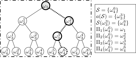
For any , we remove the scenario paths in by restricting the ambiguity set to those probabilities for which ; see Figure 1 for an illustration. This ensures that the scenario paths in are not in the support of any worst-case probability distribution induced by . We shall call the problem that removes all scenario paths in the assessment problem of scenario paths in . More formally, this problem can be formulated as
| (5) |
where for , the last-stage conditional ambiguity set of distributions for the assessment of the scenario paths in is defined as . For , we set . Notice that (5) is similar to problem (T-DRO), except for the last stage where is replaced with , with the interpretation mentioned above. Moreover, notice that the assessment problem (5) does not eliminate scenario paths from the sample space; it only enforces , , for all . Also, when , (5) reduces to (T-DRO).
3.1.2 DP Reformulation of the Assessment Problem
In order to mathematically define the notion of effectiveness of scenario paths for (T-DRO), we need to establish the relationship between the optimal values of the original problem (T-DRO) and the assessment problem (5) precisely. To do this, we first write the DP reformulation of (5) in a similar manner to those of (T-DRO).
Consider the assessment problem (5) at a given stage , , when all information from previous stages (given by and ) is known. Let denote the optimal value to this problem. Because there is no inner maximization problem at stage (i.e., ; see Section 2.1), we set
| (6) |
For , on the other hand, we have
| (7) |
Going backward in time, one can obtain for , as
| (8) |
Equations (6)–(8) present the DP reformulation of (5). Note that the maximization in (7) is done over , whereas it is done over in (8). For brevity, we denote the optimal value of (5) as . Throughout the paper, we use notation to differentiate the cost-to-go functions for the assessment problem of the scenario paths in , presented in this section, from the cost-to-go functions of the original problem (T-DRO), presented in Section 2.1.
3.1.3 Definition and Properties
In this section, we precisely define the effectiveness of scenario paths for (T-DRO) and state some relevant properties.
Proposition 1.
Consider two sets . Then, .
Proof.
Let denote an optimal policy obtained by solving the DP reformulation of (5) for . For any and , the corresponding worst-case expected value problem at stage in (5) for is more restricted than the corresponding problem in (5) for . This, combined with the suboptimality of to problem (5) for , implies that
where we also used the fact that . The equality above is due to the time consistency of (recall Remark 1). Going backward in time for , we have
where the second inequality is due to and the equality is due to the time consistency of . Consequently, we have
where the first inequality is due to the suboptimality of to problem (5). ∎
By taking and in the proof of Proposition 1, we have
| (10) |
where is the optimal value of (T-DRO) and is an optimal policy to (T-DRO). With this relationship, we can now define effective scenario paths.
Definition 2 (Effectiveness of scenario paths).
A subset of scenario paths is called effective if . A subset of scenario paths is called ineffective if it is not effective.
In words, a subset of scenario paths is called effective if the optimal value of the corresponding assessment problem (5) is strictly smaller than the optimal value of (T-DRO). Similar to Remark 3 for (2-DRO), a sufficient condition for a subset of scenario paths to be effective is . Moreover, the assessment problem of scenario paths in might not be well defined. For instance, if for some , too many scenario paths are restricted to have a zero worst-case probability (e.g., ), then, the inner maximization problem at stage might become infeasible. In this case, we set the optimal value of (5) to by convention and is effective by definition.
One can conjecture that the effectiveness of a subset of scenario paths might be affected in interaction with other subsets of scenario paths. The following proposition addresses the effectiveness of union of an effective subset of scenario paths and intersection of an ineffective subset of scenario paths with any other subset of .
Proposition 2.
(i) The union of an effective subset of scenario paths with any other subset of is effective. (ii) The intersection of an ineffective subset of scenario paths with any other subset of is ineffective.
Proof.
Corollary 1.
A subset of an ineffective subset of scenario paths is ineffective.
It is worth noting that Definition 2 for (T-DRO) is not an immediate extension of Definition 1 for (2-DRO), and there are subtle but important differences. To explain this, let us focus on (10) and (4), the relationships that form the bases for establishing these definitions. In particular, let us examine the terms in (10) and in (4) in more detail. On the one hand, the ambiguity set is not impacted by the removed subset of scenario paths , whereas is a restricted set and impacted by . On the other hand, the cost-to-go function is impacted by the removed subset of scenario paths , whereas is not. So, (10) does not follow from (4). These differences are themselves due to the differences of the assessment problems (3) and (5). By a similar reasoning, there are subtle, important differences in Proposition 2 and [28, Proposition 2].
3.2 Conditionally Effective Realizations for a Multistage DRO
In this section, we define conditional effectiveness of realizations along a scenario path, given the available information on the history of the stochastic process and decisions. We explain that this notion, unlike the effectiveness of scenario paths, resembles the effectiveness of scenarios for (2-DRO).
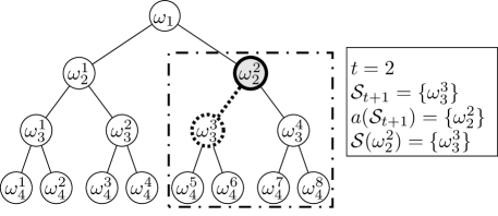
To identify conditionally effective realizations, as it might be perceived from the name, first, one has to consider all information from previous stages, and then, evaluate what would happen to the optimal cost going forward if a subset of realizations is conditionally removed. Suppose that and , , are given. The idea behind identifying conditionally effective realizations is to verify whether the cost-to-go function (2) at stage changes when a realization (or, more generally, a set of realizations) in stage is conditionally removed from the problem. We “conditionally remove” realizations by forcing the conditional probability of these realizations to be zero, conditioned on the history of the stochastic process.
Note that because the ambiguity sets in (T-DRO) are defined conditionally, we need to set the conditional probability of to zero in an appropriate conditional ambiguity set, more precisely, in . Moreover, because is forced to have a zero conditional probability, all scenario paths that are going through will have a zero conditional probability, conditioned on . Hence, all such scenario paths will have a zero probability. This implies that the way the removal of scenario paths is defined in Section 3.1 is different from how we define the conditional removal of realizations in this section. Furthermore, once scenario paths are removed in Section 3.1, we compare the optimal objective function values at the root node . Here, we look for changes in the cost-to-go value functions . In this section, we follow a similar process to what did in Section 3.1; nevertheless, the developments have different interpretations.
3.2.1 Conditional Assessment Problem for Realizations
Suppose that the history of the stochastic process up to and including stage , , is given. Recall that is the set of realizations to be conditionally removed. For each , let us define to denote the set of all children of in . Thus, . For any , we conditionally remove the realizations in by restricting the ambiguity set to those probabilities for which (see Figure 2 for an illustration). This ensures that all scenario paths that are going through any node in as part of their process are not in the support of any worst-case probability distribution induced by . Conditioned on and , we define the conditional assessment problem of realizations in as
| (11) |
where for , the conditional ambiguity set of distributions for the conditional assessment problem of realizations in is defined as . For , . Notice that problem (11) is similar to problem (2), except for in stage where is replaced with , with the interpretation mentioned above. Moreover, notice that the assessment problem (11) does not eliminate the realizations from the sample space ; it only enforces , , for . As before, when , (11) reduces to (2).
3.2.2 DP Reformulation of the Assessment Problem
To mathematically define conditionally effective realizations for (T-DRO), we need to establish the relationship between the optimal values of (2) and (11). As in for the effectiveness of scenario paths in Section 3.1.2, we first need to derive the DP reformulation of (11).
Consider the optimization problem (11) at a given stage , , when all information from previous stages (given by and ) is known. By the construction of (11), forcing the conditional probability of a realization at stage to zero does not affect the way the cost-to-go functions at stage , for , are written. Thus, we have
| (12) |
where , , are defined as in (2). For brevity, we denote the optimal value of the conditional assessment problem of the realizations , in stage , with . Throughout the paper, we use notation to differentiate the cost-to-go function at stage for the conditional assessment problem of the realizations in , presented in this section, from the cost-to-go function of the original problem (T-DRO), presented in Section 2.1.
3.2.3 Definition and Properties
We now formally define the notion of the conditional effectiveness of realizations for (T-DRO) and discuss its properties.
Proposition 3.
Consider a fixed , a subset of realizations , a partial optimal policy to (T-DRO) up to stage , and . Then, .
Proof.
Definition 3 (Conditional effectiveness of realizations).
Consider a fixed , a subset of realizations , partial optimal policy to (T-DRO), and . A subset of realizations is called conditionally effective if . A subset of realizations is called conditionally ineffective if it is not conditionally effective.
We conclude this section with a comment on the similarity between Definitions 1 and 3. Observe that (2) resembles the structure of (2-DRO). Similarly, (12) resembles the structure of (3). Consequently, the relationship between (2-DRO) and (3), as stated in (4), can similarly be made about (2) and (12). That is, given and , by the proof of Proposition 3, we have
| (13) |
Observe that the relationships in (13) are similar to those of (4). This similarity is not by surprise. In fact, the conditional assessment problem (11) is defined in a similar manner to (3). Hence, Definitions 1 and 3 are similar. Consequently, the results in [28] on the effective scenarios for (2-DRO) will hold for the conditional effectiveness of realizations in (T-DRO). This is not true for the effectiveness of scenario paths, defined in Section 3.1. We shall shortly exploit this similarity in Section 5 to identify the effectiveness of scenario paths by connecting it to the conditional effectiveness of realizations along a path for (T-DRO) formed via the total variation distance.
4 Multistage DRO with the Total Variation Distance
We now narrow down our focus to the multistage DRO formed via the total variation distance. This model, referred to as T-DRO-V for short, is formulated in the same manner as (T-DRO), with the conditional ambiguity sets as follows:
| (14) |
where is the total variation distance between two (conditional) distributions and . The conditional ambiguity set , , contains all conditional probability distributions whose total variation distances to the nominal conditional distribution are limited above by the level of robustness . Note that is bounded above by one and bounded below by zero. Hence, without loss of generality, we assume . Also, the levels of robustness at each stage , , may depend on , and , , may depend on . We drop these dependencies for ease of exposition. We can then obtain the cost-to-go function as in (2), where the worst-case expected problem is calculated via in (14).
4.1 Risk-Averse Interpretation
It is known that under suitable assumptions, a DRO model pertains to a risk-averse optimization model. As it is shown in [28] such a risk-averse interpretation plays an important role in identifying effective scenarios for a static DRO. Not surprisingly, we shall shortly see that the risk-averse interpretation of T-DRO-V plays an important role in identifying the effectiveness of scenario paths and the conditional effectiveness of realization as well.
The conditional ambiguity set , , defined in (14), is a convex compact subset of , the set of all discrete probability distributions induced by , given . Moreover, is integrable on by the assumptions stated in Section 2.1. Recall the dual representation of a coherent risk measure; see, e.g., [45, Theorem 6.7], [39, Theorem 3.1], [34, Theorem 2.2]. By a similar procedure applied to conditional distributions, as done for example in [23], one can show that the worst-case expected problem is equivalent to a real-valued conditional coherent risk mapping [35, 34, 39]. By induction and going backward in time, we can show that T-DRO-V is equivalent to a risk-averse stochastic optimization problem involving nested coherent risk measures.
Proposition 4.
T-DRO-V is equivalent to
| (15) |
where , , is the conditional coherent risk measure given by
Proof.
In Proposition 4, is taken conditionally with respect to the support set and is the conditional value-at-risk (CVaR)222Here, denotes the CVaR of at the confidence level , , defined as , where is the value-at-risk (VaR) at level [30]. taken with respect to the nominal conditional distribution at level . Per usual convention, we set and , . Hence, when for , T-DRO-V reduces to the risk-neutral model. As increases, more weight is put on the worst-case cost, and T-DRO-V becomes more conservative. When , T-DRO-V reduces to minimizing the worst-case total cost over the support of .
5 Identifying Effectiveness of Scenario Paths and Realizations for a Multistage DRO-V
For a general multistage DRO with a finite sample space, we introduced the notions of the effectiveness of scenario paths and the conditional effectiveness of realizations in Sections 3.1 and 3.2, respectively. In this section, we focus on T-DRO-V and present easy-to-check conditions to identify the effectiveness of scenario paths/realizations.
Let us first focus on the conditional effectiveness of realizations along a scenario path. As discussed at the end of Section 3.2, by construction, effective scenarios for (2-DRO), as stated in Definition 1, are defined similarly to the conditionally effective realizations for (T-DRO), as stated in Definition 3. In particular, one can make the following observation for T-DRO-V.
Observation 1.
In other words, given the history of decisions and stochastic process, one can easily identity conditionally effective and ineffective realizations for T-DRO-V by using the easy-to-check conditions proposed in [28, Theorems 1–3] for (2-DRO) via the total variation distance. We briefly mention the general ideas of these results next.
5.1 Background on Identifying Effective Scenarios for a Two-Stage DRO-V
When the distributional ambiguity is modeled via the total variation distance, (2-DRO) can be written as
| (2-DRO-V) |
where and denotes the total variation distance between two probability distributions and . Assume that . Before we discuss the general structure of results in [28], let us define some notation. For a fixed , let . For any , we use as shorthand notation for the set . With some abuse of notation, let . For a fixed , we use to denote . Given , let be the left-side -quantile of distribution of or equivalently, the VaR of at level : [31].
Motivated by the risk-averse interpretation of (2-DRO-V) (see Proposition 4 with ), the authors in [28] define the following sets, collectively referred to as primal categories, that partition the scenario set : , , , and . Let solve (2-DRO-V). For a moment, suppose that the nominal probabilities are all positive, i.e., for all . Then, according to [28], all scenarios in are effective, while scenarios in are ineffective. For scenarios in , the situation is more delicate. For example, if , all scenarios in are ineffective. Otherwise, if and there is only one scenario in , that scenario must be effective. Note that easy-to-check conditions may not identify the effectiveness of all scenarios in . We refer the readers to [28, Theorems 1–3] for detailed results.
5.2 Main Result for a Multistage DRO-V
Recall that according to Theorem 1 one can identify the conditional effectiveness of realizations using the easy-to-check conditions stated in [28, Theorems 1–3]. We refer to the realizations whose conditional effectiveness is identified by these results as identifiably conditionally effective or ineffective. We now present our main result, connecting the effectiveness of scenario paths to the conditional effectiveness of realizations along the path.
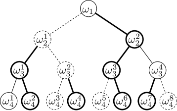
Theorem 1.
A scenario path is effective for T-DRO-V if and only if is identifiably conditionally effective for T-DRO-V for all , .
As a result of Theorem 1, in order to identify the effectiveness of a scenario path for T-DRO-V, we need to first identify the conditional effectiveness of all realizations along the path using the easy-to-check conditions stated in [28, Theorems 1–3]. If all realizations along the path are identifiably conditionally effective, then the scenario path is effective for T-DRO-V. Otherwise, if there is at least one realization along the path that is identifiably conditionally ineffective, then the scenario path is ineffective for T-DRO-V. As in [28], we might not be able to identify the effectiveness of all scenario paths for T-DRO-V because the easy-to-check conditions might not be able to do so for the conditional effectiveness of realizations. Figure 3 illustrates the usage of Theorem 1 to identify the effectiveness of scenario paths for T-DRO-V.
We now turn our attention to the proof of Theorem 1. Before presenting the proof, we state two technical lemmas. Lemma 1 makes a connection between the maximizers of a worst-case expected problem and an identifiably conditionally effective/ineffective realization. Lemma 2 states optimality conditions for the assessment problem of scenario paths in for T-DRO-V.
Lemma 1.
Let be an optimal policy to T-DRO-V. Consider a realization at stage , where . Given and , let denote the set of optimal (conditional) probability distributions to the worst-case expected problem at stage , i.e.,
| (16) |
where is defined as in (14). The following statements hold for .
-
(i)
If is identifiably conditionally effective for T-DRO-V, then, for any , we have . Moreover, .
-
(ii)
If is identifiably conditionally ineffective for the T-DRO-V, then, for any , we have . Moreover, .
Proof.
The proof of the first parts in (i) and (ii) follows from [28, Theorems 1–3], combined with [28, Proposition 4]. To prove the second part of (i), first note that we have the equality as argued in the proof of Proposition 3 and by the time consistency of . The inequality then follows from the fact that and the finiteness of the sample space . The second part of (ii) is immediate from Definition 3. ∎
Lemma 2.
Consider a feasible policy to T-DRO-V. Let denote the normal cone of at , , defined as . Moreover, let
| (17) |
. The policy is optimal to the assessment problem of scenario paths in corresponding to T-DRO-V if and only if
-
(i)
holds true for every ,
-
(ii)
holds true for every , and
-
(iii)
holds true for every and ,
where denotes the convex hull.
Proof.
Let us consider the DP reformulation (6)–(8) of the assessment problem of scenario paths in corresponding to T-DRO-V, similar to those in Section 3.1.2, where the conditional ambiguity sets are formed as in (14). Similar to the proof of [45, Proposition 3.4], using [33, Theorem 51] and Moreau-Rockafellar theorem [45, Theorem 7.4], we can write the optimality conditions at stage as . At , the optimality conditions can be stated as holds true for every . Now, using [16, Corollary 4.3.2] yields the optimality conditions at . The proof for follows similarly. ∎
Note that when , Lemma 2 gives the optimality conditions for T-DRO-V.
Proof of Theorem 1.
Let , for , i.e., the scenario path is given with the sequence , where . Moreover, let be an optimal policy to T-DRO-V and denote an optimal worst-case probability distribution corresponding to . We first prove that if is identifiably conditionally effective for all , then is effective. Then, we prove that if there exists , , such that is identifiably conditionally ineffective, then is ineffective. In the proof, we frequently use the time consistency of for T-DRO-V, as well as the DP reformulations discussed in Sections 2.1, 3.1.2, and 3.2.2, all tailored for the conditional ambiguity sets of the form (14).
“:” To prove the result, we need to show that . By the hypothesis and using Definition 3, we have , . Using Lemma 1(i), we have
| (18) |
which for all implies
| (19) |
Let us look into the values of and on the whole scenario tree. Recall by Remark 4 that the only realization whose cost-to-go function at stage is affected by the removal of the scenario path is , . That is, for a feasible policy to T-DRO-V, (9) simplifies to
| (20) |
Now, we look into and along the scenario path . Starting at stage , we have
| (21) |
where the first inequality is due to the suboptimality of to the assessment problem of the scenario path , the first equality is due to the fact and are the same given , the second inequality is due to (18), and the second equality is due to the time consistency of . Thus, for any with , i.e., , we have
| (22) |
where the first equality is due to (20), (21), and the finiteness of . The inequality comes from (19) and the second equality is due to the time consistency of . On the other hand, for any with , i.e., , we have
| (23) |
where the first inequality comes from (20), (21), and the finiteness of . Now, note that can be written as the union
Thus, putting the inequalities (22) and (23) together, we conclude
| (24) |
where the first inequality is due to the suboptimality of to the assessment problem of the scenario path . We can reach a similar conclusion in stage , where we use (24) instead of (21) and use (20) for . Continuing this process backward in time, we conclude , implying the scenario path is effective for T-DRO-V using Definition 2.
“:” To prove the result, we construct a policy , defined below, and we show that such a policy is optimal to the assessment problem of the scenario path , corresponding to T-DRO-V. Then, by Definition 2, to prove that the scenario path is ineffective, it suffices to show that for the policy , we have . Note that associated with is an optimal probability .
For the scenario path , suppose that denotes the largest stage, where there is an identifiably conditionally ineffective realization. That is, is either conditionally unidentified or effective, , while is identifiably conditionally ineffective. We construct a policy as , where is a (partial) policy obtained from solving the assessment problem in stage , given and , with the ambiguity sets formed as in (14).
We start the proof by showing that the policy , constructed as above, is optimal for the assessment problem of the scenario path . In order to do this, we first claim that for all (defined as in (16) for and ) and (defined as in (17) for , , and ). Then, we use the optimality conditions stated in Lemma 2 for the assessment problem. To prove the above claim, first observe that
| (25) |
where the equality is due to by construction, and the inequality follows a similar argument as in the proof of Proposition 1. Moreover, observe that if , then using (20) at and for the feasible policy , we have . Hence, considering that by construction, for , we have
| (26) |
If , and hence, , combined with (26), we conclude that for and for all and .
Now, suppose that . To prove the claim, we first investigate which of the four primal categories (recall the definition of primal categories in Section 5.1 and in the context of (2-DRO-V)) a realization can belong to at . Observe that considering that and because we assume that , the primal category of at will be either the same as that at or lower (in index) than that at . For ease of exposition, we adopt the following notation:
Now, let us form and , , as described in Section 5.1. Using the above notation, (26) is stated as , . Also, by the hypothesis, we have . Because is identifiably conditionally ineffective, then by Lemma 1(ii), we have . Moreover, by [28, Theorems 1], we have . Thus, . This implies and . Let us consider the following cases:
-
1
: Thus, and . Consequently, the formation of primal categories is the same at and , and we have , .
-
2
and : Because , we have . On the other hand, by [28, Proposition 4]. Thus, although the primal category of might change, we can conclude , , because the primal category of all other scenarios does not change.
-
3
and : If there is no other scenario in with a positive nominal probability, then, . Because , we have by [28, Proposition 4]. On the other hand, we must have for all because . Thus, although scenarios move from to , by [28, Proposition 4], we must have for because . Moreover, because , we must have , by [28, Proposition 4]. Thus, although scenarios move from to , there is no change in their worst-case probabilities. All the other scenarios keep the same primal category as that at . Consequently, , . Now, if there exists another scenario in with a positive nominal probability, then . Thus, all scenarios, except for that moves to , keep their primal categories as that at . Nevertheless, we have , .
In all the above cases, we concluded , . Now, let us bring back our general notation. The above is equivalent to , for all and ; thus, the claim is proved.
To prove the optimality of to the assessment problem we use Lemma 2. Recall that is a (partial) policy obtained from solving the assessment problem in stage , given and , with the conditional ambiguity sets formed as in (14). Thus, optimality conditions stated in Lemma 2 hold for by construction. Now, let us focus on stage . Recall by Remark 4 that the only realization whose cost-to-go function at stage is affected by the removal of the scenario path is . Thus, it remains to verify the optimality conditions for realization . Consider the optimality conditions Observe that the right-hand sides of the optimality conditions above are the same because of the following reasons: (i) by construction, (ii) by (20), and are the exact same functions, for ; hence, they have the same subdifferentials, and (iii) ; in particular, using Lemma 1(ii) we have for any and for any . Consequently, although the subdifferentials of and might be different, they do not contribute to the right-hand sides of the optimality conditions above. Hence, because satisfies the optimality condition for T-DRO-V at stage , then satisfies the optimality condition for the respective assessment problem at stage . Moreover, it can be seen that . Therefore, this fact and the implication from Remark 4 guarantee that because satisfies the optimality condition for T-DRO-V at stage , then satisfies the optimality condition for the respective assessment problem at stage . By induction, we conclude that is optimal to the assessment problem of the scenario path corresponding to T-DRO-V.
Additionally, observe that with a similar reasoning we have , i.e., the policy incurs an objective function value for the assessment problem of corresponding to T-DRO-V that is equal to the optimal value of T-DRO-V, incurred by the policy . Consequently, by Definition 2, we conclude that the scenario path is ineffective. The case that , i.e., is conditionally ineffective, can be argued similarly, although the notation slightly simplifies. This completes the proof. ∎
6 Numerical Illustration
6.1 Experimental Setup
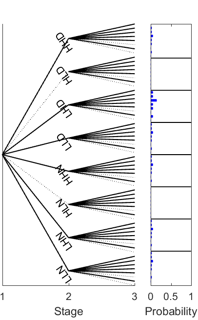
To conduct numerical analyses, we used a version of the water allocation problem described in [48], where now water treatment facilities are subject to disruptions. This problem addresses the allocation of Colorado River water among different users, while meeting uncertain water demand and not exceeding uncertain water supply. The problem originally has 4 stages with the planning period 2010–2050, where both supply and demand uncertainties appear in the right-hand side of constraints. To examine more complex uncertainties besides only the right-hand-side of the constraints and for visual illustration of managerial insights, we generated a smaller three-stage variant of this problem with a 26-year planning horizon as follows. We considered low (L) and high (H) realizations for both the supply and demand uncertainties. In addition, we introduced a random variable to specify whether one of the wastewater treatment plants is disrupted (D) or nondisrupted (N). This leads to randomness in the recourse matrix and can be interpreted as disruption due to natural or man-made disasters. The treatment plant treats wastewater and pumps it back into the system to meet nonpotable (i.e., nondrinkable) water demands like irrigation of parks. This variant has 8 realizations per node ( scenario paths), and we denote it by WATERS3N8. For reference, the labels in the second stage of Figure 4, given as a triplet of (supply, demand, treatment facility), illustrate the second-stage realizations. This pattern repeats in the third stage as well. With respect to the nominal distribution, the stochastic process is interstage independent and all realizations are equally likely for simplicity. We tested interstage dependent cases as well, and the results were similar. We modeled the distributional ambiguity via the total variation distance and assumed that the levels of robustness for all stages are the same (i.e., for all , ). To run the experiments, we varied between 0 and 1 in increments of . We implemented a nested Benders’ decomposition algorithm in C++ on top of SUTIL [12] to solve the problems. All problems were solved using CPLEX 12.9 on a Linux Ubuntu environment with an Intel Core i7-2640M 2.8 GHz processor and 8.00 GB RAM.
6.2 Managerial Insights
Our proposed easy-to-check conditions (Theorem 1) identify the conditional effectiveness of all realizations at all tested levels of robustness for this problem. Hence, by Theorem 1, the effectiveness of all scenario paths is identified. Figure 4 illustrates the results for some ranges of values of to examine the evolution of effective scenario paths as the level of robustness increases. In all figures, conditionally effective realizations are shown with solid lines and conditionally ineffective realizations are shown with dotted lines. The right panels in Figures 4a–4d illustrate the worst-case probability distribution on the stochastic process at levels of robustness , respectively. At all depicted values, we have a positive worst-case probability for effective scenario paths and zero worst-case probability for ineffective scenario paths.
Figure 4a illustrates that the effective/ineffective pattern can change across stages. For instance, a LLN realization can be conditionally effective in one stage and not the other. Indeed, we see that, for low levels of , in stage 2 the conditionally effective realizations are those with either low supply or high demand , regardless of the availability of the treatment facility. In contrast, in stage 3 the conditionally effective realizations are those with either high demand or disrupted treatment facility , regardless of the supply level. This suggests that, for this level of robustness, in the short term the supply of water is more critical than the availability of the treatment facility, but in the long term the opposite happens. One explanation for this fact is that when the treatment facility is not available, the system has to procure water from expensive external sources to meet the demand and water shortages are more pronounced in the third stage.
In Figure 4b, we see that for mid-levels of the conditionally effective realizations are the same in both stages 2 and 3, and correspond only to those with high demand. As the value of increases in Figure 4c, we see some interesting dynamics: although the conditionally effective realizations in stage 3 still include some scenarios with high supply (as long as demand is high and the facility is disrupted), in terms of effectiveness of the entire path, the only critical scenarios are those with low supply and high demand in both stages. This again highlights that high water deficit is more critical than the treatment plant disruptions for the studied problem. Finally, for the highest values of , Figure 4d shows that there is only one critical scenario path, which corresponds to the case where all the uncertainty is unfavorable: there is low supply, high demand, and a disrupted treatment facility in both stages. We infer from the analysis that demand appears to be the most critical uncertainty component, followed by supply. The availability of the treatment facility, although has some impact especially at later stages, appears to be less critical than the other two components.
7 Conclusions
In this paper, we investigated a general class of multistage distributionally robust convex stochastic optimization (multistage DRO) problems. Under a finite sample space, we defined the notions of the conditional effectiveness of realizations and the effectiveness of scenario paths for a multistage DRO. By exploiting the specific structures of the ambiguity set formed via the total variation distance, we proposed easy-to-check conditions to identify the conditional effectiveness of realizations and effectiveness of scenario paths for a multistage DRO-V. Our main result establishes an important and practical connection between conditional effectiveness and the effectiveness of the entire scenario path. This allows to easily identify the critical scenarios in multistage DRO-V, which can be significantly more difficult than the two-stage setting. By means of a practical application to a water resources allocation problem, we illustrated how these notions can be used to help decision makers gain insight on the underlying uncertainty of a multistage problem.
Future work includes investigating easy-to-check conditions for other classes of ambiguity sets as well as the insights obtained from the the conditional effectiveness of realizations and effectiveness of scenario paths in general multistage DROs. From a computational perspective, it would also be interesting to explore how these notions can be used to reduce scenarios in the multistage setting and to refine approximations of cost-to-go functions in decomposition algorithms to accelerate such algorithms.
References
- Agarwal et al. [2005] P. K. Agarwal, S. Har-Peled, and K. R. Varadarajan, Geometric approximation via coresets, Comb. and Comput. Geom., 52 (2005), pp. 1–30.
- Arpón et al. [2018] S. Arpón, T. Homem-de-Mello, and B. Pagnoncelli, Scenario reduction for stochastic programs with conditional value-at-risk, Math. Program., 170 (2018), pp. 327–356.
- Bayraksan and Love [2015] G. Bayraksan and D. K. Love. Data-driven stochastic programming using phi-divergences. in The Operations Research Revolution, pp. 1–19, INFORMS TutORials in Operations Research, 2015.
- Ben-Tal et al. [2004] A. Ben-Tal, A. Goryashko, E. Guslitzer, and A. Nemirovski, Adjustable robust solutions of uncertain linear programs, Math. Program., 99 (2004), pp. 351–376.
- Bertsimas and Mundru [2020] D. Bertsimas and N. Mundru, Optimization-based scenario reduction for data-driven two-stage stochastic optimization, 2020, https://dbertsim.mit.edu/pdfs/papers/2020-mundru-optimization-based-scenario-reduction.pdf.
- Bertsimas et al. [2010] D. Bertsimas, X. V. Doan, K. Natarajan, and C.-P. Teo, Models for minimax stochastic linear optimization problems with risk aversion, Math. Oper. Res., 35 (2010), pp. 580–602.
- Bertsimas et al. [2019] D. Bertsimas, M. Sim, and M. Zhang, Adaptive distributionally robust optimization, Management Sci., 65 (2019), pp. 604–618.
- Bertsimas et al. [2021] D. Bertsimas, S. Shtern, and B. Sturt, A data-driven approach for multi-stage linear optimization, Management Sci., (2021). Forthcoming. Available at http://www.optimization-online.org/DB_FILE/2018/11/6907.pdf.
- Birge and Louveaux [2011] J. R. Birge and F. Louveaux, Introduction to stochastic programming, Springer Science & Business Media, 2nd ed., 2011.
- Campi and Garatti [2018] M. C. Campi and S. Garatti, Wait-and-judge scenario optimization, Math. Program., 167 (2018), pp. 155–189.
- Carpentier et al. [2012] P. Carpentier, J.-P. Chancelier, G. Cohen, M. De Lara, and P. Girardeau, Dynamic consistency for stochastic optimal control problems, Ann. Oper. Res., 200 (2012), pp. 247–263.
- Czyzyk et al. [2008] J. Czyzyk, J. Linderoth, and J. Shen, SUTIL 0.1 (A Stochastic Programming Utility Library), 2008.
- Delage and Ye [2010] E. Delage and Y. Ye, Distributionally robust optimization under moment uncertainty with application to data-driven problems, Oper. Res., 58 (2010), pp. 595–612.
- Duque and Morton [2020] D. Duque and D. P. Morton, Distributionally robust stochastic dual dynamic programming, SIAM J. Optim., 30 (2020), pp. 2841–2865.
- Fairbrother et al. [2019] J. Fairbrother, A. Turner, and S. W. Wallace, Problem-driven scenario generation: an analytical approach for stochastic programs with tail risk measure, Math. Program., (2019), pp. 1–42.
- Hiriart-Urruty and Lemaréchal [2001] J. B. Hiriart-Urruty and C. Lemaréchal, Fundamentals of Convex Analysis, Springer Berlin Heidelberg, 2001.
- Homem-de-Mello and Pagnoncelli [2016] T. Homem-de-Mello and B. K. Pagnoncelli, Risk aversion in multistage stochastic programming: A modeling and algorithmic perspective, Eur. J. Oper. Res., 249 (2016), pp. 188–199.
- Huang et al. [2017] J. Huang, K. Zhou, and Y. Guan, A study of distributionally robust multistage stochastic optimization, 2017. arXiv preprint arXiv:1708.07930 [math.OC].
- Jiang and Guan [2018] R. Jiang and Y. Guan, Risk-averse two-stage stochastic program with distributional ambiguity, Oper. Res., 66 (2018), pp. 1390–1405.
- Klabjan et al. [2013] D. Klabjan, D. Simchi-Levi, and M. Song, Robust stochastic lot-sizing by means of histograms, Prod. Oper. Management, 22 (2013), pp. 691–710.
- Kuhn et al. [2019] D. Kuhn, P. M. Esfahani, V. A. Nguyen, and S. Shafieezadeh-Abadeh. Wasserstein distributionally robust optimization: Theory and applications in machine learning. in Operations Research & Management Science in the Age of Analytics, pp. 130–166, INFORMS TutORials in Operations Research, 2019.
- Park and Bayraksan [2020] J. Park and G. Bayraksan, A multistage distributionally robust optimization approach to water allocation under climate uncertainty, 2020. arXiv preprint arXiv:2005.07811 [math.OC].
- Pflug and Pichler [2014] G. C. Pflug and A. Pichler. The problem of ambiguity in stochastic optimization. in Multistage Stochastic Optimization, S. M. R. Thomas V. Mikosch, Sidney I. Resnick, ed., pp. 229–255, Springer, 2014.
- Philpott et al. [2018] A. B. Philpott, V. L. de Matos, and L. Kapelevich, Distributionally robust SDDP, Comput. Management Sci., 15 (2018), pp. 431–454.
- Pichler and Shapiro [2021] A. Pichler and A. Shapiro, Mathematical foundations of distributionally robust multistage optimization, 2021. arXiv preprint arXiv:2101.02498 [math.OC].
- Powell [2019] W. B. Powell, A unified framework for stochastic optimization, Eur. J. Oper. Res., 275 (2019), pp. 795–821.
- Rahimian and Mehrotra [2020] H. Rahimian and S. Mehrotra, Distributionally robust optimization: A review, 2020. arXiv preprint arXiv:1908.05659 [math.OC].
- Rahimian et al. [2019a] H. Rahimian, G. Bayraksan, and T. Homem-de-Mello, Identifying effective scenarios in distributionally robust stochastic programs with total variation distance, Math. Program., 173 (2019), pp. 393–430.
- Rahimian et al. [2019b] H. Rahimian, G. Bayraksan, and T. Homem-de-Mello, Controlling risk and demand ambiguity in newsvendor models, Eur. J. Oper. Res., 279 (2019), pp. 854–868.
- Rockafellar and Uryasev [2000] R. T. Rockafellar and S. Uryasev, Optimization of conditional value-at-risk, J. Risk, 2 (2000), pp. 21–42.
- Rockafellar and Uryasev [2002] R. T. Rockafellar and S. Uryasev, Conditional value-at-risk for general loss distributions, J. Bank. Financ., 26 (2002), pp. 1443–1471.
- Ruszczyński [2010] A. Ruszczyński, Risk-averse dynamic programming for Markov decision processes, Math. Program., 125 (2010), pp. 235–261.
- Ruszczyński and Shapiro [2003] A. Ruszczyński and A. Shapiro. Optimality and duality in stochastic programming. in Stochastic Programming, A. Ruszczyński and A. Shapiro, eds., vol. 10 of Handbooks in Operations Research and Management Science, pp. 65–139, Elsevier, 2003.
- Ruszczyński and Shapiro [2006] A. Ruszczyński and A. Shapiro, Optimization of convex risk functions, Math. Oper. Res., 31 (2006), pp. 433–452.
- Ruszczyński and Shapiro [2006] A. Ruszczyński and A. Shapiro, Conditional risk mappings, Math. Oper. Res., 31 (2006), pp. 544–561.
- Scarf [1958] H. Scarf. A min-max solution of an inventory problem. in Studies in the mathematical theory of inventory and production, H. Scarf, K. Arrow, and S. Karlin, eds., pp. 201–209, Stanford University Press, Stanford, CA, 1958.
- See and Sim [2010] C.-T. See and M. Sim, Robust approximation to multiperiod inventory management, Oper. Res., 58 (2010), pp. 583–594.
- Shapiro [2009] A. Shapiro, On a time consistency concept in risk averse multistage stochastic programming, Oper. Res. Lett., 37 (2009), pp. 143–147.
- Shapiro [2012a] A. Shapiro, Minimax and risk averse multistage stochastic programming, Eur. J. Oper. Res., 219 (2012), pp. 719–726.
- Shapiro [2012b] A. Shapiro, Time consistency of dynamic risk measures, Oper. Res. Lett., 40 (2012), pp. 436–439.
- Shapiro [2016] A. Shapiro, Rectangular sets of probability measures, Oper. Res., 64 (2016), pp. 528–541.
- Shapiro [2020] A. Shapiro, Tutorial on risk neutral, distributionally robust and risk averse multistage stochastic programming, Eur. J. Oper. Res., 28 (2020), pp. 1–13.
- Shapiro and Uğurlu [2016] A. Shapiro and K. Uğurlu, Decomposability and time consistency of risk averse multistage programs, Oper. Res. Lett., 44 (2016), pp. 663–665.
- Shapiro and Xin [2020] A. Shapiro and L. Xin, Time inconsistency of optimal policies of distributionally robust inventory models, Oper. Res., 68 (2020), pp. 1576–1584.
- Shapiro et al. [2014] A. Shapiro, D. Dentcheva, and A. Ruszczyński, Lectures on stochastic programming: modeling and theory, MPS-SIAM series on optimization, Society for Industrial and Applied Mathematics, Philadelphia, USA, 2nd ed., 2014.
- Silva et al. [2021] T. Silva, D. Valladão, and T. Homem-de-Mello, A data-driven approach for a class of stochastic dynamic optimization problems, 2021, http://www.optimization-online.org/DB_HTML/2019/10/7442.html. Available on Optimization Online.
- Yu and Shen [2020] X. Yu and S. Shen, Multistage distributionally robust mixed-integer programming with decision-dependent moment-based ambiguity sets, Math. Program., (2020), https://doi.org/10.1007/s10107-020-01580-4.
- Zhang et al. [2016] W. Zhang, H. Rahimian, and G. Bayraksan, Decomposition algorithms for risk-averse multistage stochastic programs with application to water allocation under uncertainty, INFORMS J. Comput., 28 (2016), pp. 385–404.