Generation of photonic tensor network states with Circuit QED

Abstract

We propose a circuit QED platform and protocol to generate microwave photonic tensor network states deterministically. We first show that using a microwave cavity as ancilla and a transmon qubit as emitter is a good platform to produce photonic matrix product states. The ancilla cavity combines a large controllable Hilbert space with a long coherence time, which we predict translates into a high number of entangled photons and states with a high bond dimension. Going beyond this paradigm, we then consider a natural generalization of this platform, in which several cavity–qubit pairs are coupled to form a chain. The photonic states thus produced feature a two-dimensional entanglement structure and can be interpreted as radial plaquette projected entangled pair states [Z.Y. Wei, D. Malz, and J. I. Cirac., Phys. Rev. Lett. 128, 010607 (2022)], which include many paradigmatic states, such as the broad class of isometric tensor network states, graph states and string-net states.

I Introduction

Producing large-scale entangled photonic states is central to many quantum technologies, including computing O’Brien et al. (2009), cryptography Gisin and Thew (2007), networks Kimble (2008), or sensing Degen et al. (2017). The standard method for producing multi-photon entanglement utilizes parametric down-conversion (PDC) Burnham and Weinberg (1970), which has been used to produce 12-photon entanglement Zhong et al. (2018). However, PDC possesses certain limitations, most notably the exponential decrease of success probability with photon number. One promising way to overcome that is to deterministically and sequentially generate a string of entangled photons using a single quantum emitter Gheri et al. (1998); Saavedra et al. (2000); Schön et al. (2005, 2007); Lindner and Rudolph (2009); Tiurev et al. ; Wei et al. (2021). The class of states that can thus be generated coincides with the set of matrix product states (MPS) Schön et al. (2005), a type of tensor network states (TNS) that widely appears in one-dimensional quantum many-body systems Perez-Garcia et al. ; Schollwöck (2011); Orús (2014); Cirac et al. (2020). Some sequential photon generation protocols have been experimentally realized in quantum dots Schwartz et al. (2016) and circuit QED Eichler et al. (2015); Besse et al. (2020). Using coupled emitters Economou et al. (2010); Gimeno-Segovia et al. (2019); Russo et al. (2019); Bekenstein et al. (2020); Bartolucci et al. or allowing the emitted photons to travel back and interact with the photon source again Pichler et al. (2017); Dhand et al. (2018); Xu and Fan (2018); Wan et al. ; Zhan and Sun (2020); Shi and Waks ; Bombin et al. , it is possible to produce certain projected entangled-pair states (PEPS) Verstraete and Cirac , which are higher-dimensional generalization of MPS.

Preparing most PEPS is known to be difficult, as they generally require a preparation time that increases exponentially with the system size  Verstraete et al. (2006); Schuch et al. (2007). In contrast, a broad subset of PEPS that can be prepared efficiently are the radial plaquette PEPS (rp-PEPS) Wei et al. . These are obtained through the sequential application of geometrically local unitaries in the form of plaquettes of side length $L_{p}$. rp-PEPS contain isometric tensor network states (isoTNS) as a subclass Zaletel and Pollmann (2020), which are PEPS Perez-Garcia et al. ; Schollwöck (2011); Orús (2014); Cirac et al. (2020) subject to an isometry condition. This immediately implies that rp-PEPS include important states such as the graph states with local connectivities Hein et al. (2004); Russo et al. (2019), toric codes Verstraete et al. (2006); Schuch et al. (2010), all string-net states Levin and Wen (2005); Gu et al. (2009); Buerschaper et al. (2009); Soejima et al. (2020)  and hypergraph states with local connectivities Takeuchi et al. (2019). The experimental preparation of such states in two dimensions is pursued intensely Asavanant et al. (2019); J. et al. (2021); Semeghini et al. (2021).

To date, existing platforms and proposals have almost exclusively explored photonic MPS of bond dimension $D=2$ Gheri et al. (1998); Saavedra et al. (2000); Lindner and Rudolph (2009); Tiurev et al. ; Schwartz et al. (2016); Besse et al. (2020), with one theoretical protocol forming an exception, which is capable of deterministically producing MPS with higher bond dimensions using an ordered array of Rydberg atoms Wei et al. (2021). These platforms, however, do not easily extend to produce higher-dimensional PEPS. The existing proposals that produce higher-dimensional PEPS are also mostly limited to $D=2$, and particularly focus on cluster state generation. One notable exception is the protocol in Ref. Dhand et al. (2018), which produces two-dimensional PEPS with $D>2$ utilizing the PDC process in an optical loop, but with a probablistic protocol. Thus, despite significant efforts, there are still important theoretical challenges on deterministically producing high-fidelity and high-bond-dimension photonic tensor network states in one and particularly in higher dimensions. Sequential generation of photonic tensor network states with high bond dimension would allow creating states useful for quantum metrology  Jarzyna and Demkowicz-Dobrzański (2013); Chabuda et al. (2020), ancilla-photon superposed states Wei et al. (2021) useful for quantum networks Miguel-Ramiro et al. (2021), and ground states of a large variety of many-body systems useful for quantum simulation Orús (2014); Huang (a); Dalzell and Brandão (2019); Huang (b); Schuch and Verstraete .

In this work, we propose a circuit QED platform capable of deterministically generating (microwave) photonic rp-PEPS with the so-called source point Wei et al. in one corner of the lattice. We first consider a cavity dispersively coupled to a transmon qubit and show that this allows one to generate MPS of moderately high bond dimension and many entangled photons, which is outstanding among currently available platforms. Our simulations indicate that this platform has the potential to deterministically generate a one-dimensional cluster state of with a large number of photons using current technologies, which would improve the experimental results in Ref. Besse et al. (2020) severalfold. We then show that by using an array of $m$ such MPS sources, one can efficiently generate rp-PEPS. The circuit depth in terms of plaquette unitaries to prepare such a state on a $n\times m$ lattice of photons asymptotically scales as Wei et al.

$${\cal T}\approx L_{p}\cdot n+m.$$ (1)

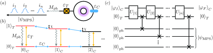
Figure 1: Generating photonic matrix product states (MPS) with circuit QED. (a) We consider a cavity dispersively coupled to a transmon, which can be controlled by driving both the cavity ($\varepsilon_{C}$) and the transmon ($\varepsilon_{T}$). The transmon excitation can be converted into a traveling microwave photon. By sequentially applying unitary operations followed by photon emissions $M_{\rm ph}$, one can produce a chain of entangled photons. (b) The level diagram of the system. The red (gray) levels are used in the protocol for $D=2$ MPS generation. The yellow (light gray) arrows denote driving of the transmon, and the blue (dark gray) arrows denote driving of the cavity. (c) Quantum circuit of the MPS generation protocol. The SWAP gates correspond to photon emissions ($M_{\rm ph}$).

Since rp-PEPS is a large class, our platform allows one to create photonic states useful for applications in quantum computing Hein et al. (2004); Takeuchi et al. (2019), metrology Jarzyna and Demkowicz-Dobrzański (2013); Koczor et al. (2020); Chabuda et al. (2020), communication and networking Azuma et al. (2015), as well as states that exhibit topological order Soejima et al. (2020); Verstraete et al. (2006); Buerschaper et al. (2009); Schuch et al. (2010). Moreover, the sequential nature of the protocol leads to temporally seperated microwave photons, which would allow one to efficiently distribute them to multiple receivers, thus directly building a multi-party entangled state. Realization of state transfer and distribution between superconducting quantum processors are intensely pursued currently Axline et al. (2018); Kurpiers et al. (2018); Magnard et al. (2020).

The rest of the article is structured as follows. In section II, we present our setup to generate arbitrary MPS using a microwave cavity coupled to a transmon qubit, discuss the imperfections that arise during the MPS generation, and estimate the performance of the device. In section III, we present the setup to generate photonic rp-PEPS and provide the circuits for generating the two-dimensional cluster state, the toric code, and isometric tensor network states. Finally, we analyze the scaling of the state preparation fidelity. We summarize our work in section IV.

II Generating MPS with cQED

In this section, first we introduce the setup in section II.1 and the MPS generation protocol in section II.2. Then we analyze the imperfections during the protocol in section II.3, and show in section II.4 that this protocol can be implemented using current technology.

II.1 cQED sequential photon source

We consider the setup sketched in Fig. 1(a), where a cavity (with the Hilbert space ${\cal H}_{C}$) is dispersively coupled to a transmon qubit (with the Hilbert space ${\cal H}_{T}$), with a Hilbert space ${{\cal H}_{{\rm{src}}}}={{\cal H}_{T}}\otimes{{\cal H}_{C}}$ Reagor et al. (2016). The transmon ground (excited) state is denoted by ${\left|0\right\rangle_{T}}$ (${\left|1\right\rangle_{T}}$). Defining the transition operator ${\sigma_{\alpha\beta}}={\left|\alpha\right\rangle_{T}}\left\langle\beta\right|$ for the transmon, the system Hamiltonian $H_{\rm src}(t)=H_{0}+H_{\rm drive}(t)$ contains a static part

$$H_{0}=\omega_{T}\sigma_{11}+\omega_{C}a^{\dagger}a-\chi\sigma_{11}a^{\dagger}a,$$ (2)

and time-dependent driving of transmon and cavity

$$H_{\text{drive }}(t)=\varepsilon_{C}(t)a+\varepsilon_{T}(t)\sigma_{01}+\text{ H.c. }$$ (3)

Here $\omega_{T}$ $(\omega_{C})$ is the frequency of the transmon qubit (cavity), and $a$ is the lowering operator of the cavity mode. The dispersive interaction strength $\chi$ sets a timescale for cavity-transmon gates. The driving amplitude of the qubit (cavity) is $\varepsilon_{T}$ $(\varepsilon_{C})$. The level structure of this system is shown in Fig. 1(b) . This Hamiltonian gives universal control of the cavity-transmon system Strauch (2012); Krastanov et al. (2015). We assume that one can engineer the following on-demand photon emission process $M_{\rm ph}$ from the transmon excitation

$$M_{\rm ph}\mathrel{\mathop{\mathchar 58\relax}}\quad|i\rangle_{T}\rightarrow|0\rangle_{T}|i\rangle_{\mathrm{ph}},\quad i=0,1.$$ (4)

For example, one can realize $M_{\rm ph}$ by coupling the qubit to an emitter via a tunable coupler Besse et al. (2020).

II.2 MPS generation protocol

The setup in section II.1 can sequentially generate photonic MPS using the generic protocol proposed in Ref. Schön et al. (2005), schematically shown in Fig. 1(c). We identify the first $D$ Fock states of the cavity mode as our basis for the $D$-level ancilla, with a Hilbert space $\cal{H}_{D}$. The MPS generation protocol starts from an ancilla initial state $\left|\varphi_{I}\right\rangle_{C}\in\mathcal{H}_{D}$ with the transmon in its ground state. In each photon generation round, the ancilla first interacts with the transmon, described by a unitary operation $U_{[i]}$. Then, the transmon emits its excitation and returns to its ground state (denoted by a SWAP gate in Fig. 1c), generating a photonic qubit defined by the presence or absence of a photon at that time.

Compared to the setup in Ref. Schön et al. (2007) which proposes to employ a $D$-level atom as ancilla and an optical cavity as emitter, our setup is better suited to current circuit QED experiments. In particular, our protocol exploits the long coherence times that can be achieved in microwave cavities and uses transmon qubits only to control and emit, but not to store excitations.

Throughout the protocol, unitaries are applied only after emission of the photon from the emitter, such that they always act on ancilla-transmon states of form $|\varphi\rangle_{C}|0\rangle_{T}$. As a result we can specify the action of the unitaries in terms of isometries $V$ that act only on the cavity Hilbert space

$$U_{[i]}\left(|\varphi\rangle_{C}|0\rangle_{T}\right)=\sum_{j=0}^{1}(V_{[i]}^{j}|\varphi\rangle_{C})|j\rangle_{T},$$ (5)

Since $U_{[i]}$ is unitary, the matrices $\{V_{[i]}^{j}\}$ satisfy the isometry condition $\sum_{j=0}^{1}V_{[i]}^{j\dagger}V_{[i]}^{j}=I_{D}$. The quantum state after $n$ rounds of photon generation is $|\Psi\rangle=M_{\rm ph}U_{[n]}\ldots M_{\rm ph}U_{[1]}\left|\varphi_{I}\right\rangle_{C}$. By disentangling the ancilla and the photonic state in the last step, we obtain the final state $|\Psi\rangle=\left|\varphi_{F}\right\rangle_{C}\otimes\left|\psi_{\mathrm{MPS}}\right\rangle$, which includes the following photonic MPS Schön et al. (2005)

$$\left|\psi_{\mathrm{MPS}}\right\rangle\propto\sum_{i_{1}\ldots i_{n}=0}^{1}{{}_{C}}\langle\varphi_{F}|V_{[n]}^{i_{n}}\ldots V_{[1]}^{i_{1}}|\varphi_{I}\rangle_{C}\left|i_{n}\ldots i_{1}\right\rangle.$$ (6)

We use the quantum optimal control (QOC) Wei et al. (2021); Machnes et al. (2018) to find the pulse sequences that implement the desired unitary operations for our protocol (see details in Appendix A). As a demonstration, we show how to generate a linear cluster state Briegel and Raussendorf (2001), which can be written as an MPS of bond dimension $D=2$, where

$$\begin{array}[]{l}V_{[i]}^{0}=\frac{1}{\sqrt{2}}\left(\begin{array}[]{ll}1&0\\ 1&0\end{array}\right),\quad V_{[i]}^{1}=\frac{1}{\sqrt{2}}\left(\begin{array}[]{cc}0&1\\ 0&-1\end{array}\right),\\ \left|\varphi_{I}\right\rangle_{C}=\frac{1}{\sqrt{2}}(|0\rangle+|1\rangle),\quad\left|\varphi_{F}\right\rangle_{C}=|0\rangle.\end{array}$$ (7)

In each round except the last, we apply the same unitary $U_{[i\neq n]}$ followed by photon emission represented by $M_{\rm ph}$, which adds one site to the state. In the last step, we apply the unitary $U_{[n]}$ followed by $M_{\rm ph}$, which emits the last photon and disentangles the source from the photons. The pulse sequence of the driving [Eq. 3] for implementing the two unitaries is shown in Fig. 2, and we provide more details in Appendix A.

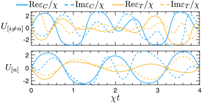
Figure 2: Optimized cavity and transmon drive [Eq. 3] to implement the unitaries $U_{[i\neq n]}$ and $U_{[n]}$ for the cluster state [Eq. 7] generation.

II.3 Analysis of experimental imperfections

Ideally, the above protocol would generate the desired pure photonic state $\left|{{\psi_{\rm MPS}}}\right\rangle$. However, various errors may occur in this system during the unitary operation and the photon emission process. Thus the protocol produces a $n$-photon density matrix $\rho_{\rm ph}$, with a non-unit fidelity ${{\cal F}_{{\rm{MPS}}}}={}_{\rm ph}\langle{{\psi_{{\rm{MPS}}}}}|{\rho_{{\rm{ph}}}}{|{{\psi_{{\rm{MPS}}}}}\rangle_{{\rm{ph}}}}$. Due to the sequential nature of the protocol, ${\mathcal{F}_{\rm MPS}}$ is an exponentially decaying function of the emitted photon number $n$, that is

$${{\cal F}_{{\rm{MPS}}}}={e^{-\xi\cdot n}},$$ (8)

where $\xi$ is the error per photon emission. An example of this behavior is shown in Fig. 3(a).

Decoherence processes in the cavity-transmon system include transmon decay at a rate ${\Gamma_{T}}$, cavity mode decay at a rate ${\Gamma_{C}}$, and transmon dephasing at a rate ${\Gamma_{\phi}}$ Heeres et al. (2017) . These processes happen both during the unitary operations and the photon emission process. The finite anharmonicity $\alpha$ of the transmon further allows leakage into the second excited state $|2\rangle_{T}$ in every unitary operation.

To model the imperfections due to finite anharmonicity $\alpha$ during unitary operations, we model the transmon as a truncated anharmonic oscillator with basis $\{{{{|0\rangle}_{T}},{{|1\rangle}_{T}},{{|2\rangle}_{T}}}\}$. After further including the decoherence effects, the system density matrix ${\rho_{{\rm{src}}}}\in{\cal H}_{\rm src}$ evolves under the master equation

$${{\dot{\rho}}_{{\rm{src}}}}(t) =-i[{{H^{\prime}_{{\rm{src}}}}(t),{\rho_{{\rm{src}}}}(t)}]$$ (9)

$$+\sum\limits_{n=T,C,\phi}{({{J_{n}}{\rho_{{\rm{src}}}}(t)J_{n}^{\dagger}-\frac{1}{2}\{{{\rho_{{\rm{src}}}}(t),J_{n}^{\dagger}{J_{n}}}\}})},$$

with $H^{\prime}_{{\rm{src}}}(t)$ being the system Hamiltonian including transmon double excitations with anharmonicity $\alpha$. Defining the spin operators ${\sigma_{ij}}={|i\rangle_{T}}\langle j|$, the jump operators are ${J_{T}}=\sqrt{{\Gamma_{T}}}({{\sigma_{01}}+\sqrt{2}{\sigma_{12}}}),{J_{C}}=\sqrt{{\Gamma_{C}}}a$, ${J_{\phi}}=\sqrt{{\Gamma_{\phi}}}({{\sigma_{11}}+2{\sigma_{22}}})$.

Since current experiments generally have $|\alpha|\gg|\chi|\gg{\Gamma_{C}},{\Gamma_{T}},{\Gamma_{\phi}}$ Reagor et al. (2016); Heeres et al. (2017); Chou et al. (2018), for a gate time $T\sim 1/|\chi|$ we can estimate the scale of the errors on ${{\cal F}_{{\rm{MPS}}}}$ during each unitary operation perturbatively. The total error $\xi$ is a sum of several parts: (i) transmon decay ${\xi_{{\Gamma_{T}}}}$, (ii) transmon dephasing ${\xi_{{\Gamma_{\phi}}}}$, (iii) cavity decay ${\xi_{{\Gamma_{C}}}}$, and (iv) transmon non-linearity ${\xi_{{\alpha}}}$. These contributions scale as

$$\begin{array}[]{*{20}{l}}{{\xi_{{\Gamma_{T}}}}\sim{\Gamma_{T}}/|\chi|,\qquad{\xi_{{\Gamma_{\phi}}}}\sim{\Gamma_{\phi}}/|\chi|,}\\ {{\xi_{{\Gamma_{C}}}}\sim{\Gamma_{C}}/|\chi|,\qquad{\xi_{\alpha}}\sim{|\chi|^{2}}/{|\alpha|^{2}}.}\end{array}$$ (10)

Imperfections also affect the photon emission process. First, there is a finite photon retrieval efficiency $p_{\rm em}$ of the emitter  associated to $M_{\rm ph}$. Second, system decoherence happens during the photon emission. We assume a finite photon emission rate $\Gamma_{\rm em}$, and thus a finite duration of photon emission ${T_{\rm em}}$ (which we can tune). In the regime of ${\Gamma_{T}},{\Gamma_{\phi}},{\Gamma_{C}}\ll{\Gamma_{\rm em}}$, we can estimate scaling of error on ${\cal F}_{{{\rm MPS}}}$ due to system decoherences during each emission process as

$$\begin{array}[]{l}\xi_{{\Gamma_{C}}}^{{\rm{em}}}\sim{\Gamma_{C}}T_{\rm em},\qquad\xi_{{\Gamma_{T}}}^{{\rm{em}}}\sim{\Gamma_{T}}/{\Gamma_{{\rm{em}}}},\\ \xi_{{\Gamma_{\phi}}}^{{\rm{em}}}\sim{\Gamma_{\phi}}/{\Gamma_{{\rm{em}}}},\qquad{\xi_{{p_{\rm em}}}}\sim-\log{p_{\rm em}}.\end{array}$$ (11)

Notably, here $\xi_{{\Gamma_{T}}}^{\rm em}$ and $\xi_{{\Gamma_{\phi}}}^{\rm em}$, which are due to transmon decoherence, do not depend on the emission time $T_{\rm em}$. The expression for $\xi_{{p_{\rm em}}}$ comes from the fact that ${e^{-{\xi_{{p_{{\rm{em}}}}}}{n_{{\rm{ph}}}}}}\sim p_{{\rm{em}}}^{{n_{{\rm{ph}}}}}$. The finite photon emission time also results in a residual population of the transmon first excited state ${p_{1T}}(T_{\rm em})={e^{-\Gamma_{\rm em}{T_{\rm em}}}}\cdot{p_{1T}}(0)$, which reduces the photon retrieval efficiency $p_{\rm em}$. The whole photon emission process including all imperfections can be described by a process map ${W_{\rm ph}}\mathrel{\mathop{\mathchar 58\relax}}{\cal H}_{\rm src}\to{\cal H}_{\rm src}\otimes{{\cal H}_{\rm ph}}$ that maps ${\rho_{\rm src}}$ to a system-photon joint density matrix (see the construction of $W_{\rm ph}$ in Appendix C). Finally, note that we did not include the imperfections during photon transmission, which is not a part of our model.

Using the solution of Eq. 9 and the process map ${W_{\rm ph}}$, we can use a matrix product density operator (MPDO) approach Wei et al. (2021) to obtain the photonic state fidelity ${\mathcal{F}_{\rm MPS}}$ and extract the overall error rate $\xi$ (details in Appendix B). As a demonstration, we analyze the process of generating the one-dimensional cluster state using the pulses in Fig. 2. From the scaling data of $\xi$ as a function of various imperfections (details in Appendix D), in the regime of small error ($\xi\ll 1$), we have

$$\xi\approx{\xi_{{\rm{unit}}}}+\xi_{{\rm{em}}}^{{\rm{src}}}+\xi_{{\rm{em}}}^{{\rm{ph}}},$$ (12)

which includes imperfections during unitary operation

$${\xi_{{\rm{unit}}}}={\beta_{0}}+\frac{{{\beta_{C}}{\Gamma_{C}}+{\beta_{T}}{\Gamma_{T}}+{\beta_{\phi}}{\Gamma_{\phi}}}}{{|\chi|}}+\frac{{{\beta_{\alpha}}\cdot|\chi{|^{2}}}}{{|\alpha{|^{2}}}},$$ (13)

cavity-transmon decoherence during photon emission

$$\xi_{{\rm{em}}}^{{\rm{src}}}={{\beta_{\phi,{\rm{em}}}}{\Gamma_{\phi}}/{\Gamma_{{\rm{em}}}}+{\beta_{C,{\rm{em}}}}{\Gamma_{C}}}T_{\rm em},$$ (14)

and imperfections of the photon emission

$$\xi_{{\rm{em}}}^{{\rm{ph}}}=-{\beta_{{\rm{em}}}}\log\left({(1-{e^{-{\Gamma_{\rm em}T_{\rm em}}}})\frac{{{\Gamma_{{\rm{em}}}}}}{{{\Gamma_{{\rm{em}}}}+{\Gamma_{T}}}}{p_{{\rm{em}}}}}\right).$$ (15)

The above overall scaling matches our qualitative prediction [Eqs. 10 and 11] very well. The non-universal coefficients $\{{{\beta_{i}}}\}$ depend on the target photonic state and the pulse shape, and are extracted from scaling data shown in Appendix C. In our example of cluster state generation, using the pulses shown in Fig. 2, we obtain

$$\begin{array}[]{l}{\beta_{C}}={\rm{2.20}},\quad{\beta_{T}}={\rm{1.43,}}\quad{\beta_{\phi}}={\rm{0}}.{\rm{92}},\\ {\beta_{\phi,{\rm em}}}={\rm{0.51,}}\quad{\beta_{{\rm{C}},{\rm{em}}}}={\rm{0.47,}}\quad{\beta_{{\rm{em}}}}={\rm{0.47}},\\ {\beta_{0}}={\rm{2}}.{\rm{58}}\times{\rm{1}}{{\rm{0}}^{-4}},\quad{\beta_{\alpha}}{\rm{=46}}.{\rm{7}}.\end{array}$$ (16)

Here ${\beta_{0}}$ corresponds to the imperfect synthesis of the optimal control pulse, and can typically be made negligible. All other $\{{{\beta_{i}}}\}$ are of order $O(1)$, except ${\beta_{\alpha}}$ which correspond to the effect of transmon double excitations, which is particularly large because it scales with the maximum driving amplitude of the transmon, which can be several times larger than $|\chi|$ (cf. Fig. 2). Note that the decoherence due to transmon double excitations [cf. Eq. 13] is still relatively small, thanks to the strong anharmonicity $|\alpha|$ that suppress the transmon double excitations, and one can further reduce this leakage error by including higher levels in the pulse optimization Rebentrost and Wilhelm (2009).

II.4 Performance estimation of protocol

We estimate the performance of this sequential photon source using current state-of-the-art experimental parameters. Specifically, we use cavity and transmon parameters Heeres et al. (2017) ${\Gamma_{C}}=$0.37\text{\,}\rm\mathrm{k}\mathrm{H}\mathrm{z}$$, ${\Gamma_{T}}=$5.88\text{\,}\rm\mathrm{k}\mathrm{H}\mathrm{z}$$, ${\Gamma_{\phi}}=$23.26\text{\,}\rm\mathrm{k}\mathrm{H}\mathrm{z}$$, $\alpha=2\pi\times-$236\text{\,}\rm\mathrm{M}\mathrm{H}\mathrm{z}$$, $\chi={\rm{2}}\pi\times-$2.194\text{\,}\rm\mathrm{M}\mathrm{H}\mathrm{z}$$, and the photon emission parameters Besse et al. (2020) ${\Gamma_{\rm em}}=2\pi\times$1.95\text{\,}\rm\mathrm{M}\mathrm{H}\mathrm{z}$$, $p_{\rm em}=1$ . We choose the photon emission duration as $T_{\rm em}^{\rm opt}=\log(1+{\beta_{{\rm{em}}}}{\Gamma_{{\rm{em}}}}/{\beta_{{\rm{C}},{\rm{em}}}}{\Gamma_{C}})/{\Gamma_{\rm em}}$ to minimize $\xi$ [cf. Eq. 12] under the assumption of a fixed photon emission rate ${\Gamma_{\rm em}}$. For the one-dimensional cluster state generated using the pulse sequence in Fig. 2, we plot the resulting fidelity ${\cal F}_{\rm MPS}$ in Fig. 3(a). Defining the entanglement length ${N_{\rm ph}}=\log 2/\xi$ (which $\xi$ has been defined in Eq. 8), which is the photon number at which the fidelity drops down to ${\cal F}_{\rm MPS}=1/2$, we obtain ${N_{\rm ph}}\approx 123$, which would mean an eightfold increase compared to the experimentally demonstrated ${N_{\rm ph}}\approx 15$ in Ref. Besse et al. (2020). This improvement partly comes from the fact that we exploit the long transmon lifetime reported in Ref. Heeres et al. (2017). If we use the transmon properties reported in Besse et al. (2020), our protocol gives ${N_{\rm ph}}\approx 47$ (see Appendix D), which is still a substantial improvement.

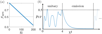
Figure 3: (a) The state fidelity versus the number of photons for the cluster state generated using the pulse sequence in Fig. 2, with the state-of-the-art parameters listed in section II.4. The horizontal line denotes ${\cal F}_{\rm MPS}=1/2$, with the corresponding photon number $N_{\rm ph}$ defined as the entanglement length of the photon string. (b) Evolution of the transmon excited population $p_{1T}$ during one sequence of cluster state generation. The $p_{1T}$ shows a transient evolution during the unitary operation $U_{[i\neq n]}$ driven by the pulse in Fig. 2, and exponentially decays during the photon emission process.

To understand this improvement, we plot the population $p_{1T}$ of the transmon excited state $|1\rangle_{T}$ during one photon generation round in Fig. 3(b). We see that $|1\rangle_{T}$ is only transiently populated during the unitary operation $U_{[i\neq n]}$ (driven by the pulse in Fig. 2), compared to the protocol in Ref. Besse et al. (2020) where one always has ${p_{1T}}=1/2$ during the cluster state generation. This leads to a substantial improvement of the entanglement length obtained in our protocol . Moreover, it is possible to further reduce $p_{1T}$ by adding a corresponding penalty in the optimal control algorithm (cf. Appendix A).

Finally, we estimate the scaling of $N_{\rm ph}$ with the bond dimension $D$ of the desired MPS as (see section D.3)

$${N_{{\rm{ph}}}}\propto{D^{-2}},$$ (17)

and this scaling mainly comes from the time $T_{\rm MPS}^{D}=O(D^{2})$ Lee et al. (2018a) taken to implement a unitary on the $2D$-dimensional Hilbert space $\dim{\cal H_{\rm src}}=2D$ (cf. section II.2). This scaling indicates that our system can create MPS of moderate bond dimensions. This already finds many applications and can efficiently capture the ground states of one-dimensional local gapped Hamiltonians Huang (a); Dalzell and Brandão (2019); Huang (b); Schuch and Verstraete .

III Generating rp-PEPS with cQED

The previous section shows that the proposed cavity-transmon system can produce high-fidelity one-dimensional photonic MPS. In this section, we demonstrate how to extend this to implement the high-dimensional photonic state generation protocol introduced in Ref. Wei et al. . First, in section III.1 we introduce the array of coupled sequential photon sources and prove the universality of the Hamiltonian for this system, which allows this system to implement arbitrary local unitary transformations. Then we show in section III.2 that, using this setup, one can generate radial plaquette PEPS (rp-PEPS), whose source point (cf. section III.2) sits on a corner of the lattice. After that, in section III.3 we demonstrate this protocol by discussing the preparation of two-dimensional cluster state, the toric code, and the isometric tensor network states (isoTNS). Finally, we analyze the scaling of the state preparation fidelity for this protocol in section III.4. Here we mainly focus on generating two-dimensional photonic states, however, this protocol readily extends to higher spatial dimensions Wei et al. .

III.1 Setup: array of sequential photon sources

Let us consider a natural generalization of the setup in section II.1 to a quasi-one-dimensional array of $L_{c}\times m$ cavity-transmon pairs, and use the first $D^{\prime}$ Fock states of each cavity. The $L_{c}$ cavities in each row form an ancilla $A$ of dimension $D=D{{}^{\prime{L_{c}}}}$. While $L_{c}=1$ is the most straightforward choice, sometimes it may be beneficial to choose $L_{c}>1$, as we comment on in section III.4. Moreover, in each row there is one emitter ${\{{{T_{j}}}\}_{j=1,...,m}}$ (see Fig. 4a), while other transmon qubits are used to provide universal control to the corresponding cavities .

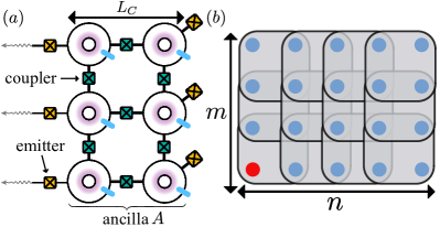
Figure 4: (a) The setup to generate photonic radial plaquette PEPS (rp-PEPS), which consist a quasi-one-dimensional array of cavity-transmon pairs (the notations follow that in Fig. 1a). In each row there is a transmon emitter that can emit photons. The neighboring cavities are connected by Y-shape couplers [the green (dark gray) boxes]. (b) rp-PEPS with open boundary conditions are produced by sequential applying unitaries on overlapping regions. Here the source point Wei et al. of the state is denoted by the red dot.

We couple each neighboring pair of photon sources by a coupler that interacts with both cavities Wang et al. (2016) (shown as green boxes in Fig. 4a). By driving the coupler with two-tone pumps, the four-wave mixing process of the coupler reduces to the following bilinear interaction Gao et al. (2018)

$$H_{{\rm{int}}}^{ij}(t)={g_{ij}}(t)({{e^{i{\varphi_{ij}(t)}}}a_{i}^{\dagger}{{a}_{j}}+{\rm H.c.}}).$$ (18)

Here $a_{i}^{\dagger}$ denote the creation operator of the cavity for $i$-th photon source. The coupling strength $g_{ij}(t)$ and phase $\varphi_{ij}(t)$ can be controlled through drives. Let us denote the set of vertices of the array of sources in Fig. 4(a) as $\cal V$, where each vertex $v_{ij}$ connects the cavities of the $i$-th and $j$-th cavity-transmon pairs. One can thus write down the Hamiltonian of this system as

$${H_{{\rm{array}}}}(t)=\sum\limits_{i=1}^{{L_{c}}\times m}{H_{{\rm{src}}}^{i}(t)}+\sum\limits_{{v_{ij}}\in{\cal V}}{H_{{\rm{int}}}^{ij}}(t),$$ (19)

where $H_{\rm src}^{i}$ is the Hamiltonian for the $i$-th source, containing the terms in Eqs. 2 and 3. Equipped with the universal control of each source and the bilinear couplings, we prove in Appendix F that $H_{\rm{array}}$ provides universal control. Given this, we can assume that one can implement arbitrary local unitary operations one this system.

In sum, this system can be represented by a one-dimensional array of $D{{}^{\prime{L_{C}}}}$-level ancillas (labeled by ${\{{{A_{j}}}\}_{j=1,...,m}}$) coupled to transmon emitters (labeled by ${\{{{T_{j}}}\}_{j=1,...,m}}$), illustrated in Fig. 5. Note that one can let more transmons in each row to emit photons, which effectively increase the dimension of the transmon emitters. Finally, in the next sections we will treat each ancilla effectively as $L_{p}-1$ qubits by choosing $D^{\prime}$ and $L_{c}$ such that

$$D{{}^{\prime{L_{C}}}}\geq{2^{{L_{p}}-1}}.$$ (20)

III.2 Preparation of rp-PEPS

Ref. Wei et al. introduces a generic protocol to produce rp-PEPS on flying qubits. rp-PEPS are states prepared by sequentially applying unitaries on plaquettes of size $L_{p}\times L_{p}$ ($L_{p}\ll n,m$) in a radial fashion [see Fig. 4(b) for an example]. They possess long-range correlations and area-law entanglement, and photonic rp-PEPS can be efficiently prepared with the circuit depth Eq. 1.

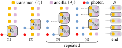
Figure 5: The preparation of photonic rp-PEPS ($L_{p}=2$ here). In the preparation of the $(i,j)$-th site, we apply a unitary ${\hat{U}_{[{i,j}]}}$ followed by a photon emission of the transmon $T_{j}$. After the initial steps (1) and (2), steps (3) and (4) will be repeated. At the end of the protocol, we swap the excitations on the ancillas to the emitters and then convert them to photons, denoted as $\cal S$.

The generation procedure of rp-PEPS is shown in Fig. 5. We start from an initial state where all the cavities and the transmons are in their ground states $|{{\varphi_{0}}}\rangle=|{{0_{\{{{A_{j}}}\}}}}\rangle\otimes|{{0_{\{{{T_{j}}}\}}}}\rangle$, and sequentially apply unitaries $\{{{{\hat{U}}_{\left[{i,j}\right]}}}\}$. The unitary $U_{[i,j]}$ is applied in the $i$-th layer on the ancillas $\{{{A_{j}},...,{A_{j+{L_{p}}-1}}}\}$ and transmons $\{{{T_{j}},...,{T_{j+{L_{p}}-1}}}\}$. As each ancilla can be viewed effectively as $L_{p}-1$ qubits Eq. 20, the unitary equivalently acts on a plaquette of qubits of size $L_{p}\times L_{p}$. After each unitary, we trigger the photon emission from the transmon $T_{j}$ (denoted as isometry $M^{j}_{{\rm{ph}}}$ [cf. Eq. 4]). Note that after the last unitary per column, the last emission process per column $M^{m-L_{p}+1}_{{\rm{ph}}}$ (see step 4 of Fig. 5) convert excitations of transmons $\{{{T_{m-{L_{p}}+1}},...,{T_{m}}}\}$ to multiple photonic qubits at the same time. Repeatedly applying this procedure following the order shown in Fig. 5 (also see the below Eq. 21), and in the end emitting the remaining excitations in the ancillas (an operation collectively denoted as $\cal S$), we generate the desired two-dimensional photonic state Wei et al.

$$|{\psi_{{\rm{rp}}}}\rangle=\langle\varphi_{0}|{\cal S}\prod\limits_{i=1}^{n-L_{p}+1}{\prod\limits_{j=1}^{m-L_{p}+1}{(M_{{\rm{ph}}}^{j}{{\hat{U}}_{[i,j]}})}|\varphi_{0}\rangle}.$$ (21)

Given the universal control of Eq. 19, this protocol can produce arbitrary states of form Eq. 21 (schematically shown in Fig. 4b), which are two-dimensional rp-PEPS of plaquette size $L_{p}$ with open boundary condition, with their source point located at the first photon being created . Also note that, in the above protocol, photon emissions reset the transmon. This allows one to efficiently reuse them, and this parallelize the preparation procedure (shown in steps 3 and 4 of Fig. 5), such that the circuit depth for preparing rp-PEPS of plaquette length $L_{p}$ on a $n\times m$ lattice asymptotically scales as Eq. 1 Wei et al. . This system further allows increasing the plaquette size by increasing the number of cavity-transmon pairs $L_{C}$ or using more modes $D^{\prime}$ in the cavity.

Finally, we note that by replacing the photon emissions with qubit measurements, this state generation protocol naturally becomes a qubit-efficient quantum variational scheme Huggins et al. (2019); Liu et al. (2019).

III.3 Examples

III.3.1 Two-dimensional cluster state

Consider a two-dimensional square lattice, with the position vector of each site denoted as $\vec{a}\equiv\left({i,j}\right)$. The two-dimensional cluster state ${|{\rm Cl}\rangle_{{\rm{2D}}}}$ is prepared starting from a product state of all qubits in $\left|+\right\rangle$ by applying control-Z (CZ) gates on each nearest-neighbour pairs of qubits Briegel and Raussendorf (2001)

$${|{\rm Cl}\rangle_{{\rm{2D}}}}={\prod\limits_{\vec{b}{\textrm{ adjacent }}\vec{a}}{{\rm{C}}{{\rm{Z}}_{\vec{a}\vec{b}}}}}\textrm{ }\mathop{\bigotimes}\limits_{\left\{{\vec{a}}\right\}}\left|+\right\rangle.$$ (22)

This state is an rp-PEPS of plaquette size $L_{p}=2$, thus it can be prepared by the protocol in section III.2, where each ancilla consists of a qubit (this means that we use $L_{c}=1$ cavity with $D^{\prime}=2$ Fock basis). The preparation procedure is shown in Fig. 6, where the corresponding plaquette unitaries $\{{{U_{\left[{i,j}\right]}}}\}$ in Eq. 21 are formed by CZ, SWAP, and Hadamard gates.

One can easily extend the size of the state horizontally by repeatedly applying the steps 5.1-8 in Fig. 6, and vertically by fabricating a longer chain of ancilla-transmon pairs. Moreover, omitting some photon emissions, one can create arbitrary graph states of local connectivities in this way Russo et al. (2019).

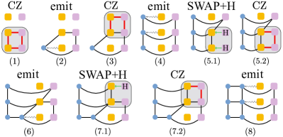
Figure 6: Preparing two-dimensional cluster state ${|{\rm Cl}\rangle_{{\rm{2D}}}}$ following the rp-PEPS preparation protocol (cf. Fig. 5, and we keep the same notation as there). Here both the ancillas and transmons have two levels (qubits), initialized in the state $|+\rangle$. The lines connecting two qubits mean that they have been acted on by a control-Z (CZ) gate in a previous step, whereas the thick red (gray) lines denotes that CZ gates are being applied in that step. The steps from 1 to 4 prepare the first column of photons. To create the next column of photons, in each unitary we first swap certain ancilla states to the corresponding transmons in the same row [illustrated by green (gray) arrows], then apply Hadamard gates to set the ancilla states to $\left|+\right\rangle$ (see 5.1 and 7.1), and finally before apply CZ gates, which prepares the second column (see step 8). By repeating steps 5.1 to 8, one can prepare ${|{\rm Cl}\rangle_{{\rm{2D}}}}$ of arbitrary size.

To prepare ${|{\rm Cl}\rangle_{{\rm{2D}}}}$ of size $n\times m$, the depth for this circuit in terms of plaquette unitaries is ${\cal T}\approx 2n+m$ [cf. Eq. 1]. We also point out that this can be further improved to ${\cal T_{\rm cl}}\approx 2n$, since the CZ gates commute with each other. As an example, steps 1-4 in Fig. 6 can be combined such that we apply CZ gates on all adjacent pairs in the ancilla-transmon array in parallel (which are contained in two layers of plaquette unitaries), then emit one column of photons. The CZ gates between two cavities can be realized by combining single-qubit rotations and a CNOT gate, which has been experimentally implemented in Ref. Rosenblum et al. (2018).

The above further parallization of the circuit show a generic feature of photonic rp-PEPS [Eq. 21]: if the sequential product of unitaries $\hat{U}_{{\rm{col}}}^{i}=\prod\nolimits_{j=1}^{m-{L_{p}}+1}{{{\hat{U}}_{\left[{i,j}\right]}}}$ for preparing each column of photons can be parallelized as a circuit of depth $O(1)$, one can directly implement $\hat{U}_{{\rm{col}}}^{i}$ followed by the photon emission of all transmon emitters $\mathop{\otimes}\limits_{j}M_{{\rm{ph}}}^{j}$ to prepare the $i$-th column of the rp-PEPS. This also applies to the toric code below.

III.3.2 The toric code

The toric code Dennis et al. (2002); Kitaev (2003) is an example of a string-net state, and finds important applications in quantum error correction. It is defined as the simultaneous $+1$ eigenstate of all star operators $A_{s}=\prod_{i\in s}Z_{i}$ (green boxes in Fig. 7a) and plaquette operators $B_{p}=\prod_{j\in p}X_{j}$ (red boxes in Fig. 7a), i.e. $A_{s}|{{\rm{TC}}}\rangle=B_{p}|{{\rm{TC}}}\rangle=+1|{{\rm{TC}}}\rangle$. Here $\{Z_{i}\}$ and $\{X_{j}\}$ are Pauli operators.

The toric code has recently been prepared on a stationary lattice, with the following procedure J. et al. (2021)

1. Initialize the whole lattice in the state $\mathop{\bigotimes}\limits_{\left\{{\vec{a}}\right\}}\left|0\right\rangle$, where all $\langle{{A_{s}}}\rangle=1$ and $\langle{{B_{p}}}\rangle=0$.

2. Choosing a qubit for each plaquette as the representative qubit (an example choice is denoted by purple dots in Fig. 7a), and apply Hadamard gate on it.

3. Within each plaquette, sequentially apply CNOTs with the representative qubit as the control and other qubits as targets, with an ordering such that the representative qubits are not changed until the CNOTs in their plaquette have been applied [cf. Fig. 7(b)].

Inspired by this procedure, one can prepare $|{\rm TC}\rangle$ as a photonic rp-PEPS of $L_{p}=2$ using the protocol in section III.2, with each ancilla consisting of a single qubit. To ease the notation, in Fig. 7(b) we group the gates in steps 2-3 of the above procedures that act on each plaquette as $\hat{V}$, and the gates used to swap the ancilla and transmon state as ${\hat{S}_{u}}$ and ${\hat{S}_{ud}}$.

Figure 7: Preparation of photonic toric code $|{\rm TC}\rangle$, inspired by Ref. J. et al. (2021). Throughout this figure, we keep the same notation as that in Fig. 5. The support of the star operators $A_{s}$ is shown in green (light gray), and that of the plaquette operators $B_{p}$ in red (dark gray). (a) The toric code is the unique $+1$ eigenstate of all star and plaquette operators $A_{s}$ and $B_{p}$. Each plaquette has a ‘representative qubit’, denoted by a purple dot. (b) We group the Hadamard and CNOT gates that will be applied to each plaquette as $\hat{V}$. The SWAP gates are denoted as ${\hat{S}_{u}}$ and ${\hat{S}_{ud}}$. (c) We alternatively apply $\hat{V}$ or identity gate $I$ in each step (dashed lines separate different steps), followed by a photon emission (for example, from steps 1 to 3). Also after each photon emission, one needs to swap the corresponding ancilla state to the transmon, thus in steps 4-9 the unitaries are generally the product of swap gates (${\hat{S}_{u}}$ or ${\hat{S}_{ud}}$) with $\hat{V}$ or $I$. (d) After step 9 of the panel (c), one obtains $|{\rm TC}\rangle$ of size $4\times 4$ with the same geometry as that in panel (a), consisting of three columns of photonic qubits and the column of ancilla qubits. By further repeating the steps from 4-9 in panel (c) and using more ancilla-transmon pairs, one can generate $|{\rm TC}\rangle$ of arbitrary size.

The preparation circuit is shown in Fig. 7(c), where the plaquette unitaries are alternatively formed by $\hat{V}$ or the identity gate $\hat{I}$, and their product with swap gates (${\hat{S}_{u}}$ or ${\hat{S}_{ud}}$). The $\hat{V}$ implement desired operations for each toric code plaquette region J. et al. (2021), while the photon emission and swap gates will ‘push’ the produced entangled states toward the photon lattice (denoted by blue circles). After all operations in Fig. 7(c), one obtains $|{\rm TC}\rangle$ of size $4\times 4$ on three columns of photonic qubits and the ancilla qubits, shown in Fig. 7(d). By further repeating the steps from 4-9 in Fig. 7(c) and using more ancilla-transmon pairs, one can generate $|{\rm TC}\rangle$ of arbitrary size. We also point out that, by further parallelizing the unitaries J. et al. (2021), one can apply the same procedure as described in the two-dimensional cluster state generation protocol [cf. section III.3.1] to obtain a circuit depth ${{\cal T}_{\rm TC}}\approx{2n}$ in terms of plaquette unitaries for generating $\left|{\rm TC}\right\rangle$ of size $n\times m$.

The schemes presented here for cluster state generation and toric code generation are directly derived from their circuit generation on stationary lattices. This idea allows one to obtain photonic state generation circuits by utilizing existing circuits on stationary lattices. For example, one can generate string-net states by extending the protocol in section III.3.2, using similar circuits as in Ref. Liu et al. .

III.3.3 Isometric tensor network states

The rp-PEPS contain the isometric tensor network states Zaletel and Pollmann (2020) (isoTNS) as a subclass Wei et al. . An isoTNS is parametrized by its bond dimension $D$ Zaletel and Pollmann (2020) which bounds the entanglement entropy of the state, and its physical dimension $d$, which specifies the Hilbert space dimension of each site.

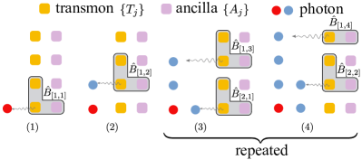
Figure 8: Preparation of isoTNS with bond dimension $D=2$ and physical dimenison $d=2$. In the preparation of the $(i,j)$-th site, we apply a unitary ${\hat{B}_{[{i,j}]}}$ connecting the cavity $C_{j}$ and the transmons $T_{j},T_{j+1}$, followed by a photon emission of the transmon $T_{j}$. After the initial steps (1 and 2), steps 3 and 4 will be repeated to build up the desired 2D isoTNS. The red (dark gray) dot denotes the orthogonality center of the isoTNS.

As the protocol in section III.2 can prepare rp-PEPS with the source point in the corner of the lattice, one can prepare the subclass of isoTNS whose orthogonality center (see details in Appendix E) is in this corner. To do so, one has to require the unitaries to have an ‘L’-shape Wei et al. , as shown in Fig. 8 for the case of $D=2$ and $d=2$. Here each unitary $\hat{B}_{[i,j]}$ acts on the ancilla $A_{j}$ and transmons $\{{{T_{j}},...,{T_{j+{L_{p}}-1}}}\}$ to produce isoTNS of bond dimension $D\leq 2^{L_{p}-1}$. Increasing isoTNS bond dimension corresponds to increasing the arm length of the ‘L’-shaped unitary. In the end of the protocol, we can disentangle the ancilla from the photonic state being produced Wei et al. . We provide more details on isoTNS in Appendix E.

The subclass of isoTNS whose orthogonality center is in the corner of the lattice already contains all graph states of local connectivities Russo et al. (2019) and all string-net states Soejima et al. (2020), and thus the two-dimensional cluster state and toric code discussed previously can be also created in this way. However, we point out that, the circuits we presented in sections III.3.1 and III.3.2 are more efficient than the circuit derived from their isoTNS representation. For example, the isoTNS representation of arbitrary $\mathbb{Z}_{\lambda}$ toric code Bullock and Brennen (2007) is shown in section E.1, where the physical dimension of the tensor is $\lambda^{4}$. Thus for the qubit ($\lambda=2$) toric code ($|{{\rm{TC}}}\rangle$ discussed in section III.3.2), this isoTNS generation scheme requires each transmon emitter to be 16-dimensional, for which we need to couple multiple transmons to the same ancilla, thus is more complex than the scheme shown in section III.3.2. The existence of isoTNS representation of $\mathbb{Z}_{\lambda}$ toric code for arbitrary $\lambda$ also implies that our scheme can create photonic qudit toric code, and such states show certain advantages as quantum error-correcting codes compared to the qubit toric code Duclos-Cianci and Poulin (2013); Watson et al. (2015).

Finally, isoTNS is a class of states that can be efficiently prepared as shown here (also see Ref. Wei et al. ), and serve as an ansatz for classical variational algorithms Zaletel and Pollmann (2020). Combining these two features may allow one to implement interesting protocols such as variational quantum metrology Jarzyna and Demkowicz-Dobrzański (2013); Koczor et al. (2020); Chabuda et al. (2020).

III.4 Scaling of rp-PEPS generation fidelity

In the presence of imperfections, the rp-PEPS generation protocol [cf. section III.2] will yield a mixed photonic state ${\rho_{\rm rp}}$. Here we provide a qualitative estimation of the fidelity ${{\cal F}_{\rm rp}}=\langle{{\psi_{\rm rp}}}|{\rho_{\rm ph}}|{{\psi_{\rm rp}}}\rangle$ of the rp-PEPS generation protocol. Moreover, one can calculate the fidelity exactly by extending the MPDO approach in Appendix B.

Let us consider the array shown in Fig. 5(b) with $m$ rows, where each row consists of $L_{C}$ cavity-transmon pairs, with each cavity and transmon having the decoherence channels described in section II.3. Since we use the first $D^{\prime}$ Fock states of the cavity, we take the worst-case estimation of the cavity decay rate ${\Gamma^{\prime}_{C}}=(D^{\prime}-1)\Gamma_{C}$.

To prepare a generic rp-PEPS of size $n\times m$ and plaquette length $L_{p}(L_{p}\ll n,m)$, when preparing each photon we need to apply a unitary acting on $L_{p}^{2}$ qubits, thus $\dim{{{\hat{U}}_{\left[{i,j}\right]}}}\approx 2^{L_{p}^{2}}$. We estimate the time $T_{\rm rp}$ of implementing a generic unitary using optimal control methods as $T_{\rm rp}\sim{({\dim{{\hat{U}}_{\left[{i,j}\right]}}})^{2}}=O({{4^{L_{p}^{2}}}})$ Lee et al. (2018a). Note that the numerical cost of the pulse optimization also increases exponentially with $L_{p}^{2}$. Since both the initial and the final state of the sources are the ground state $\left|{{\varphi_{0}}}\right\rangle$ [cf. Eq. 21], in the preparation procedure [cf. Fig. 5], each source remains excited for a time $L_{p}nT_{\rm rp}$. Moreover, there are in total around $nm$ photon emissions. Thus by applying the same argument as in the MPS generation protocol (cf. section II.3), one can estimate the scaling of the fidelity as

$${{\cal F}_{{\rm{rp}}}}\sim\exp\left[{-{\xi^{\prime}}^{D^{\prime}}_{{\rm{unit}}}\cdot m{L_{c}}\cdot{L_{p}}n{T_{\rm rp}}-({{\xi^{\prime}}_{{\rm{em}}}^{{{\rm src},D^{\prime}}}+{\xi^{\prime}}_{{\rm{em}}}^{{\rm{ph}}}})\cdot nm}\right],$$ (23)

with ${\xi^{\prime}}^{D^{\prime}}_{{\rm{unit}}}$, ${\xi^{\prime}}_{\rm em}^{{{\rm src},D^{\prime}}}$ and ${\xi^{\prime}}_{\rm em}^{\rm ph}$ of the same form as that in Eqs. 13, 14 and 15, but with cavity decay rate $\Gamma_{C}$ replaced by $\Gamma^{\prime}_{C}$ and different non-universal constants $\{{{\beta^{\prime}_{i}}}\}$.

Given $L_{p}$, the number of cavities in each ancilla $L_{C}$ is ${L_{C}}=\left\lceil{({{L_{p}}-1})/{{\log}_{2}}D^{\prime}}\right\rceil$. We can thus write overall scaling [Eq. 23] as ${\cal F}_{\rm rp}\sim\exp({-{\xi^{L_{p},D^{\prime}}_{\rm rp}}\cdot nm})$, with the error rate of generating each photon ${\xi^{L_{p},D^{\prime}}_{\rm rp}}$ as

$$\xi_{{\rm{rp}}}^{{L_{p}},D^{\prime}}\approx{4^{L_{p}^{2}}}({{L_{p}}-1}){L_{p}}\cdot{\xi^{\prime}}_{\rm unit}^{D^{\prime}}/{\log_{2}}D^{\prime}+{{\xi^{\prime}}_{\rm em}^{{{\rm src},D^{\prime}}}+{\xi^{\prime}}_{\rm em}^{\rm ph}}.$$ (24)

From the above analysis, we see that using more cavities $L_{c}>1$ reduces the maximum number of excitations in each cavity $D^{\prime}=\left\lceil{2^{(L_{p}-1)/L_{c}}}\right\rceil$ significantly, which leads to a corresponding reduction in the error due to cavity decay $\Gamma^{\prime}_{C}=(D^{\prime}-1)\Gamma_{C}$. In addition, it is experimentally easier to control cavities with small Hilbert space than controlling a single cavity with a large Hilbert space. However, the fidelity of the inter-cavity connection is generally lower than the single cavity operation Gao et al. (2018). So depending on the desired plaquette length $L_{p}$ of the rp-PEPS, one needs to choose appropriate $L_{c}$ and $D^{\prime}$ to get the highest possible fidelity. A precise determination of the optimal $L_{c}$ and $D^{\prime}$ further depends on the specific target state, the details of the unitary operations, as well as the errors in the inter-cavity operations Gao et al. (2018); Zhang et al. (2019).

We expect an experimental realization of the simplest $L_{c}=1$ protocol could be a good first step to further understand the performance of the rp-PEPS protocol. In the end, an experiment aiming at large plaquette sizes may have to be optimized regarding the total number of cavities used, but this is beyond the scope of the present paper.

IV Conclusion

We propose a physical platform and a protocol to sequentially generate microwave photonic tensor network states with moderately high bond dimensions based on a dispersively coupled cavity-transmon system. The good coherence properties of microwave cavities lead to favorable scaling of the photon number for the MPS, in particular, we show this platform can potentially create a one-dimensional cluster state of over a hundred photons deterministically with current technology. The good connectivity makes this platform a promising candidate for generating a large class of high-dimensional rp-PEPS, and we show how to create a two-dimensional cluster state, the toric code, and isoTNS as examples. Our work thus serves as systematic guidance for sequential photon generation experiments in circuit QED platforms, and can naturally be applied to other dispersively coupled qubit-oscillator systems.

Our work can be extended in many ways. First, there are plenty of ideas to further reduce the imperfections during the protocol by applying error-correction techniques Ofek et al. (2016); Campagne-Ibarcq et al. (2020), applying error-transparent gates or path-independent gates Ma et al. (2019) on the bosonic modes, or applying open system optimal control techniques Schulte-Herbrüggen et al. (2011); Machnes et al. (2018); Abdelhafez et al. (2019). Second, the ability to generate strongly correlated photonic tensor network states opens the door of developing quantum information processing protocols that go beyond MPS Jarzyna and Demkowicz-Dobrzański (2013); Chabuda et al. (2020); Koczor et al. (2020). One can further simultaneously use coupled arrays of emitters and non-Markovian feedback approaches Pichler et al. (2017); Dhand et al. (2018); Xu and Fan (2018); Wan et al. ; Zhan and Sun (2020); Shi and Waks ; Bombin et al. to reduce the component overhead of the system and possibly generate a larger class of photonic states.

Appendix A MPS generation with cQED using Quantum Optimal Control Approach

In this section, we introduce our quantum optimal control (QOC) approach (similar to that used in Wei et al. (2021)) to implement unitaries on this setup.

We aim to find the driving amplitude ${{\varepsilon_{C}}(t),{\varepsilon_{T}}(t)}$ for the control ${H_{\rm drive}}(t)$ [Eq. 3] that implements the desired unitary operations $U_{[i]}$ [Eq. 5] in ${{\cal H}_{D}}\otimes{{\cal H}_{T}}$.

Given the target MPS to be prepared [Eq. 6], one can construct a series of isometries $\{{{{\hat{A}}_{[i]}}}\}$ that needs to be implemented on the system Schön et al. (2005). For generating the $n$-photon cluster state [Eq. 7], this construction gives two kinds of isometries ${\hat{A}_{[{i\neq n}]}}$ and ${\hat{A}_{[{n}]}}$, as well as the ancilla initial state ${|{{\varphi_{I}}}\rangle_{C}}$ needed in the protocol [cf. Eq. 6]:

$$\begin{array}[]{*{20}{l}}{{{\hat{A}}_{[i\neq n]}}=\left(\begin{array}[]{l}V_{\left[i\right]}^{0}\\ V_{\left[i\right]}^{1}\end{array}\right)=\frac{1}{{\sqrt{2}}}\left({\begin{array}[]{*{20}{c}}1&0\\ 1&0\\ 0&1\\ 0&{-1}\end{array}}\right),\quad{{\hat{A}}_{[n]}}=\left({\begin{array}[]{*{20}{c}}1&0\\ 0&0\\ 0&1\\ 0&0\end{array}}\right),}\\ {|{\varphi_{I}}{\rangle_{C}}=\frac{1}{{\sqrt{2}}}{{(|0\rangle}_{C}}+|1{\rangle_{C}}).}\end{array}$$ (25)

Note that here ${{\hat{A}}_{[{n}]}}$ is different from all other ${{\hat{A}}_{[i\neq n]}}$, as it contains an additional operation to disentangle the cavity from the photons.

We can embed above $\{\hat{A}_{[i]}\}$ into ${U_{[i]}}$ to realize Eq. 5 [see below Eq. 26]. In numerical calculations we keep the first $N_{C}>D$ Fock states in ${\mathcal{H}}_{C}$. Thus $\dim{{\cal H}_{C}}={N_{C}}$ in our numerical calculation. One can then write $U_{[i]}$ as

$${{U}_{[i]}}=\left({\begin{array}[]{*{20}{c}}{{{\hat{A}}_{[i]}}}&{{B_{1}}}\\ O&{{B_{2}}}\end{array}}\right),$$ (26)

with its basis vector permuted as

$${\rm{Base}}(U_{[i]})\equiv[{{\rm{Base}}({{{\cal H}_{D}}\otimes{{\cal H}_{T}}}),{\rm{others}}}].$$ (27)

The $O$ is a zero matrix, which physically means that ${U_{[i]}}$ does not cause the population to leak out of ${{\cal H}_{D}}\otimes{{\cal H}_{T}}$. The parts $B_{1}$ and $B_{2}$ are arbitrary, as long as ${U_{[i]}}$ is a unitary of dimension $2N_{C}$. One needs two kinds of unitaries. Each application of ${U_{[{i\neq n}]}}$ followed by the photon emission adds one site to the cluster state. The last unitary ${U_{[{n}]}}$ followed by a photon emission disentangles the source from the photonic MPS.

To apply quantum optimal control (QOC) to our cQED platform with Hamiltonian $H_{\rm src}$ [Eqs. 2 and 3], we go to the rotating frame to remove energy terms of the transmon and the cavity mode in $H_{\rm src}$, getting

$${H^{\prime}_{{\rm{src}}}}(t)=\chi{\sigma_{11}}{a^{\dagger}}a+[{{\varepsilon_{C}}(t)a+{\varepsilon_{T}}(t){\sigma_{01}}+{\rm{H.c.}}}],$$ (28)

and readily apply the QOC algorithm in Ref. Wei et al. (2021) with the control Hamiltonian ${{H^{\prime}_{{\rm{src}}}}}(t)$ to find the pulse sequences to implement desired $U_{[i]}$. The pulse sequence to implement ${U_{[{i\neq n}]}}$ and ${U_{[{n}]}}$ for the cluster state generation are shown in Fig. 2, where we choose $N_{C}=5$.

Appendix B The Matrix Product Density Operator (MPDO) approach to compute state fidelity

In this section we recall the MPDO approach Wei et al. (2021) to compute the fidelity ${{\cal F}_{{\rm{\rm MPS}}}}$ of the photonic state. We can rewrite the master equation Eq. 9 in a vectorized form

$$\dfrac{{d{{\vec{\rho}}_{{\rm{\rm src}}}}(t)}}{{dt}}={\cal L}(t){\vec{\rho}_{{\rm{\rm src}}}}(t),\qquad{\vec{\rho}_{{\rm{\rm src}}}}=\sum\limits_{a,b=1}^{{N_{h}}}{{\rho_{ab}}}|{a\otimes\bar{b}}\rangle,$$ (29)

Here $\mathcal{L}(t)$ is the Liouville operator, $|a\rangle$ is a basis element in ${\cal H}_{\rm src}$ and $|\bar{a}\rangle$ represent its complex conjugate. The solution of Eq. 29 is

$${\vec{\rho}_{\rm{\rm src}}}(T)=\mathcal{T}\{{{e^{\int_{0}^{T}{\mathcal{L}(t)dt}}}}\}{\vec{\rho}_{\rm{\rm src}}}(0)={W_{\cal L}}{\vec{\rho}_{\rm{\rm src}}}(0).$$ (30)

The photon emission process can be described by a process map

$${W_{\rm ph}}=\sum\limits_{i,j=0}^{1}{\sum\limits_{a,b,c,d=1}^{N_{h}}{W_{P,abcd}^{ij}}}|{c,\bar{d},i,\bar{j}}\rangle|{a,\bar{b}}\rangle,$$ (31)

which maps ${\vec{\rho}_{{\rm{\rm src}}}}$ with vectorized basis $|{a,\bar{b}}\rangle$ to a system-photon joint density matrix with vectorized basis $|{c,\bar{d},i,\bar{j}}\rangle=|{c,\bar{d}}\rangle\otimes{|{i,\bar{j}}\rangle_{\mathrm{\rm ph}}}$. Thus each photon generation round results in a map from the joint density matrix ${\vec{\rho}_{[k-1]}}$ of $k-1$ photons and system to the joint density matrix ${\vec{\rho}_{[k]}}$ of $k$ photons and system:

$${\vec{\rho}_{[k]}}=\sum\limits_{{i_{k}},{j_{k}}=0}^{d-1}{N_{[k]}^{{i_{k}},{j_{k}}}{{\vec{\rho}}_{[{k-1}]}}},\qquad{\rm{with}}\quad N_{[k]}^{{i_{k}},{j_{k}}}=W_{\rm ph}^{{i_{k}}{j_{k}}}{W_{{{\cal L}_{[k]}}}}.$$ (32)

The fidelity ${{\cal F}_{\rm MPS}}$ can be efficiently evaluated as Wei et al. (2021)

$$\begin{array}[]{l}{{\cal F}_{{\rm{MPS}}}}=\sum\limits_{\{{{i_{k}},{j_{k}}}\}=0}^{1}{{\rm{Tr}}[{N_{[n]}^{{i_{n}},{j_{n}}}...N_{[1]}^{{i_{1}},{j_{1}}}\tilde{B}}]}\times{\rm{Tr}}[{({A_{[n]}^{{j_{n}}}\otimes\bar{A}_{[n]}^{{i_{n}}}})...({A_{[1]}^{{j_{1}}}\otimes\bar{A}_{[1]}^{{i_{1}}}})({B\otimes B})}],\end{array}$$ (33)

where we denote $\tilde{B}\equiv\sum\limits_{\alpha=1}^{N_{h}}{|{{\varphi^{\prime}_{I}}}\rangle\langle\alpha|\otimes|{{\varphi^{\prime}_{I}}}\rangle\langle\alpha|}$, $B\equiv|{{\varphi_{I}}}\rangle\langle{{\varphi_{F}}}|$, and $\bar{A}$ as the complex conjugate of a matrix $A$. For higher-dimensional rp-PEPS, the ${{\mathcal{F}}_{{\rm{rp}}}}$ can be computed in the same way by viewing the high-dimensional rp-PEPS as an MPS with bond dimension and physical dimension scale exponentially with the number of sequential photon sources $m$.

Appendix C Construction of process map $W_{\rm ph}$

The decoherence effects and the finite photon retrieval efficiency ${p_{\rm em}}$ during the photon emission will modify $W_{\rm ph}$ from its ideal form ${W_{\rm ph}}={M_{\rm ph}}\otimes{\bar{M}_{\rm ph}}$ with $M_{\rm ph}$ of the form Eq. 4. A good way to construct $W_{\rm ph}$ is to include environmental photon modes which capture the erroneous jump events. When there is a finite photon retrieval efficiency ${p_{\rm em}}$, we can include an environmental photon mode ${\varepsilon_{T}}$, and the ${M_{\rm ph}}\mathrel{\mathop{\mathchar 58\relax}}{{\cal H}_{T}}\to{{\cal H}_{T}}\otimes{{\cal H}_{\rm ph}}\otimes{{\cal H}_{{\varepsilon_{T}}}}$ becomes

$${M_{\rm ph}}\mathrel{\mathop{\mathchar 58\relax}}\begin{array}[]{*{20}{l}}{{{|1\rangle}_{T}}\to{{|0\rangle}_{T}}({\sqrt{{p_{{\rm{em}}}}}{{|1\rangle}_{{\rm{\rm ph}}}}{{|0\rangle}_{{\varepsilon_{T}}}}+\sqrt{1-{p_{{\rm{em}}}}}{{|0\rangle}_{{\rm{\rm ph}}}}{{|1\rangle}_{{\varepsilon_{T}}}}})},\\ {{{|0\rangle}_{T}}\to{{|0\rangle}_{T}}{{|0\rangle}_{{\rm{\rm ph}}}}{{|0\rangle}_{{\varepsilon_{T}}}}.}\end{array}$$ (34)

Here the label _ph marks the desired photon mode, and ${\varepsilon_{T}}$ is an environmental mode that marks the erroneously emitted photon. We construct ${W_{\rm ph}}$ by ${W_{\rm ph}}={\rm Tr}_{{{\varepsilon_{T}}}}[{{M_{\rm ph}}\otimes\bar{M}_{\rm ph}}]$, in which we trace out the ${\varepsilon_{T}}$ mode.

The effect of a transmon decay ${\Gamma_{T}}$ similarly leads to a branching of the emission, that ${M_{\rm ph}}\mathrel{\mathop{\mathchar 58\relax}}{{\cal H}_{T}}\to{{\cal H}_{T}}\otimes{{\cal H}_{\rm ph}}\otimes{{\cal H}_{{\varepsilon_{T}}}}$ becomes

$${M_{\rm ph}}\mathrel{\mathop{\mathchar 58\relax}}\begin{array}[]{*{20}{l}}{{{|1\rangle}_{T}}\to{{|0\rangle}_{T}}\left({\sqrt{\dfrac{{{\Gamma_{{\rm{em}}}}}}{{{\Gamma_{{\rm{em}}}}+{\Gamma_{T}}}}}{{|1\rangle}_{{\rm{\rm ph}}}}{{|0\rangle}_{{\varepsilon_{T}}}}+\sqrt{\dfrac{{{\Gamma_{T}}}}{{{\Gamma_{{\rm{em}}}}+{\Gamma_{T}}}}}{{|0\rangle}_{{\rm{\rm ph}}}}{{|1\rangle}_{{\varepsilon_{T}}}}}\right)}\\ {{{|0\rangle}_{T}}\to{{|0\rangle}_{T}}{{|0\rangle}_{{\rm{\rm ph}}}}{{|0\rangle}_{{\varepsilon_{T}}}}.}\end{array}$$ (35)

The transmon dephasing leads to an exponential decay of the density matrix elements that are off-diagonal on the transmon basis with rate ${\Gamma_{\phi}}/2$. In the regime of ${\Gamma_{\phi}}\ll{\Gamma_{\rm em}}$ the probability accumulates as

$$\int_{0}^{{T_{{\rm{em}}}}}{\dfrac{{{\Gamma_{\phi}}}}{2}\langle{{\sigma_{eg}}(t)}\rangle dt}\approx\int_{0}^{\infty}{\dfrac{{{\Gamma_{\phi}}}}{2}{e^{-{\Gamma_{{\rm{em}}}}t/2}}dt}={\Gamma_{\phi}}/{\Gamma_{{\rm{em}}}}.$$ (36)

Thus, the mapping will lead to

$$W_{\rm ph}^{10}\to\left({1-\dfrac{{{\Gamma_{\phi}}}}{{{\Gamma_{\rm em}}}}}\right)W_{\rm ph}^{10},\qquad W_{\rm ph}^{01}\to\left({1-\dfrac{{{\Gamma_{\phi}}}}{{{\Gamma_{\rm em}}}}}\right)W_{\rm ph}^{01}.$$ (37)

in Eq. 31.

The cavity decay will explicitly depend on the photon emission time ${T_{\rm em}}$. Since ${\Gamma_{C}}\ll{\Gamma_{\rm em}}$, we can solve the dynamics analytically using the quantum trajectory approach Plenio and Knight (1998) and include up to one jump process of the cavity photon. During the emission process, the decay probability for the Fock state $|n\rangle$ of the cavity mode is approximately $n{\Gamma_{C}}{T_{\rm em}}$. By including a cavity decay environmental mode ${\varepsilon_{C}}$, we can write ${M_{\rm ph}}\mathrel{\mathop{\mathchar 58\relax}}{{\cal H}_{C}}\otimes{{\cal H}_{T}}\to{{\cal H}_{C}}\otimes{{\cal H}_{T}}\otimes{{\cal H}_{\rm ph}}\otimes{{\cal H}_{{\varepsilon_{C}}}}$ as

$${M_{\rm ph}}\mathrel{\mathop{\mathchar 58\relax}}\begin{array}[]{*{20}{c}}{{{|n\rangle}_{C}}{{|1\rangle}_{T}}\to\sqrt{1-n{\Gamma_{C}}{T_{\rm em}}}{{|n\rangle}_{C}}{{|0\rangle}_{T}}{{|1\rangle}_{{\rm{ph}}}}{{|0\rangle}_{{\varepsilon_{C}}}}+\sqrt{n{\Gamma_{C}}{T_{\rm em}}}{{|{n-1}\rangle}_{C}}{{|0\rangle}_{T}}{{|1\rangle}_{{\rm{ph}}}}{{|1\rangle}_{{\varepsilon_{C}}}},}\\ {{{|n\rangle}_{C}}{{|0\rangle}_{T}}\to\sqrt{1-n{\Gamma_{C}}{T_{\rm em}}}{{|n\rangle}_{C}}{{|0\rangle}_{T}}{{|0\rangle}_{{\rm{ph}}}}{{|0\rangle}_{{\varepsilon_{C}}}}+\sqrt{n{\Gamma_{C}}{T_{\rm em}}}{{|{n-1}\rangle}_{C}}{{|0\rangle}_{T}}{{|0\rangle}_{{\rm{ph}}}}{{|1\rangle}_{{\varepsilon_{C}}}}.}\end{array}$$ (38)

Similarly, we obtain $W_{\rm ph}$ by ${W_{\rm ph}}={\rm Tr}_{{{\varepsilon_{C}}}}[{{M_{\rm ph}}\otimes M_{\rm ph}^{\dagger}}]$. A finite photon emission time also lead to a residue population on ${p_{1T}}({{T_{\rm em}}})={e^{-{\Gamma_{\rm em}}{T_{\rm em}}}}{p_{1T}}(0)$ on the state ${|1\rangle_{T}}$. This can be modeled by a further reduction factor on $p_{\rm em}$ that ${p_{{\rm{em}}}}\to({1-{e^{-{\Gamma_{\rm em}}{T_{\rm em}}}}}){p_{{\rm{em}}}}$.

With the above analysis, we can write down the ${M_{\rm ph}}\mathrel{\mathop{\mathchar 58\relax}}{{\cal H}_{C}}\otimes{{\cal H}_{T}}\to{{\cal H}_{C}}\otimes{{\cal H}_{T}}\otimes{{\cal H}_{\rm ph}}\otimes{{\cal H}_{{\varepsilon_{T}}}}\otimes{{\cal H}_{{\varepsilon_{C}}}}$ that includes all the above effects as

$$\begin{array}[]{l}\begin{aligned} {|n\rangle_{C}}{|1\rangle_{T}}\to\sqrt{1-n{\Gamma_{C}}{T_{\rm em}}}{|n\rangle_{C}}{|0\rangle_{T}}\cdot\left({\begin{array}[]{*{20}{l}}{\sqrt{\dfrac{{({1-{e^{-{\Gamma_{\rm em}}{T_{\rm em}}}}}){\Gamma_{{\rm{em}}}}{p_{{\rm{em}}}}}}{{{\Gamma_{{\rm{em}}}}+{\Gamma_{T}}}}}{{|1\rangle}_{{\rm{ph}}}}{{|0\rangle}_{{\varepsilon_{T}}}}{{|0\rangle}_{{\varepsilon_{C}}}}}{+\sqrt{1-\dfrac{{({1-{e^{-{\Gamma_{\rm em}}{T_{\rm em}}}}}){\Gamma_{{\rm{em}}}}{p_{{\rm{em}}}}}}{{{\Gamma_{{\rm{em}}}}+{\Gamma_{T}}}}}{{|0\rangle}_{{\rm{ph}}}}{{|1\rangle}_{{\varepsilon_{T}}}}{{|0\rangle}_{{\varepsilon_{C}}}}}\end{array}}\right)\\ +\sqrt{n{\Gamma_{C}}{T_{\rm em}}}{|{n-1}\rangle_{C}}{|0\rangle_{T}}\cdot\left({\begin{array}[]{*{20}{l}}{\sqrt{\dfrac{{({1-{e^{-{\Gamma_{\rm em}}{T_{\rm em}}}}}){\Gamma_{{\rm{em}}}}{p_{{\rm{em}}}}}}{{{\Gamma_{{\rm{em}}}}+{\Gamma_{T}}}}}{{|1\rangle}_{{\rm{ph}}}}{{|0\rangle}_{{\varepsilon_{T}}}}{{|1\rangle}_{{\varepsilon_{C}}}}}{+\sqrt{1-\dfrac{{({1-{e^{-{\Gamma_{\rm em}}{T_{\rm em}}}}}){\Gamma_{{\rm{em}}}}{p_{{\rm{em}}}}}}{{{\Gamma_{{\rm{em}}}}+{\Gamma_{T}}}}}{{|0\rangle}_{{\rm{ph}}}}{{|1\rangle}_{{\varepsilon_{T}}}}{{|1\rangle}_{{\varepsilon_{C}}}}}\end{array}}\right),\end{aligned}\\ \\ {|n\rangle_{C}}{|0\rangle_{T}}\to\sqrt{1-n{\Gamma_{C}}{T_{\rm em}}}{|n\rangle_{C}}{|0\rangle_{T}}{|0\rangle_{{\rm{ph}}}}{|0\rangle_{{\varepsilon_{T}}}}{|0\rangle_{{\varepsilon_{C}}}}+\sqrt{n{\Gamma_{C}}{T_{\rm em}}}{|{n-1}\rangle_{C}}{|0\rangle_{T}}{|0\rangle_{{\rm{ph}}}}{|0\rangle_{{\varepsilon_{T}}}}{|1\rangle_{{\varepsilon_{C}}}}.\end{array}$$ (39)

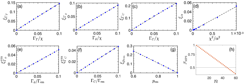
Figure 9: Scaling of the error rate $\xi$ in ${{\mathcal{F}}_{{\rm{\rm MPS}}}}$ for creating the cluster state [Eq. 7] using pulse sequence in Fig. 2 as a function of: the transmon decay during unitary operation (a), transmon dephasing during unitary operation (b), cavity decay during unitary operation (c), transmon anharmonicity during unitary operation (d), transmon dephasing during photon emission (e), cavity decay during photon emission (f), and the photon retrieval efficiency (g). The panel (h) show the MPDO calculation of ${{\mathcal{F}}_{{\rm{\rm MPS}}}}$ versus the cluster state photon number $n$, with transmon parameters in section D.2. The horizontal line denotes ${\cal F}_{\rm MPS}=1/2$.

And further trace out the environmental modes to get ${W_{\rm ph}}={\rm Tr}_{{{\varepsilon_{T}},{\varepsilon_{C}}}}[{{M_{\rm ph}}\otimes\bar{M}_{\rm ph}}]$. After that, we include the transmon dephasing by applying Eq. 37, to finish the construction of ${W_{\rm ph}}$.

Appendix D Additional scaling data for MPS preparation fidelity

D.1 Scaling of the error rate $\chi$

As shown in the main text, we can compute the scaling of the coefficient $\xi$ of the exponentially decaying fidelity ${\cal F}_{\rm MPS}=e^{-\xi\cdot n}$ with the slope (error rate) $\xi$ as a function of various imperfections. This scaling is numerically shown here in Fig. 9(a-g), where each data point is extracted from a MPDO calculation of the relation between ${\cal F}_{\rm MPS}$ and the photon number $n$ (an example is shown in Fig. 3a), with only the specific decoherence channel turned on. For example, in Fig. 9(a) only the transmon decay ${\Gamma_{T}}$ is turned on. From Fig. 9(a-g) we obtain all individual terms in Eq. 12, with non-universal coefficients in Eq. 16 for the cluster state generation with the pulse sequence in Fig. 2. In the regime where the error per photon generation is small, we can estimate the total error $\xi$ by simply adding these individual terms, thus obtaining Eq. 12.

D.2 Fidelity versus photon number for transmon parameters in Ref. Besse et al. (2020)

In Fig. 3(a) we showed the fidelity versus the cluster state photon number for the state-of-the-art experimental parameters shown in section II.4. To better compare it with the experimentally demonstrated result Besse et al. (2020), here we compute the same relation with the transmon properties reported there, while other parameters stays the same as that in section II.4. Specifically, we choose ${\Gamma_{T}}=$47.62\text{\,}\rm\mathrm{k}\mathrm{H}\mathrm{z}$$, ${\Gamma_{\phi}}=$58.82\text{\,}\rm\mathrm{k}\mathrm{H}\mathrm{z}$$, $\alpha=2\pi\times-$303\text{\,}\rm\mathrm{M}\mathrm{H}\mathrm{z}$$, and $\chi={\rm{2}}\pi\times-$5\text{\,}\rm\mathrm{M}\mathrm{H}\mathrm{z}$$ Besse et al. (2020). The result is shown in Fig. 9(h), from which we get $N_{\rm ph}\approx 47$.

D.3 Achievable entanglement length $N_{\rm ph}$ with MPS bond dimension $D$

The entanglement length ${N_{{\rm{ph}}}}=\log 2/\xi$ is determined by the error rate per photon $\xi$ [Eq. 12]. To produce an MPS with bond dimension $D$, we need to implement unitaries on $2D$-dimensional Hilbert space. As numerical evidence suggesting that Lee et al. (2018b) the time cost of implementing a general unitary in $N$-dimensional Hilbert space using the quantum optimal control approach scales as $O(N^{2})$, it takes $T^{D}_{\rm MPS}=O(D^{2})$ to implement above unitaries. This lead to increased decoherence as the coefficients ${\beta_{C}},{\beta_{T}},{\beta_{\phi}},{\beta_{\alpha}}$ in Eq. 8 are proportional to $T^{D}_{\rm MPS}$. In the regime of ${p_{{\rm{em}}}}\approx 1$ and $\beta_{0}\approx 0$ (typical for current experimental platforms Heeres et al. (2017); Besse et al. (2020)), one can thus estimate the scaling of $\xi$ as

$${\xi}\approx T_{{\rm{MPS}}}^{D}{\xi_{{\rm{unit}}}}+\xi_{{\rm{em}}}^{{\rm{src}}}+\xi_{{\rm{em}}}^{{\rm{ph}}}\sim O({{D^{2}}}).$$ (40)

Thus the dominant part lead to a qualitative scaling of ${N_{{\rm{ph}}}}\sim{D^{-2}}$.

Appendix E Isometric tensor network states

In this section, we provide more details on the definition of isometric tensor network states (isoTNS) Zaletel and Pollmann (2020).

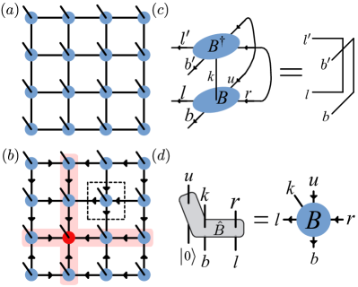
Figure 10: The projected entangled pair states (PEPS) and isometric tensor network states (isoTNS). (a) PEPS are states represented by a network of tensors, where the tensor at each site is of physical dimension $d$, and is connected to that of the neighboring sites with virtual bonds of dimension $D$. (b) IsoTNS are a subclass of PEPS, where the tensors satisfy isometry conditions denoted by the arrows. The red (gray) shaded lines denote the orthogonality hypersurface of isoTNS, and their crossing point [the red (dark gray) dot] denote the orthogonality center of isoTNS. (c) The isometry condition for the tensor inside the dashed box in panel (b). Here the incoming virtual legs and the physical legs of the tensor are contracted with the corresponding legs of the complex conjugate of the tensor, yield identity on the outgoing legs. This is also mathematically shown in Eq. 42. (d) One can map a three-qubit ‘L’-shaped quantum gate (see Fig. 8) to an isoTNS tensor of bond dimension $D=d$.

To start, first we recall the definition of the projected entangled pair states (PEPS) Verstraete and Cirac , which are defined through a network of tensors that are connected with each other, with one tensor at each lattice site (see Fig. 10a). The wavefunction of PEPS is obtained by contracting the connected (virtual) legs of the tensors, as

$$\left|\Psi_{\mathrm{PEPS}}\right\rangle=\sum_{\{k\}=0}^{d-1}\mathcal{F}_{2\mathrm{D}}(\{B_{[i,j]_{lurb}}^{k}\})|\{k\}\rangle,$$ (41)

where the ${B_{\left[{i,j}\right]lurd}^{k}}$ is a rank-5 tensor on the site $(i,j)$, which has virtual indices $l.u,r,b$ of bond dimension $D$ and physical index $k$ of physical dimension $d$. And the symbol ${\cal F}_{2D}$ denote the contraction of the connected virtual indices. PEPS serve as a natural extension of MPS in higher dimensions, and has wide applications in describing higher-dimensional many body systems Orús (2014, 2019); Cirac et al. (2020).

IsoTNS is a subclass of PEPS, where the tensors satisfy certain isometry conditions. The isometry condition means that, when the incoming legs (denoted by the arrows in Fig. 10b) and the physical legs of a tensor are contracted with corresponding legs of the complex conjugate of this tensor, the remaining legs yield an identity. For example, the tensor in the dashed box in Fig. 10(b) obeys

$$\sum\limits_{k,ur}{{B_{[{i,j}]}^{k}}_{lurb}{{({{B_{[{i,j}]}^{k}}_{l^{\prime}urb^{\prime}}})}^{*}}}={\delta_{bb^{\prime}}}{\delta_{ll^{\prime}}},$$ (42)

which is shown graphically in Fig. 10(c). Moreover, the two red shaded lines in Fig. 10(b) only have incoming arrows, which are termed the orthogonality hypersurface of isoTNS, and their intersection is the orthogonality center of the isoTNS Zaletel and Pollmann (2020).

As shown in Ref. Wei et al. , one can convert an isoTNS tensor $B_{\left[{i,j}\right]lurb}^{k}$ of the bond dimension $D$ into a ‘L’-shaped unitary of the form

$${\hat{B}_{[{i,j}]}}=\sum\limits_{lurb,k}{{B_{[{i,j}]}^{k}}_{lurb}}{|{u,k,r}\rangle}\langle{0,b,l}|,$$ (43)

where the indices are identified in Fig. 10(d) for the case of bond dimension $D=d$. Here the rank-5 tensor ${{B_{[{i,j}]}^{k}}_{lurb}}$ also satisfy the same isometry condition Eq. 42. This show that the gates in the photon generation scheme shown in Fig. 8 can be identified as isoTNS tensors. Increasing isoTNS bond dimension corresponds to increasing the arm length of the ‘L’-shaped unitary.

In this way, one can generate isoTNS by sequentially applying overlapping ‘L’-shape unitaries, which lead to the photonic isoTNS generation protocol discussed in section III.3.3. This fact further implies that isoTNS is a subclass of rp-PEPS Wei et al. since we can cover the ‘L’-shape unitaries by plaquette unitaries.

E.1 IsoTNS representation of the toric code

In general, the ${\mathbb{Z}}_{\lambda}$ toric code can be written as an isoTNS with the translational-invariant tensor at each site as Schuch et al. (2010)

$$B_{lurd}^{{i_{1}}{i_{2}}{i_{3}}{i_{4}}}=\frac{1}{\lambda}\delta_{l-u}^{{i_{1}}}\delta_{u-r}^{{i_{2}}}\delta_{r-b}^{{i_{3}}}\delta_{b-l}^{{i_{4}}},$$ (44)

where

$$\delta_{b}^{a}=\left\{\begin{array}[]{l}1,\qquad a=b\,\,\bmod\,\,\lambda\\ 0,\qquad{\rm{otherwise.}}\end{array}\right.$$ (45)

This is a tensor of bond dimension $\lambda$ and physical dimension $\lambda^{4}$, and satisfies the isometry condition Eq. 42.

Appendix F Control universality of $H_{\rm{array}}(t)$

Here we show the Hamiltonian $H_{\rm{array}}(t)$ [Eq. 19] can universally control the Hilbert space ${{\cal H}^{L_{C}\times m}_{\rm array}}={({{{\cal H}_{\rm src}}})^{\otimes L_{C}\times m}}$. Let us consider case of two cQED sequential photon sources coupled to each other ($L_{C}=1$ and $m=2$), that the whole Hilbert space is

$${{\cal H}^{1\times 2}_{\rm array}}={{\cal H}_{T}}\otimes{{\cal H}_{C}}\otimes{{\cal H}_{C}}\otimes{{\cal H}_{T}}.$$ (46)

We know the Hamiltonian for each sequential photon source can control one ${{{\cal H}_{\rm src}}}$ universally. This means one can create arbitrary Hamiltonians that act on each Hilbert space ${{\cal H}_{C}}$ of the cavity mode (see Eq. 47 below). Together with the bilinear interaction $H_{\rm int}^{ij}$ [Eq. 18] between two cavities, one can apply an analogous argument in Ref. Lloyd and Braunstein (1999), that by arithmetic operation and taking commutators between the bilinear coupling $H_{\rm int}^{12}$ [cf. Eq. 18] and single cavity Hamiltonians

$${H_{1}}={\rm poly}({{a_{1}},a_{1}^{\dagger}}),\quad{H_{2}}={\rm poly}({{a_{2}},a_{2}^{\dagger}}),$$ (47)

we can generate arbitrary polynomial form of Hamiltonian

$${H_{12}}={\rm poly}({{a_{1}},a_{1}^{\dagger},{a_{2}},a_{2}^{\dagger}})\in{{\cal H}_{C}}\otimes{{\cal H}_{C}}.$$ (48)

This immediately implies that we can universally control the Hilbert space of two cavities Lloyd and Braunstein (1999). Together with universal control on each sequential photon source, we can use Lemma 5.5 of Ref. Hofmann and Keyl to combine the universality of two ${{\cal H}_{\rm src}}$ and ${{\cal H}_{C}}\otimes{{\cal H}_{C}}$ to the whole ${{\cal H}^{1\times 2}_{\rm array}}$, which shows that we can universally control ${{\cal H}^{1\times 2}_{\rm array}}$ with $H_{\rm{array}}(t)$ (here $L_{C}=1$ and $m=2$). By repeatedly applying Lemma 5.5 of Ref. Hofmann and Keyl , one can show $H_{\rm{array}}(t)$ is further able to control ${{\cal H}^{L_{C}\times m}_{\rm array}}$.

References

- O’Brien et al. (2009) J. L. O’Brien, A. Furusawa, and J. Vučković, Nature Photonics 3, 687 (2009).
- Gisin and Thew (2007) N. Gisin and R. Thew, Nature photonics 1, 165 (2007).
- Kimble (2008) H. J. Kimble, Nature 453, 1023 (2008).
- Degen et al. (2017) C. L. Degen, F. Reinhard, and P. Cappellaro, Reviews of Modern Physics 89, 1 (2017).
- Burnham and Weinberg (1970) D. C. Burnham and D. L. Weinberg, Physical Review Letters 25, 84 (1970).
- Zhong et al. (2018) H. S. Zhong, Y. Li, W. Li, L. C. Peng, Z. E. Su, Y. Hu, Y. M. He, X. Ding, W. Zhang, H. Li, L. Zhang, Z. Wang, L. You, X. L. Wang, X. Jiang, L. Li, Y. A. Chen, N. L. Liu, C. Y. Lu, and J. W. Pan, Physical Review Letters 121, 1 (2018).
- Gheri et al. (1998) K. M. Gheri, C. Saavedra, P. Törmä, J. I. Cirac, and P. Zoller, Physical Review A 58, R2627 (1998).
- Saavedra et al. (2000) C. Saavedra, K. M. Gheri, P. Törmä, J. I. Cirac, and P. Zoller, Physical Review A 61, 62311 (2000).
- Schön et al. (2005) C. Schön, E. Solano, F. Verstraete, J. I. Cirac, and M. M. Wolf, Physical Review Letters 95, 1 (2005).
- Schön et al. (2007) C. Schön, K. Hammerer, M. M. Wolf, J. I. Cirac, and E. Solano, Physical Review A 75, 1 (2007).
- Lindner and Rudolph (2009) N. H. Lindner and T. Rudolph, Physical Review Letters 103, 1 (2009).
- (12) K. Tiurev, M. H. Appel, P. L. Mirambell, M. B. Lauritzen, A. Tiranov, P. Lodahl, and A. S. Sørensen, arXiv:2007.09295 .
- Wei et al. (2021) Z.-Y. Wei, D. Malz, A. González-Tudela, and J. I. Cirac, Phys. Rev. Research 3, 23021 (2021).
- (14) D. Perez-Garcia, F. Verstraete, M. M. Wolf, and J. I. Cirac, arXiv:0608197 [quant-ph] .
- Schollwöck (2011) U. Schollwöck, Annals of Physics 326, 96 (2011).
- Orús (2014) R. Orús, Annals of Physics 349, 117 (2014).
- Cirac et al. (2020) J. I. Cirac, D. Perez-Garcia, N. Schuch, and F. Verstraete, “Matrix product states and projected entangled pair states: Concepts, symmetries, and theorems,” (2020), arXiv:2011.12127 .
- Schwartz et al. (2016) I. Schwartz, D. Cogan, E. R. Schmidgall, Y. Don, L. Gantz, O. Kenneth, N. H. Lindner, and D. Gershoni, Science 354, 434 (2016).
- Eichler et al. (2015) C. Eichler, J. Mlynek, J. Butscher, P. Kurpiers, K. Hammerer, T. J. Osborne, and A. Wallraff, Physical Review X 5, 1 (2015).
- Besse et al. (2020) J.-C. Besse, K. Reuer, M. C. Collodo, A. Wulff, L. Wernli, A. Copetudo, D. Malz, P. Magnard, A. Akin, M. Gabureac, G. J. Norris, J. I. Cirac, A. Wallraff, and C. Eichler, Nature Communications 11, 1 (2020).
- Economou et al. (2010) S. E. Economou, N. Lindner, and T. Rudolph, Physical Review Letters 105, 1 (2010).
- Gimeno-Segovia et al. (2019) M. Gimeno-Segovia, T. Rudolph, and S. E. Economou, Physical Review Letters 123, 70501 (2019).
- Russo et al. (2019) A. Russo, E. Barnes, and S. E. Economou, New Journal of Physics 21, 55002 (2019).
- Bekenstein et al. (2020) R. Bekenstein, I. Pikovski, H. Pichler, E. Shahmoon, S. F. Yelin, and M. D. Lukin, Nature Physics 16, 676 (2020).
- (25) S. Bartolucci, P. Birchall, H. Bombin, H. Cable, C. Dawson, M. Gimeno-Segovia, E. Johnston, K. Kieling, N. Nickerson, M. Pant, F. Pastawski, T. Rudolph, and C. Sparrow, arXiv:2101.09310 .
- Pichler et al. (2017) H. Pichler, S. Choi, P. Zoller, and M. D. Lukin, Proceedings of the National Academy of Sciences 114, 11362 (2017).
- Dhand et al. (2018) I. Dhand, M. Engelkemeier, L. Sansoni, S. Barkhofen, C. Silberhorn, and M. B. Plenio, Physical Review Letters 120 (2018).
- Xu and Fan (2018) S. Xu and S. Fan, APL Photonics 3 (2018), 10.1063/1.5044248.
- (29) K. Wan, S. Choi, I. H. Kim, N. Shutty, and P. Hayden, “Fault-tolerant qubit from a constant number of components,” arXiv:2011.08213 .
- Zhan and Sun (2020) Y. Zhan and S. Sun, Physical Review Letters 125, 223601 (2020).
- (31) Y. Shi and E. Waks, arXiv:2101.07772 .
- (32) H. Bombin, I. H. Kim, D. Litinski, N. Nickerson, M. Pant, F. Pastawski, S. Roberts, and T. Rudolph, arXiv:2103.08612 .
- (33) F. Verstraete and J. I. Cirac, arXiv:0407066 [cond-mat] .
- Verstraete et al. (2006) F. Verstraete, M. M. Wolf, D. Perez-Garcia, and J. I. Cirac, Physical Review Letters 96, 1 (2006).
- Schuch et al. (2007) N. Schuch, M. M. Wolf, F. Verstraete, and J. I. Cirac, Physical Review Letters 98, 1 (2007).
- (36) Z.-Y. Wei, D. Malz, and J. I. Cirac, “Sequential generation of projected entangled-pair states,” arXiv:2107.05873 [quant-ph] .
- Zaletel and Pollmann (2020) M. P. Zaletel and F. Pollmann, Physical Review Letters 124, 37201 (2020).
- Hein et al. (2004) M. Hein, J. Eisert, and H. J. Briegel, Physical Review A 69, 62311 (2004).
- Schuch et al. (2010) N. Schuch, I. Cirac, and D. Pérez-García, Annals of Physics 325, 2153 (2010).
- Levin and Wen (2005) M. A. Levin and X. G. Wen, Physical Review B 71, 1 (2005).
- Gu et al. (2009) Z.-C. Gu, M. Levin, B. Swingle, and X.-G. Wen, Physical Review B 79, 85118 (2009).
- Buerschaper et al. (2009) O. Buerschaper, M. Aguado, and G. Vidal, Physical Review B 79, 085119 (2009).
- Soejima et al. (2020) T. Soejima, K. Siva, N. Bultinck, S. Chatterjee, F. Pollmann, and M. P. Zaletel, Physical Review B 101, 1 (2020).
- Note (1) Note that the string-net states are originally defined on the hexagonal lattice Levin and Wen (2005). Since one can embed a hexagonal lattice into a square lattice, one can create string-net states using the schemes we show in this paper, which are based on square lattices.
- Takeuchi et al. (2019) Y. Takeuchi, T. Morimae, and M. Hayashi, Scientific Reports 9, 1 (2019).
- Asavanant et al. (2019) W. Asavanant, Y. Shiozawa, S. Yokoyama, B. Charoensombutamon, H. Emura, R. N. Alexander, S. Takeda, J. I. Yoshikawa, N. C. Menicucci, H. Yonezawa, and A. Furusawa, Science (New York, N.Y.) 366, 373 (2019).
- J. et al. (2021) S. K. J., L. Y.-J, S. A., K. C., N. M., J. C., C. Z., Q. C., M. X., D. A., G. C., A. I., A. F., A. K., A. J., B. R., B. J. C., B. R., B. J., B. A., B. A., B. M., B. B. B., B. D. A., B. B., B. N., C. B., C. R., C. W., D. S., D. A. R., E. D., E. C., F. L., F. E., F. A. G., F. B., G. M., G. A., G. J. A., H. M. P., H. S. D., H. J., H. S., H. T., H. W. J., I. L. B., I. S. V., J. E., J. Z., K. D., K. K., K. T., K. S., K. P. V., K. A. N., K. F., L. D., L. P., L. A., L. E., M. O., M. J. R., M. M., M. K. C., M. M., M. S., M. W., M. J., N. O., N. M., N. C., N. M. Y., O. T. E., O. A., P. B., P. A., R. N. C., S. D., S. V., S. D., S. M., V. B., W. T. C., Y. Z., Y. P., Y. J., Z. A., N. H., B. S., M. A., C. Y., K. J., S. V., K. A., K. M., P. F., and R. P., Science 374, 1237 (2021).
- Semeghini et al. (2021) G. Semeghini, H. Levine, A. Keesling, S. Ebadi, T. T. Wang, D. Bluvstein, R. Verresen, H. Pichler, M. Kalinowski, R. Samajdar, A. Omran, S. Sachdev, A. Vishwanath, M. Greiner, V. Vuletic, and M. D. Lukin, “Probing Topological Spin Liquids on a Programmable Quantum Simulator,” (2021), arXiv:2104.04119 [quant-ph] .
- Jarzyna and Demkowicz-Dobrzański (2013) M. Jarzyna and R. Demkowicz-Dobrzański, Physical Review Letters 110, 1 (2013).
- Chabuda et al. (2020) K. Chabuda, J. Dziarmaga, T. J. Osborne, and R. Demkowicz-Dobrzański, Nature Communications 11, 1 (2020).
- Miguel-Ramiro et al. (2021) J. Miguel-Ramiro, A. Pirker, and W. Dür, npj Quantum Information 7, 1 (2021).
- Huang (a) Y. Huang, (a), arXiv:1505.00772 .
- Dalzell and Brandão (2019) A. M. Dalzell and F. G. Brandão, Quantum 3 (2019), 10.22331/q-2019-09-23-187.
- Huang (b) Y. Huang, (b), arXiv:1903.10048 .
- (55) N. Schuch and F. Verstraete, arXiv:1711.06559 .
- Koczor et al. (2020) B. Koczor, S. Endo, T. Jones, Y. Matsuzaki, and S. C. Benjamin, New Journal of Physics 22 (2020), 10.1088/1367-2630/ab965e.
- Azuma et al. (2015) K. Azuma, K. Tamaki, and H. K. Lo, Nature Communications 6 (2015), 10.1038/ncomms7787.
- Axline et al. (2018) C. J. Axline, L. D. Burkhart, W. Pfaff, M. Zhang, K. Chou, P. Campagne-Ibarcq, P. Reinhold, L. Frunzio, S. M. Girvin, L. Jiang, M. H. Devoret, and R. J. Schoelkopf, Nature Physics 14, 705 (2018).
- Kurpiers et al. (2018) P. Kurpiers, P. Magnard, T. Walter, B. Royer, M. Pechal, J. Heinsoo, Y. Salathé, A. Akin, S. Storz, J. C. Besse, S. Gasparinetti, A. Blais, and A. Wallraff, Nature 558, 264 (2018).
- Magnard et al. (2020) P. Magnard, S. Storz, P. Kurpiers, J. Schär, F. Marxer, J. Lütolf, T. Walter, J.-C. Besse, M. Gabureac, K. Reuer, and Others, Physical Review Letters 125, 260502 (2020).
- Reagor et al. (2016) M. Reagor, W. Pfaff, C. Axline, R. W. Heeres, N. Ofek, K. Sliwa, E. Holland, C. Wang, J. Blumoff, K. Chou, M. J. Hatridge, L. Frunzio, M. H. Devoret, L. Jiang, and R. J. Schoelkopf, Physical Review B 94, 1 (2016).
- Note (2) Here we neglected the higher order Hamiltonian terms such as the Kerr non-linearity Heeres et al. (2017). In principle, one can also include these terms in the pulse optimization.
- Strauch (2012) F. W. Strauch, Physical Review Letters 109, 1 (2012).
- Krastanov et al. (2015) S. Krastanov, V. V. Albert, C. Shen, C. L. Zou, R. W. Heeres, B. Vlastakis, R. J. Schoelkopf, and L. Jiang, Physical Review A 92 (2015).
- Machnes et al. (2018) S. Machnes, E. Assémat, D. Tannor, and F. K. Wilhelm, Physical Review Letters 120 (2018).
- Briegel and Raussendorf (2001) H. J. Briegel and R. Raussendorf, Physical Review Letters 86, 910 (2001).
- Heeres et al. (2017) R. W. Heeres, P. Reinhold, N. Ofek, L. Frunzio, L. Jiang, M. H. Devoret, and R. J. Schoelkopf, Nature Communications 8 (2017).
- Note (3) Note that the thermal excitations (photon gain) in the cavity and the transmon are neglected here.
- Chou et al. (2018) K. S. Chou, J. Z. Blumoff, C. S. Wang, P. C. Reinhold, C. J. Axline, Y. Y. Gao, L. Frunzio, M. H. Devoret, L. Jiang, and R. J. Schoelkopf, Nature 561, 368 (2018).
- Note (4) The photon retrieval efficiency depends on the explicit realization of the on-demand photon emission process, which we do not specify in this work. For example, in Ref. Besse et al. (2020) the system is modeled with .
- Rebentrost and Wilhelm (2009) P. Rebentrost and F. K. Wilhelm, Physical Review B 79, 2 (2009).
- Note (5) Here we assume that the realization of our protocol using cavity + transmon system can also be modeled with the photon retrieval efficiency , same as that in Ref. Besse et al. (2020).
- Note (6) Since the emitter is always in its ground state at the start of each unitary operation (i.e. after each photon emission), the transmon will only transiently populated during each unitary operation.
- Lee et al. (2018a) J. Lee, C. Arenz, H. Rabitz, and B. Russell, New Journal of Physics 20 (2018a), 10.1088/1367-2630/aac6f3.
- Note (7) Here we do not include the transmons in the ancilla space due to their relatively short coherence time compared to the photons in the cavities. However, in principle, one can include the transmons into the ancilla as well to further increase its Hilbert space dimension.
- Wang et al. (2016) C. Wang, Y. Y. Gao, P. Reinhold, R. W. Heeres, N. Ofek, K. Chou, C. Axline, M. Reagor, J. Blumoff, K. M. Sliwa, L. Frunzio, S. M. Girvin, L. Jiang, M. Mirrahimi, M. H. Devoret, and R. J. Schoelkopf, Science 352, 1087 (2016).
- Gao et al. (2018) Y. Y. Gao, B. J. Lester, Y. Zhang, C. Wang, S. Rosenblum, L. Frunzio, L. Jiang, S. M. Girvin, and R. J. Schoelkopf, Physical Review X 8, 21073 (2018).
- Note (8) The source point of rp-PEPS is precisely defined as the location of the first plaquette unitary Wei et al. .
- Huggins et al. (2019) W. Huggins, P. Patil, B. Mitchell, K. Birgitta Whaley, and E. Miles Stoudenmire, Quantum Science and Technology 4 (2019), 10.1088/2058-9565/aaea94.
- Liu et al. (2019) J.-G. Liu, Y.-H. Zhang, Y. Wan, and L. Wang, Physical Review Research 1, 23025 (2019).
- Rosenblum et al. (2018) S. Rosenblum, Y. Y. Gao, P. Reinhold, C. Wang, C. J. Axline, L. Frunzio, S. M. Girvin, L. Jiang, M. Mirrahimi, M. H. Devoret, and R. J. Schoelkopf, Nature Communications 9 (2018), 10.1038/s41467-018-03059-5.
- Dennis et al. (2002) E. Dennis, A. Kitaev, A. Landahl, and J. Preskill, Journal of Mathematical Physics 43, 4452 (2002).
- Kitaev (2003) A. Y. Kitaev, Annals of Physics 303, 2 (2003).
- (84) Y.-J. Liu, K. Shtengel, A. Smith, and F. Pollmann, arXiv:2110.02020 .
- Bullock and Brennen (2007) S. S. Bullock and G. K. Brennen, Journal of Physics A: Mathematical and Theoretical 40, 3481 (2007).
- Duclos-Cianci and Poulin (2013) G. Duclos-Cianci and D. Poulin, Physical Review A 87, 1 (2013).
- Watson et al. (2015) F. H. E. Watson, H. Anwar, and D. E. Browne, Physical Review A 92, 1 (2015).
- Zhang et al. (2019) Y. Zhang, B. J. Lester, Y. Y. Gao, L. Jiang, R. J. Schoelkopf, and S. M. Girvin, Physical Review A 99, 1 (2019).
- Ofek et al. (2016) N. Ofek, A. Petrenko, R. Heeres, P. Reinhold, Z. Leghtas, B. Vlastakis, Y. Liu, L. Frunzio, S. M. Girvin, L. Jiang, M. Mirrahimi, M. H. Devoret, and R. J. Schoelkopf, Nature 536, 441 (2016).
- Campagne-Ibarcq et al. (2020) P. Campagne-Ibarcq, A. Eickbusch, S. Touzard, E. Zalys-Geller, N. E. Frattini, V. V. Sivak, P. Reinhold, S. Puri, S. Shankar, R. J. Schoelkopf, L. Frunzio, M. Mirrahimi, and M. H. Devoret, Nature 584, 368 (2020).
- Ma et al. (2019) W.-L. Ma, M. Zhang, Y. Wong, K. Noh, S. Rosenblum, P. Reinhold, R. J. Schoelkopf, and L. Jiang, Physical Review Letters 125, 110503 (2019).
- Schulte-Herbrüggen et al. (2011) T. Schulte-Herbrüggen, A. Spörl, N. Khaneja, and S. J. Glaser, Journal of Physics B: Atomic, Molecular and Optical Physics 44 (2011).
- Abdelhafez et al. (2019) M. Abdelhafez, D. I. Schuster, and J. Koch, Physical Review A 99, 52327 (2019).
- Plenio and Knight (1998) M. B. Plenio and P. L. Knight, Reviews of Modern Physics 70, 101 (1998).
- Lee et al. (2018b) J. Lee, C. Arenz, H. Rabitz, and B. Russell, New Journal of Physics 20, 1 (2018b).
- Orús (2019) R. Orús, Nature Reviews Physics 1, 538 (2019).
- Lloyd and Braunstein (1999) S. Lloyd and S. L. Braunstein, Physical Review Letters 82, 1784 (1999).
- (98) T. Hofmann and M. Keyl, arXiv:1712.07613 .