Dynamic Attentive Graph Learning for Image Restoration

Abstract

Non-local self-similarity in natural images has been verified to be an effective prior for image restoration. However, most existing deep non-local methods assign a fixed number of neighbors for each query item, neglecting the dynamics of non-local correlations. Moreover, the non-local correlations are usually based on pixels, prone to be biased due to image degradation. To rectify these weaknesses, in this paper, we propose a dynamic attentive graph learning model (DAGL) to explore the dynamic non-local property on patch level for image restoration. Specifically, we propose an improved graph model to perform patch-wise graph convolution with a dynamic and adaptive number of neighbors for each node. In this way, image content can adaptively balance over-smooth and over-sharp artifacts through the number of its connected neighbors, and the patch-wise non-local correlations can enhance the message passing process. Experimental results on various image restoration tasks: synthetic image denoising, real image denoising, image demosaicing, and compression artifact reduction show that our DAGL can produce state-of-the-art results with superior accuracy and visual quality. The source code is available at https://github.com/jianzhangcs/DAGL.

1 Introduction

Image restoration (IR) is typically an ill-posed inverse problem aiming to restore a high-quality image ($\mathbf{I}_{HQ}$) from its degraded measurement ($\mathbf{I}_{LQ}$) corrupted by various degradation factors. The degradation process can be defined as $\mathbf{I}_{LQ}=\mathbf{H}\mathbf{I}_{HQ}+\mathbf{n}$, where $\mathbf{H}$ is a linear degradation matrix, and $\mathbf{n}$ represents additive noise [48, 55]. According to $\mathbf{H}$, IR can be categorized into many subtasks, e.g., denoising, compression artifact reduction, demosaicing, super-resolution, compressive sensing [49, 53, 54, 46].

The rise of deep learning has greatly facilitated the development of image restoration. Many deep learning-based methods [49, 50, 51, 33] have been proposed to solve this ill-posed problem. Despite the remarkable success, most methods focus on learning from a lot of external training data without fully utilizing the internal prior in images. By contrast, many classic model-based methods are implemented based on various priors, e.g., total variation [26], sparse representation [9, 10, 47], and self-similarity [4, 7]. The self-similarity assumes that similar content would recur across the whole image, and the local content can be recovered with the help of similar items from other places. Inspired by [4], non-local neural networks [40] utilized self-similarity via deep networks, which are subsequently introduced to many image restoration tasks [20, 52]. However, these pixel-wise non-local methods are easily influenced by noisy signals within corrupted images. [18, 19] were proposed to establish long-range correlations on patch level. Nevertheless, the patch matching step is isolated from the training process. In N3Net [29], a differentiable $K$-Nearest Neighbor (KNN) method was proposed. However, restricted by the high complexity of channel-wise feature fusion, N3Net can only perform the non-local operation within a small search region ($10\times 10$) and a small number of matching patches. Some very recent methods [24, 23, 5] proposed more efficient patch-wise non-local methods. But they followed the same paradigm as existing non-local methods to construct fully connected correlations.

In general, the repeatability of different image content is distinct, causing different requirements of non-local correlations in restoring different image content. An early work [56] has well studied this property, finding that smooth image contents recur much more frequently than complex image details, and they should be treated differently.

Graph convolutional network (GCN) is a special non-local method designed to process the graph data by establishing long-range correlations in non-Euclidean space. However, the large domain gap limits the application of this flexible non-local method in computer vision community. Recently, few works [36, 35, 21] proposed to apply GCN to image restoration tasks. Specifically, [36] and [35] are built based on Edge-Conditioned Convolution (ECC) [32] for image denoising. However, they constructed the long-range correlations based on pixels and assigned a fixed number of neighbors for each graph node. In [21], a patch-wise GCN method is proposed for facial expression restoration. Nevertheless, the adjacency matrix is predefined based on the facial structure and isolated from the training process. In addition to ECC, graph attention network (GAT) [38] is a popular graph model combined with attention mechanism to identify the importance of different neighboring nodes.

Inspired by GAT, in this paper, we propose a novel dynamic attentive graph learning model (DAGL) for image restoration. In our proposed DAGL, the corrupted image is recovered in an image-specific and adaptive graph constructed based on local feature patches.

2 Related Works

Our model is closely related to image restoration algorithms, non-local attention methods, and graph convolutional networks. Since in what follows, we give a brief review of these aspects and some most relevant methods.

2.1 Image Restoration Architectures

Driven by the success of deep learning, almost all recent top-performing image restoration methods are implemented based on deep networks. Stacking convolutional layers is the most well-known CNN-based strategy. Dong et al. proposed ARCNN [8] for image restoration with several stacked convolutional layers. Subsequently, [49, 51, 50] utilized deeper convolutional architecture and residual learning to further enhance image restoration performance. Recently, abundant novel models and function units were proposed. MemNet [33] utilized the dense connection in convolutional layers for image denoising. To enlarge the receptive field, hourglass-shaped architecture [14, 43, 3, 44, 17, 30], dilated convolution [50, 39], and very deep residual networks [53, 52] are often used. However, most methods are plain networks and neglect to use non-local information.

2.2 Non-local Prior for Image Restoration

Non-local self-similarity is an effective prior that has been widely used in image restoration tasks. Some classic methods [7, 4] utilized self-similarity for image denoising and achieved attractive performance. Following the importance of self-similarity, some recent approaches [52, 20] utilized this prior based on non-local neural networks [40]. Moreover, some patch-wise non-local methods [18, 19, 29] or transformer-based methods [5, 24] were proposed. These methods performed matching and aggregation in a non-local manner can be generally defined as:

$$\hat{\mathbf{x}}_{i}=\frac{1}{z_{i}}\sum_{{j}\in\mathbb{Q}}\phi(\mathbf{y}_{i},\mathbf{y}_{j})G(\mathbf{y}_{j}),\forall i,$$ (1)

where $\mathbb{Q}$ refers to the search region, and $z_{i}$ represents the normalizing constant calculated by $z_{i}=\sum_{{j}\in\mathbb{Q}}\phi(\mathbf{y}_{i},\mathbf{y}_{j})$. The function $\phi$ computes pair-wise affinity between query item $\mathbf{y}_{i}$ and key item $\mathbf{y}_{j}$. $G$ is a feature transformation function that generates a new representation of $\mathbf{y}_{j}$. While the above operation aggregates adequate information for the query item, the feature aggregation is restricted to be fully connected, involving all features within the search region, no matter how similar they are to the query item.

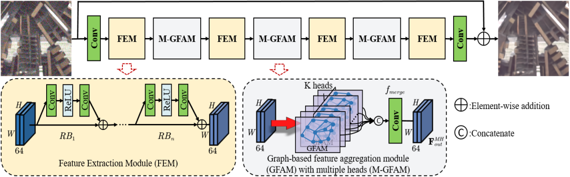
Figure 1: Proposed dynamic attentive graph learning model (DAGL). The feature extraction module (FEM) employs residual blocks to extract deep features. The graph-based feature aggregation module (GFAM) constructs a graph with dynamic connections and performs patch-wise graph convolution. GFAM with multiple-heads (M-GFAM) jointly aggregates information from different representation subspaces.

2.3 Graph Convolutional Networks (GCN)

By extending convolutional neural networks (CNN) from grid data, such as images and videos, to graph-structured data, GCN has been attracting growing attention from the computer vision community due to its robust capacity of non-local feature aggregation. Not that without loss of generality, the commonly used non-local neural networks [40] can be viewed as a fully connected graph [12]. Recently, [21] utilized the predefined adjacency matrix to perform graph convolution for facial expression restoration. [36, 35] applied Edge-Conditioned Convolution (ECC) [32], a well-known GCN method, to image denoising task. [27] further extended ECC to 3D denoising tasks. Let us consider a graph that contains $N$ nodes: $\mathcal{G=(V,E)}$, where $\mathcal{V}$ is the set of graph nodes, and $\mathcal{E}$ is the set of edges. Let $\mathbf{v}_{i}\in\mathbb{R}^{l_{1}}$ denote a graph node and $\mathbf{e}_{ij}=(\mathbf{v}_{i},\mathbf{v}_{j})\in\mathcal{E}$ denote an edge pointing from $\mathbf{v}_{j}$ to $\mathbf{v}_{i}$. In ECC, there exists a shared filter-generating network $\mathcal{F}$: $\mathbb{R}^{s}\mapsto\mathbb{R}^{l_{2}\times l_{1}}$. Given an edge label $\mathbf{e}_{ij}\in\mathbb{R}^{s}$, it outputs an edge-specific embedding matrix $\mathbf{\Theta}_{ij}\in\mathbb{R}^{l_{2}\times l_{1}}$. The aggregation process of ECC is an averaging operation embedded by the edge-specific embedding matrix, which can be formalized as:

$$\hat{\mathbf{v}}_{i}=\frac{1}{|\mathcal{N}_{i}|}\sum_{j\in\mathcal{N}_{i}}\mathcal{F}(\mathbf{e}_{ij})\mathbf{v}_{j}+\mathbf{b}=\frac{1}{|\mathcal{N}_{i}|}\sum_{j\in\mathcal{N}_{i}}\mathbf{\Theta}_{ij}\mathbf{v}_{j}+\mathbf{b},$$ (2)

where $\mathcal{N}_{i}=\{j|(\mathbf{v}_{i},\mathbf{v}_{j})\in\mathcal{E}\}$ is the set of indexes of neighboring nodes of $\mathbf{v}_{i}$, and $\mathbf{b}\in\mathbb{R}^{l_{2}}$ is a learnable bias. Apart from ECC, graph attention network (GAT) [38] is also a popular GCN method, and our proposed DAGL is inspired by this method. Unlike ECC generating an embedding matrix through the edge label to perform embedding and averaging aggregation, GAT developed an attention weight for each edge based on the self-attention mechanism [37]. In this way, each node can aggregate the information selectively from all its connected neighbors. The calculation of the attention weight is defined as:

$$\alpha_{ij}=\frac{exp(LeakyReLU(\mathbf{a}^{T}[\mathbf{W}\mathbf{v}_{i}||\mathbf{W}\mathbf{v}_{j}]))}{\sum_{k\in\mathcal{N}_{i}}exp(LeakyReLU(\mathbf{a}^{T}[\mathbf{W}\mathbf{v}_{i}||\mathbf{W}\mathbf{v}_{k}]))},$$ (3)

where $\mathbf{W}\in\mathbb{R}^{l_{2}\times l_{1}}$ and $\mathbf{a}\in\mathbb{R}^{2l_{2}\times 1}$ refer to the learnable weight matrixes of shared linear transformations, and $||$ represents the concatenating operation. In the process of aggregation, the source node will be updated through the sum of all its connected neighbors weighted by the learnable attention weights:

$$\hat{\mathbf{v}}_{i}=\sum_{j\in\mathcal{N}_{i}}\alpha_{ij}\cdot\mathbf{W}\mathbf{v}_{j}.$$ (4)

Different from most GCN methods directly processing graph data, the main challenge of applying GCN to the image restoration community is how to construct a graph and perform graph convolution on regular grid data effectively. In this paper, we propose an improved graph attention model to perform patch-wise graph convolution with dynamic graph connections for image restoration. The proposed method achieves state-of-the-art performance on various image restoration tasks.

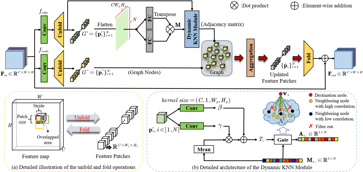
Figure 2: Detailed illustration of the proposed graph-based feature aggregation module (GFAM). The subfigure (a) elaborates the unfold and fold operations. The subfigure (b) presents the detailed architecture of the dynamic KNN module, which is used to generate a node-specific threshold to filter out graph connections with low importance.

3 Proposed Method

3.1 Framework

An overview of our proposed model (DAGL) is shown in Fig. 1, mainly composed of two components: feature extraction module (FEM) and graph-based feature aggregation module (GFAM) with multiple heads (M-GFAM). Similar to many image restoration networks, we add a global pathway from the input to the final output, which encourages the network to bypass low-frequency information. The feature extraction module comprises several residual blocks (RBs), and we follow the strategy in [52] to remove batch normalization [16] layers from residual blocks. The graph-based feature aggregation module is the core of our proposed DAGL, which is implemented based on graph attention networks (GAT) [38]. More details about GFAM will be given in the following subsection.

Our proposed model is optimized with the $\mathcal{L}2$ loss function. Given a training set $\{\mathbf{I}_{HQ}^{b},\mathbf{I}_{LQ}^{b}\}_{b=1}^{B}$, which contains $B$ training pairs. The goal of the training can be defined as:

$$\mathcal{L}(\theta)=\frac{1}{B}\sum_{b=1}^{B}\left\|\mathbf{I}_{HQ}^{b}-\mathcal{H}(\mathbf{I}_{LQ}^{b})\right\|^{2}_{2},$$ (5)

where $\mathcal{H}$ refers to the function of our proposed DAGL, and $\theta$ refers to the learnable parameters.

3.2 Graph-based Feature Aggregation Module

As mentioned previously, existing deep non-local methods and graph-based image restoration methods assigned a fixed number of neighbors for each query/node. The main difference is that deep non-local methods involve all items in the search region to update one query item, and the graph-based methods select $K$ nearest neighbors for each node. In this subsection, we will present our proposed graph-based feature aggregation module (GFAM), a dynamic solution to break this set pattern. Our GFAM constructs the long-range correlations based on 3D feature patches and assigns a dynamic number of neighbors for each query patch. The detailed illustration of our proposed GFAM is shown in Fig. 2, which is mainly composed of three phases: initialization, dynamic graph construction, and feature aggregation.

Initialization. In our GFAM, we first need to initialize some elements for constructing a graph $\mathcal{G}=(\mathcal{V},\mathcal{E})$ on regular grid data, where $\mathcal{V}$ is the set of nodes with $|\mathcal{V}|=N$ and $\mathcal{E}\subseteq\mathcal{V}\times\mathcal{V}$ is the set of edges. Assuming $N$ overlapped feature patches $\{\mathbf{p}_{i}\}_{i=1}^{N}$ with the patch size being $C\times W_{p}\times H_{p}$ ($C\times 7\times 7$ by default), neatly arranged in the input feature map $\mathbf{F}_{in}\in\mathbb{R}^{C\times W\times H}$. We apply two $1\times 1$ convolutional layers ($f_{edge}$ and $f_{node}$) to transform $\mathbf{F}_{in}$ to two independent representations and then utilize the unfold operation to extract the transformed feature patches into two groups: $G^{\prime}=\{\mathbf{p}_{i}^{\prime}\}_{i=1}^{N}$ and $G^{\prime\prime}=\{\mathbf{p}_{i}^{\prime\prime}\}_{i=1}^{N}$. The feature patches in $G^{\prime}$ and $G^{\prime\prime}$ have the following feature representations:

$$\begin{cases}&\mathbf{p}_{i}^{\prime}=f_{edge}(\mathbf{p}_{i})\\ &\mathbf{p}_{i}^{\prime\prime}=f_{node}(\mathbf{p}_{i}).\end{cases}$$ (6)

$G^{\prime}$ is used to build graph connections ($\mathcal{E}$), and $G^{\prime\prime}$ is assigned as the graph nodes.

Dynamic Graph Construction. The graph nodes in our method are directly assigned by feature patches in $G^{\prime\prime}$: $\mathcal{V}=G^{\prime\prime}$. In establishing graph connections, we select a dynamic number of neighbors for each node based on the nearest principle. For this purpose, we design a dynamic KNN module to generate an adaptive threshold for each node to select neighbors whose similarities are above the threshold. Specifically, given the set of feature patches $G^{\prime}$, we first flatten each feature patch into a feature vector. The pair-wise similarities can be efficiently calculated by dot product, producing a similarity matrix $\mathbf{M}\in\mathbb{R}^{N\times N}$. Let us consider $\mathbf{M}_{i,:}$, the $i$-th row of $\mathbf{M}$, representing similarities between the $i$-th node and the other nodes. The average of $\mathbf{M}_{i,:}$ is the fairly average importance of different nodes to the $i$-th node. Thus, it is an appropriate choice for the threshold, represented as $T_{i}$. As illustrated in Fig. 2(b), to improve the adaptability, we further apply a node-specific affine transformation to compute $T_{i}$:

$$T_{i}=\frac{\psi_{1}(\mathbf{p}_{i}^{\prime})}{N}\sum_{k=1}^{N}\mathbf{M}_{i,k}+\psi_{2}(\mathbf{p}_{i}^{\prime})=\frac{\gamma}{N}\sum_{k=1}^{N}\mathbf{M}_{i,k}+\beta,$$ (7)

where $\psi_{1}$ and $\psi_{2}$ are two independent convolutional layers with the kernel size being $C\times 1\times W_{p}\times H_{p}$ to embed each node to specific affine transformation parameters ($\beta$, $\gamma$). To achieve a differentiable threshold truncation, we utilize ReLU [25] function to truncate the negative part and keep the positive part. This process is formalized as:

$$\mathbf{A}_{i,:}=ReLU(\mathbf{M}_{i,:}-T_{i}),$$ (8)

where $\mathbf{A}\in\mathbb{R}^{N\times N}$ is the adjacency matrix in which $\mathbf{A}_{ij}$ is assigned the similarity weight if $\mathbf{p}_{j}^{\prime}$ connects to $\mathbf{p}_{i}^{\prime}$, otherwise equal to zero. Next, following the definition in Eq. 3, we normalize the similarity of all connected nodes (non-zero values in $\mathbf{A}_{i,:}$) by the softmax function to calculate the attention weights:

$$\alpha_{ij}=\frac{exp(\mathbf{A}_{ij})}{\sum_{k\in\mathcal{N}_{i}}exp(\mathbf{A}_{ik})},j\in\mathcal{N}_{i}.$$ (9)

Query patch in high-quality label

Similarity matrix

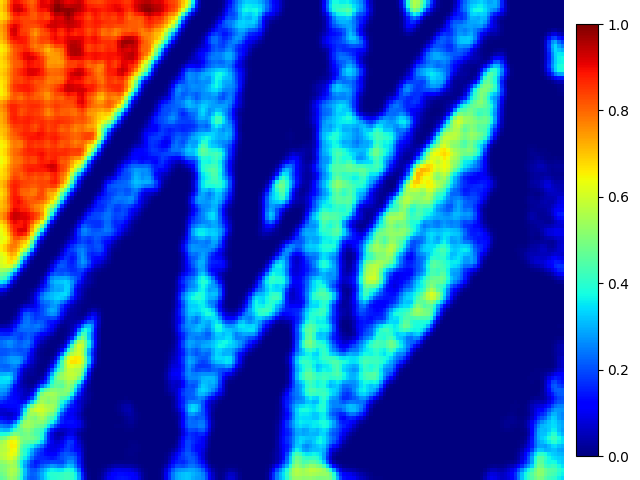
adjacency matrix

Graph connection samples

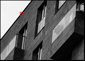
Query patch in high-quality label

Similarity matrix

adjacency matrix

Graph connection samples

Figure 3: Visualization of construction of graph connections. The regions of query patches are labeled with red boxes. The similarity matrixes and adjacency matrixes are presented in the form of heat maps. The lighter color indicates higher similarity/importance. For illustration purpose, we present some highly correlated neighbors (labeled with green boxes). One can see that our method can capture satisfied long-range correlations in highly degraded images, and the adjacency matrix accurately filters out low-important correlations.

Figure 4: Visualization of the number of neighbors in different locations. The results are normalized and presented in the form of heat maps. The lighter color indicates a larger number of neighbors. One can see that the number of neighbors changes with the frequency of image content, demonstrating that our dynamic graph method can assign neighboring nodes according to demand.

Feature aggregation. Guided by the adjacency matrix $\mathbf{A}$, the feature aggregation process is a weighted sum of all connected neighbors, which is represented as:

$$\hat{\mathbf{p}}_{i}=\sum_{j\in\mathcal{N}_{i}}\alpha_{ij}\cdot\mathbf{p}_{j}^{\prime\prime}=\sum_{j\in\mathcal{N}_{i}}\alpha_{ij}\cdot f_{node}(\mathbf{p}_{j}).$$ (10)

Then we extract all feature patches from the graph and utilize the fold operation to combine this array of updated local patches into a feature map, which can be viewed as the inverse of the unfold operation. Since there exist overlaps between feature patches, we use the average operation to deal with the overlapped areas. This strategy can also suppress the blocking effect in the final output. A global residual connection is employed in GFAM to further enhance the output. Thus, the output of GFAM is expressed as:

$$\mathbf{F}_{out}=\mathbf{F}_{in}+Fold(\{\hat{\mathbf{p}}_{i}\}_{i=1}^{N}).$$ (11)

To stabilize the training process of graph convolution, we extend our method to employ a multi-head graph to be beneficial, represented as M-GFAM in Fig. 1. The multi-heads design allows our method to jointly aggregate information from different representation subspaces at different positions. Specifically, $K$ independent heads execute the graph-based feature aggregation. Their results are concatenated together and once again projected by a $1\times 1$ convolutional layer ($f_{merge}$). Let us denote $\mathbf{F}_{out}^{k}$ as the output of the $k$-th head. The final output of M-GFAM can be calculated as $\mathbf{F}_{out}^{MH}=f_{merge}(\mathop{||}\limits_{k=1}^{K}\mathbf{F}_{out}^{k})$.

3.3 Analyze and Discussion

As mentioned previously, our improved graph model can construct robust long-range correlations based on feature patches, and the number of neighbors dynamically changes with different nodes. In this subsection, we use the visualization results in Fig. 3, 4 to demonstrate these merits.

Robust long-range correlations. In Fig. 3, we show the construction of graph connections of some query patches. The location of each query patch is labeled with a red box. For illustration purpose, we only present a limited number of neighbors (labeled with green boxes) with the highest attention weights. One can see that even the images are highly corrupted, our patch-wise graph method can still capture satisfied long-range correlations, and the adjacency matrix accurately filters out correlations with low importance.

Dynamic graph connections. Fig. 4 presents the normalized number of neighbors of each query patch at different locations. One can see that the number of neighbors follows distinct distributions over the frequency of image content, demonstrating that our dynamic graph method can adaptively select informative regions to aggregate the most useful information for each query patch.

Table 1: Quantitative results (PSNR and SSIM) of gray-scale image denoising. Best and second-best results are highlighted and underlined.

Dataset	$\bm{\sigma}$	BM3D [7]	DnCNN [49]	FFDNet [51]	N3Net [29]	NLRN [20]	GCDN [36]	DAGL (Ours)
Set12	15	32.37/0.8952	32.86/0.9031	32.75/0.9027	33.03/0.9056	33.16/0.9070	33.14/0.9072	33.28/0.9100
	25	29.96/0.8504	30.44/0.8622	30.43/0.8634	30.55/0.8648	30.80/0.8689	30.78/0.8687	30.93/0.8720
	50	26.70/0.7676	27.19/0.7829	27.31/0.7903	27.43/0.7948	27.64/0.7980	27.60/0.7957	27.81/0.8042
BSD68	15	31.07/0.8717	31.73/0.8907	31.63/0.8902	31.78/0.8927	31.88/0.8932	31.83/0.8933	31.93/0.8953
	25	28.57/0.8013	29.23/0.8278	29.19/0.8289	29.30/0.8321	29.41/0.8331	29.35/0.8332	29.46/0.8366
	50	25.62/0.6864	26.23/0.7189	26.29/0.7345	26.39/0.7293	26.47/0.7298	26.38/0.7389	26.51/0.7334
Urban100	15	32.35/0.9220	32.68/0.9255	32.43/0.9273	33.08/0.9333	33.45/0.9354	33.47/0.9358	33.79/0.9393
	25	29.71/0.8777	29.97/0.8797	29.92/0.8887	30.19/0.8925	30.94/0.9018	30.95/0.9020	31.39/0.9093
	50	25.95/0.7791	26.28/0.7874	26.52/0.8057	26.82/0.8184	27.49/0.8279	27.41/0.8160	27.97/0.8423
Parameters$\downarrow$		-	0.56M	0.49M	0.72M	0.35M	5.99M	5.62M

Urban100: img006

HQ (PSNR/SSIM)

N3Net (27.40/0.8457)

Noisy (20.60/0.5748)

NLRN (28.46/0.8688)

DnCNN (26.38/0.8052)

GCDN (28.70/0.8742)

FFDNet (27.05/0.8359)

DAGL (29.29/0.8960)

Figure 5: Visual comparison of gray-scale image denoising of various methods on one sample from Urban100 with noise level $\sigma=25$.

4 Experiments

To demonstrate the superiority of our proposed model, we apply our method to four typical image restoration tasks: synthetic image denoising, real image denoising, image demosaicing, and image compression artifacts reduction. For synthetic image denoising, image demosaicing, and image compression artifacts reduction tasks, we train our DAGL on DIV2K [34] dataset, which contains 800 high-quality images. For real image denoising, we apply the commonly used SIDD [1] dataset as the training data, which contains 160 images corrupted by realistic noise and corresponding high-quality labels. In each task, we utilize commonly used test sets for evaluation and report PSNR and SSIM [41] to evaluate the performance of each method. Our model is trained on an Nvidia Tesla V100 GPU with the initial learning rate $lr=1\times 10^{-4}$ and performs halving per 200 epochs. During training, we employ Adam optimizer, and each mini-batch contains 32 images with the size of $64\times 64$ randomly cropped from training data. The training process can be completed within two days.

4.1 Synthetic Image Denoising

We compare our proposed model with some state-of-the-art denoising methods, including some well-known denoisers, e.g., BM3D [7], DnCNN [49], and FFDNet [51], and recent competitive non-local denoisers such as N3Net [29] and NLRN [20]. Furthermore, we also compare our method with the graph-based denoiser: GCDN [36]. The standard test sets: Urban100 [15], BSD68 [22], and Set12 are applied to evaluate each method. Additive white Gaussian noise (AWGN) with different noise levels (15, 25, 50) are added to the clean images. The quantitative results (PSNR and SSIM) and the number of parameters of different methods are shown in Table 1. The visual comparison is shown in Fig. 5. One can see that our method has the best performance in all noise levels and produces higher visual quality while maintaining a moderate number of parameters.

4.2 Real Image Denoising

To further demonstrate the merits of our proposed method, we apply it to the more challenging task of real image denoising. Unlike synthetic image denoising, in this case, images are corrupted by realistic noise with unknown distribution and noise levels. We compare our method with some competitive denoisers [7, 49, 51, 42, 14] and some very recent methods [2, 43, 45, 44, 17, 30]. The commonly used DND [28] dataset is utilized for evaluation. Note that the high-quality labels of DND are not available. We get the evaluation results from the official website. The quantitative results are shown in Table 2, and we further provide a visual comparison of different methods in Fig. 6. In comparison, our algorithm recovers the actual texture and structures without compromising on the removal of noise, and our method has good robustness to both high-intensity and low-intensity noise. Even compared with top-performing methods [45, 44, 17, 30], our proposed DAGL can achieve better performance with attractive model parameters.

Table 2: The quantitative results of real image denoising on DND dataset [28].

Algorithm	Params$\downarrow$	Mode	sRGB
			PSNR$\uparrow$	SSIM$\uparrow$
BM3D [7]	-	Non-blind	34.51	0.851
CDnCNN [49]	0.67M	Blind	32.43	0.790
CFFDNet [51]	0.85M	Non-blind	37.61	0.914
TWSC [42]	-	Blind	37.94	0.940
CBDNet [14]	4.36M	Blind	38.06	0.942
RIDNet [2]	1.50M	Blind	39.23	0.952
VDNet [43]	7.82M	Blind	39.38	0.952
CycleISP [45]	2.60M	Blind	39.56	0.956
GDANet [44]	9.15M	Blind	39.58	0.954
AINDNet [17]	13.76M	Blind	39.37	0.951
DeamNet [30]	2.25M	Blind	39.70	0.953
DAGL (Ours)	5.62M	Blind	39.83	0.957

Noisy

Noisy

CBDNet [14]

CBDNet [14]

VDNet [43]

VDNet [43]

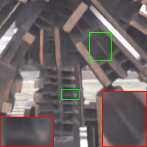
CycleISP [45]

CycleISP [45]

GDANet [44]

GDANet [44]

AINDNet [17]

AINDNet [17]

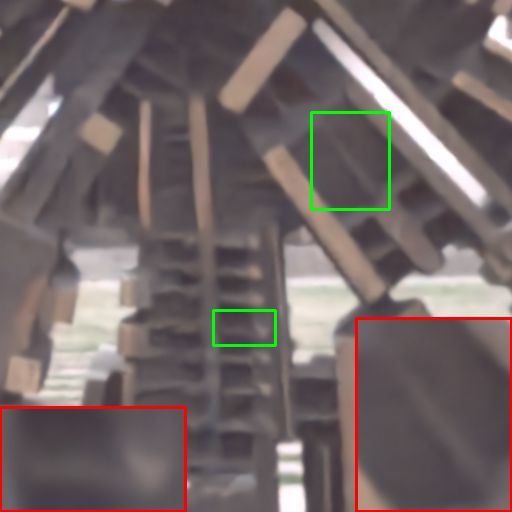
DeamNet [30]

DeamNet [30]

DAGL (Ours)

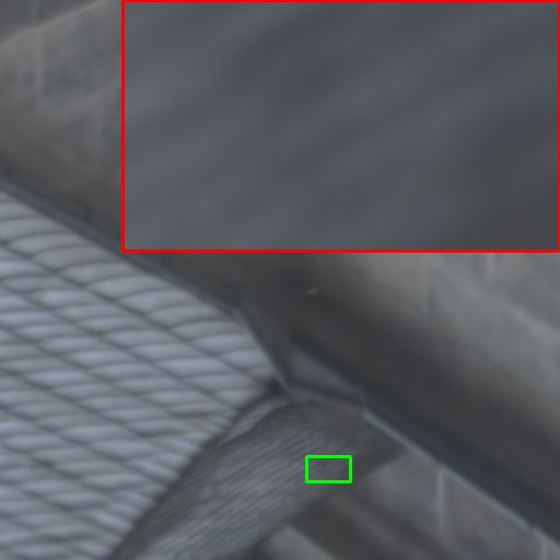
DAGL (Ours)

Figure 6: Visual comparison of real image denoising application of various methods. These noisy images come from DND [28] dataset.

Table 3: Quantitative results of image compression artifact reduction. Best and second-best results are highlighted and underlined.

Dataset	$q$	JPEG	SA-DCT [11]	ARCNN [8]	TNRD [6]	DnCNN [49]	RNAN [52]	DUN [13]	DAGL (ours)
LIVE1	10	27.77/0.7905	28.86/0.8093	28.98/0.8076	29.15/0.8111	29.19 /0.8123	29.63/0.8239	29.61/0.8232	29.70/0.8245
	20	30.07/0.8683	30.81/0.8781	31.29/0.8733	31.46/0.8769	31.59/0.8802	32.03/0.8877	31.98/0.8869	32.12/0.8887
	30	31.41/0.9000	32.08/0.9078	32.69/0.9043	32.84/0.9059	32.98/0.9090	33.45/0.9149	33.38/0.9142	33.54/0.9156
	40	32.35/0.9173	32.99/0.9240	33.63/0.9198	-/-	33.96/0.9247	34.47/0.9299	34.32/0.9289	34.53/0.9305
Classic5	10	27.82/0.7800	28.88/0.8071	29.04/0.7929	29.28/0.7992	29.40/0.8026	29.96/0.8178	29.95/0.8171	30.08/0.8196
	20	30.12/0.8541	30.92/0.8663	31.16/0.8517	31.47/0.8576	31.63/0.8610	32.11/0.8693	32.11/0.8689	32.35/0.8719
	30	31.48/0.8844	32.14/0.8914	32.52/0.8806	32.74/0.8837	32.91/0.8861	33.38/0.8924	33.33/0.8916	33.59/0.8942
	40	32.43/0.9011	33.00/0.9055	33.34/0.8953	-/-	33.77/0.9003	34.27/0.9061	34.10/0.9045	34.41/0.9069
Parameters		-	-	0.12M	-	0.56M	8.96M	10.5M	5.62M

HQ

PSNR/SSIM

HQ

PSNR/SSIM

JPEG (q=10)

25.07/0.7632

JPEG (q=10)

27.59/0.7747

TNRD [6]

26.64/0.8055

TNRD [6]

28.94/0.8111

DnCNN [49]

26.75/0.8066

DnCNN [49]

28.96/0.8122

RNAN [52]

27.58/0.8314

RNAN [52]

29.49/0.8305

DUN [13]

27.67/0.8320

DUN [13]

29.50/0.8301

DAGL (Ours)

27.82/0.8379

DAGL (Ours)

29.53/0.8316

Figure 7: Visual comparison of image compression artifact reduction application of various methods with JPEG quality q = 10.

4.3 Image Compression Artifact Reduction

For this application, we compare our DAGL with some classic methods (e.g., SA-DCT [11], ARCNN [8], TNRD [6]) and recent competitive deep-learning methods (e.g., DnCNN [49], RNAN [52], DUN [13]). To demonstrate the superiority of our DAGL, we apply the same setting as DnCNN and DUN, i.e., using a single model to handle all degradation levels. The compressed images are generated by Matlab standard JPEG encoder with quality factors $q\in\{10,20,30,40\}$. We evaluate the performance of each method on the commonly used Classic5 [11] and LIVE1 [31] test sets. The quantitative results are presented in Table 3. One can see that under the evaluation of both PSNR and SSIM, our proposed method achieves the best performance on all test sets and quality factors with a single model. In addition, the number of parameters of our DAGL is much fewer than the top-performing methods [52, 13]. The visual comparison is shown in Fig. 7, presenting the better restoration quality of our proposed DAGL.

Table 4: Quantitative comparison of image demosaicing.

Method	Params	PSNR/SSIM
		McMaster18	Kodak24	Urban100
Mosaic	-	9.17/0.1674	8.56/0.0682	7.48/0.1195
IRCNN	0.19M	37.47/0.9615	40.41/0.9807	36.64/0.9743
RNAN	8.96M	39.71/0.9725	43.09/0.9902	39.75/0.9848
DAGL	5.62M	39.84/0.9735	43.21/0.9910	40.20/0.9854

Original image

Urban100: img026

HQ

PSNR/SSIM

Mosaiced

5.98/0.0395

IRCNN [50]

33.53/0.9235

RNAN [52]

35.79/0.9519

DAGL

36.35/0.9536

Figure 8: Visual comparison of image demosaicing. Following [50], the corrupted images are generated via Matlab with Bayer mosaic.

4.4 Image Demosaicing

In this task, we compare our method with RNAN [52] and IRCNN [50] on McMaster18 [50], Kodak24, and Urban100 test sets. The quantitative result is shown in Table 4, and the visual comparison is shown in Fig. 8. One can see that the degraded images have very low quality on both subjective and objective evaluations. IRCNN and RNAN can restore the low-quality images with a good result, but our method can still make an improvement.

4.5 Ablation Study

In this subsection, we show the ablation study in Table 5 and Table 6 to investigate the effect of different components in our proposed DAGL. The experiment of ablation study is conducted on denoising task and evaluated on Urban100 test set. The noise level is set as $25$. In Table 5, we compare the performance of the variants of our proposed DAGL. In Table 6, we explore the gains brought by the number of graph-based feature aggregation modules (GFAMs) in depth (number of stages) and width (number of heads).

Patch-wise non-local correlation. The non-local correlations in our DAGL are constructed based on feature patches instead of pixels. To study the effectiveness of this design, we compare our method with the commonly used non-local neural networks [40]. Correctly, we replace the graph modules in our DAGL with non-local neural networks with one head (NL) and multiple heads (MHNL). The results are presented in Table 5. One can see that our patch-wise non-local method obviously outperforms the commonly used pixel-wise non-local method [40].

Graph attention mechanism. In this paper, we extend the graph attention mechanism to image restoration tasks. To demonstrate the effectiveness of this strategy, we replace the attention-weighted aggregation process with directly averaging, denoted as (w/o GAT) in Table 5. The performance reduction demonstrates the positive effect of the graph attention mechanism used in our DAGL.

Dynamic graph connections. Different from existing non-local image restoration methods, in our DAGL, the number of neighbors of each query patch is dynamic and adaptive. To demonstrate the effectiveness of this design, we remove the dynamic KNN module from our GFAM, leading to a fully connected non-local attention operation with a fixed number of neighbors for each query patch. This variant is denoted as (w/o THD) in Table 5. There are 0.11dB gains by using the dynamic KNN module, demonstrating the necessity of the dynamics in our graph model.

Table 5: Evaluation results about variants of DAGL on Urban100 test set ($\sigma=25$). NL and MHNL represent replacing our M-GFAM with non-local neural networks and multi-heads non-local neural networks, respectively. (w/o THD) and (w/o GAT) refer to removing dynamic KNN module and removing graph attention mechanism, respectively.

Mode	NL	MHNL	w/o THD	w/o GAT	DAGL
PSNR	30.73	30.92	31.28	30.77	31.39

Block number. In this part, we explore the gains brought by the number of graph-based feature aggregation modules (GFAM) in depth (number of stages) and width (number of heads). The results are shown in Table 6. Note that case 1 is constructed by removing all GFAM from our DAGL, resulting in a simple ResNet. From the results, we can find that our proposed GFAM can significantly boost the image restoration performance, and the performance increases with the number of heads and stages. By making a trade-off between performance and computational complexity, we employ four heads and three stages in our proposed DAGL.

Table 6: Evaluation results on Urban100 ($\sigma=25$) test set of our proposed model with different numbers of graph-based feature aggregation modules (GFAMs).

Case Index	Number of heads-stages	Params	PSNR
1	0-0	1.23M	30.43
2	1-3	2.79M	31.21
3	2-3	3.77M	31.29
4	3-3	4.74M	31.33
5 (DAGL)	4-3	5.62M	31.39
6	5-3	6.71M	31.41
7	4-4	7.22M	31.42
8	4-2	4.12M	31.28
9	4-1	2.51M	31.05

5 Conclusion

In this paper, we propose an improved graph attention model for image restoration. Unlike previous non-local image restoration methods, our model can assign an adaptive number of neighbors for each query item and construct long-range correlations based on feature patches. Furthermore, our proposed dynamic attentive graph learning can be easily extended to other computer vision tasks. Extensive experiments demonstrate that our proposed model achieves state-of-the-art performance on wide image restoration tasks: synthetic image denoising, real image denoising, image demosaicing, and compression artifact reduction.

References

- [1] Abdelrahman Abdelhamed, Stephen Lin, and Michael S Brown. A high-quality denoising dataset for smartphone cameras. In Proceedings of the IEEE Conference on Computer Vision and Pattern Recognition (CVPR), 2018.
- [2] Saeed Anwar and Nick Barnes. Real image denoising with feature attention. In Proceedings of the IEEE International Conference on Computer Vision (ICCV), 2019.
- [3] Tim Brooks, Ben Mildenhall, Tianfan Xue, Jiawen Chen, Dillon Sharlet, and Jonathan T Barron. Unprocessing images for learned raw denoising. In Proceedings of the IEEE Conference on Computer Vision and Pattern Recognition (CVPR), 2019.
- [4] Antoni Buades, Bartomeu Coll, and J-M Morel. A non-local algorithm for image denoising. In Proceedings of the IEEE Conference on Computer Vision and Pattern Recognition (CVPR), 2005.
- [5] Hanting Chen, Yunhe Wang, Tianyu Guo, Chang Xu, Yiping Deng, Zhenhua Liu, Siwei Ma, Chunjing Xu, Chao Xu, and Wen Gao. Pre-trained image processing transformer. In Proceedings of the IEEE Conference on Computer Vision and Pattern Recognition (CVPR), 2021.
- [6] Yunjin Chen and Thomas Pock. Trainable nonlinear reaction diffusion: A flexible framework for fast and effective image restoration. IEEE Transactions on Pattern Analysis and Machine Intelligence (TPAMI), 39(6):1256–1272, 2016.
- [7] Kostadin Dabov, Alessandro Foi, Vladimir Katkovnik, and Karen Egiazarian. Image denoising by sparse 3-D transform-domain collaborative filtering. IEEE Transactions on Image Processing (TIP), 16(8):2080–2095, 2007.
- [8] Chao Dong, Yubin Deng, Chen Change Loy, and Xiaoou Tang. Compression artifacts reduction by a deep convolutional network. In Proceedings of the IEEE International Conference on Computer Vision (ICCV), 2015.
- [9] Weisheng Dong, Xin Li, Lei Zhang, and Guangming Shi. Sparsity-based image denoising via dictionary learning and structural clustering. In Proceedings of the IEEE Conference on Computer Vision and Pattern Recognition (CVPR), 2011.
- [10] Michael Elad and Michal Aharon. Image denoising via sparse and redundant representations over learned dictionaries. IEEE Transactions on Image Processing (TIP), 15(12):3736–3745, 2006.
- [11] Alessandro Foi, Vladimir Katkovnik, and Karen Egiazarian. Pointwise shape-adaptive DCT for high-quality denoising and deblocking of grayscale and color images. IEEE Transactions on Image Processing (TIP), 16(5):1395–1411, 2007.
- [12] Xueyang Fu, Qi Qi, Zheng-Jun Zha, Xinghao Ding, Feng Wu, and John Paisley. Successive graph convolutional network for image de-raining. International Journal of Computer Vision (IJCV), 129(5):1691–1711, 2021.
- [13] Xueyang Fu, Menglu Wang, Xiangyong Cao, Xinghao Ding, and Zheng-Jun Zha. A model-driven deep unfolding method for jpeg artifacts removal. IEEE Transactions on Neural Networks and Learning Systems (TNNLS), 2021.
- [14] Shi Guo, Zifei Yan, Kai Zhang, Wangmeng Zuo, and Lei Zhang. Toward convolutional blind denoising of real photographs. In Proceedings of the IEEE Conference on Computer Vision and Pattern Recognition (CVPR), 2019.
- [15] Jia-Bin Huang, Abhishek Singh, and Narendra Ahuja. Single image super-resolution from transformed self-exemplars. In Proceedings of the IEEE Conference on Computer Vision and Pattern Recognition (CVPR), 2015.
- [16] Sergey Ioffe and Christian Szegedy. Batch normalization: Accelerating deep network training by reducing internal covariate shift. In Proceedings of the International Conference on Machine Learning (ICML), 2015.
- [17] Yoonsik Kim, Jae Woong Soh, Gu Yong Park, and Nam Ik Cho. Transfer learning from synthetic to real-noise denoising with adaptive instance normalization. In Proceedings of the IEEE Conference on Computer Vision and Pattern Recognition (CVPR), 2020.
- [18] Stamatios Lefkimmiatis. Non-local color image denoising with convolutional neural networks. In Proceedings of the IEEE Conference on Computer Vision and Pattern Recognition (CVPR), 2017.
- [19] Stamatios Lefkimmiatis. Universal denoising networks: a novel CNN architecture for image denoising. In Proceedings of the IEEE Conference on Computer Vision and Pattern Recognition (CVPR), 2018.
- [20] Ding Liu, Bihan Wen, Yuchen Fan, Chen Change Loy, and Thomas S Huang. Non-local recurrent network for image restoration. In Proceedings of the Advances in Neural Information Processing Systems (NeurIPS), 2018.
- [21] Zhilei Liu, Le Li, Yunpeng Wu, and Cuicui Zhang. Facial expression restoration based on improved graph convolutional networks. In International Conference on Multimedia Modeling, 2020.
- [22] David Martin, Charless Fowlkes, Doron Tal, and Jitendra Malik. A database of human segmented natural images and its application to evaluating segmentation algorithms and measuring ecological statistics. In Proceedings of IEEE International Conference on Computer Vision (ICCV), 2001.
- [23] Yiqun Mei, Yuchen Fan, Yuqian Zhou, Lichao Huang, Thomas S Huang, and Honghui Shi. Image super-resolution with cross-scale non-local attention and exhaustive self-exemplars mining. In Proceedings of the IEEE Conference on Computer Vision and Pattern Recognition (CVPR), 2020.
- [24] Chong Mou, Jian Zhang, Xiaopeng Fan, Hangfan Liu, and Ronggang Wang. COLA-Net: Collaborative attention network for image restoration. IEEE Transactions on Multimedia (TMM), 2021.
- [25] Vinod Nair and Geoffrey E Hinton. Rectified linear units improve restricted boltzmann machines. In Proceedings of the International Conference on Machine Learning (ICML), 2010.
- [26] Stanley Osher, Martin Burger, Donald Goldfarb, Jinjun Xu, and Wotao Yin. An iterative regularization method for total variation-based image restoration. Multiscale Modeling & Simulation, 4(2):460–489, 2005.
- [27] Francesca Pistilli, Giulia Fracastoro, Diego Valsesia, and Enrico Magli. Learning graph-convolutional representations for point cloud denoising. In Proceedings of the European Conference on Computer Vision (ECCV), 2020.
- [28] Tobias Plotz and Stefan Roth. Benchmarking denoising algorithms with real photographs. In Proceedings of the IEEE Conference on Computer Vision and Pattern Recognition (CVPR), 2017.
- [29] Tobias Plötz and Stefan Roth. Neural nearest neighbors networks. In Proceedings of the Advances in Neural Information Processing Systems (NeurIPS), 2018.
- [30] Chao Ren, Xiaohai He, Chuncheng Wang, and Zhibo Zhao. Adaptive consistency prior based deep network for image denoising. In Proceedings of the IEEE Conference on Computer Vision and Pattern Recognition (CVPR), 2021.
- [31] HR Sheikh. Live image quality assessment database release 2. http://live. ece. utexas. edu/research/quality, 2005.
- [32] Martin Simonovsky and Nikos Komodakis. Dynamic edge-conditioned filters in convolutional neural networks on graphs. In Proceedings of the IEEE Conference on Computer Vision and Pattern Recognition (CVPR), 2017.
- [33] Ying Tai, Jian Yang, Xiaoming Liu, and Chunyan Xu. MemNet: A persistent memory network for image restoration. In Proceedings of the IEEE International Conference on Computer Vision (ICCV), 2017.
- [34] Radu Timofte, Eirikur Agustsson, Luc Van Gool, Ming-Hsuan Yang, and Lei Zhang. Ntire 2017 challenge on single image super-resolution: Methods and results. In Proceedings of the IEEE Conference on Computer Vision and Pattern Recognition Workshops (CVPRW), 2017.
- [35] Diego Valsesia, Giulia Fracastoro, and Enrico Magli. Image denoising with graph-convolutional neural networks. In Proceedings of the IEEE International Conference on Image Processing, 2019.
- [36] Diego Valsesia, Giulia Fracastoro, and Enrico Magli. Deep graph-convolutional image denoising. IEEE Transactions on Image Processing (TIP), 29:8226–8237, 2020.
- [37] Ashish Vaswani, Noam Shazeer, Niki Parmar, Jakob Uszkoreit, Llion Jones, Aidan N Gomez, Lukasz Kaiser, and Illia Polosukhin. Attention is all you need. In Proceedings of the Advances in Neural Information Processing Systems (NeurIPS), 2017.
- [38] Petar Veličković, Guillem Cucurull, Arantxa Casanova, Adriana Romero, Pietro Liò, and Yoshua Bengio. Graph attention networks. In Proceedings of the International Conference on Learning Representations (ICLR), 2018.
- [39] Tianyang Wang, Mingxuan Sun, and Kaoning Hu. Dilated deep residual network for image denoising. In Proceedings of the 2017 IEEE 29th International Conference on Tools with Artificial Intelligence, 2017.
- [40] Xiaolong Wang, Ross Girshick, Abhinav Gupta, and Kaiming He. Non-local neural networks. In Proceedings of the IEEE Conference on Computer Vision and Pattern Recognition (CVPR), 2018.
- [41] Zhou Wang, Alan C Bovik, Hamid R Sheikh, and Eero P Simoncelli. Image quality assessment: From error visibility to structural similarity. IEEE Transactions on Image Processing (TIP), 13(4):600–612, 2004.
- [42] Jun Xu, Lei Zhang, and David Zhang. A trilateral weighted sparse coding scheme for real-world image denoising. In Proceedings of the European Conference on Computer Vision (ECCV), 2018.
- [43] Zongsheng Yue, Hongwei Yong, Qian Zhao, Deyu Meng, and Lei Zhang. Variational denoising network: Toward blind noise modeling and removal. In Proceedings of the Advances in Neural Information Processing Systems (NeurIPS), 2019.
- [44] Zongsheng Yue, Qian Zhao, Lei Zhang, and Deyu Meng. Dual adversarial network: Toward real-world noise removal and noise generation. In Proceedings of the European Conference on Computer Vision (ECCV), 2020.
- [45] Syed Waqas Zamir, Aditya Arora, Salman Khan, Munawar Hayat, Fahad Shahbaz Khan, Ming-Hsuan Yang, and Ling Shao. Cycleisp: Real image restoration via improved data synthesis. In Proceedings of the IEEE Conference on Computer Vision and Pattern Recognition (CVPR), 2020.
- [46] Jian Zhang, Chen Zhao, and Wen Gao. Optimization-inspired compact deep compressive sensing. IEEE Journal of Selected Topics in Signal Processing, 14(4):765–774, 2020.
- [47] Jian Zhang, Debin Zhao, and Wen Gao. Group-based sparse representation for image restoration. IEEE Transactions on Image Processing (TIP), 23(8):3336–3351, 2014.
- [48] Jian Zhang, Debin Zhao, Ruiqin Xiong, Siwei Ma, and Wen Gao. Image restoration using joint statistical modeling in a space-transform domain. IEEE Transactions on Circuits and Systems for Video Technology, 24(6):915–928, 2014.
- [49] Kai Zhang, Wangmeng Zuo, Yunjin Chen, Deyu Meng, and Lei Zhang. Beyond a Gaussian denoiser: Residual learning of deep CNN for image denoising. IEEE Transactions on Image Processing (TIP), 26(7):3142–3155, 2017.
- [50] Kai Zhang, Wangmeng Zuo, Shuhang Gu, and Lei Zhang. Learning deep CNN denoiser prior for image restoration. In Proceedings of the IEEE Conference on Computer Vision and Pattern Recognition (CVPR), 2017.
- [51] Kai Zhang, Wangmeng Zuo, and Lei Zhang. FFDNet: toward a fast and flexible solution for CNN-based image denoising. IEEE Transactions on Image Processing (TIP), 27(9):4608–4622, 2018.
- [52] Yulun Zhang, , Kunpeng Li, Bineng Zhong, and Yun Fu. Residual non-local attention networks for image restoration. In Proceedings of the International Conference on Learning Representations (ICLR), 2019.
- [53] Yulun Zhang, Kunpeng Li, Kai Li, Lichen Wang, Bineng Zhong, and Yun Fu. Image super-resolution using very deep residual channel attention networks. In Proceedings of the European Conference on Computer Vision (ECCV), 2018.
- [54] Chen Zhao, Siwei Ma, Jian Zhang, Ruiqin Xiong, and Wen Gao. Video compressive sensing reconstruction via reweighted residual sparsity. IEEE Transactions on Circuits and Systems for Video Technology, 27(6):1182–1195, 2016.
- [55] Chen Zhao, Jian Zhang, Siwei Ma, Xiaopeng Fan, Yongbing Zhang, and Wen Gao. Reducing image compression artifacts by structural sparse representation and quantization constraint prior. IEEE Transactions on Circuits and Systems for Video Technology, 27(10):2057–2071, 2016.
- [56] Maria Zontak and Michal Irani. Internal statistics of a single natural image. In Proceedings of the IEEE Conference on Computer Vision and Pattern Recognition (CVPR), 2011.