$SU(2,1)/(SU(2)\times U(1))~{}B-L$ Higgs Inflation

Abstract

We present a realization of Higgs inflation within Supergravity which is largely tied to the existence of a pole of order two in the kinetic term of the inflaton field. This pole arises due to the selected Kaehler potential which parameterizes the $SU(2,1)/(SU(2)\times U(1))$ manifold with scalar curvature ${\cal R}_{21}=-6/N$. The associated superpotential includes, in addition to the Higgs superfields, a stabilizer superfield, respects a $B-L$ gauge and an $R$ symmetries and contains the first allowed nonrenormalizable term. If the coefficient of this term is almost equal to that of the others within about $10^{-5}$ and $N=2$, the inflationary observables can be done compatible with the present data. The tuning can be eluded if we modify the Kaehler potential associated with the manifold above. In this case, inflation can be realized with just renormalizable superpotential terms and results to higher tensor-to-scalar ratios as $N$ approaches its maximum at $N\simeq 80$.

1 Introduction

One of the major challenges in the are(n)a of inflationary model building [1] is the identification of the inflaton – i.e., the scalar field causing inflation – with one of the fields already present in the fundamental theory. According to an economical, predictive and highly attractive set-up, the inflaton could play, at the end of its inflationary evolution, the role of a Higgs field [2, 3, 4, 8, 9, 7, 5, 6] – obviously we do not restrict our attention only to the electroweak Higgs [3]. The relevant models (for a more complete list see Ref. [10] and references therein) may be called Higgs inflation (HI) for short. We find it technically convenient to exemplify HI in our talk taking as reference theory an “elementary” Grand Unified Theory (GUT) based on the gauge group $G_{B-L}=G_{\rm SM}\times U(1)_{B-L}$ – where ${G_{\rm SM}}$ is the gauge group of the Standard Model (SM), $B$ and $L$ denote baryon and lepton number respectively. Despite its simplicity, $G_{B-L}$ is strongly motivated by neutrino physics and leptogenesis mechanisms – see e.g. Ref. [11, 7].

The spontaneous breaking of $U(1)_{B-L}$ requires the introduction of a Higgs fields $\Phi$ in a non-Supersymmetric (SUSY) framework or a conjugate pair of Higgs fields $\Phi$ and $\bar{\Phi}$ in a SUSY context. The Higgsflaton [12] may be identified with the radial part of these fields and is expected to obey a $\phi^{4}$ potential. Due to inconsistency of that model with a number of observational and theoretical requirements described in Sec. 1.2, we are obliged to invoke some non-minimality. We below review – in Sec. 1.1 – the formulation of generalized non-minimal HI in a non-SUSY framework. Then – in Sec. 1.3 – we constrain the parameters of two possible models, called E and T model in Ref. [13]. In the next sections we investigate the supersymmetrization of T model [14, 15] HI, following the approach of Ref. [10].

Throughout the text, the subscript $,\chi$ denotes derivation with respect to (w.r.t) the field $\chi$, charge conjugation is denoted by a star (^∗) and we use units where the reduced Planck scale $m_{\rm P}=2.43\cdot 10^{18}~{}{\mbox{\rm GeV}}$ is set equal to unity.

1.1 Formulating Non-SUSY Higgs Inflation

The potential of the inflaton $\phi$ (i.e., the radial component of $\Phi$ assuming that the angular direction is somehow stabilized) has to be of the well-known form

$$V_{\rm HI}=\lambda^{2}(\phi^{2}-M^{2})^{2}/16\simeq\lambda^{2}\phi^{4}/16\>\>\>\mbox{for}\>\>\>M\ll m_{\rm P}=1.$$ (1)

The corresponding action in the Jordan frame (JF), takes the form:

$${\sf S}=\int d^{4}x\sqrt{-\mathfrak{g}}\left(-\frac{f_{\mathcal{R}}}{2}\mathcal{R}+\frac{f_{\rm K}}{2}g^{\mu\nu}\partial_{\mu}\phi\partial_{\nu}\phi-V_{\rm HI}(\phi)+\cdots\right),$$ (2a)

where $$\mathfrak{g} g^{\mu\nu} (+,-,-,-) \widehat{\mathcal{R}} \langle{f_{\mathcal{R}}}\rangle\simeq 1 f_{\rm K}(\phi) \phi \widehat{g}_{\mu\nu}=f_{\mathcal{R}}\,g_{\mu\nu} {\sf S}$$ is the determinant of the background Friedmann-Robertson-Walker metric with signature , is the space-time Ricci scalar, to guarantee the ordinary Einstein gravity at low energy and we allow for a kinetic mixing through the function . The ellipsis includes the gauge interactions of which may be neglected at a tree level treatment. By performing a conformal transformation [2] according to which we define the Einstein frame (EF) metric we can write in the EF as follows

$${\sf S}=\int d^{4}x\sqrt{-\widehat{\mathfrak{g}}}\left(-\frac{1}{2}\widehat{\mathcal{R}}+\frac{1}{2}\widehat{g}^{\mu\nu}\partial_{\mu}\widehat{\phi}\partial_{\nu}\widehat{\phi}-\widehat{V}_{\rm HI}(\widehat{\phi})+\cdots\right),$$ (2b)

where hat is used to denote quantities defined in the EF. We also introduce the EF potential, $\widehat{V}_{\rm HI}$, and canonically normalized field, $\widehat{\phi}$, derived as follows

$$\mbox{\sf(a)}\>\>\widehat{V}_{\rm HI}=\frac{V_{\rm HI}}{f_{\mathcal{R}}^{2}}\>\>\>\mbox{and}\>\>\>\mbox{\sf(b)}\>\>\frac{d\widehat{\phi}}{d\phi}=J=\sqrt{\frac{f_{\rm K}}{f_{\mathcal{R}}}+{3\over 2}\left({f_{R,\phi}\over f_{\mathcal{R}}}\right)^{2}}\,.$$ (3)

Naively, we expect that $f_{\mathcal{R}}$ affects both $J$ and $\widehat{V}_{\rm HI}$ whereas $f_{\rm K}$ only $J$. Therefore, a suitable choice of $f_{\mathcal{R}}$ [2, 3, 4, 16, 13] can lead to a plateau convenient for driving HI. However, a plateau may also appear expressing $V_{\rm HI}$ in terms of $\widehat{\phi}$ [14, 15] without the aid of $f_{\mathcal{R}}$.

1.2 Inflationary Observables – Constraints

The analysis of HI can be performed exclusively in the EF using the standard slow-roll approximation as analyzed below, together with the relevant observational and theoretical requirements that should be imposed.

1.2.1

The number of e-foldings $N_{\star}$ that the scale $k_{\star}=0.05/{\rm Mpc}$ experiences during HI must be enough for the resolution of the problems of standard Big Bang, i.e., [17]

$$N_{\star}=\int_{\widehat{\phi}_{\rm f}}^{\widehat{\phi}_{\star}}d\widehat{\phi}\frac{\widehat{V}_{\rm HI}}{\widehat{V}_{\rm HI,\widehat{\phi}}}\simeq 61.5+\frac{1}{4}\ln\frac{\widehat{V}_{\rm HI}(\widehat{\phi}_{\star})^{2}}{g_{\rm rh*}^{1/3}\widehat{V}_{\rm HI}(\widehat{\phi}_{\rm f})}\simeq 55,$$ (4a)

where $$g_{\rm rh*}=228.75 \widehat{\phi}_{\star} \widehat{\phi} k_{\star} \widehat{\phi}_{\rm f} \widehat{\phi}$$ and is the value of when crosses the inflationary horizon whereas is the value of at the end of HI, which can be found, in the slow-roll approximation, from the condition

$${\sf max}\{\widehat{\epsilon}(\phi_{\rm f}),|\widehat{\eta}(\phi_{\rm f})|\}=1,\>\>\>~{}\mbox{where}\>\>\>\widehat{\epsilon}={1\over 2}\left(\frac{\widehat{V}_{\rm HI,\widehat{\phi}}}{\widehat{V}_{\rm HI}}\right)^{2}\>\>\>\mbox{and}\>\>\>\widehat{\eta}=\frac{\widehat{V}_{\rm HI,\widehat{\phi}\widehat{\phi}}}{\widehat{V}_{\rm HI}}\,.$$ (4b)

1.2.2

The amplitude $A_{\rm s}$ of the power spectrum of the curvature perturbations generated by $\phi$ at $k_{\star}$ has to be consistent with data [17], i.e.,

$$A_{\rm s}=\>\frac{1}{12\,\pi^{2}}\;\frac{\widehat{V}_{\rm HI}(\widehat{\phi}_{\star})^{3}}{\widehat{V}_{\rm HI,\widehat{\phi}}(\widehat{\phi}_{\star})^{2}}\simeq 2.105\cdot 10^{-9}\,.$$ (5)

1.2.3

The remaining inflationary observables (the spectral index $n_{\rm s}$, its running $\alpha_{\rm s}$, and the tensor-to-scalar ratio $r$) have to be consistent with the data [18, 19], i.e.,

$$\mbox{\sf(a)}\>\>n_{\rm s}=0.967\pm 0.0074\>\>\>~{}\mbox{and}\>\>\>~{}\mbox{\sf(b)}\>\>r\leq 0.07,$$ (6)

at 95$\%$ confidence level (c.l.) – pertaining to the $\Lambda$CDM$+r$ framework with $|\alpha_{\rm s}|\ll 0.01$. These observables are estimated through the relations

$$\mbox{\sf(a)}\>\>n_{\rm s}=\>1-6\widehat{\epsilon}_{\star}\ +\ 2\widehat{\eta}_{\star},\>\>\>\mbox{\sf(b)}\>\>\alpha_{\rm s}=\frac{2}{3}\left(4\widehat{\eta}^{2}-(n_{\rm s}-1)^{2}\right)-2\widehat{\xi}_{\star}\>\>\>~{}\mbox{and}\>\>\>~{}\mbox{\sf(c)}\>\>r=16\widehat{\epsilon}_{\star}\,,$$ (7)

with $\widehat{\xi}={\widehat{V}_{\rm HI,\widehat{\phi}}\widehat{V}_{\rm HI,\widehat{\phi}\widehat{\phi}\widehat{\phi}}/\widehat{V}_{\rm HI}^{2}}$ – the variables with subscript $\star$ are evaluated at $\phi=\phi_{\star}$.

1.2.4

The effective theory describing HI has to remain valid up to a UV cutoff scale $\Lambda_{\rm UV}\simeq m_{\rm P}$ to ensure the stability of our inflationary solutions [20], i.e.,

$$\mbox{\sf(a)}\>\>\widehat{V}_{\rm HI}(\phi_{\star})^{1/4}\leq\Lambda_{\rm UV}\>\>\>~{}\mbox{and}\>\>\>~{}\mbox{\sf(b)}\>\>\phi_{\star}\leq\Lambda_{\rm UV}.$$ (8)

1.3 Non-Minimal versus Pole-Induced HI

The minimal model of HI defined by $\widehat{V}_{\rm HI}$ in Eq. (1), $f_{\rm K}=1$ and $f_{\mathcal{R}}=1$ is by now observationally excluded [18] since it yields $n_{\rm s}\simeq 0.947$ and $r\simeq 0.28$ far away from the restrictions in Eq. (6). Consequently, we have to invoke some kind of non-minimality to reconcile HI based on $\widehat{V}_{\rm HI}$ in Eq. (1) with data. Actually, there are two available sources of non-minimality as shown in Eq. (2a). One due to $f_{\cal R}\neq 1$ and one due to $f_{\rm K}(\phi)\neq 1$. Below we review two observationally viable models of HI which are based on successful choices of either functions [13] – for HI implemented with a synergy between non-minimal $f_{\rm K}$ and $f_{\mathcal{R}}$ see Ref. [6, 7, 9]:

1.3.1 (Standard) Non-Minimal or E-Model HI

It can be realized [3, 2, 4], if we adopt $f_{\rm K}=1$ and $f_{\mathcal{R}}=1+c_{\mathcal{R}}\phi^{2}$. From Eq. (3) we obtain

$$V_{\rm HI}\simeq\frac{\lambda^{2}}{16c_{\mathcal{R}}^{2}}\>\>\>\mbox{and}\>\>\>J\simeq\frac{\sqrt{6}c_{\mathcal{R}}\phi}{f_{\mathcal{R}}}~{}~{}~{}\stackrel{{\scriptstyle\mbox{\footnotesize(3b)}}}{{\Rightarrow}}~{}~{}~{}\widehat{\phi}=\sqrt{\frac{3}{2}}\ln f_{\mathcal{R}}\>\>\>\mbox{or}\>\>\>\phi=\frac{1}{\sqrt{c_{\mathcal{R}}}}\left(e^{\sqrt{\frac{2}{3}}\widehat{\phi}}-1\right)^{1/2},$$ (9)

i.e., $\widehat{V}_{\rm HI}$ exhibits an almost flat plateau, whereas $\phi\sim e^{\widehat{\phi}}$ and thus, the name E-model HI. Indeed, from Eqs. (4a) and (4b) we find

$$\widehat{\epsilon}\simeq{4/3c_{\mathcal{R}}^{2}\phi^{4}},\>\>\>\widehat{\eta}\simeq-{4/3c_{\mathcal{R}}\phi^{2}}\>\>\>\mbox{and}\>\>\>N_{\star}\simeq{3c_{\mathcal{R}}\phi_{*}^{2}/4}\,.$$ (10a)

Therefore, $$\phi_{\rm f} \phi_{\star}$$ and are found from the condition of Eq. (4b) and the last equality above, as follows

$$\phi_{\rm f}=(4/3c_{\mathcal{R}}^{2})^{1/4}\>\>\>\mbox{and}\>\>\>\phi_{\star}=(4N_{\star}/3c_{\mathcal{R}})^{1/2}.$$ (10b)

Consequently, HI can be achieved even with subplanckian $\phi$ values for $c_{\mathcal{R}}\gtrsim(4\widehat{N}_{*}/3)^{1/2}$. Also the normalization of Eq. (5) implies the following relation between $c_{\mathcal{R}}$ and $\lambda$

$$\lambda\simeq{6}\sqrt{2A_{\rm s}}\pi c_{\mathcal{R}}/{N_{\star}}\>\Rightarrow\>c_{\mathcal{R}}\simeq 2.25\cdot 10^{4}\lambda\>\>\>\mbox{for}\>\>\>N_{\star}\simeq 55.$$ (11)

From Eq. (7) we compute the remaining observables

$$n_{\rm s}\simeq 1-{2/N_{\star}}\simeq 0.965,\>\>\>\alpha_{\rm s}\simeq{-2/N_{\star}^{2}}\simeq-6.4\cdot 10^{-4}\>\>\>\mbox{and}\>\>\>r\simeq{12/N_{\star}^{2}}\simeq 4\cdot 10^{-3},$$ (12)

which are $c_{\mathcal{R}}$-independent and in agreement with Eq. (6).

Although quite compelling, this model of HI is not consistent with Eq. (8) since $\widehat{V}_{\rm HI}^{1/4}\gg\Lambda_{\rm UV}=m_{\rm P}/c_{\mathcal{R}}\ll m_{\rm P}$ [20]. This fact can be easily seen if we expand the second and third term of ${\sf S}$ in the right-hand side of Eq. (2b) about $\langle{\phi}\rangle=0$ with results

$$J^{2}\dot{\phi}^{2}=\left(1-c_{\mathcal{R}}\widehat{\phi}^{2}+6c_{\mathcal{R}}^{2}\widehat{\phi}^{2}+c_{\mathcal{R}}^{2}\widehat{\phi}^{4}-\cdots\right)\dot{}\widehat{\phi}^{2}~{}~{}\mbox{and}~{}~{}\widehat{V}_{\rm HI}=\frac{\lambda^{2}\widehat{\phi}^{4}}{2}\left(1-2c_{\mathcal{R}}\widehat{\phi}^{2}+3c_{\mathcal{R}}^{2}\widehat{\phi}^{4}-\cdots\right)\cdot$$ (13)

Since the term which yields the smallest denominator for $c_{\mathcal{R}}>1$ is $6c_{\mathcal{R}}^{2}\widehat{\phi}^{2}$ we find $\Lambda_{\rm UV}=m_{\rm P}/c_{\mathcal{R}}\ll m_{\rm P}$ and so the effective theory breaks down above it. For solutions proposed to overcome this inconsistency rendering, mostly, the model less predictive see Ref. [5, 6] and references therein.

1.3.2 Pole-Induced or T-Model HI

In this case – cf. Ref. [14, 15, 10] – we introduce a pole in $f_{\rm K}$, i.e., we set $f_{\mathcal{R}}=1$ and $f_{\rm K}=2N/f_{\rm P}^{2}$ with $f_{\rm P}=1-\phi^{2}$ and $N>0$ – possible coefficient of $\phi$ in $f_{\rm P}$ can be trivially absorbed by a field redefinition. From Eq. (3) we obtain

$$V_{\rm HI}=\widehat{V}_{\rm HI}~{}~{}~{}\mbox{and}~{}~{}~{}J=\frac{\sqrt{2N}}{f_{\rm P}}\>\>\stackrel{{\scriptstyle\mbox{\footnotesize(3b)}}}{{\Rightarrow}}\>\>\widehat{\phi}=\sqrt{\frac{N}{2}}\ln\frac{(1+\phi)}{(1-\phi)}\>\>\>\mbox{or}\>\>\>\phi=\tanh\frac{\widehat{\phi}}{\sqrt{2N}},$$ (14)

i.e., we here obtain $\phi\sim\tanh\widehat{\phi}$ and hence, the name T-model (TM₄) HI. If we express $V_{\rm HI}$ in terms of $\widehat{\phi}$, we easily infer that it experiences a stretching for $\widehat{\phi}>1$ which results to a plateau [14, 10]. Applying Eqs. (4a) and (4b), the slow-roll parameters and $N_{\star}$ read

$$\widehat{\epsilon}\simeq{16f_{\rm P}^{2}/N\phi^{2}},\>\>\>\widehat{\eta}\simeq{8f_{\rm P}(3-5\phi^{2})/N\phi^{2}}\>\>\>\mbox{and}\>\>\>N_{\star}\simeq{N\phi_{\star}^{2}/4f_{\rm p\star}}.$$ (15a)

Since $$f_{\rm p\star} N_{\star} \phi_{\star} \phi_{\star}$$ appears in the denominator, increases drastically as approaches unity, assuring thereby the achievement of efficient HI. Imposing the condition of Eq. (4b) and solving then the latter equation w.r.t , we arrive at

$$\phi_{\star}=\sqrt{4N_{\star}}/\sqrt{4N_{\star}+N}\sim 1\gg\phi_{\rm f},$$ (15b)

i.e., HI is attained for $\phi<1$ thanks to the location of the pole at $\phi=1$. On the other hand, Eq. (5) implies

$$\lambda\simeq{4\sqrt{6NA_{\rm s}}\pi/N_{\star}}\>\Rightarrow\>\lambda\sim 10^{-5}\>\>\>\mbox{for}\>\>\>N_{\star}\simeq 55.$$ (16)

Applying Eq. (7) we find that the inflationary observables can be consistent with Eq. (6). Indeed,

$$n_{\rm s}\simeq 1-{2/N_{\star}}\simeq 0.965,\>\>\>\alpha_{\rm s}\simeq-{2/N_{\star}^{2}}=9.5\cdot 10^{-4}\>\>\>\mbox{and}\>\>\>r\simeq{4N/N_{\star}^{2}}\leq 0.07\>\>\>\Rightarrow\>\>\>N\leq 80,$$ (17)

where the last bound is numerically obtained [10]. Obviously, there is no problem with the effective theory here but just a tuning related to the initial conditions – see Sec. 3.3 below.

TM₄ is mostly analyzed assuming a gauge-singlet inflaton – cf. Ref. [14, 15]. We below describe its possible realization by a (gauge non-singlet) Higgsflaton in the context of Supergravity (SUGRA) – see Sec. 2 – and then, in Sec. 3, we analyze the inflationary behavior of the proposed models. We conclude summarizing our results in Sec. 4.

2 Supergravity Embeddings

TM₄ $B-L$ HI can be supersymmetrized if we employ three chiral superfields, a conjugate pair of Higgs superfields – $z^{1}=\Phi$ and $z^{2}=\bar{\Phi}$ – oppositely charged under the gauged $U(1)_{B-L}$, and a gauge singlet $z^{3}=S$ which plays the role of “stabilizer” superfield.

In Sec. 2.1 we present the basic formulation of a $B-L$ Higgs theory within SUGRA and then we motivate in Sec. 2.2 and 2.3 the necessary ingredients for realizing $B-L$ pole-induced HI and describe in Sec. 2.4 the geometry of the adopted moduli space.

2.1 General Setup

Denoting the scalar components of the various superfields by the same superfield symbol, the EF action for $z^{\alpha}$’s can be written as

$${\sf S}=\int d^{4}x\sqrt{-\widehat{\mathfrak{g}}}\left(-\frac{1}{2}\widehat{\mathcal{R}}+K_{{\alpha}{\bar{\beta}}}\widehat{g}^{\mu\nu}D_{\mu}z^{\alpha}D_{\nu}z^{*{\bar{\beta}}}-\widehat{V}\right),$$ (18a)

where the kinetic mixing is controlled by the Kähler metric and the covariant derivatives for scalar fields $$z^{\alpha}$$ defined respectively as

$$K_{{\alpha}{\bar{\beta}}}={K_{,z^{\alpha}z^{*{\bar{\beta}}}}}>0\>\>\>\mbox{and}\>\>\>D_{\mu}z^{\alpha}=\partial_{\mu}z^{\alpha}+igA_{BL\mu}(B-L)z^{\alpha},$$ (18b)

where $$g A_{BL\mu} \widehat{V} K W$$ is the unified gauge coupling constant, is the corresponding gauge field. On the other hand, the EF potential , depends on the Kähler potential and superpotential, , as shown from its explicit formula

$$\widehat{V}=\widehat{V}_{\rm F}+\widehat{V}_{\rm D}\>\>\>\mbox{with}\>\>\>\widehat{V}_{\rm F}=e^{K}\left(K^{{\alpha}{\bar{\beta}}}{\rm F}_{\alpha}{\rm F}^{*}_{\bar{\beta}}-3{|W|^{2}}\right)\>\>\>\mbox{and}\>\>\>\widehat{V}_{\rm D}={1\over 2}g^{2}{\rm D}_{(B-L)}^{2}\cdot$$ (18c)

Here, a trivial gauge kinetic function is adopted. Also we use the shorthand

$$K^{{\alpha}{\bar{\beta}}}K_{{\alpha}\bar{\gamma}}=\delta^{\bar{\beta}}_{\bar{\gamma}},\>\>{\rm F}_{\alpha}=W_{,z^{\alpha}}+K_{,z^{\alpha}}W~{}~{}\mbox{and}~{}~{}{\rm D}_{B-L}=z_{\alpha}(B-L)K^{\alpha}~{}~{}\mbox{with}~{}~{}K^{{\alpha}}={K_{,z^{\alpha}}}\cdot$$ (18d)

In this talk we concentrate on HI driven by $\widehat{V}_{\rm F}$ along a D-flat direction, and therefore we ignore any contribution from $\widehat{V}_{\rm D}$.

The interference of $K$ both in the $\bar{\Phi}-\Phi$ kinetic mixing and in $\widehat{V}_{\rm F}$ consists a complication w.r.t the non-SUSY case since the presence of the pole in the kinetic terms affects also $\widehat{V}_{\rm F}$ – cf. Ref. [21]. This is rather problematic and we show below how we arrange it in two ways.

2.2 Superpotential

Our proposal is based on the following superpotential[22]

$$W=\lambda S\left(\bar{\Phi}\Phi-M^{2}/2\right)/2-\lambda^{\prime}S(\bar{\Phi}\Phi)^{2},$$ (19)

where $\lambda,\lambda^{\prime}$ and $M$ are free parameters. $W$ is consistent with a $U(1)_{B-L}$ and an $R$ symmetry acting on the various superfields as follows

$$(B-L)(S,\bar{\Phi},\Phi)=(0,-1,1)~{}~{}~{}\mbox{and}~{}~{}~{}R(S,\bar{\Phi},\Phi)=(1,0,0).$$ (20)

$W$ leads to a $B-L$ phase transition since we expect that the SUSY limit of $\widehat{V}_{\rm HI}$, after HI, for well behaved $K$’s, takes the form

$$V_{\rm SUSY}\sim\frac{1}{4}\lambda^{2}\left|\bar{\Phi}\Phi-2(\bar{\Phi}\Phi)^{2}-{M^{2}}/2\right|^{2}+\lambda^{2}|S|^{2}\left|\Phi(1-2\bar{\Phi}\Phi)+\bar{\Phi}(1-2\bar{\Phi}\Phi)\right|^{2}+{\rm D-terms},$$ (21)

where we assume that $\lambda\simeq\lambda^{\prime}$ – see below. The SUSY vacuum lies at the direction

$$\langle{S}\rangle=0~{}~{}\mbox{and}~{}~{}|\langle{\Phi}\rangle|=|\langle{\bar{\Phi}}\rangle|\simeq M/\sqrt{2}~{}~{}\mbox{for}~{}~{}M\ll 1,$$ (22)

i.e., $U(1)_{B-L}$ is spontaneously broken via the vacuum expectation values of $\Phi$ and $\bar{\Phi}$.

2.3 Kähler Potentials

Stabilization of the $S=0$ direction can be achieved without invoking higher order terms, if we select:

$$K_{2}=N_{S}\ln\left(1+|S|^{2}/N_{S}\right)~{}~{}~{}\mbox{with}~{}~{}~{}0<N_{S}<6,$$ (23)

which parameterizes the compact manifold $SU(2)/U(1)$ [23]. On the other hand, to assure the presence of the pole within the $\bar{\Phi}-\Phi$ system we select one of the following Kähler potentials

$$\mbox{\sf(a)}\>\>K_{21}=-N\ln\left(1-|\Phi|^{2}-|\bar{\Phi}|^{2}\right)\>\>\mbox{or}\>\>\>~{}\mbox{\sf(b)}\>\>{\widetilde{K}_{21}}=K_{21}+K_{\rm H}+K_{\rm A},$$ (24)

where the subscripts “H” and “A” stand for “holomorphic” and “antiholomorphic” respectively and the relevant $K$’s are defined as

$$K_{\rm H}=(N/2)\ln(1-2\bar{\Phi}\Phi)\>\>\>\mbox{and}\>\>\>K_{\rm A}=(N/2)\ln(1-2\bar{\Phi}^{*}\Phi^{*}).$$ (25)

Note that the present $N$ is twice that defined in Ref. [10]. We observe that $\partial_{{\alpha}}\partial_{{\bar{\beta}}}\widetilde{K}_{21}=\partial_{{\alpha}}\partial_{{\bar{\beta}}}K_{21}$ since $\partial_{{\bar{\beta}}}K_{\rm H}=\partial_{{\alpha}}K_{\rm A}=0$ – cf. Ref. [21]. For both $K$’s, the D term due to $B-L$ symmetry is

$${\rm D}_{BL}=N\left(|\Phi|^{2}-|\bar{\Phi}|^{2}\right)/\left(1-|\Phi|^{2}-|\bar{\Phi}|^{2}\right)=0~{}~{}\mbox{for}~{}~{}|\Phi|=|\bar{\Phi}|,$$ (26)

i.e., it can be eliminated during HI, if we identify the inflaton with the radial parts of $\Phi$ and $\bar{\Phi}$.

The difference between $K_{21}$ and ${\widetilde{K}_{21}}$ arises from the factor $e^{K}$ in Eq. (18c). Along the inflationary path, $|\Phi|=|\bar{\Phi}|$, $K_{21}$ yields a denominator in $\widehat{V}_{\rm HI}$ which can be almost cancelled out by tuning $\lambda^{\prime}/\lambda$ in $W$ whereas ${\widetilde{K}_{21}}$ does not lead to a denominator and so we can use $\lambda^{\prime}=0$ – cf. Ref. [21]. We examine the following working models:

$$\begin{matrix}\mbox{MI:}&K={K_{221}}=K_{2}+K_{21}&\mbox{with}\>\>N=2&\mbox{and}\>\>\>W\>\>\mbox{with}\>\>\lambda^{\prime}\neq 0;\\ \mbox{MII:}&K={\widetilde{K}_{221}}=K_{2}+{\widetilde{K}_{21}}&\mbox{with~{}~{}free $N$}&\mbox{and}\>\>W\>\>\mbox{with}\>\>\lambda^{\prime}=0.\end{matrix}$$ (27)

2.4 Geometry of the Kähler potentials

For both $K=K_{21}$ and ${\widetilde{K}_{21}}$, we obtain the Bergmann metric, i.e.,

$$ds_{21}^{2}=K_{{\alpha}{\bar{\beta}}}dz^{\alpha}dz^{*{\bar{\beta}}}=N\left(\frac{|d\Phi|^{2}+|d\bar{\Phi}|^{2}}{1-|\Phi|^{2}-|\Phi|^{2}}+\frac{|\Phi^{*}d\Phi+\bar{\Phi}^{*}d\bar{\Phi}|^{2}}{\left(1-|\Phi|^{2}-|\bar{\Phi}|^{2}\right)^{2}}\right),$$ (28)

and the moduli-space scalar curvature

$${\cal R}_{21}=-K^{{\alpha}{\bar{\beta}}}\partial_{\alpha}\partial_{{\bar{\beta}}}\ln\left(\det M_{\bar{\Phi}\Phi}\right)=-{6}/{N},$$ (29)

where $M_{\Phi\bar{\Phi}}=(K_{{\alpha}{\bar{\beta}}})$ expresses the kinetic mixing in the inflationary sector.

We can show that $ds_{21}^{2}$ parameterizes the manifold $\mathcal{M}_{21}=SU(2,1)/(SU(2)\times U(1))$. Indeed, an element $U$ of $SU(2,1)$ satisfies the relations

$$U^{\dagger}\eta_{21}U=\eta_{21}\>\>\>\mbox{and}\>\>\>\det U=1\>\>\>\mbox{with}\>\>\>\eta_{21}=\mbox{\sf diag}\left(1,1,-1\right),$$ (30)

and may be written as – cf. Ref. [24] –

$$U=\mathcal{U}\mathcal{P}\>\>\>\mbox{with}\>\>\>\mathcal{U}=\mbox{ $\left\lgroup\begin{matrix}1/{\rm NewA}&0&a\cr{\rm NewA}ba^{*}&{\rm NewA}\gamma&b\cr{\rm NewA}\gamma a^{*}&{\rm NewA}b^{*}&\gamma\end{matrix}\right\rgroup$}\>\>\>\>\>\>\mbox{and}\>\>\>\mathcal{P}=e^{i{\vartheta}}\mbox{ $\left\lgroup\begin{matrix}d&f&0\cr-f^{*}&d^{*}&0\cr 0&0&e^{-3i{\vartheta}}\end{matrix}\right\rgroup$},$$ (31)

where ${\rm NewA}=1/\sqrt{1+|a|^{2}}$ and the free parameters $a,b,\gamma,d$ and $f$ are constrained as follows

$$a,b,d,f\in\mathbb{C},\gamma\in\mathbb{R_{+}}\>\>\>\mbox{with}\>\>\>|a|^{2}+|b|^{2}-\gamma^{2}=-1\>\>\>\mbox{and}\>\>\>|d|^{2}+|f|^{2}=1.$$ (32)

The former constraint ensures the hyperbolicity of $\mathcal{M}_{21}$ whereas the latter indicates the compactness of $SU(2)$ – cf. Ref. [23]. Obviously, $\mathcal{P}\in SU(2)\times U(1)$ – which is subgroup of $SU(2,1)$ – and depends on four (real) parameters. Consequently, $\mathcal{U}$ is a representative of $\mathcal{M}_{21}$ depending on four parameters.

The operation of $\mathcal{U}$ on $\Phi$ and $\bar{\Phi}$ can be represented via the isometric transformations

$${}^{\mathcal{U}}\Phi=\frac{(1/{\rm NewA})\Phi+{\rm NewA}b^{*}a\bar{\Phi}+{\rm NewA}a\gamma}{a^{*}\Phi+b^{*}\bar{\Phi}+\gamma}\>\>\>\mbox{and}\>\>\>^{\mathcal{U}}\bar{\Phi}=\frac{{\rm NewA}\gamma\bar{\Phi}+{\rm NewA}b}{a^{*}\Phi+b^{*}\bar{\Phi}+\gamma}\,,$$ (33)

where the $\Phi$ and $\bar{\Phi}$ independent parameters originate from the lines of $\mathcal{U}^{\dagger}$ and have the following $B-L$ charges

$$(B-L)(a,b,\gamma)=(1,-1,0).$$ (34)

It is straightforward to show that ${}^{\mathcal{U}}ds_{21}^{2}=ds_{21}^{2}$ and so, $K_{21}$ and ${\widetilde{K}_{21}}$ parameterize $\mathcal{M}_{21}$. Moreover, $K_{21}$ in remains invariant under Eq. (33), up to a Kähler transformation, i.e.,

$${}^{\mathcal{U}}K_{21}=K_{21}+\Lambda+\Lambda^{*}\>\>\>\mbox{and}\>\>\>^{\mathcal{U}}W=We^{-\Lambda}\,\>\>\mbox{with}\>\>\Lambda=N\ln(a^{*}\Phi+b^{*}\bar{\Phi}+\gamma),$$ (35)

whereas ${\widetilde{K}_{21}}$ does not enjoy such an invariance. Note in passing that the employed $K$’s for E-model HI do not parameterize any specific manifold and so those models are not so predictive – cf. Ref. [4, 7, 5, 8, 9].

3 Inflation Analysis

We below, in Sec. 3.1, specify the form of the inflationary potential derived by the SUGRA settings above and then, we investigate its stability – see Sec. 3.2 – and derive its observational outputs – see Sec. 3.3.

3.1 Inflationary Potential

If we use the parameterizations

$$\Phi=\phi e^{i\theta}\cos\theta_{\Phi}\>\>\>\mbox{and}\>\>\>\bar{\Phi}=\phi e^{i{\bar{\theta}}}\sin\theta_{\Phi}\>\>\>\mbox{with}\>\>\>0\leq{\theta_{\Phi}}\leq{\pi}/{2}~{}~{}~{}\mbox{and}~{}~{}~{}S=\left({s+i\bar{s}}\right)/{\sqrt{2}},$$ (36)

we can easily verify that a D-flat direction is

$$\theta={\bar{\theta}}=0,\>{\theta_{\Phi}}={\pi/4}\>\>\>\mbox{and}\>\>\>S=0,$$ (37)

which can be qualified as inflationary path. The only surviving term of $\widehat{V}_{\rm F}$ along it is

$$\widehat{V}_{\rm HI}=e^{K}K^{SS^{*}}\,|W_{,S}|^{2}=\frac{\lambda^{2}}{16}\cdot\left.\begin{cases}{\left(\phi^{2}-(1+\delta_{\lambda})\phi^{4}-M^{2}\right)^{2}}/{f_{\rm P}^{N}},\\ \left(\phi^{2}-M^{2}\right)^{2}.\end{cases}\right.$$ (38)

We can easily verify that MI for $N=1$ and $M=\delta_{\lambda}=0$ and MII for $M=0$ share the same expression for $\widehat{V}_{\rm HI}$, given in Eq. (1), which is actually the potential adopted for TM₄ [14].

To obtain TM₄, though, we have to establish the correct non-minimal kinetic mixing shown in Eq. (14). To this end, we compute $K_{{\alpha}{\bar{\beta}}}$ along the path in Eq. (37) which takes the form

$$\left(K_{{\alpha}{\bar{\beta}}}\right)=\mbox{\sf diag}\left(M_{\Phi\bar{\Phi}},K_{SS^{*}}\right)~{}~{}\mbox{with}~{}~{}M_{\Phi\bar{\Phi}}=\frac{\kappa\phi^{2}}{2}\mbox{ $\left\lgroup\begin{matrix}2/\phi^{2}-1&1\cr 1&2/\phi^{2}-1\end{matrix}\right\rgroup$},\>\>\kappa=\frac{N}{f_{\rm P}^{2}}$$ (39)

and $K_{SS^{*}}=1$. Then we diagonalize $M_{\Phi\bar{\Phi}}$ via a similarity transformation as follows:

$$U_{\Phi\bar{\Phi}}M_{\Phi\bar{\Phi}}U_{\Phi\bar{\Phi}}^{\mbox{\sf\scriptsize T}}=\mbox{\sf diag}\left(\kappa_{+},\kappa_{-}\right),\>\>\>\mbox{where}\>\>\>U_{\Phi\bar{\Phi}}=\frac{1}{\sqrt{2}}\mbox{ $\left\lgroup\begin{matrix}1&1\cr-1&1\end{matrix}\right\rgroup$},\>\>\kappa_{+}=\kappa\>\>\>\mbox{and}\>\>\>\kappa_{-}=\kappa f_{\rm P}\,.$$ (40)

Canonically normalizing the various fields, we obtain the desired form of $J$ in Eq. (14) whereas for the remaining fields we get

$$\widehat{\theta}_{+}=\sqrt{\kappa_{+}}\phi\theta_{+},\>\>\widehat{\theta}_{-}=\sqrt{{\kappa_{-}}}\phi\theta_{-},\>\>\widehat{\theta}_{\Phi}=\phi\sqrt{2\kappa_{-}}\left(\theta_{\Phi}-{\pi}/{4}\right)\>\>\>\mbox{and}\>\>\>\left(\widehat{s},\widehat{\bar{s}}\right)=\left(s,\bar{s}\right),$$ (41)

where ${\theta}_{\pm}=\left(\bar{\theta}\pm{\theta}\right)/\sqrt{2}$.

3.2 Stability of Inflationary Direction

Table 1: Mass-squared spectrum along the inflationary trajectory

Fields	Eigen-	Masses Squared
	states		$K={K_{221}}$	$K={\widetilde{K}_{221}}$
2 real	$\widehat{\theta}_{+}$	$m_{\widehat{\theta}+}^{2}$	$3\widehat{H}_{\rm HI}^{2}$
scalars	$\widehat{\theta}_{\Phi}$	$\widehat{m}_{\theta_{\Phi}}^{2}$	$M^{2}_{BL}+6\widehat{H}_{\rm HI}^{2}(1+2/N-2/N\phi^{2})$
1 complex	$s,{\bar{s}}$	$\widehat{m}_{s}^{2}$	$6\widehat{H}_{\rm HI}^{2}(1/N_{S}-8(1-\phi^{2})/N+N\phi^{2}/2$	$6\widehat{H}_{\rm HI}^{2}(1/N_{S}-4/N$
scalar			$+2(1-2\phi^{2})+4\phi^{2}/N)$	$+2/N\phi^{2}+2\phi^{2}/N)$
1 gauge boson	$A_{BL}$	$M_{BL}^{2}$	$2Ng^{2}\phi^{2}/f_{\rm P}^{2}$
$4$ Weyl	$\widehat{\psi}_{\pm}$	$\widehat{m}^{2}_{\psi\pm}$	${12f_{\rm P}^{2}\widehat{H}_{\rm HI}^{2}/N^{2}\phi^{2}}$
spinors	$\uplambda_{BL},\widehat{\psi}_{\Phi-}$	$M_{BL}^{2}$	$2Ng^{2}\phi^{2}/f_{\rm P}^{2}$

To consolidate our inflationary setting we have to check the stability of the trajectory in Eq. (37) w.r.t the fluctuations of the non-inflaton fields. Approximate, quite precise though, expressions for the relevant mass-squared spectrum are arranged in Table 1 and assist us to appreciate the role of $0<N_{S}<6$ in retaining positive and heavy enough $\widehat{m}^{2}_{s}$ for both $K$’s. In Table 1 we display also the masses, $M_{BL}$, of the gauge boson $A_{BL}$ – which signals the fact that $U(1)_{B-L}$ is broken during HI and so, no topological defects are produced during the subsequent $B-L$ phase transition – and the masses of the corresponding fermions. We determine $M$ demanding that the GUT scale $M_{\rm GUT}\simeq 2/2.433\times 10^{-2}$ is identified with $M_{BL}$ at the vacuum – in Eq. (22), I.e.,

$$\langle{M_{BL}}\rangle={\sqrt{2N}gM/\langle{f_{\rm P}}\rangle}=M_{\rm GUT}\>\>\Rightarrow\>\>M\simeq{M_{\rm GUT}}/{g\sqrt{2N}}\>\>\mbox{with}\>\>\>g\simeq 0.7.$$ (42)

It can be verified, finally, that the one-loop radiative corrections à la Coleman-Weinberg to $V_{\rm HI}$ can be kept under control – see Ref. [8].

3.3 Inflationary Observables - Results

For MII we obtain the same results as in the non-SUSY case analyzed in Sec. 1.3.2. For MI approximate results are presented in Ref. [10]. From the presented expressions there we infer that $N_{\star}$ is well approximated by Eq. (15a) by setting $N=2$ whereas the slow-roll parameters and the observables display a dependence on $\delta_{\lambda}$ and $M$ which modifies drastically the predictions of the model compared to those of TM₄. MI resembles better the behavior of the model studied in Ref. [25] realized by a gauge singlet, though.

We here discuss our numerical results. Let us initially recall that our inflationary scenaria depend on the parameters:

$$M,\>\lambda\>\>\mbox{and}\>\>\delta_{\lambda}\>\>\mbox{for MI, or}\>\>N\>\>\mbox{for MII}.$$

$M$ can be uniquely determined imposing Eq. (42) whereas $\lambda$ together with $\phi_{\star}$ can be found enforcing Eqs. (4a) and (5). By varying the one remaining parameter for each model we obtain the allowed curves for MI and MII (dashed and solid lines respectively) in the $n_{\rm s}-r_{0.002}$ plane as designed in Fig. 1. These outputs are compared with the observationally favored corridors at $68\%$ [$95\%$] c.l. depicted by the dark [light] shaded contours [18]. Some parameters of both models for one representative value of the free parameter are also arranged in the Table of Fig. 1.

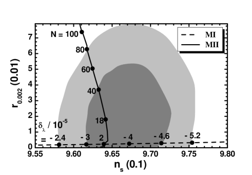
Model:	MI	MII
${\delta_{\lambda}/10^{-5}}$	$-4$	$-$
$N$	$2$	$18$
$\phi_{\star}/0.1$	$9.9564$	$9.6322$
$\Delta_{\rm\star}(\%)$	$0.44$	$3.7$
$\phi_{\rm f}/0.1$	$7.1$	$4.3$
$\lambda/10^{-5}$	$3.8$	$10.7$
$M/10^{-3}$	$5.87$	$1.96$
$n_{\rm s}/0.1$	$9.67$	$9.64$
$-\alpha_{\rm s}/10^{-4}$	$7.1$	$6.4$
$r/10^{-2}$	$0.28$	$2$

Figure 1: Allowed curves in the $n_{\rm s}-r_{0.002}$ plane fixing $M_{BL}=M_{\rm GUT}$ for MI and various $\delta_{\lambda}$’s indicated on the dashed line or MII and various $N$’s indicated on the solid line. The marginalized joint $68\%$ [$95\%$] c.l. regions from Planck TT, TE, EE+lowE+lensing, BK14 and BAO data [18] are depicted by the dark [light] shaded contours. The relevant field values, parameters and observables corresponding to $\delta_{\lambda}=-4\cdot 10^{-5}$ for MI and $N=18$ for MII are listed in the Table.

As already anticipated in both models $\phi_{\star}\sim 1$ and so a tuning emerges which can be qualified by computing $\Delta_{\rm\star}={1-\phi_{\star}}$. For MI $\Delta_{\rm\star}$ is close to $0.4\%$ and the whole observationally favored range can be covered for $\delta_{\lambda}$’s close to $10^{-5}$ whereas $r$ remaining below $0.01$. I.e.,

$$2.4\lesssim\frac{-\delta_{\lambda}}{10^{-5}}\lesssim 5.2,\>\>\>4.6\gtrsim\frac{\Delta_{\rm\star}}{10^{-3}}\gtrsim 4.1,\>\>\>5.4\lesssim\frac{-\alpha_{\rm s}}{10^{-4}}\lesssim 8.6\>\>\>\mbox{and}\>\>\>2.1\lesssim\frac{r}{10^{-3}}\lesssim 3.4\,.$$ (43)

Fixing $n_{\rm s}=0.967$ we find $\delta_{\lambda}=10^{-5}$ and $r=0.0028$. For MII $n_{\rm s}$ is concentrated a little lower than its central value and $r$ increases with $N$ and $\Delta_{\rm\star}$. I.e,

$$0.962\lesssim n_{\rm s}\lesssim 0.964,\>\>\>0.5\lesssim N\lesssim 80,\>\>\>0.45\lesssim{\Delta_{\rm\star}}/{10^{-2}}\lesssim 13.6\>\>\>\mbox{and}\>\>\>0.0025\lesssim{r}\lesssim 0.07\,.$$ (44)

We find a robust upper bound on $N$, $N\lesssim 80$, derived by the one in Eq. (7c).

The mass of the inflaton at the SUSY vacuum of Eq. (22) is given by

$$\widehat{m}_{\rm\delta\phi}=\left\langle\widehat{V}_{\rm HI,\widehat{\phi}\widehat{\phi}}\right\rangle^{1/2}=\left\langle\widehat{V}_{\rm HI,\phi\phi}/J^{2}\right\rangle^{1/2}\simeq\frac{\lambda M}{2\sqrt{N}}\cdot\begin{cases}\sqrt{1-3M^{2}}\simeq(1.7-2.1)\cdot 10^{11}~{}{\mbox{\rm GeV}}&\mbox{for {MI},}\\ \langle{f_{\rm P}}\rangle~{}~{}~{}~{}~{}\simeq(1.8-1.9)\cdot 10^{11}~{}{\mbox{\rm GeV}}&\mbox{for {MII}.}\end{cases}$$ (45)

These ranges let open the possibility of non-thermal leptogenesis [11], if we introduce a suitable coupling between the $\bar{\Phi}$ and the right-handed neutrinos $N^{c}_{i}$, $\bar{\Phi}N_{i}^{c2}$ – cf. Ref. [7, 5, 6].

4 Conclusions

We presented two models (MI and MII) of HI within SUGRA employing Kähler potentials which parameterize the $SU(2,1)/(SU(2)\times U(1))$ Kähler manifold. The Higgs fields implement the breaking of a gauge $U(1)_{B-L}$ symmetry at a scale $M$ which may assume a value compatible with the MSSM unification. Both models display a kinetic mixing with a pole of order two in the inflaton sector and respect an $R$ and the gauge symmetries. Within MI we employ $K={K_{221}}$ in Eq. (24a) and the first allowed non-renormalizable term in $W$ of Eq. (19). Any observationally acceptable $n_{\rm s}$ is attainable by tuning $\delta_{\lambda}\simeq 10^{-5}$, whereas $r\sim 10^{-3}$. Within MII we use $K={\widetilde{K}_{221}}$ in Eq. (24b) and only renormalizable terms in $W$ of Eq. (19). We find $n_{\rm s}\simeq 0.961-0.963$ and $r$ increases with $N$, which is related to ${\cal R}_{21}=-6/N$, and is bounded from above, $N\leq 80$. The inflaton mass is collectively confined into the range $(1.7-2.1)\cdot 10^{11}~{}{\mbox{\rm GeV}}$.

Work supported by the Hellenic Foundation for Research and Innovation (H.F.R.I.) under the “First Call for H.F.R.I. Research Projects to support Faculty members and Researchers and the procurement of high-cost research equipment grant” (Project Number: 2251).

References

References

- [1] J. Martin, C. Ringeval and V. Vennin, Phys. Dark Univ. 5, 75 (2014) [arXiv:1303.3787].
-
[2]
D.S. Salopek, J.R. Bond and J.M. Bardeen,
Phys. Rev. D 40, 1753 (1989);
J.L. Cervantes-Cota and H. Dehnen, Phys. Rev. D 51, 395 (1995) [astro-ph/9412032]. -
[3]
J.L. Cervantes-Cota and H. Dehnen,
Nucl. Phys. B442, 391 (1995) [astro-ph/9505069];
F.L. Bezrukov and M. Shaposhnikov, Phys. Lett. B 659, 703 (2008) [arXiv:0710.3755]. - [4] C. Pallis and N. Toumbas, J. Cosmology Astropart. Phys122011002 [arXiv:1108.1771].
-
[5]
C. Pallis,
Eur. Phys. J. C 78, no.12, 1014 (2018)
[arXiv:1807.01154];
C. Pallis, Phys. Lett. B 789, 243 (2019) [arXiv:1809.10667]. - [6] C. Pallis and Q. Shafi, Eur. Phys. J. C 78, no.6, 523 (2018) [arXiv:1803.00349].
- [7] C. Pallis, Universe 4, no.1, 13 (2018) [arXiv:1710.05759].
- [8] G. Lazarides and C. Pallis, J. High Energy Phys. 11, 114 (2015) [arXiv:1508.06682].
-
[9]
C. Pallis, Phys. Rev. D 92, no. 12, 121305(R)
(2015) [arXiv:1511.01456];
C. Pallis, J. Cosmol. Astropart. Phys. 10, no. 10, 037 (2016) [arXiv:1606.09607]. - [10] C. Pallis, J. Cosmology Astropart. Phys052021043 [arXiv:2103.05534].
-
[11]
G. Lazarides and Q. Shafi, Phys. Lett. B 258, 305 (1991);
K. Kumekawa, T. Moroi and T. Yanagida, Prog. Theor. Phys. 92, 437 (1994) [hep-ph/9405337]. - [12] N. Kaloper, L. Sorbo and J. Yokoyama, Phys. Rev. D 78, 043527 (2008) [arXiv:0803.3809].
- [13] M. Galante et al., Phys. Rev. Lett. 114, no. 14, 141302 (2015) [arXiv:1412.3797].
- [14] R. Kallosh and A. Linde, J. Cosmology Astropart. Phys072013002 [arXiv:1306.5220].
-
[15]
T. Terada, Phys. Lett. B 760, 674 (2016)
[arXiv:1602.07867];
B.J. Broy et al., J. High Energy Phys. 12, 149 (2015) [arXiv:1507.02277];
K. Nakayama et al., J. High Energy Phys. 05, 067 (2016) [arXiv:1603.02557];
T. Kobayashi, O. Seto and T.H. Tatsuishi, Prog. Theor. Phys. 123B04, no.12 (2017) [arXiv:1703.09960];
S. Karamitsos, J. Cosmology Astropart. Phys092019022 [arXiv:1903.03707]. - [16] C. Pallis, Phys. Lett. B 692, 287 (2010) [arXiv:1002.4765].
- [17] N. Aghanim et al. [Planck Collaboration], Astron. Astrophys. 641, A6 (2020) [arXiv:1807.06209].
- [18] Y. Akrami et al. [Planck Collaboration], Astron. Astrophys. 641, A10 (2020) [arXiv:1807.06211].
- [19] P. Ade et al. [BICEP2/Keck Array Collaborations], Phys.Rev.Lett. 116, 031302 (2016) [arXiv:1510.09217].
-
[20]
J.L.F. Barbon and J.R. Espinosa,
Phys. Rev. D 79, 081302 (2009) [arXiv:0903.0355];
C.P. Burgess, H.M. Lee, and M. Trott, J. High Energy Phys. 07, 007 (2010) [arXiv:1002.2730]. - [21] J.J.M. Carrasco et al., Phys. Rev. D 92, no. 4, 041301 (2015) [arXiv:1504.05557].
- [22] R. Jeannerot, S. Khalil, G. Lazarides and Q. Shafi, J. High Energy Phys. 10, 012 (2000) [hep-ph/0002151].
- [23] C. Pallis and N. Toumbas, J. Cosmology Astropart. Phys052016no. 05, 015 [arXiv:1512.05657].
- [24] G. Khanna, S. Mukhopadhyay, R. Simon and N. Mukunda, Ann. Phys. (NY) 253, 55 (1997).
-
[25]
J. Ellis, D.V. Nanopoulos and K.A. Olive,
Phys. Rev. Lett. 111, 111301 (2013);
Erratum-ibid. 111, no. 12, 129902 (2013) [arXiv:1305.1247].