Deep-Unfolding Neural-Network Aided Hybrid Beamforming Based on Symbol-Error Probability Minimization

Shuhan Shi, Yunlong Cai, Qiyu Hu, Benoit Champagne, and Lajos Hanzo S. Shi, Y. Cai, and Q. Hu are with the College of Information Science and Electronic Engineering, Zhejiang University, China (e-mail: ssh16@zju.edu.cn; ylcai@zju.edu.cn; qiyhu@zju.edu.cn). B. Champagne is with the Department of Electrical and Computer Engineering, McGill University, Canada (e-mail: benoit.champagne@mcgill.ca). L. Hanzo is with the Department of Electronics and Computer Science, University of Southampton, U.K. (e-mail: lh@ecs.soton.ac.uk).
Abstract

In massive multiple-input multiple-output (MIMO) systems, hybrid analog-digital (AD) beamforming can be used to attain a high directional gain without requiring a dedicated radio frequency (RF) chain for each antenna element, which substantially reduces both the hardware costs and power consumption. While massive MIMO transceiver design typically relies on the conventional mean-square error (MSE) criterion, directly minimizing the symbol error rate (SER) can lead to a superior performance. In this paper, we first mathematically formulate the problem of hybrid transceiver design under the minimum SER (MSER) optimization criterion and then develop a MSER-based gradient descent (GD) iterative algorithm to find the related stationary points. We then propose a deep-unfolding neural network (NN), in which the iterative GD algorithm is unfolded into a multi-layer structure wherein a set of trainable parameters are introduced for accelerating the convergence and enhancing the overall system performance. To implement the training stage, the relationship between the gradients of adjacent layers is derived based on the generalized chain rule (GCR). The deep-unfolding NN is developed for both quadrature phase shift keying (QPSK) and for M๐‘€M-ary quadrature amplitude modulated (QAM) signals and its convergence is investigated theoretically. Furthermore, we analyze the transfer capability, computational complexity, and generalization capability of the proposed deep-unfolding NN. Our simulation results show that the latter significantly outperforms its conventional counterpart at a reduced complexity.

Index Terms:
Hybrid beamforming, massive MIMO, deep-unfolding, MSER, machine learning.

I Introduction

The massive multiple-input multiple-output (MIMO) technology has inspired wide research-attention, since it is capable of dramatically increasing the system capacity, hence mitigating the spectrum shortage [1, 2, 3]. This is achieved by forming directional beams. However, these large-scale antenna arrays employed both at the transmitter and receiver have a prohibitive hardware cost and power consumption in fully-digital (FD) beamforming, where each antenna element requires a dedicated radio frequency (RF) chain. Thus, hybrid analog-digital (AD) beamforming has become an important technique of reducing the number of RF chains, while still approaching the performance of fully-digital beamforming [3, 4, 5, 6, 7, 8, 10, 9, 11, 12, 13, 14].

I-A Prior Art

Hybrid AD beamforming conceptually relies on the decomposition of the beamforming operation as the product of a low-dimensional digital beamforming matrix and a high-dimensional analog beamforming matrix. The elements of the analog beamforming matrix obey the unit-modulus constraint imposed by the phase shifters. To reduce the number of RF chains, several authorsย [4, 5] advocated antenna-selection based hybrid beamforming. In order to further improve their performance, spatially sparse precoding techniques were developed by exploiting the millimeter-wave (mmWave) channel characteristics in [3, 6]. Moreover, the authors ofย [7] demonstrated that hybrid AD beamforming having twice as many RF chains as data streams approaches the performance of FD beamforming.

Inspired by these findings, sophisticated optimization algorithms were proposed for hybrid beamformingย [6, 8, 10, 9, 11, 12, 13, 14]. In [6], the authors leveraged the channelโ€™s sparsity and proposed an orthogonal matching pursuit (OMP) aided algorithm. Based on the OMP concept, the authors of ย [8, 10, 9] developed a hybrid transceiver architecture relying on the minimum mean square error (MMSE) criterion. Inย [11], the authors formulated a matrix factorization problem and developed a manifold optimization (MO) based hybrid beamforming algorithm, where the unit-modulus constraint was considered as a Riemannian manifold. Inย [12], a codebook-based hybrid beamforming design was conceived for maximizing the systemโ€™s spectral efficiency. As a further development, the authors ofย [13] conceived a two-stage optimization algorithm based on the general eigen-decomposition method and their work evolved further inย [14] to the broadband scenario with the aid of MO.

However, most of the existing hybrid beamforming designs in the open literature are based on the minimization of the mean square error (MSE), which is not the most appropriate metric from a performance viewpoint in digital communications where the standard measure is the symbol-error-rate (SER). Recently, a number of powerful beamformers have been designed based on the minimum SER (MSER) criterionย [15, 16, 17, 18, 19]. The authors of [15] and [16] developed a MSER-based adaptive reduced-rank receive beamformer for enhancing the performance. Inย [17], a single-bit direct MSER-optimization based precoder was proposed for simplifying the RF chains. The authors ofย [18] designed an interference-aided precoder for minimizing the SER of the worst-case user in the system. As a further development, inย [19], the authors proposed a MSER-based precoder for K๐พK-pair MIMO interference channels by utilizing improper signaling. However, due to the associated complex high-dimensional matrix inversions and decompositions, the existing optimization algorithms suffer from high complexity in practical implementation.

To improve the performance at a reduced complexity, researchers have recently turned their attention to machine learning techniques for solving a variety of problems, such as channel decodingย [20], end-to-end communicationย [21, 22], and channel estimationย [23]. Well-trained neural networks (NNs) are capable of learning the mapping between the system inputs and outputsย [24, 25, 26, 27, 28, 29]. One of the early attempts along this avenue appeared inย [24], where a NN was trained for performing power allocation based on an iterative weighted MMSE (WMMSE) algorithm. The authors ofย [25] proposed a two-stage training mechanism for maximizing the sum-rate by applying convolutional neural networks (CNN), and further improved the system performance through unsupervised learning. Inย [26], the authors adopted an ensemble of fully connected deep neural networks (DNNs) for optimizing the transmit power allocation. Inย [27], the problem of joint antenna selection and hybrid beamforming was first formulated as a classification problem, and then solved by a deep CNN. Deep learning was also utilized for jointly optimizing the compressive channel and hybrid beamforming matrices inย [28]. In [29], the authors designed a novel NN inspired by GoogleNet, which used parallel complex convolutional blocks for hybrid beamforming.

In the above contributions, NNs are generally treated as black-boxes, which does not guarantee optimal performance and leads to limited interpretability, along with limited control. Furthermore, in massive MIMO systems, the training overhead of these methods is expensive due to the multi-dimensional training samples and long training time. To overcome these issues, a model-driven network, which is referred to as deep-unfolding, has been proposed inย [30]. This method generally unfolds iterative algorithms into multi-layer NN structures and introduces a set of trainable parameters to accelerate convergence and to increase the system performance. The authors ofย [31] and [32] invoked this approach to unfold the gradient descent (GD) algorithm for data detection. Inย [33, 34] the authors developed a deep-unfolding method inspired by the normalized min-sum algorithm for the decoding of polar codes. Inย [35], a scheme based on deep-unfolding was put forward for sparse signal recovery. In [36], the authors employed the deep-unfolding method for automatically optimizing the precoders relying on single-bit digital-to-analog converters (DACs). The authors of [37] adopted a deep-unfolding NN based on the conjugate GD algorithm for constant envelope precoding. A finite-alphabet precoder was developed in [38], which unfolded the iterative discrete estimation algorithm into a NN. In [39], the authors derived the generalized chain rule (GCR) in matrix form and proposed a deep-unfolding NN based on the WMMSE precoding design algorithm.

I-B Main Contributions

The MSER-based hybrid beamforming design problem in massive MIMO systems is very challenging due to the highly nonconvex objective function and unit-modulus constraints. While the GD algorithm is a common technique that can be adopted for finding the stationary points, it requires a long time to converge and a large number of iterations. Since the deep-unfolding method makes full use of the structure of the iterative algorithm and only replaces some complex operations with trainable parameters, it can significantly reduce the computational complexity with only a slight performance loss. To the best of our knowledge however, the deep-unfolding method has not been investigated in the context of hybrid beamforming based on the MSER criterion. Hence we first mathematically formulate the problem of hybrid AD transceiver design under the direct MSER criterion in a hardware-efficient massive MIMO system. We then develop a MSER-based GD iterative algorithm for finding the stationary points. Specifically, we propose a deep-unfolding NN, in which the iterative GD algorithm is unfolded into a multi-layer structure and then a set of trainable parameters are introduced into the forward propagation (FP) for accelerating the convergence and enhancing the system performance. In the training stage, the relationship between the gradients of adjacent layers is derived based on the GCR in the back propagation (BP). Then a deep-unfolding NN is developed for both quadrature phase shift keying (QPSK) and M๐‘€M-ary quadrature amplitude modulation (QAM) signals. While deep-unfolding NNs often lack solid theoretical support, we herein provide a detailed theoretical convergence analysis of the proposed schemes. As a benchmark, we develop a deep learning aided black-box based CNN for hybrid transceiver design. Furthermore, we analyze the transfer ability, computational complexity and generalization capability of the proposed deep-unfolding NN. Our simulation results show that the proposed deep-unfolding NN significantly outperforms the conventional algorithms and approaches the performance of the MSER-based GD iterative algorithm at a much reduced complexity. The main contributions of this work are summarized as follows:

  • โ€ข

    We formulate the joint hybrid AD transceiver design problem based on the MSER criterion in a massive MIMO system context, which is very challenging to tackle due to the highly nonconvex objective function and unit-modulus constraints imposed on the entries of the analog beamforming matrix. Then an unconstrained MSER-based GD iterative algorithm is developed for finding the stationary points through the application of kernel density estimation and a parametric representation of the unit-modulus matrix entries.

  • โ€ข

    We propose a deep-unfolding NN based on the MSER-based GD iterative algorithm to expedite convergence while guaranteeing the performance of our hybrid transceiver design, wherein the iterative algorithm is unfolded into a multi-layer structure and a set of trainable parameters are introduced.

  • โ€ข

    We provide a theoretical analysis for the convergence of the proposed deep-unfolding NNs and also analyze their transfer ability, computational complexity and generalization capability.

  • โ€ข

    Through numerical simulation, we show that the proposed deep-unfolding NN substantially outperforms the conventional black-box method and approaches the performance of the MSER-based GD algorithm at a significantly reduced number of iterations, which translates into reduced complexity.

I-C Organization

The paper is structured as follows. Section II briefly describes the system model. Section III formulates the MSER-based hybrid transceiver design problem for the case of QPSK and develops a MSER-based GD algorithm. The deep-unfolding NN is conceived in Section IV. In Section V, a black-box NN as a benchmark, the analysis of the computational complexity and generalization ability and the extension of the proposed algorithm to the QAM modulation are provided. The simulation results are presented in Section VI and conclusions are drawn in Section VII.

Notations: Scalars, vectors and matrices are respectively denoted by lower case, boldface lower case and boldface upper case letters. ๐ˆ๐ˆ\mathbf{I} represents an identity matrix and ๐ŸŽ0\mathbf{0} denotes an all-zero matrix. For a matrix ๐€๐€\mathbf{A}, ๐€Tsuperscript๐€๐‘‡{{\bf{A}}^{T}}, ๐€โˆ—superscript๐€\mathbf{A}^{*}, ๐€Hsuperscript๐€๐ป{{\bf{A}}^{H}}, ๐€โŸ‚superscript๐€perpendicular-to\mathbf{A}^{\perp}, โ€–๐€โ€–norm๐€\|\mathbf{A}\| and [๐€]m,nsubscriptdelimited-[]๐€๐‘š๐‘›[\mathbf{A}]_{m,n} denote its transpose, conjugate, conjugate transpose, reciprocal by element, Frobenius norm and element at the intersection of row m๐‘šm and column n๐‘›n, respectively. For a vector ๐š๐š\mathbf{a}, โ€–๐šโ€–norm๐š\|\mathbf{a}\| represents its Euclidean norm. ๐”ผ{.}\mathbb{E}\{.\} denotes the statistical expectation. โ„œ{.}\Re\{.\} (โ„‘{.}\Im\{.\}) denotes the real (imaginary) part of a variable. The operator vecโ€‹(โ‹…)vecโ‹…\textrm{vec}(\cdot) stacks the columns of a matrix in one long column vector. |โ‹…||\cdot| denotes the absolute value of a complex scalar. โ„‚mร—nโ€‹(โ„mร—n)superscriptโ„‚๐‘š๐‘›superscriptโ„๐‘š๐‘›{\mathbb{C}^{m\times n}}\;({\mathbb{R}^{m\times n}}) denotes the space of mร—n๐‘š๐‘›{m\times n} complex (real) matrices. The operator โˆ โˆ \angle takes the phase angles of the elements in a matrix. The symbol โˆ˜\circ denotes the Hadamard product of two vectors/matrices.

II System Model
Refer to caption
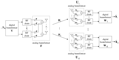
Figure 1: Hardware-efficient massive MIMO system for downlink transmission.

We consider the downlink of a hardware-efficient massive MIMO system as depicted in Fig. 1, which consists of one base station (BS) and K๐พK users. The BS is equipped with Ntsubscript๐‘๐‘กN_{t} transmit antennas and Rtโ€‹(Rtโ‰ชNt)subscript๐‘…๐‘กmuch-less-thansubscript๐‘…๐‘กsubscript๐‘๐‘กR_{t}(R_{t}\ll N_{t}) RF chains. User kโˆˆ๐’ฆโ‰œ{1,โ€ฆ,K}๐‘˜๐’ฆโ‰œ1โ€ฆ๐พk\in\mathcal{K}\triangleq\{1,\ldots,K\} is equipped with Nr,ksubscript๐‘๐‘Ÿ๐‘˜N_{r,k} receive antennas and Rr,kโ€‹(Rr,kโ‰คNr,k)subscript๐‘…๐‘Ÿ๐‘˜subscript๐‘…๐‘Ÿ๐‘˜subscript๐‘๐‘Ÿ๐‘˜R_{r,k}(R_{r,k}\leq N_{r,k}) RF chains, where Ntโ‰ซโˆ‘k=1KNr,kmuch-greater-thansubscript๐‘๐‘กsubscriptsuperscript๐พ๐‘˜1subscript๐‘๐‘Ÿ๐‘˜N_{t}\gg\sum^{K}_{k=1}N_{r,k} and Rtโ‰ฅโˆ‘k=1KRr,ksubscript๐‘…๐‘กsubscriptsuperscript๐พ๐‘˜1subscript๐‘…๐‘Ÿ๐‘˜R_{t}\geq\sum^{K}_{k=1}R_{r,k}. The BS transmits a symbol vector ๐ฌโ‰œ[๐›1T,๐›2T,โ€ฆ,๐›KT]Tโˆˆโ„‚Dร—1โ‰œ๐ฌsuperscriptsuperscriptsubscript๐›1๐‘‡superscriptsubscript๐›2๐‘‡โ€ฆsuperscriptsubscript๐›๐พ๐‘‡๐‘‡superscriptโ„‚๐ท1\mathbf{s}\triangleq[\mathbf{b}_{1}^{T},\mathbf{b}_{2}^{T},\ldots,\mathbf{b}_{K}^{T}]^{T}\in\mathbb{C}^{D\times 1} to the users, where the transmit symbols are independent and identically distributed (i.i.d.). The symbol vector of user kโˆˆ๐’ฆ๐‘˜๐’ฆk\in\mathcal{K}, ๐›kโ‰œ[b1,k,โ€ฆ,bDk,k]Tโˆˆโ„‚Dkร—1โ‰œsubscript๐›๐‘˜superscriptsubscript๐‘1๐‘˜โ€ฆsubscript๐‘subscript๐ท๐‘˜๐‘˜๐‘‡superscriptโ„‚subscript๐ท๐‘˜1\mathbf{b}_{k}\triangleq[b_{1,k},\ldots,b_{D_{k},k}]^{T}\in\mathbb{C}^{D_{k}\times 1}, has zero-mean and covariance matrix ๐”ผโ€‹[๐›kโ€‹๐›kH]=๐ˆ๐”ผdelimited-[]subscript๐›๐‘˜superscriptsubscript๐›๐‘˜๐ป๐ˆ\mathbb{E}[\mathbf{b}_{k}\mathbf{b}_{k}^{H}]=\mathbf{I}, where Dksubscript๐ท๐‘˜D_{k} (Dkโ‰คRr,ksubscript๐ท๐‘˜subscript๐‘…๐‘Ÿ๐‘˜D_{k}\leq R_{r,k}) denotes the number of data streams for user k๐‘˜k, and D=โˆ‘k=1KDk๐ทsuperscriptsubscript๐‘˜1๐พsubscript๐ท๐‘˜D=\sum\limits_{k=1}^{K}D_{k} denotes the total number of data streams. In this work, QPSK and M๐‘€M-ary square QAM symbol constellations are adopted, although extensions to other types of constellations are possible. For the QPSK case, the real and imaginary parts of each entry of the signal vector ๐›ksubscript๐›๐‘˜\mathbf{b}_{k} are uniformly drawn from {ยฑ1}plus-or-minus1\{\pm 1\}. For the M๐‘€M-QAM modulation, each entry of ๐›ksubscript๐›๐‘˜\mathbf{b}_{k} is uniformly drawn from {Fm+jโ€‹Fn:1โ‰คm,nโ‰คM}conditional-setsubscript๐น๐‘š๐‘—subscript๐น๐‘›formulae-sequence1๐‘š๐‘›๐‘€\{F_{m}+jF_{n}:1\leq m,n\leq\sqrt{M}\}, where integer M๐‘€M is a perfect square and we define Fn=2โ€‹nโˆ’Mโˆ’1subscript๐น๐‘›2๐‘›๐‘€1F_{n}=2n-\sqrt{M}-1. The transmitted symbol vector ๐ฌ๐ฌ\mathbf{s} is first processed by a digital transmit beamforming matrix ๐•โ‰œ[๐1,โ€ฆ,๐K]โˆˆโ„‚Rtร—Dโ‰œ๐•subscript๐1โ€ฆsubscript๐๐พsuperscriptโ„‚subscript๐‘…๐‘ก๐ท\mathbf{V}\triangleq[\mathbf{P}_{1},\ldots,\mathbf{P}_{K}]\in\mathbb{C}^{R_{t}\times D}, where ๐kโˆˆโ„‚Rtร—Dksubscript๐๐‘˜superscriptโ„‚subscript๐‘…๐‘กsubscript๐ท๐‘˜\mathbf{P}_{k}\in\mathbb{C}^{R_{t}\times D_{k}} denotes the transmit beamforming matrix for user k๐‘˜k. The digital beamformer output is passed through the RF chains and then processed by an analog transmit beamforming matrix ๐…โˆˆโ„‚Ntร—Rt๐…superscriptโ„‚subscript๐‘๐‘กsubscript๐‘…๐‘ก\mathbf{F}\in\mathbb{C}^{N_{t}\times R_{t}} implemented by means of phase shifters, i.e., |[๐…]m,n|=1subscriptdelimited-[]๐…๐‘š๐‘›1|[\mathbf{F}]_{m,n}|=1. The transmit power constraint at the BS is given by

๐”ผโ€‹{โ€–๐…๐•๐ฌโ€–2}=โ€–๐…๐•โ€–2=PT,๐”ผsuperscriptnorm๐…๐•๐ฌ2superscriptnorm๐…๐•2subscript๐‘ƒ๐‘‡\mathbb{E}\{\|\mathbf{F}\mathbf{V}\mathbf{s}\|^{2}\}=\|\mathbf{F}\mathbf{V}\|^{2}=P_{T},\vspace{-1mm} (1)

where PTsubscript๐‘ƒ๐‘‡P_{T} denotes the total transmit power budget.

The signal received at user k๐‘˜k is given by

๐ฒk=๐‡kโ€‹๐…๐•๐ฌ+๐งk=๐‡kโ€‹๐…โ€‹โˆ‘k=1K๐kโ€‹๐›k+๐งk,subscript๐ฒ๐‘˜subscript๐‡๐‘˜๐…๐•๐ฌsubscript๐ง๐‘˜subscript๐‡๐‘˜๐…subscriptsuperscript๐พ๐‘˜1subscript๐๐‘˜subscript๐›๐‘˜subscript๐ง๐‘˜\mathbf{y}_{k}=\mathbf{H}_{k}\mathbf{F}\mathbf{V}\mathbf{s}+\mathbf{n}_{k}=\mathbf{H}_{k}\mathbf{F}\sum^{K}_{k=1}\mathbf{P}_{k}\mathbf{b}_{k}+\mathbf{n}_{k},\vspace{-2mm} (2)

where ๐‡kโˆˆโ„‚Nr,kร—Ntsubscript๐‡๐‘˜superscriptโ„‚subscript๐‘๐‘Ÿ๐‘˜subscript๐‘๐‘ก\mathbf{H}_{k}\in\mathbb{C}^{N_{r,k}\times N_{t}} denotes the massive MIMO channel matrix between the BS and user k๐‘˜k. As discussed in [6] and [7], this matrix is conveniently described by a geometry clustered channel model with NCsubscript๐‘๐ถN_{C} clusters and NRsubscript๐‘๐‘…N_{R} rays in each cluster due to the sparse scattering property of massive MIMO channels. Considering a system with a half-wave spaced uniform linear array at both the transmitter and the receiver, we have without loss of generality

๐‡k=Ntโ€‹Nr,kNCโ€‹NRโ€‹โˆ‘i=1NCโˆ‘j=1NRฮฑi,jโ€‹๐šrโ€‹(ฮธi,jr)โ€‹๐štโ€‹(ฮธi,jt)H,subscript๐‡๐‘˜subscript๐‘๐‘กsubscript๐‘๐‘Ÿ๐‘˜subscript๐‘๐ถsubscript๐‘๐‘…superscriptsubscript๐‘–1subscript๐‘๐ถsuperscriptsubscript๐‘—1subscript๐‘๐‘…subscript๐›ผ๐‘–๐‘—subscript๐š๐‘Ÿsuperscriptsubscript๐œƒ๐‘–๐‘—๐‘Ÿsubscript๐š๐‘กsuperscriptsuperscriptsubscript๐œƒ๐‘–๐‘—๐‘ก๐ป\mathbf{H}_{k}=\sqrt{\dfrac{N_{t}N_{r,k}}{N_{C}N_{R}}}\sum_{i=1}^{N_{C}}\sum_{j=1}^{N_{R}}\alpha_{i,j}\mathbf{a}_{r}(\theta_{i,j}^{r})\mathbf{a}_{t}(\theta_{i,j}^{t})^{H},\vspace{-1mm} (3)

where ฮฑi,jsubscript๐›ผ๐‘–๐‘—\alpha_{i,j} denotes the complex propagation gain of the j๐‘—j-th ray in the i๐‘–ith cluster, while ๐šrโ€‹(ฮธi,jr)โ‰œ1Nr,kโ€‹[1,ejโ€‹ฯ€โ€‹sโ€‹iโ€‹nโ€‹ฮธi,jr,โ€ฆ,ejโ€‹ฯ€โ€‹(Nrโˆ’1)โ€‹sโ€‹iโ€‹nโ€‹ฮธi,jr]Tโ‰œsubscript๐š๐‘Ÿsuperscriptsubscript๐œƒ๐‘–๐‘—๐‘Ÿ1subscript๐‘๐‘Ÿ๐‘˜superscript1superscript๐‘’๐‘—๐œ‹๐‘ ๐‘–๐‘›superscriptsubscript๐œƒ๐‘–๐‘—๐‘Ÿโ€ฆsuperscript๐‘’๐‘—๐œ‹subscript๐‘๐‘Ÿ1๐‘ ๐‘–๐‘›superscriptsubscript๐œƒ๐‘–๐‘—๐‘Ÿ๐‘‡\mathbf{a}_{r}(\theta_{i,j}^{r})\triangleq\dfrac{1}{\sqrt{N_{r,k}}}[1,e^{j\pi sin\theta_{i,j}^{r}},\ldots,e^{j\pi(N_{r}-1)sin\theta_{i,j}^{r}}]^{T} and ๐štโ€‹(ฮธi,jt)โ‰œ1Ntโ€‹[1,ejโ€‹ฯ€โ€‹sโ€‹iโ€‹nโ€‹ฮธi,jt,โ€ฆ,ejโ€‹ฯ€โ€‹(Ntโˆ’1)โ€‹sโ€‹iโ€‹nโ€‹ฮธi,jt]Tโ‰œsubscript๐š๐‘กsuperscriptsubscript๐œƒ๐‘–๐‘—๐‘ก1subscript๐‘๐‘กsuperscript1superscript๐‘’๐‘—๐œ‹๐‘ ๐‘–๐‘›superscriptsubscript๐œƒ๐‘–๐‘—๐‘กโ€ฆsuperscript๐‘’๐‘—๐œ‹subscript๐‘๐‘ก1๐‘ ๐‘–๐‘›superscriptsubscript๐œƒ๐‘–๐‘—๐‘ก๐‘‡\mathbf{a}_{t}(\theta_{i,j}^{t})\triangleq\dfrac{1}{\sqrt{N_{t}}}[1,e^{j\pi sin\theta_{i,j}^{t}},\ldots,e^{j\pi(N_{t}-1)sin\theta_{i,j}^{t}}]^{T} denote the corresponding normalized response vectors of the transmit and receive antenna arrays, with ฮธi,jrsubscriptsuperscript๐œƒ๐‘Ÿ๐‘–๐‘—\theta^{r}_{i,j} and ฮธi,jtsubscriptsuperscript๐œƒ๐‘ก๐‘–๐‘—\theta^{t}_{i,j} denoting the angles of arrival and departure, respectively. The term ๐งkโˆˆโ„‚Nr,kร—1subscript๐ง๐‘˜superscriptโ„‚subscript๐‘๐‘Ÿ๐‘˜1\mathbf{n}_{k}\in\mathbb{C}^{N_{r,k}\times 1} in (2) represents the additive noise at user k๐‘˜k, modeled as a complex circularly symmetric Gaussian vector with zero-mean and covariance matrix ๐”ผโ€‹[๐งkโ€‹๐งkH]=ฯƒk2โ€‹๐ˆ๐”ผdelimited-[]subscript๐ง๐‘˜superscriptsubscript๐ง๐‘˜๐ปsuperscriptsubscript๐œŽ๐‘˜2๐ˆ\mathbb{E}[\mathbf{n}_{k}\mathbf{n}_{k}^{H}]=\sigma_{k}^{2}\mathbf{I}.

Similar to the BS, the hybrid AD receiver at user k๐‘˜k is comprised of an analog receive beamforming matrix ๐”kโˆˆโ„‚Rr,kร—Nrsubscript๐”๐‘˜superscriptโ„‚subscript๐‘…๐‘Ÿ๐‘˜subscript๐‘๐‘Ÿ\mathbf{U}_{k}\in\mathbb{C}^{R_{r,k}\times N_{r}}, followed by a digital receive beamforming matrix ๐–kโ‰œ[๐ฐ1,k,โ€ฆ,๐ฐDk,k]โˆˆโ„‚Rr,kร—Dkโ‰œsubscript๐–๐‘˜subscript๐ฐ1๐‘˜โ€ฆsubscript๐ฐsubscript๐ท๐‘˜๐‘˜superscriptโ„‚subscript๐‘…๐‘Ÿ๐‘˜subscript๐ท๐‘˜\mathbf{W}_{k}\triangleq[\mathbf{w}_{1,k},\ldots,\mathbf{w}_{D_{k},k}]\in\mathbb{C}^{R_{r,k}\times D_{k}}, where ๐ฐi,kโˆˆโ„‚Rr,kร—1subscript๐ฐ๐‘–๐‘˜superscriptโ„‚subscript๐‘…๐‘Ÿ๐‘˜1\mathbf{w}_{i,k}\in\mathbb{C}^{R_{r,k}\times 1} and iโˆˆ๐’Ÿkโ‰œ{1,โ€ฆ,Dk}๐‘–subscript๐’Ÿ๐‘˜โ‰œ1โ€ฆsubscript๐ท๐‘˜i\in\mathcal{D}_{k}\triangleq\{1,\ldots,D_{k}\}. Accordingly, the output signal vector ๐›~kโ‰œ[b~1,k,โ€ฆ,b~Dk,k]Tโˆˆโ„‚Dkร—1โ‰œsubscript~๐›๐‘˜superscriptsubscript~๐‘1๐‘˜โ€ฆsubscript~๐‘subscript๐ท๐‘˜๐‘˜๐‘‡superscriptโ„‚subscript๐ท๐‘˜1\tilde{\mathbf{b}}_{k}\triangleq[\tilde{b}_{1,k},\ldots,\tilde{b}_{D_{k},k}]^{T}\in\mathbb{C}^{D_{k}\times 1} of the hybrid receiver at user k๐‘˜k can be expressed as

๐›~k=๐–kHโ€‹๐”kโ€‹๐ฒk=๐–kHโ€‹๐”kโ€‹(๐‡kโ€‹๐…โ€‹โˆ‘k=1K๐kโ€‹๐›k+๐งk),subscript~๐›๐‘˜subscriptsuperscript๐–๐ป๐‘˜subscript๐”๐‘˜subscript๐ฒ๐‘˜subscriptsuperscript๐–๐ป๐‘˜subscript๐”๐‘˜subscript๐‡๐‘˜๐…subscriptsuperscript๐พ๐‘˜1subscript๐๐‘˜subscript๐›๐‘˜subscript๐ง๐‘˜\tilde{\mathbf{b}}_{k}=\mathbf{W}^{H}_{k}\mathbf{U}_{k}\mathbf{y}_{k}=\mathbf{W}^{H}_{k}\mathbf{U}_{k}(\mathbf{H}_{k}\mathbf{F}\sum^{K}_{k=1}\mathbf{P}_{k}\mathbf{b}_{k}+\mathbf{n}_{k}),\vspace{-1mm} (4)

where the entries of the analog beamforming matrices obey the unit-modulus constraints, i.e., |[๐”k]m,n|=1subscriptdelimited-[]subscript๐”๐‘˜๐‘š๐‘›1|[\mathbf{U}_{k}]_{m,n}|=1, โˆ€kโˆˆ๐’ฆfor-all๐‘˜๐’ฆ\forall k\in\mathcal{K}.

Finally, the estimate of the transmitted symbol vector ๐›ksubscript๐›๐‘˜\mathbf{b}_{k} at the output of receiver k๐‘˜k is

๐›^k=๐’ฌโ€‹{๐›~k},subscript^๐›๐‘˜๐’ฌsubscript~๐›๐‘˜\hat{\mathbf{b}}_{k}=\mathcal{Q}\{\tilde{\mathbf{b}}_{k}\},\vspace{-1mm} (5)

where ๐’ฌโ€‹{โ‹…}๐’ฌโ‹…\mathcal{Q}\{\cdot\} is the quantization operation for the given modulation.

The basic problem in implementing the hybrid AD transceiver scheme is how to effectively design the beamforming matrices {๐k,๐–k,๐”k,๐…}subscript๐๐‘˜subscript๐–๐‘˜subscript๐”๐‘˜๐…\{\mathbf{P}_{k},\mathbf{W}_{k},\mathbf{U}_{k},\mathbf{F}\} to detect the transmitted symbols accurately under the total transmit power constraint at the BS and the unit-modulus constraint imposed on each element of the analog RF beamforming matrices at the BS and user sides.

III Proposed MSER-Based GD Algorithm for Hybrid AD Transceiver Design

In this section, we focus on the QPSK case to formulate the MSER criterion mathematically. The resultant problem is very difficult to tackle due to the highly nonlinear objective function and constraints. We then develop a MSER-based GD iterative algorithm for finding the stationary points, which will serve as the basis in the elaboration of our proposed deep unfolding NN.

III-A MSER Criterion

The decisions for the detection of the real and imaginary parts of element iโˆˆ๐’Ÿk๐‘–subscript๐’Ÿ๐‘˜i\in\mathcal{D}_{k} in the k๐‘˜k-th userโ€™s symbol vector ๐›k=[b1,k,โ€ฆ,bDk,k]Tsubscript๐›๐‘˜superscriptsubscript๐‘1๐‘˜โ€ฆsubscript๐‘subscript๐ท๐‘˜๐‘˜๐‘‡\mathbf{b}_{k}=[b_{1,k},...,b_{D_{k},k}]^{T} are made as

โ„œ{b^i,k}={+1,ifโ€‹โ„œโก{b~i,k}โ‰ฅ0โˆ’1,ifโ€‹โ„œโก{b~i,k}<0,โ„‘{b^i,k}={+1,ifโ€‹โ„‘โก{b~i,k}โ‰ฅ0โˆ’1,ifโ€‹โ„‘โก{b~i,k}<0.\begin{split}\Re\{\hat{b}_{i,k}\}=\left\{\begin{aligned} &+1,\qquad\textrm{if}\ \Re\{\tilde{b}_{i,k}\}\geq 0\\ &-1,\qquad\textrm{if}\ \Re\{\tilde{b}_{i,k}\}<0,\end{aligned}\right.\\ \Im\{\hat{b}_{i,k}\}=\left\{\begin{aligned} &+1,\qquad\textrm{if}\ \Im\{\tilde{b}_{i,k}\}\geq 0\\ &-1,\qquad\textrm{if}\ \Im\{\tilde{b}_{i,k}\}<0.\vspace{-1mm}\end{aligned}\right.\end{split} (6)

For a given desired symbol bi,ksubscript๐‘๐‘–๐‘˜b_{i,k}, there exists Nb=4Dโˆ’1subscript๐‘๐‘superscript4๐ท1N_{b}=4^{D-1} legitimate combinations of the multi-user interference symbols {bi,kโ€ฒ,iโˆˆ๐’Ÿkโ€ฒ,kโ€ฒโˆˆ๐’ฆ,kโ€ฒโ‰ k}formulae-sequencesubscript๐‘๐‘–superscript๐‘˜โ€ฒ๐‘–subscript๐’Ÿsuperscript๐‘˜โ€ฒformulae-sequencesuperscript๐‘˜โ€ฒ๐’ฆsuperscript๐‘˜โ€ฒ๐‘˜\{b_{i,k^{\prime}},i\in\mathcal{D}_{k^{{}^{\prime}}},k^{\prime}\in\mathcal{K},k^{\prime}\neq k\} and self-interference symbols {biโ€ฒ,k,iโ€ฒโˆˆ๐’Ÿk,iโ€ฒโ‰ i}formulae-sequencesubscript๐‘superscript๐‘–โ€ฒ๐‘˜superscript๐‘–โ€ฒsubscript๐’Ÿ๐‘˜superscript๐‘–โ€ฒ๐‘–\{b_{i^{{}^{\prime}},k},i^{\prime}\in\mathcal{D}_{k},i^{\prime}\neq i\}. We define the set of all the possible transmitted symbol vectors as

๐’ณโ‰œ{๐ฌ1,๐ฌ2,โ€ฆ,๐ฌNb},โ‰œ๐’ณsuperscript๐ฌ1superscript๐ฌ2โ€ฆsuperscript๐ฌsubscript๐‘๐‘\mathcal{X}\triangleq\{\mathbf{s}^{1},\mathbf{s}^{2},\ldots,\mathbf{s}^{N_{b}}\}, (7)

where ๐ฌq=[(๐›1q)T,(๐›2q)T,โ€ฆ,(๐›Kq)T]Tsuperscript๐ฌ๐‘žsuperscriptsuperscriptsuperscriptsubscript๐›1๐‘ž๐‘‡superscriptsuperscriptsubscript๐›2๐‘ž๐‘‡โ€ฆsuperscriptsuperscriptsubscript๐›๐พ๐‘ž๐‘‡๐‘‡\mathbf{s}^{q}=[(\mathbf{b}_{1}^{q})^{T},(\mathbf{b}_{2}^{q})^{T},\ldots,(\mathbf{b}_{K}^{q})^{T}]^{T}, qโˆˆ๐’ฉbโ‰œ{1,โ€ฆ,Nb}๐‘žsubscript๐’ฉ๐‘โ‰œ1โ€ฆsubscript๐‘๐‘q\in\mathcal{N}_{b}\triangleq\{1,\ldots,N_{b}\}, and we assume an equiprobable model for the Nbsubscript๐‘๐‘N_{b} possible transmit vectors ๐ฌqsuperscript๐ฌ๐‘ž\mathbf{s}^{q}. The noise-free component for the i๐‘–i-th element of the hybrid receiverโ€™s output at user k๐‘˜k is from the set

๐’ดi,kโ‰œ{bยฏi,kq=๐ฐi,kHโ€‹๐”kโ€‹๐‡kโ€‹๐…๐•๐ฌq,qโˆˆ๐’ฉb}.โ‰œsubscript๐’ด๐‘–๐‘˜formulae-sequencesubscriptsuperscriptยฏ๐‘๐‘ž๐‘–๐‘˜subscriptsuperscript๐ฐ๐ป๐‘–๐‘˜subscript๐”๐‘˜subscript๐‡๐‘˜superscript๐…๐•๐ฌ๐‘ž๐‘žsubscript๐’ฉ๐‘\mathcal{Y}_{i,k}\triangleq\{\bar{b}^{q}_{i,k}=\mathbf{w}^{H}_{i,k}\mathbf{U}_{k}\mathbf{H}_{k}\mathbf{F}\mathbf{V}\mathbf{s}^{q},\,q\in\mathcal{N}_{b}\}.\vspace{-1mm} (8)

Due to the Gaussian distribution for the additive noise at the receiver, and invoking the law of total probability, we can express the probability density function (PDF) for the real part of the hybrid receiverโ€™s output, given the symbol bi,ksubscript๐‘๐‘–๐‘˜b_{i,k}, as

fโ€‹(x|bi,k)=1Nbโ€‹2โ€‹ฯ€โ€‹๐ฐi,kHโ€‹๐”kโ€‹๐‡kโ€‹๐…๐•๐•Hโ€‹๐…Hโ€‹๐‡kHโ€‹๐”kHโ€‹๐ฐi,kโ€‹ฯƒnโˆ‘q=1Nbeโˆ’|xโˆ’โ„œโก{bยฏi,kq}|22โ€‹๐ฐi,kHโ€‹๐”kโ€‹๐‡kโ€‹๐…๐•๐•Hโ€‹๐…Hโ€‹๐‡kHโ€‹๐”kHโ€‹๐ฐi,kโ€‹ฯƒn2,๐‘“conditional๐‘ฅsubscript๐‘๐‘–๐‘˜1subscript๐‘๐‘2๐œ‹superscriptsubscript๐ฐ๐‘–๐‘˜๐ปsubscript๐”๐‘˜subscript๐‡๐‘˜superscript๐…๐•๐•๐ปsuperscript๐…๐ปsuperscriptsubscript๐‡๐‘˜๐ปsuperscriptsubscript๐”๐‘˜๐ปsubscript๐ฐ๐‘–๐‘˜subscript๐œŽ๐‘›superscriptsubscript๐‘ž1subscript๐‘๐‘superscript๐‘’superscript๐‘ฅsubscriptsuperscriptยฏ๐‘๐‘ž๐‘–๐‘˜22subscriptsuperscript๐ฐ๐ป๐‘–๐‘˜subscript๐”๐‘˜subscript๐‡๐‘˜superscript๐…๐•๐•๐ปsuperscript๐…๐ปsuperscriptsubscript๐‡๐‘˜๐ปsuperscriptsubscript๐”๐‘˜๐ปsubscript๐ฐ๐‘–๐‘˜superscriptsubscript๐œŽ๐‘›2\begin{split}\!\!\!\!\!f(x|b_{i,k})=&\frac{1}{N_{b}\sqrt{2\pi\mathbf{w}_{i,k}^{H}\mathbf{U}_{k}\mathbf{H}_{k}\mathbf{F}\mathbf{V}\mathbf{V}^{H}\mathbf{F}^{H}\mathbf{H}_{k}^{H}\mathbf{U}_{k}^{H}\mathbf{w}_{i,k}}\sigma_{n}\!}\\ &\sum_{q=1}^{N_{b}}e^{-\frac{\left|x-\Re\{\bar{b}^{q}_{i,k}\}\right|^{2}}{2\mathbf{w}^{H}_{i,k}\mathbf{U}_{k}\mathbf{H}_{k}\mathbf{F}\mathbf{V}\mathbf{V}^{H}\mathbf{F}^{H}\mathbf{H}_{k}^{H}\mathbf{U}_{k}^{H}\mathbf{w}_{i,k}\sigma_{n}^{2}}},\end{split} (9)

where bยฏi,kqโˆˆ๐’ดsubscriptsuperscriptยฏ๐‘๐‘ž๐‘–๐‘˜๐’ด\bar{b}^{q}_{i,k}\in\mathcal{Y}. Due to the large value of Nbsubscript๐‘๐‘N_{b}, it will not be possible to consider the sum over all the possible transmitted symbol vectors. In practice, the PDF of the receiverโ€™s output should be approximated based on a block of experimental samples. Specifically, with the aid of kernel density estimation [40], we randomly select J๐ฝJ different transmit symbol vectors from the set ๐’ณ๐’ณ\mathcal{X} in (7), indexed with qjsubscript๐‘ž๐‘—q_{j} for jโˆˆ{1,โ€ฆ,J}๐‘—1โ€ฆ๐ฝj\in\{1,...,J\}, and employ a constant kernel width ฯฑitalic-ฯฑ\varrho to replace the term ๐ฐi,kHโ€‹๐”kโ€‹๐‡kโ€‹๐…๐•๐•Hโ€‹๐…Hโ€‹๐‡kHโ€‹๐”kHโ€‹๐ฐi,kโ€‹ฯƒnsubscriptsuperscript๐ฐ๐ป๐‘–๐‘˜subscript๐”๐‘˜subscript๐‡๐‘˜superscript๐…๐•๐•๐ปsuperscript๐…๐ปsuperscriptsubscript๐‡๐‘˜๐ปsuperscriptsubscript๐”๐‘˜๐ปsubscript๐ฐ๐‘–๐‘˜subscript๐œŽ๐‘›\sqrt{\mathbf{w}^{H}_{i,k}\mathbf{U}_{k}\mathbf{H}_{k}\mathbf{F}\mathbf{V}\mathbf{V}^{H}\mathbf{F}^{H}\mathbf{H}_{k}^{H}\mathbf{U}_{k}^{H}\mathbf{w}_{i,k}}\sigma_{n} appearing in (9) for complexity reduction. The parameter ฯฑitalic-ฯฑ\varrho is related to the noise standard deviation and is selected based on separate simulations [40]. The block-data kernel estimate of the true PDF for the real part of the receiver output is

fโ€‹(x|bi,k)=1Jโ€‹2โ€‹ฯ€โ€‹ฯฑโ€‹โˆ‘j=1Jeโˆ’|xโˆ’โ„œโก{bยฏi,kqj}|22โ€‹ฯฑ2.๐‘“conditional๐‘ฅsubscript๐‘๐‘–๐‘˜1๐ฝ2๐œ‹italic-ฯฑsuperscriptsubscript๐‘—1๐ฝsuperscript๐‘’superscript๐‘ฅsubscriptsuperscriptยฏ๐‘subscript๐‘ž๐‘—๐‘–๐‘˜22superscriptitalic-ฯฑ2f(x|b_{i,k})=\frac{1}{J\sqrt{2\pi}\varrho}\,\sum_{{j}=1}^{J}e^{-\frac{|x-\Re\{\bar{b}^{q_{j}}_{i,k}\}|^{2}}{2\varrho^{2}}}.\vspace{-0mm} (10)

The PDF for the imaginary part of the receiverโ€™s output can be obtained in the same way.

Furthermore, the SER of bi,ksubscript๐‘๐‘–๐‘˜b_{i,k} is given by

๐’ซeโ€‹(bi,k)=๐’ซeRโ€‹(bi,k)+๐’ซeIโ€‹(bi,k)โˆ’๐’ซeRโ€‹(bi,k)โ€‹๐’ซeIโ€‹(bi,k),subscript๐’ซ๐‘’subscript๐‘๐‘–๐‘˜superscriptsubscript๐’ซ๐‘’๐‘…subscript๐‘๐‘–๐‘˜superscriptsubscript๐’ซ๐‘’๐ผsubscript๐‘๐‘–๐‘˜superscriptsubscript๐’ซ๐‘’๐‘…subscript๐‘๐‘–๐‘˜superscriptsubscript๐’ซ๐‘’๐ผsubscript๐‘๐‘–๐‘˜\mathcal{P}_{e}(b_{i,k})=\mathcal{P}_{e}^{R}(b_{i,k})+\mathcal{P}_{e}^{I}(b_{i,k})-\mathcal{P}_{e}^{R}(b_{i,k})\mathcal{P}_{e}^{I}(b_{i,k}),\vspace{-0mm} (11)

where ๐’ซeRโ€‹(bi,k)โ‰œProbโ€‹{โ„œโก{b^i,k}โ‰ โ„œโก{bi,k}}โ‰œsuperscriptsubscript๐’ซ๐‘’๐‘…subscript๐‘๐‘–๐‘˜Probsubscript^๐‘๐‘–๐‘˜subscript๐‘๐‘–๐‘˜\mathcal{P}_{e}^{R}(b_{i,k})\triangleq\mathrm{Prob}\left\{\Re\{\hat{b}_{i,k}\}\neq\Re\{b_{i,k}\}\right\} and ๐’ซeIโ€‹(bi,k)โ‰œProbโ€‹{โ„‘โก{b^i,k}โ‰ โ„‘โก{bi,k}}โ‰œsuperscriptsubscript๐’ซ๐‘’๐ผsubscript๐‘๐‘–๐‘˜Probsubscript^๐‘๐‘–๐‘˜subscript๐‘๐‘–๐‘˜\mathcal{P}_{e}^{I}(b_{i,k})\triangleq\mathrm{Prob}\left\{\Im\{\hat{b}_{i,k}\}\neq\Im\{b_{i,k}\}\right\} represent the real-part and imaginary-part SER, respectively. Based on (10), we have

๐’ซeRโ€‹(bi,k)=1Jโ€‹ฯ€โ€‹โˆ‘j=1Jโˆซโˆ’โˆžโˆ’โ„œโก{bยฏi,kqj}โ€‹โ„œโก{bi,k}2โ€‹ฯฑeโˆ’s2โ€‹๐‘‘s,superscriptsubscript๐’ซ๐‘’๐‘…subscript๐‘๐‘–๐‘˜1๐ฝ๐œ‹superscriptsubscript๐‘—1๐ฝsuperscriptsubscriptsubscriptsuperscriptยฏ๐‘subscript๐‘ž๐‘—๐‘–๐‘˜subscript๐‘๐‘–๐‘˜2italic-ฯฑsuperscript๐‘’superscript๐‘ 2differential-d๐‘ \mathcal{P}_{e}^{R}(b_{i,k})=\frac{1}{J\sqrt{\pi}}\sum\limits_{{j}=1}^{J}\int_{-\infty}^{-\frac{\Re\{\bar{b}^{q_{j}}_{i,k}\}\Re\{b_{i,k}\}}{\sqrt{2}\varrho}}\ e^{-s^{2}}ds, (12)
๐’ซeIโ€‹(bi,k)=1Jโ€‹ฯ€โ€‹โˆ‘j=1Jโˆซโˆ’โˆžโˆ’โ„‘โก{bยฏi,kqj}โ€‹โ„‘โก{bi,k}2โ€‹ฯฑeโˆ’s2โ€‹๐‘‘s.superscriptsubscript๐’ซ๐‘’๐ผsubscript๐‘๐‘–๐‘˜1๐ฝ๐œ‹superscriptsubscript๐‘—1๐ฝsuperscriptsubscriptsubscriptsuperscriptยฏ๐‘subscript๐‘ž๐‘—๐‘–๐‘˜subscript๐‘๐‘–๐‘˜2italic-ฯฑsuperscript๐‘’superscript๐‘ 2differential-d๐‘ \mathcal{P}_{e}^{I}(b_{i,k})=\frac{1}{J\sqrt{\pi}}\sum\limits_{{j}=1}^{J}\int_{-\infty}^{-\frac{\Im\{\bar{b}^{q_{j}}_{i,k}\}\Im\{b_{i,k}\}}{\sqrt{2}\varrho}}\ e^{-s^{2}}ds.\vspace{-1mm} (13)

According to the discussion in [41], we can drop the product term ๐’ซeRโ€‹(bi,k)โ€‹๐’ซeIโ€‹(bi,k)superscriptsubscript๐’ซ๐‘’๐‘…subscript๐‘๐‘–๐‘˜superscriptsubscript๐’ซ๐‘’๐ผsubscript๐‘๐‘–๐‘˜\mathcal{P}_{e}^{R}(b_{i,k})\mathcal{P}_{e}^{I}(b_{i,k}) and focus on the upper bound ๐’ซ~eโ€‹(bi,k)โ‰œ๐’ซeRโ€‹(bi,k)+๐’ซeIโ€‹(bi,k)โ‰œsubscript~๐’ซ๐‘’subscript๐‘๐‘–๐‘˜superscriptsubscript๐’ซ๐‘’๐‘…subscript๐‘๐‘–๐‘˜superscriptsubscript๐’ซ๐‘’๐ผsubscript๐‘๐‘–๐‘˜\tilde{\mathcal{P}}_{e}(b_{i,k})\triangleq\mathcal{P}_{e}^{R}(b_{i,k})+\mathcal{P}_{e}^{I}(b_{i,k}) for reducing the computational complexity. Indeed, for small values of SER, ๐’ซ~eโ€‹(bi,k)subscript~๐’ซ๐‘’subscript๐‘๐‘–๐‘˜\tilde{\mathcal{P}}_{e}(b_{i,k}) is very close to the true SER ๐’ซeโ€‹(bi,k)subscript๐’ซ๐‘’subscript๐‘๐‘–๐‘˜\mathcal{P}_{e}(b_{i,k}), i.e., the bound is tight. We aim to minimize the upper bound of the overall SER over all user data by jointly optimizing the beamforming matrices {๐k,๐–k,๐”k,๐…}subscript๐๐‘˜subscript๐–๐‘˜subscript๐”๐‘˜๐…\{\mathbf{P}_{k},\mathbf{W}_{k},\mathbf{U}_{k},\mathbf{F}\}, where index k๐‘˜k runs through ๐’ฆ๐’ฆ\mathcal{K}. Accordingly, the problem is formulated as

min{๐k,๐–k,๐”k,๐…}\displaystyle\!\!\!\!\!\!\!\!\!\min\limits_{\{\mathbf{P}_{k},\mathbf{W}_{k},\atop\mathbf{U}_{k},\mathbf{F}\}} โˆ‘k=1Kโˆ‘i=1Dk๐’ซ~eโ€‹(bi,k)โ‰œโˆ‘k=1Kโˆ‘i=1Dk(๐’ซeRโ€‹(bi,k)+๐’ซeIโ€‹(bi,k))โ‰œsubscriptsuperscript๐พ๐‘˜1subscriptsuperscriptsubscript๐ท๐‘˜๐‘–1subscript~๐’ซ๐‘’subscript๐‘๐‘–๐‘˜subscriptsuperscript๐พ๐‘˜1subscriptsuperscriptsubscript๐ท๐‘˜๐‘–1superscriptsubscript๐’ซ๐‘’๐‘…subscript๐‘๐‘–๐‘˜superscriptsubscript๐’ซ๐‘’๐ผsubscript๐‘๐‘–๐‘˜\displaystyle\sum^{K}_{k=1}\sum^{D_{k}}_{i=1}\tilde{\mathcal{P}}_{e}(b_{i,k})\triangleq\sum^{K}_{k=1}\sum^{D_{k}}_{i=1}(\mathcal{P}_{e}^{R}(b_{i,k})+\mathcal{P}_{e}^{I}(b_{i,k}))\vspace{-5mm} (14a)
s.t.formulae-sequencest\displaystyle{\rm s.t.}\ โ€–๐…๐•โ€–2=PT,superscriptnorm๐…๐•2subscript๐‘ƒ๐‘‡\displaystyle\|\mathbf{F}\mathbf{V}\|^{2}=P_{T}, (14b)
|[๐…]m,n|=1,|[๐”k]m,n|=1,โˆ€k,m,n,formulae-sequencesubscriptdelimited-[]๐…๐‘š๐‘›1subscriptdelimited-[]subscript๐”๐‘˜๐‘š๐‘›1for-all๐‘˜๐‘š๐‘›\displaystyle|[\mathbf{F}]_{m,n}|=1,\,|[\mathbf{U}_{k}]_{m,n}|=1,\quad\,\forall k,m,n, (14c)

where (14b) and (14c) are the transmit power and constant modulus constraints, respectively.

III-B MSER-based GD Joint Beamforming Design Algorithm

In the following, we introduce the proposed MSER-based GD joint beamforming design algorithm. To tackle the unit-modulus constraints in (14c), we define the analog beamforming phase matrices ๐œฝUkโ‰œโˆ โ€‹๐”kโ‰œsubscript๐œฝsubscript๐‘ˆ๐‘˜โˆ subscript๐”๐‘˜\bm{\theta}_{U_{k}}\triangleq\angle\mathbf{U}_{k} and ๐œฝFโ‰œโˆ โ€‹๐…โ‰œsubscript๐œฝ๐นโˆ ๐…\bm{\theta}_{F}\triangleq\angle\mathbf{F}. Consequently, ๐”ksubscript๐”๐‘˜\mathbf{U}_{k} and ๐…๐…\mathbf{F} can be obtained by ๐”k=expโก(jโ€‹๐œฝUk)subscript๐”๐‘˜๐‘—subscript๐œฝsubscript๐‘ˆ๐‘˜\mathbf{U}_{k}=\exp(j\bm{\theta}_{U_{k}}) and ๐…=expโก(jโ€‹๐œฝF)๐…๐‘—subscript๐œฝ๐น\mathbf{F}=\exp(j\bm{\theta}_{F}), respectively, where the function expโก(โ‹…)โ‹…\exp(\cdot) is applied element-wise. Furthermore, to guarantee the transmit power constraint, we shall scale the overall digital transmit beamforming matrix ๐•=[๐1,โ€ฆ,๐K]๐•subscript๐1โ€ฆsubscript๐๐พ\mathbf{V}=[\mathbf{P}_{1},\ldots,\mathbf{P}_{K}] at the end of each iteration of the proposed MSER-based GD algorithm. Therefore, let us consider the following unconstrained problem for simplicity:

min{๐k,๐–k,๐œฝUk,๐œฝF}โ€‹โˆ‘k=1Kโˆ‘i=1Dk๐’ซ~eโ€‹(bi,k)โ‰œโˆ‘k=1Kโˆ‘i=1Dk(๐’ซeRโ€‹(bi,k)+๐’ซeIโ€‹(bi,k)).โ‰œsubscriptsubscript๐๐‘˜subscript๐–๐‘˜subscript๐œฝsubscript๐‘ˆ๐‘˜subscript๐œฝ๐นsubscriptsuperscript๐พ๐‘˜1subscriptsuperscriptsubscript๐ท๐‘˜๐‘–1subscript~๐’ซ๐‘’subscript๐‘๐‘–๐‘˜subscriptsuperscript๐พ๐‘˜1subscriptsuperscriptsubscript๐ท๐‘˜๐‘–1superscriptsubscript๐’ซ๐‘’๐‘…subscript๐‘๐‘–๐‘˜superscriptsubscript๐’ซ๐‘’๐ผsubscript๐‘๐‘–๐‘˜\min\limits_{\{\mathbf{P}_{k},\mathbf{W}_{k},\bm{\theta}_{U_{k}},\bm{\theta}_{F}\}}\,\sum^{K}_{k=1}\sum^{D_{k}}_{i=1}\tilde{\mathcal{P}}_{e}(b_{i,k})\triangleq\sum^{K}_{k=1}\sum^{D_{k}}_{i=1}(\mathcal{P}_{e}^{R}(b_{i,k})+\mathcal{P}_{e}^{I}(b_{i,k})).\vspace{-1mm} (15)

Based on the objective function of MSER, the gradient of ๐’ซ~eโ€‹(bi,k)subscript~๐’ซ๐‘’subscript๐‘๐‘–๐‘˜\tilde{\mathcal{P}}_{e}(b_{i,k}) with respect to (w.r.t.) the hybrid beamforming matrices is given by โˆ‡๐’ซ~eโ€‹(bi,k)โ‰œโˆ‡๐’ซeRโ€‹(bi,k)+โˆ‡๐’ซeIโ€‹(bi,k)โ‰œโˆ‡subscript~๐’ซ๐‘’subscript๐‘๐‘–๐‘˜โˆ‡superscriptsubscript๐’ซ๐‘’๐‘…subscript๐‘๐‘–๐‘˜โˆ‡superscriptsubscript๐’ซ๐‘’๐ผsubscript๐‘๐‘–๐‘˜\nabla\tilde{\mathcal{P}}_{e}(b_{i,k})\triangleq\nabla\mathcal{P}_{e}^{R}(b_{i,k})+\nabla\mathcal{P}_{e}^{I}(b_{i,k}), where โˆ‡๐’ซeRโ€‹(bi,k)โˆ‡superscriptsubscript๐’ซ๐‘’๐‘…subscript๐‘๐‘–๐‘˜\nabla\mathcal{P}_{e}^{R}(b_{i,k}) and โˆ‡๐’ซeIโ€‹(bi,k)โˆ‡superscriptsubscript๐’ซ๐‘’๐ผsubscript๐‘๐‘–๐‘˜\nabla\mathcal{P}_{e}^{I}(b_{i,k}) denote the gradients w.r.t. the real part and the imaginary part, respectively. Let us first focus on deriving the gradients w.r.t. the real parts of {๐k,๐–k,๐”k,๐…}subscript๐๐‘˜subscript๐–๐‘˜subscript๐”๐‘˜๐…\{\mathbf{P}_{k},\mathbf{W}_{k},\mathbf{U}_{k},\mathbf{F}\}. Specifically, computing the gradient of (12), as in [42], we obtain,

โˆ‡๐kโˆ—๐’ซeR=โˆ’1Jโ€‹2โ€‹ฯ€โ€‹ฯฑโ€‹โˆ‘j=1Jeโˆ’|โ„œโก{bยฏi,kqj}|22โ€‹ฯฑ2โ€‹โ„œโก{bi,k}๐…Hโ€‹๐‡kHโ€‹๐”kHโ€‹๐–kโ€‹(๐›kqj)H,subscriptโˆ‡subscriptsuperscript๐๐‘˜superscriptsubscript๐’ซ๐‘’๐‘…1๐ฝ2๐œ‹italic-ฯฑsuperscriptsubscript๐‘—1๐ฝsuperscript๐‘’superscriptsubscriptsuperscriptยฏ๐‘subscript๐‘ž๐‘—๐‘–๐‘˜22superscriptitalic-ฯฑ2subscript๐‘๐‘–๐‘˜superscript๐…๐ปsuperscriptsubscript๐‡๐‘˜๐ปsuperscriptsubscript๐”๐‘˜๐ปsubscript๐–๐‘˜superscriptsuperscriptsubscript๐›๐‘˜subscript๐‘ž๐‘—๐ป\begin{split}\nabla_{\mathbf{P}^{*}_{k}}\mathcal{P}_{e}^{R}=&-\frac{1}{J\sqrt{2\pi}\varrho}\sum\limits_{{j}=1}^{J}\,e^{-\frac{|\Re\{\bar{b}^{q_{j}}_{i,k}\}|^{2}}{2\varrho^{2}}}\ \Re\{b_{i,k}\}\\ &\mathbf{F}^{H}\mathbf{H}_{k}^{H}\mathbf{U}_{k}^{H}\mathbf{W}_{k}(\mathbf{b}_{k}^{q_{j}})^{H},\end{split} (16)
โˆ‡๐ฐi,kโˆ—๐’ซeR=โˆ’1Jโ€‹2โ€‹ฯ€โ€‹ฯฑโ€‹โˆ‘j=1Jeโˆ’|โ„œโก{bยฏi,kqj}|22โ€‹ฯฑ2โ€‹โ„œโก{bi,k}๐”kโ€‹๐‡kโ€‹๐…โ€‹(๐•๐ฌqj),subscriptโˆ‡subscriptsuperscript๐ฐ๐‘–๐‘˜superscriptsubscript๐’ซ๐‘’๐‘…1๐ฝ2๐œ‹italic-ฯฑsuperscriptsubscript๐‘—1๐ฝsuperscript๐‘’superscriptsubscriptsuperscriptยฏ๐‘subscript๐‘ž๐‘—๐‘–๐‘˜22superscriptitalic-ฯฑ2subscript๐‘๐‘–๐‘˜subscript๐”๐‘˜subscript๐‡๐‘˜๐…superscript๐•๐ฌsubscript๐‘ž๐‘—\begin{split}\nabla_{\mathbf{w}^{*}_{i,k}}\mathcal{P}_{e}^{R}=&-\frac{1}{J\sqrt{2\pi}\varrho}\sum\limits_{{j}=1}^{J}\,e^{-\frac{|\Re\{\bar{b}^{q_{j}}_{i,k}\}|^{2}}{2\varrho^{2}}}\ \Re\{b_{i,k}\}\\ &\mathbf{U}_{k}\mathbf{H}_{k}\mathbf{F}(\mathbf{V}\mathbf{s}^{q_{j}}),\end{split} (17)
โˆ‡๐”kโˆ—๐’ซeR=โˆ’1Jโ€‹2โ€‹ฯ€โ€‹ฯฑโ€‹โˆ‘j=1Jeโˆ’|โ„œโก{bยฏi,kqj}|22โ€‹ฯฑ2โ€‹โ„œโก{bi,k}๐ฐi,kโ€‹(๐•๐ฌqj)Hโ€‹๐…Hโ€‹๐‡kH,subscriptโˆ‡subscriptsuperscript๐”๐‘˜superscriptsubscript๐’ซ๐‘’๐‘…1๐ฝ2๐œ‹italic-ฯฑsuperscriptsubscript๐‘—1๐ฝsuperscript๐‘’superscriptsubscriptsuperscriptยฏ๐‘subscript๐‘ž๐‘—๐‘–๐‘˜22superscriptitalic-ฯฑ2subscript๐‘๐‘–๐‘˜subscript๐ฐ๐‘–๐‘˜superscriptsuperscript๐•๐ฌsubscript๐‘ž๐‘—๐ปsuperscript๐…๐ปsuperscriptsubscript๐‡๐‘˜๐ป\begin{split}\nabla_{\mathbf{U}^{*}_{k}}\mathcal{P}_{e}^{R}=&-\frac{1}{J\sqrt{2\pi}\varrho}\sum\limits_{{j}=1}^{J}\,e^{-\frac{|\Re\{\bar{b}^{q_{j}}_{i,k}\}|^{2}}{2\varrho^{2}}}\ \Re\{b_{i,k}\}\\ &\mathbf{w}_{i,k}(\mathbf{V}\mathbf{s}^{q_{j}})^{H}\mathbf{F}^{H}\mathbf{H}_{k}^{H},\end{split} (18)
โˆ‡๐…โˆ—๐’ซeR=โˆ’1Jโ€‹2โ€‹ฯ€โ€‹ฯฑโ€‹โˆ‘j=1Jeโˆ’|โ„œโก{bยฏi,kqj}|22โ€‹ฯฑ2โ€‹โ„œโก{bi,k}๐‡kHโ€‹๐”kHโ€‹๐ฐi,kโ€‹(๐•๐ฌqj)H,subscriptโˆ‡superscript๐…superscriptsubscript๐’ซ๐‘’๐‘…1๐ฝ2๐œ‹italic-ฯฑsuperscriptsubscript๐‘—1๐ฝsuperscript๐‘’superscriptsubscriptsuperscriptยฏ๐‘subscript๐‘ž๐‘—๐‘–๐‘˜22superscriptitalic-ฯฑ2subscript๐‘๐‘–๐‘˜superscriptsubscript๐‡๐‘˜๐ปsuperscriptsubscript๐”๐‘˜๐ปsubscript๐ฐ๐‘–๐‘˜superscriptsuperscript๐•๐ฌsubscript๐‘ž๐‘—๐ป\begin{split}\nabla_{\mathbf{F}^{*}}\mathcal{P}_{e}^{R}=&-\frac{1}{J\sqrt{2\pi}\varrho}\sum\limits_{{j}=1}^{J}\,e^{-\frac{|\Re\{\bar{b}^{q_{j}}_{i,k}\}|^{2}}{2\varrho^{2}}}\ \Re\{b_{i,k}\}\\ &\mathbf{H}_{k}^{H}\mathbf{U}_{k}^{H}\mathbf{w}_{i,k}\,(\mathbf{V}\mathbf{s}^{q_{j}})^{H},\end{split} (19)

and we define โˆ‡๐–kโˆ—๐’ซeRโ‰œ[โˆ‡๐ฐ1,kโˆ—๐’ซeR,โ€ฆ,โˆ‡๐ฐDk,kโˆ—๐’ซeR]โ‰œsubscriptโˆ‡subscriptsuperscript๐–๐‘˜superscriptsubscript๐’ซ๐‘’๐‘…subscriptโˆ‡subscriptsuperscript๐ฐ1๐‘˜superscriptsubscript๐’ซ๐‘’๐‘…โ€ฆsubscriptโˆ‡subscriptsuperscript๐ฐsubscript๐ท๐‘˜๐‘˜subscriptsuperscript๐’ซ๐‘…๐‘’\nabla_{\mathbf{W}^{*}_{k}}\mathcal{P}_{e}^{R}\triangleq[\nabla_{\mathbf{w}^{*}_{1,k}}\mathcal{P}_{e}^{R},\ldots,\nabla_{\mathbf{w}^{*}_{D_{k},k}}\mathcal{P}^{R}_{e}].

The gradients w.r.t. the analog beamforming phase matrices ๐œฝUksubscript๐œฝsubscript๐‘ˆ๐‘˜\bm{\theta}_{U_{k}} and ๐œฝFsubscript๐œฝ๐น\bm{\theta}_{F} can be obtained as

โˆ‡๐œฝUk๐’ซeR=โ„œโก{โˆ‡๐”k๐’ซ~eโˆ˜jโ€‹๐”kโˆ’โˆ‡๐”kโˆ—๐’ซ~eโˆ˜jโ€‹๐”kโˆ—}=โˆ’โˆ‡๐”k๐’ซeRโˆ˜๐”kIโˆ’โˆ‡๐”k๐’ซeIโˆ˜๐”kR+โˆ‡๐”kโˆ—๐’ซeRโˆ˜(๐”kI)โˆ—+โˆ‡๐”kโˆ—๐’ซeIโˆ˜(๐”kR)โˆ—,subscriptโˆ‡subscript๐œฝsubscript๐‘ˆ๐‘˜subscriptsuperscript๐’ซ๐‘…๐‘’subscriptโˆ‡subscript๐”๐‘˜subscript~๐’ซ๐‘’๐‘—subscript๐”๐‘˜subscriptโˆ‡superscriptsubscript๐”๐‘˜subscript~๐’ซ๐‘’๐‘—superscriptsubscript๐”๐‘˜subscriptโˆ‡subscript๐”๐‘˜subscriptsuperscript๐’ซ๐‘…๐‘’superscriptsubscript๐”๐‘˜๐ผsubscriptโˆ‡subscript๐”๐‘˜subscriptsuperscript๐’ซ๐ผ๐‘’superscriptsubscript๐”๐‘˜๐‘…subscriptโˆ‡superscriptsubscript๐”๐‘˜subscriptsuperscript๐’ซ๐‘…๐‘’superscriptsuperscriptsubscript๐”๐‘˜๐ผsubscriptโˆ‡superscriptsubscript๐”๐‘˜subscriptsuperscript๐’ซ๐ผ๐‘’superscriptsuperscriptsubscript๐”๐‘˜๐‘…\begin{split}\nabla_{\bm{\theta}_{U_{k}}}\mathcal{P}^{R}_{e}&=\Re\{\nabla_{\mathbf{U}_{k}}\mathcal{\tilde{P}}_{e}\circ j\mathbf{U}_{k}-\nabla_{\mathbf{U}_{k}^{*}}\mathcal{\tilde{P}}_{e}\circ j\mathbf{U}_{k}^{*}\}\\ &=-\nabla_{\mathbf{U}_{k}}\mathcal{P}^{R}_{e}\!\circ\mathbf{U}_{k}^{I}-\nabla_{\mathbf{U}_{k}}\mathcal{P}^{I}_{e}\!\circ\mathbf{U}_{k}^{R}\\ &\quad\ +\nabla_{\mathbf{U}_{k}^{*}}\mathcal{P}^{R}_{e}\circ(\mathbf{U}_{k}^{I})^{*}+\nabla_{\mathbf{U}_{k}^{*}}\mathcal{P}^{I}_{e}\circ(\mathbf{U}_{k}^{R})^{*},\end{split} (20)
โˆ‡๐œฝF๐’ซeR=โ„œโก{โˆ‡๐…๐’ซ~eโˆ˜jโ€‹๐…โˆ’โˆ‡๐…โˆ—๐’ซ~eโˆ˜jโ€‹๐…โˆ—}=โˆ’โˆ‡๐…๐’ซeRโˆ˜๐…Iโˆ’โˆ‡๐…๐’ซeIโˆ˜๐…R+โˆ‡๐…โˆ—๐’ซeRโˆ˜(๐…I)โˆ—+โˆ‡๐…โˆ—๐’ซeIโˆ˜(๐…R)โˆ—.subscriptโˆ‡subscript๐œฝ๐นsubscriptsuperscript๐’ซ๐‘…๐‘’subscriptโˆ‡๐…subscript~๐’ซ๐‘’๐‘—๐…subscriptโˆ‡superscript๐…subscript~๐’ซ๐‘’๐‘—superscript๐…subscriptโˆ‡๐…subscriptsuperscript๐’ซ๐‘…๐‘’superscript๐…๐ผsubscriptโˆ‡๐…subscriptsuperscript๐’ซ๐ผ๐‘’superscript๐…๐‘…subscriptโˆ‡superscript๐…subscriptsuperscript๐’ซ๐‘…๐‘’superscriptsuperscript๐…๐ผsubscriptโˆ‡superscript๐…subscriptsuperscript๐’ซ๐ผ๐‘’superscriptsuperscript๐…๐‘…\begin{split}\nabla_{\bm{\theta}_{F}}\mathcal{P}^{R}_{e}&=\Re\{\nabla_{\mathbf{F}}\mathcal{\tilde{P}}_{e}\circ j\mathbf{F}-\nabla_{\mathbf{F}^{*}}\mathcal{\tilde{P}}_{e}\circ j\mathbf{F}^{*}\}\\ &=-\nabla_{\mathbf{F}}\mathcal{P}^{R}_{e}\circ\mathbf{F}^{I}-\nabla_{\mathbf{F}}\mathcal{P}^{I}_{e}\circ\mathbf{F}^{R}\\ &\quad\ +\nabla_{\mathbf{F}^{*}}\mathcal{P}^{R}_{e}\circ(\mathbf{F}^{I})^{*}+\nabla_{\mathbf{F}^{*}}\mathcal{P}^{I}_{e}\circ(\mathbf{F}^{R})^{*}.\end{split} (21)

The gradients w.r.t. the imaginary parts of the beamforming matrices can be calculated similarly, thus the details are omitted for brevity.

The hybrid beamforming matrices are jointly optimized based on the MSER criterion. The GD update equations are obtained by substituting the gradients (16)โ€“(21) in the following expressions

๐kt+1=๐ktโˆ’ฮผPโ€‹โˆ‡๐kโˆ—๐’ซ~e,superscriptsubscript๐๐‘˜๐‘ก1superscriptsubscript๐๐‘˜๐‘กsubscript๐œ‡๐‘ƒsubscriptโˆ‡subscriptsuperscript๐๐‘˜subscript~๐’ซ๐‘’\mathbf{P}_{k}^{t+1}=\mathbf{P}_{k}^{t}-\mu_{P}\nabla_{\mathbf{P}^{*}_{k}}\tilde{\mathcal{P}}_{e},\vspace{-1mm} (22)
๐–kt+1=๐–ktโˆ’ฮผWโ€‹โˆ‡๐–kโˆ—๐’ซ~e,superscriptsubscript๐–๐‘˜๐‘ก1superscriptsubscript๐–๐‘˜๐‘กsubscript๐œ‡๐‘Šsubscriptโˆ‡subscriptsuperscript๐–๐‘˜subscript~๐’ซ๐‘’\ \ \ \mathbf{W}_{k}^{t+1}=\mathbf{W}_{k}^{t}-\mu_{W}\nabla_{\mathbf{W}^{*}_{k}}\tilde{\mathcal{P}}_{e},\vspace{-1mm} (23)
๐œฝUkt+1=๐œฝUktโˆ’ฮผฮธUโ€‹โˆ‡๐œฝUk๐’ซ~e,superscriptsubscript๐œฝsubscript๐‘ˆ๐‘˜๐‘ก1superscriptsubscript๐œฝsubscript๐‘ˆ๐‘˜๐‘กsubscript๐œ‡subscript๐œƒ๐‘ˆsubscriptโˆ‡subscript๐œฝsubscript๐‘ˆ๐‘˜subscript~๐’ซ๐‘’\quad\bm{\theta}_{U_{k}}^{t+1}=\bm{\theta}_{U_{k}}^{t}-\mu_{\theta_{U}}\nabla_{\bm{\theta}_{U_{k}}}\tilde{\mathcal{P}}_{e},\vspace{-1mm} (24)
๐œฝFt+1=๐œฝFtโˆ’ฮผฮธFโ€‹โˆ‡๐œฝF๐’ซ~e,superscriptsubscript๐œฝ๐น๐‘ก1superscriptsubscript๐œฝ๐น๐‘กsubscript๐œ‡subscript๐œƒ๐นsubscriptโˆ‡subscript๐œฝ๐นsubscript~๐’ซ๐‘’\ \bm{\theta}_{F}^{t+1}=\bm{\theta}_{F}^{t}-\mu_{\theta_{F}}\nabla_{\bm{\theta}_{F}}\tilde{\mathcal{P}}_{e},\vspace{-1mm} (25)

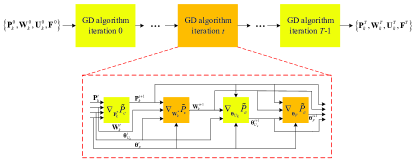
where {ฮผP,ฮผW,ฮผฮธU,ฮผฮธF}subscript๐œ‡๐‘ƒsubscript๐œ‡๐‘Šsubscript๐œ‡subscript๐œƒ๐‘ˆsubscript๐œ‡subscript๐œƒ๐น\{\mu_{P},\mu_{W},\mu_{\theta_{U}},\mu_{\theta_{F}}\} denote the step sizes employed in the GD iterations, and tโˆˆ{0,1,โ€ฆ}๐‘ก01โ€ฆt\in\{0,1,\ldots\} is the iteration index. The beamforming matrices are updated alternately until a certain convergence criterion is met. The iterative structure of the MSER-based GD algorithm structure is shown in Fig. 2.
Refer to caption
Figure 2: Structure of the proposed MSER-based iterative GD algorithm.

To guarantee the transmit power constraint (14b), at the end of each GD iteration, the overall digital transmit beamforming matrix ๐•๐•\mathbf{V} needs to be scaled as follows:

๐•โ†PTโ€–๐…๐•โ€–โ€‹๐•.โ†๐•subscript๐‘ƒ๐‘‡norm๐…๐•๐•\mathbf{V}\leftarrow\frac{\sqrt{P_{T}}}{\|\mathbf{F}\mathbf{V}\|}\,\mathbf{V}. (26)

The details of the proposed MSER-based GD hybrid beamforming design algorithm are summarized in Algorithm 1. The latter is devised to start its operation in the training mode, where a known training transmit symbol sequence is employed, and then switch to the decision-directed mode, wherein the estimated symbols are used for computation.

Algorithm 1 Gradient-descent algorithm for joint hybrid beamforming design
1: Set the tolerance of accuracy ฯตitalic-ฯต\epsilon, the maximum number of iterations T๐‘‡T, the size of the random sample J๐ฝJ, and the step sizes {ฮผP,ฮผW,ฮผฮธU,ฮผฮธF}subscript๐œ‡๐‘ƒsubscript๐œ‡๐‘Šsubscript๐œ‡subscript๐œƒ๐‘ˆsubscript๐œ‡subscript๐œƒ๐น\{\mu_{P},\mu_{W},\mu_{\theta_{U}},\mu_{\theta_{F}}\}. Set the iteration index to t=0๐‘ก0t=0.
2: Initialize ๐ksubscript๐๐‘˜\mathbf{P}_{k} to satisfy the power constraint. Initialize {๐–k,๐œฝUk,๐œฝF}subscript๐–๐‘˜subscript๐œฝsubscript๐‘ˆ๐‘˜subscript๐œฝ๐น\{\mathbf{W}_{k},\bm{\theta}_{U_{k}},\bm{\theta}_{F}\}.
3:repeat
4:ย ย ย ย  Update ๐kt+1superscriptsubscript๐๐‘˜๐‘ก1\mathbf{P}_{k}^{t+1} with fixed {๐–kt,๐œฝUkt,๐œฝFt}superscriptsubscript๐–๐‘˜๐‘กsuperscriptsubscript๐œฝsubscript๐‘ˆ๐‘˜๐‘กsuperscriptsubscript๐œฝ๐น๐‘ก\{\mathbf{W}_{k}^{t},\bm{\theta}_{U_{k}}^{t},\bm{\theta}_{F}^{t}\}, โˆ€kโˆˆ๐’ฆfor-all๐‘˜๐’ฆ\forall k\in\mathcal{K}, according to (22).
5:ย ย ย ย  Update ๐–kt+1superscriptsubscript๐–๐‘˜๐‘ก1\mathbf{W}_{k}^{t+1} with fixed {๐kt+1,๐œฝUkt,๐œฝFt}superscriptsubscript๐๐‘˜๐‘ก1superscriptsubscript๐œฝsubscript๐‘ˆ๐‘˜๐‘กsuperscriptsubscript๐œฝ๐น๐‘ก\{\mathbf{P}_{k}^{t+1},\bm{\theta}_{U_{k}}^{t},\bm{\theta}_{F}^{t}\}, โˆ€kโˆˆ๐’ฆfor-all๐‘˜๐’ฆ\forall k\in\mathcal{K}, according to (23).
6:ย ย ย ย  Update ๐œฝUkt+1superscriptsubscript๐œฝsubscript๐‘ˆ๐‘˜๐‘ก1\bm{\theta}_{U_{k}}^{t+1} with fixed {๐kt+1,๐–kt+1,๐œฝFt}superscriptsubscript๐๐‘˜๐‘ก1superscriptsubscript๐–๐‘˜๐‘ก1superscriptsubscript๐œฝ๐น๐‘ก\{\mathbf{P}_{k}^{t+1},\mathbf{W}_{k}^{t+1},\bm{\theta}_{F}^{t}\}, โˆ€kโˆˆ๐’ฆfor-all๐‘˜๐’ฆ\forall k\in\mathcal{K}, according to (24).
7:ย ย ย ย  Update ๐œฝFt+1superscriptsubscript๐œฝ๐น๐‘ก1\bm{\theta}_{F}^{t+1} with fixed {๐kt+1,๐–kt+1,๐œฝUkt+1}superscriptsubscript๐๐‘˜๐‘ก1superscriptsubscript๐–๐‘˜๐‘ก1superscriptsubscript๐œฝsubscript๐‘ˆ๐‘˜๐‘ก1\{\mathbf{P}_{k}^{t+1},\mathbf{W}_{k}^{t+1},\bm{\theta}_{U_{k}}^{t+1}\}, according to (25).
8:ย ย ย ย  Scale ๐kt+1superscriptsubscript๐๐‘˜๐‘ก1\mathbf{P}_{k}^{t+1} based on (26) to meet the transmit power constraint.
9:ย ย ย ย Update the iteration index: t=t+1๐‘ก๐‘ก1t=t+1.
10:untilย The objective function meets chosen convergence criterion or t>T๐‘ก๐‘‡t>{T}.

IV Proposed Deep-Unfolding NN for Hybrid AD Transceiver Design

The conventional MSER-based GD algorithms usually provide very slow convergence speed and therefore require a large number of iterations. Moreover, they suffer from performance degradation in the presence of channel state information (CSI) errors. To address these issues, we propose a deep-unfolding NN to jointly design the hybrid AD transceiver, where a small number of NN layers with trainable parameters can be employed while maintaining satisfactory performance. The proposed NN structure is inspired by the MSER-based GD algorithm, where the iterative algorithm is unfolded into a multi-layer structure and a number of adjustable step size and bias parameters are introduced in the FP. In the training stage, the relationship between the gradients of adjacent layers is derived according to the GCR in the BP. We then calculate the gradients w.r.t. the trainable parameters layer by layer and update these parameters based on the stochastic gradient descent (SGD) algorithm. In the testing stage, we perform the FP process based on the trained parameters for computing the AD beamforming matrices. The details of the FP and BP in the proposed NN are presented as follows.

IV-A Forward Propagation

In this subsection, we describe the structure of the proposed deep-unfolding NN which is induced by the MSER-based GD algorithm developed in Section III. In the iteration of the latter algorithm, the step sizes used for updating the hybrid AD beamforming matrices, i.e., {ฮผP,ฮผW,ฮผฮธU,ฮผฮธF}subscript๐œ‡๐‘ƒsubscript๐œ‡๐‘Šsubscript๐œ‡subscript๐œƒ๐‘ˆsubscript๐œ‡subscript๐œƒ๐น\{\mu_{P},\mu_{W},\mu_{\theta_{U}},\mu_{\theta_{F}}\} greatly affect the SER performance; furthermore, are usually determined based on experience and experiments. Therefore, in layer lโˆˆ{0,โ€ฆ,Lโˆ’1}๐‘™0โ€ฆ๐ฟ1l\in\{0,\ldots,L-1\} of the proposed NN, where L๐ฟL denotes the number of layers, we introduce the trainable matrix parameters {๐œถPkl,๐œถWkl,๐œถฮธUkl,๐œถฮธFl}superscriptsubscript๐œถsubscript๐‘ƒ๐‘˜๐‘™superscriptsubscript๐œถsubscript๐‘Š๐‘˜๐‘™superscriptsubscript๐œถsubscript๐œƒsubscript๐‘ˆ๐‘˜๐‘™superscriptsubscript๐œถsubscript๐œƒ๐น๐‘™\{\bm{\alpha}_{P_{k}}^{l},\bm{\alpha}_{W_{k}}^{l},\bm{\alpha}_{\theta_{U_{k}}}^{l},\bm{\alpha}_{\theta_{F}}^{l}\} as the learning rates to replace the step sizes of the MSER-based GD algorithm. Recall that the term ๐ฐi,kHโ€‹๐”kโ€‹๐‡kโ€‹๐…๐•๐•Hโ€‹๐…Hโ€‹๐‡kHโ€‹๐”kHโ€‹๐ฐi,kโ€‹ฯƒnsubscriptsuperscript๐ฐ๐ป๐‘–๐‘˜subscript๐”๐‘˜subscript๐‡๐‘˜superscript๐…๐•๐•๐ปsuperscript๐…๐ปsuperscriptsubscript๐‡๐‘˜๐ปsuperscriptsubscript๐”๐‘˜๐ปsubscript๐ฐ๐‘–๐‘˜subscript๐œŽ๐‘›\sqrt{\mathbf{w}^{H}_{i,k}\mathbf{U}_{k}\mathbf{H}_{k}\mathbf{F}\mathbf{V}\mathbf{V}^{H}\mathbf{F}^{H}\mathbf{H}_{k}^{H}\mathbf{U}_{k}^{H}\mathbf{w}_{i,k}}\sigma_{n} in (9) is set as a constant kernel width ฯฑitalic-ฯฑ\varrho in the MSER-based GD algorithm, which may cause performance loss. Hence, we replace ฯฑitalic-ฯฑ\varrho in (16)โ€“(19) by the set of trainable parameters {ฯPkl,ฯWkl,ฯUkl,ฯFl}superscriptsubscript๐œŒsubscript๐‘ƒ๐‘˜๐‘™superscriptsubscript๐œŒsubscript๐‘Š๐‘˜๐‘™superscriptsubscript๐œŒsubscript๐‘ˆ๐‘˜๐‘™superscriptsubscript๐œŒ๐น๐‘™\{\rho_{P_{k}}^{l},\rho_{W_{k}}^{l},\rho_{U_{k}}^{l},\rho_{F}^{l}\}. Moreover, to increase the degrees of freedom for the parameters, we introduce the trainable offset matrix parameters {๐ŽPkl,๐ŽWkl,๐ŽฮธUkl,๐ŽฮธFl}superscriptsubscript๐Žsubscript๐‘ƒ๐‘˜๐‘™superscriptsubscript๐Žsubscript๐‘Š๐‘˜๐‘™superscriptsubscript๐Žsubscript๐œƒsubscript๐‘ˆ๐‘˜๐‘™superscriptsubscript๐Žsubscript๐œƒ๐น๐‘™\{\mathbf{O}_{P_{k}}^{l},\mathbf{O}_{W_{k}}^{l},\mathbf{O}_{\theta_{U_{k}}}^{l},\mathbf{O}_{\theta_{F}}^{l}\} for the computation of the beamforming matrices. The update expressions for the proposed deep-unfolding NN are given by

๐kl+1=๐klโˆ’๐œถPklโˆ˜โˆ‡๐kโˆ—๐’ซ~el+๐ŽPkl,superscriptsubscript๐๐‘˜๐‘™1superscriptsubscript๐๐‘˜๐‘™superscriptsubscript๐œถsubscript๐‘ƒ๐‘˜๐‘™subscriptโˆ‡superscriptsubscript๐๐‘˜superscriptsubscript~๐’ซ๐‘’๐‘™superscriptsubscript๐Žsubscript๐‘ƒ๐‘˜๐‘™\mathbf{P}_{k}^{l+1}=\mathbf{P}_{k}^{l}-\bm{\alpha}_{P_{k}}^{l}\circ\nabla_{\mathbf{P}_{k}^{*}}\tilde{\mathcal{P}}_{e}^{l}+\mathbf{O}_{P_{k}}^{l},\vspace{-1mm} (27)
๐–kl+1=๐–klโˆ’๐œถWklโˆ˜โˆ‡๐–kโˆ—๐’ซ~el+๐ŽWkl,superscriptsubscript๐–๐‘˜๐‘™1superscriptsubscript๐–๐‘˜๐‘™superscriptsubscript๐œถsubscript๐‘Š๐‘˜๐‘™subscriptโˆ‡superscriptsubscript๐–๐‘˜superscriptsubscript~๐’ซ๐‘’๐‘™superscriptsubscript๐Žsubscript๐‘Š๐‘˜๐‘™\quad\ \mathbf{W}_{k}^{l+1}=\mathbf{W}_{k}^{l}-\bm{\alpha}_{W_{k}}^{l}\circ\nabla_{\mathbf{W}_{k}^{*}}\tilde{\mathcal{P}}_{e}^{l}+\mathbf{O}_{W_{k}}^{l},\vspace{-1mm} (28)
๐œฝUkl+1=๐œฝUklโˆ’๐œถฮธUklโˆ˜โˆ‡๐œฝUk๐’ซ~el+๐ŽฮธUkl,superscriptsubscript๐œฝsubscript๐‘ˆ๐‘˜๐‘™1superscriptsubscript๐œฝsubscript๐‘ˆ๐‘˜๐‘™superscriptsubscript๐œถsubscript๐œƒsubscript๐‘ˆ๐‘˜๐‘™subscriptโˆ‡subscript๐œฝsubscript๐‘ˆ๐‘˜superscriptsubscript~๐’ซ๐‘’๐‘™superscriptsubscript๐Žsubscript๐œƒsubscript๐‘ˆ๐‘˜๐‘™\quad\ \bm{\theta}_{U_{k}}^{l+1}=\bm{\theta}_{U_{k}}^{l}-\bm{\alpha}_{\theta_{U_{k}}}^{l}\circ\nabla_{\bm{\theta}_{U_{k}}}\tilde{\mathcal{P}}_{e}^{l}+\mathbf{O}_{\theta_{U_{k}}}^{l},\vspace{-1mm} (29)
๐œฝFl+1=๐œฝFlโˆ’๐œถฮธFlโˆ˜โˆ‡๐œฝF๐’ซ~el+๐ŽฮธFl,superscriptsubscript๐œฝ๐น๐‘™1superscriptsubscript๐œฝ๐น๐‘™superscriptsubscript๐œถsubscript๐œƒ๐น๐‘™subscriptโˆ‡subscript๐œฝ๐นsuperscriptsubscript~๐’ซ๐‘’๐‘™superscriptsubscript๐Žsubscript๐œƒ๐น๐‘™\bm{\theta}_{F}^{l+1}=\bm{\theta}_{F}^{l}-\bm{\alpha}_{\theta_{F}}^{l}\circ\nabla_{\bm{\theta}_{F}}\tilde{\mathcal{P}}_{e}^{l}+\mathbf{O}_{\theta_{F}}^{l},\vspace{-0mm} (30)

where {๐œถPkl,๐ŽPkl}โˆˆโ„‚Rtร—Dksuperscriptsubscript๐œถsubscript๐‘ƒ๐‘˜๐‘™superscriptsubscript๐Žsubscript๐‘ƒ๐‘˜๐‘™superscriptโ„‚subscript๐‘…๐‘กsubscript๐ท๐‘˜\{\bm{\alpha}_{P_{k}}^{l},\mathbf{O}_{P_{k}}^{l}\}\in\mathbb{C}^{R_{t}\times D_{k}}, {๐œถWkl,๐ŽWkl}โˆˆโ„‚Rr,kร—Dksuperscriptsubscript๐œถsubscript๐‘Š๐‘˜๐‘™superscriptsubscript๐Žsubscript๐‘Š๐‘˜๐‘™superscriptโ„‚subscript๐‘…๐‘Ÿ๐‘˜subscript๐ท๐‘˜\{\bm{\alpha}_{W_{k}}^{l},\mathbf{O}_{W_{k}}^{l}\}\in\mathbb{C}^{R_{r,k}\times D_{k}}, {๐œถฮธUkl,๐ŽฮธUkl}โˆˆโ„‚Rr,kร—Nr,ksuperscriptsubscript๐œถsubscript๐œƒsubscript๐‘ˆ๐‘˜๐‘™superscriptsubscript๐Žsubscript๐œƒsubscript๐‘ˆ๐‘˜๐‘™superscriptโ„‚subscript๐‘…๐‘Ÿ๐‘˜subscript๐‘๐‘Ÿ๐‘˜\{\bm{\alpha}_{\theta_{U_{k}}}^{l},\mathbf{O}_{\theta_{U_{k}}}^{l}\}\in\mathbb{C}^{R_{r,k}\times N_{r,k}}, {๐œถฮธFl,๐ŽฮธFl}โˆˆโ„‚Ntร—Rtsuperscriptsubscript๐œถsubscript๐œƒ๐น๐‘™superscriptsubscript๐Žsubscript๐œƒ๐น๐‘™superscriptโ„‚subscript๐‘๐‘กsubscript๐‘…๐‘ก\{\bm{\alpha}_{\theta_{F}}^{l},\mathbf{O}_{\theta_{F}}^{l}\}\in\mathbb{C}^{N_{t}\times R_{t}}, and {โˆ‡๐kโˆ—๐’ซ~el,โˆ‡๐–kโˆ—๐’ซ~el,โˆ‡๐œฝUk๐’ซ~el,โˆ‡๐œฝF๐’ซ~el}subscriptโˆ‡superscriptsubscript๐๐‘˜superscriptsubscript~๐’ซ๐‘’๐‘™subscriptโˆ‡superscriptsubscript๐–๐‘˜superscriptsubscript~๐’ซ๐‘’๐‘™subscriptโˆ‡subscript๐œฝsubscript๐‘ˆ๐‘˜superscriptsubscript~๐’ซ๐‘’๐‘™subscriptโˆ‡subscript๐œฝ๐นsuperscriptsubscript~๐’ซ๐‘’๐‘™\{\nabla_{\mathbf{P}_{k}^{*}}\tilde{\mathcal{P}}_{e}^{l},\nabla_{\mathbf{W}_{k}^{*}}\tilde{\mathcal{P}}_{e}^{l},\nabla_{\bm{\theta}_{U_{k}}}\tilde{\mathcal{P}}_{e}^{l},\nabla_{\bm{\theta}_{F}}\tilde{\mathcal{P}}_{e}^{l}\} denote the gradients w.r.t. the beamforming matrices in the l๐‘™l-th layer.

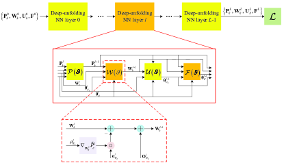
The structure of the proposed deep-unfolding NN induced by the MSER-based GD algorithm is illustrated in Fig. 3. Compared with Fig. 2, we can see that this structure is developed by unfolding the iterative GD algorithm into a multi-layer, comprised of L๐ฟL successive layers (top). The enlarged part in the red solid rectangle (middle) presents the common details of each layer in the deep-unfolding NN, where the operations ๐’ซโ€‹(ฯ‘)๐’ซitalic-ฯ‘\mathcal{P}(\vartheta), ๐’ฒโ€‹(ฯ‘)๐’ฒitalic-ฯ‘\mathcal{W}(\vartheta), ๐’ฐโ€‹(ฯ‘)๐’ฐitalic-ฯ‘\mathcal{U}(\vartheta), and โ„ฑโ€‹(ฯ‘)โ„ฑitalic-ฯ‘\mathcal{F}(\vartheta) represent (27)โ€“(30), respectively. Specifically, in layer lโˆˆ{0,โ€ฆ,Lโˆ’1}๐‘™0โ€ฆ๐ฟ1l\in\{0,\ldots,L-1\}, we first update the digital beamforming matrices ๐ksubscript๐๐‘˜\mathbf{P}_{k} and ๐–ksubscript๐–๐‘˜\mathbf{W}_{k} successively, followed by the analog beamforming phase matrices ๐œฝUksubscript๐œฝsubscript๐‘ˆ๐‘˜\bm{\theta}_{U_{k}} and ๐œฝFsubscript๐œฝ๐น\bm{\theta}_{F}. For each one of these updates, the enlarged diagram in the red dotted rectanlge (bottom) illustrates how the GD updates make use of the additional parameters ๐œถXlsuperscriptsubscript๐œถ๐‘‹๐‘™\bm{\alpha}_{X}^{l}, ฯXlsuperscriptsubscript๐œŒ๐‘‹๐‘™\rho_{X}^{l}, and ๐ŽXlsuperscriptsubscript๐Ž๐‘‹๐‘™\mathbf{O}_{X}^{l}, where symbol Xโˆˆ{Pk,Wk,ฮธUk,ฮธF}๐‘‹subscript๐‘ƒ๐‘˜subscript๐‘Š๐‘˜subscript๐œƒsubscript๐‘ˆ๐‘˜subscript๐œƒ๐นX\in\{P_{k},W_{k},\theta_{U_{k}},\theta_{F}\}. The beamforming matrices in the last layer are served as the NN outputs and are conveyed to the loss function. Since ๐œฝFsubscript๐œฝ๐น\bm{\theta}_{F} is the last updated parameter matrix, the iteration rule of ๐œฝFLsuperscriptsubscript๐œฝ๐น๐ฟ\bm{\theta}_{F}^{L} adopts the original formula (25) without introducing additional parameters.
Refer to caption
Figure 3: Structure of the proposed deep-unfolding NN induced by the MSER-based GD algorithm.

Since the channel matrices ๐‡ksubscript๐‡๐‘˜\mathbf{H}_{k} are random by nature, the final loss function incorporates an expectation operation ๐”ผ๐‡subscript๐”ผ๐‡\mathbb{E}_{\mathbf{H}} over the ensemble of channel matrices. Hence, the loss function โ„’โ„’\mathcal{L} in the top-right corner of Fig. 3 is modified as

โ„’=โˆ‘k=1K๐”ผ๐‡{1Jโ€‹ฯ€โˆ‘i=1Dkโˆ‘j=1J(โˆซโˆ’โˆžโˆ’โ„œโก{bยฏi,kqj}โ€‹โ„œโก{bi,k}2โ€‹ฯeโˆ’s2ds+โˆซโˆ’โˆžโˆ’โ„‘โก{bยฏi,kqj}โ€‹โ„‘โก{bi,k}2โ€‹ฯeโˆ’s2ds)}.โ„’superscriptsubscript๐‘˜1๐พsubscript๐”ผ๐‡1๐ฝ๐œ‹superscriptsubscript๐‘–1subscript๐ท๐‘˜superscriptsubscript๐‘—1๐ฝsuperscriptsubscriptsubscriptsuperscriptยฏ๐‘subscript๐‘ž๐‘—๐‘–๐‘˜subscript๐‘๐‘–๐‘˜2๐œŒsuperscript๐‘’superscript๐‘ 2๐‘‘๐‘ superscriptsubscriptsubscriptsuperscriptยฏ๐‘subscript๐‘ž๐‘—๐‘–๐‘˜subscript๐‘๐‘–๐‘˜2๐œŒsuperscript๐‘’superscript๐‘ 2๐‘‘๐‘ \begin{split}\mathcal{L}=\sum\limits_{k=1}^{K}\mathbb{E}_{\mathbf{H}}&\Bigg{\{}\frac{1}{J\sqrt{\pi}}\sum\limits_{i=1}^{D_{k}}\sum\limits_{{j}=1}^{J}\Big{(}\int_{-\infty}^{-\frac{\Re\{\bar{b}^{q_{j}}_{i,k}\}\Re\{b_{i,k}\}}{\sqrt{2}\rho}}e^{-s^{2}}\!\ ds\\ &+\int_{-\infty}^{-\frac{\Im\{\bar{b}^{q_{j}}_{i,k}\}\Im\{b_{i,k}\}}{\sqrt{2}\rho}}e^{-s^{2}}\!\ ds\Big{)}\Bigg{\}}.\end{split} (31)

As mentioned in Section III, ๐•=[๐1,โ€ฆ,๐K]๐•subscript๐1โ€ฆsubscript๐๐พ\mathbf{V}=[\mathbf{P}_{1},\ldots,\mathbf{P}_{K}] is scaled based on (26) in each layer to satisfy the transmit power constraint, which also helps avoid gradient explosion.

IV-B Back Propagation

Since the conventional platforms for implementation and training of NN (e.g. Pytorch or Tensorflow) are not designed to handle loss functions in the form of integrals, we seek to propose a novel method to compute the gradients in closed-form, which is more accurate and efficient. In the BP, we derive the recursive relation between the gradients of adjacent layers based on the GCR which is given in Appendix A, and then compute the gradients w.r.t. the trainable parameters.

Let {๐†Pkl,๐†Wkl,๐†Ukl,๐†Ukโˆ—l,๐†Fl,๐†Fโˆ—l}superscriptsubscript๐†subscript๐‘ƒ๐‘˜๐‘™superscriptsubscript๐†subscript๐‘Š๐‘˜๐‘™superscriptsubscript๐†subscript๐‘ˆ๐‘˜๐‘™superscriptsubscript๐†subscriptsuperscript๐‘ˆ๐‘˜๐‘™superscriptsubscript๐†๐น๐‘™superscriptsubscript๐†superscript๐น๐‘™\{\mathbf{G}_{P_{k}}^{l},\mathbf{G}_{W_{k}}^{l},\mathbf{G}_{U_{k}}^{l},\mathbf{G}_{U^{*}_{k}}^{l},\mathbf{G}_{F}^{l},\mathbf{G}_{F^{*}}^{l}\} denote the gradients w.r.t. the hybrid AD beamforming matrices in the l๐‘™l-th layer. By taking the derivative of (31), we can calculate the gradients w.r.t. ๐…Lsuperscript๐…๐ฟ\mathbf{F}^{L} and (๐…โˆ—)Lsuperscriptsuperscript๐…๐ฟ(\mathbf{F}^{*})^{L} in the last layer as

๐†FL=(โˆ‡๐…๐’ซ~eL)H,๐†Fโˆ—L=(โˆ‡๐…โˆ—๐’ซ~eL)H.formulae-sequencesuperscriptsubscript๐†๐น๐ฟsuperscriptsubscriptโˆ‡๐…superscriptsubscript~๐’ซ๐‘’๐ฟ๐ปsuperscriptsubscript๐†superscript๐น๐ฟsuperscriptsubscriptโˆ‡superscript๐…superscriptsubscript~๐’ซ๐‘’๐ฟ๐ป\mathbf{G}_{F}^{L}=(\nabla_{\mathbf{F}}\tilde{\mathcal{P}}_{e}^{L})^{H},\quad\mathbf{G}_{F^{*}}^{L}=(\nabla_{\mathbf{F}^{*}}\tilde{\mathcal{P}}_{e}^{L})^{H}.\vspace{-2mm} (32)

By differentiating on both sides of (20) and (21), it is readily seen that ๐†ฮธUklsuperscriptsubscript๐†subscript๐œƒsubscript๐‘ˆ๐‘˜๐‘™\mathbf{G}_{\theta_{U_{k}}}^{l} and ๐†ฮธFlsuperscriptsubscript๐†subscript๐œƒ๐น๐‘™\mathbf{G}_{\theta_{F}}^{l} can be computed based on {๐†Ukl,๐†Ukโˆ—l}superscriptsubscript๐†subscript๐‘ˆ๐‘˜๐‘™superscriptsubscript๐†superscriptsubscript๐‘ˆ๐‘˜๐‘™\{\mathbf{G}_{U_{k}}^{l},\mathbf{G}_{{U_{k}^{*}}}^{l}\} and {๐†Fl,๐†Fโˆ—l}superscriptsubscript๐†๐น๐‘™superscriptsubscript๐†superscript๐น๐‘™\{\mathbf{G}_{F}^{l},\mathbf{G}_{F^{*}}^{l}\}, respectively, as

๐†ฮธUkl=๐†Uklโˆ˜jโ€‹๐”kTโˆ’๐†Ukโˆ—lโˆ˜jโ€‹๐”kโˆ—,superscriptsubscript๐†subscript๐œƒsubscript๐‘ˆ๐‘˜๐‘™superscriptsubscript๐†subscript๐‘ˆ๐‘˜๐‘™๐‘—superscriptsubscript๐”๐‘˜๐‘‡superscriptsubscript๐†superscriptsubscript๐‘ˆ๐‘˜๐‘™๐‘—superscriptsubscript๐”๐‘˜\quad\mathbf{G}_{\theta_{U_{k}}}^{l}=\mathbf{G}_{U_{k}}^{l}\circ j\mathbf{U}_{k}^{T}-\mathbf{G}_{U_{k}^{*}}^{l}\circ j\mathbf{U}_{k}^{*},\vspace{-0mm} (33)
๐†ฮธFl=๐†Flโˆ˜jโ€‹๐…Tโˆ’๐†Fโˆ—lโˆ˜jโ€‹๐…โˆ—.superscriptsubscript๐†subscript๐œƒ๐น๐‘™superscriptsubscript๐†๐น๐‘™๐‘—superscript๐…๐‘‡superscriptsubscript๐†superscript๐น๐‘™๐‘—superscript๐…\mathbf{G}_{\theta_{F}}^{l}=\mathbf{G}_{F}^{l}\circ j\mathbf{F}^{T}-\mathbf{G}_{F^{*}}^{l}\circ j\mathbf{F}^{*}.\vspace{-0mm} (34)

Next, we derive the recursive relationship between the gradients w.r.t. the hybrid beamforming matrices in the (l+1๐‘™1l+1)-th layer and the l๐‘™l-th layer. To this end, we first take the derivative on both sides of the equations (27)โ€“(30) and apply the differential multiplication rules. Let us first expand (27) and provide the relationship between ๐†Pkl+1superscriptsubscript๐†subscript๐‘ƒ๐‘˜๐‘™1\mathbf{G}_{P_{k}}^{l+1} and ๐†Pklsuperscriptsubscript๐†subscript๐‘ƒ๐‘˜๐‘™\mathbf{G}_{P_{k}}^{l}; the corresponding relations for the other matrices can be derived similarly. To simplify the presentation, we omit the index of data stream i๐‘–i, the index of transmit vector qjsubscript๐‘ž๐‘—q_{j}, and the index of iteration t๐‘กt. Based on (27) and the GCR shown in Appendix A, we have

Tr{๐†Pkl+1d๐kl+1}=1Jโˆ‘j=1JTr{๐†Pkl+1d๐klโˆ’bkHB๐†Pkl+1โˆ˜(๐œถPkl)T(๐…l)H๐‡kH(๐”kl)H๐–klโˆ˜[bk(๐–kl)H๐”kl๐‡k๐…ldโ€‹๐kl+๐ƒHโ€‹(๐”kl)Hโ€‹dโ€‹๐–kl+๐‚โ€‹(๐–kl)Hโ€‹๐”klโ€‹๐‡kโ€‹dโ€‹๐…l+๐ƒ(๐–kl)Hโ€‹dโ€‹๐”kl+๐‡kHโ€‹(๐”kl)Hโ€‹๐–klโ€‹๐‚Hโ€‹dโ€‹(๐…H)l+๐–klโ€‹๐ƒHd(๐”kH)l]+bkHA๐†Pkl+1โˆ˜(๐œถPkl)T(๐…l)H๐‡kH(๐”kl)Hdโ€‹๐–kl+bkHโ€‹Aโ€‹๐‡kHโ€‹(๐”kl)Hโ€‹๐–klโ€‹๐†Pkl+1โˆ˜(๐œถPkl)Tโ€‹dโ€‹(๐…H)l+bkHA๐–kl๐†Pkl+1โˆ˜(๐œถPkl)T(๐…l)H๐‡kHd(๐”kH)l},Trsuperscriptsubscript๐†subscript๐‘ƒ๐‘˜๐‘™1๐‘‘superscriptsubscript๐๐‘˜๐‘™11๐ฝsuperscriptsubscript๐‘—1๐ฝTrsuperscriptsubscript๐†subscript๐‘ƒ๐‘˜๐‘™1๐‘‘superscriptsubscript๐๐‘˜๐‘™superscriptsubscript๐‘๐‘˜๐ป๐ตsuperscriptsubscript๐†subscript๐‘ƒ๐‘˜๐‘™1superscriptsuperscriptsubscript๐œถsubscript๐‘ƒ๐‘˜๐‘™๐‘‡superscriptsuperscript๐…๐‘™๐ปsuperscriptsubscript๐‡๐‘˜๐ปsuperscriptsuperscriptsubscript๐”๐‘˜๐‘™๐ปsubscriptsuperscript๐–๐‘™๐‘˜delimited-[]subscript๐‘๐‘˜superscriptsuperscriptsubscript๐–๐‘˜๐‘™๐ปsuperscriptsubscript๐”๐‘˜๐‘™subscript๐‡๐‘˜superscript๐…๐‘™๐‘‘superscriptsubscript๐๐‘˜๐‘™superscript๐ƒ๐ปsuperscriptsuperscriptsubscript๐”๐‘˜๐‘™๐ป๐‘‘superscriptsubscript๐–๐‘˜๐‘™๐‚superscriptsuperscriptsubscript๐–๐‘˜๐‘™๐ปsuperscriptsubscript๐”๐‘˜๐‘™subscript๐‡๐‘˜๐‘‘superscript๐…๐‘™๐ƒsuperscriptsuperscriptsubscript๐–๐‘˜๐‘™๐ป๐‘‘superscriptsubscript๐”๐‘˜๐‘™superscriptsubscript๐‡๐‘˜๐ปsuperscriptsuperscriptsubscript๐”๐‘˜๐‘™๐ปsuperscriptsubscript๐–๐‘˜๐‘™superscript๐‚๐ป๐‘‘superscriptsuperscript๐…๐ป๐‘™superscriptsubscript๐–๐‘˜๐‘™superscript๐ƒ๐ป๐‘‘superscriptsuperscriptsubscript๐”๐‘˜๐ป๐‘™superscriptsubscript๐‘๐‘˜๐ป๐ดsuperscriptsubscript๐†subscript๐‘ƒ๐‘˜๐‘™1superscriptsuperscriptsubscript๐œถsubscript๐‘ƒ๐‘˜๐‘™๐‘‡superscriptsuperscript๐…๐‘™๐ปsuperscriptsubscript๐‡๐‘˜๐ปsuperscriptsuperscriptsubscript๐”๐‘˜๐‘™๐ป๐‘‘superscriptsubscript๐–๐‘˜๐‘™superscriptsubscript๐‘๐‘˜๐ป๐ดsuperscriptsubscript๐‡๐‘˜๐ปsuperscriptsuperscriptsubscript๐”๐‘˜๐‘™๐ปsuperscriptsubscript๐–๐‘˜๐‘™superscriptsubscript๐†subscript๐‘ƒ๐‘˜๐‘™1superscriptsuperscriptsubscript๐œถsubscript๐‘ƒ๐‘˜๐‘™๐‘‡๐‘‘superscriptsuperscript๐…๐ป๐‘™superscriptsubscript๐‘๐‘˜๐ป๐ดsuperscriptsubscript๐–๐‘˜๐‘™superscriptsubscript๐†subscript๐‘ƒ๐‘˜๐‘™1superscriptsuperscriptsubscript๐œถsubscript๐‘ƒ๐‘˜๐‘™๐‘‡superscriptsuperscript๐…๐‘™๐ปsuperscriptsubscript๐‡๐‘˜๐ป๐‘‘superscriptsuperscriptsubscript๐”๐‘˜๐ป๐‘™\begin{split}&\!\!\!\!\!{\rm Tr}\left\{\mathbf{G}_{P_{k}}^{l+1}d\mathbf{P}_{k}^{l+1}\right\}=\frac{1}{J}\sum\limits_{j=1}^{J}{\rm Tr}\left\{\mathbf{G}_{P_{k}}^{l+1}d\mathbf{P}_{k}^{l}-b_{k}^{H}B\,\mathbf{G}_{P_{k}}^{l+1}\circ\right.\\ &\!\!\!\!\!(\bm{\alpha}_{P_{k}}^{l})^{T}\,\left.(\mathbf{F}^{l})^{H}\mathbf{H}_{k}^{H}(\mathbf{U}_{k}^{l})^{H}\mathbf{W}^{l}_{k}\circ\left[b_{k}\,(\mathbf{W}_{k}^{l})^{H}\mathbf{U}_{k}^{l}\mathbf{H}_{k}\mathbf{F}^{l}\right.\right.\\ &\!\!\!\!\!d\mathbf{P}_{k}^{l}+\mathbf{D}^{H}(\mathbf{U}_{k}^{l})^{H}d\mathbf{W}_{k}^{l}+\mathbf{C}(\mathbf{W}_{k}^{l})^{H}\mathbf{U}_{k}^{l}\mathbf{H}_{k}\,d\mathbf{F}^{l}+\mathbf{D}\\ &\!\!\!\!\!\left.\left.(\mathbf{W}_{k}^{l})^{H}d\mathbf{U}_{k}^{l}+\mathbf{H}_{k}^{H}(\mathbf{U}_{k}^{l})^{H}\mathbf{W}_{k}^{l}\mathbf{C}^{H}d(\mathbf{F}^{H})^{l}+\mathbf{W}_{k}^{l}\mathbf{D}^{H}\right.\right.\\ &\!\!\!\!\!\left.\left.d(\mathbf{U}_{k}^{H})^{l}\right]+b_{k}^{H}A\,\mathbf{G}_{P_{k}}^{l+1}\circ(\bm{\alpha}_{P_{k}}^{l})^{T}(\mathbf{F}^{l})^{H}\mathbf{H}_{k}^{H}(\mathbf{U}_{k}^{l})^{H}\right.\\ &\!\!\!\!\!\left.d\mathbf{W}_{k}^{l}+b_{k}^{H}A\,\mathbf{H}_{k}^{H}(\mathbf{U}_{k}^{l})^{H}\mathbf{W}_{k}^{l}\mathbf{G}_{P_{k}}^{l+1}\circ(\bm{\alpha}_{P_{k}}^{l})^{T}d(\mathbf{F}^{H})^{l}\right.\\ &\!\!\!\!\!\left.+b_{k}^{H}A\,\mathbf{W}_{k}^{l}\mathbf{G}_{P_{k}}^{l+1}\circ(\bm{\alpha}_{P_{k}}^{l})^{T}(\mathbf{F}^{l})^{H}\mathbf{H}_{k}^{H}d(\mathbf{U}_{k}^{H})^{l}\right\},\end{split}\vspace{-4mm} (35)

where Aโ‰œโ„œโก{bk}2โ€‹ฯ€โ€‹ฯPklโ€‹eโˆ’|โ„œโก{bยฏk}|22โ€‹(ฯPkl)2โ‰œ๐ดsubscript๐‘๐‘˜2๐œ‹superscriptsubscript๐œŒsubscript๐‘ƒ๐‘˜๐‘™superscript๐‘’superscriptsubscriptยฏ๐‘๐‘˜22superscriptsuperscriptsubscript๐œŒsubscript๐‘ƒ๐‘˜๐‘™2A\triangleq\frac{\Re\{b_{k}\}}{\sqrt{2\pi}\rho_{P_{k}}^{l}}\,e^{-\frac{|\Re\{\bar{b}_{k}\}|^{2}}{2(\rho_{P_{k}}^{l})^{2}}}, Bโ‰œAโ€‹โ„œโก{bk}(ฯPkl)2โ‰œ๐ต๐ดsubscript๐‘๐‘˜superscriptsuperscriptsubscript๐œŒsubscript๐‘ƒ๐‘˜๐‘™2B\triangleq A\,\dfrac{\Re\{b_{k}\}}{(\rho_{P_{k}}^{l})^{2}}, ๐‚โ‰œโˆ‘i=1Dk๐ฉi,klโ€‹bi,kโ‰œ๐‚superscriptsubscript๐‘–1subscript๐ท๐‘˜superscriptsubscript๐ฉ๐‘–๐‘˜๐‘™subscript๐‘๐‘–๐‘˜\mathbf{C}\triangleq\sum\limits_{i=1}^{D_{k}}\mathbf{p}_{i,k}^{l}b_{i,k}, and ๐ƒโ‰œ๐‡kโ€‹๐…lโ€‹๐‚โ‰œ๐ƒsubscript๐‡๐‘˜superscript๐…๐‘™๐‚\mathbf{D}\triangleq\mathbf{H}_{k}\mathbf{F}^{l}\mathbf{C}. By proceeding in the same way with (28)โ€“(30), we obtain all the necessary relations linking the various gradients in adjacent layers.

By isolating and rearranging corresponding terms in dโ€‹๐kl๐‘‘superscriptsubscript๐๐‘˜๐‘™d\mathbf{P}_{k}^{l}, we obtain the desired relationship for ๐†Pklsuperscriptsubscript๐†subscript๐‘ƒ๐‘˜๐‘™\mathbf{G}_{P_{k}}^{l} as

๐†Pkl=โˆ’1Jโˆ‘j=1J(bkHB๐†Pkl+1โˆ˜(๐œถPkl)T(๐…l)H๐‡kH(๐”kl)H.โˆ˜๐–klโ€‹๐„โˆ’Bโ€‹๐†Wkl+1โˆ˜(๐œถWkl)Tโ€‹๐”klโ€‹๐ƒโˆ˜๐„+bkโ€‹Aโ€‹[๐†Fl+1โˆ˜(๐œถฮธFl)Tโ€‹๐‡kTโ€‹(๐”kl+1)Tโ€‹(๐–kl)H]Tโˆ’bkA๐†Wkl+1โˆ˜(๐œถWkl)T๐”kl๐‡k๐…l+bkA[(๐…l)T๐‡kT.๐†Ukl+1โˆ˜(๐œถฮธUkl)T(๐–kl)H]Tโˆ’B๐ƒT๐†Ukl+1โˆ˜(๐œถฮธUkl)T(๐–kl)Hโˆ˜๐„โˆ’Bโ€‹๐‚Hโ€‹๐†Fโˆ—l+1โˆ˜(๐œถฮธFl)Tโ€‹๐‡kHโ€‹(๐”kl+1)H๐–klโˆ˜๐„โˆ’Bโ€‹๐ƒHโ€‹๐†Ukโˆ—l+1โˆ˜(๐œถฮธUkl)Tโ€‹๐–klโˆ˜๐„โˆ’Bโ€‹๐‚T๐†Fl+1โˆ˜(๐œถฮธFl)T๐‡kT(๐”kl+1)T(๐–kl)Hโˆ˜๐„)+๐†Pkl+1,\begin{split}&\!\!\!\mathbf{G}_{P_{k}}^{l}=-\frac{1}{J}\sum\limits_{j=1}^{J}\Big{(}b_{k}^{H}B\,\mathbf{G}_{P_{k}}^{l+1}\circ(\bm{\alpha}_{P_{k}}^{l})^{T}(\mathbf{F}^{l})^{H}\mathbf{H}_{k}^{H}(\mathbf{U}_{k}^{l})^{H}\Big{.}\\ &\ \circ\mathbf{W}_{k}^{l}\mathbf{E}-B\,\mathbf{G}_{W_{k}}^{l+1}\circ(\bm{\alpha}_{W_{k}}^{l})^{T}\mathbf{U}^{l}_{k}\mathbf{D}\circ\mathbf{E}\\ &\ +b_{k}A\,\left[\mathbf{G}_{F}^{l+1}\circ(\bm{\alpha}_{\theta_{F}}^{l})^{T}\mathbf{H}_{k}^{T}(\mathbf{U}_{k}^{l+1})^{T}(\mathbf{W}_{k}^{l})^{H}\right]^{T}\\ &\ -b_{k}A\,\mathbf{G}_{W_{k}}^{l+1}\circ(\bm{\alpha}_{W_{k}}^{l})^{T}\mathbf{U}_{k}^{l}\mathbf{H}_{k}\mathbf{F}^{l}+b_{k}A\,[(\mathbf{F}^{l})^{T}\mathbf{H}_{k}^{T}\\ \Big{.}&\,\ \mathbf{G}_{U_{k}}^{l+1}\circ(\bm{\alpha}_{\theta_{U_{k}}}^{l})^{T}(\mathbf{W}_{k}^{l})^{H}]^{T}-B\,\mathbf{D}^{T}\mathbf{G}_{U_{k}}^{l+1}\circ(\bm{\alpha}_{\theta_{U_{k}}}^{l})^{T}\\ &\,\ (\mathbf{W}_{k}^{l})^{H}\circ\mathbf{E}-B\,\mathbf{C}^{H}\mathbf{G}_{F^{*}}^{l+1}\circ(\bm{\alpha}_{\theta_{F}}^{l})^{T}\mathbf{H}_{k}^{H}(\mathbf{U}_{k}^{l+1})^{H}\\ &\,\ \mathbf{W}_{k}^{l}\circ\mathbf{E}-B\,\mathbf{D}^{H}\mathbf{G}_{U_{k}^{*}}^{l+1}\circ(\bm{\alpha}_{\theta_{U_{k}}}^{l})^{T}\mathbf{W}_{k}^{l}\circ\mathbf{E}-B\,\mathbf{C}^{T}\\ &\ \ \mathbf{G}_{F}^{l+1}\circ(\bm{\alpha}_{\theta_{F}}^{l})^{T}\mathbf{H}_{k}^{T}(\mathbf{U}_{k}^{l+1})^{T}(\mathbf{W}_{k}^{l})^{H}\circ\mathbf{E}\Big{)}+\mathbf{G}_{P_{k}}^{l+1},\end{split} (36)

where ๐„โ‰œbkโ€‹(๐–kl)Hโ€‹๐”klโ€‹๐‡kโ€‹๐…lโ‰œ๐„subscript๐‘๐‘˜superscriptsuperscriptsubscript๐–๐‘˜๐‘™๐ปsuperscriptsubscript๐”๐‘˜๐‘™subscript๐‡๐‘˜superscript๐…๐‘™\mathbf{E}\triangleq b_{k}\,(\mathbf{W}_{k}^{l})^{H}\mathbf{U}_{k}^{l}\mathbf{H}_{k}\mathbf{F}^{l}. The gradients w.r.t. the other beamforming matrices in the l๐‘™l-th layer can be obtained similarly. Furthermore, the gradients w.r.t. the introduced parameters in each layer are computed based on (27)โ€“(30). The detailed expressions of {โˆ‡๐œถX๐’ซ~el,โˆ‡ฯX๐’ซ~el,โˆ‡๐ŽX๐’ซ~el}subscriptโˆ‡subscript๐œถ๐‘‹superscriptsubscript~๐’ซ๐‘’๐‘™subscriptโˆ‡subscript๐œŒ๐‘‹superscriptsubscript~๐’ซ๐‘’๐‘™subscriptโˆ‡subscript๐Ž๐‘‹superscriptsubscript~๐’ซ๐‘’๐‘™\{\nabla_{\bm{\alpha}_{X}}\tilde{\mathcal{P}}_{e}^{l},\nabla_{\rho_{X}}\tilde{\mathcal{P}}_{e}^{l},\nabla_{\mathbf{O}_{X}}\tilde{\mathcal{P}}_{e}^{l}\}, where Xโˆˆ{Pk,Wk,ฮธUk,ฮธF}๐‘‹subscript๐‘ƒ๐‘˜subscript๐‘Š๐‘˜subscript๐œƒsubscript๐‘ˆ๐‘˜subscript๐œƒ๐นX\in\{P_{k},W_{k},\theta_{U_{k}},\theta_{F}\}, are shown in Appendix B.

We calculate the average gradient in a batch and implement the SGD method to update the trainable parameters, such as in, e.g., ๐œถPkl,t+1=๐œถPkl,tโˆ’ฮผฮฑPktโ€‹โˆ‡๐œถPkt๐’ซ~elsuperscriptsubscript๐œถsubscript๐‘ƒ๐‘˜๐‘™๐‘ก1superscriptsubscript๐œถsubscript๐‘ƒ๐‘˜๐‘™๐‘กsuperscriptsubscript๐œ‡subscript๐›ผsubscript๐‘ƒ๐‘˜๐‘กsubscriptโˆ‡superscriptsubscript๐œถsubscript๐‘ƒ๐‘˜๐‘กsuperscriptsubscript~๐’ซ๐‘’๐‘™\bm{\alpha}_{P_{k}}^{l,t+1}=\bm{\alpha}_{P_{k}}^{l,t}-\mu_{\alpha_{P_{k}}}^{t}\nabla_{\bm{\alpha}_{P_{k}}^{t}}\tilde{\mathcal{P}}_{e}^{l}, where ฮผฮฑPktsuperscriptsubscript๐œ‡subscript๐›ผsubscript๐‘ƒ๐‘˜๐‘ก\mu_{\alpha_{P_{k}}}^{t} denotes the step size of the update in SGD of ๐œถPklsuperscriptsubscript๐œถsubscript๐‘ƒ๐‘˜๐‘™\bm{\alpha}_{P_{k}}^{l} in the t๐‘กt-th iteration, which incorporates an attenuation factor dependent on iteration t๐‘กt. In order to avoid vanishing gradient problem in the BP, normalization is employed after the update of {๐†Pkl,๐†Wkl,๐†Ukl,๐†Ukโˆ—l,๐†Fl,๐†Fโˆ—l}superscriptsubscript๐†subscript๐‘ƒ๐‘˜๐‘™superscriptsubscript๐†subscript๐‘Š๐‘˜๐‘™superscriptsubscript๐†subscript๐‘ˆ๐‘˜๐‘™superscriptsubscript๐†subscriptsuperscript๐‘ˆ๐‘˜๐‘™superscriptsubscript๐†๐น๐‘™superscriptsubscript๐†superscript๐น๐‘™\{\mathbf{G}_{P_{k}}^{l},\mathbf{G}_{W_{k}}^{l},\mathbf{G}_{U_{k}}^{l},\mathbf{G}_{U^{*}_{k}}^{l},\mathbf{G}_{F}^{l},\mathbf{G}_{F^{*}}^{l}\}. The specific rule of normalizing ๐†Pklsuperscriptsubscript๐†subscript๐‘ƒ๐‘˜๐‘™\mathbf{G}_{P_{k}}^{l} is given as

๐†Pklโ†Kโ€‹๐†Pklโˆ‘kโ€–๐†Pklโ€–.โ†superscriptsubscript๐†subscript๐‘ƒ๐‘˜๐‘™๐พsuperscriptsubscript๐†subscript๐‘ƒ๐‘˜๐‘™subscript๐‘˜normsuperscriptsubscript๐†subscript๐‘ƒ๐‘˜๐‘™\mathbf{G}_{P_{k}}^{l}\leftarrow\dfrac{K\mathbf{G}_{P_{k}}^{l}}{\sum\limits_{k}\!\left\|\mathbf{G}_{P_{k}}^{l}\right\|}.\vspace{-2mm} (37)

The gradients w.r.t. the other variables can be computed in the same way. The trainable parameters are initialized randomly and the beamforming matrices {๐k0,๐–k0,๐œฝUk0,๐œฝF0}superscriptsubscript๐๐‘˜0superscriptsubscript๐–๐‘˜0superscriptsubscript๐œฝsubscript๐‘ˆ๐‘˜0superscriptsubscript๐œฝ๐น0\{\mathbf{P}_{k}^{0},\mathbf{W}_{k}^{0},\bm{\theta}_{U_{k}}^{0},\bm{\theta}_{F}^{0}\} are initialized based on the conventional channel alignment method [6]. The training process of the deep-unfolding NN is shown in Algorithm 2, where โ„‹โ‰œ{๐‡k1,๐‡k2,โ€ฆ,๐‡kN}โ‰œโ„‹superscriptsubscript๐‡๐‘˜1superscriptsubscript๐‡๐‘˜2โ€ฆsuperscriptsubscript๐‡๐‘˜๐‘\mathcal{H}\triangleq\{\mathbf{H}_{k}^{1},\mathbf{H}_{k}^{2},\ldots,\mathbf{H}_{k}^{N}\} and N๐‘N is determined by simulations.

Algorithm 2 Training process of the proposed deep-unfolding NN induced by GD algorithm
1: Generate training data set {๐’ณ,โ„‹}๐’ณโ„‹\{\mathcal{X},\mathcal{H}\}. Set tolerance of accuracy ฯตitalic-ฯต\epsilon, number of layers L๐ฟL, batch size N๐‘N, the maximum number of iterations Imaxsubscript๐ผI_{\max}, and the size of the random sample J๐ฝJ. Set the current iteration index t=0๐‘ก0t=0. Initialize the beamforming matrices, trainable parameters, and step sizes.
2:repeat
3:ย ย ย ย  Forward propagation: Randomly select J๐ฝJ samples {๐ฌ,๐‡k,โˆ€k}๐ฌsubscript๐‡๐‘˜for-all๐‘˜\{\mathbf{s},\mathbf{H}_{k},\forall k\} from {๐’ณ,โ„‹}๐’ณโ„‹\{\mathcal{X},\mathcal{H}\}. Calculate {๐œฝFl,๐…l,l=1,โ€ฆ,Lโˆ’1}formulae-sequencesuperscriptsubscript๐œฝ๐น๐‘™superscript๐…๐‘™๐‘™1โ€ฆ๐ฟ1\{\bm{\theta}_{F}^{l},\mathbf{F}^{l},l=1,\ldots,L-1\} and {๐kl,๐–kl,๐œฝUkl,๐”kl,l=1,โ€ฆ,L,โˆ€k}formulae-sequencesuperscriptsubscript๐๐‘˜๐‘™superscriptsubscript๐–๐‘˜๐‘™superscriptsubscript๐œฝsubscript๐‘ˆ๐‘˜๐‘™superscriptsubscript๐”๐‘˜๐‘™๐‘™1โ€ฆ๐ฟfor-all๐‘˜\{\mathbf{P}_{k}^{l},\mathbf{W}_{k}^{l},\bm{\theta}_{U_{k}}^{l},\mathbf{U}_{k}^{l},l=1,\ldots,L,\forall k\} based on (27)โ€“(30).
4:ย ย ย ย  Calculate ๐œฝFLsuperscriptsubscript๐œฝ๐น๐ฟ\bm{\theta}_{F}^{L} based on (25). Calculate ๐…Lsuperscript๐…๐ฟ\mathbf{F}^{L} based on ๐œฝFLsuperscriptsubscript๐œฝ๐น๐ฟ\bm{\theta}_{F}^{L}. Substitute {๐kL,๐–kL,๐”kL,๐…L}superscriptsubscript๐๐‘˜๐ฟsuperscriptsubscript๐–๐‘˜๐ฟsuperscriptsubscript๐”๐‘˜๐ฟsuperscript๐…๐ฟ\{\mathbf{P}_{k}^{L},\mathbf{W}_{k}^{L},\mathbf{U}_{k}^{L},\mathbf{F}^{L}\} into (31).
5:ย ย ย ย  Backward propagation: Firstly, calculate the gradients of {๐…L,(๐…L)โˆ—}superscript๐…๐ฟsuperscriptsuperscript๐…๐ฟ\{\mathbf{F}^{L},(\mathbf{F}^{L})^{*}\} in the last layer and the gradient of ๐œฝFLsuperscriptsubscript๐œฝ๐น๐ฟ\bm{\theta}_{F}^{L} based on (34). Secondly, calculate the gradients of {๐kl,๐–kl,๐”kl,(๐”kl)โˆ—,๐œฝUkl,l=L,โ€ฆ,0,โˆ€k}formulae-sequencesuperscriptsubscript๐๐‘˜๐‘™superscriptsubscript๐–๐‘˜๐‘™superscriptsubscript๐”๐‘˜๐‘™superscriptsuperscriptsubscript๐”๐‘˜๐‘™superscriptsubscript๐œฝsubscript๐‘ˆ๐‘˜๐‘™๐‘™๐ฟโ€ฆ0for-all๐‘˜\{\mathbf{P}_{k}^{l},\mathbf{W}_{k}^{l},\mathbf{U}_{k}^{l},(\mathbf{U}_{k}^{l})^{*},\bm{\theta}_{U_{k}}^{l},l=L,\ldots,0,\forall k\} and {๐…l,(๐…l)โˆ—,๐œฝFl,l=Lโˆ’1,โ€ฆ,0}formulae-sequencesuperscript๐…๐‘™superscriptsuperscript๐…๐‘™superscriptsubscript๐œฝ๐น๐‘™๐‘™๐ฟ1โ€ฆ0\{\mathbf{F}^{l},(\mathbf{F}^{l})^{*},\bm{\theta}_{F}^{l},l=L-1,\ldots,0\} based on Appendix A. Finally, calculate the gradients of the trainable parameters based on Appendix B.
6:ย ย ย ย  Calculate the average gradient in a batch and update the trainable parameters based on the SGD method.
7:ย ย ย ย  Update the iteration number : t=t+1๐‘ก๐‘ก1t=t+1.
8:untilย The loss function in the validation data set converges or t>Imax๐‘กsubscript๐ผt>{I_{\max}}.

V Algorithm Analysis

In this section, we demonstrate that the sequence of iterates generated by the proposed deep-unfolding NN is convergent. Then we develop a black-box CNN as a benchmark to jointly optimize the hybrid AD beamforming matrices. Moreover, we analyze the computational complexity and generalization ability of the proposed schemes. Finally, we extend the deep-unfolding NN to M๐‘€M-QAM signal constellations.

V-A Convergence of deep-unfolding NN

In general, no claim of guaranteed convergence can be made for existing deep-unfolding NNs due to the introduction of trainable parameters in the deep-unfolding NN as well as structural differences between the latter and the original iterative optimization algorithm. In the following, we circumvent some of these difficulties and provide novel theoretical insight into the convergence of the deep-unfolding NN. It is difficult to strictly prove its convergence. In the following, we provide some theoretical analysis for the convergence of the deep-unfolding NN.

Theorem 1 (Convergence of deep-unfolding NN): The performance of one layer in the deep-unfolding NN can approach that of several iterations in the GD algorithm if the parameters are properly trained. Consequently:

  1. 1)

    The performance of several layers in the deep-unfolding NN can approach that of the iterative GD algorithm.

  2. 2)

    The deep-unfolding NN converges to a statonary point with much reduced number of layers.

The proofs of these claim can be provided as follows. As shown in Section III, in the t๐‘กt-th iteration of the GD algorithm, we have the following mapping from ๐tsubscript๐๐‘ก\mathbf{P}_{t} to ๐t+2subscript๐๐‘ก2\mathbf{P}_{t+2}, where we omit indices k๐‘˜k and i๐‘–i for clarity:

๐t+2=๐tโˆ’ฮผPโ€‹Aโ€‹โˆ‘j=1Jeโˆ’|โ„œโก{bยฏqj}|22โ€‹ฯฑ2โ€‹โ„œโก{b}โ€‹๐…tHโ€‹๐‡Hโ€‹๐”tHโ€‹๐–tโ€‹(๐›qj)Hโˆ’ฮผPโ€‹Aโ€‹โˆ‘j=1Jeโˆ’|โ„œโก{bยฏqj}|22โ€‹ฯฑ2โ€‹โ„œโก{b}โ€‹๐…t+1Hโ€‹๐‡Hโ€‹๐”t+1Hโ€‹๐–t+1โ€‹(๐›qj)H.subscript๐๐‘ก2subscript๐๐‘กsubscript๐œ‡๐‘ƒ๐ดsuperscriptsubscript๐‘—1๐ฝsuperscript๐‘’superscriptsuperscriptยฏ๐‘subscript๐‘ž๐‘—22superscriptitalic-ฯฑ2๐‘superscriptsubscript๐…๐‘ก๐ปsuperscript๐‡๐ปsuperscriptsubscript๐”๐‘ก๐ปsubscript๐–๐‘กsuperscriptsuperscript๐›subscript๐‘ž๐‘—๐ปsubscript๐œ‡๐‘ƒ๐ดsuperscriptsubscript๐‘—1๐ฝsuperscript๐‘’superscriptsuperscriptยฏ๐‘subscript๐‘ž๐‘—22superscriptitalic-ฯฑ2๐‘superscriptsubscript๐…๐‘ก1๐ปsuperscript๐‡๐ปsuperscriptsubscript๐”๐‘ก1๐ปsubscript๐–๐‘ก1superscriptsuperscript๐›subscript๐‘ž๐‘—๐ป\begin{split}&\!\!\!\mathbf{P}_{t+2}=\mathbf{P}_{t}-\mu_{P}A\sum\limits_{{j}=1}^{J}\,e^{-\frac{|\Re\{\bar{b}^{q_{j}}\}|^{2}}{2\varrho^{2}}}\ \Re\{b\}\mathbf{F}_{t}^{H}\mathbf{H}^{H}\mathbf{U}_{t}^{H}\mathbf{W}_{t}(\mathbf{b}^{q_{j}})^{H}\\ &-\mu_{P}A\sum\limits_{{j}=1}^{J}\,e^{-\frac{|\Re\{\bar{b}^{q_{j}}\}|^{2}}{2\varrho^{2}}}\ \Re\{b\}\mathbf{F}_{t+1}^{H}\mathbf{H}^{H}\mathbf{U}_{t+1}^{H}\mathbf{W}_{t+1}(\mathbf{b}^{q_{j}})^{H}.\end{split}\vspace{-4mm} (38)

Similarly, in the deep-unfolding NN, we have the following mapping from ๐lsubscript๐๐‘™\mathbf{P}_{l} to ๐l+1subscript๐๐‘™1\mathbf{P}_{l+1} in the l๐‘™l-th layer:

๐l+1=๐lโˆ’๐œถPlโˆ˜(Aโ€‹โˆ‘j=1Jeโˆ’|โ„œโก{bยฏqj}|22โ€‹(ฯPl)2โ€‹โ„œโก{b}โ€‹๐…lHโ€‹๐‡Hโ€‹๐”lHโ€‹๐–lโ€‹(๐›qj)H)+๐ŽPl.subscript๐๐‘™1subscript๐๐‘™superscriptsubscript๐œถ๐‘ƒ๐‘™๐ดsuperscriptsubscript๐‘—1๐ฝsuperscript๐‘’superscriptsuperscriptยฏ๐‘subscript๐‘ž๐‘—22superscriptsuperscriptsubscript๐œŒ๐‘ƒ๐‘™2๐‘superscriptsubscript๐…๐‘™๐ปsuperscript๐‡๐ปsuperscriptsubscript๐”๐‘™๐ปsubscript๐–๐‘™superscriptsuperscript๐›subscript๐‘ž๐‘—๐ปsuperscriptsubscript๐Ž๐‘ƒ๐‘™\!\!\!\mathbf{P}_{l+1}\!\!=\!\mathbf{P}_{l}-\bm{\alpha}_{P}^{l}\circ\big{(}\!A\!\sum\limits_{{j}=1}^{J}\!\!e^{-\frac{|\Re\{\bar{b}^{q_{j}}\}|^{2}}{2(\rho_{P}^{l})^{2}}}\!\Re\{b\}\mathbf{F}_{\!l}^{\!H}\mathbf{H}^{\!H}\mathbf{U}_{l}^{\!H}\mathbf{W}_{\!l}(\mathbf{b}^{q_{j}}\!)^{\!H}\big{)}\!+\!\mathbf{O}_{P}^{l}. (39)

On the basis of these relations, we prove that one layer in the deep-unfolding NN can approach two iterations in the GD algorithm. In detail, when the initial values of the two algorithms are identical, i.e., ๐l=๐tsubscript๐๐‘™subscript๐๐‘ก\mathbf{P}_{l}=\mathbf{P}_{t}, we need to prove that ๐l+1subscript๐๐‘™1\mathbf{P}_{l+1} approaches ๐t+2subscript๐๐‘ก2\mathbf{P}_{t+2}, i.e., โ€–๐t+2โˆ’๐l+1โ€–2<ฮตsuperscriptnormsubscript๐๐‘ก2subscript๐๐‘™12๐œ€\|\mathbf{P}_{t+2}-\mathbf{P}_{l+1}\|^{2}<\varepsilon, for any ฮต>0๐œ€0\varepsilon>0. In the following, we provide the analytical justification for two different cases.

V-A1 Case 1 (Fixed, i.e., deterministic channel)

When the channel matrix ๐‡๐‡\mathbf{H} is fixed or only changes very slowly, we are supposed to demonstrate that there exist trainable parameters ๐œถXsubscript๐œถ๐‘‹\bm{\alpha}_{X}, ฯXsubscript๐œŒ๐‘‹\rho_{X}, and ๐ŽXsubscript๐Ž๐‘‹\mathbf{O}_{X} such that โ€–๐t+2โˆ’๐l+1โ€–2<ฮตsuperscriptnormsubscript๐๐‘ก2subscript๐๐‘™12๐œ€\|\mathbf{P}_{t+2}-\mathbf{P}_{l+1}\|^{2}<\varepsilon is satisfied for a given ๐‡๐‡\mathbf{H}. By comparing (38) with (39), we can make ๐t+2=๐l+1subscript๐๐‘ก2subscript๐๐‘™1\mathbf{P}_{t+2}=\mathbf{P}_{l+1} satisfied if we set

๐œถPl=ฮผPโ€‹โ€‰1Rtร—Dk,superscriptsubscript๐œถ๐‘ƒ๐‘™subscript๐œ‡๐‘ƒsuperscript1subscript๐‘…๐‘กsubscript๐ท๐‘˜\displaystyle\!\!\!\!\!\!\!\!\bm{\alpha}_{P}^{l}=\mu_{P}\,\mathbf{1}^{R_{t}\times D_{k}}, (40a)
๐ŽPl=โˆ’ฮผPโ€‹Aโ€‹โˆ‘j=1Jeโˆ’|โ„œโก{bยฏqj}|22โ€‹ฯฑ2โ€‹โ„œโก{b}โ€‹๐…t+1Hโ€‹๐‡Hsuperscriptsubscript๐Ž๐‘ƒ๐‘™subscript๐œ‡๐‘ƒ๐ดsuperscriptsubscript๐‘—1๐ฝsuperscript๐‘’superscriptsuperscriptยฏ๐‘subscript๐‘ž๐‘—22superscriptitalic-ฯฑ2๐‘superscriptsubscript๐…๐‘ก1๐ปsuperscript๐‡๐ป\displaystyle\!\!\!\!\!\!\!\!\mathbf{O}_{P}^{l}=-\mu_{P}A\sum\limits_{{j}=1}^{J}\,e^{-\frac{|\Re\{\bar{b}^{q_{j}}\}|^{2}}{2\varrho^{2}}}\ \Re\{b\}\mathbf{F}_{t+1}^{H}\mathbf{H}^{H} (40b)
๐”t+1Hโ€‹๐–t+1โ€‹(๐›qj)H,superscriptsubscript๐”๐‘ก1๐ปsubscript๐–๐‘ก1superscriptsuperscript๐›subscript๐‘ž๐‘—๐ป\displaystyle\!\!\!\!\!\!\!\!\qquad\quad\mathbf{U}_{t+1}^{H}\mathbf{W}_{t+1}(\mathbf{b}^{q_{j}})^{H},
ฯPl=ฯฑ,superscriptsubscript๐œŒ๐‘ƒ๐‘™italic-ฯฑ\displaystyle\!\!\!\!\!\!\!\!\rho_{P}^{l}=\varrho, (40c)

where ๐ŸRtร—Dksuperscript1subscript๐‘…๐‘กsubscript๐ท๐‘˜\mathbf{1}^{R_{t}\times D_{k}} denotes the matrix with dimension Rtร—Dksubscript๐‘…๐‘กsubscript๐ท๐‘˜R_{t}\times D_{k} and all elements equal to 111.

V-A2 Case 2 (Channel Following Certain Distribution)

When the channel matrix ๐‡๐‡\mathbf{H} conforms to a certain distribution, we have to illustrate the existence of parameters ๐œถXsubscript๐œถ๐‘‹\bm{\alpha}_{X}, ฯXsubscript๐œŒ๐‘‹\rho_{X}, and ๐ŽXsubscript๐Ž๐‘‹\mathbf{O}_{X} such that the following inequality is satisfied:

๐”ผ๐‡โ€‹{โ€–๐t+2โˆ’๐l+1โ€–2}โ‰คฮต.subscript๐”ผ๐‡superscriptnormsubscript๐๐‘ก2subscript๐๐‘™12๐œ€\mathbb{E}_{\mathbf{H}}\Big{\{}\|\mathbf{P}_{t+2}-\mathbf{P}_{l+1}\|^{2}\Big{\}}\leq\varepsilon. (41)

Setting ๐œถPl=ฮผPโ€‹โ€‰1Rtร—Dksuperscriptsubscript๐œถ๐‘ƒ๐‘™subscript๐œ‡๐‘ƒsuperscript1subscript๐‘…๐‘กsubscript๐ท๐‘˜\bm{\alpha}_{P}^{l}=\mu_{P}\,\mathbf{1}^{R_{t}\times D_{k}} and ฯPl=ฯฑsuperscriptsubscript๐œŒ๐‘ƒ๐‘™italic-ฯฑ\rho_{P}^{l}=\varrho, we need to prove

๐”ผ๐‡โ€‹{โ€–๐ŽPโˆ’ฮผPโ€‹Aโ€‹โˆ‘j=1Jeโˆ’|โ„œโก{bยฏqj}|22โ€‹ฯฑ2โ€‹โ„œโก{b}โ€‹๐…t+1Hโ€‹๐‡Hโ€‹๐”t+1Hโ€‹๐–t+1โ€‹(๐›qj)Hโ€–2}โ‰คฮต.subscript๐”ผ๐‡superscriptnormsubscript๐Ž๐‘ƒsubscript๐œ‡๐‘ƒ๐ดsuperscriptsubscript๐‘—1๐ฝsuperscript๐‘’superscriptsuperscriptยฏ๐‘subscript๐‘ž๐‘—22superscriptitalic-ฯฑ2๐‘superscriptsubscript๐…๐‘ก1๐ปsuperscript๐‡๐ปsuperscriptsubscript๐”๐‘ก1๐ปsubscript๐–๐‘ก1superscriptsuperscript๐›subscript๐‘ž๐‘—๐ป2๐œ€\!\!\!\mathbb{E}_{\mathbf{H}}\!\Big{\{}\!\|\mathbf{O}_{P}-\mu_{P}A\!\sum\limits_{{j}=1}^{J}\!\!e^{\!-\!\frac{|\!\Re\{\bar{b}^{\!q_{\!j}}\!\}\!|^{2}}{2\varrho^{2}}}\Re\{b\}\mathbf{F}_{\!t\!+\!1}^{\!H}\mathbf{H}^{\!H}\mathbf{U}_{\!t\!+\!1}^{\!H}\mathbf{W}_{\!t\!+\!1}(\mathbf{b}^{\!q_{\!j}}\!)^{\!H}\!\|^{\!2}\!\Big{\}}\!\leq\!\varepsilon. (42)

The variables ๐…t+1subscript๐…๐‘ก1\mathbf{F}_{t+1}, ๐”t+1subscript๐”๐‘ก1\mathbf{U}_{t+1}, and ๐–t+1subscript๐–๐‘ก1\mathbf{W}_{t+1} are all related to ๐tsubscript๐๐‘ก\mathbf{P}_{t}. To simplify the presentation, we only expand ๐–t+1subscript๐–๐‘ก1\mathbf{W}_{t+1} here but the other variables can be handled similarly. The left side of (42) can be expressed as

๐”ผ๐‡โ€‹{โ€–๐ŽPโˆ’ฮผPโ€‹Aโ€‹โˆ‘j=1Jeโˆ’|โ„œโก{bยฏqj}|22โ€‹ฯฑ2โ€‹โ„œโก{b}โ€‹๐…t+1Hโ€‹๐‡Hโ€‹๐”t+1Hโ€‹๐–t+1โ€‹(๐›qj)Hโ€–2}=๐”ผ๐‡โ€‹{โ€–๐ŽPโˆ’ฮผPโ€‹Aโ€‹โˆ‘j=1Jeโˆ’|โ„œโก{bยฏqj}|22โ€‹ฯฑ2โ€‹โ„œโก{b}โ€‹๐…t+1Hโ€‹๐‡Hโ€‹๐”t+1Hโ€‹๐–tโ€‹(๐›qj)Hโ€–2}+ฮผPฮผWA2โˆ‘j=1Jโˆ‘m=1Jeโˆ’|โ„œโก{bยฏqj}|2+|โ„œโก{bยฏqm}|22โ€‹ฯฑ2๐…t+1H๐‡H๐”t+1H๐”t๐‡๐…tโˆ‘kโ€ฒ=1K(๐t๐›qm(๐›qj)H)โˆ’ฮผP2ฮผWA3โˆ‘j=1Jโˆ‘m=1Jโˆ‘n=1Jeโˆ’|โ„œโก{bยฏqj}|2+|โ„œโก{bยฏqm}|2+|โ„œโก{bยฏqn}|22โ€‹ฯฑ2โ„œ{b}๐…t+1H๐‡H๐”t+1H๐”t๐‡๐…t๐…tH๐‡H๐”tH๐–t(๐›qn)Hโˆ‘kโ€ฒ=1K๐›qm(๐›qj)Hโˆฅ2}โ‰ค๐”ผ๐‡โ€‹{โ€–๐ŽPโˆ’ฮผPโ€‹Aโ€‹โˆ‘j=1Jeโˆ’|โ„œโก{bยฏqj}|22โ€‹ฯฑ2โ€‹โ„œโก{b}โ€‹๐…t+1Hโ€‹๐‡Hโ€‹๐”t+1Hโ€‹๐–tโ€‹(๐›qj)Hโ€–2}+๐”ผ๐‡{โˆ‘j=1Jโˆ‘m=1Jโˆ‘kโ€ฒ=1KโˆฅฮผPฮผWA2eโˆ’|โ„œโก{bยฏqj}|2+|โ„œโก{bยฏqm}|22โ€‹ฯฑ2โˆฅ2โˆฅ๐…t+1H๐‡H๐”t+1Hโˆฅ2โˆฅ๐”t๐‡๐…tโˆฅ2โˆฅ๐t๐›qm(๐›qj)Hโˆฅ2}+๐”ผ๐‡{โˆ‘j=1Jโˆ‘m=1Jโˆ‘n=1Jโˆ‘kโ€ฒ=1K||ฮผP2ฮผWA3eโˆ’|โ„œโก{bยฏqj}|2+|โ„œโก{bยฏqm}|2+|โ„œโก{bยฏqn}|22โ€‹ฯฑ2||2โˆฅ๐…t+1H๐‡H๐”t+1Hโˆฅ2โˆฅ๐”t๐‡๐…tโˆฅ4โˆฅ๐–t(๐›qn)H๐›qm(๐›qj)Hโˆฅ2},\begin{split}&\!\!\!\mathbb{E}_{\mathbf{H}}\!\Big{\{}\|\mathbf{O}_{P}-\mu_{P}A\!\sum\limits_{{j}=1}^{J}\!\!e^{\!-\!\frac{|\!\Re\{\bar{b}^{\!q_{\!j}}\!\}\!|^{2}}{2\varrho^{2}}}\Re\{b\}\mathbf{F}_{\!t\!+\!1}^{\!H}\mathbf{H}^{\!H}\mathbf{U}_{\!t\!+\!1}^{\!H}\mathbf{W}_{\!t\!+\!1}(\mathbf{b}^{q_{j}}\!)^{\!H}\|^{2}\Big{\}}\\ &\!\!\!\!\!=\mathbb{E}_{\mathbf{H}}\!\Big{\{}\|\mathbf{O}_{P}-\mu_{P}A\!\sum\limits_{{j}=1}^{J}\!\!e^{\!-\!\frac{|\!\Re\{\bar{b}^{\!q_{\!j}}\!\}\!|^{2}}{2\varrho^{2}}}\Re\{b\}\mathbf{F}_{\!t\!+\!1}^{\!H}\mathbf{H}^{\!H}\mathbf{U}_{\!t\!+\!1}^{\!H}\mathbf{W}_{\!t}(\mathbf{b}^{q_{j}}\!)^{\!H}\|^{2}\Big{\}}\\ &\!\!\!\!+\!\mu_{P}\mu_{W}\!A^{2}\!\sum\limits_{{j}=1}^{J}\!\sum\limits_{{m}=1}^{J}\!\!e^{-\frac{|\!\Re\{\bar{b}^{\!q_{\!j}}\!\}\!|^{2}+|\!\Re\{\bar{b}^{\!q_{\!m}}\!\}\!|^{2}}{2\varrho^{2}}}\mathbf{F}_{\!t\!+\!1}^{\!H}\mathbf{H}^{\!H}\mathbf{U}_{\!t\!+\!1}^{\!H}\mathbf{U}_{\!t}\mathbf{H}\mathbf{F}_{\!t}\!\!\sum\limits_{k^{\prime}=1}^{K}\!\big{(}\mathbf{P}_{\!t}\\ &\!\!\mathbf{b}^{q_{m}}(\mathbf{b}^{q_{j}}\!)^{\!H}\big{)}\!-\!\mu_{P}^{2}\mu_{W}\!A^{3}\!\sum\limits_{{j}=1}^{J}\!\sum\limits_{{m}=1}^{J}\!\sum\limits_{{n}=1}^{J}\!\!e^{-\frac{|\!\Re\{\bar{b}^{\!q_{\!j}}\!\}\!|^{2}+|\!\Re\{\bar{b}^{\!q_{\!m}}\!\}\!|^{2}+|\!\Re\{\bar{b}^{\!q_{\!n}}\!\}\!|^{2}}{2\varrho^{2}}}\!\Re\{b\}\\ &\!\!\mathbf{F}_{\!t\!+\!1}^{\!H}\mathbf{H}^{\!H}\mathbf{U}_{\!t\!+\!1}^{\!H}\mathbf{U}_{\!t}\mathbf{H}\mathbf{F}_{\!t}\mathbf{F}_{\!t}^{\!H}\mathbf{H}^{\!H}\mathbf{U}_{t}^{H}\mathbf{W}_{t}(\mathbf{b}^{q_{n}}\!)^{\!H}\sum\limits_{k^{\prime}=1}^{K}\mathbf{b}^{q_{m}}(\mathbf{b}^{q_{j}}\!)^{\!H}\|^{2}\Big{\}}\\ &\!\!\!\!\!\leq\mathbb{E}_{\mathbf{H}}\!\Big{\{}\|\mathbf{O}_{P}-\mu_{P}A\!\sum\limits_{{j}=1}^{J}\!\!e^{\!-\!\frac{|\!\Re\{\bar{b}^{\!q_{\!j}}\!\}\!|^{2}}{2\varrho^{2}}}\Re\{b\}\mathbf{F}_{\!t\!+\!1}^{\!H}\mathbf{H}^{\!H}\mathbf{U}_{\!t\!+\!1}^{\!H}\mathbf{W}_{\!t}(\mathbf{b}^{q_{j}}\!)^{\!H}\|^{2}\Big{\}}\\ &\!\!\!\!+\!\mathbb{E}_{\mathbf{H}}\Big{\{}\!\sum\limits_{{j}=1}^{J}\!\sum\limits_{{m}=1}^{J}\!\sum\limits_{k^{\prime}=1}^{K}\!\!\|\mu_{P}\mu_{W}\!A^{2}\!e^{-\frac{|\!\Re\{\bar{b}^{\!q_{\!j}}\!\}\!|^{2}+|\!\Re\{\bar{b}^{\!q_{\!m}}\!\}\!|^{2}}{2\varrho^{2}}}\|^{2}\|\mathbf{F}_{\!t\!+\!1}^{\!H}\mathbf{H}^{\!H}\mathbf{U}_{\!t\!+\!1}^{\!H}\|^{2}\\ &\!\!\!\|\mathbf{U}_{\!t}\mathbf{H}\mathbf{F}_{\!t}\|^{2}\|\mathbf{P}_{\!t}\mathbf{b}^{q_{m}}(\mathbf{b}^{q_{j}}\!)^{\!H}\|^{2}\Big{\}}\!+\!\mathbb{E}_{\mathbf{H}}\Big{\{}\sum\limits_{{j}=1}^{J}\!\sum\limits_{{m}=1}^{J}\!\sum\limits_{{n}=1}^{J}\!\sum\limits_{k^{\prime}=1}^{K}\!\!||\mu_{P}^{2}\mu_{W}\!A^{3}\!\\ &\!\!\!e^{-\frac{|\!\Re\{\bar{b}^{\!q_{\!j}}\!\}\!|^{2}+|\!\Re\{\bar{b}^{\!q_{\!m}}\!\}\!|^{2}+|\!\Re\{\bar{b}^{\!q_{\!n}}\!\}\!|^{2}}{2\varrho^{2}}}||^{2}\|\mathbf{F}_{\!t\!+\!1}^{\!H}\mathbf{H}^{\!H}\mathbf{U}_{\!t\!+\!1}^{\!H}\|^{2}\|\mathbf{U}_{\!t}\mathbf{H}\mathbf{F}_{\!t}\|^{4}\\ &\!\!\!\|\mathbf{W}_{\!t}(\mathbf{b}^{q_{n}}\!)^{\!H}\mathbf{b}^{q_{m}}(\mathbf{b}^{q_{j}}\!)^{\!H}\|^{2}\Big{\}},\vspace{-0mm}\end{split} (43)

where the first equality is obtained based on (23) and (17), and the second inequality is derived based on The Absolute Value Inequality. The term ฮผPโ€‹Aโ€‹โˆ‘j=1Jeโˆ’|โ„œโก{bยฏqj}|22โ€‹ฯฑ2โ€‹โ„œโก{b}โ€‹๐…t+1Hโ€‹๐‡Hโ€‹๐”t+1Hโ€‹๐–tโ€‹(๐›qj)Hsubscript๐œ‡๐‘ƒ๐ดsuperscriptsubscript๐‘—1๐ฝsuperscript๐‘’superscriptsuperscriptยฏ๐‘subscript๐‘ž๐‘—22superscriptitalic-ฯฑ2๐‘superscriptsubscript๐…๐‘ก1๐ปsuperscript๐‡๐ปsuperscriptsubscript๐”๐‘ก1๐ปsubscript๐–๐‘กsuperscriptsuperscript๐›subscript๐‘ž๐‘—๐ป\mu_{P}A\sum\limits_{{j}=1}^{J}\,e^{-\frac{|\Re\{\bar{b}^{q_{j}}\}|^{2}}{2\varrho^{2}}}\ \Re\{b\}\mathbf{F}_{t+1}^{H}\mathbf{H}^{H}\mathbf{U}_{t+1}^{H}\mathbf{W}_{t}(\mathbf{b}^{q_{j}})^{H} is a function of ๐‡๐‡\mathbf{H} and its mean value, denoted as ฮณ๐›พ\gamma can be calculated based on ๐”ผโ€‹{๐‡}๐”ผ๐‡\mathbb{E}\{\mathbf{H}\}. According to The Law of Large Numbers, when we sample enough ๐‡๐‡\mathbf{H} in the calculation, as long as ๐ŽPsubscript๐Ž๐‘ƒ\mathbf{O}_{P} is set to ฮณ๐›พ\gamma, (43) can be simplified as

๐”ผ๐‡{||๐t+2โˆ’๐l+1||2}โ‰ค๐”ผ๐‡{โˆ‘j=1Jโˆ‘m=1Jโˆ‘kโ€ฒ=1KโˆฅฮผPฮผWA2eโˆ’|โ„œโก{bยฏqj}|2+|โ„œโก{bยฏqm}|22โ€‹ฯฑ2โˆฅ2โˆฅ๐…t+1H๐‡H๐”t+1Hโˆฅ2โˆฅ๐”t๐‡๐…tโˆฅ2โˆฅ๐t๐›qm(๐›qj)Hโˆฅ2}+๐”ผ๐‡{โˆ‘j=1Jโˆ‘m=1Jโˆ‘n=1Jโˆ‘kโ€ฒ=1KโˆฅฮผP2ฮผWA3eโˆ’|โ„œโก{bยฏqj}|2+|โ„œโก{bยฏqm}|2+|โ„œโก{bยฏqn}|22โ€‹ฯฑ2โˆฅ2โˆฅ๐…t+1H๐‡H๐”t+1Hโˆฅ2โˆฅ๐”t๐‡๐…tโˆฅ4โˆฅ๐–t(๐›qn)H๐›qm(๐›qj)Hโˆฅ2}=ฮต.subscript๐”ผ๐‡superscriptnormsubscript๐๐‘ก2subscript๐๐‘™12subscript๐”ผ๐‡superscriptsubscript๐‘—1๐ฝsuperscriptsubscript๐‘š1๐ฝsuperscriptsubscriptsuperscript๐‘˜โ€ฒ1๐พsuperscriptdelimited-โˆฅโˆฅsubscript๐œ‡๐‘ƒsubscript๐œ‡๐‘Šsuperscript๐ด2superscript๐‘’superscriptsuperscriptยฏ๐‘subscript๐‘ž๐‘—2superscriptsuperscriptยฏ๐‘subscript๐‘ž๐‘š22superscriptitalic-ฯฑ22superscriptdelimited-โˆฅโˆฅsuperscriptsubscript๐…๐‘ก1๐ปsuperscript๐‡๐ปsuperscriptsubscript๐”๐‘ก1๐ป2superscriptdelimited-โˆฅโˆฅsubscript๐”๐‘กsubscript๐‡๐…๐‘ก2superscriptdelimited-โˆฅโˆฅsubscript๐๐‘กsuperscript๐›subscript๐‘ž๐‘šsuperscriptsuperscript๐›subscript๐‘ž๐‘—๐ป2subscript๐”ผ๐‡superscriptsubscript๐‘—1๐ฝsuperscriptsubscript๐‘š1๐ฝsuperscriptsubscript๐‘›1๐ฝsuperscriptsubscriptsuperscript๐‘˜โ€ฒ1๐พsuperscriptdelimited-โˆฅโˆฅsuperscriptsubscript๐œ‡๐‘ƒ2subscript๐œ‡๐‘Šsuperscript๐ด3superscript๐‘’superscriptsuperscriptยฏ๐‘subscript๐‘ž๐‘—2superscriptsuperscriptยฏ๐‘subscript๐‘ž๐‘š2superscriptsuperscriptยฏ๐‘subscript๐‘ž๐‘›22superscriptitalic-ฯฑ22superscriptdelimited-โˆฅโˆฅsuperscriptsubscript๐…๐‘ก1๐ปsuperscript๐‡๐ปsuperscriptsubscript๐”๐‘ก1๐ป2superscriptdelimited-โˆฅโˆฅsubscript๐”๐‘กsubscript๐‡๐…๐‘ก4superscriptdelimited-โˆฅโˆฅsubscript๐–๐‘กsuperscriptsuperscript๐›subscript๐‘ž๐‘›๐ปsuperscript๐›subscript๐‘ž๐‘šsuperscriptsuperscript๐›subscript๐‘ž๐‘—๐ป2๐œ€\begin{split}&\mathbb{E}_{\mathbf{H}}\Big{\{}||\mathbf{P}_{\!t\!+\!2\!}-\mathbf{P}_{\!l\!+\!1\!}||^{2}\Big{\}}\leq\mathbb{E}_{\mathbf{H}}\Big{\{}\!\sum\limits_{{j}=1}^{J}\!\sum\limits_{{m}=1}^{J}\!\sum\limits_{k^{\prime}=1}^{K}\!\!\|\mu_{P}\mu_{W}\!A^{2}\!\\ &e^{-\frac{|\!\Re\{\bar{b}^{\!q_{\!j}}\!\}\!|^{2}+|\!\Re\{\bar{b}^{\!q_{\!m}}\!\}\!|^{2}}{2\varrho^{2}}}\|^{2}\|\mathbf{F}_{\!t\!+\!1}^{\!H}\mathbf{H}^{\!H}\mathbf{U}_{\!t\!+\!1}^{\!H}\|^{2}\|\mathbf{U}_{\!t}\mathbf{H}\mathbf{F}_{\!t}\|^{2}\|\mathbf{P}_{\!t}\mathbf{b}^{q_{m}}(\mathbf{b}^{q_{j}}\!)^{\!H}\|^{2}\Big{\}}\\ &\!\!+\mathbb{E}_{\mathbf{H}}\Big{\{}\sum\limits_{{j}=1}^{J}\!\sum\limits_{{m}=1}^{J}\!\sum\limits_{{n}=1}^{J}\!\sum\limits_{k^{\prime}=1}^{K}\!\!\|\mu_{P}^{2}\mu_{W}\!A^{3}\!e^{-\frac{|\!\Re\{\bar{b}^{\!q_{\!j}}\!\}\!|^{2}+|\!\Re\{\bar{b}^{\!q_{\!m}}\!\}\!|^{2}+|\!\Re\{\bar{b}^{\!q_{\!n}}\!\}\!|^{2}}{2\varrho^{2}}}\|^{2}\ \\ &\!\|\mathbf{F}_{\!t\!+\!1}^{\!H}\mathbf{H}^{\!H}\mathbf{U}_{\!t\!+\!1}^{\!H}\|^{2}\|\mathbf{U}_{\!t}\mathbf{H}\mathbf{F}_{\!t}\|^{4}\|\mathbf{W}_{\!t}(\mathbf{b}^{q_{n}}\!)^{\!H}\mathbf{b}^{q_{m}}(\mathbf{b}^{q_{j}}\!)^{\!H}\|^{2}\Big{\}}=\varepsilon.\vspace{-0mm}\end{split} (44)

Through the experiment, we can see that the product terms in the right side of (44) are all less than 111, so ฮต๐œ€\varepsilon is a term which is far less than 111. Indeed, ฮต๐œ€\varepsilon is a loose boundary between the performance of the deep-unfolding NN and the iterative GD algorithm.

In the above, we have proved that the performance of one layer in the deep-unfolding NN can approach that of two iterations in the GD algorithm. It then naturally follows that the performance of one layer in the deep-unfolding NN with more complex structure can approach that of several iterations in the iterative GD algorithm. Thus, the proposed deep-unfolding NN can approach the GD algorithm. Moreover, since the GD algorithm is known to converge to a stationary point of its objective function, it follows that the proposed deep-unfolding NN also converges to a stationary point.

V-B Benchmark CNN

Recently, the use of NNs to emulate the end-to-end signal transmission in communication systems has drawn considerable attention [21, 22, 23, 24, 25, 26]. In this work, based on the NN structure developed in [22], we employ a composite structure comprised of 444 CNNs for the hybrid AD transceiver design, as shown in Fig. 4. Specifically, the two CNNs labeled โ€œP_NNโ€ and โ€œฮธFsubscript๐œƒ๐น\theta_{F}_NNโ€ in the top dotted rectangle at the transmitter, implement the digital transmit beamforming matrices ๐ksubscript๐๐‘˜\mathbf{P}_{k} and the analog transmit beamforming phase matrix ๐œฝFsubscript๐œฝ๐น\bm{\theta}_{F}, respectively, where the original symbol vectors ๐›ksubscript๐›๐‘˜\mathbf{b}_{k} are converted into the precoded signals. The CNNs labeled โ€œW_NNโ€ and โ€œฮธUsubscript๐œƒ๐‘ˆ\theta_{U}_NNโ€ in the bottom dotted rectangle at the receiver implement the digital receive beamforming matrices ๐–ksubscript๐–๐‘˜\mathbf{W}_{k} and the analog receive beamforming phase matrices ๐œฝUksubscript๐œฝsubscript๐‘ˆ๐‘˜\bm{\theta}_{U_{k}}, respectively, which use the received signals ๐ฒksubscript๐ฒ๐‘˜\mathbf{y}_{k} to generate ๐›~ksubscript~๐›๐‘˜\tilde{\mathbf{b}}_{k}. In the training stage, the SER is obtained by comparing the original symbol vector ๐›ksubscript๐›๐‘˜\mathbf{b}_{k} with the detected symbol vector ๐›^ksubscript^๐›๐‘˜\hat{\mathbf{b}}_{k} and the SER function (15) is defined as the loss function. Since standard CNN implementations (e.g. Tensorflow) cannot process complex-number matrices directly, the channel matrix ๐‡kโˆˆโ„‚Nrร—Ntsubscript๐‡๐‘˜superscriptโ„‚subscript๐‘๐‘Ÿsubscript๐‘๐‘ก\mathbf{H}_{k}\in\mathbb{C}^{N_{r}\times N_{t}} is transformed into a 2ร—Nrร—Nt2subscript๐‘๐‘Ÿsubscript๐‘๐‘ก2\!\times\!N_{r}\!\times\!N_{t} dimensional real-number tensor ๐‡~ksubscript~๐‡๐‘˜\tilde{\mathbf{H}}_{k}. The inputs of โ€œฮธFsubscript๐œƒ๐น\theta_{F}_NNโ€ and โ€œฮธUsubscript๐œƒ๐‘ˆ\theta_{U}_NNโ€ are ๐‡~ksubscript~๐‡๐‘˜\tilde{\mathbf{H}}_{k} and ๐›ksubscript๐›๐‘˜\mathbf{b}_{k}, and the outputs are used to generate a low-dimensional equivalent channel ๐‡eโ€‹qsubscript๐‡๐‘’๐‘ž\mathbf{H}_{eq}, which are served as the inputs of โ€œP_NNโ€ and โ€œW_NNโ€.

Refer to caption
Figure 4: Structure of the benchmark CNN for transceiver design.

Each CNN consists of the convolutional, pooling, fully-connected and batch normalization layers, the latter being implemented to avoid the gradient explosion. To reach a tradeoff between the training overhead and system performance, we employ a relatively simple network structure, where the number of layers of each CNN is set to 171717. In order to satisfy the transmit power constraint, the output of the โ€œP_NNโ€ needs to be normalized in the same way as in (26).

In the training stage, the adjustable weight parameters of the CNNs are updated by the SGD method (available in Tensorflow) while in the testing stage, only the FP is involved.

V-C Dimension of Parameter Space

We first discuss the parameter space dimension of the proposed deep-unfolding NN followed by the benchmark CNN. The number of the parameters introduced in each layer of the deep-unfolding NN is 2โ€‹(3โ€‹K+Kโ€‹Ntโ€‹D+Kโ€‹Nr,kโ€‹D+Kโ€‹Rr,kโ€‹Nr,k+Rtโ€‹Nt)23๐พ๐พsubscript๐‘๐‘ก๐ท๐พsubscript๐‘๐‘Ÿ๐‘˜๐ท๐พsubscript๐‘…๐‘Ÿ๐‘˜subscript๐‘๐‘Ÿ๐‘˜subscript๐‘…๐‘กsubscript๐‘๐‘ก2(3K+KN_{t}D+KN_{r,k}D+KR_{r,k}N_{r,k}+R_{t}N_{t}). Since the parameters {๐œถฮธFL,ฯFL,ฯFHL,๐ŽฮธFL}superscriptsubscript๐œถsubscript๐œƒ๐น๐ฟsuperscriptsubscript๐œŒ๐น๐ฟsuperscriptsubscript๐œŒsuperscript๐น๐ป๐ฟsuperscriptsubscript๐Žsubscript๐œƒ๐น๐ฟ\{\bm{\alpha}_{\theta_{F}}^{L},\rho_{F}^{L},\rho_{F^{H}}^{L},\mathbf{O}_{\theta_{F}}^{L}\} for the analog transmit beamforming matrix ๐…๐…\mathbf{F} are not used in the last layer, i.e., L๐ฟL-th layer, the total number of parameter dimension in the network is 2โ€‹Kโ€‹Lโ€‹(3+Ntโ€‹D+Nr,kโ€‹D+Rr,kโ€‹Nr,k)+2โ€‹(Lโˆ’1)โ€‹Rtโ€‹Nt2๐พ๐ฟ3subscript๐‘๐‘ก๐ทsubscript๐‘๐‘Ÿ๐‘˜๐ทsubscript๐‘…๐‘Ÿ๐‘˜subscript๐‘๐‘Ÿ๐‘˜2๐ฟ1subscript๐‘…๐‘กsubscript๐‘๐‘ก2KL(3+N_{t}D+N_{r,k}D+R_{r,k}N_{r,k})+2(L-1)R_{t}N_{t}.

In the benchmark CNN, model parameters are needed to implement the interconnection of the convolutional layers and the fully-connected layers. The total number of parameters involved in the convolutional layers is given by โˆ‘l=1LcKlโ€‹Clโˆ’1โ€‹Clsuperscriptsubscript๐‘™1subscript๐ฟ๐‘subscript๐พ๐‘™subscript๐ถ๐‘™1subscript๐ถ๐‘™\sum\limits_{l=1}^{L_{c}}K_{l}C_{l-1}C_{l}, where Lcsubscript๐ฟ๐‘L_{c} denotes the number of convolutional layers, Klsubscript๐พ๐‘™K_{l} denotes the size of convolution kernel, and Clsubscript๐ถ๐‘™C_{l} denotes the number of paths in the l๐‘™l-th convolutional layer. The parameter dimension of the fully-connected layers is given by K2โ€‹Ntโ€‹Nr,kโ€‹Fiโ€‹nโ€‹Foโ€‹uโ€‹tsuperscript๐พ2subscript๐‘๐‘กsubscript๐‘๐‘Ÿ๐‘˜subscript๐น๐‘–๐‘›subscript๐น๐‘œ๐‘ข๐‘กK^{2}N_{t}N_{r,k}F_{in}F_{out}, where Fiโ€‹nsubscript๐น๐‘–๐‘›F_{in} and Foโ€‹uโ€‹tsubscript๐น๐‘œ๐‘ข๐‘กF_{out} denote the input and output sizes of the fully-connected layers, respectively.

V-D Computational Complexity

The computational complexity of the MSER-based iterative GD algorithm is given by ๐’ชโ€‹(Tโ€‹Jโ€‹Sโ€‹(Kโ€‹Ntโ€‹D+Kโ€‹Nr,kโ€‹D+Kโ€‹Rr,kโ€‹Nr,k+Rtโ€‹Nt))๐’ช๐‘‡๐ฝ๐‘†๐พsubscript๐‘๐‘ก๐ท๐พsubscript๐‘๐‘Ÿ๐‘˜๐ท๐พsubscript๐‘…๐‘Ÿ๐‘˜subscript๐‘๐‘Ÿ๐‘˜subscript๐‘…๐‘กsubscript๐‘๐‘ก\mathcal{O}(TJS(KN_{t}D+KN_{r,k}D+KR_{r,k}N_{r,k}+R_{t}N_{t})), where T๐‘‡T denotes the number of iterations and S๐‘†S denotes the size of the testing data set. As for the black-box CNN, the computational complexity is given by ๐’ชโ€‹(โˆ‘l=2LcLc2โ€‹Klโ€‹Clโˆ’1โ€‹Cl+K2โ€‹Ntโ€‹Nr,kโ€‹Fiโ€‹nโ€‹Foโ€‹uโ€‹t+Kโ€‹Ntโ€‹D+Kโ€‹Nr,kโ€‹D+Kโ€‹Rr,kโ€‹Nr,k+Rtโ€‹Nt)๐’ชsuperscriptsubscript๐‘™2subscript๐ฟ๐‘superscriptsubscript๐ฟ๐‘2subscript๐พ๐‘™subscript๐ถ๐‘™1subscript๐ถ๐‘™superscript๐พ2subscript๐‘๐‘กsubscript๐‘๐‘Ÿ๐‘˜subscript๐น๐‘–๐‘›subscript๐น๐‘œ๐‘ข๐‘ก๐พsubscript๐‘๐‘ก๐ท๐พsubscript๐‘๐‘Ÿ๐‘˜๐ท๐พsubscript๐‘…๐‘Ÿ๐‘˜subscript๐‘๐‘Ÿ๐‘˜subscript๐‘…๐‘กsubscript๐‘๐‘ก\mathcal{O}(\sum\limits_{l=2}^{L_{c}}L_{c}^{2}K_{l}C_{l-1}C_{l}+K^{2}N_{t}N_{r,k}F_{in}F_{out}+KN_{t}D+KN_{r,k}D+KR_{r,k}N_{r,k}+R_{t}N_{t}), where Lcโ‰œ(Ciโ€‹nโˆ’Kl+2โ€‹P)/St+1โ‰œsubscript๐ฟ๐‘subscript๐ถ๐‘–๐‘›subscript๐พ๐‘™2๐‘ƒsubscript๐‘†๐‘ก1L_{c}\triangleq(C_{in}-K_{l}+2P)/S_{t}+1, Ciโ€‹nsubscript๐ถ๐‘–๐‘›C_{in} denotes the input size of the convolutional layers, P๐‘ƒP denotes the padding size, and Stsubscript๐‘†๐‘กS_{t} denotes the stride. The computational complexity of the proposed deep-unfolding NN in the testing stage is ๐’ชโ€‹(Lโ€‹Jโ€‹Sโ€‹(Kโ€‹Ntโ€‹D+Kโ€‹Nr,kโ€‹D+Kโ€‹Rr,kโ€‹Nr,k+Rtโ€‹Nt))๐’ช๐ฟ๐ฝ๐‘†๐พsubscript๐‘๐‘ก๐ท๐พsubscript๐‘๐‘Ÿ๐‘˜๐ท๐พsubscript๐‘…๐‘Ÿ๐‘˜subscript๐‘๐‘Ÿ๐‘˜subscript๐‘…๐‘กsubscript๐‘๐‘ก\mathcal{O}(LJS(KN_{t}D+KN_{r,k}D+KR_{r,k}N_{r,k}+R_{t}N_{t})), where L๐ฟL is the number of layers. In practice, for a comparable level of performance as shown in Section VI, we find Lโ‰ชTmuch-less-than๐ฟ๐‘‡L\ll T; which means that the deep-unfolding NN can effectively reduce the computational complexity compared to its iterative GD counterpart. Also, the parameter space dimension and computational complexity of the deep-unfolding NN is greatly reduced compared to the benchmark CNN.

V-E Generalization Capability

If a large-scale deep-unfolding NN has been trained, it can be employed to implement a network with smaller values of (Nt,Nr,k,K)subscript๐‘๐‘กsubscript๐‘๐‘Ÿ๐‘˜๐พ(N_{t},N_{r,k},K) directly instead of training a new one. Suppose that the original large-scale NN is trained with (Ntโ€‹0,Nr,kโ€‹0,K0)subscript๐‘๐‘ก0subscript๐‘๐‘Ÿ๐‘˜0subscript๐พ0(N_{t0},N_{r,k0},K_{0}) and the smaller system is characterized by (Ntโ€‹1,Nr,kโ€‹1,K1)subscript๐‘๐‘ก1subscript๐‘๐‘Ÿ๐‘˜1subscript๐พ1(N_{t1},N_{r,k1},K_{1}), where Ntโ€‹0โ‰คNtโ€‹1subscript๐‘๐‘ก0subscript๐‘๐‘ก1N_{t0}\leq N_{t1}, Nr,kโ€‹0โ‰คNr,kโ€‹1subscript๐‘๐‘Ÿ๐‘˜0subscript๐‘๐‘Ÿ๐‘˜1N_{r,k0}\leq N_{r,k1}, and K0โ‰คK1subscript๐พ0subscript๐พ1K_{0}\leq K_{1}. In the testing stage, we only need to input {๐‡k,kโ‰คK1}subscript๐‡๐‘˜๐‘˜subscript๐พ1\{\mathbf{H}_{k},k\leq K_{1}\} and set {๐‡k=๐ŸŽ,K1<kโ‰คK0}formulae-sequencesubscript๐‡๐‘˜0subscript๐พ1๐‘˜subscript๐พ0\{\mathbf{H}_{k}=\mathbf{0},K_{1}<k\leq K_{0}\}. Meanwhile, the corresponding column and row vectors in ๐‡ksubscript๐‡๐‘˜\mathbf{H}_{k} should be set to ๐ŸŽ0\mathbf{0}.

V-F Extension to M๐‘€M-QAM Modulation

The proposed deep-unfolding NN can also be extended to the higher-order modulation scheme, i.e., the M๐‘€M-QAM signals. In this case, the symbol is detected as

โ„œโก{b^i,k}={F1,ifโ€‹โ„œโก{b~i,k}โ‰คci,kโ€‹(F1+1)Fm,ifโ€‹ci,kโ€‹(Fmโˆ’1)<โ„œโก{b~i,k}โ‰คci,kโ€‹(Fm+1),FM,ifโ€‹โ„œโก{b~i,k}>ci,kโ€‹(FMโˆ’1),โ„‘โก{b^i,k}={F1,ifโ€‹โ„‘โก{b~i,k}โ‰คci,kโ€‹(F1+1)Fn,ifโ€‹ci,kโ€‹(Fnโˆ’1)<โ„‘โก{b~i,k}โ‰คci,kโ€‹(Fn+1),FM,ifโ€‹โ„‘โก{b~i,k}>ci,kโ€‹(FMโˆ’1),subscript^๐‘๐‘–๐‘˜casessubscript๐น1ifsubscript~๐‘๐‘–๐‘˜subscript๐‘๐‘–๐‘˜subscript๐น11otherwisesubscript๐น๐‘šifsubscript๐‘๐‘–๐‘˜subscript๐น๐‘š1subscript~๐‘๐‘–๐‘˜subscript๐‘๐‘–๐‘˜subscript๐น๐‘š1otherwisesubscript๐น๐‘€ifsubscript~๐‘๐‘–๐‘˜subscript๐‘๐‘–๐‘˜subscript๐น๐‘€1otherwisesubscript^๐‘๐‘–๐‘˜casessubscript๐น1ifsubscript~๐‘๐‘–๐‘˜subscript๐‘๐‘–๐‘˜subscript๐น11otherwisesubscript๐น๐‘›ifsubscript๐‘๐‘–๐‘˜subscript๐น๐‘›1subscript~๐‘๐‘–๐‘˜subscript๐‘๐‘–๐‘˜subscript๐น๐‘›1otherwisesubscript๐น๐‘€ifsubscript~๐‘๐‘–๐‘˜subscript๐‘๐‘–๐‘˜subscript๐น๐‘€1otherwise\begin{split}&\Re\{\hat{b}_{i,k}\}=\begin{cases}F_{1},\quad\ \,\textrm{if}\ \Re\{\tilde{b}_{i,k}\}\leq c_{i,k}(F_{1}+1)\\ F_{m},\quad\,\textrm{if}\ c_{i,k}(F_{m}-1)<\Re\{\tilde{b}_{i,k}\}\leq c_{i,k}(F_{m}+1),\\ F_{\sqrt{M}},\ \textrm{if}\ \Re\{\tilde{b}_{i,k}\}>c_{i,k}(F_{\sqrt{M}-1}),\end{cases}\\ &\Im\{\hat{b}_{i,k}\}=\begin{cases}F_{1},\quad\ \,\textrm{if}\ \Im\{\tilde{b}_{i,k}\}\leq c_{i,k}(F_{1}+1)\\ F_{n},\quad\ \textrm{if}\ c_{i,k}(F_{n}-1)<\Im\{\tilde{b}_{i,k}\}\leq c_{i,k}(F_{n}+1),\\ F_{\sqrt{M}},\ \textrm{if}\ \Im\{\tilde{b}_{i,k}\}>c_{i,k}(F_{\sqrt{M}-1}),\end{cases}\end{split} (45)

where 2โ‰คm,nโ‰คMโˆ’1formulae-sequence2๐‘š๐‘›๐‘€12\leq m,n\leq\sqrt{M}-1 and ci,kโ‰œ๐ฐi,kHโ€‹๐”kโ€‹๐‡kโ€‹๐…๐ฉi,kโ‰œsubscript๐‘๐‘–๐‘˜subscriptsuperscript๐ฐ๐ป๐‘–๐‘˜subscript๐”๐‘˜subscript๐‡๐‘˜subscript๐…๐ฉ๐‘–๐‘˜c_{i,k}\triangleq\mathbf{w}^{H}_{i,k}\mathbf{U}_{k}\mathbf{H}_{k}\mathbf{F}\mathbf{p}_{i,k}. Generally, ci,ksubscript๐‘๐‘–๐‘˜c_{i,k} is a complex value and hence, the following phase rotations are utilized to guarantee that ci,ksubscript๐‘๐‘–๐‘˜c_{i,k} is real and positive:

๐ฉi,kโ†ci,k|ci,k|โ€‹๐ฉi,k,๐ฐi,kโ†ci,k|ci,k|โ€‹๐ฐi,k,๐”kโ†ci,k|ci,k|โ€‹๐”k,๐…โ†ci,k|ci,k|โ€‹๐…,\begin{split}&\mathbf{p}_{i,k}\leftarrow\frac{c_{i,k}}{|c_{i,k}|}\mathbf{p}_{i,k},\ \ \mathbf{w}_{i,k}\leftarrow\frac{c_{i,k}}{|c_{i,k}|}\mathbf{w}_{i,k},\\ &\mathbf{U}_{k}\leftarrow\frac{c_{i,k}}{|c_{i,k}|}\mathbf{U}_{k},\ \quad\mathbf{F}\leftarrow\frac{c_{i,k}}{|c_{i,k}|}\mathbf{F},\end{split}\vspace{-2mm} (46)

which make the detection rule (45) effective.

The number of the legitimate sequences of the transmitted signal ๐ฌ๐ฌ\mathbf{s} in the case of M๐‘€M-QAM modulation is Nb=MDโˆ’1subscript๐‘๐‘superscript๐‘€๐ท1N_{b}=M^{D-1}. Hence, similar to the case of QPSK modulation, we choose J๐ฝJ different transmit symbol vectors and define the noise-free part of b~i,ksubscript~๐‘๐‘–๐‘˜\tilde{b}_{i,k} as bยฏi,ksubscriptยฏ๐‘๐‘–๐‘˜\bar{b}_{i,k}. We then obtain the following expressions for the SER,

๐’ซeR=ฯ†Jโ€‹ฯ€โ€‹โˆ‘j=1Jโˆซโˆ’โˆžโˆ’ci,kโ€‹(โ„œโก{bi,k}โˆ’1)โˆ’โ„œโก{bยฏi,kqj}2โ€‹ฯฑeโˆ’s2โ€‹๐‘‘s,superscriptsubscript๐’ซ๐‘’๐‘…๐œ‘๐ฝ๐œ‹superscriptsubscript๐‘—1๐ฝsuperscriptsubscriptsubscript๐‘๐‘–๐‘˜subscript๐‘๐‘–๐‘˜1subscriptsuperscriptยฏ๐‘subscript๐‘ž๐‘—๐‘–๐‘˜2italic-ฯฑsuperscript๐‘’superscript๐‘ 2differential-d๐‘ \mathcal{P}_{e}^{R}=\frac{\varphi}{J\sqrt{\pi}}\sum\limits_{{j}=1}^{J}\int_{-\infty}^{-\frac{c_{i,k}\left(\Re\left\{b_{i,k}\right\}-1\right)-\Re\left\{\bar{b}^{q_{j}}_{i,k}\right\}}{\sqrt{2}\varrho}}\ e^{-s^{2}}\ ds,\vspace{-3mm} (47)
๐’ซeI=ฯ†Jโ€‹ฯ€โ€‹โˆ‘j=1Jโˆซโˆ’โˆžโˆ’ci,kโ€‹(โ„‘โก{bi,k}โˆ’1)โˆ’โ„‘โก{bยฏi,kqj}2โ€‹ฯฑeโˆ’s2โ€‹๐‘‘s,superscriptsubscript๐’ซ๐‘’๐ผ๐œ‘๐ฝ๐œ‹superscriptsubscript๐‘—1๐ฝsuperscriptsubscriptsubscript๐‘๐‘–๐‘˜subscript๐‘๐‘–๐‘˜1subscriptsuperscriptยฏ๐‘subscript๐‘ž๐‘—๐‘–๐‘˜2italic-ฯฑsuperscript๐‘’superscript๐‘ 2differential-d๐‘ \mathcal{P}_{e}^{I}=\frac{\varphi}{J\sqrt{\pi}}\sum\limits_{{j}=1}^{J}\int_{-\infty}^{-\frac{c_{i,k}\left(\Im\left\{b_{i,k}\right\}-1\right)-\Im\left\{\bar{b}^{q_{j}}_{i,k}\right\}}{\sqrt{2}\varrho}}\ e^{-s^{2}}\ ds, (48)

where ฯ†โ‰œ2โ€‹Mโˆ’2Mโ‰œ๐œ‘2๐‘€2๐‘€\varphi\triangleq\frac{2\sqrt{M}-2}{\sqrt{M}} [41].

The derivation of the MSER-based GD iterative algorithm for the M๐‘€M-QAM modulation follows similar steps as for the QPSK modulation, leading to similar updates as in (22)โ€“(25) but where the expressions of the gradient vectors are modified accordingly. The deep-unfolding NN can be also developed in the same way, where the parameters introduced have the same function as in the QPSK case. The details of the two schemes are omitted for brevity. The feasibility of the deep-unfolding NN for the M๐‘€M-QAM signals is verified by the simulation results in Section VI.

VI Simulation Results

In this section, we investigate the performance of the proposed MSER-based GD and deep-unfolding NN algorithms. We first present the simulation methodology, followed by the investigation of the convergence in training of the deep-unfolding NN. We then present the comparative performance results of these algorithms to the benchmark CNN and other approaches from the literature for both QPSK and M๐‘€M-QAM constellations in the context of massive MIMO transmissions.

VI-A Methodology

We consider downlink transmission in a multi-user MIMO system as illustrated in Fig. 1. The BS is equipped with Nt=64subscript๐‘๐‘ก64N_{t}=64 transmit antenna elements and Rt=8subscript๐‘…๐‘ก8R_{t}=8 RF chains. We consider K=2๐พ2K=2 users, each of which is equipped with Nr,k=8subscript๐‘๐‘Ÿ๐‘˜8N_{r,k}=8 receive antennas and Rr,k=4subscript๐‘…๐‘Ÿ๐‘˜4R_{r,k}=4 RF chains. The BS transmits Dk=3subscript๐ท๐‘˜3D_{k}=3 data streams for each user, i.e., โˆ€kโˆˆ๐’ฆfor-all๐‘˜๐’ฆ\forall k\in\mathcal{K}, consisting of either QPSK or M๐‘€M-QAM symbols. The channel matrix between the BS and the users is generated according to the model presented in (3).

The data set for training the deep unfolding NN is obtained by generating 500500500 channel matrices and using the transmitted and received symbols as true and target data. In this stage, the average of the loss function in (15) is used to approximate the expectation in (31). We set the batch size as N=20๐‘20N=20 and the number of layers as L=15๐ฟ15L=15 in the proposed deep-unfolding NN.

For the comparative performance evaluation, we generate 500050005000 channel matrices from which we obtain the testing data. In the case of the GD algorithm, we run the GD algorithm 505050 times with randomly selected initial values and retain the best result as its performance, which can be treated as an upper bound. We consider the following algorithms for comparison:

โˆ™โˆ™\bullet GD: The beamforming matrices are alternately optimized based on the GD algorithm, as developed in Section III.

โˆ™โˆ™\bullet OMP: The near-optimal hybrid beamforming matrices are designed to approximate the optimal unconstrained beamforming matrices based on the OMP method in [6].

โˆ™โˆ™\bullet MO: The hybrid beamforming matrices are alternately optimized based on the MO method in [11].

โˆ™โˆ™\bullet Benchmark CNN: The hybrid beamforming matrices are optimized jointly by the proposed black-box CNN presented in Section V-B which is designed based on [22].

โˆ™โˆ™\bullet Proposed deep-unfolding NN: The hybrid beamforming matrices are optimized jointly based on the proposed deep-unfolding NN developed in Section IV.

VI-B Convergence of Deep Unfolding NN

Fig. 5 illustrates the effects of the batch size on the convergence speed of the SER for the proposed deep-unfolding NN when SNR = 202020 dB. As shown, a smaller batch size yields a better SER performance, in both terms of convergence speed and residual SER after convergence, while a larger batch size has a smaller fluctuation of SER performance after convergence. Indeed, a reduction of the batch size introduces additional randomness in the gradient vector which prevents the NN from being trapped in local optima. To provide a good tradeoff, we choose N=20๐‘20N=20 as the batch size in the sequel.

Refer to caption
Figure 5: SER of deep-unfolding NN versus iteration number for different batch sizes.

Fig. 6 shows the effects of the step size used in the deep-unfolding NN, i.e., {ฮผฮฑX,ฮผฯX,ฮผOX}subscript๐œ‡subscript๐›ผ๐‘‹subscript๐œ‡subscript๐œŒ๐‘‹subscript๐œ‡subscript๐‘‚๐‘‹\{\mu_{\alpha_{X}},\mu_{\rho_{X}},\mu_{O_{X}}\}, on the SER performance when SNR = 202020 dB. The deep-unfolding NN with a larger step size requires fewer iterations to converge, but this comes at the price of increased residual SER after convergence. In this work, we choose the step size as 0.02ร—0.5โŒŠt10โŒ‹0.02superscript0.5๐‘ก100.02\times 0.5^{\lfloor\frac{t}{10}\rfloor} which offers a good tradeoff between system performance and convergence speed.
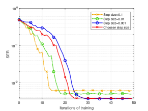
Refer to caption
Figure 6: SER of deep-unfolding NN versus iteration number for different step sizes.

Fig. 7 presents the effects of the number of layers L๐ฟL on the SER performance of the deep-unfolding NN. Increasing the number of layers slows down convergence (as expected) but also affects the residual SER after convergence. As L๐ฟL is increased from 666 to 181818, the residual SER decreases until it reaches a lower bound but then starts to increase. Indeed, as L๐ฟL is further increased, the propagation of gradient errors and the effect of gradient disappearance also become more pronounced.
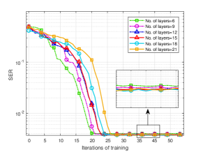
Refer to caption
Figure 7: SER of deep unfolding NN versus different number for layers.

VI-C SER Performance for QPSK Signals

Fig. 8 shows the SER performance versus SNR in downlink MIMO transmission for the following schemes: MMSE-based fully digital GD beamforming algorithm, MMSE-based hybrid GD beamforming algorithm, MMSE-based hybrid OMP beamforming algorithm, MMSE-based hybrid MO beamforming algorithm, MSER-based fully digital GD beamforming algorithm, proposed MSER-based hybrid GD beamforming algorithm, MMSE-based benchmark CNN, MSER-based benchmark CNN and proposed MSER-based deep-unfolding NN. The results show that the proposed MSER-based algorithms significantly outperform the existing MMSE-based algorithms in terms of SER. Moreover, the performance of the proposed deep-unfolding NN approaches that of the MSER-based hybrid GD algorithm, and the gap between their performance decreases with the increase of SNR. The proposed deep-unfolding NN clearly outperforms the benchmark approach; while both algorithms provide much better performance compared to the MMSE-based fully digital algorithm at high SNR.
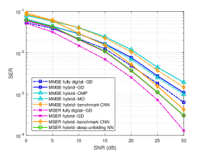
Refer to caption
Figure 8: SER performance versus SNR for the different algorithms (Rr,k=4subscript๐‘…๐‘Ÿ๐‘˜4R_{r,k}=4, D=3๐ท3D=3).

Table I presents the SER versus SNR for the proposed MSER-based deep-unfolding NN, hybrid GD beamforming algorithm and benchmark CNN, where the number of iterations/layers is emphasized for comparison. We find that the proposed deep-unfolding NN requires a smaller number of layers than the black-box CNN to achieve a similar (or better) performance, while a much larger number of iterations is required by the GD algorithm to reach that performance level. Consequently, in the testing stage, the two NN schemes exhibit a much reduced computational complexity compared to the iterative GD scheme (see below).

TABLE I: SER versus SNR.
Hybrid GD Benchmark CNN Deep-unfolding NN
500500500 iterations 171717 layers 151515 layers
SNR = 555 dB 4.11ร—10โˆ’24.11superscript1024.11\times 10^{-2} 5.92ร—10โˆ’25.92superscript1025.92\times 10^{-2} 4.27ร—10โˆ’24.27superscript1024.27\times 10^{-2}
ย SNR = 151515 dB 1.06ร—10โˆ’21.06superscript1021.06\times 10^{-2} 1.51ร—10โˆ’21.51superscript1021.51\times 10^{-2} 1.09ร—10โˆ’21.09superscript1021.09\times 10^{-2}
ย SNR = 252525 dB 1.09ร—10โˆ’31.09superscript1031.09\times 10^{-3} 1.54ร—10โˆ’31.54superscript1031.54\times 10^{-3} 1.11ร—10โˆ’31.11superscript1031.11\times 10^{-3}

Tableย II shows the SER for different configurations of the MIMO system, i.e., different number of users K๐พK and number of receiving RF chains Rr,ksubscript๐‘…๐‘Ÿ๐‘˜R_{r,k}, in the case of SNR = 202020 dB. The percentages of the deep-unfolding NN in the table are calculated via dividing the SER of the iterative GD algorithm by those of the deep-unfolding NN (the percentages in the tables below are the same). The percentages of the benchmark CNN are calculated in the same way. We observe that the performance gap between the proposed deep-unfolding NN and the MSER-based GD algorithm slightly increases with K๐พK. Moreover, the gap between the SER of the general benchmark CNN and that of the deep-unfolding NN becomes larger with K๐พK. This could be the result of increased multi-user interference, which hinders the ability of the NN to learn from the training data. However, the proposed deep-unfolding NN always provides performance close to the MSER-based GD algorithm.

TABLE II: SER for different MIMO system configuration at SNR = 202020 dB.
(K๐พK, Rr,ksubscript๐‘…๐‘Ÿ๐‘˜R_{r,k}) (111, 444) (222, 444) (333, 222) (444, 222)
Hybrid GD 1.15ร—10โˆ’31.15superscript1031.15\!\!\times\!\!10^{-3} 3.64ร—10โˆ’33.64superscript1033.64\!\!\times\!\!10^{-3} 6.83ร—10โˆ’36.83superscript1036.83\!\!\times\!\!10^{-3} 1.56ร—10โˆ’21.56superscript1021.56\!\!\times\!\!10^{-2}
Deep-unfolding NN 98.4398.4398.43%percent\% 97.8597.8597.85%percent\% 97.0797.0797.07%percent\% 95.8695.8695.86%percent\%
Benchmark CNN 73.1473.1473.14%percent\% 70.4870.4870.48%percent\% 68.5268.5268.52%percent\% 65.0265.0265.02%percent\%

Table III shows the SER performance of the NN schemes versus the number of training data samples for SNR = 202020 dB. We observe that the deep-unfolding NN needs much fewer training data samples compared to the benchmark CNN since its structure is developed based on that of the MSER-based GD algorithm.

TABLE III: SER versus the number of training samples for SNR = 202020 dB.
Training samples 500050005000 100001000010000 150001500015000 200002000020000 250002500025000 300003000030000 350003500035000 400004000040000
Benchmark CNN 66.0366.0366.03%percent\% 70.4870.4870.48%percent\% 72.5572.5572.55%percent\% 73.6173.6173.61%percent\% 74.1374.1374.13%percent\% 74.2174.2174.21%percent\% 74.3674.3674.36%percent\% 74.3674.3674.36%percent\%
Training samples 100100100 200200200 300300300 400400400 500500500 600600600 700700700 800800800
Deep-unfolding NN 92.8392.8392.83%percent\% 95.0495.0495.04%percent\% 96.2196.2196.21%percent\% 97.3797.3797.37%percent\% 97.8597.8597.85%percent\% 97.9497.9497.94%percent\% 98.0298.0298.02%percent\% 98.0298.0298.02%percent\%

Fig. 9 illustrates the SER performance versus SNR of the various hybrid AD MIMO transceiver designs in the presence of imperfect CSI. The channel estimation errors are represented by ๐‡k=๐‡ยฏk+ฯƒhโ€‹ฮ”โ€‹๐Šksubscript๐‡๐‘˜subscriptยฏ๐‡๐‘˜subscript๐œŽโ„Žฮ”subscript๐Š๐‘˜\mathbf{H}_{k}=\mathbf{\bar{H}}_{k}+\sigma_{h}\Delta\mathbf{K}_{k}, โˆ€kโˆˆ๐’ฆfor-all๐‘˜๐’ฆ\forall k\in\mathcal{K}, where ๐‡ksubscript๐‡๐‘˜\mathbf{H}_{k} is the true (synthesized) channel matrix, ๐‡ยฏksubscriptยฏ๐‡๐‘˜\mathbf{\bar{H}}_{k} denotes its estimates, and the term ฯƒhโ€‹ฮ”โ€‹๐Šksubscript๐œŽโ„Žฮ”subscript๐Š๐‘˜\sigma_{h}\Delta\mathbf{K}_{k} is the estimation error. In this latter term, ฮ”โ€‹๐Škฮ”subscript๐Š๐‘˜\Delta\mathbf{K}_{k} is a random matrix with zero-mean, unit variance uncorrelated elements following a circular complex Gaussian distribution, while ฯƒh2superscriptsubscript๐œŽโ„Ž2\sigma_{h}^{2} provides the estimation error variance, assumed identical โˆ€kfor-all๐‘˜\forall k for simplicity. We can see that the SER performance degrades with the error variance ฯƒh2superscriptsubscript๐œŽโ„Ž2\sigma_{h}^{2}. Moreover, the best performance is achieved by the proposed deep-unfolding NN, followed by the MSER-based GD beamforming algorithm and the MMSE-based GD beamforming algorithm. These results show that the proposed deep-unfolding NN has stronger robustness against the channel uncertainties compared to the other schemes.
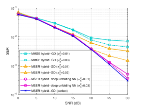
Refer to caption
Figure 9: SER performance of different schemes versus SNR in the presence of imperfect CSI (SNR = 202020 dB).

Fig. 10 illustrates the transfer ability of the proposed schemes, by plotting their SER performance versus SNR for different channel scenarios. Specifically, in this experiment, we first train a network with data based on the considered mmWave channel characteristics, and then transfer the model to the Gaussian channel model. When retraining the model, the parameters of the first 101010 layers are fixed and only the parameters of the remaining layers are trainable. From the result, we can see that the gap between the transferred deep-unfolding NN and the MSER-based hybrid GD algorithm with perfect CSI is much smaller compared to that of the transferred benchmark CNNs under the MSER and MMSE criteria. It shows that the proposed deep-unfolding NN has a better performance in transfer learning as it can significantly apply the knowledge gained from an older scenario and quickly adapt to a new one with less training time.
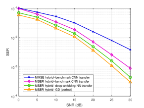
Refer to caption
Figure 10: SER performance of different schemes versus SNR under transfer conditions.

Tableย IV presents the computational complexity of the proposed schemes for different system configurations, as measured by the CPU running time of the training and testing stages. From the results, we can see that the CPU time of both training and testing stages increases with Ntsubscript๐‘๐‘กN_{t} and K๐พK. Clearly, the proposed deep-unfolding NN requires less training time compared to the CNN, which proves that the former structure can effectively accelerate convergence and reduce the training overhead. Since the deep-unfolding NN requires a much smaller number of trainable parameters and the gradients are computed in close-form in the BP, this makes it more efficient compared to the CNN which employs the platform โ€œtensorflowโ€. Moreover, the gap in CPU time between the CNN and the deep-unfolding NN increases with Ntsubscript๐‘๐‘กN_{t} and K๐พK, where the training time is much larger than the testing time. The reason is that there are more complex computations in the training stage but only the FP process in the testing stage.

TABLE IV: CPU running time of the proposed algorithm.
(Ntsubscript๐‘๐‘กN_{t}, K๐พK, Rrsubscript๐‘…๐‘ŸR_{r}) CPU time of training stage (min) CPU time of testing stage (s)
Deep-unfolding NN Benchmark CNN Deep-unfolding NN Benchmark CNN
(646464, 222, 444) 5.355.355.35 8.738.738.73 0.010.010.01 0.010.010.01
(646464, 333, 222) 12.4612.4612.46 21.5821.5821.58 0.010.010.01 0.10.10.1
(128128128, 444, 888) 84.4584.4584.45 130.79130.79130.79 0.070.070.07 0.110.110.11
(128128128, 555, 666) 95.7395.7395.73 200.46200.46200.46 0.100.100.10 0.130.130.13
(128128128, 666, 555) 109.48109.48109.48 242.35242.35242.35 0.140.140.14 0.170.170.17
(128128128, 777, 444) 129.63129.63129.63 295.43295.43295.43 0.170.170.17 0.220.220.22
(128128128, 888, 444) 162.86162.86162.86 360.15360.15360.15 0.240.240.24 0.280.280.28

Table V aims to show the generalization ability of the proposed deep-unfolding NN. To this end, we first train a large-scale network with Nt=128subscript๐‘๐‘ก128N_{t}=128, Rt=32subscript๐‘…๐‘ก32R_{t}=32, Nr=16subscript๐‘๐‘Ÿ16N_{r}=16, Rr=4subscript๐‘…๐‘Ÿ4R_{r}=4, K=8๐พ8K=8, and Dk=3subscript๐ท๐‘˜3D_{k}=3 and then implement it to test the performance of a MIMO system with smaller number of users K๐พK and transmit antennas Ntsubscript๐‘๐‘กN_{t}. From the results, we can see that the performance loss of applying this large-scale network to test the scenarios with smaller K๐พK and Ntsubscript๐‘๐‘กN_{t} is slight, which indicates the strong generalization ability of the proposed deep-unfolding NN.

TABLE V: Generalization ability of the proposed deep-unfolding NN.
Ntsubscript๐‘๐‘กN_{t} K๐พK 888 666 444 222
128128128 98.0498.0498.04%percent\% 98.4598.4598.45%percent\% 98.9398.9398.93%percent\% 99.3799.3799.37%percent\%
646464 โ€” โ€” 96.9496.9496.94%percent\% 97.5297.5297.52%percent\%

VI-D SER Performance for 16-QAM Signals

Fig. 11 presents the SER performance of the different schemes versus SNR in the case of 16-QAM modulation. Similar to the QPSK modulation, the MSER-based algorithms achieve better performance than the MMSE-based algorithms. Meanwhile, the performance of the proposed deep-unfolding NN approaches that of the MSER-based hybrid GD beamforming algorithm although the performance gap between these two schemes decreases with SNR. In addition, we observe that the proposed deep-unfolding NN significantly outperforms the benchmark CNN at lower SNR. Table VI provides the SER values along with the number of the iterations/layers for SNR =25absent25=25 dB. It demonstrates the ability of the deep-unfolding NN to achieve nearly the same performance as the hybrid GD method while significantly reducing computational complexity. The above results show that the proposed deep-unfolding NN still works well for other higher-order modulation schemes.
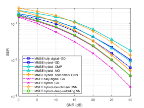
Refer to caption
Figure 11: SER performance of the different schemes versus SNR for 16-QAM signals.
TABLE VI: SER versus the iterations/layers for SNR = 252525 dB.
Hybrid GD Benchmark CNN Deep-unfolding NN
500500500 iterations 171717 layers 151515 layers
ย SNR = 252525 dB 9.8ร—10โˆ’39.8superscript1039.8\times 10^{-3} 1.36ร—10โˆ’21.36superscript1021.36\times 10^{-2} 1.01ร—10โˆ’21.01superscript1021.01\times 10^{-2}

Fig. 12 illustrates the transfer ability of the proposed shemes for 16-QAM signals. We can see that the gap between the deep-unfolding NN and the MSER-based hybrid GD algorithm is much smaller compared to that of the benchmark CNNs for changed channel characteristics. The results show that the proposed deep-unfolding NN has a better performance in transfer learning compared to the benchmark CNNs.
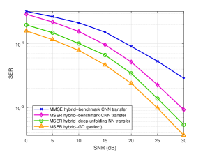
Refer to caption
Figure 12: SER performance of different schemes versus SNR under transfer conditions.

VII Conclusion

In this work, we addressed the problem of hybrid AD transceiver design for massive-MIMO systems based on the MSER criterion. Following the mathematical formulation of the problem as a constrained optimization, we first developed a MSER-based GD iterative algorithm to find stationary points. We then unfolded the GD iterative algorithm into a multi-layer structure and proposed a deep-unfolding NN, where a set of trainable parameters are introduced to reduce the computational complexity and improve the system performance. For the purpose of training, we obtained the relationship linking the gradients between two adjacent layers based on the GCR. The deep-unfolding NN was proposed for both QPSK and M๐‘€M-QAM signal constellations and its convergence was investigated through theoretical analysis; besides, we developed a black-box NN based on a recently proposed approach, for use as a benchmark. Simulation results showed that the proposed deep-unfolding NN provides better SER performance compared to the black-box CNN and approaches the performance of the MSER-based GD iterative algorithm with much lower complexity. Extensions of the deep-unfolding schemes developed in this paper to nonlinear modulation techniques or other types of beamforming algorithms are interesting avenues for future work.

Appendix A GCR in Matrix Form

Based on [39], the general form of the optimization problem can be formulated as

min๐—โกgโ€‹(๐—;๐™)s.t.๐—โˆˆ๐’ฎ,formulae-sequencesubscript๐—๐‘”๐—๐™st๐—๐’ฎ\min\limits_{\mathbf{X}}\ g(\mathbf{X};\mathbf{Z})\quad{\rm s.t.}\ \mathbf{X}\in\mathcal{S},\vspace{-1mm} (49)

where g:โ„‚mร—nโ†’โ„:๐‘”โ†’superscriptโ„‚๐‘š๐‘›โ„g:\mathbb{C}^{m\times n}\rightarrow\mathbb{R} denotes a continuous objective function, ๐—โˆˆโ„‚mร—n๐—superscriptโ„‚๐‘š๐‘›\mathbf{X}\in\mathbb{C}^{m\times n} denotes the variable, ๐’ฎ๐’ฎ\mathcal{S} is the feasible region, and ๐™๐™\mathbf{Z} is the random parameter in the problem. To solve the problem, an iterative algorithm is developed as

๐—t+1=Gtโ€‹(๐—t;๐™),superscript๐—๐‘ก1subscript๐บ๐‘กsuperscript๐—๐‘ก๐™\mathbf{X}^{t+1}=G_{t}(\mathbf{X}^{t};\mathbf{Z}),\vspace{-1mm} (50)

where function Gtโ€‹(โ‹…)subscript๐บ๐‘กโ‹…G_{t}(\cdot) maps the variable ๐—tsuperscript๐—๐‘ก\mathbf{X}^{t} to the variable ๐—t+1superscript๐—๐‘ก1\mathbf{X}^{t+1} in the t๐‘กt-th iteration. To reduce the computational complexity, trainable parameter ๐€๐€\bm{\lambda} is introduced. Since ๐™๐™\mathbf{Z} is a random variable, we need to take the expectation of ๐™๐™\mathbf{Z} and the problem is transformed into

min๐—โก๐”ผ๐™โ€‹{gโ€‹(๐—;๐€,๐™)}s.t.๐—โˆˆ๐’ฎ.formulae-sequencesubscript๐—subscript๐”ผ๐™๐‘”๐—๐€๐™st๐—๐’ฎ\min\limits_{\mathbf{X}}\ \mathbb{E}_{\mathbf{Z}}\{g(\mathbf{X};\bm{\lambda},\mathbf{Z})\}\quad{\rm s.t.}\ \mathbf{X}\in\mathcal{S}.\vspace{-1mm} (51)

A deep-unfolding NN can be developed for the above problem as follows,

๐—l+1=๐’ขlโ€‹(๐—l;๐€l,๐™),superscript๐—๐‘™1subscript๐’ข๐‘™superscript๐—๐‘™superscript๐€๐‘™๐™\mathbf{X}^{l+1}=\mathcal{G}_{l}(\mathbf{X}^{l};\bm{\lambda}^{l},\mathbf{Z}),\vspace{-2mm} (52)

where ๐’ขlโ€‹(โ‹…)subscript๐’ข๐‘™โ‹…\mathcal{G}_{l}(\cdot) denotes the update function of the NN in the l๐‘™l-th layer, ๐—lsuperscript๐—๐‘™\mathbf{X}^{l} and ๐—l+1superscript๐—๐‘™1\mathbf{X}^{l+1} denote the input and output of the l๐‘™l-th layer, respectively, ๐™๐™\mathbf{Z} represents the fixed parameter or input of the NN, and ๐€lsuperscript๐€๐‘™\bm{\lambda}^{l} is the trainable parameter in the l๐‘™l-th layer. For such a NN, in order to train the parameter ๐€lsuperscript๐€๐‘™\bm{\lambda}^{l}, we need to derive the relationship between the gradients of adjacent layers and then calculate the gradient w.r.t. ๐€lsuperscript๐€๐‘™\bm{\lambda}^{l}. To apply the GCR which leads to an expression of the following type

Trโ€‹(๐†l+1โ€‹dโ€‹๐—l+1)=Trโ€‹(๐†l+1โˆ˜๐’ฅโ€‹(๐—l;๐€l,๐™)โ€‹dโ€‹๐—l),Trsuperscript๐†๐‘™1๐‘‘superscript๐—๐‘™1Trsuperscript๐†๐‘™1๐’ฅsuperscript๐—๐‘™superscript๐€๐‘™๐™๐‘‘superscript๐—๐‘™{\rm Tr}\left(\mathbf{G}^{l+1}\,d\mathbf{X}^{l+1}\right)={\rm Tr}\left(\mathbf{G}^{l+1}\circ\mathcal{J}(\mathbf{X}^{l};\bm{\lambda}^{l},\mathbf{Z})\,d\mathbf{X}^{l}\right),\vspace{-1mm} (53)

where ๐†l+1superscript๐†๐‘™1\mathbf{G}^{l+1} and ๐†lsuperscript๐†๐‘™\mathbf{G}^{l} are the gradients w.r.t. ๐—l+1superscript๐—๐‘™1\mathbf{X}^{l+1} and ๐—lsuperscript๐—๐‘™\mathbf{X}^{l}, respectively, ๐’ฅโ€‹(๐—l;๐€l,๐™)๐’ฅsuperscript๐—๐‘™superscript๐€๐‘™๐™\mathcal{J}(\mathbf{X}^{l};\bm{\lambda}^{l},\mathbf{Z}) denotes some matrix functions of ๐—lsuperscript๐—๐‘™\mathbf{X}^{l}, ๐€lsuperscript๐€๐‘™\bm{\lambda}^{l}, and ๐™๐™\mathbf{Z}, which are related to the update function ๐’ขlโ€‹(โ‹…)subscript๐’ข๐‘™โ‹…\mathcal{G}_{l}(\cdot). Then, we obtain the desired gradient relationship as

๐†l=๐†l+1โˆ˜๐’ฅโ€‹(๐—l;๐€l,๐™).superscript๐†๐‘™superscript๐†๐‘™1๐’ฅsuperscript๐—๐‘™superscript๐€๐‘™๐™\mathbf{G}^{l}=\mathbf{G}^{l+1}\circ\mathcal{J}(\mathbf{X}^{l};\bm{\lambda}^{l},\mathbf{Z}).\vspace{-1mm} (54)

In this work, when ๐—๐—\mathbf{X} denotes ๐ksubscript๐๐‘˜\mathbf{P}_{k}, we find that ๐’ฅโ€‹(โ‹…)=๐’ฅ1โ€‹(โ‹…)โˆ˜๐’ฅ2โ€‹(โ‹…)๐’ฅโ‹…subscript๐’ฅ1โ‹…subscript๐’ฅ2โ‹…\mathcal{J}(\cdot)=\mathcal{J}_{1}(\cdot)\circ\mathcal{J}_{2}(\cdot), where ๐’ฅ1โ€‹(โ‹…)=๐„โŸ‚โˆ’bkHโ€‹Bโ€‹(๐œถPkl)Tโ€‹(๐…l)Hโ€‹๐‡kHsubscript๐’ฅ1โ‹…superscript๐„perpendicular-tosuperscriptsubscript๐‘๐‘˜๐ป๐ตsuperscriptsuperscriptsubscript๐œถsubscript๐‘ƒ๐‘˜๐‘™๐‘‡superscriptsuperscript๐…๐‘™๐ปsuperscriptsubscript๐‡๐‘˜๐ป\mathcal{J}_{1}(\cdot)=\mathbf{E}^{\perp}-b_{k}^{H}B(\bm{\alpha}_{P_{k}}^{l})^{T}(\mathbf{F}^{l})^{H}\mathbf{H}_{k}^{H} (๐”kl)Hโ€‹๐–klsuperscriptsuperscriptsubscript๐”๐‘˜๐‘™๐ปsuperscriptsubscript๐–๐‘˜๐‘™(\mathbf{U}_{k}^{l})^{H}\mathbf{W}_{k}^{l} and ๐’ฅ2โ€‹(โ‹…)=๐„subscript๐’ฅ2โ‹…๐„\mathcal{J}_{2}(\cdot)=\mathbf{E}, where ๐„๐„\mathbf{E} is given in Section IV-B.

Appendix B Gradients of Trainable Parameters

According to the update rules in (27)โ€“(30), the gradients w.r.t. the introduced trainable parameters in each layer are acquired as follows, where the index of iteration t๐‘กt is omitted for simplicity.

โˆ‡๐œถPk๐’ซ~el=โˆ’(๐†Pkl+1)Hโˆ˜(โˆ‡๐kH๐’ซ~el)H,โˆ‡๐ŽPk๐’ซ~el=(๐†Pkl+1)H,โˆ‡๐œถฮธF๐’ซ~el=โˆ’(๐†Fl+1)Hโˆ˜jโ€‹๐…โˆ—โˆ˜(โˆ‡๐…๐’ซ~el)H+(๐†Fโˆ—l+1)Hโˆ˜jโ€‹๐…โˆ˜(โˆ‡๐…โˆ—๐’ซ~el)H,โˆ‡๐ŽฮธF๐’ซ~el=(๐†Fl+1)Hโˆ˜jโ€‹๐…โˆ—โˆ’(๐†Fโˆ—l+1)Hโˆ˜jโ€‹๐…,โˆ‡ฯPk๐’ซ~el=1Jโ€‹2โ€‹ฯ€โ€‹(ฯPkl)2โ€‹โˆ‘j=1Jโˆ‘i=1Dkeโˆ’|bยฏi,kqj|22โ€‹(ฯPkl)2โ€‹(1โˆ’|bยฏi,kqj|22โ€‹(ฯPkl)2)โ€‹๐†Pkl+1โˆ˜(๐œถPkl)Tโ€‹๐…Hโ€‹๐‡kHโ€‹๐”kHโ€‹๐ฐi,k.\begin{split}&\!\!\nabla_{\bm{\alpha}_{P_{k}}}\tilde{\mathcal{P}}_{e}^{l}=-(\mathbf{G}_{P_{k}}^{l+1})^{H}\circ(\nabla_{\mathbf{P}_{k}^{H}}\tilde{\mathcal{P}}_{e}^{l})^{H},\nabla_{\mathbf{O}_{P_{k}}}\tilde{\mathcal{P}}_{e}^{l}=(\mathbf{G}_{P_{k}}^{l+1})^{H},\\ &\!\!\nabla_{\bm{\alpha}_{\theta_{F}}}\tilde{\mathcal{P}}_{e}^{l}=-(\mathbf{G}_{\!F}^{\!l\!+\!1})^{\!H}\!\circ\!j\mathbf{F}^{*}\!\circ\!(\nabla_{\!\mathbf{F}}\tilde{\mathcal{P}}_{\!\!e}^{l})^{\!H}\!+\!(\mathbf{G}_{\!F^{\!*}}^{\!l\!+\!1})^{\!H}\!\circ\!j\mathbf{F}\!\circ\!(\nabla_{\!\mathbf{F}^{*}}\!\tilde{\mathcal{P}}_{\!\!e}^{l})^{\!H},\\ &\!\!\nabla_{\mathbf{O}_{\theta_{F}}}\tilde{\mathcal{P}}_{e}^{l}=(\mathbf{G}_{F}^{l+1})^{H}\circ j\mathbf{F}^{*}-(\mathbf{G}_{F^{*}}^{l+1})^{H}\circ j\mathbf{F},\\ &\!\nabla_{\rho_{P_{k}}}\tilde{\mathcal{P}}_{e}^{l}=\frac{1}{J\sqrt{2\pi}(\rho_{P_{k}}^{l})^{2}}\sum\limits_{{j}=1}^{J}\sum\limits_{i=1}^{D_{k}}e^{-\frac{|\bar{b}^{{q_{j}}}_{i,k}|^{2}}{2(\rho_{P_{k}}^{l})^{2}}}\!\Big{(}1-\frac{|\bar{b}^{{q_{j}}}_{i,k}|^{2}}{2(\rho_{P_{k}}^{l})^{2}}\Big{)}\mathbf{G}_{P_{k}}^{l+1}\\ &\qquad\quad\circ(\bm{\alpha}_{P_{k}}^{l})^{T}\mathbf{F}^{H}\mathbf{H}_{k}^{H}\mathbf{U}_{k}^{H}\mathbf{w}_{i,k}.\end{split} (55)

References

  • [1] Z. Pi and F. Khan, โ€œAn introduction to millimeter-wave mobile broadband systems,โ€ IEEE Commun. Mag., vol. 49, no. 6, pp. 101-108, Jun. 2011.
  • [2] T. S. Rappaport, S. Sun, R. Mayzus, H. Zhao, Y. Azar, K. Wang, G. N. Wong, J. K. Schulz, M. Samimi, and F. Gutierrez, โ€œMillimeter wave mobile communications for 5G cellular: It will work!โ€ IEEE Access, vol. 1, pp. 335-349, May 2013.
  • [3] T. Kim, J. Park, J.-Y. Seol, S. Jeong, J. Cho, and W. Roh, โ€œTens of Gbps support with mmWave beamforming systems for next generation communications,โ€ in IEEE Global Communications Conference (GLOBECOM), Dec. 2013, pp. 3685-3690.
  • [4] X. Zhang, A. F. Molisch, and S.-Y. Kung, โ€œVariable-phase-shift-based RF-baseband codesign for MIMO antenna selection,โ€ IEEE Trans. Signal Process., vol. 53, no. 11, pp. 4091-4103, Oct. 2005.
  • [5] P. Sudarshan, N. B. Mehta, A. F. Molisch, and J. Zhang, โ€œChannel statistics-based RF pre-processing with antenna selection,โ€ IEEE Trans. Wireless Commun., vol. 5, no. 12, pp. 3501-3511, Dec. 2006.
  • [6] O. E. Ayach, S. Rajagopal, S. Abu-Surra, Z. Pi, and R. W. Heath, โ€œSpatially sparse precoding in millimeter wave MIMO systems,โ€ IEEE Trans. Wireless Commun., vol. 13, no. 3, pp. 1499-1513, Mar. 2014.
  • [7] F. Sohrabi and W. Yu, โ€œHybrid digital and analog beamforming design for large-scale antenna arrays,โ€ IEEE J. Sel. Topics Signal Process., vol. 10, no. 3, pp. 501-513, Apr. 2016.
  • [8] M. Kim and Y. H. Lee, โ€œMSE-based hybrid RF/baseband processing for millimeter-wave communication systems in MIMO interference channels,โ€ IEEE Trans. Veh. Technol., vol. 64, no. 6, pp. 2714-2720, Jun. 2015.
  • [9] D. H. N. Nguyen, L. B. Le, T. Le-Ngoc, and R. W. Heath, โ€œHybrid MMSE precoding and combining designs for mmWave multiuser systems,โ€ IEEE Access, vol. 5, pp. 19167-19181, 2017.
  • [10] D. H. N. Nguyen, L. B. Le, and T. Le-Ngoc, โ€œHybrid MMSE precoding for mmWave multiuser MIMO systems,โ€ in IEEE Int. Conf. on Communications (ICC), May 2016, pp. 1-6.
  • [11] X. Yu, J. Shen, J. Zhang, and K. B. Letaief, โ€œAlternating minimization algorithms for hybrid precoding in millimeter wave MIMO systems,โ€ IEEE J. Sel. Topics Signal Process., vol. 10, no. 3, pp. 485-500, Apr. 2016.
  • [12] S. He, J. Wang, Y. Huang, B. Ottersten, and W. Hong, โ€œCodebook-based hybrid precoding for millimeter wave multiuser systems,โ€ IEEE Trans. Signal Process., vol. 65, no. 20, pp. 5289-5304, Oct. 2017.
  • [13] J. Cong, X. Li, and Y. Zhu, โ€œHybrid precoding for multi-user mmWave systems based on MMSE criterion,โ€ in 23rd Asia-Pacific Conference on Communications (APCC), Dec. 2017, pp. 1-5.
  • [14] T. Lin, J. Cong, Y. Zhu, J. Zhang, and K. Ben Letaief, โ€œHybrid beamforming for millimeter wave systems using the MMSE criterion,โ€ IEEE Trans. Commun., vol. 67, no. 5, pp. 3693-3708, May 2019.
  • [15] Y. Cai and R. C. de Lamare, โ€œAdaptive linear minimum BER reduced-rank interference suppression algorithms based on joint and iterative optimization of filters,โ€ IEEE Commun. Lett., vol. 17, no. 4, pp. 633-636, Apr. 2013.
  • [16] Y. Cai, R. C. de Lamare, B. Champagne, B. Qin, and M. Zhao, โ€œAdaptive reduced-rank receive processing based on minimum symbol-error-rate criterion for large-scale multiple-antenna systems,โ€ IEEE Trans. Commun., vol. 63, no. 11, pp. 4185-4201, Nov. 2015.
  • [17] M. Shao, Q. Li, and W. Ma, โ€œOne-bit massive MIMO precoding via a minimum symbol-error probability design,โ€ in IEEE International Conference on Acoustics, Speech and Signal Processing (ICASSP), Apr. 2018, pp. 3579-3583.
  • [18] K. L. Law and C. Masouros, โ€œSymbol error rate minimization precoding for interference exploitation,โ€ IEEE Trans. Commun., vol. 66, no. 11, pp. 5718-5731, Nov. 2018.
  • [19] H. D. Nguyen, R. Zhang, and S. Sun, โ€œImproper signaling for symbol error rate minimization in K๐พK-user interference channel,โ€ IEEE Trans. Commun., vol. 63, no. 3, pp. 857-869, Mar. 2015.
  • [20] T. Oโ€™Shea and J. Hoydis, โ€œAn introduction to deep learning for the physical layer,โ€ IEEE Trans. Cogn. Commun. Netw., vol. 3, no. 4, pp. 563-575, Dec. 2017.
  • [21] S. Dรถrner, S. Cammerer, J. Hoydis, and S. T. Brink, โ€œDeep learning based communication over the air,โ€ IEEE J. Sel. Topics Signal Process., vol. 12, no. 1, pp. 132-143, Feb. 2018.
  • [22] P. Dong, H. Zhang, and G. Y. Li, โ€œFramework on Deep Learning-Based Joint Hybrid Processing for mmWave Massive MIMO Systems,โ€ IEEE Access, vol. 8, pp. 106023-106035, 2020.
  • [23] D. Neumann, T. Wiese, and W. Utschick, โ€œLearning the MMSE channel estimator,โ€ IEEE Trans. Signal Process., vol. 66, no. 11, pp. 2905-2917, Jun. 2018.
  • [24] H. Sun, X. Chen, Q. Shi, M. Hong, X. Fu, and N. D. Sidiropoulos, โ€œLearning to optimize: Training deep neural networks for interference management,โ€ IEEE Trans. Signal Process., vol. 66, no. 20, pp. 5438-5453, Oct. 2018.
  • [25] W. Lee, M. Kim, and D. Cho, โ€œDeep power control: Transmit power control scheme based on convolutional neural network,โ€ IEEE Commun. Lett., vol. 22, no. 6, pp. 1276-1279, Jun. 2018.
  • [26] F. Liang, C. Shen, W. Yu, and F. Wu, โ€œTowards optimal power control via ensembling deep neural networks,โ€ IEEE Trans. Commun., vol. 68, no. 3, pp. 1760-1776, Mar. 2020.
  • [27] A. M. Elbir and K. V. Mishra, โ€œDeep learning design for joint antenna selection and hybrid beamforming in massive MIMO,โ€ in IEEE International Symposium on Antennas and Propagation and USNC-URSI Radio Science Meeting, Jul. 2019, pp. 1585-1586.
  • [28] X. Li and A. Alkhateeb, โ€œDeep learning for direct hybrid precoding in millimeter wave massive MIMO systems,โ€ in 53rd Asilomar Conference on Signals, Systems, and Computers, Nov. 2019, pp. 800-805.
  • [29] C. Sidharth, S. M. Hiremath, and S. K. Patra, โ€œDeep learning based hybrid precoding for mmWave massive MIMO system using comcepNet,โ€ in International Conference on Communication and Signal Processing (ICCSP), Jul. 2020, pp. 1317-1321.
  • [30] J. R. Hershey, J. L. Roux, and F. Weninger, โ€œDeep unfolding: Model-based inspiration of novel deep architectures,โ€ arXiv preprint arXiv:1409.2574, 2014.
  • [31] V. Corlay, J. J. Boutros, P. Ciblat, and L. Brunel, โ€œMultilevel MIMO detection with deep learning,โ€ in 52nd Asilomar Conference on Signals, Systems, and Computers, Oct. 2018, pp. 1805-1809.
  • [32] N. Samuel, T. Diskin, and A. Wiesel, โ€œLearning to detect,โ€ IEEE Trans. Signal Process., vol. 67, no. 10, pp. 2554-2564, May 2019.
  • [33] W. Xu, Z. Wu, Y. Ueng, X. You, and C. Zhang, โ€œImproved polar decoder based on deep learning,โ€ in IEEE International Workshop on Signal Processing Systems (SiPS), Oct. 2017, pp. 1-6.
  • [34] W. Xu, X. You, C. Zhang, and Y. Beโ€™ery, โ€œPolar decoding on sparse graphs with deep learning,โ€ in 52nd Asilomar Conference on Signals, Systems, and Computers, Oct. 2018, pp. 599-603.
  • [35] D. Ito, S. Takabe, and T. Wadayama, โ€œTrainable ISTA for sparse signal recovery,โ€ IEEE Trans. Signal Process., vol. 67, no. 12, pp. 3113-3125, Jun. 2019.
  • [36] A. Balatsoukas-Stimming, O. Castaรฑeda, S. Jacobsson, G. Durisi, and C. Studer, โ€œNeural-network optimized 1-bit precoding for massive MU-MIMO,โ€ in IEEE 20th International Workshop on Signal Processing Advances in Wireless Communications (SPAWC), Jul. 2019, pp. 1-5.
  • [37] Y. He, H. He, C. -K. Wen, and S. Jin, โ€œModel-driven deep learning for massive multiuser MIMO constant envelope precoding,โ€ IEEE Wireless Commun. Lett., vol. 9, no. 11, pp. 1835-1839, Nov. 2020.
  • [38] H. He, M. Zhang, S. Jin, C. -K. Wen, and G. Y. Li, โ€œModel-driven deep learning for massive MU-MIMO with finite-alphabet precoding,โ€ IEEE Commun. Lett., vol. 24, no. 10, pp. 2216-2220, Oct. 2020.
  • [39] Q. Hu, Y. Cai, Q. Shi, K. Xu, G. Yu, and Z. Ding, โ€œIterative algorithm induced deep-unfolding neural networks: Precoding design for multiuser MIMO systems,โ€ IEEE Trans. Wireless Commun., vol. 20, no. 2, pp. 1394-1410, Feb. 2021.
  • [40] S. Chen, A. K. Samingan, B. Mulgrew, and L. Hanzo, โ€œAdaptive minimum-BER linear multiuser detection for DS-CDMA signals in multipath channels,โ€ IEEE Trans. Signal Process., vol. 49, no. 6, pp. 1240-1247, Jun. 2001.
  • [41] S. Chen, A. Livingstone, H. -Q. Du, and L. Hanzo, โ€œAdaptive minimum symbol error rate beamforming assisted detection for quadrature amplitude modulation,โ€ IEEE Trans. Wireless Commun., vol. 7, no. 4, pp. 1140-1145, Apr. 2008.
  • [42] X. Zhang, Matrix Analysis and Applications, U.K., Cambridge Univ. Press, 2017.