Uncertainty-Aware Machine Translation Evaluation

Abstract

Several neural-based metrics have been recently proposed to evaluate machine translation quality. However, all of them resort to point estimates, which provide limited information at segment level. This is made worse as they are trained on noisy, biased and scarce human judgements, often resulting in unreliable quality predictions. In this paper, we introduce uncertainty-aware MT evaluation and analyze the trustworthiness of the predicted quality. We combine the Comet framework with two uncertainty estimation methods, Monte Carlo dropout and deep ensembles, to obtain quality scores along with confidence intervals. We compare the performance of our uncertainty-aware MT evaluation methods across multiple language pairs from the QT21 dataset and the WMT20 metrics task, augmented with MQM annotations. We experiment with varying numbers of references and further discuss the usefulness of uncertainty-aware quality estimation (without references) to flag possibly critical translation mistakes.

1 Introduction

MT	DA	Comet	UA-Comet
Она сказала,	-0.815	0.586	0.149
’Это не собирается			[-0.92, 1.22]
работать.
Gloss: “She said, ‘that’s not willing to work”
Она сказала:	0.768	1.047	1.023
«Это не сработает.			[0.673, 1.374]
Gloss: “She said, «That will not work”

Table 1: Example of uncertainty-aware MT evaluation for a sentence in the WMT20 dataset. Shown are two Russian translations of the same English source “She said, ‘That’s not going to work.” with reference “Она сказала: “Не получится.” For the first sentence, Comet provides a point estimate (in red) that overestimates quality, as compared to a human direct assessment (DA), while our UA-Comet (in green) returns a large 95% confidence interval which contains the DA value. For the second sentence UA-Comet is confident and returns a narrow 95% confidence interval.

Evaluation of machine translation (MT) quality is a key problem with several use cases: it is needed to compare and select MT systems, to decide on the fly whether a translation is ready for publication or needs to be post-edited by a human, and more generally to track progress in the field (Specia et al., 2018; Mathur et al., 2020). Even when reference translations are available, the increasing quality of neural MT systems has made traditional lexical-based metrics such as Bleu Papineni et al. (2002) or chrF Popović (2015) insufficient to distinguish the best systems. This fostered a line of work on neural-based metrics, with recent proposals such as Bleurt Sellam et al. (2020), Comet Rei et al. (2020a) and Prism Thompson and Post (2020a). Metrics for quality estimation (QE; when references are not available) have also been developed as part of OpenKiwi Kepler et al. (2019) and TransQuest (Ranasinghe et al., 2020).

While the metrics above have enjoyed some success in system-level evaluation – where the goal is to compare different systems – their segment-level quality scores are often unreliable for practical use. They all share the limitation that their output is a single point estimate – they do not provide any uncertainty information, such as confidence intervals, with their quality predictions. This is an important limitation: often, complex or out-of-domain sentences receive quality estimates that are far from their true quality (as illustrated in Table 1). This may lead to translations with critical mistakes being undetected, and hinders worst-case performance analysis of MT systems.

In this paper, we propose a simple and effective method to obtain uncertainty-aware quality/metric estimation systems, by representing quality as a distribution, rather than a single value. To this end, we make use of and compare two well-studied techniques for uncertainty estimation: Monte Carlo (MC) dropout Gal and Ghahramani (2016) and deep ensembles Lakshminarayanan et al. (2017). In both cases, our method is agnostic to the particular metric estimation system, as long as it can be ensembled or perturbed. In our experiments we use Comet Rei et al. (2020a), and we call our uncertainty-aware version UA-Comet.

Our method allows using the same system with a varying number of references. We show that confidence intervals tend to shrink as more references are added, which matches the intuition that MT evaluation systems should become more confident as they have access to more information.

We evaluate our approach using data from the WMT20 metrics task (Mathur et al., 2020), including its recent extension with Google MQM annotations (Freitag et al., 2021), and the QT21 dataset Specia et al. (2017). The results show that our uncertainty-aware systems exhibit better calibration with respect to human direct assessments (DA; Graham et al. 2013), multi-dimensional quality metric scores (MQM; Lommel et al. 2014), and human translation error rates (HTER; Snover et al. 2006) than a simple baseline, while their average quality scores achieve similar or better correlation than the vanilla Comet system. Finally, we illustrate a potential quality estimation use case enabled by our approach: automatically detecting low-quality translations with a risk-based criterion.

2 Related Work

Automatic MT evaluation

Reference-based approaches for MT evaluation include traditional metrics such as Bleu Papineni et al. (2002) and Meteor Denkowski and Lavie (2014), as well as recently proposed Bleurt Sellam et al. (2020), BERTScore Zhang et al. (2020), Prism Thompson and Post (2020a) and Comet Rei et al. (2020a). Approaches that do not make use of human references are generally referred to as QE systems Specia et al. (2018); Kepler et al. (2019); Ranasinghe et al. (2020). Our proposed approach augments reference-based approaches and enables a single system that can be used with multiple references, with the added advantage of providing uncertainty information. To the best of our knowledge, predictive uncertainty in QE has been approached only with Gaussian processes Beck et al. (2016), which are not competitive or easy to integrate with current neural architectures.

Confidence estimation in MT

A related line of work is confidence estimation of sentence-level MT outputs Blatz et al. (2004); Quirk (2004); Wang et al. (2019). The work that relates the most with ours is the one by Fomicheva et al. (2020), who propose an unsupervised glass-box approach to QE, extracting uncertainty-related features from the MT system via MC dropout. They show that the more confident the decoder (as measured by the lower variance of its output), the higher the quality of the MT output. Our work builds upon this perspective to propose uncertainty estimation of the QE systems themselves, rather than uncertainty of MT.

Performance prediction in NLP

A related problem is that of predicting the performance of an NLP system without having to train it (Xia et al., 2020). Recent approaches perform such predictions by adding confidence intervals (Ye et al., 2021) and measuring calibration error. We take inspiration from these works to improve the calibration of our methods Guo et al. (2017); Desai and Durrett (2020) and to evaluate how good our uncertainty estimates are with a suite of performance indicators.

Uncertainty estimation

Overall the concepts and methods of uncertainty quantification Huellermeier and Waegeman (2021) have been widely explored and compared for many different tasks, including MT Ott et al. (2018). Uncertainty estimation in neural networks has traditionally been approached with Bayesian methods, replacing point estimates of weights with probability distributions Mackay (1992); Graves (2011); Welling and Teh (2011); Tran et al. (2019). However, Bayesian neural networks are costly, and in order to avoid high training costs, various approximations come in handy. Model ensembling Dietterich (2000); Garmash and Monz (2016); McClure and Kriegeskorte (2017); Lakshminarayanan et al. (2017); Pearce et al. (2020); Jain et al. (2020) is a commonly used approach, which employs an ensemble of neural networks to obtain multiple point predictions and then uses their empirical variance as an approximate measure of uncertainty. Its main disadvantage is the need to train multiple models. An alternative is MC dropout (Gal and Ghahramani, 2016), which builds upon dropout regularization (Srivastava et al., 2014) but uses it at test time, by performing several stochastic forward passes through the network and computing mean and variance of the resulting outputs as a proxy for the model’s uncertainty. Our work applies and compares the last two techniques to MT evaluation. Note that more elaborate approaches have been proposed to address uncertainty quantification on classification tasks, including calibration approaches Guo et al. (2017); Kuleshov et al. (2018a), the use of Dirichlet distributions Sensoy et al. (2018); Malinin and Gales (2018); Charpentier et al. (2020) and entropy measures Smith and Gal (2018). However, uncertainty in MT evaluation is a regression task which is so far largely overlooked in terms of predictive uncertainty. Our paper can be seen as a first step towards uncertainty-aware MT evaluation models.

3 Uncertainty-Aware MT Evaluation

3.1 Problem definition

Typical MT evaluation systems take as input a tuple $\langle s,t,\mathcal{R}\rangle$, where $s$ is source text, $t$ is machine translated text, and $\mathcal{R}=\{r_{1},\ldots,r_{|\mathcal{R}|}\}$ is a (possibly empty) set of reference translations. Their goal is to predict an automatic score $\hat{q}\in\mathbb{R}$ which assesses the quality of the translation. Supervised systems such as Comet or Bleurt are trained to approximate ground truth scores $q^{*}$ obtained from human annotations, such as DA, MQM and HTER. In this paper, we assume that $q^{*}$ is a continuous real-valued score, but the main ideas extend to the case where $q^{*}$ are discrete classes or quality bins.

3.2 Sources of uncertainty

There are several challenges with learning MT evaluation systems:

1. Noisy scores. The human-generated scores $q^{*}$ are not always reliable and often suffer from high variability, exhibiting low inter-annotator agreement. This problem can be mitigated by averaging over a sufficient number of references, but this brings considerable annotation costs Freitag et al. (2021); Mathur et al. (2020).

2. Noisy or insufficient references. The references $\mathcal{R}$ do not always have good quality, and their sparsity (small $|\mathcal{R}|$) is often insufficient to represent the space of possible correct translations well Freitag et al. (2020). An extreme case is when there are no references ($\mathcal{R}=\varnothing$), a problem known as “QE as a metric.”

3. Complex translations. Correct translations are often non-literal, and it may be hard for an automatic system to grasp the semantic relation between the translated sentence and the references, as they may be confused with hallucinations.

4. Out-of-domain text. The text where the MT evaluation system is run may belong to a different domain from the one it was trained on.

The first two points can be seen as aleatoric uncertainty (noise in the input or output data), whereas the last two are instances of epistemic uncertainty, reflecting the limited knowledge of the model Hora (1996); Kiureghian and Ditlevsen (2009). Unfortunately, these uncertainties add up. To cope with the different sources of uncertainty, we treat the quality score $Q$ as a random variable and predict a distribution $\hat{p}_{Q}(q)$, as opposed to a point estimate $\hat{q}$. This way, we obtain an uncertainty-aware system, which can return a peaked distribution when it is confident about its quality estimate, or a flatter distribution in cases where it is more uncertain. This allows, among other things, managing the risk of treating a translation as good quality when it is not (see §5.4). When estimating quality on the fly without references, knowing the system’s confidence in the quality of the produced translations might help obtain informative worst-case indicators on whether a human post-edit is required, e.g. by evaluating the cumulative distribution function $\hat{F}_{Q}(\chi)=\int_{-\infty}^{\chi}\hat{p}_{Q}(q)dq$ which quantifies the translation risk, i.e., the probability of a translation being below a quality threshold $\chi$. Moreover, having access to such distributions of quality estimates can be beneficial when deciding if a system outperforms another with some level of confidence.

3.3 Uncertainty and confidence intervals

To obtain $\hat{p}_{Q}(q)$, our approach builds upon a vanilla MT evaluation system $h$ (such as Comet) that produces point estimates $\hat{q}=h(\langle s,t,\mathcal{R}\rangle)$, and augments it to produce uncertainty estimates. Our approach is completely agnostic about the system $h$, as long as it can be ensembled or perturbed.

The first step is to use $h$ to produce a set $\mathcal{Q}=\{\hat{q}_{1},\ldots,\hat{q}_{N}\}$ of quality scores for a given input $\langle s,t,\mathcal{R}\rangle$, which will be interpreted as a sample from $\hat{p}_{Q}(q)$. For this, we experiment with two methods: MC dropout (Gal and Ghahramani, 2016), which obtains $\mathcal{Q}$ by running $N$ stochastic forward-passes on $h$ with units dropped out with a given probability; and deep ensembles (Lakshminarayanan et al., 2017), in which $N$ separate models are trained with different random initializations and then run in parallel to obtain $\mathcal{Q}$. While both methods have shown to be effective in several tasks (Fomicheva et al., 2020; Malinin and Gales, 2021), MC dropout is usually more convenient (because only one model is required), but generally requires many more samples for good performance (larger $N$) compared to deep ensembles.

The second step is to use the resulting set $\mathcal{Q}$ to represent model’s uncertainty. One way of representing uncertainty is through confidence intervals, that is, given a desired confidence level $\gamma\in[0,1]$ (e.g. $\gamma=0.95$), specifying the smallest possible quality interval $I(\gamma)=[q_{\min}(\gamma),q_{\max}(\gamma)]$ such that $P(q\in I(\gamma))=\int_{q_{\min}}^{q_{\max}}\hat{p}_{Q}(q)dq\geq\gamma$. There are two possible strategies to obtain such intervals: a parametric approach, which parametrizes the distribution $\hat{p}_{Q}(q)$, produces estimates of its parameters by fitting the distribution on $\mathcal{Q}$, and uses them to compute confidence intervals at arbitrary levels $\gamma$; and a non-parametric approach, which bypasses the estimation of $\hat{p}_{Q}(q)$ and focuses on estimating its quantiles for the desired values of $\gamma$ directly from $\mathcal{Q}$. In this paper, we opted for a simple parametric Gaussian approach, which worked well in practice and seemed to fit our data well (see Figure 3 in App. B). However, we did experiment with a non-parametric bootstrapping technique using the percentile method (Efron, 1979; Johnson, 2001; Ye et al., 2021), which we report in App. E.

In our approach, we treat $\mathcal{Q}$ as a sample drawn from a Gaussian distribution, $\hat{p}_{Q}(q)=\mathcal{N}(q;\hat{\mu},\hat{\sigma}^{2})$, and estimate the parameters $\hat{\mu}$ and $\hat{\sigma}^{2}$ as the sample mean and variance, respectively. Once $\hat{p}_{Q}(q)$ is fit to $\mathcal{Q}$, the confidence intervals $I(\gamma)=[q_{\min}(\gamma),q_{\max}(\gamma)]$ can be estimated at the desired level of confidence $\gamma$, using the probit (quantile) function $\mathrm{probit}(p)=\sqrt{2}\mathrm{erf}^{-1}(2p-1)$ (where $\mathrm{erf}$ is the error function):

$$q_{\min}(\gamma) =\hat{\mu}-\hat{\sigma}\mathrm{probit}((1+\gamma)/2)$$

$$q_{\max}(\gamma) =\hat{\mu}+\hat{\sigma}\mathrm{probit}((1+\gamma)/2).$$ (1)

3.4 MT evaluation with multi-references

As our framework can model uncertainty, it is interesting to consider the case where the number of available references $\mathcal{R}$ may vary. Intuitively, we expect the uncertainty to decrease when the model observes more references. Specifically, relying on a single reference might prove problematic, since even human generated references can be noisy and prone to errors. Additionally, for source sentences with multiple and diverse valid translations, relying on a single reference might result in potential underestimation of the quality of valid MT hypotheses. For the above reasons, additional references, even if they are paraphrased versions of the originals Freitag et al. (2020), can help obtain better evaluations of the MT systems’ outputs.

As a result, relying on human-generated references can be a constraint in terms of learning and predicting accurate quality estimates for adequately diverse data Sun et al. (2020). We thus want to assess the impact of additional references (both independently generated and paraphrased) on the estimated confidence intervals.

Even though our approach works with any underlying MT evaluation system $h$ which produces point estimates, most existing systems cannot seamlessly handle a varying number of references or no references without architecture modifications. For example, Comet originally receives exactly one reference as input to predict the quality of a $\langle s,t\rangle$ pair. We take the following approach to handle a varying number of references ($|\mathcal{R}|>1$): we obtain a set of $N$ quality predictions for each available reference, $r\in\mathcal{R}$, for a given $\langle s,t\rangle$ pair, resulting in a set of $N\times|\mathcal{R}|$ quality predictions. We then compute the pointwise average across the $|\mathcal{R}|$ dimension, leading to $N$ quality scores $\mathcal{Q}=\{\hat{q}_{1},\ldots,\hat{q}_{N}\}$ that aggregate information from all the $|\mathcal{R}|$ references. We can then apply the same approach as described earlier. Intuitively, the averaging operation should reduce variance in the quality scores, which would result in narrower confidence intervals as $|\mathcal{R}|$ increases. We validate this hypothesis in our experiments in §5.4.

3.5 Post-calibration

In our initial experiments, we observed that the magnitude of the predicted variance $\hat{\sigma}^{2}$ depends significantly on several hyperparameters, such as the choice of dropout value, number of samples, and language pair. In classification tasks, a similar phenomenon has been reported by Malinin and Gales (2021), who recommended combining these methods with temperature calibration Platt (1999) to adjust uncertainties and obtain more reliable confidence intervals. For regression tasks – our case of interest – Kuleshov et al. (2018b) also point out the importance of post-calibration. Since temperature scaling is only applicable in classification, they propose an isotonic regression technique instead Niculescu-Mizil and Caruana (2005). We found that we can obtain highly calibrated uncertainty estimates in a much simpler way, by learning an affine transformation $\sigma^{2}\mapsto\sigma^{2}_{\mathrm{calib}}=\alpha\sigma^{2}+\beta$, where $\alpha$ and $\beta$ are scalars, tuned to minimize the calibration error (see Eq. 2–3) on a validation set. We use the tuned $\sigma_{\mathrm{calib}}$ in our experiments (§5), and show the improvement on ECE for different confidence levels with $\sigma_{\mathrm{calib}}$ in Figure 1.

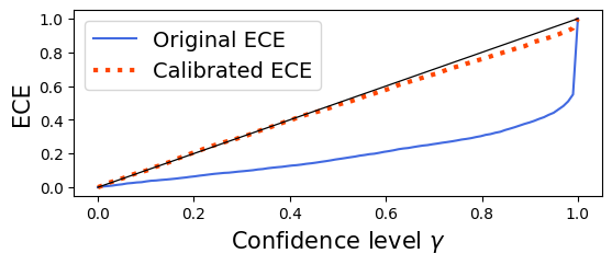
Figure 1: Calibration for En-De language pair. Continuous (blue) line is ECE pre-calibration and dotted (orange) line corresponds to ECE post-calibration.

4 Evaluating Uncertainty

Having described our framework, we now turn to the problem of verifying the effectiveness and informativeness of the proposed uncertainty quantification method. Two crucial aspects to take into account when evaluating uncertainty-aware systems are: (i) the system should not harm the predictive accuracy compared to a system without uncertainty and (ii) the uncertainty estimate should reflect the failure probability of the system well, meaning that the system “knows when it does not know.” In what follows, we assume a test or validation set $\mathcal{D}=\{\langle s_{j},t_{j},\mathcal{R}_{j},q_{j}^{*}\rangle\}_{j=1}^{|\mathcal{D}|}$, consisting of examples together with their ground truth quality scores.

Calibration Error

One way of understanding if models can be trusted is analyzing whether they are calibrated Raftery et al. (2005); Jiang et al. (2011); Kendall and Gal (2017), that is, if the confidence estimates of its predictions are aligned with the empirical likelihoods Guo et al. (2017). In classification tasks, this is assessed by the expected calibration error (ECE; Naeini et al. 2015), which has been generalized to regression by Kuleshov et al. (2018b). It is defined as:

$$\mathrm{ECE} =\frac{1}{M}\sum_{b=1}^{M}|\mathrm{acc}(\gamma_{b})-\gamma_{b}|,$$ (2)

where each $b$ is a bin representing a confidence level $\gamma_{b}$, and $\mathrm{acc}(\gamma_{b})$ is the fraction of times the ground truth $q^{*}$ falls inside the confidence interval $I(\gamma_{b})$:

$$\mathrm{acc}(\gamma_{b})=\frac{1}{|\mathcal{D}|}\sum_{\langle s,t,\mathcal{R},q^{*}\rangle\in\mathcal{D}}\mathds{1}(q^{*}\in I(\gamma_{b})).$$ (3)

We use this metric with $M=100$.

Negative log-likelihood

To evaluate parametric methods that represent the full distribution $\hat{p}_{Q}(q)$, we can use a single metric that captures both accuracy and uncertainty, the average negative log-likelihood of the ground truth quality scores according to the model:

$$\mathrm{NLL}=-\frac{1}{|\mathcal{D}|}\sum_{\langle s,t,\mathcal{R},q^{*}\rangle\in\mathcal{D}}\log\hat{p}(q^{*}\mid\langle s,t,\mathcal{R}\rangle).$$ (4)

This metric penalizes predictions that are accurate but have high uncertainty (since they will become flat distributions with low probability everywhere), and even more severely incorrect predictions with high confidence (as they will be peaked in the wrong location), but is more forgiving to predictions that are inaccurate but have high uncertainty.

Sharpness

The metrics above do not sufficiently account for how “tight” the uncertainty interval is around the predicted value, and thus might generally favour predictors that produce wide and uninformative confidence intervals. To guarantee useful uncertainty estimation, confidence intervals should not only be calibrated, but also sharp. We measure sharpness using the predicted variance $\hat{\sigma}^{2}$, as defined in Kuleshov et al. (2018b):

$$\mathrm{sha}(\hat{p}_{Q})=\frac{1}{|\mathcal{D}|}\sum_{\langle s,t,\mathcal{R}\rangle\in\mathcal{D}}\hat{\sigma}^{2}.$$ (5)

Pearson correlations

As shown by Ashukha et al. (2020), NLL and ECE alone might not be enough to evaluate uncertainty-aware systems. Therefore, we complement the indicators above with two Pearson correlations involving the system’s predictions and the ground truth quality scores coming from human judgements. The first, which we call the predictive Pearson score (PPS), is useful to assess the predictive accuracy of the system, regardless of the uncertainty estimate – it is the Pearson correlation $r(q^{*},\hat{\mu})$ between the ground truth quality scores $q^{*}$ and the average system predictions $\hat{\mu}$ in the dataset $\mathcal{D}$ (for the baseline point estimate system, we use $\hat{q}$ instead of $\hat{\mu}$). We expect this score to be similar to the baseline or slightly better due to the ensemble effect. The second is the uncertainty Pearson score (UPS) $r(|q^{*}-\hat{\mu}|,\hat{\sigma})$, which measures the alignment between the prediction errors $|q^{*}-\hat{\mu}|$ and the uncertainty estimates $\hat{\sigma}$. Note that achieving a high UPS is much more challenging – a model with a very high score would know how to correct its own predictions to obtain perfect accuracy. We confirm this claim later in our experiments.

5 Experiments

5.1 Datasets

We apply our method to predict three types of human judgement scores at segment-level: DA, MQM and HTER. We use the WMT20 metrics shared task dataset Mathur et al. (2020) for the DA judgements, and the Google MQM annotations for English-German (En-De) and Chinese-English (Zh-En) on the same corpus Freitag et al. (2021). For language pairs where both human- and system- generated translations are provided, we remove the human translations before evaluating (Human-A, Human-B, Human-P in WMT20). For the HTER experiments, we use the QT21 dataset Specia et al. (2017). Dataset statistics are presented in App. B.

5.2 Experimental setup

For the experiments presented below, we use Comet as the underlying MT quality evaluation system (Rei et al., 2020a). For evaluation, we perform $k$-fold cross-validation: we split the test partition into $k=5$ folds, so that each fold contains translations of every MT system and has approximately the same number of documents. The $k$-fold splits are generated in such a way that there are unique source-reference pairs in each fold, and the documents are disjunct across the folds. Since documents vary in their length, the number of segments per fold can differ. We use 4 folds for validation and the remaining one for testing. As we experiment with human annotations of different scales, $\hat{q}$ and $q^{*}$ are standardized on the validation set and the model is post-calibrated as described in §3.5.

MC dropout (MCD)

We apply a dropout probability of 0.1 and run $N=100$ runs of MC dropout. Dropout was applied at encoder, pooling and feed-forward layers as we found it produces more useful $\hat{\sigma}$ values, corroborating the findings of Verdoja and Kyrki (2020) and Kendall et al. (2017). More details on tuning the hyperparameters can be found in App. C.

Deep Ensembles (DE)

We train ensembles with $N=5$ models and random initialization. For training, we follow the procedure described by Rei et al. (2020b), training each model for $2$ epochs.

Baseline

As a simple baseline, we take the original point estimates $\hat{q}$ provided by the underlying Comet system and map them to a Gaussian distribution $\mathcal{N}(q;\hat{\mu},\hat{\sigma}^{2})$ with $\hat{\mu}:=\hat{q}$ and a fixed variance $\hat{\sigma}^{2}:=\sigma_{\mathrm{fixed}}^{2}$ (i.e., the same variance is assigned to all the examples). We compute $\sigma_{\mathrm{fixed}}^{2}$ on the validation set so that it minimizes the average NLL value, which has the following closed form expression (see App. A for a proof):

$$\sigma_{\mathrm{fixed}}^{2}=\frac{1}{|\mathcal{D}|}\sum_{{\langle s,t,\mathcal{R},q^{*}\rangle\in\mathcal{D}}}(q^{*}-\hat{\mu})^{2}.$$ (6)

This baseline was found surprisingly strong on several performance indicators (Tables 2, 3, 4).

5.3 Segment-level analysis

Table 2 presents results for the performance indicators described in §4 for 9 language pairs in the WMT20 dataset, encompassing a mix of high-resource and low-resource languages. We observe that both uncertainty-aware methods (MCD and DE) show consistent improvement over the baseline in all metrics and language pairs, with the exception of NLL in two language pairs (Zh-En and En-Iu). We also see that, overall, deep ensembles provide more accurate predictions and narrower confidence intervals compared to MC dropout, but without a significant improvement for the other performance indicators across pairs. Considering the computational cost of training and tuning multiple models for the deep ensemble, MC dropout seems preferable for the presented MT evaluation setup.

While these results are encouraging, we stress that experiments on higher quality data at a larger scale are necessary to fully validate and compare uncertainty-aware methods, as the numbers in Table  2 are influenced by the inconsistencies in DA annotations, which are known to be particularly noisy Toral (2020); Freitag et al. (2021). To mitigate this, we further compare performance on the recently released Google MQM annotations for En-DE and Zh-En, shown in Table 3. As expected from the higher quality of these annotations, and even though the underlying Comet system was still trained on DAs and evaluated on the MQM assessments, we get higher uncertainty correlations, with the MC dropout approach benefiting the most. We also notice a significant improvement across all indicators for the Zh-En dataset, which was poorly correlated with the predictions on the DA dataset. We use the MQM annotations to provide a more in-depth analysis on specific use cases on translation evaluation in §5.4 -5.5.

Finally, Table 4 shows the results on HTER prediction on the QT21 dataset. For this metric and dataset, the Pearson correlations are generally higher than in previous experiments (with the exception of UPS for En-Cs) and the sharpness scores indicate that the predicted confidence intervals are considerably narrower, showing that for these experiments the models are generally more accurate and more confident than when predicting DA and MQM. This might be explained by the fact that HTER, which quantifies the amount of post-editing required to fix a translation, is a less subjective metric than a quality assessment, and therefore the aleatoric uncertainty caused by noisy scores may be smaller.

		PPS $\uparrow$	UPS $\uparrow$	NLL $\downarrow$	ECE $\downarrow$	Sha. $\downarrow$
En-De	MCD	0.576	0.284	1.330	0.014	0.645
	DE	0.581	0.246	1.364	0.023	0.523
	Basel.	0.576	-	1.337	0.079	0.845
En-Zh	MCD	0.333	0.064	1.779	0.024	0.701
	DE	0.354	0.477	1.435	0.020	0.762
	Basel.	0.329	-	1.570	0.090	1.342
En-Ta	MCD	0.658	0.015	1.226	0.022	0.585
	DE	0.675	0.068	1.200	0.018	0.564
	Basel.	0.655	-	1.237	0.028	0.691
Zh-En	MCD	0.314	0.109	1.628	0.015	0.971
	DE	0.319	0.174	1.591	0.016	0.928
	Basel.	0.313	-	1.580	0.059	1.374
En-Ja	MCD	0.640	0.165	1.237	0.011	0.591
	DE	0.651	0.093	1.225	0.015	0.556
	Basel.	0.636	-	1.259	0.035	0.725
En-Cs	MCD	0.691	0.207	1.163	0.013	0.548
	DE	0.729	0.163	1.100	0.013	0.455
	Basel.	0.695	-	1.172	0.036	0.608
En-Ru	MCD	0.536	0.142	1.378	0.021	0.767
	DE	0.578	0.139	1.320	0.023	0.670
	Basel.	0.532	-	1.383	0.041	0.925
En-Pl	MCD	0.611	0.199	1.275	0.015	0.650
	DE	0.650	0.176	1.224	0.012	0.581
	Basel.	0.608	-	1.301	0.042	0.783
En-Iu	MCD	0.300	0.223	1.600	0.016	1.016
	DE	0.308	0.319	1.682	0.026	1.052
	Basel.	0.292	-	1.594	0.077	1.410

Table 2: Results for segment-level DA prediction. Underlined numbers indicate the best result for each language pair and evaluation metric. Reported are the predictive Pearson score $r(\hat{\mu},q^{*})$ (PPS), the uncertainty Pearson score $r(|q^{*}-\hat{\mu}|,\hat{\sigma})$ (UPS), the negative log-likelihood (NLL), the expected calibration error (ECE), and the sharpness (Sha.) Note that the UPS of the baseline is always zero, since it has a fixed variance.

		PPS $\uparrow$	UPS $\uparrow$	NLL $\downarrow$	ECE $\downarrow$	Sha. $\downarrow$
En-De	MCD	0.452	0.409	1.433	0.024	0.674
	DE	0.459	0.336	1.435	0.035	0.556
	Basel.	0.452	-	1.437	0.094	1.031
Zh-En	MCD	0.503	0.309	1.402	0.018	0.721
	DE	0.485	0.257	1.415	0.023	0.653
	Basel.	0.503	-	1.398	0.059	0.953

Table 3: Results for segment-level MQM prediction. Underlined numbers indicate the best result for each language pair and evaluation metric.

		PPS $\uparrow$	UPS $\uparrow$	NLL $\downarrow$	ECE $\downarrow$	Sha. $\downarrow$
En-De	MCD	0.765	0.384	1.054	0.023	0.325
	DE	0.703	0.408	1.110	0.017	0.406
	Basel.	0.761	-	1.052	0.120	0.478
De-En	MCD	0.769	0.475	0.964	0.029	0.329
	DE	0.702	0.498	1.100	0.040	0.330
	Basel.	0.767	-	1.046	0.140	0.469
En-Lv	MCD	0.778	0.376	1.209	0.020	0.284
	DE	0.709	0.377	1.064	0.022	0.328
	Basel.	0.772	-	1.017	0.108	0.454
En-Cs	MCD	0.753	0.173	1.097	0.038	0.413
	DE	0.672	0.216	1.222	0.024	0.536
	Basel.	0.752	-	1.076	0.050	0.498

Table 4: Results for segment-level HTER prediction in QT21. Underlined numbers indicate the best result for each language pair and evaluation metric.

5.4 Impact of reference quantity

We next experiment with the WMT20 En-De to get some insights on the impact of using multiple references as described in §3.4. This dataset contains 3 human references (Human A, B, and P) for each source sentence generated in different ways: A and B are generated independently by annotators and P is a paraphrased as-much-as-possible version of A. Our goal is to simulate the availability of multiple human references of varying quality levels. As reported in the findings of WMT20 Metrics task Mathur et al. (2020), in realistic scenarios the available references have very disparate quality levels, and the quality of human references is not always known. We thus calculate the performance when using each of the Human-A, Human-B and Human-P references individually, and then compare randomly sampling $r$ from $\mathcal{R}$ with averaging predictions over each $r$ in $\mathcal{R}$, hypothesizing that the combination of references will result in reduced model uncertainty.

We can see in Table 5 that when having access to multiple references, combining all available references ($\mathrm{Mul}$) results in narrower confidence intervals compared to sampling single references ($\mathrm{S}$-1) or even pairs of references ($\mathrm{S}$-2) as indicated by the decreasing values in sharpness. Apart from sharpness, the model seems to benefit from the addition of new knowledge, since we see consistent improvement in performance for PPS and NLL metrics. Thus, with the incorporation of additional human references we obtain models that are more confident – and rightly so, since they are more predictive too. Combining this information with the performance of singleton reference sets in Table 6, we note that even among human references, the estimated reference quality seems to have an impact both on the predictive accuracy (PPS) and confidence (UPS, NLL, Sharpness). Both for $\mathrm{S}$-$\mathrm{N}$ and $\mathrm{Mul}$ approaches, the inclusion of Human-P in the reference set results in performance drop across all metrics. Still, the negative impact of Human-P decreases with the increase of combined references and we can conclude that when there is no information on the estimated quality of references the best approach is to combine them: for $\mathcal{R}=\{A,B,P\}$, $\mathrm{Mul}$ results in similar performance to Human-A.

	#$r$	PPS $\uparrow$	UPS $\uparrow$	NLL $\downarrow$	ECE $\downarrow$	Sha. $\downarrow$
$\mathcal{R}$={A,B}
$\mathrm{S}$-1	1	0.452	0.407	1.403	0.017	0.746
$\mathrm{Mul}$	2	0.471	0.389	1.388	0.020	0.718
$\mathcal{R}$={B,P}
$\mathrm{S}$-1	1	0.391	0.327	1.470	0.029	0.837
$\mathrm{Mul}$	2	0.441	0.331	1.429	0.013	0.753
$\mathcal{R}$={A,P}
$\mathrm{S}$-1	1	0.406	0.334	1.475	0.026	0.852
$\mathrm{Mul}$	2	0.433	0.339	1.460	0.019	0.719
$\mathcal{R}$={A,B,P}
$\mathrm{S}$-1	1	0.402	0.355	1.473	0.026	0.825
$\mathrm{S}$-2	2	0.441	0.348	1.424	0.019	0.756
$\mathrm{Mul}$	3	0.455	0.351	1.417	0.018	0.702

Table 5: Performance over multiple references and combination patterns on en-de Google MQM annotations. $\mathrm{S}$-$\mathrm{N}$ signifies sampling w/o replacement $\mathrm{N}$ references from $\mathcal{R}$; $\mathrm{Mul}$ signifies combining estimates over multiple references in $\mathcal{R}$ as described in §3.4. Underlined numbers indicate the best result for each evaluation metric and reference set.

	PPS $\uparrow$	UPS $\uparrow$	NLL $\downarrow$	ECE $\downarrow$	Sha. $\downarrow$
$\mathcal{R}$={A}	0.452	0.409	1.433	0.024	0.674
$\mathcal{R}$={B}	0.442	0.400	1.406	0.015	0.782
$\mathcal{R}$={P}	0.391	0.275	1.511	0.020	0.783

Table 6: Performance over singleton reference sets on en-de Google MQM annotations. Underlined numbers indicate the best result for each evaluation metric.

5.5 Detection of critical translation mistakes

One of the key applications where the use of uncertainty-aware MT evaluation is particularly relevant is the identification of critical translation errors that would require human assisted editing. To investigate whether uncertainty can improve performance of critical error detection, we treat the error detection as an information retrieval problem where we aim to identify the worst translations based on human annotations. We experiment with the En-De dataset and the corresponding MQM annotations, since MQM scores specifically designed with the distinction between major and minor translation errors in mind Burchardt and Lommel (2014). In this experiment we also take into consideration the number of words in the MT sentence and normalize scores accordingly to avoid over-penalizing for critical very long translations with accumulated minor errors. We elaborate and provide comparative examples regarding this choice in Appendix F. We calculate and average the MQM scores for all 3 annotators per segment and then normalize for MT length. We then use the segments with the $n\%$ lowest scores as the retrieval targets. We present the results for the 2% lowest quality segments in Figure 2 and we provide additional results (with $n$ ranging from 1% to 20% lowest quality segments) in Appendix F. We provide the statistics for the MQM data used in this experiment in Table 7. Our hypothesis is that we can provide better predictions of erroneous translations, using the cumulative distribution function over $Q$ for each $\langle s,t,\mathcal{R}\rangle$ to predict the probability $P(Q\leq q_{\mathrm{err}})$, where $q_{\mathrm{err}}$ is a quality threshold tuned on the validation set to optimize average recall@N. We can then compare 3 ways of scoring the translations automatically: (1) using the scores $\hat{q}$ predicted by $h$ to rank translations, (2) using the mean $\hat{\mu}$ of the estimated distribution $\hat{p}_{Q}(q)$ instead of the single point estimate $\hat{q}$, and (3) using the uncertainty-aware parametric models to compute and rank by the probability of $q_{err}$.

Since this scenario is more relevant to real-time/on demand translation evaluation, we test it under the assumption that there is no access to a human reference. To handle this referenceless case ($\mathcal{R}=\varnothing$, also known as quality estimation), we can use translations produced by an MT system outside the WMT20 participants as pseudo-references Scarton and Specia (2014); Duma and Menzel (2018). We use Prism, which was originally trained as a multilingual NMT model, Thompson and Post (2020b); Thompson and Post (2020a). We evaluate all scoring approaches using Recall@N and Precision@N as shown in Figure 2. We can see that while for very small values all approaches perform similarly, the uncertainty-aware approach (UA-Comet) outperforms the other two for Recall as $N$ increases, while it also demonstrates higher Precision especially for small $N$ values, which are of greatest interest since we want to correct as many critical errors as possible with minimal human intervention.

6 Conclusions

We introduced uncertainty-aware MT evaluation and showed how MT-related applications can benefit from this approach. We compared two techniques to estimate uncertainty, MC dropout and deep ensembles, across several performance indicators. Through experiments on three datasets with different human quality assessments encompassing several language pairs, we have shown that the resulting confidence intervals are informative and correlated with the prediction errors, leading to slightly more accurate predictions with informative uncertainty. Our uncertainty-aware system can take into account multiple references and becomes more confident (and accurate) when more references are available; it can so perform quality estimation without any human reference by relying on pseudo-references from other MT systems (Prism). We show that uncertainty-aware MT evaluation is a promising path. As a future direction, we aspire to further explore uncertainty predicting methods that tackle the different kinds of aleatoric and epistemic uncertainty described in §3.2 and are better tailored to the specifics of this task.

	#segments	#documents	#MT systems
dev	5058	468	9
test	5049	468	9

Table 7: MQM dataset statistics for critical error detection experiments.

(a) Recall@N, worst 2%

(b) Precision@N, worst 2%

Figure 2: Performance on predicting the worst MTs, using Prism pseudo-references. The continuous (blue) line corresponds to the original Comet prediction, while the dashed (orange) line to the averaged predictions obtained by MCD. The dotted (green) line corresponds to predictions using the cdf UA-Comet.

Appendix A Baseline with Fixed Variance

We show here that, when $\hat{p}_{Q}(q)=\mathcal{N}(q,\hat{\mu},\hat{\sigma}^{2})$ is a Gaussian distribution, the optimal fixed variance that minimizes NLL is

$$\sigma_{\mathrm{fixed}}^{2}=\frac{1}{|\mathcal{D}|}\sum_{j=1}^{|\mathcal{D}|}(q_{j}^{*}-\hat{\mu}_{j})^{2}.$$

To show this, observe that

$$\sigma_{\mathrm{fixed}}^{2}=\arg\min_{\sigma^{2}}-\sum_{j=1}^{|\mathcal{D}|}\log\mathcal{N}(q_{j}^{*},\hat{\mu}_{j},\sigma^{2})$$

$$=\arg\min_{\sigma^{2}}\sum_{j=1}^{|\mathcal{D}|}\left(\frac{\log(2\pi\sigma^{2})}{2}+\frac{(q^{*}_{j}+\hat{\mu}_{j})^{2}}{2\sigma^{2}}\right)$$

$$=\arg\min_{y>0}\underbrace{\sum_{j=1}^{|\mathcal{D}|}\left(-\frac{\log(\pi^{-1}y)}{2}+(q^{*}_{j}+\hat{\mu}_{j})^{2}y\right)}_{:=F(y)},$$

where we made the variable substitution $y=\frac{1}{2\sigma^{2}}$ and we defined the function $F:\mathbb{R}_{>0}\rightarrow\mathbb{R}$, which is convex on its domain and tends to $+\infty$ when $y\rightarrow 0_{+}$ and when $y\rightarrow+\infty$, hence it has a global minimum. Equating the derivative of the objective function to zero, we get

$$0=F^{\prime}(y)=-\frac{|\mathcal{D}|}{2y}+\sum_{j=1}^{|\mathcal{D}|}(q^{*}_{j}-\hat{\mu}_{j})^{2},$$

from which we get

$$y=\left(\frac{2}{|\mathcal{D}|}\sum_{j=1}^{|\mathcal{D}|}(q^{*}_{j}-\hat{\mu}_{j})^{2}\right)^{-1}$$

and $\sigma^{2}=\frac{1}{2y}=\frac{1}{|\mathcal{D}|}\sum_{j=1}^{|\mathcal{D}|}(q^{*}_{j}-\hat{\mu}_{j})^{2}$ as desired.

Appendix B Datasets

We present in Table 8 descriptive statistics of datasets used in our experiments.

	WMT20	QT21	Google
avg # seg per LP	1391	1000	1709
avg # doc	74	-	99
max # systems per LP	16	2	8
avg doc length	16	-	12
# LPs	9	4	2
annotations	DA	HTER	MQM

Table 8: Descriptive statistics of the newstest2020 datasets. Systems Human-A, Human-B and Human-P are excluded. Google corresponds to the MQM extension on the WMT20 dataset.

In Fig.3 we show the distribution of predicted quality estimates for a random sample from WMT20 dataset, (En-Ta language pair), with the corresponding superimposed gaussian to demonstrate the perceived fit.

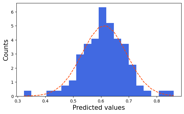
Figure 3: Distribution of predicted values for a random sample from WMT20 dataset, En-Ta language pair.

Appendix C Hyperparameter Tuning

The number of dropout runs was tuned on the $[25,200]$ interval with a step of 25 on the En-De WMT20 data. We show the results in Table 9. In preliminary experiments, we found that increasing the dropout probability beyond $0.1$ did not bring any gains, therefore we used this number. We also found that dropping only the feed-forward layers of Comet and/or the pooling layers was ineffective, therefore we applied dropout on all Comet layers for all experiments presented in this paper.

# runs	PPS $\uparrow$	UPS $\uparrow$	NLL $\downarrow$	ECE $\downarrow$	Sharp. $\downarrow$
25	0.580	0.200	1.346	0.015	0.657
50	0.581	0.204	1.334	0.015	0.635
75	0.581	0.204	1.328	0.014	0.627
100	0.582	0.206	1.323	0.014	0.624
125	0.582	0.207	1.326	0.014	0.636
150	0.582	0.209	1.323	0.014	0.631
175	0.582	0.209	1.324	0.014	0.633
200	0.582	0.210	1.322	0.015	0.623

Table 9: [DA] Segment-level results obtained with different number of dropout runs.

Appendix D Deep Ensembles

Hyperparameter	HTER	DA
Encoder Model	XLM-R (base)	XLM-R (large)
Optimizer	Adam	Adam
nº frozen epochs	1	0.4
Learning rate	3e-05	3e-04
Encoder Learning Rate	1e-05	1e-05
Layerwise Decay	0.95	0.95
Batch size	16	16
Loss function	Mean squared error	Mean squared error
Dropout	0.1	0.1
Hidden sizes	[3072, 1536]	[3072, 1536]
Encoder Embedding layer	Frozen	Frozen
FP precision	32	32
Nº Epochs	2	2

Table 10: Hyperparameters used to train the deep ensembles.

Table 10 shows the hyperparameters used to train the DA and HTER estimators for our deep ensembles. In both cases we trained 4 models with different seeds and used as fifth model the wmt-large-da-estimator-1719 and the wmt-large-hter-estimator available in https://github.com/Unbabel/COMET. Each of these models has 583M parameters and were trained on a single Nvidia Quadro RTX 8000 GPU for $\approx 34$ and $\approx 3.5$ hours for the DA models and HTER models, respectively. Regarding the validation performance recorded during training, the DA models achieve a PPS of $0.612\pm 0.002$, while the HTER models achieve a PPS of $0.663\pm 0.012$.

Appendix E Non-parametric Estimation of Confidence Intervals

The parametric Gaussian approach we chose to obtain confidence intervals, described in §3, fits relatively well our data (see Figure 3). However, this approach makes a strong assumption about the shape of $\hat{p}_{Q}(q)$, and therefore we experimented also with a non-parametric bootstrapping technique to estimate confidence intervals. Such approach has been successful in several NLP tasks (Koehn, 2004; Li et al., 2017; Ye et al., 2021). In this case, we construct the confidence intervals $I(\gamma)$ by using the percentile method Efron (1979); Johnson (2001). We take the range of point estimates in $\mathcal{Q}$ that cover equal $\frac{\gamma}{2}$ proportions around the median of the $\hat{p}_{Q}(q)$ distribution as the desired confidence interval, represented by the corresponding sample quantiles. Since this approach typically require many samples to obtain accurate estimates of the quantiles, we left out the deep ensemble method from this experiment (which would require training too many models) and focused only on samples obtained from MC dropout, using $M=100$ as in the parametric Gaussian experiments.

Since this approach does not produce a full distribution $\hat{p}_{Q}(q)$ but only the median $\hat{\mu}_{\mathrm{med}}$ and confidence intervals $I(\gamma)$, the evaluation metrics UPS, NLL, and sharpness cannot be directly applied. Therefore, we evaluated with the following modifications of predictive Pearson score and ECE.

Predictive Pearson score

For Pearson-related evaluation we use the PPS performance indicator defined in § 4, but we measure the correlation between groundtruth quality scores $q^{*}$ and the median $\hat{\mu}_{\mathrm{med}}$, instead of the average $\hat{\mu}$.

Calibration Error

To compute ECE we use the same method as defined in Eq. 2. We use this metric with $M=20$ to assess the ability of the non-parametric method to estimate confidence intervals.

Experiments

The results are shown in Table 11. Overall, MC dropout outperforms the baseline across both measures (except for PPS in En-Cs) but the improvement is marginal. The performance of the parametric approach for the same dataset in Table 2 is better than non-parametric for both reported ECE and PPS. Still, ECE values are close to the ones obtained with the parametric approach for all language pairs, and we can obtain a well-calibrated model with the non-parametric approach too (compared to the baseline).

The observed performance of a non-parametric approach could be limited by the number of observed samples and the method used to generate those (MC dropout). In Ye et al. (2021) a similar experiment of confidence intervals calibration was performed over $1000$ bootstrapped samples. Running this number of MC dropout runs would be very expensive in practice and out of scope of this work.

		PPS $\uparrow$	ECE $\downarrow$
En-De	MC dropout	0.576	0.016
	Baseline	0.576	0.071
En-Zh	MC dropout	0.332	0.030
	Baseline	0.329	0.062
En-Ta	MC dropout	0.657	0.024
	Baseline	0.655	0.050
Zh-En	MC dropout	0.314	0.016
	Baseline	0.313	0.057
En-Ja	MC dropout	0.640	0.015
	Baseline	0.636	0.051
En-Cs	MC dropout	0.691	0.013
	Baseline	0.695	0.053
En-Ru	MC dropout	0.536	0.019
	Baseline	0.532	0.061
En-Pl	MC dropout	0.611	0.016
	Baseline	0.608	0.052
En-Iu	MC dropout	0.300	0.016
	Baseline	0.292	0.057

Table 11: Results for segment-level DA prediction for a non-parametric approach. Underlined numbers indicate the best result for each language pair and evaluation metric. Reported are the predictive Pearson score $r(\hat{\mu}_{\mathrm{med}},q^{*})$ (PPS), where $\hat{\mu}_{\mathrm{med}}$ is the median, and the expected calibration error (ECE).

Appendix F Detection of Critical Translation Mistakes

We provide more detailed experiments of the critical translation error detection in Figure 4, showing the Recall@N and Precision@N for different error proportions from the dataset, ranging from $1\%$ to $20\%$. We can see that while increasing the proportion of errors considered critical, the Recall@N performance gap for UA-Comet and Comet decreases.

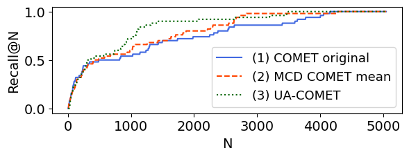
(a) Recall@N, worst 1%

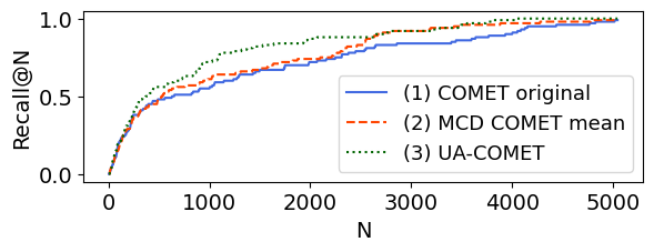
(b) Recall@N, worst 2%

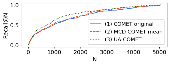
(c) Recall@N, worst 5%

(d) Recall@N, worst 10%

(e) Recall@N, worst 15%

(f) Recall@N, worst 20%

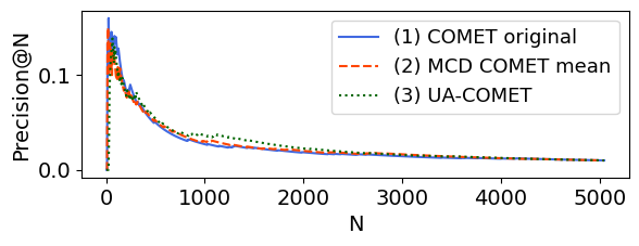
(g) Precision@N, worst 1%

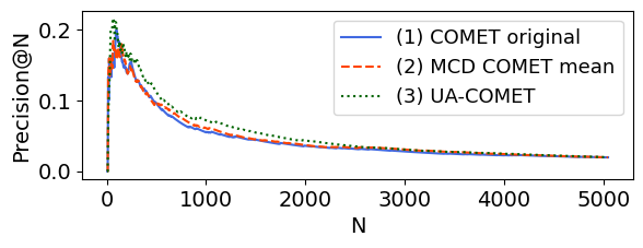
(h) Precision@N, worst 2%

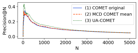
(i) Precision@N, worst 5%

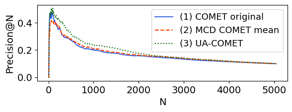
(j) Precision@N, worst 10%

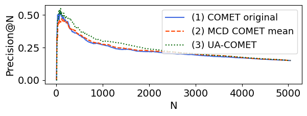
(k) Precision@N, worst 15%

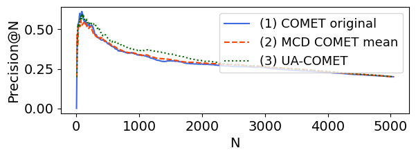
(l) Precision@N, worst 20%

Figure 4: Performance on predicting the worst MTs, using Prism pseudo-references. The continuous (blue) line corresponds to the original Comet prediction, while the dashed (orange) line to the averaged predictions obtained by MCD. The dotted (green) line corresponds to predictions using the cdf UA-Comet.

We show examples of the worst translations according to MQM scores with and without length normalisation in Tables 12 and 13 respectively, in order to better demonstrate the impact of length normalisation on the selection of critical errors.

source sentences	MT sentences	MQM
Vulnerable Dems air impeachment concerns to Pelosi	Anfällige Dems Luft Amtsenthebungsbedenken an Pelosi	17.67
Vulnerable Dems air impeachment concerns to Pelosi	Anfällige Dems Luft-Impeachment Bedenken gegen Pelosi	17.33
Vulnerable Dems air impeachment concerns to Pelosi	Verletzliche Dems-Luft-Impeachment-Bedenken gegen Pelosi	17.67
Government Retires 15 More Senior Tax Officials On Graft Charges	Regierung scheidet aus 15 weiteren hohen Steuerbeamten wegen Graft-Gebühren aus	17
Hideous’ Central Coast camouflage child rapist ordered to look at victim in court	"Hideous" Central Coast Tarnung Kindervergewaltiger bestellt, um Opfer vor Gericht zu betrachten	20.07
A third wrote: "Don’t fall for it Khloe."	Ein dritter schrieb: „Fallen Sie nicht für Khloe.“	10.37
Parents of 5-month-old stuffed in suitcase and tossed in dumpster get 6 years in prison	Eltern von 5 Monaten in Koffer gestopft und in Müllcontainer geworfen bekommen 6 Jahre Gefängnis	18.67
The Who STOP concert last night: Friday and Sunday shows CANCELLED	Das Who STOP Konzert gestern Abend: Freitag und Sonntag zeigt CANCELLED	13.67
Parents of 5-month-old stuffed in suitcase and tossed in dumpster get 6 years in prison	Eltern von 5-Monats-Alt in Koffer gefüllt und in Mülleimer geworfen bekommen 6 Jahre im Gefängnis	18.67
Vulnerable Dems air impeachment concerns to Pelosi	Vulnerable Dems Air Impeachment Bedenken für Pelosi	9.67
Brother Jailed For Life For Pakistan Social Media Star Qandeel Baloch’s Honour Killing	Bruder für Leben für Pakistan Social Media Star Qandeel Baloch s Ehre Tötung inhaftiert	15.37
Vulnerable Dems air impeachment concerns to Pelosi	Vulnerable Dems Air Impeachment Bedenken gegen Pelosi	9.33
"I can’t help the way I’m made," Whitehurst told the Sun.	„Ich kann nicht anders, wie ich gemacht bin“, sagte Whitehurst der Sonne.	12.67
"I can’t help the way I’m made," Whitehurst told the Sun.	"Ich kann nicht anders, als ich gemacht bin", sagte Whitehurst der Sonne.	12.4
Parents of 5-month-old stuffed in suitcase and tossed in dumpster get 6 years in prison	Eltern von 5 Monaten, die in Koffer gestopft und in Müllcontainer geworfen werden, bekommen 6 Jahre Gefängnis	18.33
Woman STRIPS TO NOTHING in Walmart to prove she didn’t steal	Frau STRIPS TO NOTHING in Walmart zu beweisen, dass sie nicht stehlen	11.33
Brother Jailed For Life For Pakistan Social Media Star Qandeel Baloch’s Honour Killing	Bruder lebenslang für Pakistan eingesperrt Social Media Star Qandeel Balochs Ehrenmord	14.03
Sacramento police also announced Thursday their internal investigation did not find any policy or training violations.	Sacramento Polizei kündigte auch am Donnerstag ihre internen Ermittlungen fand keine Richtlinien oder Trainingsverstöße.	18
Man pleads guilty in kidnap, torture plot of plastic surgeon	Mann bekennt sich schuldig bei Entführung, Folter des plastischen Chirurgen	11

Table 12: Worst 20 translations according to MQM scores (averaged over 3 annotators) for En-De, normalised by sentence length (word number). Highlighted rows are common in both ranking approaches.

source sentences	MT sentences	MQM
"[Barr has] gone rogue," Pelosi told MSNBC Friday. "I think where they’re going is a cover-up of a cover-up. I think it’s sad, to have a Justice Department go so rogue. Well, they have been for a while. And now it just makes matters worse."	„[Barr hat] gegangen Schurken“, Pelosi sagte MSNBC Freitag. „Ich denke, wohin sie gehen, ist eine Vertuschung einer Vertuschung. Ich denke, es ist traurig, ein Justizministerium gehen so Schurken. Nun, sie haben für eine Weile. Und jetzt macht es die Sache nur noch schlimmer“.	22.33
Add Lancaster of Pikeville told North Carolina Education Lottery officials he used five sets of his own numbers to buy a Cash 5 ticket with five plays for Monday night’s drawing when he stopped at Wissam & Brothers Inc. in Pikeville.	Fügen Sie Lancaster von Pikeville sagte North Carolina Education Lottery Beamten er fünf Sätze seiner eigenen Zahlen verwendet, um ein Cash 5 Ticket mit fünf Spielen für Montag Abend Zeichnung zu kaufen, als er bei Wissam & Brothers Inc. in Pikeville hielt.	22.33
Hideous’ Central Coast camouflage child rapist ordered to look at victim in court	"Hideous" Central Coast Tarnung Kindervergewaltiger bestellt, um Opfer vor Gericht zu betrachten	20.06
Trump is singing from a similar songbook. His administration’s Muslim-majority travel ban echoes the Islamophobia that often informs Modi’s policymaking. Its callousness toward refugees mirrors the Indian government’s disdain for the Rohingya population’s suffering, and its detention camps parallel the ones the Modi regime is setting up. Trump’s stirring of racial animosity is analogous to troublesome rhetoric from a number of Modi’s cabinet members.	Trump singt aus einem ähnlichen Liederbuch. Das Reiseverbot seiner Regierung mit muslimischer Mehrheit spiegelt die Islamophobie wider, die oft Modis Politik informiert. Seine Anrufung gegenüber Flüchtlingen spiegelt die Verachtung der indischen Regierung für das Leiden der Rohingya-Bevölkerung und ihre Gefangenenlager parallel zu denen wider, die das Modi-Regime einrichtet. Trumps Aufregung rassischer Feindseligkeit ist analog zur lästigen Rhetorik einer Reihe von Modis Kabinettsmitgliedern.	19.67
"Currently we are targeting young people 18 to 24 years. For the young people that’s the age bracket we are looking at but of course any one above 18 and it’s because we do not have evidence of children by the Constitution but as more evidence unfolds we are going to get there. For the men, we give the kit to the mother and they take it to the partner, key and priority populations such sex workers," Mr Geoffrey Tasi, the technical officer-in-charge of HIV testing services, said yesterday.	"Derzeit richten wir uns an Jugendliche im Alter von 18 bis 24 Jahren. Für die jungen Leute, die die Altersgruppe sind, die wir betrachten, aber natürlich jede über 18 und es ist, weil wir keine Beweise für Kinder durch die Verfassung haben, aber als mehr Beweise sich entfalten, werden wir dorthin gelangen. Für die Männer geben wir das Kit an die Mutter und sie bringen es dem Partner, Schlüssel- und Priorat solcher Sexarbeiterinnen", sagte Geoffrey Tasi, der für HIV-Testdienste zuständige technische Beamte, gestern.	19.07
Parents of 5-month-old stuffed in suitcase and tossed in dumpster get 6 years in prison	Eltern von 5-Monats-Alt in Koffer gefüllt und in Mülleimer geworfen bekommen 6 Jahre im Gefängnis	18.67
Parents of 5-month-old stuffed in suitcase and tossed in dumpster get 6 years in prison	Eltern von 5 Monaten in Koffer gestopft und in Müllcontainer geworfen bekommen 6 Jahre Gefängnis	18.67
Parents of 5-month-old stuffed in suitcase and tossed in dumpster get 6 years in prison	Eltern von 5 Monaten, die in Koffer gestopft und in Müllcontainer geworfen werden, bekommen 6 Jahre Gefängnis	18.33
Sacramento police also announced Thursday their internal investigation did not find any policy or training violations.	Sacramento Polizei kündigte auch am Donnerstag ihre internen Ermittlungen fand keine Richtlinien oder Trainingsverstöße.	18
Vulnerable Dems air impeachment concerns to Pelosi	Verletzliche Dems-Luft-Impeachment-Bedenken gegen Pelosi	17.67
The 35-year-old star dumped the NBA player for good earlier this year after he was accused of cheating on her with family friend Jordyn Woods - having previously cheated when she was nine months pregnant with their daughter, True.	Der 35-jährige Star warf die NBA-Spielerin Anfang des Jahres endgültig ab, nachdem er beschuldigt wurde, sie mit Familienfreund Jordyn Woods betrogen zu haben - nachdem sie zuvor betrogen hatte, als sie im neunten Monat mit ihrer Tochter True schwanger war.	17.67
Vulnerable Dems air impeachment concerns to Pelosi	Anfällige Dems Luft Amtsenthebungsbedenken an Pelosi	17.67
It comes just days after Tristan wrote: "Perfection" alongside the heart eye emojis underneath one of the reality stars other photos, which saw her modelling for Guess Jeans.	Es kommt nur wenige Tage, nachdem Tristan geschrieben hat: "Perfection" neben den Herzaugen-Emojis unter einem der Reality-Stars andere Fotos, die sie für Guess Jeans modellieren sah.	17.43
"You’re going out a youngster, but you’ve got to come back a star!" Blanks wrote in an Instagram caption on Wednesday, quoting the film "42nd Street."	"Du gehst als Jugendlicher aus, aber du musst einen Stern zurückkommen!" Blanks schrieb am Mittwoch in einem Instagram-Titel den Film "42nd Street".	17.43
"Sounding more and more like the so-called whistle-blower isn’t a whistle-blower at all," he tweeted. "In addition, all second-hand information that proved to be so inaccurate that there may not have been somebody else, a leaker or spy, feeding it to him or her? A partisan operative?"	"Immer mehr nach dem sogenannten Whistleblower zu klingen, ist überhaupt kein Whistleblower", twitterte er. "Außerdem alle Informationen aus zweiter Hand, die sich als so ungenau erwiesen haben, dass möglicherweise nicht jemand anderes, ein Leckerbissen oder ein Spion, sie ihm oder ihr gefüttert hat? Ein Partisanen-Agent?"	17.43
"Currently, 86 per cent people living with HIV know their status; that means it leave us with 14 per cent of those living with HIV and do not know their status. So how do we now utilise that additional innovation. Really for me this is it … how do we now move from this kit and create demand, especially for that 14 per cent that are sick and they need care and they are not getting care," Dr Atwine said.	"Derzeit kennen 86 Prozent der HIV-Infizierten ihren Status; Das bedeutet, dass wir bei 14 Prozent der HIV-Infizierten leben und ihren Status nicht kennen. Wie können wir nun diese zusätzliche Innovation nutzen? Wirklich für mich ist es … Wie können wir jetzt von diesem Kit wegkommen und Nachfrage schaffen, vor allem für die 14 Prozent, die krank sind und Pflege brauchen und sie nicht versorgt werden", sagte Dr. Atwine.	17.4
Sacramento police also announced Thursday their internal investigation did not find any policy or training violations.	Sacramento Polizei kündigte auch am Donnerstag ihre interne Untersuchung keine Politik oder Ausbildung Verstöße gefunden.	17.33
"Currently we are targeting young people 18 to 24 years. For the young people that’s the age bracket we are looking at but of course any one above 18 and it’s because we do not have evidence of children by the Constitution but as more evidence unfolds we are going to get there. For the men, we give the kit to the mother and they take it to the partner, key and priority populations such sex workers," Mr Geoffrey Tasi, the technical officer-in-charge of HIV testing services, said yesterday.	„Gegenwärtig richten wir uns an junge Menschen zwischen 18 und 24 Jahren. Für die jungen Menschen ist das die Altersgruppe, die wir betrachten, aber natürlich jede über 18, und das liegt daran, dass wir keine Beweise für Kinder durch die Verfassung haben, aber wenn sich mehr Beweise entwickeln, werden wir dorthin gelangen. Für die Männer geben wir das Kit an die Mutter und sie bringen es an den Partner, Schlüssel- und Prioritätspopulationen wie Sexarbeiter“, sagte gestern Geoffrey Tasi, der zuständige technische Offizier für HIV-Tests.	17.33
Vulnerable Dems air impeachment concerns to Pelosi	Anfällige Dems Luft-Impeachment Bedenken gegen Pelosi	17.33

Table 13: Worst 20 translations according to MQM scores (averaged over 3 annotators) for En-De. Highlighted rows are common in both ranking approaches.

References

- Ashukha et al. (2020) Arsenii Ashukha, Alexander Lyzhov, Dmitry Molchanov, and Dmitry Vetrov. 2020. Pitfalls of in-domain uncertainty estimation and ensembling in deep learning. In International Conference on Learning Representations.
- Beck et al. (2016) Daniel Beck, Lucia Specia, and Trevor Cohn. 2016. Exploring prediction uncertainty in machine translation quality estimation. In Proceedings of The 20th SIGNLL Conference on Computational Natural Language Learning, pages 208–218, Berlin, Germany. Association for Computational Linguistics.
- Blatz et al. (2004) John Blatz, Erin Fitzgerald, George Foster, Simona Gandrabur, Cyril Goutte, Alex Kulesza, Alberto Sanchis, and Nicola Ueffing. 2004. Confidence estimation for machine translation. In COLING 2004: Proceedings of the 20th International Conference on Computational Linguistics, pages 315–321, Geneva, Switzerland. COLING.
- Burchardt and Lommel (2014) Aljoscha Burchardt and Arle Lommel. 2014. Practical Guidelines for the Use of MQM in Scientific Research on Translation quality. (access date: 2020-05-26).
- Charpentier et al. (2020) Bertrand Charpentier, Daniel Zügner, and Stephan Günnemann. 2020. Posterior network: Uncertainty estimation without ood samples via density-based pseudo-counts. Advances in Neural Information Processing Systems, 33:1356–1367.
- Denkowski and Lavie (2014) Michael Denkowski and Alon Lavie. 2014. Meteor universal: Language specific translation evaluation for any target language. In Proceedings of the Ninth Workshop on Statistical Machine Translation, pages 376–380, Baltimore, Maryland, USA. Association for Computational Linguistics.
- Desai and Durrett (2020) Shrey Desai and Greg Durrett. 2020. Calibration of pre-trained transformers. In Proceedings of the 2020 Conference on Empirical Methods in Natural Language Processing (EMNLP), pages 295–302, Online. Association for Computational Linguistics.
- Dietterich (2000) Thomas G. Dietterich. 2000. Ensemble methods in machine learning. In Proceedings of the First International Workshop on Multiple Classifier Systems, MCS ’00, page 1–15, Berlin, Heidelberg. Springer-Verlag.
- Duma and Menzel (2018) Melania Duma and Wolfgang Menzel. 2018. The benefit of pseudo-reference translations in quality estimation of MT output. In Proceedings of the Third Conference on Machine Translation: Shared Task Papers, pages 776–781, Belgium, Brussels. Association for Computational Linguistics.
- Efron (1979) B. Efron. 1979. Bootstrap methods: Another look at the jackknife. The Annals of Statistics, 7(1):1–26.
- Fomicheva et al. (2020) Marina Fomicheva, Shuo Sun, Lisa Yankovskaya, Frédéric Blain, Francisco Guzmán, Mark Fishel, Nikolaos Aletras, Vishrav Chaudhary, and Lucia Specia. 2020. Unsupervised quality estimation for neural machine translation. Transactions of the Association for Computational Linguistics, 8:539–555.
- Freitag et al. (2021) Markus Freitag, George Foster, David Grangier, Viresh Ratnakar, Qijun Tan, and Wolfgang Macherey. 2021. Experts, errors, and context: A large-scale study of human evaluation for machine translation.
- Freitag et al. (2020) Markus Freitag, David Grangier, and Isaac Caswell. 2020. BLEU might be guilty but references are not innocent. In Proceedings of the 2020 Conference on Empirical Methods in Natural Language Processing (EMNLP), pages 61–71, Online. Association for Computational Linguistics.
- Gal and Ghahramani (2016) Yarin Gal and Zoubin Ghahramani. 2016. Dropout as a bayesian approximation: Representing model uncertainty in deep learning. In Proceedings of The 33rd International Conference on Machine Learning, volume 48 of Proceedings of Machine Learning Research, pages 1050–1059, New York, New York, USA. PMLR.
- Garmash and Monz (2016) Ekaterina Garmash and Christof Monz. 2016. Ensemble learning for multi-source neural machine translation. In Proceedings of COLING 2016, the 26th International Conference on Computational Linguistics: Technical Papers, pages 1409–1418, Osaka, Japan. The COLING 2016 Organizing Committee.
- Graham et al. (2013) Yvette Graham, Timothy Baldwin, Alistair Moffat, and Justin Zobel. 2013. Continuous measurement scales in human evaluation of machine translation. In Proceedings of the 7th Linguistic Annotation Workshop and Interoperability with Discourse, pages 33–41, Sofia, Bulgaria. Association for Computational Linguistics.
- Graves (2011) Alex Graves. 2011. Practical variational inference for neural networks. In Advances in Neural Information Processing Systems, volume 24. Curran Associates, Inc.
- Guo et al. (2017) Chuan Guo, Geoff Pleiss, Yu Sun, and Kilian Q. Weinberger. 2017. On calibration of modern neural networks. In Proceedings of the 34th International Conference on Machine Learning, volume 70 of Proceedings of Machine Learning Research, pages 1321–1330. PMLR.
- Hora (1996) Stephen C. Hora. 1996. Aleatory and epistemic uncertainty in probability elicitation with an example from hazardous waste management. Reliability Engineering & System Safety, 54(2):217–223. Treatment of Aleatory and Epistemic Uncertainty.
- Huellermeier and Waegeman (2021) Eyke Huellermeier and Willem Waegeman. 2021. Aleatoric and epistemic uncertainty in machine learning : an introduction to concepts and methods. Machine Learning, 110(3):457–506.
- Jain et al. (2020) Siddhartha Jain, Ge Liu, Jonas Mueller, and David Gifford. 2020. Maximizing overall diversity for improved uncertainty estimates in deep ensembles. Proceedings of the AAAI Conference on Artificial Intelligence, 34(04):4264–4271.
- Jiang et al. (2011) Xiaoqian Jiang, Melanie Osl, Jihoon Kim, and Lucila Ohno-Machado. 2011. Calibrating predictive model estimates to support personalized medicine. Journal of the American Medical Informatics Association, 19(2):263–274.
- Johnson (2001) Roger W. Johnson. 2001. An introduction to the bootstrap. Teaching Statistics, 23(2):49–54.
- Kendall et al. (2017) Alex Kendall, Vijay Badrinarayanan, and Roberto Cipolla. 2017. Bayesian segnet: Model uncertainty in deep convolutional encoder-decoder architectures for scene understanding. In Proceedings of the British Machine Vision Conference (BMVC), pages 57.1–57.12. BMVA Press.
- Kendall and Gal (2017) Alex Kendall and Yarin Gal. 2017. What uncertainties do we need in bayesian deep learning for computer vision? In Advances in Neural Information Processing Systems, volume 30. Curran Associates, Inc.
- Kepler et al. (2019) Fabio Kepler, Jonay Trénous, Marcos Treviso, Miguel Vera, and André F. T. Martins. 2019. OpenKiwi: An open source framework for quality estimation. In Proceedings of the 57th Annual Meeting of the Association for Computational Linguistics: System Demonstrations, pages 117–122, Florence, Italy. Association for Computational Linguistics.
- Kiureghian and Ditlevsen (2009) Armen Der Kiureghian and Ove Ditlevsen. 2009. Aleatory or epistemic? does it matter? Structural Safety, 31(2):105–112. Risk Acceptance and Risk Communication.
- Koehn (2004) Philipp Koehn. 2004. Statistical significance tests for machine translation evaluation. In Proceedings of the 2004 Conference on Empirical Methods in Natural Language Processing, pages 388–395, Barcelona, Spain. Association for Computational Linguistics.
- Kuleshov et al. (2018a) Volodymyr Kuleshov, Nathan Fenner, and Stefano Ermon. 2018a. Accurate uncertainties for deep learning using calibrated regression. In Proceedings of the 35th International Conference on Machine Learning, volume 80 of Proceedings of Machine Learning Research, pages 2796–2804. PMLR.
- Kuleshov et al. (2018b) Volodymyr Kuleshov, Nathan Fenner, and Stefano Ermon. 2018b. Accurate uncertainties for deep learning using calibrated regression. In Proceedings of the 35th International Conference on Machine Learning, volume 80 of Proceedings of Machine Learning Research, pages 2796–2804. PMLR.
- Lakshminarayanan et al. (2017) Balaji Lakshminarayanan, Alexander Pritzel, and Charles Blundell. 2017. Simple and scalable predictive uncertainty estimation using deep ensembles. In Advances in Neural Information Processing Systems, volume 30. Curran Associates, Inc.
- Li et al. (2017) Junhui Li, Deyi Xiong, Zhaopeng Tu, Muhua Zhu, Min Zhang, and Guodong Zhou. 2017. Modeling source syntax for neural machine translation. arXiv preprint arXiv:1705.01020.
- Lommel et al. (2014) Arle Lommel, Aljoscha Burchardt, and Hans Uszkoreit. 2014. Multidimensional quality metrics (MQM): A framework for declaring and describing translation quality metrics. Tradumàtica: tecnologies de la traducció, 0:455–463.
- Mackay (1992) David John Cameron Mackay. 1992. Bayesian Methods for Adaptive Models. Ph.D. thesis, California Institute of Technology, USA. UMI Order No. GAX92-32200.
- Malinin and Gales (2018) Andrey Malinin and Mark Gales. 2018. Predictive uncertainty estimation via prior networks. In Proceedings of the 32nd International Conference on Neural Information Processing Systems, pages 7047–7058.
- Malinin and Gales (2021) Andrey Malinin and Mark Gales. 2021. Uncertainty estimation in autoregressive structured prediction. In International Conference on Learning Representations.
- Mathur et al. (2020) Nitika Mathur, Johnny Wei, Markus Freitag, Qingsong Ma, and Ondřej Bojar. 2020. Results of the WMT20 metrics shared task. In Proceedings of the Fifth Conference on Machine Translation, pages 688–725, Online. Association for Computational Linguistics.
- McClure and Kriegeskorte (2017) Patrick McClure and Nikolaus Kriegeskorte. 2017. Robustly representing uncertainty in deep neural networks through sampling. Second Workshop on Bayesian Deep Learning (NIPS 2017).
- Naeini et al. (2015) Mahdi Pakdaman Naeini, Gregory F. Cooper, and Milos Hauskrecht. 2015. Obtaining well calibrated probabilities using bayesian binning. In Proceedings of the Twenty-Ninth AAAI Conference on Artificial Intelligence, AAAI’15, page 2901–2907. AAAI Press.
- Niculescu-Mizil and Caruana (2005) Alexandru Niculescu-Mizil and Rich Caruana. 2005. Predicting good probabilities with supervised learning. In Proceedings of the 22nd International Conference on Machine Learning, ICML ’05, page 625–632, New York, NY, USA. Association for Computing Machinery.
- Ott et al. (2018) Myle Ott, Michael Auli, David Grangier, and Marc’Aurelio Ranzato. 2018. Analyzing uncertainty in neural machine translation. In Proceedings of the 35th International Conference on Machine Learning, volume 80 of Proceedings of Machine Learning Research, pages 3956–3965. PMLR.
- Papineni et al. (2002) Kishore Papineni, Salim Roukos, Todd Ward, and Wei-Jing Zhu. 2002. Bleu: a method for automatic evaluation of machine translation. In Proceedings of the 40th Annual Meeting of the Association for Computational Linguistics, pages 311–318, Philadelphia, Pennsylvania, USA. Association for Computational Linguistics.
- Pearce et al. (2020) Tim Pearce, Felix Leibfried, and Alexandra Brintrup. 2020. Uncertainty in neural networks: Approximately bayesian ensembling. In Proceedings of the Twenty Third International Conference on Artificial Intelligence and Statistics, volume 108 of Proceedings of Machine Learning Research, pages 234–244. PMLR.
- Platt (1999) John C. Platt. 1999. Probabilistic outputs for support vector machines and comparisons to regularized likelihood methods. In Advances in Large Margin Classifiers, pages 61–74. MIT Press.
- Popović (2015) Maja Popović. 2015. chrF: character n-gram F-score for automatic MT evaluation. In Proceedings of the Tenth Workshop on Statistical Machine Translation, pages 392–395, Lisbon, Portugal. Association for Computational Linguistics.
- Quirk (2004) Christopher B. Quirk. 2004. Training a sentence-level machine translation confidence measure. In Proceedings of the Fourth International Conference on Language Resources and Evaluation (LREC’04), Lisbon, Portugal. European Language Resources Association (ELRA).
- Raftery et al. (2005) Adrian E. Raftery, Tilmann Gneiting, Fadoua Balabdaoui, and Michael Polakowski. 2005. Using bayesian model averaging to calibrate forecast ensembles. Monthly Weather Review, 133(5):1155 – 1174.
- Ranasinghe et al. (2020) Tharindu Ranasinghe, Constantin Orasan, and Ruslan Mitkov. 2020. TransQuest at WMT2020: Sentence-level direct assessment. In Proceedings of the Fifth Conference on Machine Translation, pages 1049–1055, Online. Association for Computational Linguistics.
- Rei et al. (2020a) Ricardo Rei, Craig Stewart, Ana C Farinha, and Alon Lavie. 2020a. COMET: A neural framework for MT evaluation. In Proceedings of the 2020 Conference on Empirical Methods in Natural Language Processing (EMNLP), pages 2685–2702, Online. Association for Computational Linguistics.
- Rei et al. (2020b) Ricardo Rei, Craig Stewart, Ana C Farinha, and Alon Lavie. 2020b. Unbabel’s participation in the WMT20 metrics shared task. In Proceedings of the Fifth Conference on Machine Translation, pages 911–920, Online. Association for Computational Linguistics.
- Scarton and Specia (2014) Carolina Scarton and Lucia Specia. 2014. Document-level translation quality estimation: exploring discourse and pseudo-references. In Proceedings of the 17th Annual conference of the European Association for Machine Translation, pages 101–108, Dubrovnik, Croatia. European Association for Machine Translation.
- Sellam et al. (2020) Thibault Sellam, Dipanjan Das, and Ankur Parikh. 2020. BLEURT: Learning robust metrics for text generation. In Proceedings of the 58th Annual Meeting of the Association for Computational Linguistics, pages 7881–7892, Online. Association for Computational Linguistics.
- Sensoy et al. (2018) Murat Sensoy, Lance Kaplan, and Melih Kandemir. 2018. Evidential deep learning to quantify classification uncertainty. In Proceedings of the 32nd International Conference on Neural Information Processing Systems, pages 3183–3193.
- Smith and Gal (2018) Lewis Smith and Yarin Gal. 2018. Understanding measures of uncertainty for adversarial example detection. arXiv preprint arXiv:1803.08533.
- Snover et al. (2006) Matthew Snover, Bonnie Dorr, Rich Schwartz, Linnea Micciulla, and John Makhoul. 2006. A study of translation edit rate with targeted human annotation. In Proceedings of the 7th Conference of the Association for Machine Translation in the Americas: Technical Papers, pages 223–231, Cambridge, Massachusetts, USA. Association for Machine Translation in the Americas.
- Specia et al. (2017) Lucia Specia, Kim Harris, Aljoscha Burchardt, Marco Turchi, Matteo Negri, and Inguna Skadina. 2017. Translation quality and productivity: A study on rich morphology languages. In Machine Translation Summit XVI, pages 55–71.
- Specia et al. (2018) Lucia Specia, Carolina Scarton, and Gustavo Henrique Paetzold. 2018. Quality estimation for machine translation. Synthesis Lectures on Human Language Technologies, 11(1):1–162.
- Srivastava et al. (2014) Nitish Srivastava, Geoffrey Hinton, Alex Krizhevsky, Ilya Sutskever, and Ruslan Salakhutdinov. 2014. Dropout: A simple way to prevent neural networks from overfitting. Journal of Machine Learning Research, 15(56):1929–1958.
- Sun et al. (2020) Shuo Sun, Francisco Guzmán, and Lucia Specia. 2020. Are we estimating or guesstimating translation quality? In Proceedings of the 58th Annual Meeting of the Association for Computational Linguistics, pages 6262–6267, Online. Association for Computational Linguistics.
- Thompson and Post (2020a) Brian Thompson and Matt Post. 2020a. Automatic machine translation evaluation in many languages via zero-shot paraphrasing. In Proceedings of the 2020 Conference on Empirical Methods in Natural Language Processing (EMNLP), pages 90–121, Online. Association for Computational Linguistics.
- Thompson and Post (2020b) Brian Thompson and Matt Post. 2020b. Paraphrase generation as zero-shot multilingual translation: Disentangling semantic similarity from lexical and syntactic diversity. In Proceedings of the Fifth Conference on Machine Translation, pages 561–570, Online. Association for Computational Linguistics.
- Toral (2020) Antonio Toral. 2020. Reassessing claims of human parity and super-human performance in machine translation at WMT 2019. In Proceedings of the 22nd Annual Conference of the European Association for Machine Translation, pages 185–194, Lisboa, Portugal. European Association for Machine Translation.
- Tran et al. (2019) Dustin Tran, Mike Dusenberry, Mark van der Wilk, and Danijar Hafner. 2019. Bayesian layers: A module for neural network uncertainty. In Advances in Neural Information Processing Systems, volume 32. Curran Associates, Inc.
- Verdoja and Kyrki (2020) Francesco Verdoja and Ville Kyrki. 2020. Notes on the behavior of mc dropout. arXiv preprint arXiv:2008.02627.
- Wang et al. (2019) Shuo Wang, Yang Liu, Chao Wang, Huanbo Luan, and Maosong Sun. 2019. Improving back-translation with uncertainty-based confidence estimation. In Proceedings of the 2019 Conference on Empirical Methods in Natural Language Processing and the 9th International Joint Conference on Natural Language Processing (EMNLP-IJCNLP), pages 791–802, Hong Kong, China. Association for Computational Linguistics.
- Welling and Teh (2011) Max Welling and Yee Whye Teh. 2011. Bayesian learning via stochastic gradient langevin dynamics. In Proceedings of the 28th International Conference on International Conference on Machine Learning, ICML’11, page 681–688, Madison, WI, USA. Omnipress.
- Xia et al. (2020) Mengzhou Xia, Antonios Anastasopoulos, Ruochen Xu, Yiming Yang, and Graham Neubig. 2020. Predicting performance for natural language processing tasks. In Proceedings of the 58th Annual Meeting of the Association for Computational Linguistics, pages 8625–8646, Online. Association for Computational Linguistics.
- Ye et al. (2021) Zihuiwen Ye, Pengfei Liu, Jinlan Fu, and Graham Neubig. 2021. Towards more fine-grained and reliable NLP performance prediction. In Proceedings of the 16th Conference of the European Chapter of the Association for Computational Linguistics: Main Volume, pages 3703–3714, Online. Association for Computational Linguistics.
- Zhang et al. (2020) Tianyi Zhang, Varsha Kishore, Felix Wu, Kilian Q. Weinberger, and Yoav Artzi. 2020. Bertscore: Evaluating text generation with bert. In International Conference on Learning Representations.