Feedback-Based Optimization with Sub-Weibull Gradient Errors and Intermittent Updates
Ana M. Ospina
Nicola Bastianello
and Emiliano Dall’Anese
A. Ospina and E. Dall’Anese are with Department of Electrical, Computer and Energy Engineering, University of Colorado Boulder, Boulder, CO, USA, {ana.ospina, emiliano.dallanese}@colorado.edu; N. Bastianello is with the Department of Information Engineering, University of Padova, Padova, Italy, bastian4@dei.unipd.it. This work was supported in part by the NSF CAREER award 1941896.
Abstract
This paper considers a feedback-based projected gradient method for optimizing systems modeled as algebraic maps. The focus is on a setup where the gradient is corrupted by random errors that follow a sub-Weibull distribution, and where the measurements of the output – which replace the input-output map of the system in the algorithmic updates – may not be available at each iteration. The sub-Weibull error model is particularly well-suited in frameworks where the cost of the problem is learned via Gaussian Process (GP) regression (from functional evaluations) concurrently with the execution of the algorithm; however, it also naturally models setups where nonparametric methods and neural networks are utilized to estimate the cost. Using the sub-Weibull model, and with Bernoulli random variables modeling missing measurements of the system output, we show that the online algorithm generates points that are within a bounded error from the optimal solutions. In particular, we provide error bounds in expectation and in high probability. Numerical results are presented in the context of a demand response problem in smart power grids.
{IEEEkeywords}
Optimization, Optimization algorithms.
1 Introduction
\IEEEPARstart
We consider optimization problems associated with systems that feature controllable inputs and unknown exogenous inputs . Modeling the system as an algebraic map , where is well-defined [1, 2, 3], the objective is to steer the system to optimal solutions of the following time-varying problem111Notation: Upper-case (lower-case) boldface letters will be used for matrices (column vectors); denotes transposition. For a given vector , .
For a random variable , denotes the expected value of , and denotes the probability of taking values smaller than or equal to . For a continuously-differentiable function , the gradient is denoted by . Given a convex set , denotes the projection of onto . is the identity mapping. Finally, will denote the Euler’s number.
(1)
where is the time index, is a time-varying constraint set for the inputs, is a cost associated with the inputs, and is a cost associated with the outputs. We consider the case where is unknown or it cannot be directly measured; with not known, (1) can be solved using online algorithms of the following form (see, e.g.,[2, 3]):
(2)
where is the Jacobian of ( here denotes the th entry of ). The algorithm is “feedback-based” since the output measurement replaces the system model in the computation of the gradient.
We consider an online algorithm similar to (2), but in a setting where: (i) the gradient is corrupted by random errors that follow a sub-Weibull distribution [4]; and, (ii) measurements are noisy and may not be available at each time . The latter models processing and communication bottlenecks in the sensing layers of the system (for example, in power grid metering systems and transportation systems). On the other hand, the sub-Weibull model allows us to consider concurrent learning and optimization frameworks where the costs and are learned via Gaussian Process (GP) regression [5], parametric methods [6], non-parametric methods [7], and neural networks [8] from both a set of recorded data and (an infrequent set of) functional evaluations acquired during the execution of the algorithm. In this paper, we particularly highlight the use of GPs [9, 10]. Learning the cost concurrently with the execution of the algorithm finds ample applications in cyber-physical systems with human-in-the-loop [11], where models users’ preferences, as well as data-enabled and perception-based optimization [12] where is learned from data.
The ability of our framework to model various learning settings is grounded on the fact that the sub-Weibull distribution includes sub-Gaussian and sub-exponential errors as sub-cases, as well as random errors whose distribution has a finite support [4, 13].
Prior works. Prior works in the context of feedback-based optimization considered time-invariant costs [2, 14, 15] and time-varying costs [3, 16, 17]; the convergence of algorithms were investigated when the cost is known, measurements are noiseless, and measurements are received at each iteration (see also the survey [1] for a comprehensive list of references).
Online optimization methods with concurrent learning of the cost with GPs were considered in [9] for functions satisfying the Polyak-Łojasiewicz inequality; the algorithm employed the upper confidence bound and the regret was investigated. Quadratic functions were considered in [6], and they were estimated via recursive least squares. However, in [9, 6], algorithms were not implemented with a system in the loop and no missing measurements were considered.
Online algorithms with concurrent learning via shape-constrained GP were considered in [18]; however, only bounds in expectation for the regret were provided. High probability convergence results were provided in [10] for non-monotone games, where the pseudo-gradient is learned from data.
Although it is not the main focus of this paper, we also acknowledge works on zeroth-order methods (see, e.g., [19, 20]) where gradient errors emerge from single- or multi-point gradient estimation; our framework based on a sub-Weibull model can be applied to derive convergence bounds when the gradient in (2) is estimated via single- or multi-point estimation. Finally, we mention that several convergence results have been derived for classical online algorithms [21, 22], including asynchronous implementations [23]; our results provide extensions to cases with sub-Weibull gradient errors.
Contributions. The main contributions of this paper are as follows. C1) We consider an online feedback-based projected gradient descent method with intermittent updates and with noisy gradients. We provide new bounds for the error in expectation that hold iteration-wise, where is the sequence generated by the algorithm; to this end, missing measurements are modeled as Bernoulli random variables. C2) We provide new bounds on in high probability; the bounds are derived by adopting a sub-Weibull distribution for the error affecting the gradient. C3) We show how our framework models concurrent learning approaches, where one leverages functional evaluations to learn the unknown cost via GPs during the execution of the algorithm. C4) We test the performance of our algorithm in cases where the cost is estimated via GPs and feedforward neural networks.
The remainder of this paper is organized as follows. Section 2 introduces preliminary definitions. Section 3 presents the proposed algorithm and provides the corresponding analysis. Section 4 presents the concurrent learning approach. Section 5 presents numerical results on a demand response problem, while Section 6 concludes the paper.
2 Preliminaries
In this section, we introduce the class of sub-Weibull random variables and provide relevant properties. For a random variable (rv) , when the -th moment of exists for some , we define .
A random variable is sub-Weibull if such that (s.t.) one of the following conditions is satisfied:
(i)
s.t. , .
(ii)
s.t. , .
The parameters differ by a constant that depends on ; in particular, if property (ii) holds with parameter , then property (i) holds with . Hereafter, we use the short-hand notation to indicate that is a sub-Weibull rv according to Definition 1(ii) (i.e., , ). We note that the sub-Weibull class includes sub-Gaussian and sub-exponential rvs as sub-cases; in particular, if and we have sub-Gaussian and sub-exponential rvs, respectively. Furthermore, if a rv has a distribution with finite support, it belongs to the sub-Gaussian class (by Hoeffding’s inequality [13, Theorem 2.2.6]) and, thus, to the sub-Weibull class.
(Closure of sub-Weibull class [24]) Let , , based on Definition 1(ii).
(a)
Product by scalar: Let , then .
(b)
Sum by scalar: Let , then .
(c)
Sum: Let be possibly dependent; then, .
(d)
Product: Let be independent; then, .
Proposition 3
(High probability bound [4])
Let according to Definition 1(ii), for some and . Then, for any , the bound:
(3)
holds with probability .
3 Online Algorithm
In this section, we consider an online feedback-based algorithm of the form (2) to solve (1) where: (i) we utilize noisy measurements of the output , where is a measurement noise, instead of requiring full knowledge of the map and of the vector ; (ii) we rely on inexact gradient information; and, (iii) the measurements of may not be received at each iteration. Accordingly, the online algorithm is as follows (where we recall that is the time index):
(4)
where and
are approximations of the gradients and , respectively, with and random vectors that model the gradient errors. As discussed in Section 1, errors in the gradients emerge when a concurrent learning approach is utilized to estimate the functions and from samples using, e.g., GPs [9], parametric methods [6], non-parametric methods [7], or neural networks [8]. Additional sources of errors include the noise affecting the measurement of . Hereafter, we denote the overall gradient error as .
where is a rv taking values in the set , and is used to indicate whether the measurement of the system output is received or not. When a measurement is not received, we still utilize a projection onto the time-varying set . In the following, we introduce the main assumptions and we analyze the performance of the online algorithm (5).
3.1 Assumptions
Here, we outline the main assumptions used in the paper.
Assumption 1
The set is non-empty, convex and compact for all .
Assumption 2
For any , the function is convex over , . Moreover, the composite function is -strongly convex and -smooth over , for some and .
We recall that is -smooth over , for some , if it is differentiable and . The previous assumptions imply that the norm of the gradient of is bounded over the compact set . Assumption 2 also implies that there is a unique optimizer for each . Furthermore, the map is -Lipschitz with (see [25, Section 5.1]); if , then ; in other words, the map is contractive.
Assumption 3
The rv is Bernoulli distributed with parameter . The rvs are i.i.d..
Assumption 4
For all , s.t. each entry of the vector is according to Definition 1(ii). Moreover, is independent of .
Assumption 5
For all , s.t. each entry of the vector is , according to Definition 1(ii). Moreover, is independent of .
The following lemma is then presented.
Lemma 1
Suppose that Assumptions 4-5 hold. Then, is a sub-Weibull rv and, in particular, .
This lemma can be proved by using [24, Lemma 3.4] and part (c) of Proposition 2; the proof is omitted.
3.2 Convergence Analysis
Our analysis seeks bounds on the error , , where we recall that is the unique optimal solution of (1) at time . To this end, we introduce the well-known definition of path length , which measures the temporal variability of the optimal solution of (1). Finally, we let to make the notation lighter. The main result of the paper is stated in the following.
Theorem 1
Let Assumptions 1-5 hold, and let be a sequence generated by (5) for a given initial point . Recall that and .
Then, the following holds for all :
1(ii) For any , the following bound holds with probability :
(6)
where , , , and where the function is defined as .
Proof 3.2.
See the Appendix.
We note that, if , then for all ; in this case,
letting , the claim of Theorem 1(i) implies that
(7)
where the term as . From (7), it is evident that the error is asymptotically bounded in expectation, with an error bound that depends on the variability of the optimal solution, the mean of the norm of the gradient error, and the Bernoulli parameter .
We also draw a link with stability of stochastic discrete-time systems [26, 27] by noting that (7) establishes that the stochastic algorithm (5) renders the set exponentially input-to-state stable (E-ISS) in expectation.
Theorem 1(ii) asserts that is bounded in high probability. Since is monotonically decreasing, as ; thus, Theorem 1(ii) provides an asymptotic error bound that holds in high probability. We also note that the first term on the right-hand-side of (6) is a function [27]; upper-bounding the second term as , we obtain a result in terms of ISS in high-probability under a sub-Weibull error model.
4 Optimization with Concurrent GP Learning
In this section, we provide an example of a framework where the cost function is estimated using GPs during the execution of the online algorithm (5). We will show that the results of Theorem 1 directly apply to this framework.
To streamline exposition, suppose that the function is known, and the function is static but unknown (a similar approach can be used for time-varying functions). Furthermore, suppose that where is a cost associated with the -th input. We then consider a concurrent learning approach where we estimate each function via GP, based on noisy functional evaluations [9].
A GP is a stochastic process and is specified by its mean function and its covariance function [5]. Accordingly, let be characterized by a GP, i.e., for any , and . Let be the set of sampling points at times ; let , with Gaussian noise, be the noisy functional evaluation at ; finally, define . Then, the posterior distribution of is a GP with mean , covariance , and variance given by [5]:
(8a)
(8b)
where , and is the positive definite kernel matrix . For example, using a squared exponential kernel, is given by , where the hyperparameters are the variance and the characteristic length-scale [5].
The idea is then to utilize the posterior mean , computed via (8a) based on the samples collected up to the current time , as an estimate of the function . Accordingly, the function can be approximated at time as and in (5) can be set to . The resulting GP-based learning framework would involve the sequential execution of the online algorithm (5), with , and where the estimates are updated via (8a) whenever a new functional evaluation becomes available. In this case, the -th entry of the gradient error vector can be expressed as .
Since the function is modeled as a GP, its derivative is also a GP [5]. For a given , it follows that the error is a Gaussian random variable [5] (and, hence, sub-Gaussian [13]). Since the class of sub-Weibull rvs includes sub-Gaussian distributions by simply setting [4], it follows that , for some .
Summarizing, when GPs are utilized to estimate the function , Assumption 4 is satisfied (similar arguments hold if we utilize GPs to estimate the function ). In particular, it holds that
, with .
5 Numerical Results
We consider an application in the context of demand response in power distribution systems [28]. Here, is the vector of active power setpoints from controllable distributed energy resources (DERs), is the vector of powers consumed by non-controllable loads, represents the net real power exchanged at some points of common coupling (PCC), and the map is built based on a linearization of the power flow equations [2]. We assume that the powers consumed by non-controllable loads cannot be individually measured; rather, measurements of are available from meters and sensing units. The function represents the dissatisfaction of the users (e.g., relative to indoor temperature if the DER is an AC unit, or charging rate of an electric vehicle); finally, we consider the function , with a time-varying demand response setpoint for the PCCs, and a given parameter.
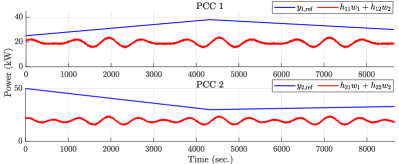
Figure 1: Reference signal and overall contribution of the non-controllable loads at the point of common coupling.
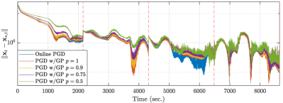
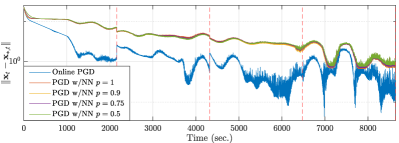
Figure 2: Error for different values of . (a) Learning with GPs. (b) Learning with feedforward NNs. In both cases, the blue line corresponds to the online algorithm with exact knowledge of .
We consider controllable DERs (accordingly, is the active power produced or consumed by the DER ), and PCCs. The power limits for the DERs are time-variant and change within the following bounds: kW, kW, and kW. The aggregate power of the non-controllable loads are shown in red in Figure 1, and the two demand response setpoints are color-coded in blue. The function is unknown; it is assumed that switches between two quadratic functions (with different coefficients), to reflect changes in the preferences of the DER-owners (switching times are represented by vertical red lines in Figure 2); for example, a DER owner can change preferences for the indoor temperature. We test two learning methods: (i) is estimated via GPs as explained in Section 4, and (ii) we use feedforward neural networks (NNs) to estimate the functions associated with the DERs. We evaluate the performance of the algorithm in (5) over a period equivalent to 12 hours, with each step of the algorithm performed every 5 seconds. We start to learn each of the users’ function with 5 noisy observations, and we collect functional evaluations from the DER owners every 30 minutes during the execution of the algorithm.
Figure 2(a) illustrates the performance of the online method when GPs are utilized (we use the labels “PGD w/GP”), averaged over experiments. For each experiment, we use a fixed step size and a random initial point . We show the mean error for four values of the Bernoulli parameter ; for comparison purposes, we run the online proximal gradient method with exact knowledge of (labeled as “online PGD”). The tracking error decreases linearly and then settles to a range of values that depend on as expected. It can also be seen that, when , the red trajectory and the blue one are very close after steps, indicating that the GP approximates well the function . Figure 2(b) presents the case when is learned via a feedforward NNs with one hidden layer of size 10 (labeled as “PGD w/NN”). The online algorithm exhibits a similar behavior; however, the tracking error is in general higher compared to the case where we use GPs. One reason for this behavior is the higher error in the gradient estimation; while GPs offer a closed-form expression for the gradient of the posterior mean, in the case of the NNs we estimated the gradient via centered difference.
6 Conclusions
We considered a feedback-based projected gradient method to solve a time-varying optimization problem associated with a system modeled with an algebraic map. The algorithm relies on inaccurate gradient information and exhibits random updates. We derived bounds for the error between the iterate of the algorithm and the optimal solution of the optimization problem in expectation and in high probability, by modeling gradient errors as sub-Weibull rvs and missing measurements as Bernoulli rvs. We established a connection with results in the context of ISS in expectation and in high probability for discrete-time stochastic dynamical systems.
References
[1]
A. Hauswirth, S. Bolognani, G. Hug, and F. Dörfler, “Optimization
algorithms as robust feedback controllers,” arXiv preprint
arXiv:2103.11329, 2021.
[2]
S. Bolognani and S. Zampieri, “A distributed control strategy for reactive
power compensation in smart microgrids,” IEEE Trans. on Automatic
Control, vol. 58, no. 11, pp. 2818–2833, 2013.
[3]
A. Bernstein, E. Dall’Anese, and A. Simonetto, “Online primal-dual
methods with measurement feedback for time-varying convex optimization,”
IEEE Trans. on Signal Processing, vol. 67, no. 8, pp. 1978–1991,
2019.
[4]
M. Vladimirova, S. Girard, H. Nguyen, and J. Arbel, “Sub‐weibull
distributions: Generalizing sub‐gaussian and sub‐exponential properties
to heavier tailed distributions,” Stat, vol. 9, no. 1, Jan 2020.
[5]
C. E. Rasmussen, “Gaussian processes for machine learning,” in Gaussian
processes for machine learning. MIT
Press, 2006.
[6]
I. Notarnicola, A. Simonetto, F. Farina, and G. Notarstefano, “Distributed
personalized gradient tracking with convex parametric models,” IEEE
Transactions on Automatic Control, 2022.
[7]
T. Hastie, R. Tibshirani, and J. Friedman, The elements of statistical
learning. Springer, 2009.
[8]
M. Marchi, J. Bunton, B. Gharesifard, and P. Tabuada, “Safety and stability
guarantees for control loops with deep learning perception,” IEEE
Control Systems Letters, vol. 6, pp. 1286–1291, 2022.
[9]
A. Simonetto, E. Dall’Anese, J. Monteil, and A. Bernstein, “Personalized
optimization with user’s feedback,” Automatica, vol. 131, p.
109767, 2021.
[10]
F. Fabiani, A. Simonetto, and P. J. Goulart, “Learning equilibria with
personalized incentives in a class of nonmonotone games,” arXiv
preprint arXiv:2111.03854, 2021.
[11]
S. Munir, J. A. Stankovic, C.-J. M. Liang, and S. Lin, “Cyber physical system
challenges for human-in-the-loop control,” in International Workshop
on Feedback Computing, 2013.
[12]
L. Lindemann, A. Robey, L. Jiang, S. Tu, and N. Matni, “Learning robust output
control barrier functions from safe expert demonstrations,” arXiv
preprint arXiv:2111.09971, 2021.
[13]
R. Vershynin, High-dimensional probability: An introduction with
applications in data science. Cambridge University press, 2018.
[14]
C.-Y. Chang, M. Colombino, J. Cortés, and E. Dall’Anese, “Saddle-flow
dynamics for distributed feedback-based optimization,” IEEE Control
Systems Letters, vol. 3, no. 4, pp. 948–953, 2019.
[15]
K. Hirata, J. P. Hespanha, and K. Uchida, “Real-time pricing leading to
optimal operation under distributed decision makings,” in American
Control Conference, 2014, pp. 1925–1932.
[16]
M. Colombino, J. W. Simpson-Porco, and A. Bernstein, “Towards robustness
guarantees for feedback-based optimization,” in IEEE Conference on
Decision and Control, 2019, pp. 6207–6214.
[17]
Y. Tang, K. Dvijotham, and S. Low, “Real-time optimal power flow,” IEEE
Trans. on Smart Grid, vol. 8, no. 6, pp. 2963–2973, 2017.
[18]
A. M. Ospina, A. Simonetto, and E. Dall’Anese, “Time-varying optimization of
networked systems with human preferences,” arXiv preprint
arXiv:2103.13470, 2021.
[19]
S. Liu, X. Li, P.-Y. Chen, J. Haupt, and L. Amini, “Zeroth-order stochastic
projected gradient descent for nonconvex optimization,” in IEEE
GlobalSIP, 2018, pp. 1179–1183.
[20]
Y. Tang, J. Zhang, and N. Li, “Distributed zero-order algorithms for nonconvex
multiagent optimization,” IEEE Trans. on Control of Network Systems,
vol. 8, no. 1, pp. 269–281, 2020.
[21]
D. D. Selvaratnam, I. Shames, J. H. Manton, and M. Zamani, “Numerical
optimisation of time-varying strongly convex functions subject to
time-varying constraints,” in IEEE Conference on Decision and
Control, 2018, pp. 849–854.
[22]
A. Mokhtari, S. Shahrampour, A. Jadbabaie, and A. Ribeiro, “Online
optimization in dynamic environments: Improved regret rates for strongly
convex problems,” in IEEE Conference on Decision and Control, 2016,
pp. 7195–7201.
[23]
G. Behrendt and M. Hale, “Technical report: A totally asynchronous algorithm
for tracking solutions to time-varying convex optimization problems,”
arXiv preprint arXiv:2110.06705, 2021.
[24]
N. Bastianello, L. Madden, R. Carli, and E. Dall’Anese, “A stochastic operator
framework for inexact static and online optimization,” arXiv preprint
arXiv:2105.09884, 2021.
[25]
E. Ryu and S. Boyd, “A primer on monotone operator methods survey,”
Applied and computational mathematics, vol. 15, pp. 3–43, 01 2016.
[26]
A. R. Teel, J. P. Hespanha, and A. Subbaraman, “Equivalent characterizations
of input-to-state stability for stochastic discrete-time systems,”
IEEE Trans. on Automatic Control, vol. 59, no. 2, pp. 516–522, 2013.
[27]
Z.-P. Jiang and Y. Wang, “Input-to-state stability for discrete-time nonlinear
systems,” Automatica, vol. 37, no. 6, pp. 857–869, 2001.
[28]
A. Lesage-Landry and D. S. Callaway, “Dynamic and distributed online convex
optimization for demand response of commercial buildings,” IEEE
Control Systems Letters, 2020.
Proof of Theorem 1. The proof of the theorem utilizes the definition of sub-Weibull rv in Definition 1(ii). To derive the main result, it is first necessary to characterize the rv , where and , . We will find the parameters and s.t. can be modeled as . By definition, is a binomial rv, i.e., since it is the sum of Bernoulli trials. Further, , which implies that is a bounded rv. Hence, we can model as a sub-Gaussian rv [13] and, thus, a sub-Weibull with .
Regarding , by the definition of the -th moment of a rv, we have that the -th moment of the bounded rv is
where (a) follows by the definition of expected value and probability mass function of the binomial rv; and, (b) uses the binomial identity. Thus,
(9)
We can see from (9) that the -th moment of , for a fixed , decays to zero as . On the other hand, if we fix a finite , we have that as . By Definition 1(ii) of the sub-Weibull rv, we have that
Therefore, is a decreasing function of , and it takes values in the set ; also, for . Thus, for any given and any finite , we can choose .
With this characterization in place, we now derive a bound for . Notice that satisfies the fixed-point equation . Then,
(10)
where (a) holds by (5); (b) by adding and subtracting ; (c) by reorganizing terms, using the triangle inequality, and the non-expansiveness property of the projection operator into the second term; (d) by using the triangle inequality on the second term, using the fact that is -Lipschitz, and the non-expansiveness property of the projection; and, (e) holds by adding and subtracting , using the triangle inequality, by the definition of , and .
To show 1(i), take the expectation of (10) to obtain
(11)
where (a) holds by the linearity of the expected value; (b) by the independence of the rvs and ; and, (c) holds by the expected value of the Bernoulli rv , where we also used . Recursively applying (11), we have,
Define the sub-sequence with for ; i.e., are the indices of the iterations where an update is performed. Then,
By definition of , between the times and the total number of updates is ; then, we rewrite (13) as follows:
(14)
where terms are added to the sum to remove the dependence on . Recall that , where is monotonically decreasing. By Assumptions 4-5 and Lemma 1, we have that ,
where and . Then, using Proposition 2, we get:
where ,
,
and where we used the closure of the sub-Weibull rv with respect to sum and product (with a scalar), and then the inclusion property.
To characterize the last term of (14) we have that
Note that is the sum of a given number of the deterministic path lengths ; then we get
(15)
The geometric rv can be characterized as a sub-Weibull rv. Since the exponential distribution is the continuous analogue of geometric distribution, and by logarithmic properties, we have ; by Proposition 2, we have that (15) . Therefore, (14) follows a sub-Weibull distribution with parameters and . Using the high probability bound (3) in Proposition 3 the result follows.