The role of neutral hydrogen in setting the abundances of molecular species in the Milky Way’s diffuse interstellar medium. I. Observational constraints from ALMA and NOEMA

Abstract

We have complemented existing observations of H I absorption with new observations of HCO⁺, C₂H, HCN, and HNC absorption from the Atacama Large Millimeter/submillimeter Array (ALMA) and the Northern Extended Millimeter Array (NOEMA) in the direction of 20 background radio continuum sources with $4^{\circ}\leq|b|\leq 81^{\circ}$ to constrain the atomic gas conditions that are suitable for the formation of diffuse molecular gas. We find that these molecular species form along sightlines where $A_{V}\gtrsim 0.25$, consistent with the threshold for the H I-to-H₂ transition at solar metallicity. Moreover, we find that molecular gas is associated only with structures that have an H I optical depth $>0.1$, a spin temperature $<80$ K, and a turbulent Mach number $\gtrsim 2$. We also identify a broad, faint component to the HCO⁺ absorption in a majority of sightlines. Compared to the velocities where strong, narrow HCO⁺ absorption is observed, the H I at these velocities has a lower cold neutral medium (CNM) fraction and negligible CO emission. The relative column densities and linewidths of the different molecular species observed here are similar to those observed in previous experiments over a range of Galactic latitudes, suggesting that gas in the solar neighborhood and gas in the Galactic plane are chemically similar. For a select sample of previously-observed sightlines, we show that the absorption line profiles of HCO⁺, HCN, HNC, and C₂H are stable over periods of $\sim 3$ years and $\sim 25$ years, likely indicating that molecular gas structures in these directions are at least $\gtrsim 100$ AU in size.

1 Introduction

The formation of molecular gas in the diffuse interstellar medium (ISM) marks the first stages of molecular cloud formation and interstellar chemistry. A variety of processes are believed to mediate molecule formation, including, for example, shielding (Krumholz et al., 2009; Sternberg et al., 2014), shock-driven turbulence (Inoue & Inutsuka, 2012), and turbulent dissipation (Godard et al., 2009; Lesaffre et al., 2020), but the relative importance of these different effects remains uncertain, from both observational and theoretical perspectives.

Molecular gas forms within the turbulent, multi-phase atomic ISM. Since at least the early work of Pikel’Ner (1968) and Field et al. (1969), it has been understood that atomic hydrogen (H I) can exist in a warm, diffuse phase (the warm neutral medium, WNM) and a cold, clumpy phase (the cold neutral medium, CNM). The WNM and CNM have been well characterized theoretically (Wolfire et al., 2003) and observationally in the case of the Milky Way (Heiles & Troland, 2003; Murray et al., 2018). However, observations have also established that $\sim 20\%$ of the H I in the Milky Way is in a thermally unstable phase (the unstable neutral medium, UNM), with intermediate temperature and density (Murray et al., 2018). Hydrodynamical and magnetohydrodynamical simulations have shown that CNM structures can form out of the diffuse WNM as the result of dynamical processes like shocks (Koyama & Inutsuka, 2002; Hennebelle & Audit, 2007; Inoue & Inutsuka, 2012). Thermal instabilities in shocked gas lead to the condensation of CNM structures with densities several orders of magnitude higher than typical WNM densities. The smallest ($\lesssim 0.1$ pc) and densest of these structures may represent tiny scale atomic structure (Hennebelle & Audit, 2007; Rybarczyk et al., 2020), an overdense, overpressured component of the atomic ISM observed in high resolution H I absorption measurements (“TSAS”; Heiles, 1997; Stanimirović & Zweibel, 2018, and references therein). Theoretical predictions suggest that molecular hydrogen (H₂) forms if the H I piled up behind a shock reaches a sufficiently high column density (Inutsuka et al., 2015) and the gas stays cold (Heitsch et al., 2006), although this depends on the metallicity (e.g., Bolatto et al., 2011) and the orientation of the local magnetic field with respect to the shock motion (Inoue & Inutsuka, 2012). The H I-to-H₂ transition—where a large fraction of atomic hydrogen is converted to molecular hydrogen—has been observed to occur at a total column density $N\gtrsim 5\times 10^{20}$ $\,{\rm cm^{-2}}$ at solar metallicity (Savage et al., 1977).

While it is clear that the turbulent, multi-phase ISM is an important ingredient for the formation and survival of molecules, it is still not understood how local properties of H I affect the molecular fraction. Several recent studies have provided hints that underlying physical properties of the H I, such as the level of turbulence and the presence of thermally unstable H I, play an important role. Observationally, Stanimirović et al. (2014) and Nguyen et al. (2019) showed that molecular clouds are embedded within atomic gas that has a high CNM fraction relative to random diffuse regions. By modeling the H I-to-H₂ transition in Perseus, Bialy et al. (2015) found that a mixture of CNM and UNM (and perhaps WNM) gas was important in controlling the H I-to-H₂ transition. The width of the transition regions between warm H I, cold H I, and cold H₂—and therefore the local properties of the H I-to-H₂ transition—also depends on the level of turbulence (Bialy et al., 2017; Lesaffre et al., 2007), and turbulent mixing between the WNM and CNM can enhance the formation of certain molecular species (Lesaffre et al., 2007; Glover & Clark, 2012).

In this work, we investigate the early stages of molecule formation in the diffuse ISM and connect this with the underlying properties of atomic gas using new absorption line observations of HCN, C₂H, HCO⁺, and HNC in the direction of 20 background radio continuum sources where the 21-SPONGE project (21 cm Spectral Line Observations of Neutral Gas with the Karl G. Jansky Very Large Array; Murray et al., 2015, 2018) previously observed H I in emission and absorption. In Section 2, we present these observations obtained using the Atacama Large Millimeter/submillimeter Array (ALMA) and the Northern Extended Millimeter Array (NOEMA), along with existing observations in these directions, including observations of H I emission from the Arecibo Observatory and H I absorption from the Very Large Array (VLA) obtained by the 21-SPONGE project (Murray et al., 2015, 2018), maps of interstellar redenning and dust temperature from the Planck satellite (Planck Collaboration et al., 2014a, b), and observations of CO emission from the Dame et al. (2001) survey. 21-SPONGE targeted mainly sources at Galactic latitude $>10^{\circ}$, where H I spectra are simpler and radiative transfer calculations are easier than in the Galactic plane. The sensitivity of our molecular line spectra rival or exceed most pre-ALMA surveys (e.g., Lucas & Liszt, 1996, 2000; Liszt & Lucas, 2001), and our sample represents one of the largest homogeneous samples of Galactic absorption measurements at mm wavelengths to date. We outline methods for extracting molecular column densities and decomposing absorption spectra into Gaussian components in Section 3. In Section 4, we test how the observed molecular column densities depend on the line of sight gas properties, including the extinction and the CNM and UNM column densities. We also investigate a broad, faint component of the HCO⁺ absorption seen in the direction of most background sources. In Section 5, we establish thresholds for the H I optical depth, spin temperature, and turbulent Mach number required for the onset of molecule formation. We then determine the relative abundances and linewidths of the four different molecular species observed in this work and compare our results with previous works in Section 6. In Section 7, we investigate the temporal stability of absorption line profiles by comparing our results to previous observations of HCN, C₂H, HCO⁺, and HNC for select lines of sight. This serves as a probe for AU scale structure. Finally, we discuss our results in Section 8 and present conclusions in Section 9.

This is the first of two complementary papers. In Rybarczyk et al. (submitted; Paper II hereafter) we compare the observational results presented here to predictions from the Gong et al. (2017) photodissociation region (PDR) chemical model and the Gong et al. (2020) ISM simulations.

2 Observations

Table 1: The molecular line transitions covered by the ALMA-SPONGE spectral setup. HCN and HCO⁺ were also covered by the NOEMA-SPONGE spectral setup. Column 1 lists the molecular species. Column 2 lists each transition. Column 3 lists the rest frequency for each transition. Column 4 gives the conversion between the optical depth integral and the column density for each species (see Section 3.1); the values listed in Column 4 account for all of the observed transitions for each species and are calculated assuming an excitation temperature equal to the CMB temperature, 2.725 K.

Species	Transition	Frequency	$N/\int\tau dv$
		GHz	$\,{\rm cm^{-2}}$/$\,{\rm km\,s^{-1}}$
C2H	$N=1-0$ $J=3/2-1/2$ $F=2-1$	$87.3169$	$4.34\times 10^{13}$
C2H	$N=1-0$ $J=3/2-1/2$ $F=1-0$	$87.3286$
HCN	$J=1-0$ $F=1-1$	$88.6304$	$1.91\times 10^{12}$
HCN	$J=1-0$ $F=2-1$	$88.6318$
HCN	$J=1-0$ $F=0-1$	$88.6339$
HCO+	$J=1-0$	$89.1890$	$1.11\times 10^{12}$
HNC	$J=1-0$	$90.6336$	$1.78\times 10^{12}$

2.1 Observations with ALMA (ALMA-SPONGE)

We have observed C₂H, HCN, HCO⁺, and HNC in absorption with ALMA during observing Cycles 6 and 7 (ALMA-SPONGE projects 2018.1.00585.S and 2019.1.01809.S, PI: Stanimirovic) in the direction of 20 bright background radio continuum sources previously observed at 21 cm wavelength using the VLA by the 21-SPONGE project. Observations were obtained between October 2018 and March 2020. The transitions covered by our observations are listed in Table 1. 89 GHz fluxes ranged from 0.03 Jy to 11.8 Jy. The HCO⁺ and HNC spectra were obtained at 30.5 kHz frequency channel spacing (0.1 $\,{\rm km\,s^{-1}}$ velocity channel spacing) while the HCN and C₂H spectra were obtained at 61 kHz frequency channel spacing (0.2 $\,{\rm km\,s^{-1}}$ velocity channel spacing). In the analysis that follows, all spectra have been smoothed to $0.4$ $\,{\rm km\,s^{-1}}$ velocity resolution, comparable to that of the 21-SPONGE H I absorption spectra.

With the exception of 3C111 and 3C123, all of the ALMA-SPONGE background radio continuum sources are unresolved and treated as single point sources. 3C111 is a three-component radio galaxy; we have independent observations of all three components, separated by $1\arcmin$–$3\arcmin$, each of which is unresolved. Although the 1420 MHz fluxes vary by less than a factor of 3 across the three components, the 89 GHz fluxes change by over two orders of magnitude. We do not consider the spectra in the direction of 3C111C hereafter, as they lack adequate sensitivity to accurately measure molecular abundances ($\sigma_{\tau}\gtrsim 1$). The optical depth noise of the C₂H and HNC spectra are $\sim 0.3$ for 3C111B, the highest in our sample. As discussed in the next section, we have obtained more sensitive HCO⁺ and HCN absorption spectra in the direction of 3C111A and 3C111B with NOEMA. 3C123 is also a multiple-component continuum source. Murray et al. (2018) resolved 3C123 into two components, 3C123A and 3C123B. At ALMA’s higher resolution, we resolve 3C123 into four components. Because we make a direct comparison between the 21-SPONGE H I absorption spectra and our molecular absorption spectra, though, we regrid our ALMA observations in the direction of 3C123 using the VLA beam (20.3″ $\times$ 5.3″) from the Murray et al. (2018) observations before extracting the absorption spectra. As in Murray et al. (2018), we resolve only two components at this lower spatial resolution, which are here referred to as 3C123A and 3C123B to be consistent with their labeling. While the spectra toward 3C123A have a typical optical depth noise of 0.01, the optical depth noise in the 3C123B spectra is $\sim 0.1$.

For sources without significant absorption, we extracted the spectra from the continuum-subtracted data cubes output by the default ALMA Science Pipeline at the pixel of peak continuum flux. To calculate upper limits to the optical depth, we added the continuum flux back to the continuum-subtracted spectra (correcting for the spectral index; for a majority of sightlines, the continuum is relatively flat). For sightlines that showed significant absorption, we reran the ALMA Science Pipeline without continuum subtraction and extracted spectra from the pixel of peak continuum flux to ensure the most reliable estimate of the continuum flux and the optical depths. Except in the cases noted above, at $0.4$ $\,{\rm km\,s^{-1}}$ velocity resolution, we reach a typical optical depth noise of $\sim 0.01$ in the ALMA-SPONGE spectra.

Table 2.3.2 lists the Galactic coordinates and integrated optical depths in the direction of the 19 ALMA-SPONGE bright background radio continuum sources (excluding 3C111C). 10 sightlines show no molecular absorption at a level of $3\sigma$. 6 sightlines show strong absorption across all four molecular species. In the direction of 3C111B, we detect HNC absorption but no C₂H absorption (HCO⁺ and HCN are observed with NOEMA; see next section). This most likely reflects the poor sensitivity in the direction of 3C111B—the peak C₂H optical depth in the direction of 3C111A is 0.766, which is only 2.6 times the noise level in the 3C111B spectrum. In the direction of 3C78, we see weak HCO⁺ absorption, but no HCN, C₂H, or HNC absorption. In the direction of J2136, we see weak C₂H absorption, but no HCN, HCO⁺, or HNC absorption. Although the detections in the direction of 3C123B, 3C78, and J2136 are marginal ($\sim 3\sigma$), they appear significant at lower velocity resolution. Moreover, the absorption in these directions is aligned in velocity with H I absorption features. We also see two hyperfine components for J2136 and we know from the 3C123A spectra that molecular gas is present toward 3C123 at the velocities where we detect marginal absorption in the direction of 3C123B. The spatial distribution of all ALMA-SPONGE sources is shown in Figure 1, overlaid on a map of CO integrated emission measured by Planck Collaboration et al. (2014b).

2.2 Observations with NOEMA (NOEMA-SPONGE)

We observed HCO⁺ and HCN in absorption at 62.5 kHz channel spacing (0.2 $\,{\rm km\,s^{-1}}$ velocity spacing) with NOEMA (NOEMA-SPONGE, projects W19AQ and S20AB) in the direction of 3C111—both A and B components—and BL Lac. 3C111 was observed in January 2020 and BL Lac was observed October 2020. The measured fluxes were 1.13 Jy for 3C111A, 0.06 Jy for 3C111B, and 2.10 Jy for BL Lac. Both HCO⁺ and HCN were placed in high resolution chunks in the lower side band, which was tuned to 90 GHz. Standard calibration was carried out using the CLIC and MAPPING software, part of the GILDAS software collection (Pety, 2005; Gildas Team, 2013). Because BL Lac and 3C111A were bright, we further performed self-calibration using the 2020 Self Calibration tool in MAPPING. We smooth the final spectra to 0.4 $\,{\rm km\,s^{-1}}$ velocity resolution, reaching an optical depth sensitivity of $\sim 0.002$ for 3C111A and BL Lac and an optical depth sensitivity of $\sim 0.05$ for 3C111B. The NOEMA-SPONGE sensitivity in the direction of 3C111B is significantly better than the ALMA-SPONGE sensitivity; only the NOEMA-SPONGE HCO⁺ and HCN data in this direction are considered hereafter. The HCO⁺ and HCN optical depth integrals in these directions are listed in Table 2.3.2 (where the NOEMA-SPONGE fluxes are superscripted by a “1”) and their positions are shown in Figure 1.

2.3 Additional data sets

2.3.1 21-SPONGE

The 21-SPONGE project (Murray et al., 2015, 2018) obtained H I absorption spectra using the VLA and H I emission spectra using the Arecibo Observatory in the direction of 57 bright background radio continuum sources, ranging in latitude from $|b|=3.7^{\circ}$ to $|b|=81^{\circ}$. The absorption spectra had an optical depth noise of $\sim 10^{-3}$ at the 0.4 $\,{\rm km\,s^{-1}}$ velocity resolution. Murray et al. (2015, 2018) decomposed the absorption and emission spectra into Gaussian components. They estimated the spin temperatures, $T_{S}$, and H I column densities, $N({\rm H\,{\small I}}{})$, of the H I structures seen in absorption. They also investigated the fraction of gas in the CNM, the WNM, and the UNM phases along each line of sight. We use their absorption spectra and adopt their Gaussian fits in this work. The 21-SPONGE H I absorption spectra are shown in Figure 2.

2.3.2 $E(B-V)$ and $T_{d}$ from Planck

The total hydrogen column density, $N_{\mathrm{H}}=N({\rm H\,{\small I}}{})+2N(\text{H\textsubscript{2}}{})$, can be inferred from the interstellar reddening, $E(B-V)$, along the line of sight. We use the dust radiance, $\mathcal{R}$, measured by Planck to estimate $E(B-V)$. $\mathcal{R}$ is a more reliable predictor of $E(B-V)$ than the 353 µm optical depth, $\tau_{353}$, at high Galactic latitude (Planck Collaboration et al., 2014a). We extract $E(B-V)$ at the pixel nearest to each background source using the dustmaps Python package (Green, 2018). The Planck dust maps have a resolution of 5′ and a typical fractional uncertainty of $\sim 10\%$ in $E(B-V)$. The results are listed in Table 2.3.2. We also extract the dust temperature, $T_{d}$, derived by Planck Collaboration et al. (2016) using the generalized needlet internal linear combination (GNILC) method and a modified blackbody spectral model on Planck temperature maps at 353, 545, 857, and 3000 GHz. We use dust temperature as a proxy for the strength of the interstellar radiation field (ISRF)—the strength of the FUV radiation field scales as $T_{d}^{\beta+4}$, where $\beta$ is the power law index characterizing the dust emissivity cross-section as a function of frequency (see Equation 7.15 of Lequeux, 2005). To estimate the ISRF we also extract the corresponding $\beta$ values at each of our positions.

In several places in this paper we use values of $E(B-V)$, $T_{d}$, and the ISRF derived from Planck as estimates of the gas properties along the lines of sight. While this provides a uniform approach, because Planck’s resolution is much lower than that of our H I and molecular pencil-beam absorption spectra, we consider these only as rough estimates and not precise measures of the local physical conditions.

Table 2: Observed properties of the sightlines in this study. Col. 1: Name of the background radio continuum source. Col. 2: The 90 GHz continuum flux. Col. 3: Galactic longitude and latitude of the background source in degrees. Col. 4: Total H I column density measured by 21-SPONGE along the line of sight (Murray et al., 2018). Col. 5: $E(B-V)$ inferred from the dust radiance measured by Planck (Planck Collaboration et al. 2014). Cols. 6–9: The integrated optical depth for all four species for channels with $\tau>3\sigma_{\tau}$. Lower limits are indicated. As described in Section 2, BL Lac was not observed in C₂H or HNC absorption.

Source	$F_{90}$	$l/b$	$N({{\rm H\,{\small I}}{}})$	$E(B-V)$	$\int\tau_{\text{HCN}}{}dv$	$\int\tau_{\text{C\textsubscript{2}H}}{}dv$	$\int\tau_{\text{HCO\textsuperscript{+}}}{}dv$	$\int\tau_{\text{HNC}}{}dv$
	$\rm{Jy}$	∘	$10^{20}$ $\,{\rm cm^{-2}}$	mag	$\,{\rm km\,s^{-1}}$	$\,{\rm km\,s^{-1}}$	$\,{\rm km\,s^{-1}}$	$\,{\rm km\,s^{-1}}$
3C154	0.390	$185.6$/$4.0$	$37.12$	$0.425$	$3.325\pm 0.039$	$1.079\pm 0.025$	$3.059\pm 0.056$	$0.819\pm 0.023$
3C111A	0.769/1.1451	$161.7$/$-8.8$	$25.96$	$0.827$	$>12.710$	$2.057\pm 0.033$	$>11.054$	$3.606\pm 0.129$
3C111B	0.034/0.0601	$161.7$/$-8.8$	$24.86$	$0.827$	$>11.345$	$\cdot\cdot\cdot$	$>6.780$	$>2.028$
BLLac	2.189	$92.6$/$-10.4$	$18.68$	$0.350$	$4.316\pm 0.007$		$2.546\pm 0.002$
3C138	0.470	$187.4$/$-11.3$	$20.51$	$0.263$	$\cdot\cdot\cdot$	$\cdot\cdot\cdot$	$\cdot\cdot\cdot$	$\cdot\cdot\cdot$
3C123A	0.451	$170.6$/$-11.7$	$17.33$	$0.499$	$6.029\pm 0.171$	$1.650\pm 0.041$	$6.280\pm 0.234$	$1.100\pm 0.041$
3C123B	0.270	$170.6$/$-11.7$	$18.66$	$0.499$	$>4.287$	$0.331\pm 0.189$	$>4.071$	$1.222\pm 0.965$
PKS0742	0.304	$209.8$/$16.6$	$3.37$	$0.031$	$\cdot\cdot\cdot$	$\cdot\cdot\cdot$	$\cdot\cdot\cdot$	$\cdot\cdot\cdot$
3C120	2.431	$190.4$/$-27.4$	$13.33$	$0.275$	$0.031\pm 0.003$	$0.178\pm 0.006$	$0.283\pm 0.006$	$0.006\pm 0.002$
J2136	2.063	$55.5$/$-35.6$	$4.34$	$0.080$	$\cdot\cdot\cdot$	$0.012\pm 0.002$	$\cdot\cdot\cdot$	$\cdot\cdot\cdot$
3C346	0.107	$35.3$/$35.8$	$5.42$	$0.082$	$\cdot\cdot\cdot$	$\cdot\cdot\cdot$	$\cdot\cdot\cdot$	$\cdot\cdot\cdot$
3C454.3	11.838	$86.1$/$-38.2$	$7.03$	$0.117$	$0.112\pm 0.004$	$0.106\pm 0.004$	$0.276\pm 0.004$	$0.024\pm 0.002$
3C345	2.489	$63.5$/$40.9$	$0.75$	$0.021$	$\cdot\cdot\cdot$	$\cdot\cdot\cdot$	$\cdot\cdot\cdot$	$\cdot\cdot\cdot$
4C15.05	0.596	$147.9$/$-44.0$	$4.06$	$0.057$	$\cdot\cdot\cdot$	$\cdot\cdot\cdot$	$\cdot\cdot\cdot$	$\cdot\cdot\cdot$
3C78	0.347	$174.9$/$-44.5$	$10.65$	$0.162$	$\cdot\cdot\cdot$	$\cdot\cdot\cdot$	$0.043\pm 0.012$	$\cdot\cdot\cdot$
1055+018	5.283	$251.5$/$52.8$	$3.05$	$0.037$	$\cdot\cdot\cdot$	$\cdot\cdot\cdot$	$\cdot\cdot\cdot$	$\cdot\cdot\cdot$
3C273	8.668	$289.9$/$64.4$	$2.16$	$0.028$	$\cdot\cdot\cdot$	$\cdot\cdot\cdot$	$\cdot\cdot\cdot$	$\cdot\cdot\cdot$
4C12.50	0.507	$347.2$/$70.2$	$2.18$	$0.054$	$\cdot\cdot\cdot$	$\cdot\cdot\cdot$	$\cdot\cdot\cdot$	$\cdot\cdot\cdot$
3C286	0.671	$56.5$/$80.7$	$1.21$	$0.016$	$\cdot\cdot\cdot$	$\cdot\cdot\cdot$	$\cdot\cdot\cdot$	$\cdot\cdot\cdot$
4C32.44	0.229	$67.2$/$81.0$	$1.36$	$0.021$	$\cdot\cdot\cdot$	$\cdot\cdot\cdot$	$\cdot\cdot\cdot$	$\cdot\cdot\cdot$

¹ As described in Section 2, 3C111A and 3C111B were observed by both ALMA (C₂H, HNC) and NOEMA (HCN, HCO⁺); both fluxes are listed, with the flux for the NOEMA data superscripted by a “1.”

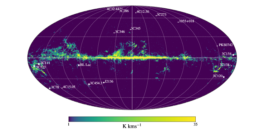
Figure 1: The distribution of background radio continuum sources observed in this work plotted over a full sky map of the CO integrated intensity from Planck Collaboration et al. (2014b). Sources with molecular absorption detections at a level $\geq 3\sigma$ are shown as filled stars; sources with no molecular absorption detections are shown as filled circles. The integrated intensity of the CO emission is shown with a logarithmic color scale, ranging from 1 K $\,{\rm km\,s^{-1}}$ to 35 K $\,{\rm km\,s^{-1}}$. The different components of the multiple-component continuum sources 3C111 and 3C123 are indistinguishable at this resolution so are not labeled separately (see Table 2.3.2). Dashed lines show Galactic latitude and longitude with $30^{\circ}$ spacing.

2.4 CO emission spectra from the CfA 1.2m telescope

Dame et al. (2001) obtained CO emission spectra across the entire Galactic plane and select clouds at higher latitudes using the CfA 1.2m telescope with a $8.4\arcmin$ beamwidth. For sources covered by this CO survey, we extract CO emission spectra from the nearest pixel in the Dame et al. (2001) maps, sampled between every other beamwidth ($0.25^{\circ}$) and every half beamwidth ($0.0625^{\circ}$) in the directions of our sources. The brightness temperature noise in these spectra ranges from 0.15 K to 0.30 K. For sources outside of the bounds covered by Dame et al. (2001), we use unpublished spectra obtained with the CfA 1.2m telescope at $8.4\arcmin$ beamwidth and $0.25^{\circ}$ sampling. The brightness temperature noise in these unpublished spectra is uniform, 0.18 K. All of the CO emission spectra taken from Dame et al. (2001) have a velocity resolution of $0.65$ $\,{\rm km\,s^{-1}}$.

3 Methods

3.1 Deriving Column Densities

For a ground state transition, the column density, $N$, and optical depth integral, $\int\tau dv$, for a particular species are related by

$$N=Q(T_{\mathrm{ex}})\frac{8\pi\nu^{3}}{c^{3}}\frac{1}{g_{u}A_{ul}}\Big{[}1-\exp(-h\nu/kT_{\mathrm{ex}})\Big{]}^{-1}\int\tau dv,$$ (1)

where $\nu$ is the frequency of radiation resulting from the transition from the upper state $u$ to the lower state $l$, $g_{u}$ is the degeneracy of the upper state, $A_{ul}$ is the Einstein $A$ coefficient for the transition, $T_{\mathrm{ex}}$ is the excitation temperature, and $Q(T_{\mathrm{ex}})$ is the partition function. We calculate $N/\int\tau dv$ using constants given in the Cologne Database for Molecular Spectroscopy (CDMS; Müller et al., 2001; Endres et al., 2016) and the Leiden Atomic and Molecular Database (LAMBDA; Schöier et al., 2010). For C₂H, we use $N/\int\tau dv=1.6\times 2.71\times 10^{13}$ $\,{\rm cm^{-2}}{}/\,{\rm km\,s^{-1}}{}$, provided by Lucas & Liszt (2000), where the factor of 1.6 accounts for the fact that we are measuring two of the six satellite C₂H lines. All values of $N/\int\tau dv$ are calculated assuming an excitation temperature is equal to the temperature of the CMB, 2.725 K (e.g., Godard et al., 2010; Luo et al., 2020). All conversions are listed in Table 1; the C₂H and HCN conversions account for all hyperfine transitions listed in Table 1.

For saturated channels where the measured value of $I(v)\leq 0$—and therefore $\tau(v)$ is infinite—we define the optical depth lower limit to be

$$\tau_{ll}(v)=-\ln\Big{(}\frac{2\sigma_{I}}{I_{0}}\Big{)},$$ (2)

where $\sigma_{I}$ is the noise in the spectrum of specific intensity. We then calculate a lower limit to the column density (Equation 1) using $\tau(v)=\tau_{ll}(v)$ for the saturated channels. We note that this systematically underestimates the optical depth for spectra with saturated absorption. In the analysis that follows, we therefore consider the optical depths and column densities only for spectra where the absorption is not saturated, unless otherwise noted. The optical depth integrals for saturated absorption spectra in Table 2.3.2 should be considered as conservative lower limits.

In Section 4, we estimate the total hydrogen column density, $N_{\mathrm{H}}$, from the reddening, $E(B-V)$, according to Zhu et al. (2017),

$$N_{\mathrm{H}}=2.08\times 10^{21}\times 3.1E(B-V)\text{ }\mathrm{cm^{-2}\,mag^{-1}},$$ (3)

where $3.1E(B-V)$ is here used for the visual extinction, $A_{V}$. This estimate was derived from a compilation of Galactic sources with optical and X-ray observations, and is consistent with other previous estimates (Jenkins & Savage, 1974; Bohlin et al., 1978; Krumholz et al., 2009; Rachford et al., 2009a) for sources spanning a wide range of Galactic latitudes and $N_{\mathrm{H}}$. Nevertheless, the ratio of $N_{\mathrm{H}}$ to $E(B-V)$ is not universal, and contributes additional uncertainty to the determination of $N_{\mathrm{H}}$—see Section 6 for discussion.

3.2 Gaussian Decomposition

We decompose the molecular optical depth spectra into Gaussian functions,

$$\tau(v)=\sum_{i=1}^{M}\tau_{i}(v)=\sum_{i=1}^{M}\tau_{0,i}e^{-4\ln{2}(v-v_{0,i})^{2}/\Delta v_{0,i}^{2}},$$ (4)

where $\tau_{0,i}$, $v_{0,i}$, and $\Delta v_{0,i}$ are the peak optical depth, the central velocity, and the full width at half maximum (FWHM) of the $i$^th Gaussian component, respectively, and there are $M$ Gaussian functions fit to the optical depth spectrum. Lucas, Liszt, Gerin, and collaborators have identified dozens of molecular absorption components in common across various molecular species, including HCN, C₂H, HCO⁺, and HNC. Further, they have found that the central velocities of absorption components identified at these transitions are nearly identical, and that FWHMs vary across different species by only $\sim 10$–$30\%$. Therefore, for each line of sight, we find the best solution to Equation 4 for the C₂H, HCN, HCO⁺, and HNC optical depth spectra using Python’s scipy.optimize.curve_fit from sets of initial guesses with the same number of components (modulo an integer factor accounting for the number of hyperfine transitions). The initial guesses for the FWHM and central velocity of each component are the same for all four optical depth spectra. The initial guesses for the central velocities of the different hyperfine C₂H and HCN components are offset according to the known frequency separation of the transitions, and the initial guesses for the optical depths are scaled to the LTE ratios ($2:1$ and $5:3:1$, respectively). For 3C111B and 3C123B, we use the same initial guesses at 3C111A and 3C123A, where the spectra are more sensitive. When fitting, we allow the peak optical depths to freely vary, the FWHMs to vary by a factor of two from the initial guess, and the central velocity to vary by $\pm 1$ $\,{\rm km\,s^{-1}}$ from the initial guess. Only solutions with peak optical depths $>3\sigma_{\tau}$ are classified as detections. For C₂H and HCN, we require only that the strongest transition be detected at a level of $3\sigma$.

The Gaussian-fitted components to the absorption spectra are shown in Figure 2. Tables 9, 9, 9, and 9 list the fits for C₂H, HCN, HCO⁺, and HNC, respectively. Peak optical depths range between $0.008$ and $2.5$, excluding saturated lines with optical depths $\gtrsim 3.5$. FWHMs range between $0.5$ $\,{\rm km\,s^{-1}}$ and $3.4$ $\,{\rm km\,s^{-1}}$. For 10 sightlines, no features are detected (see Table 2.3.2). There is one feature identified in C₂H absorption in the direction of J2136 for which there is no corresponding HCN, HCO⁺, or HNC absorption; and there is one feature identified in HCO⁺ absorption in the direction of 3C78 for which there is no corresponding HCN, C₂H, or HNC absorption. Two features are seen in C₂H and HCO⁺ absorption but not seen in HNC or HCN absorption. Three absorption features identified in C₂H, HCO⁺, and HCN are not detected in HNC.

Figure 2:

Figure 2:

Figure 2: The optical depth spectra, $e^{-\tau}$, versus LSR velocity for H I (bottom, black; Murray et al., 2018), HCO⁺ (second from bottom, red), HCN (middle, blue), HNC (second from top, gray), and C₂H (top, green). HCN velocities correspond to the $F=2-1$ transition. C₂H velocities correspond to the $F=2-1$ transition. The velocity of the $F=1-0$ C₂H transition has been shifted by $+25$ $\,{\rm km\,s^{-1}}$ for viewing convenience. Gaussian fits to the H I spectra from 21-SPONGE (Murray et al., 2018) and Gaussian fits to the molecular absorption spectra from this work (see Section 3.2) are shown as dashed lines. Absorption spectra that have been amplified are labeled with the multiplication factor.

4 Molecular gas in the diffuse ISM

The distribution of these background sources across the sky is shown in Figure 1, overlaid on the CO integrated intensity image from Planck Collaboration et al. (2014b). We show our ALMA/NOEMA observations of HCN, C₂H, HCO⁺, and HNC, as well as H I absorption from 21-SPONGE, in Figure 2. Table 2.3.2 summarizes the observational results in these directions, including the H I column density (Murray et al., 2018), reddening (Planck Collaboration et al., 2014a), and molecular optical depth integrals, calculated for channels with an optical depth $\tau(v)\geq 3\sigma_{\tau}$. Sources are listed in order of increasing Galactic latitude.

For most sources at latitudes $\lesssim 40^{\circ}$ degrees, we detect at least one of four transitions. For sources at latitude $>40^{\circ}$, we detect marginal HCO⁺ absorption along only one sightline, and no molecular absorption in any other direction. This is evident in Figure 1, where sources with molecular absorption detections are indicated using stars, while sources with no molecular detections are indicated using circles. There is no significant CO emission observed in the Planck Collaboration et al. (2014a) or Dame et al. (2001) data in the direction of three sightlines with molecular absorption detections—3C120, 3C78, and J2136. These sources have $|b|=27^{\circ}$–$44^{\circ}$. We discuss this further in Section 4.2.

The integrated optical depths—and therefore column densities (Equation 1)—span over two orders of magnitude across our sample for each of the molecular species, indicating that we are probing diverse interstellar environments. In Section 7, we compare the results in Table 2.3.2 to previous observations of HCN, C₂H, HCO⁺ and HNC in the same directions, taken between 3 and 25 years ago. All variations are at a level $\lesssim 3\sigma$, demonstrating that our observing and processing strategies are sound.

Figure 3: Molecular column densities versus visual extinction ($A_{V}$; upper left), H I CNM column density (upper right), H I UNM column density (lower left), and the combined column density of the CNM and UNM (lower right). Colors indicate the dust temperature derived by Planck Collaboration et al. (2016). Because the resolution of the Planck extinction maps is $5\arcmin$, the A and B components of 3C111 and 3C123 have the same $x$ coordinate in the upper left panel, so are not labeled separately.

4.1 Thresholds for molecule formation

In Figure 3, we compare the observed molecular column densities to the neutral and total gas column densities. The total gas column density is traced via the visual extinction ($A_{V}=3.1E(B-V)$; upper left). For the H I gas we investigate the CNM column density (the H I column density occupied by gas with $T_{S}<250$ K; upper right), the UNM column density, (the H I column density occupied by gas with $250\text{ K}<T_{S}<1000$ K; lower left), and the sum of the CNM and UNM column densities (lower right), for each line of sight. For non-detections, we show $3\sigma$ upper limits to the molecular column densities assuming a FWHM of 3 channels or 1.2 $\,{\rm km\,s^{-1}}$. The data points are color-coded based on the dust temperature provided by Planck, which can be used as a proxy for the ISRF.

The upper left panel of Figure 3 suggests a threshold visual extinction $A_{V}\approx 0.25$ below which no molecular absorption is detected and above which molecular abundances tend to increase with increasing $A_{V}$. A visual extinction $A_{V}\gtrsim 0.25$ corresponds to a total hydrogen column density $N_{\mathrm{H}}\gtrsim 5\times 10^{20}$ $\,{\rm cm^{-2}}$ (e.g., Güver & Özel, 2009; Zhu et al., 2017), which is roughly the threshold column density for the H I-to-H₂ transition at solar metallicity (e.g., Spitzer et al., 1973; Savage et al., 1977; Krumholz et al., 2009; Gong et al., 2018). Lucas & Liszt (1996) identified a similar threshold from observations of HCO⁺ (as well as OH), and Lucas & Liszt (2000) showed that C₂H was as widespread as HCO⁺. These results suggest that a similar column density threshold applies in the case of HCO⁺, HCN, HNC and C₂H. Essentially, as soon as conditions are suitable for H₂ survival, these other species follow quickly. The sightline toward 3C138, is an exception—it has a visual extinction of 0.815 but no detectable molecular absorption. This sightline is explored in greater depth in Section 8.5. The $A_{V}$ trend shown in this figure also follows the dust temperature distribution, again highlighting the importance of shielding against the radiation field. The five sources with the highest molecular column densities ($\gtrsim 10^{12}$ $\,{\rm cm^{-2}}$ for all four species) have the lowest dust temperature, $T_{d}\sim 17$ K, and FUV radiation field $G^{\prime}\sim 0.4$, where $G^{\prime}$ is the radiation field strength relative to the standard Draine (1978) field, calculated using $T_{d}$ and $\beta$ from Planck (see Section 2.3.2). The rest of the sources have molecular column densities $\lesssim 10^{12}$ cm^-2, $T_{d}\sim 19$ K, and have $G^{\prime}\sim 1$.

The lower left panel of Figure 3 shows the molecular column densities as a function of the column density of the thermally unstable H I. While this graph lacks a correlation, there is a clear dichotomy of sources: the sources with the highest molecular column densities ($>10^{12}$ cm^-2 for all species) all have $N({\rm H\,{\small I}}{})_{\mathrm{UNM}}\sim 10^{20-21}$ cm^-2, and the fraction of H I in the UNM is $\sim 30$–$70\%$ for these sightlines); all other sources have essentially no UNM gas. The only exception is 3C78, which has a high UNM column density and low molecular column densities. This suggests that UNM gas likely plays an important role for molecule formation and survival.

Meanwhile, in the two right panels of Figure 3, we see that there is a threshold of $\gtrsim 10^{20}$ $\,{\rm cm^{-2}}$ for the column density of cold H I below which no molecular absorption is detected (J2136—the only exception—is the lowest column density source to show molecular absorption, with $N({\rm H\,{\small I}}{})\approx 4\times 10^{19}$ $\,{\rm cm^{-2}}$ and very weak C₂H absorption). Again, this threshold is similar to the column density threshold for the H I-to-H₂ transition ($\sim 5\times 10^{20}$ $\,{\rm cm^{-2}}$ Savage et al., 1977). The correlation seen in the lower right plot, where the $x$-axis traces the total amount of cold H I, is qualitatively similar to that seen in the upper left plot, and again reflects the importance of shielding.

We do not see any difference here across the different chemical species probed in this study. For example, Goddard et al. (2014) suggested that HCO⁺ and C₂H are more sensitive to turbulent dissipation than HCN or HNC. We note, though, that our sample size is modest, and very few structures do not show absorption from all four species.

Figure 4: A comparison of the HCO⁺ optical depth (blue, positive) with H I absorption (red, negative, with Gaussian components shown as dahsed lines; Murray et al., 2018). Regions without HCO⁺ absorption are shaded in cross-hatched gray. Regions with weak, broad HCO⁺ absorption are shaded in diagonally-hatched green. Regions of strong, narrow HCO⁺ absorption are shaded in unhatched blue.

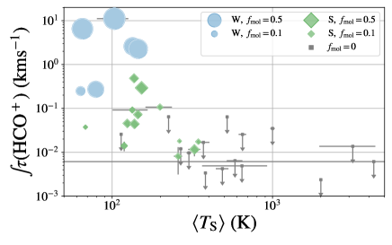
Figure 5: The integrated HCO⁺ optical depth versus the H I optical depth-weighted mean spin temperature in regions with strong HCO⁺ absorption (blue circles), weak HCO⁺ absorption (green diamonds), and no HCO⁺ absorption (gray points, shown as upper limits), as illustrated in Figure 4. The sizes of the plotted points correspond to the molecular fraction, $f_{\mathrm{mol}}=2N(\text{H\textsubscript{2}}{})/N_{\mathrm{H}}$, and the colors indicate the H I column densities.

4.2 A broad, faint component of HCO⁺ absorption

In addition to the narrow, strong absorption features easily identifiable in the spectra shown in Figure 2, we also detect a broad, faint component of HCO⁺ absorption in a majority of sightlines. Typical HCO⁺ optical depths are between 0.01 and 0.1 for the broad component, while narrow absorption lines have typical optical depths $>0.1$. In the direction of 3C111A, 3C120, and 3C123A, we detect HCO⁺ absorption across nearly all velocities where 21-SPONGE detected H I absorption (Figure 4). The HCO⁺ absorption in the direction 3C154 and BL Lac spans $\gtrsim 10$ $\,{\rm km\,s^{-1}}$, covering more than half of the velocity range where H I absorption is observed. In the direction of 3C454.3, the HCO⁺ absorption is localized mostly to a narrow range of velocities around $-10$ $\,{\rm km\,s^{-1}}$, but there are marginal detections at $v\approx-30$ $\,{\rm km\,s^{-1}}$ and $v\approx-15$ $\,{\rm km\,s^{-1}}$, where H I absorption is also observed. In the direction of 3C78, HCO⁺ absorption is weak, and confined only to a narrow velocity range compared to the H I absorption. Some of these broad features are fit with Gaussians, while some features are only apparent in the residuals (since they have peak optical depths $\lesssim 0.05$ and widths $\gtrsim 3\,{\rm km\,s^{-1}}{}$). We do not consider 3C111B or 3C123B here because of the relatively poor optical depth sensitivity in these directions.

4.2.1 Physical properties of the broad HCO⁺ absorption

Most HCO⁺ absorption features detected in the literature have narrow line widths, except in a handful of more sensitive, recent studies, e.g., Liszt & Lucas (2000), Liszt & Gerin (2018). To characterize the physical properties of the broad absorption features, we divide the spectra into velocity segments of no HCO⁺ absorption ($\tau\lesssim 0.01$), weak HCO⁺ absorption ($0.01\lesssim\tau\lesssim 0.05$), and strong HCO⁺ absorption ($\tau\gtrsim 0.05$). These spectral regions are shown in cross-hatched gray, diagonally hatched green, and unhatched blue, respectively, in Figure 4.

For each velocity region, we calculate the H I optical depth-weighted mean spin temperature,

$$\langle T_{s}\rangle=\frac{\int\tau(v)\,T_{\mathrm{B}}(v)/(1-e^{-\tau(v)})dv}{\int\tau(v)dv}.$$ (5)

While the definition of $\langle T_{s}\rangle$ for selected velocity intervals is subjective, as it depends on where the velocity limits are set, it is useful for comparing atomic and molecular properties within the same velocity intervals (see discussion below and Liszt & Lucas, 2000).

We also integrate the HCO⁺ optical depth and estimate the H I and H₂ column densities for each region. We use the isothermal approximation to H I column density, $N({\rm H\,{\small I}}{})=1.823\times 10^{18}\,{\rm cm^{-2}}{}/(\,{\rm km\,s^{-1}}{}~{}\rm{K})\int\tau(v)\,T_{\mathrm{B}}/(1-e^{-\tau(v)})dv$. For the H₂ column density, we assume that $N(\text{HCO\textsuperscript{+}}{})=2\times 10^{-9}N(\text{H\textsubscript{2}}{})$ for all sightlines (Liszt & Lucas, 2000).

Figure 5 shows the integrated HCO⁺ optical depth versus $\langle T_{s}\rangle$ in each spectral region. For regions with strong, narrow HCO⁺ absorption, we use blue circles. For regions with broad, weak HCO⁺ absorption, we use green diamonds. Regions with no HCO⁺ absorption are shown as upper limits. Points are sized according to the molecular fraction, $f_{\mathrm{mol}}=2N(\text{H\textsubscript{2}}{})/N_{\mathrm{H}}$.

Figure 5 shows an anti-correlation between the integrated optical depth of HCO⁺ and the optical depth-weighted mean spin temperature of H I. As shown in numerical simulations by Kim et al. (2014), the CNM fraction $f_{\rm{CNM}}\propto T_{c}/\langle T_{s}\rangle$, where $T_{c}$ is the intrinsic CNM temperature. Murray et al. (2015) showed that most 21-SPONGE observations are consistent with $f_{\rm{CNM}}\propto 50~{}\rm{K}/\langle T_{s}\rangle$ although there was a reasonable scatter. The strong HCO⁺ absorption is associated with H I that has $\langle T_{s}\rangle<140$ K, while weak and broad HCO⁺ absorption is primarily associated with $\langle T_{s}\rangle$ in the range of 140–400 K (Figure 5). Thus, based on the relationship between $f_{\rm{CNM}}$ and $\langle T_{s}\rangle$ established by simulations and observations, the strong HCO⁺ absorption traces gas with a high CNM fraction while the weak HCO⁺ absorption traces gas with a lower CNM fraction. This is in agreement with the H₂ fraction shown in the same figure: a high H₂ fraction is associated with high CNM fraction and strong HCO⁺ absorption, while lower H₂ and CNM fractions are associated with weak and broad HCO⁺ absorption.

Our observations suggest that broad HCO⁺ absorption is common and associated with gas that has low CNM and H₂ fractions. This diffuse molecular gas may originate in the outer layers of molecular structures. Such regions have been proposed to have significant turbulent motions and mixing between the CNM and WNM (Valdivia et al., 2016; Lesaffre et al., 2020; Hennebelle & Inutsuka, 2006). Alternatively, this broad HCO⁺ may simply trace lower density environments. Molecular gas is preferentially formed out of the CNM, so the low HCO⁺ column densities may simply be a result of the relatively small quantity of CNM gas at these velocities.

4.2.2 Broad HCO⁺ absorption as a tracer of the CO-dark molecular gas?

It is intriguing to investigate how this broad component of HCO⁺ absorption might contribute to CO dark molecular gas. Liszt et al. (2018) have shown that HCO⁺ is a CO dark molecular gas tracer in some environments and that CO line profiles are systematically narrower than HCO⁺ line profiles. In our sample, CO emission spectra from Dame et al. (2001) do not show emission at velocities where broad, faint HCO⁺ absorption is observed, as shown in Figure 6. The integrated CO intensity is plotted against the integrated HCO⁺ optical depth for the regions outlined in Figure 4, with regions of strong, narrow absorption again shown in blue circles and regions with weak, broad absorption shown in green diamonds.

At a level of $3\sigma$, we do not find any CO emission at the velocities where weak, broad HCO⁺ absorption is observed. On the contrary, we detect CO emission in five of the six velocity ragnes where strong, narrow HCO⁺ absorption is observed. However, we note that the typical uncertainty in CO brightness temperature is $\sim 0.15$–$0.3$ K per channel so our sensitivity may not be adequate to detect any potential low column density CO. Moreover, due to low excitation temperature, CO may not be detectable in emission (e.g., Lucas & Liszt, 1996; Liszt & Lucas, 2000). The broad component of HCO⁺ absorption is seen to be CO dark in at least one experiment with sensitive observations of HCO⁺ and CO in absorption, though—see Figure 1 of Luo et al. (2020). Future ALMA and NOEMA observations of CO absorption in the direction of our sources are important to determine how much this broad, faint component to the HCO⁺ absorption traces the total budget of the CO-dark molecular gas. Due to the low molecular fraction at these velocities (Figure 5), though, this may trace only a small fraction of the CO-dark molecular gas.

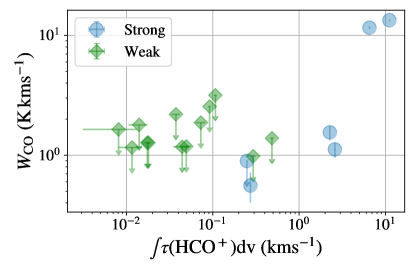
Figure 6: The integrated CO intensity ($W_{\rm{CO}}=\int T_{b}dv$) versus the integrated HCO⁺ optical depth for velocity ranges with strong, narrow absorption (blue circles) and weak, broad absorption (green diamonds) outlined in Figure 4. The CO spectra are from Dame et al. (in preparation). Upper limits are indicated with downward arrows.

5 Comparison to atomic gas properties

To investigate the connection between atomic gas properties and molecule formation, we compare the Gaussian-fitted components in the H I absorption spectra to those in the molecular absorption spectra (see Figure 2). For each molecular absorption feature, we find the H I absorption feature closest in velocity space and assume that they are associated with the same interstellar absorbing structure. We make exceptions for low latitude sources, where velocity crowding introduces significant ambiguity. In these cases, if two H I absorption features are within 1 $\,{\rm km\,s^{-1}}$ but one is a broad, weak feature ($\Delta v>10$ $\,{\rm km\,s^{-1}}$, $\tau<0.1$), we take the narrower, stronger feature to be the most probable match, even if it is not the closest in velocity space. In cases where multiple molecular absorption features are matched to the same atomic absorption feature, we consider the sum of the column densities of all matched molecular components in the following analysis.

In Figure 7, we show the cumulative distribution functions (CDFs) of the spin temperature, optical depth, and turbulent Mach number of H I structures seen in absorption towards our background sources (all quantities were constrained by 21-SPONGE). The turbulent Mach number—the ratio of the three dimensional turbulent velocity to the sound speed—is given by

$$M_{t}=2.05\Bigg{(}\frac{21.866\Delta v_{{\rm H\,{\small I}}{}}^{2}}{T_{s}}-1\Bigg{)}^{1/2},$$ (6)

where $\Delta v_{{\rm H\,{\small I}}{}}$ is the FWHM of the Gaussian H I component. The black CDF is for all H I structures, while the blue, orange, green, and red CDFs are for the H I structures that also show HCO⁺, HCN, HNC, and C₂H absorption, respectively.

From these CDFs, it is immediately clear that H I structures with a molecular component have higher optical depths and lower spin temperatures (so lower kinetic temperatures) than the general population of cold H I structures in the directions of our background sources. In particular, whereas the total population of H I structures exhibits a large range in H I optical depths and spin temperatures, the H I structures with a molecular component all have optical depths $>0.1$ and spin temperatures $\lesssim 80$ K. There is not such a marked difference in the turbulent Mach number of the different distributions, but the turbulent Mach numbers do appear higher for structures with a molecular component, $M_{t}\gtrsim 2$. There is no apparent difference between different molecular species, but this analysis does not necessarily include the broad component HCO⁺ absorption that is not always fit in our Gaussian decomposition (Section 4.2). Moreover, our sample size is modest, and few structures do not show absorption from all four species.

Figure 7: CDFs of the H I optical depth (top), the H I spin temperature (middle) and the H I turbulent Mach number (bottom) measured by Murray et al. (2018) in the direction of the background sources in this work. The CDF for all components is shown in black. The CDFs for H I features associated with HCO⁺, HCN, HNC, and C₂H absorption are shown in blue, orange, green, respectively. Error estimates derived from bootstrapping are shown.

These results suggest that regions of the CNM with higher optical depths (more CNM increases the production of H₂ and other molecules) and lower temperatures (meaning more shielded against the ISRF) are more conducive to forming molecules. Such regions also tend to have a higher turbulent Mach number. However, in most cases the 1D turbulent velocities are not systematically higher for features with a molecular component, suggesting that the higher turbulent Mach number is largely a reflection of the lower $T_{s}$.

These results are also summarized in Figure 8, where we compare HCO⁺ column densities with H I optical depths and spin temperatures. Points are colored according to turbulent Mach number. HCO⁺ absorption detections are shown as stars, while $3\sigma$ upper limits for non-detections are shown as circles. We do not show here features for which 21-SPONGE was unable to determine the H I spin temperature. Again, we see that molecular gas is associated with H I that is colder, optically thicker, and has a higher turbulent Mach number than the mean of the H I cloud sample in this study. For all H I structures along these sightlines, the mean values $(\tau,T_{S},M_{t})$ are $(0.2,171~{}\rm{K},3.6)$, while for H I structures with a molecular component, the mean values are $(0.7,42~{}\rm{K},4.4)$.

Figure 8 also shows that many components with $T_{s}<80$ K, as well as many components with $\tau>0.1$, do not have detected molecular column densities. This means that low $T_{s}$ and high H I optical depth are necessary but not sufficient conditions for molecule production.

Previously, Godard et al. (2010) showed that it is hard to reproduce HCO⁺ column densities larger than few $\times 10^{12}$ $\,{\rm cm^{-2}}$ in the diffuse ISM with PDR models. In Figure 8 we see several detections with such high column densities. We also see that these components have H I temperature in the range 40–80 K (the peak of the CNM distribution was found to be around 50–60 K; Heiles & Troland, 2003; Murray et al., 2018), peak H I optical depth $\sim 1$, and $M_{t}>3$ (colors indicate turbulent Mach number). These four detections also have higher 1D turbulent velocities than detections that show only weak molecular absorption, $v_{t}\gtrsim 1$ $\,{\rm km\,s^{-1}}$ (see Figure 9, where points are colored according to the 1D turbulent velocity), suggesting that the higher turbulent Mach numbers are a product of both the colder temperatures and the turbulent velocities. We discuss these relatively warmer, more turbulent features further in Paper II.

Figure 8: The HCO⁺ column density versus the H I optical depth (top) and spin temperature (bottom) for Gaussian components identified in the H I and HCO⁺ absorption spectra. HCO⁺ detections are shown as filled stars. The $3\sigma$ upper limits for non-detections are shown as filled circles. All points are colored according to the H I turbulent Mach number, $M_{t}$. Structures for which 21-SPONGE could not determine the spin temperature are not included in these plots.

Figure 9: Same as Figure 8, but points are colored according to the 1D turbulent velocity, $v_{t}$, of the atomic gas structures.

6 Comparison of different molecular species

A comparison of different molecular species contains valuable information about formation and destruction processes. We therefore compare the column densities and absorption line properties of HCN, C₂H, HCO⁺, and HNC, and place our results in the context of previous studies.

6.1 Line of sight abundances

Table 7: Column density ratios for different sightlines observed in this work. Column 1: name of background radio continuum source; Column 2: ratio of HCN column density to HNC column density; Column 3: ratio of C₂H column density to HCO⁺ column density. A dagger ($\dagger$) indicates that one or both of the measured column densities is a lower limit.

The abundance of molecular species studied here is determined by the rates of formation and destruction processes and may depend on different interstellar environments. For example, in cold and dense interstellar clouds, where the gas is largely shielded from external ultraviolet radiation, the HNC/HCN abundance ratio is expected to be close to 1 based on equilibrium chemical models (Aguado et al., 2017). However, in regions illuminated by ultraviolet photons, HNC is photodissociated faster than HCN resulting in HCN being significantly more abundant than HNC. This could happen in both diffuse interstellar clouds (Liszt & Lucas, 2001; Godard et al., 2010) and in photon-dominated regions (Aguado et al., 2017). Similarly, considering that both HCO⁺ and C₂H are products of CH${}_{3}^{+}$, the abundances of these molecules are expected to be correlated, e.g. Godard et al. (2009).

For the four lines of sight where both HNC and HCN are detected (3C120, 3C123A, 3C154, and 3C454.3, excluding lower limits; see Table 6.1) we find $\langle N(\text{HNC}{})/N(\text{HCN}{})\rangle=0.20\pm 0.02$. Similarly, for the four lines of sight where both C₂H and HCO⁺ are detected (3C120, 3C123A, 3C154, and 3C454.3, excluding lower limits; see Table 6.1), we find $\langle N(\text{C\textsubscript{2}H}{})/N(\text{HCO\textsuperscript{+}}{})\rangle=13.3\pm 6.9$. This ratio decreases with increasing $N(\text{HCO\textsuperscript{+}}{})$ (see Section 6.2 for a further discussion of this observation). Our results are consistent with previous measurements from Liszt & Lucas (2001), who found $\langle N(\text{HNC}{})/N(\text{HCN}{})\rangle=0.21\pm 0.05$, and Lucas & Liszt (2000), who found $\langle N(\text{C\textsubscript{2}H}{})/N(\text{HCO\textsuperscript{+}}{})\rangle=14.5\pm 6.7$.

Our results for HCN and HNC are generally not consistent with predictions from PDR models from the literature. For example, (Aguado et al., 2017) used the Meudon PDR code (Le Petit et al., 2006) to model the chemistry of a typical diffuse cloud. They considered a plane-parallel cloud with a total visual extinction of $A_{V}=1$ mag illuminated at both sides by the ISRF of 1–3 Draine fields, and considered a range of densities of H nuclei of $10^{2}$–$10^{4}$ $\,{\rm cm^{-3}}$. They found $N(\text{HNC}{})/N(\text{HCN}{})\sim 0.5$–1. While these results are only slightly higher than the observed values, they propagate to CN/HCN ratios one or two orders of magnitude above the observed value.

6.2 Gaussian components

6.2.1 Column density ratios

We measure the column density of each Gaussian component, where $\int\tau dv=1.064\,\tau_{0}\,\Delta v_{0}$ for a Gaussian feature with peak optical depth $\tau_{0}$ and FWHM $\Delta v_{0}$. Figure 10 shows the distribution of these column densities. The slope of $N(\text{C\textsubscript{2}H}{})/N(\text{HCO\textsuperscript{+}}{})$ becomes shallower for $N(\text{HCO\textsuperscript{+}}{})\lesssim 10^{12}$ $\,{\rm cm^{-2}}$—this explains why $N(\text{C\textsubscript{2}H}{})/N(\text{HCO\textsuperscript{+}}{})$ decreases at high $N(\text{HCO\textsuperscript{+}}{})$. The HCN column density increases faster than linearly with the HCO⁺ column density. The HNC and HCN column densities scale linearly with each other.

We find $\langle N(\text{C\textsubscript{2}H}{})/N(\text{HCO\textsuperscript{+}}{})\rangle=18.8\pm 9.5$, $\langle N(\text{HCN}{})/N(\text{HCO\textsuperscript{+}}{})\rangle=1.7\pm 0.9$, and $\langle N(\text{HNC}{})/N(\text{HCN}{})\rangle=0.22\pm 0.07$ (or equivalently, $\langle N(\text{HCN}{})/N(\text{HNC}{})\rangle=4.9\pm 1.3$). These ratios are consistent with those measured along the total line of sight (Section 6.1), including the large dispersion in $N(\text{C\textsubscript{2}H}{})/N(\text{HCO\textsuperscript{+}}{})$ and $N(\text{HCN}{})/N(\text{HCO\textsuperscript{+}}{})$. Previously, Godard et al. (2010) found $\langle N(\text{HCN}{})/N(\text{HCO\textsuperscript{+}}{})\rangle=1.9\pm 0.9$ and $\langle N(\text{HCN}{})/N(\text{HNC}{})\rangle=4.8\pm 1.3$ at low Galactic latitudes ($|b|<1$), and Liszt & Lucas (2001) found $\langle N(\text{HNC}{})/N(\text{HCN}{})\rangle=4.8\pm 1.1$ and $\langle N(\text{HCN}{})/N(\text{HCO\textsuperscript{+}}{})\rangle=1.47\pm 0.86$ at higher Galactic latitudes ($1.6<|b|<38.2$). Our results, measured in the direction of sources with latitudes $4.0<|b|<38.2$, are consistent with both of these previous works, although two of our sources were also included in Liszt & Lucas (2001).

The similarity in line ratios across Galactic latitude seen by Liszt & Lucas (2001), Godard et al. (2010), and this work suggest that gas in the Galactic plane is chemically similar to gas in the solar neighborhood. This trend was noticed by Godard et al. (2010), but the results here verify that this relationship persists to lower column densities (by a factor of a few) than probed by either of the previous experiments.

Figure 10: Comparisons of the C₂H column densities to the HCO⁺ column densities (top), the HCN column densities to the HCO⁺ column densities (middle), and the HNC column densities to the HCN column densities (bottom), for features identified in our Gaussian decomposition.

6.2.2 FWHM ratios

It has long been known that different molecular species in the diffuse ISM do not share the same kinematics. In particular, differences in the linewidths of absorption/emission features of different species have been suggested as evidence for the formation of these species under different environmental conditions. We compare the FWHMs between different species observed here in Figure 11. The mean ratio of the C₂H FWHMs to the HCO⁺ FWHMs is roughly $1.2:1$. The mean ratio of the HCN FWHMs to the HNC FWHMs is approximately $1:1$. The mean ratio of the HCN FWHMs to the HCO⁺ FWHMs and the mean ratio of the HNC FWHMs to the HCO⁺ FWHMs are both roughly $0.9:1$. Our measurement of the relative narrowness of HCN and HNC with respect to HCO⁺ is consistent with Godard et al. (2010), whose data set also included measurements from Lucas & Liszt (1996) and Liszt & Lucas (2001). We note, though, that there is considerable scatter in Figure 11 and that these measured ratios have uncertainties of $\sim 0.3$, meaning that our estimates for the line ratios are also not statistically significantly different from $1:1$.

Liszt & Lucas (2001) and Godard et al. (2010) previously observed that absorption by CN-bearing molecules is narrower than absorption by HCO⁺ at mm wavelengths, while Lambert et al. (1990) showed that CN absorption is systematically narrower than CH⁺ absorption at optical wavelengths. Liszt et al. (2019) also found that CO absorption is narrower than HCO⁺ absorption at mm wavelengths. Molecular absorption lines are turbulently broadened, so it has been suggested that HCO⁺ and CH⁺ lines are broader because these species are formed preferentially in turbulent, dynamic environments like TDRs and shocks (Godard et al., 2010; Liszt et al., 2019). Crane et al. (1995) and Pan et al. (2005) suggested that the differences in linewidths indicated that species like HCO⁺ and CH⁺ trace more diffuse regions such as cloud envelopes, while species like CN and HCN trace denser regions or molecular clouds. Liszt & Lucas (2001) also note that the molecular absorption linewidths may be produced by the turbulence of many structures along the line of sight rather than a single “cloud.” We detect HCO⁺ linewidths that are marginally broader than HCN or HNC linewidths, consistent with the idea that HCO⁺ forms in more turbulent environments than CN bearing species. Nevertheless, a larger data set is needed to place tighter statistical constraints on the relative widths of different species.

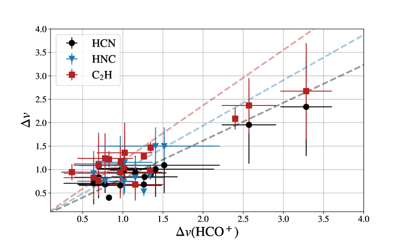
Figure 11: A comparison of the FWHMs of Gaussian fitted functions (Tables 9, 9, 9, 9). HCO⁺ FWHMs are shown on the $x$-axis. The $y$-axis displays the FWHMs for HCN (black circles), HNC (blue triangles), and C₂H (red squares).

7 Temporal stability of line profiles

Temporal variations in absorption line profiles against background radio continuum sources have long been used as a probe for small (AU) scale structure in the ISM (Stanimirović & Zweibel, 2018, and references therein). Such variability has been observed in H I (e.g., Crovisier et al., 1985; Greisen & Liszt, 1986; Diamond et al., 1989; Faison & Goss, 2001; Brogan et al., 2005; Roy et al., 2012) and several molecular lines (Marscher et al., 1993; Moore & Marscher, 1995), although the interpretation of the observed variations has been controversial (Thoraval et al., 1996; Heiles, 1997; Deshpande, 2000). The observed AU-scale structure in H I often has densities high enough for the existence of various molecular species. Detecting variability in molecular spectral lines therefore offers an exciting way of probing internal structure of over-dense H I structures.

In Table 8, we compare the integrated optical depths for HCN, C₂H (considering only the two transitions listed in Table 1), HCO⁺, and HNC measured in this work to those measured in previous surveys (Lucas & Liszt, 1996, 2000; Liszt & Lucas, 2001). Observations from these previous works were obtained between 1993 and 1997 with different antenna and receiver setups from those used here and reduced using different software. Our observations were obtained between 2018 and 2020, meaning that we are probing optical depth changes over a span of $\sim 25$ years in Table 8. We find only modest changes in the integrated optical depths, $<3.5\sigma$ differences in all cases. Two cases with over 3$\sigma$ significance are both in the case of 3C111 (HNC and C₂H) and probe variability on time scales of 25 years. 3C111 is especially interesting as Rybarczyk et al. (2020) found significant spatial variations in the H I optical depths between the different components of this source.

Figure 12 further shows the optical depth spectra of HCO⁺ in the direction of 3C120 and 3C454.3 measured here and those measured by Luo et al. (2020). Both were obtained with ALMA using similar spectral setups; the ALMA-SPONGE spectra were obtained in 2018, while the Luo et al. (2020) spectra were obtained in 2015, so these sightlines probe optical depth changes of $\sim 3$ years. The HCO⁺ optical depth spectra show no significant change with respect to the Luo et al. (2020) data taken 3 years earlier—the peak optical depths differ by $0.001$–$0.002$, a $<1\%$ difference detected at $<1\sigma$.

Our sample of sightlines with multi-epoch measurements is limited to five, two of which are non-detections. For these sightlines, the lack of short-term variations in the absorption profiles suggests that the molecular component of the gas is not highly structured on scales $\lesssim 100$ AU in these directions. This is consistent with previous observations that molecular absorption line profiles are generally stable over time. Liszt & Lucas (2000) found that HCO⁺ and OH absorption line profiles were generally stable over 3–5 year intervals in the direction of multiple background sources. Wiklind & Combes (1997) showed that HCO⁺ absorption spectra in the direction of Centaurus A were stable over a roughly 7 year span, and Han et al. (2017) showed that HCO⁺ absorption spectra in the direction of BL Lac and NRAO 150 were stable over $\sim$20 years. Furthermore, Liszt & Lucas (2000) argued that the modest changes detected in molecular absorption line profiles over time were most likely caused by small-scale changes in chemical abundances rather than by the presence of highly overdense, AU-scale structures.

Figure 12: The HCO⁺ optical spectra in the direction of 3C120 (top) and 3C454.3 (bottom). The spectra from Luo et al. (2020), obtained by ALMA in 2015, are shown in orange. The spectra from this work, obtained by ALMA in 2018, are shown in blue.

Table 8: The integrated optical depths of HCO⁺, HCN, HNC, and C₂H measured by previous surveys (Column 3) and measured in this work (Column 4). The time elapsed between surveys is listed in Column 5, and the change in integrated optical depth is listed in Column 6. Superscripts in Column 3 indicate references, as follows—1: Lucas & Liszt 1996; 2: Liszt & Lucas 2001; 3: Lucas & Liszt 2000a.

Source	Species	$(\int\tau dv)_{1}$	$(\int\tau dv)_{2}$	$\Delta t$	$\Delta(\int\tau dv)$
		$10^{12}$ $\,{\rm cm^{-2}}$	$10^{12}$ $\,{\rm cm^{-2}}$	yr	$10^{12}$ $\,{\rm cm^{-2}}$
3C111	HCO+	$13.32\pm 0.65^{1}$	$>11.054$	26
	HCN	$13.572\pm 0.276^{2}$	$>12.710$	25
	HNC	$3.149\pm 0.025^{2}$	$3.606\pm 0.129$	25	$0.457\pm 0.131$
	C2H	$1.913\pm 0.023^{3}$	$2.057\pm 0.033$	25	$0.144\pm 0.04$
3C273	HCO+	nd	nd	24
3C345	HCO+	nd	nd	24
3C454.3	HCO+	$0.32\pm 0.02^{1}$	$0.276\pm 0.004$	24	$0.044\pm 0.02$
	HCN	$0.120\pm 0.013^{2}$	$0.112\pm 0.004$	23	$0.008\pm 0.014$
	HNC	$0.046\pm 0.019^{2}$	$0.024\pm 0.002$	23	$0.022\pm 0.019$
	C2H	$0.152\pm 0.025^{3}$	$0.106\pm 0.004$	23	$0.046\pm 0.025$
BL Lac	HCO+	$2.30\pm 0.07^{1}$	$2.260\pm 0.004$	26	$0.04\pm 0.07$
	HCN	$2.360\pm 0.080^{2}$	$2.293\pm 0.002$	25	$0.067\pm 0.080$

8 Discussion

8.1 The atomic gas properties necessary for molecule formation

By comparing the Gaussian components identified in the 21-SPONGE H I absorption spectra (Murray et al., 2015, 2018) with the Gaussian components identified in the ALMA-SPONGE and NOEMA-SPONGE molecular absorption spectra, we have established H I optical depth, spin temperature, and turbulent Mach number thresholds for the formation of HCO⁺, HNC, HCN, and C₂H (Section 5). We find that molecular gas forms only if the H I optical depth of a gas structure exceeds $0.1$, the spin temperature—approximately equal to the kinetic temperature—is less than 80 K, and the turbulent Mach number is greater than $\sim 2$. In our sample, these conditions appear necessary but not sufficient for the formation of HCO⁺, C₂H, HCN, and HNC, as several H I absorption features satisfy these criteria but do not have a molecular component. We do not find significantly different thresholds for the different species, although our sample size is modest.

The optical depth threshold of 0.1 is similar to that established by Despois & Baudry (1985) for CO formation at $|b|<2^{\circ}{}$. However, our $T_{s}$ threshold ($T_{s}\lesssim 80$ K) is significantly lower than theirs ($T_{s}\sim 100\text{--}350$ K). We note, though, that Despois & Baudry (1985) derived $T_{s}$ using an isothermal approximation of channels with CO emission which is known to result in higher spin temperatures relative to Gaussian decomposition (Murray et al., 2015). They also used CO emission observations at $\sim 4\arcmin{}.3$ beamwidth, which probe more gas than the H I pencil beam and are less sensitive to low and even moderate column density gas than CO absorption observations. Observations of 21 cm H I and mm wavelength molecular absorption in the same direction have been otherwise limited to a very small number of sightlines ($N=1$–3; Moore & Marscher, 1995; Liszt & Lucas, 2000, 2004; Liszt & Gerin, 2018). For example Liszt & Lucas (2000) established that strong HCO⁺ absorption was associated with lower $\langle T_{s}\rangle$, $46$–$103$ K, in three directions (see Section 4.2).

The CNM associated with molecule formation in the diffuse ISM is thus systematically colder and more optically thick than the mean of the total cold H I cloud population. CNM structures with a molecular component also have higher turbulent Mach numbers than the general H I cloud population, which is a reflection of the colder temperature in most cases, as the 1D turbulent velocities are not systematically higher than the general cloud population. It is also interesting to note that the H I temperature threshold we find for molecule formation, 80 K, is near the mean kinetic temperature estimated from FUV observations of H₂ ($55-80$ K; Savage et al., 1977; Rachford et al., 2002, 2009b). This temperature agreement is expected if H I and H₂ are co-spatial, as is the case for H₂ forming out of the CNM on the surface of dust grains and being injected back to the CNM. The high turbulent Mach numbers seen here in the direction of diffuse molecular gas is consistent with previous observations of cold H I in the direction of Perseus (e.g., Burkhart et al., 2015).

A relationship between the H I column density and H₂ formation has long been known. The H I-to-H₂ transition has been extensively studied in theory and using observations of both entire galaxies and individual molecular clouds. The total gas column density threshold for H₂ formation has been well established (e.g., Savage et al., 1977; Krumholz et al., 2009; Bellomi et al., 2020, and references therein), and many studies have also noticed a threshold for CO formation (e.g., Lombardi et al., 2006; Wong et al., 2009; Leroy et al., 2009; Lee et al., 2014; Imara & Burkhart, 2016) which is higher (Lee et al., 2014, $A_{V}\sim 1-2$, e.g.,) than that of H₂ ($A_{V}\sim 0.25$). Observationally established thresholds for the formation of other molecular species have been rare. Our results are consistent with the previous work of Lucas & Liszt (1996) and Lucas & Liszt (2000) for HCO⁺ and C₂H, although our observations are more sensitive than theirs by a factor of $2$–$3$. Both simulations from Gong et al. (2020) (we discuss this more in Paper II) and our ALMA/NOEMA observations show a transition from atomic to molecular gas at $N({\rm H\,{\small I}}{})\sim 5\times 10^{20}$ cm^-2. This threshold appears consistent with that of H₂ and somewhat lower than that of CO. This clearly demonstrates the importance of shielding in building molecular abundances.

8.2 The significance of the UNM in molecule formation

Murray et al. (2018) quantified the fraction of thermally unstable H I along each line of sight. Although we find that the UNM column density is not directly correlated with the total quantity of molecular gas, it is nevertheless clearly important in setting the HCO⁺ column densities. As we have shown in Figure 3, positions with the highest C₂H, HCO⁺, HCN, and HNC column densities also tend to have a significant quantity of UNM gas, $10^{20}$–$10^{21}$ $\,{\rm cm^{-2}}$, comprising $\sim 30$–$70\%$ of all atomic gas along those lines of sight. The UNM plays a role in shielding but also may reveal mixing of the CNM and WNM, which is suggested to enhance the abundances of certain molecular species, including HCO⁺ (Valdivia et al., 2016; Lesaffre et al., 2020).

Previous observational and theoretical work has highlighted the role of the multiphase atomic ISM in molecule formation. For example, Bialy et al. (2015) investigated the H I-to-H₂ transition in several regions in the Perseus molecular cloud, where Lee et al. (2012) have found a well-defined threshold for H₂ formation, $(8\text{--}14)\times 10^{20}$ $\,{\rm cm^{-2}}$. By fitting the Sternberg et al. (2014) model for H₂ formation in equilibrium and assuming that H I gas is multiphase and in pressure equilibrium, they constrained the volume density of H I in the atomic shielding envelope of Perseus. As the estimated densities were in the range $\sim 2-10$ cm^-3, they concluded that much of this H I is thermally unstable, possibly in a cooling transition from the WNM to CNM phases. The behavior in Perseus suggests that in addition to CNM, less dense UNM and perhaps some diffuse WNM, are important in controlling the H I-to-H₂ transition. Our observations indicate that the UNM is important for enhancing the abundances of species other than H₂ and CO, as well.

8.3 Interpretation of broad, faint HCO⁺ absorption

In a majority of sightlines, we find a broad, faint component to the HCO⁺ absorption that spans a large portion of the velocity space where H I absorption is observed (Section 4.2). Our study suggests that this broad HCO⁺ component is likely to be frequently seen in high-sensitivity observations. The H I coincident with this broad HCO⁺ absorption component has higher $\langle T_{S}\rangle$ than the H I at velocities where strong, narrow HCO⁺ absorption is observed, indicating that the fraction of H I in the CNM is lower at these velocities (e.g., Kim et al., 2014). If we assume that $N(\text{HCO\textsuperscript{+}}{})/N(\text{H\textsubscript{2}}{})$ is constant (Liszt & Lucas, 2000; Liszt et al., 2018), then we also find that the fraction of hydrogen in its molecular form is lower for velocities with broad absorption ($f_{\mathrm{mol}}\lesssim 0.1$, versus $f_{\mathrm{mol}}\gtrsim 0.2$ at velocities with a strong, narrow absorption component).

The fact that the broad component of HCO⁺ absorption is associated with gas that has a lower CNM fraction and a lower molecular fraction may indicate that it is probing the outer layers of molecular structures, where the turbulent mixing between the CNM and WNM allows for the formation of CH⁺ and HCO⁺. This would explain why the broad HCO⁺ absorption spans roughly the same velocity range as the cold H I observed by 21-SPONGE in nearly all sightlines (Figure 4). The relatively broad linewidths of the faint component of HCO⁺ absorption may also suggest formation in warmer, more diffuse interstellar environments (Falgarone et al., 2006). For example, Valdivia et al. (2017) and Lesaffre et al. (2020) showed that CH⁺—which contributes to the formation of HCO⁺—is formed efficiently in turbulent dissipation regions, at the edge of molecular clumps, and in slow shocks, where the H I is thermally unstable and the H₂ formation is out of equilibrium. In the Valdivia et al. (2017) simulations, most of the CH⁺ is produced in regions with H₂ fractions $\sim 0.003$–$0.3$ and with gas temperatures as high as $\sim 10^{2-3}$ K. Given the role CH⁺ plays in HCO⁺ formation, the broad HCO⁺ may trace the active regions of CH⁺ production.

We see no CO emission at velocities where the broad, faint HCO⁺ absorption is detected, although the resolution and sensitivity of CO emission observations from Dame et al. (2001) do not match those of our ALMA/NOEMA absorption spectra. Moreover, due to low excitation temperature, CO may not be detectable in emission (e.g., Lucas & Liszt, 1996; Liszt & Lucas, 2000). The possibility that the broad HCO⁺ absorption component is CO dark warrants further investigation, as it may contribute to the explanation of why HCO⁺ is a better tracer of the total gas content than CO in the diffuse ISM (Liszt et al., 2018). Liszt et al. (2019) have already shown that HCO⁺ linewidths are broader than CO linewidths, which is consistent with the idea that HCO⁺ is enhanced in diffuse, turbulent regions of the ISM relative to CO. Moreover, Figure 1 of Luo et al. (2020) suggests that there is indeed broad, faint HCO⁺ absorption in the direction of 3C454.3—only marginally detected in our less sensitive spectra—that is predominately CO dark. However, a quantitative comparison of the amount of HCO⁺ occupied by this broad component with the total amount of CO dark molecular gas has not yet been made.

8.4 The similarity of gas at different latitudes

We show that the relative abundances of different species are similar between this study and several previous surveys, even though these measurements collectively span Galactic latitudes between $<1^{\circ}$ and $\sim 40^{\circ}$ (Table 6.1; Liszt & Lucas, 2001; Godard et al., 2010). Similarly, we do not find significant differences between the FWHM ratios of different species with those measured in previous experiments over the same range of latitudes (Godard et al., 2010), although these ratios are less tightly constrained.

The similarity in the relative abundances and linewidths of different species suggests that similar chemical pathways operate across the Galaxy, both in the plane and in the solar neighborhood. This is consistent with the interpretation of Godard et al. (2010), but we have added significantly to the total sample of observations of diffuse molecular gas, including gas at column densities lower than those probed by Liszt & Lucas (2001) and Godard et al. (2010) by a factor of a few. Godard et al. (2010) suggested that the lack of dependence on Galactic latitude indicated that the formation mechanism of different species was weakly dependent on the ambient UV field, perhaps pointing to a ubiquitous mechanism like turbulent dissipation. As discussed further in Paper II, it will be important to observe tracers of non-equilibrium processes like CH⁺ or SiO and test PDR predictions to verify this hypothesis.

8.5 Is there a molecular component to tiny scale atomic structure?

In Section 7, we show that over periods of 3–25 years, HCO⁺, C₂H, HCN, and HNC absorption spectra are generally stable for our small sample of sightlines with multi-epoch absorption observations.

Marscher et al. (1993) and Moore & Marscher (1995) detected temporal variations in the H₂CO optical depth in the direction of 3C111, arguing in favor of dense clouds ($n\sim 10^{6}$ $\,{\rm cm^{-3}}$) in this direction at a scale of $\sim 10$–$100$ AU. However, Thoraval et al. (1996) showed that the H₂CO optical depth variations were most probably a result of changes in the relative abundance or excitation of H₂CO rather than tiny dense structures. We find marginal variations ($3.5\sigma$) in the integrated optical depths of HNC, and C₂H in the direction of 3C111 (Section 7), which suggests that there are not extremely dense structures on scales of $\sim 10$ AU in this direction as suggested by Marscher et al. (1993) and Moore & Marscher (1995), consistent with the interpretation of Thoraval et al. (1996).

No other sources show temporal variations in the HCO⁺, HCN, HNC, or C₂H optical depths at a level of $>2.2\sigma$. BL Lac—in the direction of the Lacerta molecular cloud—shows remarkably stable absorption spectra, $<1\sigma$ changes over $\sim 25$ years (Lucas & Liszt, 1996; Liszt & Lucas, 2001). Han et al. (2017) previously found no difference in HCO⁺ absorption spectra obtained with the Korean VLBI Network to the HCO⁺ absorption spectra from Lucas & Liszt (1996) 20 years earlier in the direction of BL Lac. Similarly, the integrated and peak optical depths measured here in the direction of 3C120 and 3C454.3 show $<1\sigma$ changes compared to those obtained by Luo et al. (2020) 3 years earlier.

Spatial variations in the H I optical depths toward the multiple-component sources 3C111 and 3C123 have revealed TSAS at a scale of $\sim 10^{4}$. 3C111 is a particularly intriguing case, as Dickey & Terzian (1978), Greisen & Liszt (1986), Goss et al. (2008), and Rybarczyk et al. (2020) have all measured optical depth variations of $\sim 0.3$–0.4 between its different components, corresponding to column density changes of $\gtrsim 10^{20}$ $\,{\rm cm^{-2}}$ at scales of $\sim 10^{4}$ AU. Goss et al. (2008) and Rybarczyk et al. (2020) also previously found H I optical depth variations at a level of $\sim 0.1$ toward the different components of 3C123. Unfortunately, due to a combination of poor sensitivity toward the fainter components and line saturation, we can only put very weak upper limits on the spatial molecular optical depth variations in these directions. Future sensitive observations of unsaturated molecular absorption lines are required to test if the these lines vary with the H I on scales of $10^{4}$ AU.

We note that the H I optical depth in the direction of 3C138 has been observed to vary dramatically, both spatially ($\sim$few$\times 10$ AU) and temporally ($\lesssim 7$ yr), making it a regular subject of TSAS investigations. Diamond et al. (1989) and Davis et al. (1996) both found spatial variations in the H I optical depth measured across resolved images of 3C138 obtained using very long baseline interferometry (VLBI) techniques. Later, Faison & Goss (2001), Brogan et al. (2005), and Roy et al. (2012) constructed H I optical depth maps against 3C138 using the Very Long Baseline Array (VLBA) across three different epochs. They detected milliarcsecond H I optical depth variations (corresponding to spatial scales of $\sim 25$ AU) in each epoch, as well as significant variations across epochs. These measurements have been attributed to H I structures with densities $\sim 10^{4}$ $\,{\rm cm^{-3}}$. Moreover, Deshpande et al. (2000), who were critical of the interpretation of optical depth variations as evidence of dense structures, acknowledged that the optical depth variations in the direction of 3C138 cannot be explained by geometrical effects and are likely due to true tiny, dense structures. We see no HCO⁺, C₂H, HCN, or HNC absorption in the direction of 3C138. The full sky maps in Pelgrims et al. (2020), made from the Lallement et al. (2019) 3D dust maps, suggest that this line of sight intersects the Local Bubble wall at $\lesssim 150$ pc, while the H I associated with Taurus lies at a distance of $\lesssim 140$ pc (Schlafly et al., 2014). Considering that the absorbing gas is located inside the Local Bubble wall (e.g., Lallement et al., 2014), the lack of molecules associated with TSAS in this direction could be caused by the physical conditions associated with Local Bubble (e.g., Stanimirović et al., 2010).

9 Conclusion

We have complemented H I observations (VLA; Murray et al., 2018) with new HCO⁺, HCN, HNC, and C₂H (ALMA, NOEMA) observations in the direction of 20 background radio continuum sources with $4^{\circ}\leq|b|\leq 81^{\circ}$ to constrain the atomic gas conditions that are suitable for the formation of diffuse molecular gas. In our sample, we find that these molecular species form along sightlines where $A_{V}\gtrsim 0.25$, corresponding to $N_{\mathrm{H}}\gtrsim 5\times 10^{20}$ $\,{\rm cm^{-2}}$ (e.g., Zhu et al., 2017), consistent with a threshold for the H I-to-H₂ transition at solar metallicity (Savage et al., 1977). This confirms the trend noticed by Lucas & Liszt (1996) and Lucas & Liszt (2000) for HCO⁺ and C₂H, with absorption spectra $\sim 2$–$3$ times more sensitive than theirs. Moreover, we find that molecular gas is associated only with structures that have an H I optical depth $>0.1$, a spin temperature $<80$ K, and a turbulent Mach number $\gtrsim 2$.

We identify a broad, faint component to the HCO⁺ absorption in a majority of sightlines. In several cases this component spans nearly the entire range of velocities where H I is seen in absorption. The H I at velocities where only the faint, broad HCO⁺ absorption is observed has systematically higher $\langle T_{s}\rangle$ than the H I at velocities where strong, narrow HCO⁺ absorption is observed, indicating that the H I at these velocities has a lower CNM fraction (Kim et al., 2014). We also do not detect CO emission at these velocities, whereas CO emission is detected at nearly all velocities where strong HCO⁺ absorption is observed. The broad HCO⁺ may therefore be a good tracer of the CO dark molecular gas and deserves further investigation.

The relative column densities and linewidths of the different molecular species observed here are similar to those observed in previous experiments over a range of Galactic latitudes, suggesting that gas in the solar neighborhood and gas in the Galactic plane are chemically similar. For a select sample of previously-observed sightlines, we show that the absorption line profiles of HCO⁺, HCN, HNC, and C₂H are stable over periods of $\sim 3$ years and $\sim 25$ years, likely indicating that molecular gas structures in these directions are at least $\gtrsim 100$ AU in size.

In Paper II, we compare the observational results presented here to predictions from the PDR chemical model in Gong et al. (2017) and the ISM simulations in Gong et al. (2020) to investigate in detail the local physical conditions (density, radiation field, cosmic ray ionization rate) needed to explain the observed column densities.

Table 3: Gaussian fits to the C₂H absorption spectra. Column 1: Source name; Column 2: peak optical depth, $\tau_{0}$; Column 3: FWHM, $\Delta v_{0}$; Column 4: central velocity, $v_{0}$; Column 5: integrated optical depth. .

Table 4: Gaussian fits to the HCN absorption spectra. Column 1: Source name; Column 2: peak optical depth, $\tau_{0}$; Column 3: FWHM, $\Delta v_{0}$; Column 4: central velocity, $v_{0}$; Column 5: integrated optical depth. Components for sightlines with saturated absorption are superscripted by a dagger ($\dagger$).

Table 5: Gaussian fits to the HCO⁺ absorption spectra. Column 1: Source name; Column 2: peak optical depth, $\tau_{0}$; Column 3: FWHM, $\Delta v_{0}$; Column 4: central velocity, $v_{0}$; Column 5: integrated optical depth. Components for sightlines with saturated absorption are superscripted by a dagger ($\dagger$).

Table 6: Gaussian fits to the HNC absorption spectra. Column 1: Source name; Column 2: peak optical depth, $\tau_{0}$; Column 3: FWHM, $\Delta v_{0}$; Column 4: central velocity, $v_{0}$; Column 5: integrated optical depth. Components for sightlines with saturated absorption are superscripted by a dagger ($\dagger$).

References

- Aguado et al. (2017) Aguado, A., Roncero, O., Zanchet, A., Agúndez, M., & Cernicharo, J. 2017, ApJ, 838, 33, doi: 10.3847/1538-4357/aa63ee
- Astropy Collaboration et al. (2013) Astropy Collaboration, Robitaille, T. P., Tollerud, E. J., et al. 2013, A&A, 558, A33, doi: 10.1051/0004-6361/201322068
- Astropy Collaboration et al. (2018) Astropy Collaboration, Price-Whelan, A. M., Sipőcz, B. M., et al. 2018, AJ, 156, 123, doi: 10.3847/1538-3881/aabc4f
- Bellomi et al. (2020) Bellomi, E., Godard, B., Hennebelle, P., et al. 2020, arXiv e-prints, arXiv:2009.05466. https://arxiv.org/abs/2009.05466
- Bialy et al. (2017) Bialy, S., Burkhart, B., & Sternberg, A. 2017, ApJ, 843, 92, doi: 10.3847/1538-4357/aa7854
- Bialy et al. (2015) Bialy, S., Sternberg, A., Lee, M.-Y., Le Petit, F., & Roueff, E. 2015, ApJ, 809, 122, doi: 10.1088/0004-637X/809/2/122
- Bohlin et al. (1978) Bohlin, R. C., Savage, B. D., & Drake, J. F. 1978, ApJ, 224, 132, doi: 10.1086/156357
- Bolatto et al. (2011) Bolatto, A. D., Leroy, A. K., Jameson, K., et al. 2011, ApJ, 741, 12, doi: 10.1088/0004-637X/741/1/12
- Brogan et al. (2005) Brogan, C. L., Zauderer, B. A., Lazio, T. J., et al. 2005, AJ, 130, 698, doi: 10.1086/431736
- Burkhart et al. (2015) Burkhart, B., Lee, M.-Y., Murray, C. E., & Stanimirović, S. 2015, ApJ, 811, L28, doi: 10.1088/2041-8205/811/2/L28
- Crane et al. (1995) Crane, P., Lambert, D. L., & Sheffer, Y. 1995, ApJS, 99, 107, doi: 10.1086/192180
- Crovisier (1978) Crovisier, J. 1978, A&A, 70, 43
- Crovisier et al. (1985) Crovisier, J., Dickey, J. M., & Kazes, I. 1985, A&A, 146, 223
- Dame et al. (2001) Dame, T. M., Hartmann, D., & Thaddeus, P. 2001, ApJ, 547, 792, doi: 10.1086/318388
- Davis et al. (1996) Davis, R. J., Diamond, P. J., & Goss, W. M. 1996, MNRAS, 283, 1105, doi: 10.1093/mnras/283.4.1105
- Deshpande (2000) Deshpande, A. A. 2000, MNRAS, 317, 199, doi: 10.1046/j.1365-8711.2000.03631.x
- Deshpande et al. (2000) Deshpande, A. A., Dwarakanath, K. S., & Goss, W. M. 2000, ApJ, 543, 227, doi: 10.1086/317104
- Despois & Baudry (1985) Despois, D., & Baudry, A. 1985, A&A, 148, 83
- Diamond et al. (1989) Diamond, P. J., Goss, W. M., Romney, J. D., et al. 1989, ApJ, 347, 302, doi: 10.1086/168119
- Dickey & Terzian (1978) Dickey, J. M., & Terzian, Y. 1978, A&A, 70, 415
- Draine (1978) Draine, B. T. 1978, ApJS, 36, 595, doi: 10.1086/190513
- Endres et al. (2016) Endres, C. P., Schlemmer, S., Schilke, P., Stutzki, J., & Müller, H. S. P. 2016, Journal of Molecular Spectroscopy, 327, 95, doi: 10.1016/j.jms.2016.03.005
- Faison & Goss (2001) Faison, M. D., & Goss, W. M. 2001, AJ, 121, 2706, doi: 10.1086/320369
- Falgarone et al. (2006) Falgarone, E., Pineau Des Forêts, G., Hily-Blant, P., & Schilke, P. 2006, A&A, 452, 511, doi: 10.1051/0004-6361:20054087
- Field et al. (1969) Field, G. B., Goldsmith, D. W., & Habing, H. J. 1969, ApJ, 155, L149, doi: 10.1086/180324
- Gildas Team (2013) Gildas Team. 2013, GILDAS: Grenoble Image and Line Data Analysis Software. http://ascl.net/1305.010
- Glover & Clark (2012) Glover, S. C. O., & Clark, P. C. 2012, MNRAS, 421, 9, doi: 10.1111/j.1365-2966.2011.19648.x
- Godard et al. (2010) Godard, B., Falgarone, E., Gerin, M., Hily-Blant, P., & de Luca, M. 2010, A&A, 520, A20, doi: 10.1051/0004-6361/201014283
- Godard et al. (2009) Godard, B., Falgarone, E., & Pineau Des Forêts, G. 2009, A&A, 495, 847, doi: 10.1051/0004-6361:200810803
- Gong et al. (2018) Gong, M., Ostriker, E. C., & Kim, C.-G. 2018, ApJ, 858, 16, doi: 10.3847/1538-4357/aab9af
- Gong et al. (2020) Gong, M., Ostriker, E. C., Kim, C.-G., & Kim, J.-G. 2020, ApJ, 903, 142, doi: 10.3847/1538-4357/abbdab
- Gong et al. (2017) Gong, M., Ostriker, E. C., & Wolfire, M. G. 2017, ApJ, 843, 38, doi: 10.3847/1538-4357/aa7561
- Goss et al. (2008) Goss, W. M., Richards, A. M. S., Muxlow, T. W. B., & Thomasson, P. 2008, MNRAS, 388, 165, doi: 10.1111/j.1365-2966.2008.13300.x
- Green (2018) Green, G. 2018, The Journal of Open Source Software, 3, 695, doi: 10.21105/joss.00695
- Greisen & Liszt (1986) Greisen, E. W., & Liszt, H. S. 1986, ApJ, 303, 702, doi: 10.1086/164118
- Güver & Özel (2009) Güver, T., & Özel, F. 2009, MNRAS, 400, 2050, doi: 10.1111/j.1365-2966.2009.15598.x
- Han et al. (2017) Han, J., Yun, Y., & Park, Y.-S. 2017, Journal of Korean Astronomical Society, 50, 185, doi: 10.5303/JKAS.2017.50.6.185
- Heiles (1997) Heiles, C. 1997, ApJ, 481, 193, doi: 10.1086/304033
- Heiles & Troland (2003) Heiles, C., & Troland, T. H. 2003, ApJ, 586, 1067, doi: 10.1086/367828
- Heitsch et al. (2006) Heitsch, F., Slyz, A. D., Devriendt, J. E. G., Hartmann, L. W., & Burkert, A. 2006, ApJ, 648, 1052, doi: 10.1086/505931
- Hennebelle & Audit (2007) Hennebelle, P., & Audit, E. 2007, A&A, 465, 431, doi: 10.1051/0004-6361:20066139
- Hennebelle & Inutsuka (2006) Hennebelle, P., & Inutsuka, S.-i. 2006, ApJ, 647, 404, doi: 10.1086/505316
- Imara & Burkhart (2016) Imara, N., & Burkhart, B. 2016, ApJ, 829, 102, doi: 10.3847/0004-637X/829/2/102
- Inoue & Inutsuka (2012) Inoue, T., & Inutsuka, S.-i. 2012, ApJ, 759, 35, doi: 10.1088/0004-637X/759/1/35
- Inutsuka et al. (2015) Inutsuka, S.-i., Inoue, T., Iwasaki, K., & Hosokawa, T. 2015, A&A, 580, A49, doi: 10.1051/0004-6361/201425584
- Jenkins & Savage (1974) Jenkins, E. B., & Savage, B. D. 1974, ApJ, 187, 243, doi: 10.1086/152620
- Jones et al. (2001) Jones, E., Oliphant, T., & Peterson, P. 2001
- Kim et al. (2014) Kim, C.-G., Ostriker, E. C., & Kim, W.-T. 2014, ApJ, 786, 64, doi: 10.1088/0004-637X/786/1/64
- Koyama & Inutsuka (2002) Koyama, H., & Inutsuka, S.-i. 2002, ApJ, 564, L97, doi: 10.1086/338978
- Krumholz et al. (2009) Krumholz, M. R., McKee, C. F., & Tumlinson, J. 2009, ApJ, 693, 216, doi: 10.1088/0004-637X/693/1/216
- Lallement et al. (2019) Lallement, R., Babusiaux, C., Vergely, J. L., et al. 2019, A&A, 625, A135, doi: 10.1051/0004-6361/201834695
- Lallement et al. (2014) Lallement, R., Vergely, J. L., Valette, B., et al. 2014, A&A, 561, A91, doi: 10.1051/0004-6361/201322032
- Lambert et al. (1990) Lambert, D. L., Sheffer, Y., & Crane, P. 1990, ApJ, 359, L19, doi: 10.1086/185786
- Le Petit et al. (2006) Le Petit, F., Nehmé, C., Le Bourlot, J., & Roueff, E. 2006, ApJS, 164, 506, doi: 10.1086/503252
- Lee et al. (2014) Lee, M.-Y., Stanimirović, S., Wolfire, M. G., et al. 2014, ApJ, 784, 80, doi: 10.1088/0004-637X/784/1/80
- Lee et al. (2012) Lee, M.-Y., Stanimirović, S., Douglas, K. A., et al. 2012, ApJ, 748, 75, doi: 10.1088/0004-637X/748/2/75
- Lequeux (2005) Lequeux, J. 2005, The Interstellar Medium, doi: 10.1007/b137959
- Leroy et al. (2009) Leroy, A. K., Bolatto, A., Bot, C., et al. 2009, ApJ, 702, 352, doi: 10.1088/0004-637X/702/1/352
- Lesaffre et al. (2007) Lesaffre, P., Gerin, M., & Hennebelle, P. 2007, A&A, 469, 949, doi: 10.1051/0004-6361:20066807
- Lesaffre et al. (2020) Lesaffre, P., Todorov, P., Levrier, F., et al. 2020, MNRAS, 495, 816, doi: 10.1093/mnras/staa849
- Liszt & Gerin (2018) Liszt, H., & Gerin, M. 2018, A&A, 610, A49, doi: 10.1051/0004-6361/201731983
- Liszt et al. (2018) Liszt, H., Gerin, M., & Grenier, I. 2018, A&A, 617, A54, doi: 10.1051/0004-6361/201833167
- Liszt et al. (2019) —. 2019, A&A, 627, A95, doi: 10.1051/0004-6361/201935436
- Liszt & Lucas (2000) Liszt, H., & Lucas, R. 2000, A&A, 355, 333
- Liszt & Lucas (2001) —. 2001, A&A, 370, 576, doi: 10.1051/0004-6361:20010260
- Liszt & Lucas (2004) —. 2004, A&A, 428, 445, doi: 10.1051/0004-6361:20041650
- Liszt et al. (2010) Liszt, H. S., Pety, J., & Lucas, R. 2010, A&A, 518, A45, doi: 10.1051/0004-6361/201014510
- Lombardi et al. (2006) Lombardi, M., Alves, J., & Lada, C. J. 2006, A&A, 454, 781, doi: 10.1051/0004-6361:20042474
- Lucas & Liszt (1996) Lucas, R., & Liszt, H. 1996, A&A, 307, 237
- Lucas & Liszt (2000) Lucas, R., & Liszt, H. S. 2000, A&A, 358, 1069
- Luo et al. (2020) Luo, G., Li, D., Tang, N., et al. 2020, ApJ, 889, L4, doi: 10.3847/2041-8213/ab6337
- Marscher et al. (1993) Marscher, A. P., Moore, E. M., & Bania, T. M. 1993, ApJ, 419, L101, doi: 10.1086/187147
- McMullin et al. (2007) McMullin, J. P., Waters, B., Schiebel, D., Young, W., & Golap, K. 2007, in Astronomical Society of the Pacific Conference Series, Vol. 376, Astronomical Data Analysis Software and Systems XVI, ed. R. A. Shaw, F. Hill, & D. J. Bell, 127
- Moore & Marscher (1995) Moore, E. M., & Marscher, A. P. 1995, ApJ, 452, 671, doi: 10.1086/176338
- Müller et al. (2001) Müller, H. S. P., Thorwirth, S., Roth, D. A., & Winnewisser, G. 2001, A&A, 370, L49, doi: 10.1051/0004-6361:20010367
- Murray et al. (2018) Murray, C. E., Stanimirović, S., Goss, W. M., et al. 2018, ApJS, 238, 14, doi: 10.3847/1538-4365/aad81a
- Murray et al. (2015) —. 2015, ApJ, 804, 89, doi: 10.1088/0004-637X/804/2/89
- Nguyen et al. (2019) Nguyen, H., Dawson, J. R., Lee, M.-Y., et al. 2019, ApJ, 880, 141, doi: 10.3847/1538-4357/ab2b9f
- Pan et al. (2005) Pan, K., Federman, S. R., Sheffer, Y., & Andersson, B. G. 2005, ApJ, 633, 986, doi: 10.1086/491466
- Pelgrims et al. (2020) Pelgrims, V., Ferrière, K., Boulanger, F., Lallement, R., & Montier, L. 2020, A&A, 636, A17, doi: 10.1051/0004-6361/201937157
- Pety (2005) Pety, J. 2005, in SF2A-2005: Semaine de l’Astrophysique Francaise, ed. F. Casoli, T. Contini, J. M. Hameury, & L. Pagani, 721
- Pikel’Ner (1968) Pikel’Ner, S. B. 1968, Soviet Ast., 11, 737
- Planck Collaboration et al. (2014a) Planck Collaboration, Abergel, A., Ade, P. A. R., et al. 2014a, A&A, 571, A11, doi: 10.1051/0004-6361/201323195
- Planck Collaboration et al. (2014b) Planck Collaboration, Ade, P. A. R., Aghanim, N., et al. 2014b, A&A, 571, A13, doi: 10.1051/0004-6361/201321553
- Planck Collaboration et al. (2016) Planck Collaboration, Aghanim, N., Ashdown, M., et al. 2016, A&A, 596, A109, doi: 10.1051/0004-6361/201629022
- Rachford et al. (2002) Rachford, B. L., Snow, T. P., Tumlinson, J., et al. 2002, ApJ, 577, 221, doi: 10.1086/342146
- Rachford et al. (2009a) Rachford, B. L., Snow, T. P., Destree, J. D., et al. 2009a, ApJS, 180, 125, doi: 10.1088/0067-0049/180/1/125
- Rachford et al. (2009b) —. 2009b, ApJS, 180, 125, doi: 10.1088/0067-0049/180/1/125
- Roy et al. (2012) Roy, N., Minter, A. H., Goss, W. M., Brogan, C. L., & Lazio, T. J. W. 2012, ApJ, 749, 144, doi: 10.1088/0004-637X/749/2/144
- Rybarczyk et al. (2020) Rybarczyk, D. R., Stanimirović, S., Zweibel, E. G., et al. 2020, ApJ, 893, 152, doi: 10.3847/1538-4357/ab83f7
- Savage et al. (1977) Savage, B. D., Bohlin, R. C., Drake, J. F., & Budich, W. 1977, ApJ, 216, 291, doi: 10.1086/155471
- Schlafly et al. (2014) Schlafly, E. F., Green, G., Finkbeiner, D. P., et al. 2014, ApJ, 786, 29, doi: 10.1088/0004-637X/786/1/29
- Schöier et al. (2010) Schöier, F., van der Tak, F., van Dishoeck, E., & Black, J. 2010, LAMDA: Leiden Atomic and Molecular Database. http://ascl.net/1010.077
- Spitzer et al. (1973) Spitzer, L., Drake, J. F., Jenkins, E. B., et al. 1973, ApJ, 181, L116, doi: 10.1086/181197
- Stanimirović et al. (2014) Stanimirović, S., Murray, C. E., Lee, M.-Y., Heiles, C., & Miller, J. 2014, ApJ, 793, 132, doi: 10.1088/0004-637X/793/2/132
- Stanimirović et al. (2010) Stanimirović, S., Weisberg, J. M., Pei, Z., Tuttle, K., & Green, J. T. 2010, ApJ, 720, 415, doi: 10.1088/0004-637X/720/1/415
- Stanimirović & Zweibel (2018) Stanimirović, S., & Zweibel, E. G. 2018, ARA&A, 56, 489, doi: 10.1146/annurev-astro-081817-051810
- Sternberg et al. (2014) Sternberg, A., Le Petit, F., Roueff, E., & Le Bourlot, J. 2014, ApJ, 790, 10, doi: 10.1088/0004-637X/790/1/10
- Thoraval et al. (1996) Thoraval, S., Boisse, P., & Stark, R. 1996, A&A, 312, 973
- Valdivia et al. (2017) Valdivia, V., Godard, B., Hennebelle, P., et al. 2017, A&A, 600, A114, doi: 10.1051/0004-6361/201629905
- Valdivia et al. (2016) Valdivia, V., Hennebelle, P., Gérin, M., & Lesaffre, P. 2016, A&A, 587, A76, doi: 10.1051/0004-6361/201527325
- Virtanen et al. (2020) Virtanen, P., Gommers, R., Oliphant, T. E., et al. 2020, Nature Methods, 17, 261, doi: 10.1038/s41592-019-0686-2
- Wiklind & Combes (1997) Wiklind, T., & Combes, F. 1997, A&A, 324, 51. https://arxiv.org/abs/astro-ph/9701081
- Wolfire et al. (2003) Wolfire, M. G., McKee, C. F., Hollenbach, D., & Tielens, A. G. G. M. 2003, ApJ, 587, 278, doi: 10.1086/368016
- Wong et al. (2009) Wong, T., Hughes, A., Fukui, Y., et al. 2009, ApJ, 696, 370, doi: 10.1088/0004-637X/696/1/370
- Zhu et al. (2017) Zhu, H., Tian, W., Li, A., & Zhang, M. 2017, MNRAS, 471, 3494, doi: 10.1093/mnras/stx1580