Molecules with ALMA at Planet-forming Scales (MAPS) IV: Emission Surfaces and Vertical Distribution of Molecules

Abstract

The Molecules with ALMA at Planet-forming Scales (MAPS) Large Program provides a unique opportunity to study the vertical distribution of gas, chemistry, and temperature in the protoplanetary disks around IM Lup, GM Aur, AS 209, HD 163296, and MWC 480. By using the asymmetry of molecular line emission relative to the disk major axis, we infer the emission height ($z$) above the midplane as a function of radius ($r$). Using this method, we measure emitting surfaces for a suite of CO isotopologues, HCN, and C₂H. We find that ¹²CO emission traces the most elevated regions with $z/r>0.3$, while emission from the less abundant ¹³CO and C¹⁸O probes deeper into the disk at altitudes of $z/r~{}\lesssim~{}0.2$. C₂H and HCN have lower opacities and SNRs, making surface fitting more difficult, and could only be reliably constrained in AS 209, HD 163296, and MWC 480, with $z/r~{}\lesssim~{}0.1$, i.e., relatively close to the planet-forming midplanes. We determine peak brightness temperatures of the optically thick CO isotopologues and use these to trace 2D disk temperature structures. Several CO temperature profiles and emission surfaces show dips in temperature or vertical height, some of which are associated with gaps and rings in line and/or continuum emission. These substructures may be due to local changes in CO column density, gas surface density, or gas temperatures, and detailed thermo-chemical models are necessary to better constrain their origins and relate the chemical compositions of elevated disk layers with those of planet-forming material in disk midplanes. This paper is part of the MAPS special issue of the Astrophysical Journal Supplement.

1 Introduction

Protoplanetary disks are highly stratified in their physical and chemical properties (Williams & Cieza, 2011) with flared emitting surfaces set by the balance of hydrostatic equilibrium, as first recognized in their spectral energy distributions (Kenyon & Hartmann, 1987). In particular, vertical gradients in gas temperature, density, radiation, and ionization result in a rich chemical structure over the height of the disk (e.g., van Zadelhoff et al., 2001; Woitke et al., 2009; Walsh et al., 2010; Fogel et al., 2011). The efficiency of vertical mixing (Ilgner et al., 2004; Semenov & Wiebe, 2011) and the presence of meridional flows driven by embedded planets (Morbidelli et al., 2014; Dong et al., 2019; Teague et al., 2019) also influence the vertical distribution of molecular material in disks. Vertical chemical structures have been seen in observations of highly inclined disks, which allow the emission distribution to be mapped directly (Dutrey et al., 2017; Teague et al., 2020; Podio et al., 2020; Ruíz-Rodríguez et al., 2021). In more moderately inclined disks, the excitation temperatures of different species and molecular isotopologues have instead been used to infer the properties of the vertical gas distribution (Dartois et al., 2003; Piétu et al., 2007; Öberg et al., 2021; Cleeves et al., 2021). A detailed understanding of this vertical structure is required to interpret these observations and to assess how well connected the molecular gas abundances derived from line observations are to those of the planet-forming material in disk midplanes.

The high spatial and spectral resolutions offered by ALMA allow for the direct measurement of the height at which molecular emission arises for mid-inclination disks. With sufficient angular resolution and surface brightness sensitivity, it is possible to spatially resolve emission arising from elevated regions above and below the midplane (e.g., de Gregorio-Monsalvo et al., 2013; Rosenfeld et al., 2013; Isella et al., 2018; Huang et al., 2020). In cases such as these, the emission surface of molecular lines can be directly extracted with a technique similar to that used in NIR observations to infer scattering surfaces (e.g., Monnier et al., 2017; Avenhaus et al., 2018). Such a method was first presented by Pinte et al. (2018), who used it to map the CO, ¹³CO, and C¹⁸O 2–1 emission surfaces in IM Lup. As the less abundant isotopologues probe deeper in the disk (i.e., closer to the midplane), this also allows for an empirical derivation of the two dimensional gas temperature structure, an essential input for models and simulations of planet formation. A similar approach has now been employed to map CO isotopologue surfaces in a handful of disks (e.g., Teague et al., 2019; Paneque-Carreño et al., 2021; Rich et al., 2021).

As part of the Molecules with ALMA at Planet-forming Scales (MAPS) Large Program, five protoplanetary disks were observed in several molecular lines expected to emit strongly at different vertical locations. In this paper, we provide a framework for generalizing the method presented in Pinte et al. (2018) to a larger sample of disks. We use this framework to characterize line emission heights, gas temperatures, and disk vertical substructures. The layout of the paper is as follows: we present a brief overview of the observations in Section 2. In Section 3, we describe how emission surfaces were derived and fit with analytical functions. We calculate the radial and vertical temperature profiles and compare the observed vertical structures with previous millimeter and NIR observations in Section 4. In Section 5, we discuss possible origins of disk vertical substructures and summarize our findings in Section 6. All publicly-available data products are listed in Section 7.

2 Observations

The observations used in this study were obtained as part of the MAPS ALMA Large Program (2018.1.01055.L), which targeted the protoplantary disks around IM Lup, GM Aur, AS 209, HD 163296, and MWC 480. An overview of the survey, including observational setup, calibration, and rationale, is provided in Oberg et al. (2021), while the imaging process is described in detail in Czekala et al. (2021). The analysis in this work is based primarily on the ALMA Band 6 images generated with a robust parameter of 0.5, rather than the fiducial images presented in the overview paper. We opted to use these images to leverage their higher spatial resolutions (10–40% smaller total beam area) relative to the fiducial images with a 0$\farcs$15 circularized beam. The major and minor axes of the synthesized beam ranged from 0$\farcs$13–0$\farcs$17 and 0$\farcs$10–0$\farcs$13, respectively. At the distances of the MAPS disks, these correspond to physical scales of ${\sim}$14 au–27 au and 10 au–20 au, respectively. For extracting brightness temperatures, we also made use of the corresponding non-continuum-subtracted image cubes, which were imaged in the same way as the line-only data.

This work is based on the following five species: CO, ¹³CO, C¹⁸O, HCN, and C₂H. The primary focus for the CO isotopologues is on the Band 6 transitions, i.e., J=2–1, as they possess the highest spatial resolutions. For HCN and C₂H, we only considered the brightest hyperfine components of the Band 6 transitions, i.e., C₂H N=3–2, J=$\frac{7}{2}$–$\frac{5}{2}$, F=4–3 and HCN J=3–2, F=3–2. For simplicity, we refer to these lines as HCN 3–2 and C₂H 3–2, respectively. This set of molecules and lines was selected for this analysis as they are consistently the brightest in the MAPS sample and possessed radially extended emission that allowed for the determination of robust emission surfaces (Law et al., 2021).

Since the ¹³CO and C¹⁸O isotopologues were observed in both Bands 3 and 6, we also aimed to assess the influence of excitation on the derived surfaces, namely if different transitions from the same molecule emit at different disk heights. To do so, we used the tapered (0$\farcs$30) images (see Section 6.2, Czekala et al., 2021), which allowed us to match the spatial resolutions of the 2–1 (Band 6) and 1–0 (Band 3) lines for both species. This comparison, however, did not yield any conclusive results (see Appendix C).

3 Emission Surfaces

In the following subsections, we present an outline of how we derived emitting layers starting from the line image cubes to the final data products. We then describe how we fit an analytical function to each of the surfaces.

3.1 Deriving Emitting Layers

The emission surfaces derived in this work represent the mean height of the emission surface for each molecular tracer, or put simply, where the bulk of the emission arises from in each line and disk. We extracted these emission heights from the image cubes by using the asymmetry of the emission relative to the major axis of the disk. By assuming that disks are azimuthally symmetric and that the gas is on circular orbits, this allows us to infer the height of the emission above the disk midplane. A prerequisite for this approach is the ability to spatially resolve the front and back of the disk in multiple channels, as illustrated for CO 2–1, ¹³CO 2–1, and C¹⁸O 2–1 in Figure 1. For each line and disk, we determined if both disk sides were sufficiently spatially-resolved via visual inspection and then confirmed that the predicted isovelocity contours matched the spatial distribution of line emission in the channel maps (see Appendix B). We refer readers to Pinte et al. (2018) for additional details about this method.

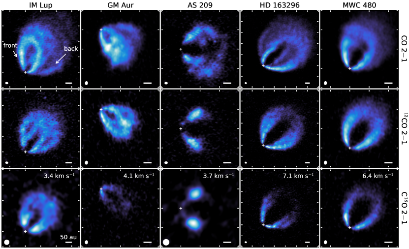
Figure 1: Representative channels for the MAPS sample, ordered from left to right by increasing stellar mass (see Table 1 in Oberg et al. (2021)), for CO 2–1, ¹³CO 2–1, and C¹⁸O 2–1. Both sides of the disk are visible and can be used to fit for the emitting layer. The C¹⁸O 2–1 images in IM Lup and GM Aur have been tapered to 0$\farcs$30, as described in Section 4.1. LSRK velocities are shown in the upper right corner and the plus symbol indicates the disk center. Axes are angular offsets from the disk center with 1^′′ tick marks. An arcsinh color stretch has been applied to highlight faint outer structures.

We derived emission surfaces using the disksurf Python package, which implements this method while providing additional functionality to filter the data to extract more precise emission surfaces. This series of filtering steps is described in detail in Appendix A. We used the get_emission_surface function to extract the deprojected radius $r$, emission height $z$, surface brightness I_ν, and channel velocity $v$ for each pixel associated with the emitting surface. These surfaces represent individual measurements, i.e., pixels, from the line image cubes.

We then use two different methods to further reduce scatter in the individual emission surface measurements and help better identify substructure. First, we radially bin the individual measurements using bin sizes of 1/4 of the FWHM of the beam major axis, i.e., the same as the radial intensity profiles in Law et al. (2021). The uncertainty is given by the standard deviation in each bin. We note that Pinte et al. (2018) included the uncertainty in the disk inclination in these uncertainties. We opted not to do this as the disk inclination is a systematic uncertainty and results in a scaling of the vertical height axis, and not a relative uncertainty between radial bins. Besides binning, we also calculated the moving average and standard deviation of the individual surface measurements. As the spacing between radial points is not uniform, we used a window size with a minimum size of one quarter of the FWHM of the beam major axis. This window was required to contain a fixed number of points, which means that the physical size that it represents changes with radius due to the non-uniform radial sampling from the deprojection process, i.e., in the less dense, outer disk, the window expands in order to still encompass this fixed number of points. A summary of these different data products is shown in Figure 2. While it was found that binned and moving average surfaces showed the same trends, the binned surface benefited from a uniform radial sampling, while the moving average retained a finer radial sampling, essential for identifying subtle perturbations associated with features in the dust continuum.

All three types of line emission surfaces — individual measurements, radially-binned, and moving averages — are provided as Value-Added Data Product (VADPs) and will be made available to the community through our dedicated website hosted by ALMA (https://almascience.nrao.edu/alma-data/lp/maps). See Section 7 for further details. Throughout this work, we sometimes bin these data products further for visual clarity, but all quantitative analysis is done using the original binning of each type of emission surface.

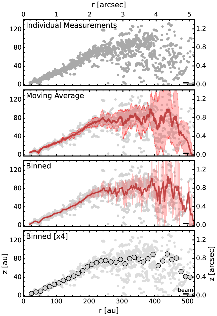
Figure 2: Comparison of emission heights derived for CO 2$-1$ in HD 163296 for individual measurements, moving average, and radially-binned surfaces (from top to bottom). For increased visual clarity, we occasionally bin surfaces by an extra factor of a few, as illustrated in the bottom panel. The FWHM of the major axis of the synthesized beam is shown in the bottom right of each panel.

3.2 Analytical Fits

To facilitate implementing these emission surfaces in models and for comparison with other observations, we fit an exponentially-tapered power law to all CO emission surfaces. This parametric fit was chosen as it describes the flared surface in the inner disk ($\lesssim$ 200 au) and captures the expected drop in the outer disk due to decreasing gas surface density, as seen in Figure 2. We adopt the following functional form:

$$z(r)=z_{0}\times\left(\frac{r}{1^{\prime\prime}}\right)^{\phi}\times\exp\left(-\left[\frac{r}{r_{\rm{taper}}}\right]^{\psi}\right)$$ (1)

where $z_{0}$, $\phi$, and $\psi$ should always be non-negative. A value of $\phi>1$ indicates that $z$ increases with radius, while $0<\phi<1$ tends toward a flat $z(r)$ profile. When $r_{\rm{taper}}\gg 1^{\prime\prime}$, $z_{0}$ represents the $z/r$ value at 1^′′. Note that some previous works, e.g., Teague et al. (2019), instead used a double power law profile to capture the drop in emission height at large radius. It was found that this tapered form, on average, provided a better fit to the data with less manual tuning required.

To ensure the robustness of these fits, we also restricted the radial range used for fitting to locations with high densities of $(r,\,z)$ measurements. The radial ranges used in each fit are given by $r_{\rm{fit,in}}$ and $r_{\rm{fit,out}}$ in Table 1.

Table 1: Parameters for Emission Surface Fits

Source	Line	Velocity Range	Exponentially-Tapered Power Lawa
		[km s-1]	$r_{\rm{fit,in}}$ [′′]	$r_{\rm{fit,out}}$ [′′]	$z_{0}$ [′′]	$\phi$	$r_{\rm{taper}}$ [′′]	$\psi$
IM Lup	CO 2$-$1	[2.8, 6.4]	0.21	3.26	4.37	3.144	0.254	0.655
	13CO 2$-$1	[2.6, 6.4]	0.61	2.02	0.159	2.599	1.928	4.993
GM Aur	CO 2$-$1	[3.1, 7.5]	0.08	3.36	0.385	1.066	3.767	4.988
	13CO 2$-$1	[3.7, 7.1]	0.2	1.89	0.113	4.539	1.496	4.989
	C18O 2$-$1	[$-$2.9, 13.9]	0.21	0.66	0.95	3.556	0.402	3.766
AS 209	CO 2$-$1	[2.9, 6.5]	0.07	1.98	0.219	1.292	1.786	4.854
	13CO 2$-$1	[2.9, 6.5]	0.73	1.35	0.175	2.98	1.124	2.445
HD 163296	CO 2$-$1	[4.3, 13.5]	0.19	4.73	0.388	1.851	2.362	1.182
	13CO 2$-$1	[3.5, 13.5]	0.31	3.42	0.121	1.503	3.158	4.996
	C18O 2$-$1	[3.5, 8.1]	0.39	1.43	0.174	2.956	1.043	4.994
MWC 480	CO 2$-$1	[2.8, 7.4]	0.13	3.69	0.261	1.35	3.098	3.074
	13CO 2$-$1	[2.8, 7.2]	0.05	2.26	1.248	2.165	0.215	0.683
	C18O 2$-$1	[$-$8.2, 18.2]	0.13	1.46	0.065	1.37	0.961	4.834

We used the Affine-invariant MCMC sampler (Goodman & Weare, 2010) implemented in emcee (Foreman-Mackey et al., 2013) to estimate the posterior distributions of these fits. We used 64 walkers which take 1000 steps to burn in and an additional 500 steps to sample the posterior distribution function. We chose an MCMC fitting approach rather than a simple chi-squared minimization to better handle the degeneracies between fitted parameters. Individual pixels are not all necessarily independent as they may originate within a single beam, which can lead to an underestimation of the true uncertainties on the extracted heights, i.e., on how well we can extract the mean $z$ from a sample of columns. However, this will not necessarily affect the mean height itself. This is analogous to drawing random samples from a normal distribution, where given a sufficiently large number of samples, the standard deviation of those samples provides a good estimate of the uncertainty on the mean of the distribution. Instead, if these samples are correlated and, e.g., that for every second draw, the sample is biased towards the one immediately preceding it, we will over-sample the central region compared to the wings. In this case, the standard deviation of the total ensemble will underestimate the true standard deviation of the distribution, but will not alter the underlying mean value.

The presence of this potential spatial correlation between pixels does not affect the analytical fits, which are instead dominated by overall radial trends rather than the vertical scatter in height measurements. Fits were also performed using the individual measurements, binned, and moving average surfaces, and we confirmed that all produced consistent results. We found that fits to the moving average surfaces were slightly more reliable at the outer disk radii. This is likely because the moving average is a compromise in terms of the number of radial points and relative signal-to-noise ratio (SNR), as the raw data have a finer grid of radial points but much larger scatter, while the binned data have coarser radial information but higher SNR.

The fitted $\phi$ (${\sim}$1.5-4) for the CO emission surfaces are often several times larger than the flaring indices of the gas pressure scale heights (1.08-1.35), which are derived by fitting the observed spectral energy distributions of each star+disk system (for more details, see Zhang et al., 2021). This difference was previously noted by Pinte et al. (2018) in IM Lup, who ascribed it to the sharp drop-off in UV radiation from the central star. The stellar irradiation determines the shape of the emitting surface, which follows a layer of approximately constant optical depth from the perspective of the star, rather than tracing the disk scale height. In particular, in the inner ${<}$300 au (${<}$120 au for AS 209) where the surfaces are still steeply rising, the CO surface originates from a height that is 2.5-3.5 times the scale height, while the ¹³CO and C¹⁸O surfaces are at approximately 1-1.5 scale heights. Similar values have been reported previously for IM Lup (Pinte et al., 2018), as well as in DM Tau (Dartois et al., 2003) and the Flying Saucer (Dutrey et al., 2017).

To further illustrate the geometry of the fitted surfaces, Figure 3 shows an overlay of the inferred emission surfaces on the peak intensity maps of CO 2–1 for all disks. Isovelocity contours generated using the surface fits from Table 1 for the CO isotopologues are also provided in Appendix B.

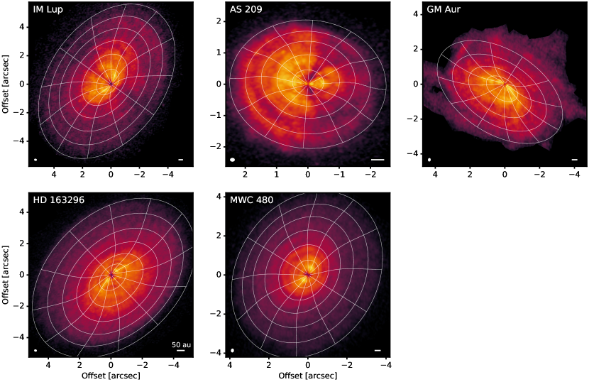
Figure 3: Peak intensity maps of CO 2–1 for all MAPS sources with overlaid contours showing the fitting emission surfaces, as listed in Table 1. The synthesized beam and a scale bar indicating 50 au is shown in the lower left and right corner, respectively, of each panel.

4 Results

4.1 Overview of Emission Surfaces

Figure 4 shows the surfaces derived for CO isotopologues in all disks. For each disk, the CO 2–1 surface lies higher than that of the ¹³CO 2–1, which, in turn, is higher than C¹⁸O 2–1. Such a progression is consistent with a line optical depth of ${\sim}$1 being reached at deeper layers for rarer isotopologues. There are considerable differences in the absolute surface heights of CO and ¹³CO between disks. For instance, the CO surface reaches a peak height of $z\approx$ 200 au in IM Lup and GM Aur, while they are below ${\sim}$100 au in AS 209, HD 163296, and MWC 480. A similar trend is seen in ¹³CO, where IM Lup has a maximum height of $z\approx$ 100 au, while AS 209 and MWC 480 peak at $z<$ 40 au. This range in absolute emission heights translates into a range of peak $z/r$. CO emission is present at $z/r\gtrsim 0.5$ in IM Lup and GM Aur, while $z/r\sim$ 0.2 in AS 209. ¹³CO shows less overall variation between disks than CO, and is generally present at $z/r<0.2$. C¹⁸O has $z/r\lesssim 0.1$ towards those disks where we had enough signal to estimate emission heights. Finally, the relationship among the CO, ¹³CO, and C¹⁸O emission heights within disks vary across the sample. In MWC 480, the CO emission surface is relatively elevated with $z/r\sim 0.3$, while ¹³CO and C¹⁸O are both very flat, i.e., $z/r<0.1$. By contrast, HD 163296 shows a gradual progression of $z/r\sim 0.3$ to $0.2$ to 0.1 for CO, ¹³CO and C¹⁸O, respectively.

No surfaces could be derived from the full resolution images of C¹⁸O 2–1 in IM Lup and AS 209 due to insufficient SNR. However, we were able to extract surfaces from the corresponding tapered (0$\farcs$30) image cubes (see Section 6.2, Czekala et al., 2021) but consider these to be tentative and did not attempt to fit analytical functions to these surfaces. Both are shown in Figure 4, but are otherwise omitted from subsequent analysis.

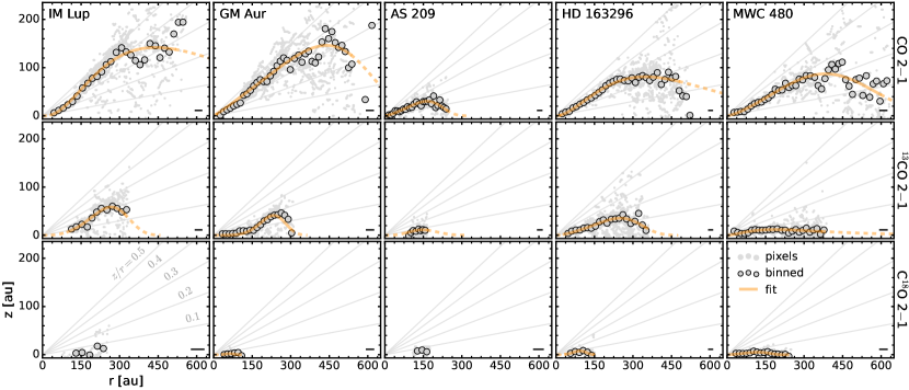
Figure 4: Emission surfaces for CO 2–1, ¹³CO 2–1, and C¹⁸O 2–1 in all MAPS sources. Large gray points show radially-binned surfaces and small, light gray points represent individual measurements. The orange lines show the exponentially-tapered power law fits from Table 1. The solid lines show the radial range used in the fitting, while the dashed lines are extrapolations. The C¹⁸O 2–1 surfaces in IM Lup and AS 209 are tentative and were derived from the tapered (0$\farcs$30) images. Lines of constant $z/r$ are shown in gray. The FWHM of the major axis of the synthesized beam is shown in the bottom right corner of each panel.

In all CO lines, except for CO in IM Lup, we see an initial increase of z/r with radius, i.e. flaring, a flattening, and then eventual turnover due to decreasing gas surface densities at large radii. IM Lup, which is known to possess extended diffuse CO emission (Cleeves et al., 2016), does not show clear evidence of this turnover and only shows moderate indications of flattening. All surfaces show some degree of vertical scatter, which is a combination of thermal noise in the images and potential azimuthal variations in the underlying emission surfaces. The relative contribution is, however, specific to each disk and emission line. As this scatter increases substantially with radius, the line SNR is likely the most important factor in setting the vertical scatter, at least at large radii. Due to different projections at varying azimuths in specific channels, the height of a particular pixel can often be easier or more difficult to determine, which provides an additional source of uncertainty in vertical pixel positions. For instance, channels with less favorable viewing geometries where the two disk sides cannot be easily distinguished make it harder to measure emission surface heights. This often occurs at velocities either very close to or substantially offset from the source systemic velocity. For example, in Figure 16, channels at larger velocity offsets (${\leq}$2.6 km s^-1 or ${\geq}$6.2 km s^-1) and those near the systemic velocity (${\approx}$ 4.5 km s^-1) show poorly-separated upper and lower disk surfaces.

Nonetheless, some surfaces appear more tightly constrained than others, i.e., CO in HD 163296 shows considerably less vertical dispersion compared to that of the MWC 480 disk. This scatter in the MWC 480 disk is not just due to noise, but is the result of localized azimuthal deviations. Perturbations in azimuthal velocity, on the order of a few %, are located at ${\sim}$240, 340, 370, and 450 au in MWC 480 (Teague et al., 2021), which approximately align with regions of prominent vertical scatter in its CO emission surface. Similarly detailed and disk-specific analyses are required to discern the origins of vertical scatter in the other MAPS sources. Several disks also show evidence of substructure in their surfaces, e.g., C¹⁸O in HD 163296, which we discuss in detail in Section 4.4.

Figure 5 shows the surfaces for C₂H and HCN. Of the disks around T Tauri stars, only surfaces for AS 209 could be extracted and appear to be at $z/r\lesssim 0.1$. The C₂H and HCN surfaces in IM Lup and GM Aur could not be reliably constrained due to their low line optical depths and SNRs compared to CO and ¹³CO. The two disks around Herbig Ae stars, HD 163296 and MWC 480, also show emission at a $z/r$ of 0.1 or less. In MWC 480, both HCN and C₂H are present at $z/r<0.1$, similar to the ¹³CO and C¹⁸O surfaces. HD 163296 is the only source where the C₂H and HCN lines show any structure; there is a clear gap in the surfaces corresponding to the gap between the two innermost rings in the radial emission profiles (Law et al., 2021). The first ring at 45 au is less vertically extended with $z/r<0.1$, while the emission in the second ring at 110 au is more elevated at $z/r\approx 0.1$. We do not attempt parametric fits for any of the HCN and C₂H lines.

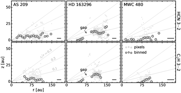
Figure 5: Emission surfaces for HCN 3–2 and C₂H 3–2 in AS 209, HD 163296, and MWC 480. Large gray points show radially-binned surfaces and small, light gray points represent individual measurements. Lines of constant $z/r$ are shown in gray. The FWHM of the major axis of the synthesized beam is shown in the bottom right corner of each panel. The HCN and C₂H surfaces for the remaining MAPS sources IM Lup and GM Aur lacked sufficient SNR for robust surface determinations.

4.2 Comparison with NIR rings

All of the MAPS sources have been observed in scattered light (Schneider et al., 2003; Kusakabe et al., 2012; Monnier et al., 2017; Avenhaus et al., 2018; Muro-Arena et al., 2018), which provides valuable information about the micron-sized dust grains in these disks. The IM Lup, AS 209, and HD 163296 disks have well-defined rings in the NIR, but only IM Lup and HD 163296 have direct estimates of their NIR emitting surfaces, as measured from individual rings. The inner NIR ring in HD 163296 has a height measured from Monnier et al. (2017), while the outer ring at 330 au was recently found to have a dust scale height of 64 au in NIR/HST observations (Rich et al., 2020). All four rings in IM Lup have measured NIR heights (Avenhaus et al., 2018). Figure 6 shows these NIR heights compared to the CO and ¹³CO 2–1 emission surfaces. We also plot the NIR emitting height relation identified in a sample of disks around T Tauri stars as part of the DARTTS-S program (Avenhaus et al., 2018) as a dashed red line in Figure 6.

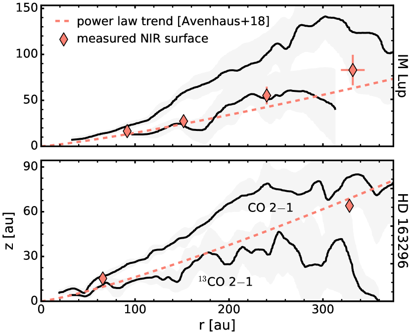
Figure 6: Emission surfaces of CO and ¹³CO 2–1 in IM Lup (top) and HD 163296 (bottom). The black lines are the moving average surfaces and gray shaded regions show the 1$\sigma$ uncertainty. The red diamonds show individual height measurements of NIR rings (Monnier et al., 2017; Avenhaus et al., 2018; Rich et al., 2020), while the red dashed line shows the inferred NIR surface using the relation found in a sample of disks in Avenhaus et al. (2018). The values from Monnier et al. (2017) have been scaled to reflect the updated Gaia distance for HD 163296. The errorbars are smaller than the marker for the innermost rings in both IM Lup and HD 163296 and the 330 au ring in HD 163296 does not have reported uncertainties.

The NIR surfaces lie between the CO and ¹³CO emitting layers in HD 163296, while in IM Lup, the NIR surface appears at approximately the same height as that of the ¹³CO, which is roughly consistent with the findings from Pinte et al. (2018) and Rich et al. (2021). Although lacking well defined rings, MWC 480 has been reported to have a very flat NIR surface, i.e., z/r$\sim$0.03 (Kusakabe et al., 2012), which suggests that the micron-sized dust lies at or below the ¹³CO and C¹⁸O emitting layers.

4.3 Gas temperatures

We can use line emitting surfaces together with line brightness temperatures to map disk temperature structures. When we extracted individual pixels from the image cubes, we also obtained a corresponding set of peak surface brightnesses. In Subsection 4.3.1, we describe how we converted these peak surface brightnesses into gas temperatures as a function of ($r$, $z$). Then, in Subsection 4.3.2, we present the radial temperature profiles and in Subsection 4.3.3, we analyze the full 2D empirical temperature structure of each disk. Both the radial temperature profiles and full ($r$, $z$) temperature structures for each MAPS are provided as publicly-available VADPs (see Section 7).

4.3.1 Calculating Gas Temperatures

The peak of the CO and ¹³CO 2–1 lines are expected to be optically thick with CO rotational levels in local thermodynamic equilibrium (e.g, Weaver et al., 2018) at the typical densities and temperatures of protoplanetary disks. Provided that the emission fills the beam, the peak surface brightness I_ν provides a measure of the temperature of the emitting gas. In order to not underestimate the line intensity along lines of sight containing optically thick continuum emission (e.g, Boehler et al., 2017; Weaver et al., 2018), we repeated the surface fitting, as in Section 3, using the non-continuum-subtracted image cubes (Czekala et al., 2021).

Each individual pixel ($r$, $z$) that was extracted has a peak surface brightness $I_{\nu}$, which was then used to calculate the associated gas temperature using the full Planck function:

$$T_{b}=\frac{h\nu}{k_{B}}\left[\ln\left(\frac{2h\nu^{3}}{c^{2}I_{\nu}}+1\right)\right]^{-1}$$ (2)

In addition to CO 2–1 and ¹³CO 2–1, we also calculated the brightness temperatures of C¹⁸O 2–1 in all disks and those of HCN 3–2 and C₂H 3–2 in HD 163296, but as we expect these lines to be partly optically thin, their brightness temperatures will be lower limits on the gas temperatures.

The western half of the AS 209 disk suffers from foreground cloud contamination (Öberg et al., 2011) in CO 2–1. Therefore, we calculated CO 2–1 temperatures using only the eastern half of the disk, which corresponds to the velocity range of 4.90 km s^-1 to 6.90 km s^-1 (see Appendix B), to avoid underestimating the peak brightness temperatures. For all other lines, we used the same velocity/channel ranges as in Table 1 for temperature calculations.

All subsequent radial and 2D gas temperature distributions represent those derived directly from individual surface measurements, rather than radially-deprojecting peak intensity maps (see Teague et al., 2021) or mapping peak brightness temperatures back onto derived emission surfaces (i.e., Figure 3). We only consider the brightness temperatures of those pixels where we were able to determine an emission height.

4.3.2 Radial temperature distributions

Figure 7 shows the radial temperature profiles for the CO isotopologues. We first reiterate that these temperatures are measurements of surface brightnesses, rather than integrated intensities that are used to identify line emission substructures (Law et al., 2021) or derive column densities (Zhang et al., 2021). As expected, in each disk, CO is the warmest, followed by ¹³CO and then C¹⁸O. CO displays the largest range of measured temperatures, while ¹³CO and C¹⁸O span a more limited range. The radial temperature gradients are consistent within each disk with similar slopes across CO isotopologues with the exception of AS 209, where the ¹³CO is nearly flat over the entire radial range in which it was measured. This flatness in temperature structure is due to the ¹³CO emission rings in AS 209 and in this case, we are only able to derive the brightness temperature of the outer ring at ${\sim}$120 au (Favre et al., 2019; Law et al., 2021).

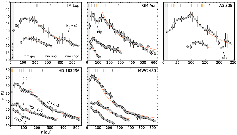
Figure 7: Radial brightness temperature profiles for CO 2–1, ¹³CO 2–1, and when available, C¹⁸O 2–1. The top and bottom rows are each shown on a consistent temperature scale and are grouped by whether the host star is a T Tauri or Herbig Ae star, respectively. These profiles represent the mean temperatures computed by radially binning the individual measurements, similar to the procedure used to compute the radially-binned surfaces (see Section 4.3.1). Vertical lines show the 1$\sigma$ uncertainty, given as the standard deviation of the individual measurements in each bin. For increased visual clarity, all disks have been binned by an extra factor of two, except for IM Lup and HD 163296, which have been binned by an additional factor of three and four, respectively. The solid red line shows the fitted power law profile from Table 2. The inner gray shaded region is the FWHM of beam major axis. The orange and gray dashes correspond to the mm continuum rings and gaps, respectively. The black dots mark the outer edge of the millimeter continuum. Temperature dips in GM Aur, AS 209, and HD 163296 are labeled with arrows, as is a temperature bump in IM Lup.

The disks around T Tauri stars have brightness temperatures spanning ${\sim}$10–40 K. The disks around Herbig Ae stars HD 163296 and MWC 480 are generally warmer at a given radius and have an overall larger total temperature range from ${\sim}$10–70 K. The CO 2–1 temperatures are about 10 K higher in MWC 480 than in HD 163296, with the greatest differences occurring within ${<}$200 au. In particular, the HD 163296 and MWC 480 profiles are consistent with those presented in Teague et al. (2021), which were instead generated by deprojecting the peak intensity maps rather than direct extraction from emitting surfaces. Likewise, the CO 2–1 temperature profile of HD 163296 is approximately consistent with, although slightly cooler than, the one derived from a similar direct extraction method in Isella et al. (2018). We note that brightness temperatures less than 20 K are below the CO freeze-out temperature, which suggests that the associated line emission is at least partially optically thin and thus only provides a lower limit on the true gas temperatures. This conclusion is supported by our data, where CO lines with ${<}$20 K are most common for the rarer isotopologues and at large disk radii.

The drop in brightness temperature seen within 20–40 au in all disks and lines, which is marked as a shaded region in Figure 7, is due to beam dilution as the emitting area becomes comparable to or smaller than the angular resolution of the observations. In the case of IM Lup and AS 209, the central temperature dip extends further than the beam size. This may suggest enough CO depletion for the lines to become optically thin at these innermost radii, unresolved CO emission substructure, or that a substantial fraction of the CO emission is absorbed by dust. Indeed, Cleeves et al. (2016) and Sierra et al. (2021) find that the dust is optically thick in the inner regions of the IM Lup disk, and Bosman et al. (2021) also see a large CO emission gap which is best explained by dust absorption. Dust absorption may also contribute to the low CO temperature in the inner AS 209 disk, but not out to 100 au. Optically thin emission is also an unlikely explanation: Zhang et al. (2021) finds that while AS 209 has a lower CO surface density than all other MAPS disks, it is still far from the optically thin limit in CO 2-1. This leaves CO substructure as an explanation. AS 209 does present several gaps in CO emission interior to 100 au (Guzmán et al., 2018; Law et al., 2021; Zhang et al., 2021; Bosman et al., 2021), which are barely resolved and may therefore result in a low brightness temperature in the inner disk.

Figure 7 also shows the locations of millimeter continuum gaps and rings, as reported in Law et al. (2021). The radial temperature profiles are quite smooth and hence the opportunity for coincidences between temperature substructures and other substructures is small. In two cases, the temperature substructure that is seen does line up with known disk substructures, however. HD 163296 has a 5 K drop in temperature at ${\sim}$80-90 au in all three CO lines, which aligns with a gap at 85 au in the millimeter continuum. A similar drop in temperature at ${\sim}90$ au is also present in CO in GM Aur, which roughly aligns with a gap-ring pair at 68 au and 86 au in the millimeter continuum. In AS 209, a slightly deeper (${\sim}$8 K) drop occurs at 200 au in CO 2–1 and is coincident with a CO 2–1 line emission gap at 197 au (Law et al., 2021). Low-amplitude (${\sim}$2-3 K) wave-like fluctuations are seen in CO 2–1 temperature in MWC 480 (for further discussion of the features, see Teague et al., 2021). We find no association between temperature trends and the outer continuum edge in GM Aur and AS 209, but do notice a modest flattening of the CO temperature gradient at the edge of the millimeter continuum in HD 163296 and MWC 480. Although about 50 au beyond the continuum edge, the CO 2–1 temperature in IM Lup shows a modest increase at 450 au. This may be associated with a temperature inversion in the midplane (Cleeves, 2016) and is broadly consistent with the radial location of 400 au predicted in the models of Facchini et al. (2017).

We fitted the temperature profiles with power laws as:

$$T=T_{100}\times\left(\frac{r}{\rm{100\,au}}\right)^{-q}$$ (3)

We first visually chose the radial range in which the temperature profiles behave like a power law and then fitted each profile using the Levenberg-Marquardt minimization implementation in scipy.optimize.curve_fit. The fitting ranges and derived parameters are listed in Table 2.

Table 2: Radial Temperature Profile Fits

Source	Line	rfit,in [au]	rfit,out [au]	T100 [K]	q
IM Lup	CO 2$-$1	170	559	55 $\pm$ 0.9	0.58 $\pm$ 0.01
	13CO 2$-$1	145	339	30 $\pm$ 0.6	0.32 $\pm$ 0.03
GM Aur	CO 2$-$1	135	613	52 $\pm$ 0.9	0.61 $\pm$ 0.02
	13CO 2$-$1	50	314	22 $\pm$ 0.2	0.26 $\pm$ 0.01
	C18O 2$-$1	30	126	14 $\pm$ 0.4	0.38 $\pm$ 0.05
AS 209	CO 2$-$1	95	244	42 $\pm$ 1.0	0.78 $\pm$ 0.05
	13CO 2$-$1	125	163	28 $\pm$ 1.3	0.80 $\pm$ 0.13
HD 163296	CO 2$-$1	150	527	78 $\pm$ 1.0	0.82 $\pm$ 0.01
	13CO 2$-$1	50	356	31 $\pm$ 0.2	0.37 $\pm$ 0.01
	C18O 2$-$1	40	148	21 $\pm$ 0.3	0.37 $\pm$ 0.03
MWC 480	CO 2$-$1	100	632	70 $\pm$ 1.1	0.69 $\pm$ 0.02
	13CO 2$-$1	100	388	42 $\pm$ 0.9	0.60 $\pm$ 0.03
	C18O 2$-$1	80	251	26 $\pm$ 0.2	0.75 $\pm$ 0.02

As shown in Figure 7, these fits work well beyond ${\sim}$100–150 au in all disks but overpredict the measured brightness temperatures interior to this. The temperature profile of CO in MWC 480 changes slope at approximately 350 au, which complicates the choice of radial fitting range. It is possible to achieve a modestly more accurate fit if instead two power laws are used, one for the inner disk between 40 and 200 au and another for the outer disk from ${>}135$ au. However, for simplicity, we fit a single power to the maximal possible range.

In addition to the CO lines, we also derived the brightness temperature profiles of HCN and C₂H in HD 163296, as shown in Figure 8. The shapes of the temperature profiles are consistent but offset, as HCN is warmer by 4–6 K at all radii. The gap at ${\sim}$80 au has a C₂H temperature of ${<}15$ K and HCN temperature of ${<}20$ K. Both lines seem to be cooler near the gap by a few K relative to the outer ring and by almost 10 K versus the inner ring. However, the beam filling factor will be reduced at locations closer to the gap, likely becoming significant within 1/2 – 1 beams away. Thus, the line emission near this gap may become increasingly optically thin. In this case, the lower brightness temperatures would reflect reduced gas density, rather than cooler HCN and C₂H gas temperatures. Overall, the HCN brightness temperatures are consistent with the excitation temperatures derived in the multi-line analysis of Guzmán et al. (2021). However, the C₂H temperatures are a factor of two lower than those reported in Guzmán et al. (2021), which suggests that the C₂H 3–2 line is optically thin or not in local thermal equilibrium (LTE). Thus, a non-LTE analysis of C₂H in HD 163296 is warranted.

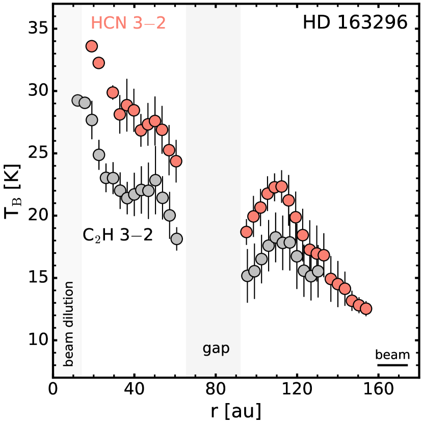
Figure 8: Radial brightness temperature distributions of HCN 3–2 and C₂H 3–2 in HD 163296. These profiles represent the mean temperatures computed by radially binning the individual measurements, similar to the procedure used to compute the radially-binned surfaces (see Section 4.3.1). Vertical lines show the 1$\sigma$ uncertainty, given as the standard deviation of the individual measurements in each bin. The gap location seen in the line emission (Law et al., 2021) is labeled and shaded in gray. The FWHM of the beam major axis is shown in the lower right corner and also indicated by the inner gray shaded region.

4.3.3 2D temperature structure

The advantage of having multiple CO isotopologues that trace different disk heights is access to the vertical temperature distribution. Dartois et al. (2003) were the first to demonstrate this in moderate resolution (${\sim}$1^′′) observations of DM Tau. More recently, Pinte et al. (2018) presented a framework for directly mapping the temperature structure of each emitting layer in (${\sim}$0$\farcs$4) observations of IM Lup. Here, we expanded this analysis to the high spatial resolution observations of the MAPS disks. Figure 9 shows the full 2D temperature distributions.

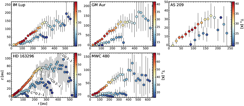
Figure 9: 2D temperature distributions of CO 2–1, ¹³CO 2–1, and when available, C¹⁸O 2–1 in all MAPS sources. Points are those from the binned surfaces and error bars are the 1$\sigma$ uncertainties in $z$. For some of the innermost points, the uncertainty is smaller than the marker. Data for all disks and lines have been binned by a factor of three for visual clarity. The uncertainty of the temperature measurements, which is not shown here, can be found in Figure 7.

Since we have temperature information as a function of $(r\,,z)$, we can construct a full 2D model of the temperature distribution of each disk. To do so, we adopt a two-layer model similar to the one proposed by Dartois et al. (2003), but then modified by Dullemond et al. (2020) with a different connecting term. Both formula were initially tried but substantially better fits were obtained with that of Dullemond et al. (2020). The midplane temperature $T_{\rm mid}$ and atmosphere temperature $T_{\rm atm}$ are assumed to have a power-law profile with slopes $q_{\rm mid}$ and $q_{\rm atm}$, respectively.

$$T_{\rm{atm}}(r)=T_{\rm{atm},0}\left(r/100~{}\rm{au}\right)^{q_{\rm{atm}}}$$ (4)

$$T_{\rm{mid}}(r)=T_{\rm{mid},0}\left(r/100~{}\rm{au}\right)^{q_{\rm{mid}}}$$ (5)

Between the midplane and atmosphere, the temperature is smoothly connected using a tangent hyperbolic function

$$T^{4}(r,z)=T^{4}_{\rm{mid}}(r)+\frac{1}{2}\left[1+\tanh\left(\frac{z-\alpha z_{q}(r)}{z_{q}(r)}\right)\right]T^{4}_{\rm{atm}}(r),$$ (6)

where $z_{q}(r)=z_{0}\left(r/100~{}\rm{au}\right)^{\beta}$. We note that the $\alpha$ parameter defines where in height the transition in the tanh vertical temperature profile occurs and $\beta$ describes how the transition height varies over radius. In total, we fitted the following seven parameters: $T_{\rm atm,0}$, $q_{\rm atm}$, $T_{\rm mid,0}$, $q_{\rm mid}$, $\alpha$, $z_{0}$, and $\beta$.

We performed the fitting using MCMC with emcee (Foreman-Mackey et al., 2013) with 256 walkers which take 500 steps to burn in and an additional 5000 steps to sample the posterior distribution function. All available CO lines were fitted using the individual measurements and only those points with $T_{\rm{B}}>20$ K were considered. Temperatures below 20 K, close to the CO freeze-out temperature, are likely optically thin and thus not useful for constraining the gas temperature structure. Parameter values and associated uncertainties are taken to be the 50th, 16th, and 84th percentiles from the marginalized posterior distributions, respectively, and are listed in Table 3.

Table 3: Summary of 2D Temperature Structure Fits

Source	$T_{\rm{atm},0}$ [K]	$T_{\rm{mid},0}$ [K]	$q_{\rm{atm}}$	$q_{\rm{mid}}$	$z_{0}$ [au]	$\alpha$	$\beta$
IM Lup	36${}^{+0.1}_{-0.1}$	25${}^{+0.1}_{-0.1}$	0.03${}^{+0.01}_{-0.01}$	$-$0.02${}^{+0.01}_{-0.01}$	3${}^{+0.1}_{-0.1}$	4.91${}^{+0.17}_{-0.16}$	2.07${}^{+0.02}_{-0.02}$
GM Aur	48${}^{+0.3}_{-0.3}$	20${}^{+0.2}_{-0.2}$	$-$0.55${}^{+0.01}_{-0.01}$	$-$0.01${}^{+0.01}_{-0.01}$	13${}^{+0.2}_{-0.2}$	2.57${}^{+0.03}_{-0.03}$	0.54${}^{+0.01}_{-0.01}$
AS 209	37${}^{+0.2}_{-0.2}$	25${}^{+0.2}_{-0.2}$	$-$0.59${}^{+0.02}_{-0.02}$	$-$0.18${}^{+0.01}_{-0.01}$	5${}^{+0.2}_{-0.2}$	3.31${}^{+0.12}_{-0.11}$	0.02${}^{+0.02}_{-0.02}$
HD 163296	63${}^{+0.2}_{-0.2}$	24${}^{+0.1}_{-0.1}$	$-$0.61${}^{+0.003}_{-0.003}$	$-$0.18${}^{+0.004}_{-0.004}$	9${}^{+0.1}_{-0.1}$	3.01${}^{+0.02}_{-0.02}$	0.42${}^{+0.004}_{-0.004}$
MWC 480	69${}^{+0.2}_{-0.2}$	27${}^{+0.2}_{-0.2}$	$-$0.7${}^{+0.004}_{-0.004}$	$-$0.23${}^{+0.01}_{-0.01}$	7${}^{+0.1}_{-0.1}$	2.78${}^{+0.02}_{-0.02}$	$-$0.05${}^{+0.01}_{-0.01}$

The 2D fitted models are shown in comparison with the data in Figure 10. For all disks, the median residuals between the fitted model and measured temperatures are typically no more than 10%. The most informative fits are those with a well-sampled $(r,\,z)$ space, which means that we have a set of CO isotopologue lines with a diverse set of $z/r$ values, e.g., HD 163296. In contrast, IM Lup is poorly constrained over the height of the disk, since surfaces were only able to be determined for CO and ¹³CO and they are not widely spaced in $z/r$. The abrupt change in $z/r$ from CO to ¹³CO and C¹⁸O in MWC 480 is also reflected in its inferred 2D temperature structure by its small fitted $\alpha$ and $\beta$ values (Table 3). This means that the transition in vertical temperature, as described in Equation 6, occurs close to the midplane and the transition height does not increase over radius, unlike other disks. In general, as the emitting surfaces do not provide direct constraints in the disk midplanes, we caution the use of the empirically derived $T_{\rm{mid}}$, which are considerably warmer than predictions from thermo-chemical models (Zhang et al., 2021).

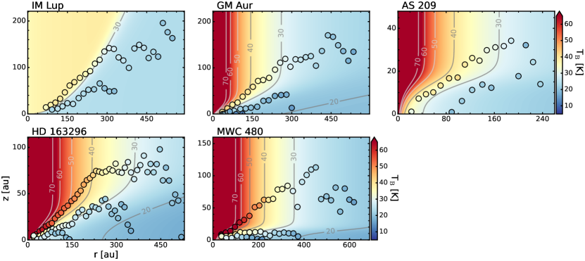
Figure 10: Comparison of the measured temperatures (points) with the fitted 2D temperature structures (background), as listed in Table 3. The same color scale is used for the data and fitted model and is consistent across all panels. Contours show constant temperatures in increments of 10 K. Data for all disks and lines have been binned by a factor of three for visual clarity. The uncertainty of the temperature measurements, which is not shown here, can be found in Figure 7.

4.4 Substructures in emission surfaces

Localized vertical substructures are observed in many of the emission surfaces derived from the MAPS data. The properties of these substructures, namely their radial locations, widths, and depths, provide important constraints that are necessary for detailed thermo-chemical modelling (e.g., Rab et al., 2020; Calahan et al., 2021). In the following subsections, we identify and catalogue all substructures present in the derived emitting layers and compare them with the gas temperature profiles, and with substructures observed in the millimeter continuum and CO line emission.

4.4.1 Fitting vertical substructures

Each substructure is labeled with its radial location rounded to the nearest whole number in astronomical units and is preceded with “Z” to indicate these features are vertical variations. This nomenclature is also chosen to avoid ambiguity with that used to denote radial substructures in the continuum (Huang et al., 2018) and molecular line emission (Law et al., 2021) profiles, which labels rings by “B” (“bright”) and gaps by “D” (“dark”).

Feature identification was done visually and focused on the inner, rising portion of the surfaces within ${\sim}$200 au, which was the most well-constrained and possessed the highest SNRs. We used the moving average surfaces to search for substructures in the form of vertical dips, i.e., we assumed that substructures represent localized decreases in $z$ in an otherwise smoothly-varying emitting layer. To fit each substructure, we first visually estimated a local baseline. This baseline was then fitted with a quadratic polynomial and subtracted from the original emitting surface. The derived properties of each feature will depend on the assumed form of the local baseline, but a low-order polynomial baseline is sensible for the inner ${<}200$ au of each disk. We then fitted a Gaussian profile to characterize each feature in the baseline-subtracted surface. An example of this fitting process for CO 2–1 in HD 163296 is shown in Figure 11.

The fitted centers and FWHMs of each Gaussian are taken to be the radial location and widths of each feature, respectively. Substructure depths are defined as $\Delta z$/$z_{\rm{baseline}}$, where $z_{\rm{baseline}}$ is the vertical height of the fitted baseline and $\Delta z$ is the fitted vertical height of the emitting surface at the radial position of the substructure. Depths are subsequently referred to according to their fractional decrease in vertical height with deeper features having lower height ratios, e.g., the Z46 in HD 163296 has a $\Delta z$/$z_{\rm{baseline}}=0.52$, which indicates a depth of 48%. The center, width, and relative depth of each feature is listed in Table 4 and their radial locations are labeled in Figure 12.

The relative depth of each feature is sometimes more uncertain than Table 4 suggests, as depth strongly depends on the assumed baseline, but overall, we find that this method works well to identify substructure radial locations and provides a preliminary characterization. These definitions also do not explicitly account for beam effects. In a few cases, the widths and depths of individual features are smaller than the minor axis of the beam FWHM. However, this is not generally a concern, as surfaces are derived from the positional offsets of peak intensities, which are sensitive to scales smaller than the beam size.

Typical feature depths range from ${\sim}$30–70% and widths from 10–50 au. HD 163296 has the largest total number of identified substructures, which are relatively narrow (${\sim}$10–15 au), while those in IM Lup and MWC 480 have broader widths (${\sim}$30–50 au). A consistent broad, bowl-shaped depression is seen in all CO lines in MWC 480 around 66 au with a width of ${\gtrsim}$30–40 au and depth of 40–60%. The two features Z170 and Z375 associated with IM Lup are notable, as they occur at the largest radii of all identified substructures. Although having modest relative depths of 68% and 49%, they possess an absolute $\Delta$z of 46 and 18 au, which are the largest in au by a factor of a few to an order of magnitude compared to all other substructures. Features are not always present across all CO isotopologues. For instance, Z170 in IM Lup is only seen in ¹³CO but not in CO, while in HD 163296, Z81 and Z83 are present in ¹³CO and C¹⁸O, respectively, but no corresponding feature is identified in CO.

In addition to the isolated, Gaussian-like dips we report above, we detect a few more complex trends. For instance, prominent changes in the slope of the emission surface are present at ${\sim}$150 au in ¹³CO in GM Aur and at ${\sim}$115 au in CO in IM Lup. Both AS 209 and MWC 480 also show large-scale, wave-like patterns in their CO surfaces with peak-to-trough separations of roughly 20 au and 40 au, respectively and amplitudes of no more than a few au. Thus, Z56 in AS 209 and Z66 in MWC 480 may in fact be local minima associated with this larger wave rather than separate isolated substructures.

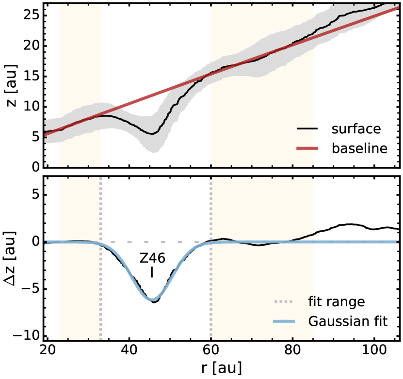
Figure 11: Example of the vertical substructure fitting process in the CO 2–1 emission surface of HD 163296. The top panel shows the removal of a local baseline (solid red line) in the form of a quadratic polynomial fit. The bottom panel shows a Gaussian fit (solid blue line) to the Z46 substructure in the baseline-subtracted emission surface. The radial range for the local baseline was visually identified and is shown by the orange shaded regions.

Table 4: Properties of Vertical Substructures

Source	Line	Feature	$r_{0}$ [arcsec]	$r_{0}$ [au]	Width [arcsec]	Width [au]	$\Delta$z [arcsec]	$\Delta$z [au]	Deptha
IM Lup	CO 2$-$1	Z375	2.38 $\pm$ 0.03	375 $\pm$ 5	0.18 $\pm$ 0.09	29 $\pm$ 14	0.29 $\pm$ 0.1	46 $\pm$ 16	0.32 $\pm$ 0.28
	13CO 2$-$1	Z170	1.08 $\pm$ 0.01	170 $\pm$ 2	0.18 $\pm$ 0.002	29 $\pm$ 0.4	0.11 $\pm$ 0.004	18 $\pm$ 1	0.51 $\pm$ 0.49
AS 209	CO 2$-$1	Z56	0.47 $\pm$ 0.02	56 $\pm$ 2	0.1 $\pm$ 0.01	13 $\pm$ 1	0.03 $\pm$ 0.02	4 $\pm$ 2	0.33 $\pm$ 0.18
HD 163296	CO 2$-$1	Z46	0.45 $\pm$ 0.01	46 $\pm$ 1	0.11 $\pm$ 0.01	12 $\pm$ 1	0.06 $\pm$ 0.01	6 $\pm$ 1	0.52 $\pm$ 0.13
	13CO 2$-$1	Z49	0.48 $\pm$ 0.02	49 $\pm$ 2	0.1 $\pm$ 0.003	11 $\pm$ 0.3	0.02 $\pm$ 0.004	2 $\pm$ 0.4	0.36 $\pm$ 0.03
		Z81	0.8 $\pm$ 0.001	81 $\pm$ 0.1	0.11 $\pm$ 0.03	12 $\pm$ 3	0.05 $\pm$ 0.03	5 $\pm$ 4	0.43 $\pm$ 0.24
		Z145	1.43 $\pm$ 0.01	145 $\pm$ 1	0.1 $\pm$ 0.01	10 $\pm$ 1	0.02 $\pm$ 0.03	2 $\pm$ 3	0.33 $\pm$ 0.28
	C18O 2$-$1	Z83	0.82 $\pm$ 0.004	83 $\pm$ 0.4	0.16 $\pm$ 0.02	16 $\pm$ 2	0.06 $\pm$ 0.001	6 $\pm$ 0.1	0.66 $\pm$ 0.02
MWC 480	CO 2$-$1	Z66	0.41 $\pm$ 0.01	66 $\pm$ 1	0.19 $\pm$ 0.04	31 $\pm$ 7	0.04 $\pm$ 0.003	7 $\pm$ 1	0.42 $\pm$ 0.06
	13CO 2$-$1	Z66	0.41 $\pm$ 0.06	66 $\pm$ 9	0.28 $\pm$ 0.04	46 $\pm$ 7	0.03 $\pm$ 0.02	6 $\pm$ 4	0.63 $\pm$ 0.09
	C18O 2$-$1	Z71	0.44 $\pm$ 0.03	71 $\pm$ 5	0.32 $\pm$ 0.06	51 $\pm$ 9	0.03 $\pm$ 0.003	4 $\pm$ 0.5	0.63 $\pm$ 0.55

4.4.2 Comparison with gas temperature

Since we have estimates for the gas temperatures, we also searched for coincidences between vertical and temperature substructures, but only found a single one, i.e., Z81 in ¹³CO in HD 163296. In IM Lup, the outer edge of the CO temperature plateau occurs around 180 au, which is roughly coincident with the Z170 feature seen in the ¹³CO surface. The CO 2–1 radial temperature profiles and emitting surfaces in MWC 480 also both show wave-like patterns, which are very roughly coincident in radial location. For further discussion of these features, see Teague et al. (2021). Otherwise, no other temperature trends are identified in any of the CO lines in the MAPS disks. Thus, the empirical gas temperatures do not generally seem to be sensitive to the presence of surface substructures. This may be explained, in part, due to deeper layers in the disk being more isothermal than the upper layers. Thus, a small change in the emission height would look like a bigger dip in temperature for CO than ¹³CO, for instance. Moreover, since the scale height is proportional to $\sqrt{T}$, this means that significant temperature differences are required for noticeable changes in the scale height.

4.4.3 Comparison with millimeter continuum and line emission substructures

The majority of the MAPS disks show at least some spatial links between vertical substructures and either continuum or radial substructure in CO line emission, as shown in Figure 12. Below, we consider each of these possible spatial associations.

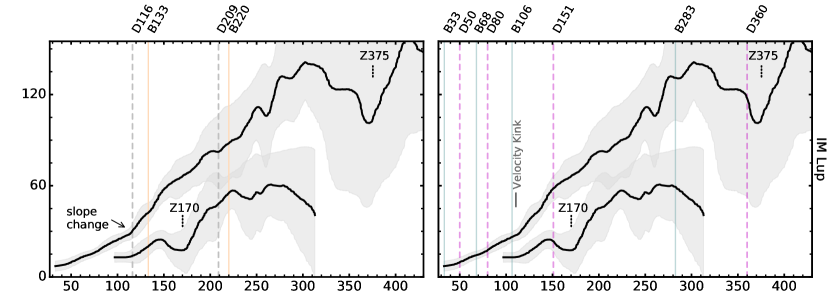
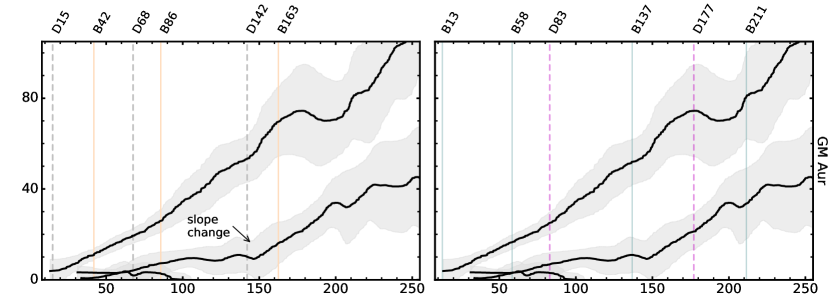
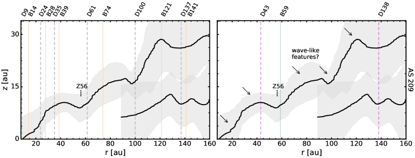
Figure 12: Comparison of CO 2–1, ¹³CO 2–1, and C¹⁸O 2–1 (when available) surfaces with annular substructures in the millimeter continuum (left) and CO line emission (right). Substructures are labeled following the nomenclature of Huang et al. (2018) and taken from Law et al. (2021). The CO line emission substructures are from CO 2–1 for all disks, except for MWC 480, which show those from ¹³CO 2–1. Substructures are labeled as follows: dust ring (solid orange line), dust gap (dashed gray line), chemical ring (solid blue line), and chemical gap (dashed purple line). Dotted black lines mark vertical substructures, as listed in Table 4. Notable changes in emitting surface slope and the suggestive wave-like features in AS 209 and MWC 480 are marked with arrows. The CO velocity kinks from Pinte et al. (2018, 2020) are labeled in IM Lup and HD 163296.

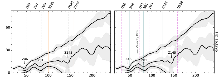
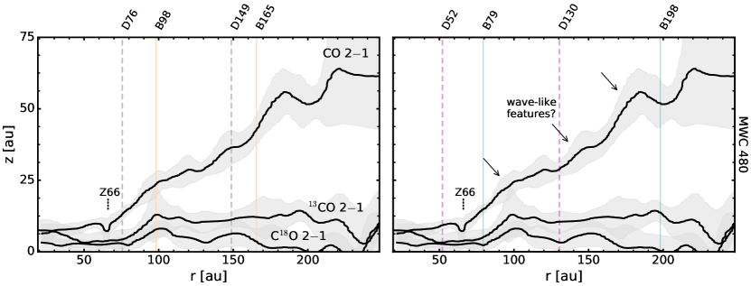
Figure 12: Continued.

All MAPS disks show some degree of spatial association between surface features and millimeter continuum substructures. Each dust gap in HD 163296 aligns with a surface feature in at least one of the CO isotopologue surfaces and in the case of ¹³CO, there is a one-to-one match between millimeter gaps and surface substructures. In MWC 480, the inner dust gap D76 roughly aligns with the Z66 surface feature and the outer dust gap at D149 approximately matches the location of the 140 au trough of the wave-like fluctuations. However, these associations in MWC 480 are considerably more tentative and considering that the surface features are more than twice the width of continuum gaps, these may be chance alignments. Several of the wave-like surface features in AS 209 align with the radial locations of substructures in the millimeter continuum. In particular, Z56 and the troughs at ${\sim}$100 and 140 au are radially coincident with dust gaps. The changes in emitting surface slope in CO 2–1 in IM Lup and ¹³CO 2–1 in GM Aur are also both co-located with the D116 and D142 dust gaps, respectively.

In a few cases, we identify features in the CO line emission profiles that are radially coincident with vertical substructures. In HD 163296, the CO line emission peaks at B49 and B81 directly align with the vertical substructures at Z49 and Z81, respectively. The CO peak at B59 is also co-located with the Z56 feature in AS 209. Both changes in slope in IM Lup and GM Aur are spatially associated with CO features at B106 and B137, respectively. In IM Lup, we also find that the D360 gap in line emission may be spatially related to the Z375 vertical dip. Given that both line emission peaks and gaps show some spatial association with surface substructures, this may point toward multiple mechanisms producing these surface features.

5 Discussion

5.1 Comparison to previous results

Pinte et al. (2018) were the first to demonstrate an approach to directly extract CO emission surfaces in moderate resolution observations of IM Lup. Similar methods were then used by Teague et al. (2018a, b, 2019) and Rich et al. (2021) to constrain the emitting layers in AS 209 and HD 163296. Below, we compare these previous results to the high spatial resolution MAPS observations and comment on the relatively consistency and any salient differences.

5.1.1 IM Lup

Pinte et al. (2018) found CO and ¹³CO 2–1 emission heights of $z/r\approx 0.325$ and $z/r\approx 0.125$ in the inner flared disk region, i.e., $r<300$ au, using ${\sim}$0$\farcs$4 resolution observations. In this same region, we find a considerably more elevated CO surface of $z/r\gtrsim 0.5$ and ¹³CO of $z/r\approx 0.2$. The differences in the derived heights are likely the result of our improved angular resolution, allowing for better separation of the front and back disk sides, e.g., see Figure 17, which demonstrates the limitations of poorer spatial resolutions. Pinte et al. (2018) also found that the CO 2–1 surface flattens out beyond 300 au, while our higher sensitivity observations reveal that this is due to a local minimum (Z375), and that globally the CO surface continues to rise out to 550 au due to diffuse large radii CO emission (e.g., Cleeves et al., 2016). Pinte et al. (2018) do not detect vertical substructures in any of their CO surfaces, but this is likely a consequence of their modest spatial resolution.

We also find consistent brightness temperature distributions to those of Pinte et al. (2018), but with overall systematically warmer temperatures by ${\sim}$5 K. This systematic offset is likely due to beam dilution in Pinte et al. (2018) whose larger beam (${\sim}4\times$) would have smeared out some of this emission. Overall, these comparisons illustrate the importance of high spatial resolutions in accurately constraining emission surfaces. At more moderate spatial resolution, estimates of the heights of emitting layers and gas temperatures are both underestimated. A detailed exploration of the effect of spatial resolution on extracted surfaces within the MAPS disk is found in Appendix D. In short, we find that surfaces derived from images with beam sizes between 0$\farcs$12 and 0$\farcs$2 are consistent, suggesting that the results presented here are not underestimated due to insufficient angular resolutions.

Rich et al. (2021) fit the CO 2–1 emission surfaces in the IM Lup disk using the DSHARP datacubes (Andrews et al., 2018) with a similar extraction method. These images have a spatial resolution of ${\sim}$0$\farcs$12, which is comparable to the MAPS resolution. Their CO 2–1 surface is nearly identical to the one we derived with the MAPS data and shows the same slope change at ${\sim}$110 au and a localized dip around 375 au.

5.1.2 AS 209

Teague et al. (2018b) derived the CO 2–1 emission surface in the AS 209 disk using the same approach as Pinte et al. (2018) using high spatial resolution (${\sim}$0$\farcs$2) CO line data. The authors found a surface with $z/r\sim 0.2$, which is the same $z/r$ we derived. However, they find a continually rising surface out to 300 au, but our surface begins to plateau and turnover at ${\gtrsim}$150 au. This difference may be due to their factor of two coarser spatial resolution. Teague et al. (2018b) also model the CO 2–1 emission surface that best reproduces the observed deviations in rotation velocities. Unlike the directly mapped surface, which is mostly smooth, the modeled surface has wave-like vertical substructures that appear very similar to those seen in the MAPS CO 2–1 emitting surface.

5.1.3 HD 163296

Teague et al. (2019) mapped the CO 2–1 emission surface in the HD 163296 disk at an angular resolution of ${\sim}$0$\farcs$1. The authors constrained an emission surface out to a radius of 4^′′ that is nearly identical to one that we derive. In the same disk but using lower resolution observations (${\sim}$0$\farcs$25), Teague et al. (2018a) modeled the emitting layer of C¹⁸O 2–1 as a Gaussian process and found a typical $z/r\approx 0.1$, consistent with our C¹⁸O surface. Teague et al. (2018a) also found slight dips in their emission surface at the millimeter gap locations, i.e., ${\sim}$50, 80, 130 au (once rescaled to the Gaia distance). The first two depressions correspond to the Z49 and Z81 dips in our surface, while the 130 au dip lies beyond the turnover region in our data. The discrepancy at large radii between these surfaces may be due in part to their larger beam size (about twice that of the MAPS beam) as well as a different approach to surface extraction. Nonetheless, they are still broadly consistent with one another.

Rich et al. (2021) also used the DSHARP images (${\sim}$0$\farcs$1) to extract the CO 2–1 surface of HD 163296. The authors find a surface that is very consistent, i.e., $z/r\approx 0.35$, with that derived from the MAPS data. However, the authors do not resolve the inner dip at 46 au that is clearly seen in the MAPS surfaces.

5.2 Origins of emission layer heights

While the majority of emitting surfaces show a consistent general behavior, i.e., are well-described by an exponentially-tapered power law profile, there is considerable variation in their emitting heights. Here, we briefly explore possible mechanisms that may be important in setting the heights of disk emitting layers. Specifically, to explore the origins of the observed diversity in $z/r$ structure across disks, i.e., from $z/r\gtrsim 0.5$ to $z/r\lesssim 0.1$, we searched for trends between physical parameters among the MAPS sources. While differences between isotopologues within disks are expected, differences between disks in the same isotopologues reveal variations in radiation fields and thermal, density, or CO abundance structures. To ensure a consistent comparison, we focus on the typical $z$/$r$ in the inner 150 au of each disk. We only consider the CO surfaces, as they are well-constrained in all disks and show a sufficiently wide range of $z$/$r$ values.

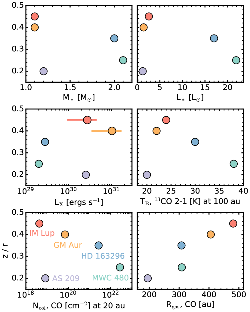
Figure 13: Average $z/r$ of ¹²CO 2–1 emission heights versus disk physical properties for the MAPS sources. Stellar masses and bolometric luminosities, taken from Oberg et al. (2021) and references therein, while X-ray luminosities references are: IM Lup (Cleeves et al., 2017), AS 209 (Walter & Kuhi, 1981), GM Aur (Espaillat et al., 2019), HD 163296 (Günther & Schmitt, 2009), and MWC 480 (Grady et al., 2010). Horizontal bars indicate observed intrinsic X-ray variability. Brightness temperatures of ¹³CO 2–1 at 100 au are interpolated directly from the T_B radial profiles in Figure 7, so they sometimes differ from the fitted $T_{100}$ in Table 2. If we instead adopted the fitted $T_{100}$ values, the conclusions are unchanged. Peak CO column densities are from Zhang et al. (2021) (and see Figure 14), while the CO 2–1 disk sizes are from Law et al. (2021).

As irradiation from the central star plays a large role in setting the shape of the emitting layers (Dullemond et al., 2001; Dullemond & Dominik, 2004a, b), we first consider whether differences in $z$/$r$ could be explain by differences in incident stellar radiation. In Figure 13, we identify a tentative negative trend between bolometric stellar luminosity and the $z/r$ of ¹²CO 2–1 emission surfaces as well as a modest positive association between X-ray luminosity and emission height. However, in both cases, AS 209 is an obvious outlier with an emission surface that is substantially flatter than the other two T Tauri sources IM Lup and GM Aur, which possess similar stellar and X-ray luminosities.

Another parameter that may set disk emitting layer heights is the temperature of the vertically isothermal layer (e.g., Qi et al., 2019). To check this, we compared the ¹³CO 2–1 gas temperatures at 100 au with emission heights in Figure 13. With the exception of AS 209, we find a negative trend, where the warmer temperatures of the two disks around the Herbig Ae stars have flatter surfaces, while the cooler temperatures of those around the T Tauri stars IM Lup and GM Aur have higher $z/r$ surfaces. We find a similar association if we instead consider the midplane temperature estimates derived from the thermo-chemical models of Zhang et al. (2021).

We next consider the physical properties of the gas itself, i.e., total disk size and column densities. We find a tight positive trend between CO 2–1 disk size and the $z/r$ of CO surfaces, as shown in Figure 13. However, the surfaces of small disks turnover at smaller radii, which may affect the $z$/$r$, but this trend remains unchanged if we instead compare using the turnover radius for each disk. Assuming that H₂ number density scales with CO column densities, we expect more dust grains in the disk upper layers due to increased dynamical gas-grain coupling. This, may in turn, manifest as higher $z$/$r$ surfaces. However, if we compare peak CO column densities, i.e., $<50$ au, versus $z$/$r$, we find an inverse relation, with AS 209 being a notable outlier to this trend. Taken together, this suggests that larger disks with lower column densities may preferentially exhibit elevated emitting surfaces.

However, these source characteristics are not all independent, since the mass of the central star either sets or influences many of them. Therefore, we also compared the stellar mass and emission surface $z/r$ in Figure 13 and found a negative trend, very similar to that of the stellar luminosity. The stellar mass sets the stellar luminosity, including the X-ray luminosity (with lower mass stars being more active), which in turn controls the disk temperature structure. Physically, warmer disks may be expected to result in increasingly flared surfaces, but this is the opposite of what we find in Figure 13. As vertical surfaces are set by the balance of pressure and gravity, disks around more massive stars should, in contrast, exhibit flatter surfaces. Since stellar mass positively correlates with disk mass (e.g., Andrews et al., 2013; Ansdell et al., 2016; Pascucci et al., 2016), this scenario is consistent with the observed trends and suggests that stellar mass is the dominant factor in setting emission surface heights. Thus, the majority of observed trends may simply be tracing the impact of varying stellar masses and the effects on the surrounding disks.

Overall, however, we caution that this small and highly biased sample of disks limits generalized conclusions. A survey aimed at targeting CO lines in a large set of moderately inclined disks with sufficient resolution and sensitivity is needed to provide further constraints on the origins and distribution of the heights of disk emitting layers.

5.3 Origins of Vertical Substructures

The emitting surfaces show several dips in vertical heights, which may have their origins in a variety of mechanisms. They may be due to CO depletion, i.e., decreased CO column density, decreases in total H₂ surface density but with constant CO abundance, or true geometrical features, e.g., warps. Here, we focus on the first two explanations and note that changes in CO abundance suggest a chemical origin, while decreases in H₂, hint at dynamical, planet-based origins.

The chemical explanation requires CO gas to be sufficiently depleted at the locations of vertical substructures. Alignments of vertical substructures with CO column density gaps, while suggestive, are not conclusive proof of a chemical origin, as gas surface density perturbations and chemical processing are often degenerate in models (e.g., Alarcón et al., 2021). However, if these features have their origins in chemistry, the depletion of gas-phase CO should lead to higher C/O ratios, causing an increase in the column density of molecules such as C₂H (Bergin et al., 2016; Alarcón et al., 2021). To test this possibility, we compare the column density profiles of CO (Zhang et al., 2021) and C₂H (Guzmán et al., 2021) with the identified vertical substructures in Figure 14. The vertical substructures Z56 in AS 209, Z46 in HD 163296, and Z66 in MWC 480 are all associated with CO column density depletions and C₂H enhancements. In contrast, Z81 and Z145 in HD 163296, as well as Z170 and Z375 in IM Lup are not. This suggests that chemical conversion of CO into other species may provide at best a partial explanation for the observed vertical substructures.

The dynamical explanation, i.e., if vertical substructures are caused by forming-planets, instead requires drops in total H₂ gas surface density. Perhaps, in this case, we expect vertical substructures to be associated with gaps in the millimeter-sized grains. As large grains should be concentrated in gas pressure maxima, this means that dust gaps will correspond to pressure minima and be associated with drops in the total H₂ gas surface density. As discussed in Section 4.4.3, all of the MAPS disks show some degree of spatial association between millimeter continuum gaps and vertical substructures. Below, we consider the plausibility of this interpretation for each MAPS disk:

In AS 209, the Z56 substructure is radially coincident with a deep gap in H₂ (Teague et al., 2018b). Moreover, Fedele et al. (2018) showed that either a single Saturn mass planet at 95 au, or a second ($<0.1~{}M_{\rm{Jup})}$ planet 57 au, reproduced the observed continuum profile. Thus, a planetary-origin for Z56 (and the larger wave-like structure) in AS 209 is possible, but c.f., Alarcón et al. (2021), who constrain the mass of a putative planet at 100 au to be ${<}0.2$ M_Jup.

In HD 163296, the derived CO surfaces, and in particular, the measured depths of vertical substructures, in HD 163296 most closely match the models of Rab et al. (2020) that include deep gas gaps, i.e., similar depletion as for the dust, at the locations of the observed millimeter continuum gaps. Similarly, the gas gap models (versus that of CO depletion) from Calahan et al. (2021) are better able to reproduce the Z81 dip in the C¹⁸O emission surface. As HD 163296 is also believed to host three Jupiter-mass planets (Pinte et al., 2018; Teague et al., 2018a), this offers a plausible explanation for the vertical substructures in this disk.

In IM Lup, GM Aur, and MWC 480, the plausibility of vertical substructures having their origins in planets is less clear. In IM Lup, Pinte et al. (2020) reported a tentative localized deviation from Keplerian rotation at 117 au, which is thought to be due to a planetary perturber. Intriguingly, this is at the same radius where we observe a change in the slope of the CO 2–1 emitting surface. GM Aur has been suggested to have a 0.1–0.4 M_Jup planet at 67 au based on the width of the nearby dust gap (Huang et al., 2020), but no vertical substructures are observed near this radius. The wave-like feature in MWC 480 shows broad associations with dust gaps, and Teague et al. (2021) propose a planet at 245 au, which is driving the wave-like perturbations.

Regardless of the specific mechanisms responsible for these vertical substructures, the MAPS data suggest that emitting surfaces are far from smooth. The locations, depths, and widths of such features provide important inputs to disk thermo-chemical models and serve as powerful probes of the planet formation. As such, they may also offer another promising mechanism to infer the existence of embedded, newly-forming planets in disks.

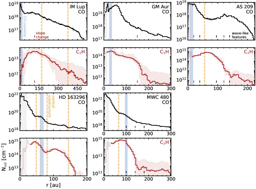
Figure 14: Column density profiles for CO (Zhang et al., 2021) and C₂H (Guzmán et al., 2021) for all MAPS sources versus locations of vertical substructures in CO, ¹³CO, and C¹⁸O 2–1 emission lines. Orange dashed lines indicates vertical dips listed in Table 4. The CO snowlines from Zhang et al. (2021) are shaded in blue. Red solid lines indicate the radial locations of changes in emission surface slope. The low-amplitude, wave-like features in AS 209 and MWC 480 are shown in black with dashed and solid lines marking troughs and peaks, respectively.

6 Conclusions

We present a detailed analysis of the vertical distribution of molecules and their emitting surfaces in high angular resolution observations in five protoplanetary disks from MAPS. We conclude the following:

1. CO emission traces the most elevated regions $z/r>0.3$, while the less abundant ¹³CO and C¹⁸O probe deeper into the disk $z/r\approx 0.1$–$0.2$. These heights correspond to approximately 3 and 1 scale heights, respectively.

2. In the disks around the T Tauri star AS 209 and Herbig Ae stars HD 163296 and MWC 480, C₂H and HCN emission heights are also measurable and they emit from $z/r\lesssim 0.1$, a region relatively close to the planet-forming disk midplane.

3. The NIR surfaces, which trace micron-sized dust, of HD 163296 and IM Lup, are lower than the CO 2–1 emission surface and lie at or slightly above that of ¹³CO 2–1.

4. We derive radial temperature distributions for all CO isotopologues and use them to estimate full 2D, ($r$, $z$) empirical temperature models for each disk.

5. Emission surfaces present substructures in the form of vertical dips, often seen in more than one CO isotopologue, and are detected in a majority of MAPS disks.

6. The wide range of vertical emission heights across the sample indicates a diversity in thermal, density, or CO abundance structures. Tentative trends suggest that star+disk systems with lower stellar masses and luminosities, as well as larger CO disk sizes exhibit the most elevated CO line-emitting surfaces. However, a larger sample of disks with well-constrained disk emitting layers is required to better understand what sets emitting layer heights in disks.

7. At least some, and possibly the majority, of vertical disk substructures have their origins in local H₂ surface density drops due to embedded planets. Others may have their origin in chemical effects, namely local reductions in CO abundance and thus CO optical depth.

Overall, we have shown an effective method for extracting the emitting layers for a sample of disks and emission lines. As disks are highly structured both radially and vertically, emission surfaces in a set of lines with varying optical depths, e.g., CO isotopologues, provide direct observational constraints on the overall 2D disk structure. Moreover, these surfaces serve as critical inputs to thermo-chemical models of disks, which are necessary to not only understand the true origins of vertical gas structures but also to connect observed molecular emission to midplane abundances, and therefore the chemical environment within which planets form.

7 Value-Added Data Products

The MAPS Value-Added Data Products described in this work can be accessed through the ALMA Archive via https://almascience.nrao.edu/alma-data/lp/maps. An interactive browser for this repository is also available on the MAPS project homepage at http://www.alma-maps.info.

For each combination of data processing (individual measurements, radially-binned, and moving average), the following data products are available:

• Emission surfaces

• Gas temperature structures, radial and full 2D ($r$, $z$) profiles

• Python script to generate the data products

Each of these VADPs are provided for CO 2–1, ¹³CO 2–1, and when available, C¹⁸O 2–1 in all MAPS disks, and for C₂H 3–2 and HCN 3–2 in HD 163296. The naming scheme for these VADPs is as follows: [disk]_[line]_[frequency]_[resolution]_[datatype], where datatype is: “individual measurements,” “radially-binned,” or “moving average.” Additional data products associated with the MAPS Large Program, including line image cubes (see Section 9, Czekala et al., 2021) and radial profiles and moment maps (see Section 7, Law et al., 2021), are also available.

Appendix A Surface Filtering and Extraction

In this section, we describe in detail the functionality of disksurf and how we used it to extract emission surfaces from line image cubes:

Before extracting surfaces, we applied the following two data filtering steps. First, a radially-varying clip was used to remove pixels that are not related to the peak of the line. This was done by calculating an azimuthally-averaged profile of the peak surface brightness and then clipping values that are more than 1$\sigma$ away. This clip threshold was increased to 2$\sigma$ for lower SNR lines, e.g., C₂H 3–2 and HCN 3–2. Then, we performed a 1D smoothing to better define the peaks using a Gaussian kernel with a full-width at half-maximum (FWHM) equal to half of the beam major axis FWHM. These two steps were found to significantly improve the ability of the code to identify the emission peaks and minimize contamination from background thermal noise.

We used the get_emission_surface function to extract the deprojected radius $r$, emission height $z$, surface brightness I_ν, and channel velocity $v$ for each pixel associated with the emitting surface. This requires knowledge of the disk inclination and position angle in order to correctly account for the deprojection. We adopted these values from Table 1 in Oberg et al. (2021) with disk inclinations ranging from 37.0^∘ (AS 209) to 53.2^∘ (GM Aur).

We then applied additional clipping based on our priors of disk physical structure. In particular, we removed extremely high $z/r$ values and large negative $z$ values, as the emission must arise from at least the midplane. We allowed points with a small negative $z$ value, i.e., $z/r>-$0.1, to remain to avoid positively biasing our averages to non-zero $z$ values. We also filtered those points with low surface brightness (less than 5 times the image cube RMS) to ensure that noise did not significantly bias the derived surfaces. However, due to the lower SNR of the C₂H and HCN lines, we did not perform this clipping in any disk except for HD 163296. Figure 15 shows an example of this process for CO 2–1 in IM Lup.

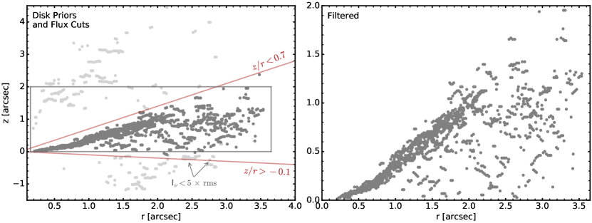
Figure 15: Clipping based on disk priors and flux (left) and filtered emission surfaces (right) for CO 2–1 in IM Lup. The gray box in the left panel shows the field of view in the right panel. Light gray points are filtered according to the steps described in detail in Appendix A.

Appendix B Full list of isovelocity contours

Isovelocity contours for the CO isotopologues are shown for the IM Lup disk in Figure 16. A full set of isovelocity contours for all MAPS disks are shown in Figure Set 1, which is available in the electronic edition of the journal. All isovelocity contours are calculated using updated dynamical masses taken from Oberg et al. (2021), which are based on CO rotation profiles (Teague et al., 2021).

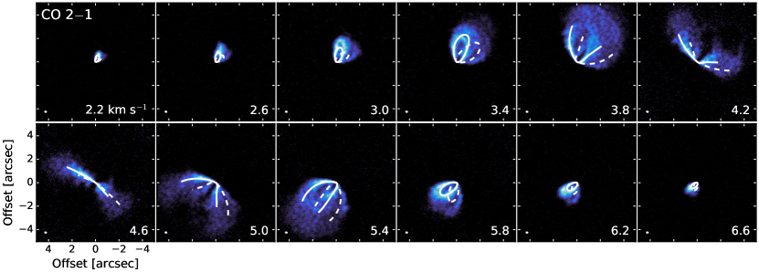
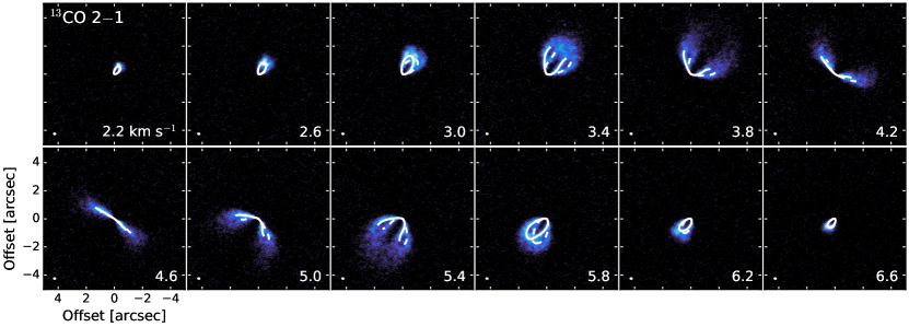
Figure 16: Isovelocity contours of the best-fitting model, as indicated in Table 1, for the CO 2–1 (top) and ¹³CO 2–1 (bottom) emitting surfaces in IM Lup plotted for selected channels of the observed emission. Solid curves indicate the upper surface of the disk and dashed curves mark the lower surface. LSRK velocities are noted in the lower right corner. The synthesized beam is shown in the bottom left corner of each panel.

Appendix C Excitation and Band 3 CO Surfaces

Since we also had access to ¹³CO 1–0, we were able to compare against the ¹³CO 2–1 line to see if we could identify any excitation-related effects in the emission surfaces, i.e., differing heights (e.g., van Zadelhoff et al., 2001; Dartois et al., 2003). Due to the coarser spatial resolution and lower SNR of the 1–0 line, we did not attempt to extract the emission surfaces directly. Instead, we compared the ¹³CO 2–1 isovelocity contours derived from the parametric fit in Table 1 with the spatial distribution of the 1–0 line. To ensure a consistent comparison, we also included the tapered (0$\farcs$30) resolution ¹³CO 2–1 images. We checked C¹⁸O 1–0, which was also covered by the MAPS observations, but it did not possess sufficient SNR for this comparison, so we instead focused on ¹³CO 1–0. At this lower resolution, only GM Aur, HD 163296, and IM Lup had sufficiently elevated ¹³CO 2–1 surfaces to allow for a meaningful comparison.

Figure 17 shows isovelocity contours overlaid on a representative channel of ¹³CO 1–0 emission that should best show the emitting layers, if resolved. In IM Lup and GM Aur, line emission tracing the back side of the disks is visible in the tapered 2–1 image, but we cannot determine if the contours are consistent with low SNR emission surfaces in ¹³CO 1–0, or if the 1–0 line is truly flatter than the 2–1 line. In the case of HD 163296, the spatial resolution is insufficient to reveal any vertical disk structure in either the ¹³CO 2–1 tapered or 1–0 images, and we therefore cannot compare 2-1 and 1-0 emission layer heights. Thus, in order to infer the emitting heights of ¹³CO 1–0, we likely require both higher spatial resolution and SNR.

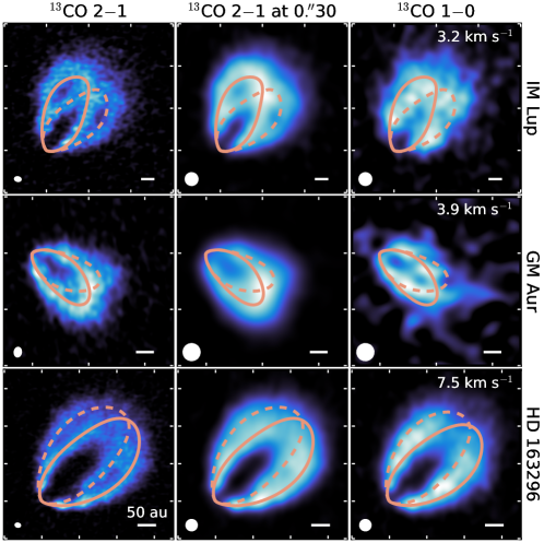
Figure 17: Representative channels for IM Lup, GM Aur, and HD 163296 for the ¹³CO 2–1 full resolution (left column), ¹³CO 2–1, tapered to 0$\farcs$30 (middle column), and ¹³CO 1–0 (right column) images. The ¹³CO 2–1 isovelocity contours derived using the parametric fit in Table 1 are shown in pink. Solid curves indicate the upper surface of the disk and dashed curves mark the lower surface. LSRK velocities are noted in the upper right corner. The synthesized beam and a scale bar indicating 50 au is shown in the lower left and right corner, respectively, of each panel.

Appendix D Effects of spatial resolution on derived emission surfaces

To extract emission surfaces using disksurf, the imagecubes must have some minimum angular resolution, i.e., the front and back sides of the disk must be sufficiently spatially resolved to be separable. This means that emission surfaces will be sensitive to the spatial resolution of the images used to derive them. To investigate the effects of spatial resolution on our surfaces, we repeated the surface extraction for CO, ¹³CO, and C¹⁸O 2–1 using all angular resolutions, i.e., 0$\farcs$3, 0$\farcs$2, 0$\farcs$15, imaged as part of MAPS (Oberg et al., 2021). We then compared them to the surfaces derived from the images generated with a robust parameter of 0.5 used throughout this work. Figures 18, 19, and 20 show the resulting surfaces.

The CO isotopologue surfaces are generally consistent across differing spatial resolutions. The lower resolutions (0$\farcs$3, 0$\farcs$2) occasionally underestimate the average $z/r$ surface height, e.g., ¹³CO and C¹⁸O in HD 163296, and this effect is more conspicuous in intrinsically flatter surfaces, e.g., ¹³CO and C¹⁸O in MWC 480 or those from rarer isotopologues. In highly-elevated surfaces like ¹²CO 2–1, the emission structure along a given column of pixels will be two well-separated Gaussians (and another two Gaussians for the backside of the disk). At lower spatial resolutions, these Gaussians are broadened, but do not overlap. Conversely, for ¹³CO or other emission lines with lower intrinsic $z/r$, these two components may overlap and thus lead to a single-peaked Gaussian with a $z/r$ that approaches 0. Even for those highly flared surfaces, images with higher spatial resolutions are preferable, as they allow for the detection and characterization of vertical substructures, such as the dips, wave-like features, and slope changes seen in many of the MAPS disks (see Section 4.4). For instance, the ¹²CO surface in HD 163296 appears nearly identical between the 0$\farcs$3 and robust=0.5 images, with the important exception of the Z46 dip, which can only identified in the 0$\farcs$15 and robust=0.5 images.

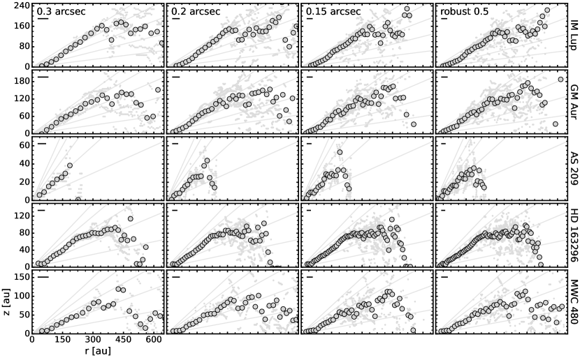
Figure 18: ¹²CO 2–1 emission surfaces derived using images with different angular resolutions (see Table 5 in Oberg et al. 2021). Large, gray points show a consistent radial binning of 1/2$\times$ the beam major axis of each image, while small, light gray points represent individual measurements. Lines of constant $z/r$ from 0.1 to 0.5 in increments of 0.1 are shown in gray. The FWHM of the major axis of the synthesized beam is shown in the upper left corner of each panel.

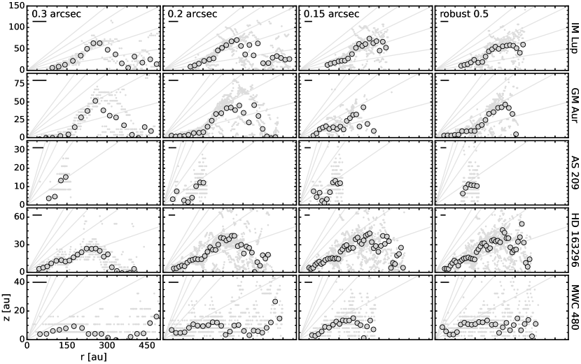
Figure 19: ¹³CO 2–1 emission surfaces derived using different spatial resolutions. Otherwise, as in Figure 18.

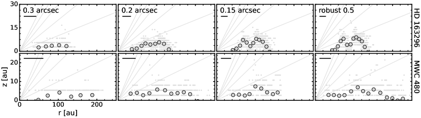
Figure 20: C¹⁸O 2–1 emission surfaces derived using different spatial resolutions for HD 163296 and MWC 480. The C¹⁸O 2–1 surface in GM Aur is not shown as it was only able to be extracted from the images generated with a robust parameter of 0.5, as only this image possessed a sufficiently high spatial resolution necessary to separate the front and back disk surfaces. Otherwise, as in Figure 18.

References

- Alarcón et al. (2021) Alarcón, F., Bosman, A., Bergin, E., et al. 2021, arXiv e-prints, arXiv:2109.06263. https://arxiv.org/abs/2109.06263
- Andrews (2020) Andrews, S. M. 2020, ARA&A, 58, 483, doi: 10.1146/annurev-astro-031220-010302
- Andrews et al. (2013) Andrews, S. M., Rosenfeld, K. A., Kraus, A. L., & Wilner, D. J. 2013, ApJ, 771, 129, doi: 10.1088/0004-637X/771/2/129
- Andrews et al. (2018) Andrews, S. M., Huang, J., Pérez, L. M., et al. 2018, ApJ, 869, L41, doi: 10.3847/2041-8213/aaf741
- Ansdell et al. (2016) Ansdell, M., Williams, J. P., van der Marel, N., et al. 2016, ApJ, 828, 46, doi: 10.3847/0004-637X/828/1/46
- Astropy Collaboration et al. (2013) Astropy Collaboration, Robitaille, T. P., Tollerud, E. J., et al. 2013, A&A, 558, A33, doi: 10.1051/0004-6361/201322068
- Avenhaus et al. (2018) Avenhaus, H., Quanz, S. P., Garufi, A., et al. 2018, ApJ, 863, 44, doi: 10.3847/1538-4357/aab846
- Bergin et al. (2016) Bergin, E. A., Du, F., Cleeves, L. I., et al. 2016, ApJ, 831, 101, doi: 10.3847/0004-637X/831/1/101
- Boehler et al. (2017) Boehler, Y., Weaver, E., Isella, A., et al. 2017, ApJ, 840, 60, doi: 10.3847/1538-4357/aa696c
- Bosman et al. (2021) Bosman, A. D., Bergin, E. A., Loomis, R. A., et al. 2021, arXiv e-prints, arXiv:2109.06223. https://arxiv.org/abs/2109.06223
- Calahan et al. (2021) Calahan, J. K., Bergin, E. A., Zhang, K., et al. 2021, arXiv e-prints, arXiv:2109.06202. https://arxiv.org/abs/2109.06202
- Cleeves (2016) Cleeves, L. I. 2016, ApJ, 816, L21, doi: 10.3847/2041-8205/816/2/L21
- Cleeves et al. (2017) Cleeves, L. I., Bergin, E. A., Öberg, K. I., et al. 2017, ApJ, 843, L3, doi: 10.3847/2041-8213/aa76e2
- Cleeves et al. (2016) Cleeves, L. I., Öberg, K. I., Wilner, D. J., et al. 2016, ApJ, 832, 110, doi: 10.3847/0004-637X/832/2/110
- Cleeves et al. (2021) Cleeves, L. I., Loomis, R. A., Teague, R., et al. 2021, ApJ, 911, 29, doi: 10.3847/1538-4357/abe862
- Czekala et al. (2021) Czekala, I., Loomis, R. A., Teague, R., et al. 2021, arXiv e-prints, arXiv:2109.06188. https://arxiv.org/abs/2109.06188
- Dartois et al. (2003) Dartois, E., Dutrey, A., & Guilloteau, S. 2003, A&A, 399, 773, doi: 10.1051/0004-6361:20021638
- de Gregorio-Monsalvo et al. (2013) de Gregorio-Monsalvo, I., Ménard, F., Dent, W., et al. 2013, A&A, 557, A133, doi: 10.1051/0004-6361/201321603
- Dong et al. (2019) Dong, R., Liu, S.-Y., & Fung, J. 2019, ApJ, 870, 72, doi: 10.3847/1538-4357/aaf38e
- Dullemond & Dominik (2004a) Dullemond, C. P., & Dominik, C. 2004a, A&A, 417, 159, doi: 10.1051/0004-6361:20031768
- Dullemond & Dominik (2004b) —. 2004b, A&A, 421, 1075, doi: 10.1051/0004-6361:20040284
- Dullemond et al. (2001) Dullemond, C. P., Dominik, C., & Natta, A. 2001, ApJ, 560, 957, doi: 10.1086/323057
- Dullemond et al. (2020) Dullemond, C. P., Isella, A., Andrews, S. M., Skobleva, I., & Dzyurkevich, N. 2020, A&A, 633, A137, doi: 10.1051/0004-6361/201936438
- Dutrey et al. (2017) Dutrey, A., Guilloteau, S., Piétu, V., et al. 2017, A&A, 607, A130, doi: 10.1051/0004-6361/201730645
- Espaillat et al. (2019) Espaillat, C. C., Robinson, C., Grant, S., & Reynolds, M. 2019, ApJ, 876, 121, doi: 10.3847/1538-4357/ab16e6
- Facchini et al. (2017) Facchini, S., Birnstiel, T., Bruderer, S., & van Dishoeck, E. F. 2017, A&A, 605, A16, doi: 10.1051/0004-6361/201630329
- Favre et al. (2019) Favre, C., Fedele, D., Maud, L., et al. 2019, ApJ, 871, 107, doi: 10.3847/1538-4357/aaf80c
- Fedele et al. (2018) Fedele, D., Tazzari, M., Booth, R., et al. 2018, A&A, 610, A24, doi: 10.1051/0004-6361/201731978
- Fogel et al. (2011) Fogel, J. K. J., Bethell, T. J., Bergin, E. A., Calvet, N., & Semenov, D. 2011, ApJ, 726, 29, doi: 10.1088/0004-637X/726/1/29
- Foreman-Mackey et al. (2013) Foreman-Mackey, D., Hogg, D. W., Lang, D., & Goodman, J. 2013, PASP, 125, 306, doi: 10.1086/670067
- Goodman & Weare (2010) Goodman, J., & Weare, J. 2010, Communications in Applied Mathematics and Computational Science, 5, 65, doi: 10.2140/camcos.2010.5.65
- Grady et al. (2010) Grady, C. A., Hamaguchi, K., Schneider, G., et al. 2010, ApJ, 719, 1565, doi: 10.1088/0004-637X/719/2/1565
- Günther & Schmitt (2009) Günther, H. M., & Schmitt, J. H. M. M. 2009, A&A, 494, 1041, doi: 10.1051/0004-6361:200811007
- Guzmán et al. (2018) Guzmán, V. V., Öberg, K. I., Carpenter, J., et al. 2018, ApJ, 864, 170, doi: 10.3847/1538-4357/aad778
- Guzmán et al. (2021) Guzmán, V. V., Bergner, J. B., Law, C. J., et al. 2021, arXiv e-prints, arXiv:2109.06391. https://arxiv.org/abs/2109.06391
- Huang et al. (2018) Huang, J., Andrews, S. M., Dullemond, C. P., et al. 2018, ApJ, 869, L42, doi: 10.3847/2041-8213/aaf740
- Huang et al. (2020) —. 2020, ApJ, 891, 48, doi: 10.3847/1538-4357/ab711e
- Hunter (2007) Hunter, J. D. 2007, Computing in Science and Engineering, 9, 90, doi: 10.1109/MCSE.2007.55
- Ilgner et al. (2004) Ilgner, M., Henning, T., Markwick, A. J., & Millar, T. J. 2004, A&A, 415, 643, doi: 10.1051/0004-6361:20034061
- Isella et al. (2018) Isella, A., Huang, J., Andrews, S. M., et al. 2018, ApJ, 869, L49, doi: 10.3847/2041-8213/aaf747
- Kenyon & Hartmann (1987) Kenyon, S. J., & Hartmann, L. 1987, ApJ, 323, 714, doi: 10.1086/165866
- Kusakabe et al. (2012) Kusakabe, N., Grady, C. A., Sitko, M. L., et al. 2012, ApJ, 753, 153, doi: 10.1088/0004-637X/753/2/153
- Law et al. (2021) Law, C. J., Loomis, R. A., Teague, R., et al. 2021, arXiv e-prints, arXiv:2109.06210. https://arxiv.org/abs/2109.06210
- McMullin et al. (2007) McMullin, J. P., Waters, B., Schiebel, D., Young, W., & Golap, K. 2007, in Astronomical Society of the Pacific Conference Series, Vol. 376, Astronomical Data Analysis Software and Systems XVI, ed. R. A. Shaw, F. Hill, & D. J. Bell, 127
- Monnier et al. (2017) Monnier, J. D., Harries, T. J., Aarnio, A., et al. 2017, ApJ, 838, 20, doi: 10.3847/1538-4357/aa6248
- Morbidelli et al. (2014) Morbidelli, A., Szulágyi, J., Crida, A., et al. 2014, Icarus, 232, 266, doi: 10.1016/j.icarus.2014.01.010
- Muro-Arena et al. (2018) Muro-Arena, G. A., Dominik, C., Waters, L. B. F. M., et al. 2018, A&A, 614, A24, doi: 10.1051/0004-6361/201732299
- Öberg et al. (2011) Öberg, K. I., Qi, C., Fogel, J. K. J., et al. 2011, ApJ, 734, 98, doi: 10.1088/0004-637X/734/2/98
- Öberg et al. (2021) Öberg, K. I., Cleeves, L. I., Bergner, J. B., et al. 2021, AJ, 161, 38, doi: 10.3847/1538-3881/abc74d
- Oberg et al. (2021) Oberg, K. I., Guzman, V. V., Walsh, C., et al. 2021, arXiv e-prints, arXiv:2109.06268. https://arxiv.org/abs/2109.06268
- Paneque-Carreño et al. (2021) Paneque-Carreño, T., Pérez, L. M., Benisty, M., et al. 2021, ApJ, 914, 88, doi: 10.3847/1538-4357/abf243
- Pascucci et al. (2016) Pascucci, I., Testi, L., Herczeg, G. J., et al. 2016, ApJ, 831, 125, doi: 10.3847/0004-637X/831/2/125
- Piétu et al. (2007) Piétu, V., Dutrey, A., & Guilloteau, S. 2007, A&A, 467, 163, doi: 10.1051/0004-6361:20066537
- Pinte et al. (2018) Pinte, C., Ménard, F., Duchêne, G., et al. 2018, A&A, 609, A47, doi: 10.1051/0004-6361/201731377
- Pinte et al. (2020) Pinte, C., Price, D. J., Ménard, F., et al. 2020, ApJ, 890, L9, doi: 10.3847/2041-8213/ab6dda
- Podio et al. (2020) Podio, L., Garufi, A., Codella, C., et al. 2020, A&A, 642, L7, doi: 10.1051/0004-6361/202038952
- Price-Whelan et al. (2018) Price-Whelan, A. M., Sipőcz, B. M., Günther, H. M., et al. 2018, AJ, 156, 123, doi: 10.3847/1538-3881/aabc4f
- Qi et al. (2019) Qi, C., Öberg, K. I., Espaillat, C. C., et al. 2019, ApJ, 882, 160, doi: 10.3847/1538-4357/ab35d3
- Rab et al. (2020) Rab, C., Kamp, I., Dominik, C., et al. 2020, A&A, 642, A165, doi: 10.1051/0004-6361/202038712
- Rich et al. (2020) Rich, E. A., Wisniewski, J. P., Sitko, M. L., et al. 2020, ApJ, 902, 4, doi: 10.3847/1538-4357/abb2a3
- Rich et al. (2021) Rich, E. A., Teague, R., Monnier, J. D., et al. 2021, ApJ, 913, 138, doi: 10.3847/1538-4357/abf92e
- Rosenfeld et al. (2013) Rosenfeld, K. A., Andrews, S. M., Hughes, A. M., Wilner, D. J., & Qi, C. 2013, ApJ, 774, 16, doi: 10.1088/0004-637X/774/1/16
- Ruíz-Rodríguez et al. (2021) Ruíz-Rodríguez, D., Kastner, J., Hily-Blant, P., & Forveille, T. 2021, A&A, 646, A59, doi: 10.1051/0004-6361/202038209
- Schneider et al. (2003) Schneider, G., Wood, K., Silverstone, M. D., et al. 2003, AJ, 125, 1467, doi: 10.1086/367596
- Semenov & Wiebe (2011) Semenov, D., & Wiebe, D. 2011, ApJS, 196, 25, doi: 10.1088/0067-0049/196/2/25
- Sierra et al. (2021) Sierra, A., Pérez, L. M., Zhang, K., et al. 2021, arXiv e-prints, arXiv:2109.06433. https://arxiv.org/abs/2109.06433
- Teague (2019) Teague, R. 2019, The Journal of Open Source Software, 4, 1632, doi: 10.21105/joss.01632
- Teague et al. (2019) Teague, R., Bae, J., & Bergin, E. A. 2019, Nature, 574, 378, doi: 10.1038/s41586-019-1642-0
- Teague et al. (2018a) Teague, R., Bae, J., Bergin, E. A., Birnstiel, T., & Foreman-Mackey, D. 2018a, ApJ, 860, L12, doi: 10.3847/2041-8213/aac6d7
- Teague et al. (2018b) Teague, R., Bae, J., Birnstiel, T., & Bergin, E. A. 2018b, ApJ, 868, 113, doi: 10.3847/1538-4357/aae836
- Teague & Foreman-Mackey (2018) Teague, R., & Foreman-Mackey, D. 2018, Bettermoments: A Robust Method To Measure Line Centroids, v1.0, Zenodo, doi: 10.5281/zenodo.1419754
- Teague et al. (2020) Teague, R., Jankovic, M. R., Haworth, T. J., Qi, C., & Ilee, J. D. 2020, MNRAS, 495, 451, doi: 10.1093/mnras/staa1167
- Teague et al. (2021) Teague, R., Bae, J., Aikawa, Y., et al. 2021, arXiv e-prints, arXiv:2109.06218. https://arxiv.org/abs/2109.06218
- van der Walt et al. (2011) van der Walt, S., Colbert, S. C., & Varoquaux, G. 2011, Computing in Science and Engineering, 13, 22, doi: 10.1109/MCSE.2011.37
- van Zadelhoff et al. (2001) van Zadelhoff, G. J., van Dishoeck, E. F., Thi, W. F., & Blake, G. A. 2001, A&A, 377, 566, doi: 10.1051/0004-6361:20011137
- Virtanen et al. (2020) Virtanen, P., Gommers, R., Oliphant, T. E., et al. 2020, Nature Methods, doi: https://doi.org/10.1038/s41592-019-0686-2
- Walsh et al. (2010) Walsh, C., Millar, T. J., & Nomura, H. 2010, ApJ, 722, 1607, doi: 10.1088/0004-637X/722/2/1607
- Walter & Kuhi (1981) Walter, F. M., & Kuhi, L. V. 1981, ApJ, 250, 254, doi: 10.1086/159370
- Weaver et al. (2018) Weaver, E., Isella, A., & Boehler, Y. 2018, ApJ, 853, 113, doi: 10.3847/1538-4357/aaa481
- Williams & Cieza (2011) Williams, J. P., & Cieza, L. A. 2011, ARA&A, 49, 67, doi: 10.1146/annurev-astro-081710-102548
- Woitke et al. (2009) Woitke, P., Kamp, I., & Thi, W. F. 2009, A&A, 501, 383, doi: 10.1051/0004-6361/200911821
- Zhang et al. (2021) Zhang, K., Booth, A. S., Law, C. J., et al. 2021, arXiv e-prints, arXiv:2109.06233. https://arxiv.org/abs/2109.06233
- Zhu et al. (2019) Zhu, Z., Zhang, S., Jiang, Y.-F., et al. 2019, ApJ, 877, L18, doi: 10.3847/2041-8213/ab1f8c