Molecules with ALMA at Planet-forming Scales (MAPS) III: Characteristics of Radial Chemical Substructures

Abstract

The Molecules with ALMA at Planet-forming Scales (MAPS) Large Program provides a detailed, high resolution (${\sim}$10–20 au) view of molecular line emission in five protoplanetary disks at spatial scales relevant for planet formation. Here, we present a systematic analysis of chemical substructures in 18 molecular lines toward the MAPS sources: IM Lup, GM Aur, AS 209, HD 163296, and MWC 480. We identify more than 200 chemical substructures, which are found at nearly all radii where line emission is detected. A wide diversity of radial morphologies — including rings, gaps, and plateaus — is observed both within each disk and across the MAPS sample. This diversity in line emission profiles is also present in the innermost 50 au. Overall, this suggests that planets form in varied chemical environments both across disks and at different radii within the same disk. Interior to 150 au, the majority of chemical substructures across the MAPS disks are spatially coincident with substructures in the millimeter continuum, indicative of physical and chemical links between the disk midplane and warm, elevated molecular emission layers. Some chemical substructures in the inner disk and most chemical substructures exterior to 150 au cannot be directly linked to dust substructure, however, which indicates that there are also other causes of chemical substructures, such as snowlines, gradients in UV photon fluxes, ionization, and radially-varying elemental ratios. This implies that chemical substructures could be developed into powerful probes of different disk characteristics, in addition to influencing the environments within which planets assemble. This paper is part of the MAPS special issue of the Astrophysical Journal Supplement.

1 Introduction

Protoplanetary disks provide the constituent materials necessary for forming planets. The colliding and coalescing of dust grains leads to the formation of pebbles, which grow into planetesimals and ultimately planets (e.g., Mordasini et al., 2008), while the spatial distribution of ice and gas sets the volatile compositions of incipient planets (Öberg et al., 2011a). The diversity of known exoplanetary systems (e.g., Batalha et al., 2013) may originate, at least in part, due to differences in the gas and dust distribution observed across protoplanetary disks (e.g., Mordasini et al., 2012). Disk observations can thus provide crucial constraints on the formation locations of planets (Zhu et al., 2014; Zhang et al., 2018) and the processes by which initial gas and dust distributions evolve into planetary systems (Birnstiel et al., 2015; van der Marel et al., 2015; Pérez et al., 2015; Andrews, 2020). Moreover, the organic compositions of planets are linked to the chemistry of their parental disks (Öberg & Bergin, 2016; Cridland et al., 2016, 2017), which makes a detailed understanding of the chemical environment in which young planets form of particular interest to origins of life studies.

Disk chemistry is regulated by a combination of inherited material and in situ processes that depend on density, temperature, and radiation fields. While models of chemical structures often assume smoothly-decreasing surface densities and temperatures (Hughes et al., 2008; Andrews et al., 2009), disks are now known to be highly-structured in their dust (ALMA Partnership et al., 2015; Andrews et al., 2016; Long et al., 2018a) and gas (Isella et al., 2016a; Teague et al., 2017; Huang et al., 2018a). The DSHARP program (Huang et al., 2018b; Andrews et al., 2018), and subsequent observations (e.g., Facchini et al., 2020; Cieza et al., 2021), showed that dust substructures at 1-to-10 au scales in the form of rings, gaps, and spirals are ubiquitous in protoplanetary disks. Disks also possess complex gas distributions and exhibit gradients in C/N/O ratios and organic molecules (e.g., Bergin et al., 2016; Cleeves, 2016; Isella et al., 2016b; van der Marel et al., 2016; Huang et al., 2017; Bergner et al., 2018; Huang et al., 2018a; Kastner et al., 2018; Bergner et al., 2019; Garufi et al., 2020; Pegues et al., 2020; Facchini et al., 2021; Booth et al., 2021). However, the majority of molecular line observations have been limited to coarser angular resolutions (${\sim}$0$\farcs$5–1$\farcs$0), which trace physical scales of 50–150 au at typical distances (${\sim}$100–150 pc) of nearby disks (e.g., Dartois et al., 2003; Piétu et al., 2007; Chapillon et al., 2012; Mathews et al., 2013; de Gregorio-Monsalvo et al., 2013; Flaherty et al., 2017; Salinas et al., 2017; Le Gal et al., 2019b). The relatively small number of studies at high spatial resolutions (${<}$0$\farcs$3) have focused on CO (Fedele et al., 2017; Pinte et al., 2018; Isella et al., 2018; Favre et al., 2019; Rosotti et al., 2020; Wölfer et al., 2021), and perhaps one or two additional molecules such as C₂H (Bergin et al., 2016; Miotello et al., 2019), CN (van Terwisga et al., 2019; Teague & Loomis, 2020a), HCO⁺ (Long et al., 2018b; Tsukagoshi et al., 2019; Huang et al., 2020), H₂CO (Podio et al., 2019), and CS (Rosotti et al., 2021; Nomura et al., 2021). Thus, the detailed structure of the gas component of disks remains largely unexplored, especially toward the inner, planet-forming regions (${<}100$ au).

Hence, the relationship between chemical and dust structure at small scales is unclear. As the distribution of dust strongly impacts the chemistry (Cleeves, 2016; Facchini et al., 2017; van der Marel et al., 2018), it is expected that the presence of dust substructures will also alter local chemical environments. This is because the total surface area of dust present throughout the disk is linked to many physical and chemical processes, such as the disk thermal structure, thermal coupling between the gas and solid phases, and balance between freeze-out and desorption. Additionally, grain growth and vertical settling affect the penetration depth of UV photons, which in turn alters the chemistry and gas temperatures (e.g., Fogel et al., 2011; Akimkin et al., 2013; Cleeves, 2016).

A systematic analysis of a wide set of molecular lines is required in order to assess the relationship between chemical and dust substructures in disks and establish a clearer understanding of the chemical environments in which planets form. To this end, we quantitatively characterize the properties of chemical substructures observed as part of the Molecules with ALMA at Planet-forming Scales (MAPS) Large Program (Oberg et al., 2021). In Section 2, we discuss the generation of moment maps and radial profiles. In Section 3, we describe how we measured the locations, widths, and relative contrasts of the observed chemical substructures. We present aggregate properties of substructures in Section 4 and examine spatial trends in their locations and discuss possible origins in Section 5. We summarize our findings in Section 6 and provide a listing of all available data products in Section 7.

2 Generation of Moment Maps and Radial Profiles

2.1 Observations

The MAPS Large Program (2018.1.01055.L) targeted the protoplanetary disks around IM Lup, GM Aur, AS 209, HD 163296, and MWC 480 in four spectral setups in ALMA Bands 6 and 3. Figure 1 shows an overview of each disk in CO $2-1$ and continuum emission. The analysis presented here is based on the fiducial images, as described in Oberg et al. (2021), which have 0$\farcs$15 and 0$\farcs$30 circularized beams for lines in Bands 6 and 3, respectively. For those transitions covered in Band 6 that were either marginally detected or lacked sufficient signal-to-noise ratio (SNR), we instead used the corresponding tapered (0$\farcs$30) images (see Section 6.2, Czekala et al., 2021). The correction for a significantly non-Gaussian dirty beam, i.e., the “JvM correction” first described in Jorsater & van Moorsel (1995), is salient to the following discussion and is explained in detail in Czekala et al. (2021), together with the full imaging procedure. Briefly, the application of the “JvM-correction” correctly scales the residuals in the image cube to be in units consistent with the CLEAN model. This ensures that the starting point for the moment map generation, the CLEANed image, is in the correct units of Jy {$\mathrm{CLEAN\,beam}^{-1}$}. Oberg et al. (2021) provides details about the observational setup and calibration, as well as basic information about each image, including the JvM-corrected RMS noise level.

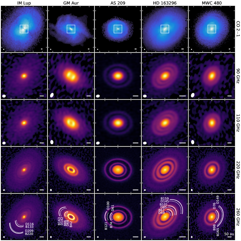
Figure 1: Zeroth moment maps of CO 2$-$1 and continuum images for the MAPS sample, ordered from left to right by increasing stellar mass (see Table 1 in Oberg et al. (2021)). Axes are angular offsets from the disk center and the white rectangle overlaid on the CO 2$-$1 zeroth moment maps defines the field of view of the continuum images. Each tick mark is 2^′′ and 1^′′ for the CO 2$-$1 and continuum images, respectively. Color stretches were individually optimized and applied to each panel to increase the visibility of substructures. Care should thus be taken when comparing between panels, and instead, we recommend using the corresponding radial profiles in Figure 14 for this purpose. Continuum substructures, as described in Section 3.4, are labeled on the 260 GHz continuum images following the nomenclature of Huang et al. (2018b). Rings and gaps are shown as solid and dotted arcs, respectively, with azimuthal extents chosen for maximal visual clarity. The synthesized beam and a scale bar indicating 50 au is shown in the lower left and right corner, respectively, of each panel.

We focus this work on 18 lines, listed in Table 1, that are sufficiently bright and spatially extended to allow for an analysis of radial substructures. We analyzed only the brightest component of those transitions with multiple hyperfine components, namely C₂H N=3–2, J=$\frac{7}{2}$–$\frac{5}{2}$, F=4–3; C₂H N=1–0, J=$\frac{3}{2}$–$\frac{1}{2}$, F=2–1; c-C₃H₂ (J${}_{\rm{K}_{\rm{a}},{\rm{K}_{\rm{c}}}}$)=7₀₇–6₁₆/7₁₇–6₀₆, HCN J=3–2, F=3–2; and HCN J=1–0, F=2–1. Subsequently, we refer to these lines as C₂H 3–2, 1–0; c-C₃H₂ 7–6; and HCN 3–2, 1–0. Due to difficulties in separating the closely-spaced F=$\frac{3}{2}$–$\frac{1}{2}$ and F=$\frac{5}{2}$–$\frac{3}{2}$ hyperfine lines of the CN N=1–0, J=$\frac{3}{2}$–$\frac{1}{2}$ transition, we instead combined them to increase the SNR and improve radial substructure identification. From now on, we refer to these combined lines as CN 1$-$0. Additional details about the CN lines are in Bergner et al. (2021). We also combined the blended CH₃CN J=12$-$11, K=0 and K=1 lines (see Ilee et al., 2021), which we simply designate as CH₃CN 12$-$11 for the remainder of this work. For simplicity, we likewise label the H₂CO (J${}_{\rm{K}_{\rm{a}},{\rm{K}_{\rm{c}}}}$)=3${}_{03}-$2₀₂ line as H₂CO 3$-$2. A comprehensive set of observed transitions is presented in Oberg et al. (2021), and detailed analyses of weaker and less spatially extended lines not discussed here can be found in Aikawa et al. (2021); Cataldi et al. (2021); Ilee et al. (2021); Le Gal et al. (2021); Zhang et al. (2021).

In the following subsections, we describe the creation of a set of publicly available Value-Added Data Products (VADPs), namely moment maps and radial intensity profiles. Although line image cubes in principle contain maximal information, the creation of such products is necessary to reduce the overall dimensionality and more intuitively visualize and interpret the data.

2.2 Moment maps

A map of the velocity-integrated intensity, or “zeroth moment map,” is often useful as a summary representation of an image cube. In this subsection, we describe the process by which we generate moment maps and describe the non-uniform noise distribution that frequently occurs in protoplanetary disk applications.

In its simplest form, a moment map is generated by collapsing an image cube along the velocity dimension to produce a two-dimensional representation of the velocity-integrated flux. Whereas image cubes have units of $\mathrm{Jy\,beam}^{-1}$, moment maps have units of $\mathrm{Jy\,beam}^{-1}\,\mathrm{km\,s}^{-1}$. For sources with complex position-position-velocity morphologies, it is common to first apply a mask to the image cube, so as to prevent regions known to be free of source emission from contributing noise to the moment map.

We adopted a Keplerian mask identical to the one used during the CLEANing process (for more details, see Czekala et al. (2021)). We did not use a flux threshold for pixel inclusion, i.e., sigma clipping, to ensure accurate flux recovery. We used the Python package bettermoments (Teague & Foreman-Mackey, 2018) to generate zeroth moment maps from the non-primary-beam corrected image cubes.

While the use of a mask can substantially improve the visual appearance of a moment map, as shown in Teague (2019a), it can also introduce strong spatial variance in the noise distribution. As an example, Figure 2 shows the number of unmasked channels that were summed to create the zeroth moment map for ¹³CO 2–1 in HD 163296. Assuming that each channel in the image cube is independent and has the same noise distribution, the noise in the moment map grows $\propto\sqrt{N}$, where $N$ is the number of channels summed. On the other hand, the signal in the moment map will not necessarily grow with $\propto N$, because the sky brightness is not uniform across the image cube.

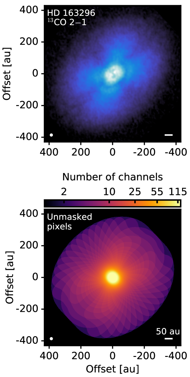
Figure 2: Zeroth moment map (top) of ¹³CO 2–1 in HD 163296 and a map of unmasked pixels (bottom) used in its generation. The colorscale shows the number of unmasked channels that were summed to create the zeroth moment map. A log10 color stretch has been applied to highlight those disk regions at larger radii with comparatively fewer summed channels. Spatial discontinuities from the Keplerian masking process are evident.

The discontinuous noise distribution created by the Keplerian masks occasionally imprinted arc-like artifacts in the central few arcseconds of zeroth moment maps created from weak and moderately-bright line image cubes. Such artifacts are the result of channelization and have no effect on the flux properties of the final moment maps, so long as the uncertainties are correctly accounted for. All subsequent quantitative analysis, including the generation of radial intensity profiles, was done using these unclipped and Keplerian masked zeroth moment maps.

While quantitatively correct, unclipped zeroth moment maps may sometimes be visually misleading due to similarities between arc-like artifacts and real substructures. To address this, we also generated a set of “hybrid” zeroth moment maps using an approach similar to the auto-masking routine employed within CASA (Kepley et al., 2020). This combines Keplerian CLEAN masks with smoothed intensity-based masks, which is described in more detail in Appendix A. These hybrid maps mitigate or remove the majority of these artifacts and thus better visualize radial structures compared to the zeroth moment maps generated directly from the Keplerian masks. Figures 3, 4, 5, and 6 show these hybrid zeroth moment maps on a line-by-line basis, while source-specific galleries are found in Appendix B. As the sigma clipping used to generate these hybrid zeroth moment maps artificially reduces integrated intensities, we emphasize these maps are only presentational in nature and are never used for quantitative analysis.

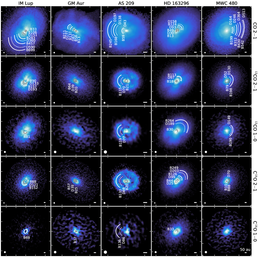
Figure 3: Zeroth moment maps of CO, ¹³CO, and C¹⁸O lines for the MAPS sample, ordered from left to right by increasing stellar mass (see Table 1 in Oberg et al. (2021)). Axes are angular offsets from the disk center with each white tick mark represents a spacing of 2^′′. Color stretches were individually optimized and applied to each panel to increase the visibility of substructures. Care should thus be taken when comparing between panels, and instead, we recommend using the corresponding radial profiles in Figure 9 for this purpose. Chemical substructures from Table 3 in the form of rings and gaps are marked by solid and dotted arcs, respectively, with azimuthal extents and colors chosen for maximal visual clarity. Several inner low-contrast CO 2–1 substructures in IM Lup (D50, B68, D80) and HD 163296 (D71, B81) are omitted for visual clarity. The synthesized beam and a scale bar indicating 50 au is shown in the lower left and right corner, respectively, of each panel.

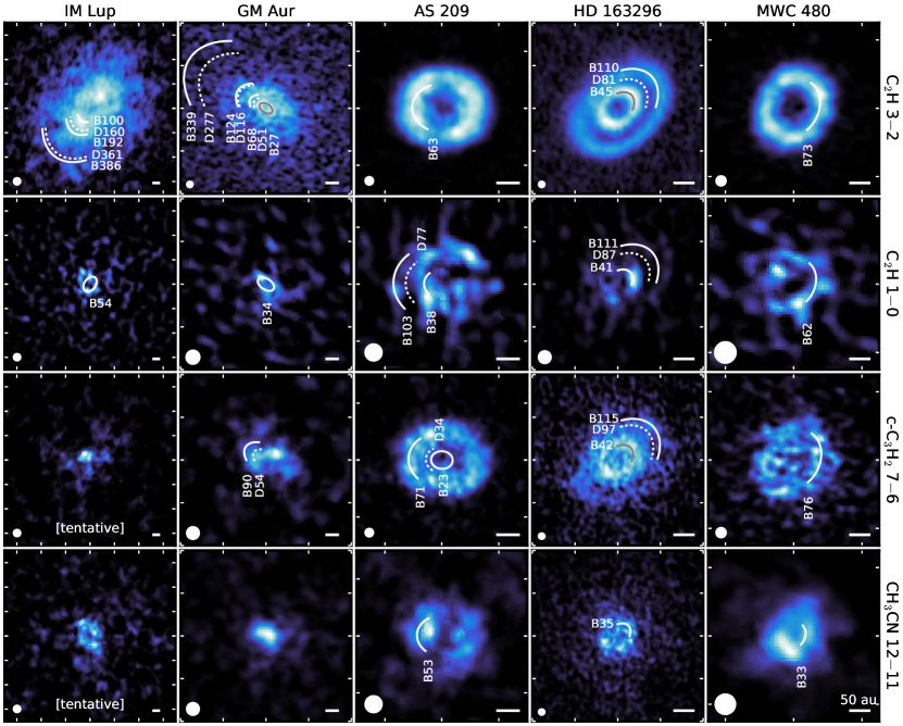
Figure 4: Zeroth moment maps of C₂H, c-C₃H₂, CH₃CN lines for the MAPS sample, ordered from left to right by increasing stellar mass (see Table 1 in Oberg et al. (2021)). Axes are angular offsets from the disk center with each white tick mark represents a spacing of 1^′′. Color stretches were individually optimized and applied to each panel to increase the visibility of substructures. Care should thus be taken when comparing between panels, and instead, we recommend using the corresponding radial profiles in Figure 10 for this purpose. Chemical substructures from Table 3 in the form of rings and gaps are marked by solid and dotted arcs, respectively, with azimuthal extents and colors chosen for maximal visual clarity. The synthesized beam and a scale bar indicating 50 au is shown in the lower left and right corner, respectively, of each panel.

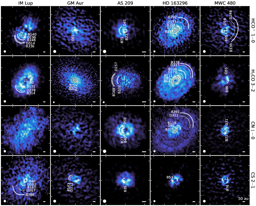
Figure 5: Zeroth moment maps of HCO⁺, H₂CO, CN, and CS lines for the MAPS sample, ordered from left to right by increasing stellar mass (see Table 1 in Oberg et al. (2021)). Axes are angular offsets from the disk center with each white tick mark represents a spacing of 2^′′. Color stretches were individually optimized and applied to each panel to increase the visibility of substructures. Care should thus be taken when comparing between panels, and instead, we recommend using the corresponding radial profiles in Figure 11 for this purpose. Chemical substructures from Table 3 in the form of rings and gaps are marked by solid and dotted arcs, respectively, with azimuthal extents and colors chosen for maximal visual clarity. The synthesized beam and a scale bar indicating 50 au is shown in the lower left and right corner, respectively, of each panel.

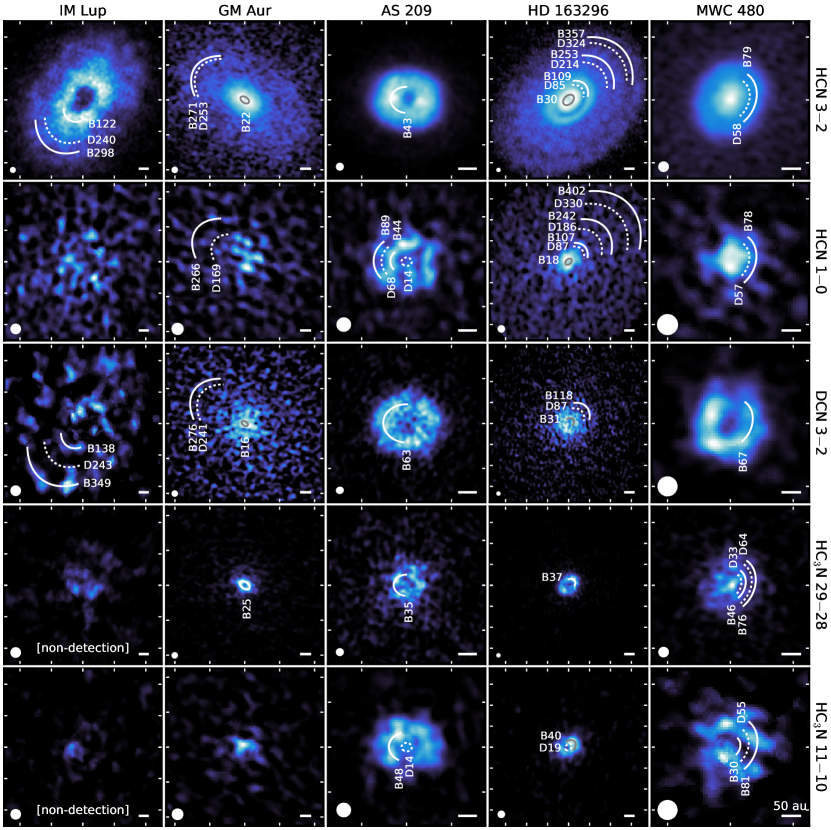
Figure 6: Zeroth moment maps of HCN, DCN, and HC₃N lines for the MAPS sample, ordered from left to right by increasing stellar mass (see Table 1 in Oberg et al. (2021)). Axes are angular offsets from the disk center with each white tick mark represents a spacing of 1^′′. Color stretches were individually optimized and applied to each panel to increase the visibility of substructures. Care should thus be taken when comparing between panels, and instead, we recommend using the corresponding radial profiles in Figure 12 for this purpose. Chemical substructures from Table 3 in the form of rings and gaps are marked by solid and dotted arcs, respectively, with azimuthal extents and colors chosen for maximal visual clarity. The synthesized beam and a scale bar indicating 50 au is shown in the lower left and right corner, respectively, of each panel.

In addition to zeroth moment maps, we also produced maps of the spectral line maximum intensity, or “peak intensity map,” and of the intensity-weighted average velocity, or “rotation map”. Peak intensity maps were generated using the “quadratic” method of bettermoments, which fits a quadratic curve to the channel with the peak intensity and two adjacent channels (Teague & Foreman-Mackey, 2018). This approach better recovers the true line peak when the line profile is only sparsely sampled, unlike traditional eighth moment maps, which are limited by the spectral resolution of the data. A full set of peak intensity maps are shown in Appendix C, which although not directly analyzed in this work, are provided for completeness. Rotation maps of the line center were also created using the “quadratic” method of bettermoments, which produces a less biased map for highly-flared disks than first moment maps. These maps are not shown here but see Teague et al. (2021) for a detailed presentation and discussion of CO rotation maps.

This set of maps – zeroth moment, rotation, peak intensity – are provided as VADPs and are available to the community through our dedicated website hosted by ALMA (https://almascience.nrao.edu/alma-data/lp/maps). Moment maps were generated for all lines covered in MAPS (see Tables 2 and 3, Oberg et al., 2021), not just those considered here, and for all available angular resolutions (see Table 5, Oberg et al., 2021). A corresponding set of maps, derived as described above, for the non-continuum-subtracted images are also provided. As all maps are generated from bettermoments, they also include a corresponding map of statistical uncertainty for each measured quantity, as described in Teague & Foreman-Mackey (2018). Scripts to generate the hybrid zeroth moment maps used for presentational purposes will also be made publicly available.

2.3 Radial intensity profiles

A radial line intensity profile provides a helpful one-dimensional representation of emission in protoplanetary disks as a function of radius. In this subsection, we describe the process by which we generate radial profiles, including details of the deprojection process and extraction methods, and how we select those profiles which best reveal observed chemical substructures.

We generated radial profiles using the radial_profile function in the Python package GoFish (Teague, 2019b) to deproject the zeroth moment maps. Radial bin sizes are calculated as 1/4 of the full-width at half-maximum (FWHM) of the synthesized beam, which corresponds to about 1.5-2 pixels. The uncertainty of the measured intensity in each radial bin is estimated as the standard error on the mean in the annulus or arc over which the emission was averaged. An advantage of this empirical error estimate is that it includes uncertainties related to the entire imaging and moment map generation process. However, uncertainties are artificially larger in regions with large intrinsic azimuthal variation. One such example is molecular emission from regions highly elevated above the disk midplane, which manifests as a large ‘X’ morphology in many of the panels showing CO and ¹³CO in Figure 3. This ‘X’ shape arises from spatially separated isovelocity contours in the inter-axis regions (e.g., see Figure 4, Keppler et al., 2019), which allows emission from both sides of the disk to reach the observer.

In addition to extracting radial intensity profiles from the zeroth moment maps, we tested the method used in Teague & Loomis (2020a). There, the authors first corrected for the velocity structure of the disk, before azimuthally averaging the spectra and then integrating the line profiles (e.g., Yen et al., 2016) in GoFish. There were negligible differences between these methods, and we opted to use the radial profiles of the zeroth moment maps for simplicity.

For each line, we generated an azimuthally-averaged profile and a set of profiles extracted along the major axis of each disk, where emission was averaged within varying azimuthal wedges, namely $\pm$15^∘, $\pm$30^∘, and $\pm$45^∘. We manually selected wedge sizes that maximized the relative contrasts of individual substructures, while still maintaining high fidelity. Narrower wedges taken along the disk major axis often resulted in features with sharper contrasts and were used whenever the SNR allowed. This is the result of a lower effective spatial resolution along the minor axis of an inclined disk, which if included, can smear radial features. However, if decreasing the wedge size did not lead to the emergence of any new features or the sharpening of existing substructures, we used progressively larger wedge sizes, up to a complete azimuthal average, to improve the SNR and overall smoothness of profiles. The selections for each radial profile are summarized in Table 1.

Figure 7 shows an example of this process. For medium-to-strong lines with well-defined substructures, such as the inner emission ring at ${\sim}$50 au in c-C₃H₂ 7–6 in HD 163296, narrow wedges result in higher contrast features and more accurate determinations of radial locations. Narrow wedges also often amplify substructures not evident when using wider azimuthal wedges. This is the case for the outer ring at ${\sim}$110 au in c-C₃H₂ 7–6, which is not present in the azimuthally averaged radial profile, but is clearly seen when using a $\pm$30^∘ wedge. For lines with smoother, more extended radial morphologies, like H₂CO 3–2 in HD 163296, an azimuthally averaged profile is sometimes most effective in identifying features, e.g., the dip at ${\sim}$170 au.

In cases where line emission is originating from a layer substantially higher than the disk midplane, we must take this emitting surface into account to accurately deproject the observations into annuli of constant radius. We deprojected radial profiles using the derived surfaces from Law et al. (2021), as indicated in Table 1, for those lines with meaningful constraints on their emission surfaces, namely CO 2–1, ¹³CO 2–1, HCN 3–2, and C₂H 3–2 (see Appendix D). Otherwise, for simplicity, we assumed that the line emission is arising from the midplane, i.e., $z/r=0.0$. Further testing confirmed that the radial intensity profiles of those lines lacking explicit emission surface determinations are consistent for any reasonable choice of assumed surfaces (e.g., $z/r=0.0,0.1,0.2$).

The AS 209 disk suffers from cloud absorption at $v_{\rm{LSR}}~{}\lesssim~{}5$ km s^-1 (Öberg et al., 2011b). This results in reduced CO 2–1 flux toward the west half of its disk (Huang et al., 2016; Guzmán et al., 2018b), which is also clearly seen in the MAPS data (Figure 3). In addition to CO 2–1, significant absorption is present in HCO⁺ 1–0, while more modest east-to-west flux asymmetries are noted in C₂H 1–0 and HCN 1$-$0. For these lines, we adopted an asymmetric $\pm 55^{\circ}$ wedge, as in Teague et al. (2018), that was applied to the uncontaminated eastern half. Otherwise, no obvious azimuthal asymmetries were identified and all other lines were assumed to be azimuthally symmetric, but see Le Gal et al. (2021) for a exploration of potential asymmetries in CS.

Figures 9, 10, 11, and 12 show the set of radial intensity profiles selected here to highlight radial chemical substructures. These radial profiles, along with those generated from all combinations of wedge sizes, are provided as publicly-available VADPs. Radial profiles for all lines covered in MAPS, including those not analyzed here (see Tables 2 and 3, Oberg et al., 2021), and for all imaged angular resolutions (see Table 5, Oberg et al., 2021), are also available. Additionally, as for the moment maps, a corresponding set of radial profiles for the non-continuum-subtracted images are included. See Section 7 for more details and a full listing of available VADPs.

Table 1: Summary of Radial Profiles

	IM Lup		GM Aur		AS 209		HD 163296		MWC 480
Linea	Type	Surface	Type	Surface	Type	Surface	Type	Surface	Type	Surface
CO 2$-$1	30∘/$0\farcs 15$	Y	15∘/$0\farcs 15$	Y	55${}^{\circ,\,d}$/$0\farcs 15$	Y	15∘/$0\farcs 15$	Y	15∘/$0\farcs 15$	Y
13CO 2$-$1	360∘/$0\farcs 15$	Y	30∘/$0\farcs 15$	Y	30∘/$0\farcs 15$	N	15∘/$0\farcs 15$	Y	360∘/$0\farcs 15$	N
13CO 1$-$0	360∘/$0\farcs 30$	N	45∘/$0\farcs 30$	N	30∘/$0\farcs 30$	N	30∘/$0\farcs 30$	N	45∘/$0\farcs 30$	N
C18O 2$-$1	45∘/$0\farcs 15$	N	30∘/$0\farcs 15$	N	30∘/$0\farcs 15$	N	45∘/$0\farcs 15$	N	360∘/$0\farcs 15$	N
C18O 1$-$0	45∘/$0\farcs 30$	N	45∘/$0\farcs 30$	N	45∘/$0\farcs 30$	N	30∘/$0\farcs 30$	N	360∘/$0\farcs 30$	N
C2H 3$-$2	45∘/$0\farcs 30$	N	45∘/$0\farcs 15$	N	30∘/$0\farcs 15$	N	15∘/$0\farcs 15$	Y e	30∘/$0\farcs 15$	N
C2H 1$-$0	360∘/$0\farcs 30$	N	360∘/$0\farcs 30$	N	55${}^{\circ,\,d}$/$0\farcs 30$	N	30∘/$0\farcs 30$	N	360∘/$0\farcs 30$	N
c-C3H2 7$-$6	360∘/$0\farcs 30$	N	30∘/$0\farcs 30$	N	360∘/$0\farcs 15$	N	30∘/$0\farcs 15$	N	30∘/$0\farcs 30$	N
H2CO 3$-$2	45∘/$0\farcs 30$	N	30∘/$0\farcs 15$	N	30∘/$0\farcs 15$	N	360∘/$0\farcs 30$	N	30∘/$0\farcs 30$	N
HCO+ 1$-$0	30∘/$0\farcs 30$	N	30∘/$0\farcs 30$	N	55${}^{\circ,\,d}$/$0\farcs 30$	N	360∘/$0\farcs 30$	N	30∘/$0\farcs 30$	N
CS 2$-$1	30∘/$0\farcs 30$	N	360∘/$0\farcs 30$	N	45∘/$0\farcs 30$	N	360∘/$0\farcs 30$	N	360∘/$0\farcs 30$	N
CN 1$-$0 b	360∘/$0\farcs 30$	N	360∘/$0\farcs 30$	N	30∘/$0\farcs 30$	N	30∘/$0\farcs 30$	N	30∘/$0\farcs 30$	N
HCN 3$-$2	360∘/$0\farcs 15$	N	30∘/$0\farcs 15$	N	30∘/$0\farcs 15$	N	30∘/$0\farcs 15$	Y e	30∘/$0\farcs 15$	N
HCN 1$-$0	360∘/$0\farcs 30$	N	45∘/$0\farcs 30$	N	55${}^{\circ,\,d}$/$0\farcs 30$	N	30∘/$0\farcs 30$	N	30∘/$0\farcs 30$	N
DCN 3$-$2	360∘/$0\farcs 30$	N	360∘/$0\farcs 15$	N	360∘/$0\farcs 15$	N	30∘/$0\farcs 30$	N	360∘/$0\farcs 30$	N
HC3N 29$-$28	360∘/$0\farcs 30$	N	360∘/$0\farcs 15$	N	360∘/$0\farcs 15$	N	30∘/$0\farcs 15$	N	360∘/$0\farcs 15$	N
HC3N 11$-$10	360∘/$0\farcs 30$	N	360∘/$0\farcs 30$	N	45∘/$0\farcs 30$	N	30∘/$0\farcs 30$	N	45∘/$0\farcs 30$	N
CH3CN 12$-$11 c	360∘/$0\farcs 30$	N	360∘/$0\farcs 30$	N	360∘/$0\farcs 30$	N	30∘/$0\farcs 15$	N	360∘/$0\farcs 30$	N

Note. — Type indicates the wedge size of the radial profile used in this analysis and FWHM of the synthesized beam of the image. Profiles were extracted along the disk major axis in an azimuthal wedge twice (i.e., $\pm$) that of the listed value, except for those listed as 360^∘, which denote an azimuthally-averaged profile. Surface choices (Y/N) are taken from Law et al. (2021).

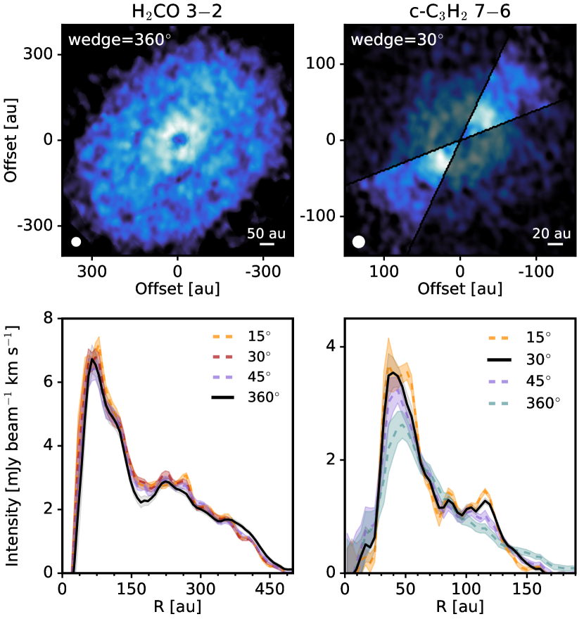
Figure 7: Effects of wedge sizes on radial intensity profiles. The top row shows zeroth moment maps of H₂CO 3–2 (left column) and c-C₃H₂ 7–6 (right column) in HD 163296. The synthesized beam and a scale bar indicating either 20 or 50 au is shown in the lower left and right corner, respectively, of each panel. Axes are labeled as offsets in au from the disk center. The bottom row shows the radial intensity profiles. Radial profiles, as indicated by the legend color, are either azimuthally-averaged or extracted from a wedge size of $\pm$15^∘, $\pm$30^∘, $\pm$45^∘ along the disk major axis. The selected profile, as in Table 1, is indicated as a solid black line. Shaded regions show the 1$\sigma$ scatter at each radial bin (i.e., arc or annulus) divided by the ratio of the square root of bin circumference and FWHM of the synthesized beam.

3 Characterization of Disk Features

3.1 Radial locations of substructures

We adopt a chemical substructure nomenclature analogous to that established for annular dust substructure (Huang et al., 2018b, 2020). Each substructure is labeled with its radial location rounded to the nearest whole number in astronomical units and is preceded by either “B” (for “bright”) or “D” (for “dark”) depending on if the emission represents a local maximum or minimum, respectively. These features are also frequently referred to as “rings” or “gaps,” respectively (e.g., Öberg et al., 2015a; Bergin et al., 2016). In a few cases, e.g., single isolated rings, the term substructure is a misnomer but is a useful convention for the purposes of a homogeneous comparison. Below, we describe the procedure used to identify, characterize, and label these substructures.

For each intensity profile exhibiting radial substructure, we model the profile as a sum of one or more Gaussian profiles using the Levenberg-Marquardt minimization implementation in LMFIT (Newville et al., 2020). Before fitting, the number of component Gaussian profiles was fixed via visual inspection. The fitted centers of each Gaussian are taken to be the radial location of each feature and are reported in Table 3. The majority of lines are well-suited to this approach due to the high contrasts and well-separated nature of their substructural features. Even in cases when components overlap, Gaussian decomposition captures the underlying features. On occasion, it was necessary to manually restrict the fitting range to better reproduce the observed profiles. This was most often necessary in cases where plateau-like emission was located on one side of an emission ring, resulting in incorrectly skewed fits. In cases such as this, accurate determinations of the radial location of line peaks or gaps were prioritized and attempts were not made to fully reproduce highly skewed or asymmetric features. Substructures displaying notable deviations from Gaussian shapes are discussed in more detail in Section 3.3.

Unlike the majority of other species, the CO lines are not composed of well-separated, distinct features, but instead of numerous low-contrast features on top of a broad power-law-like background. As a result, it was often necessary to first fit and remove this broad component to accurately characterize the substructural features. This was done by fitting either an exponential power-law component or one or more broad Gaussians. Figure 8 shows an example of this Gaussian decomposition process.

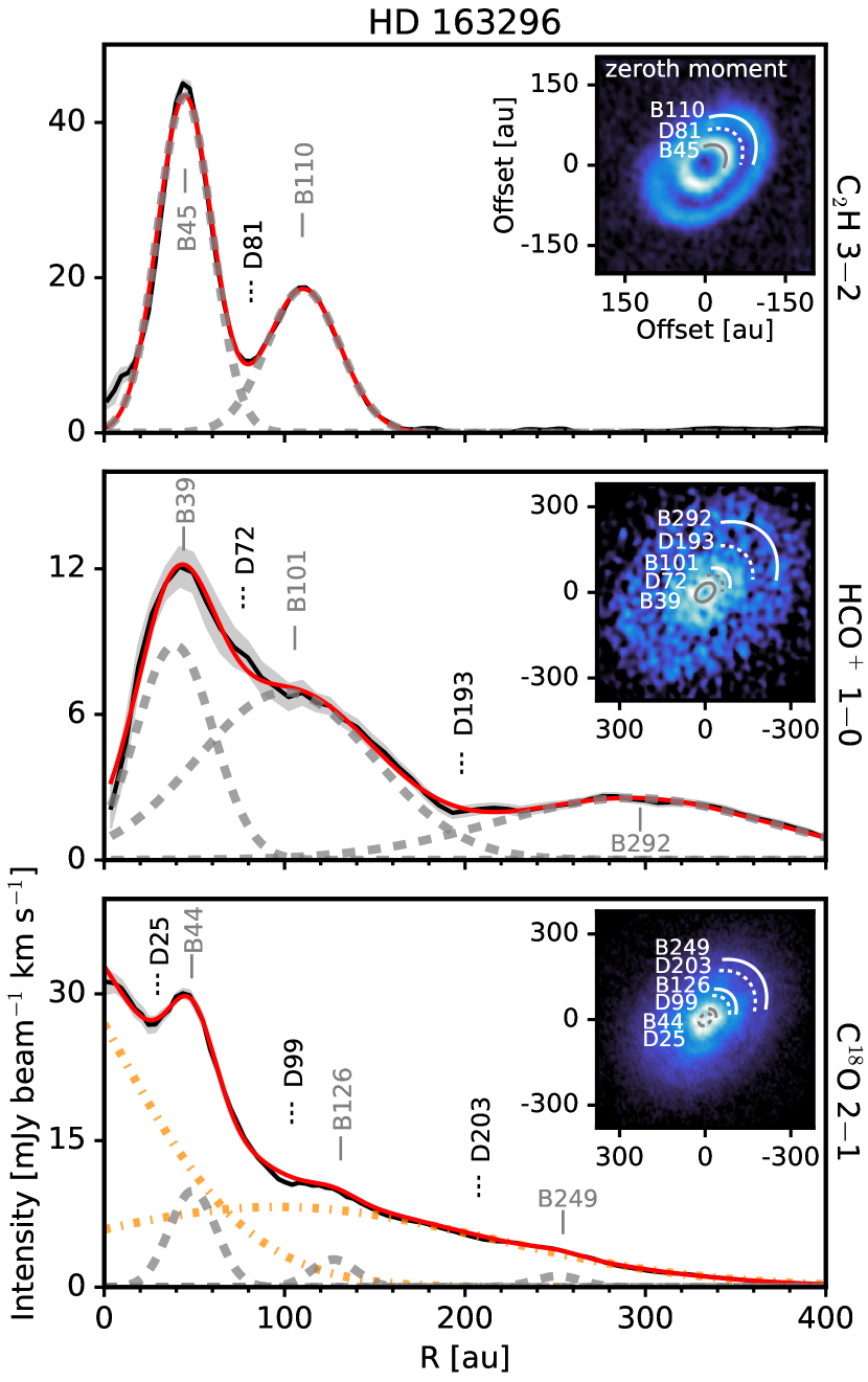
Figure 8: Example Gaussian decomposition for C₂H 3–2 (top), HCO⁺ 1–0 (middle), and C¹⁸O 2–1 (bottom) in HD 163296. The red solid line indicates the composite fit, while individual Gaussian profiles are shown as dashed gray lines. The orange dash-dotted lines in the bottom panel are Gaussians used to remove the broad and smoothly decreasing background in C¹⁸O 2–1. The intensities of the low-amplitude Gaussians at ${\sim}$130 and 250 au have each been multiplied by a factor of 3 for visual clarity. The insets show zeroth moment maps with axes labeled as offsets in au from the disk center. Chemical substructures are marked by solid and dotted arcs, indicating bright and dark features, respectively.

While Gaussian profiles provide a natural characterization of emission rings, they do not as readily describe the radial locations of gaps. Only in some cases, i.e., CO lines, where we could fit and remove the underlying smooth profile, was it possible to directly fit gaps with (inverted) Gaussian profiles. However, for the majority of gaps, we instead report the local minimum of each emission gap as its radial location. The positional uncertainty of each minima is estimated as the width of one radial bin (from 4 au to 13 au, depending on transition frequency and source distance).

For certain lines, e.g., HCO⁺ 1–0, H₂CO 3–2 and CN 1–0, as shown in Figure 11, there are regions of the radial profiles which represent bona fide annular substructures, i.e., deviations from a smooth profile, but are not in the form of distinct emission rings or gaps. Such features are often referred to as either emission “plateau” or “shoulders” (e.g., Huang et al., 2018a, b, 2020). For consistency, we define those deviations that have relatively narrow radial extents as shoulders, e.g., B192, C₂H 3$-$2 in IM Lup (Figure 10); B46 and B76 in HC₃N 29–28 in MWC 480 (Figure 12), while those that display nearly constant excess emission out to large radii as plateau, e.g., HCN 1–0 in IM Lup (Figure 12); HCO⁺ 1–0 in GM Aur (Figure 11). Emission plateaus, which lack a single well-defined radial position, are not explicitly listed in Table 3, but a few prominent examples are instead noted in Table 4. In contrast, emission shoulders are more well-defined and, when possible, were characterized using Gaussian profiles; otherwise, their radial positions were catalogued visually.

Following Huang et al. (2018b), the inner and outer edges of an emission shoulder were denoted with the prefixes “D” and “B,” respectively, followed by the radial location in au rounded to the nearest integer. Even in cases when the outer edge of a “B” substructure was well-fit with a Gaussian profile, the inner edge still needed to be visually identified. As this method is more subjective than either Gaussian fitting or local extrema identification, approximate locations are listed in Table 3 without formal error estimates. However, the uncertainties should be less than a synthesized beam.

Measurements that are derived from Gaussian fittings are indicated as “G” in Table 3, while those based on the identification of local extrema in the radial profiles are labeled “R”. Visual identifications are denoted as “V.” Figures 9, 10, 11, and 12 show the labeled radial intensity profiles. Figure 30 in Appendix E provides logarithmically-scaled radial intensity profiles for all CO lines to more clearly show low-contrast substructures, especially those at large radii.

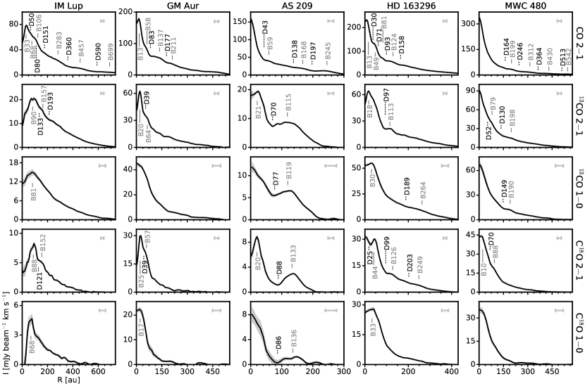
Figure 9: Deprojected radial intensity profiles of CO lines, as indicated in Table 1, for the MAPS sample, ordered from left to right by increasing stellar mass. Gray shaded regions show the 1$\sigma$ scatter at each radial bin (i.e., arc or annulus) divided by the ratio of the square root of bin circumference and FWHM of the synthesized beam. Solid gray lines mark emission rings and dotted black lines mark gaps, as listed in Table 3. The FWHM of the synthesized beam is shown by a horizontal bar in the upper right corner of each panel.

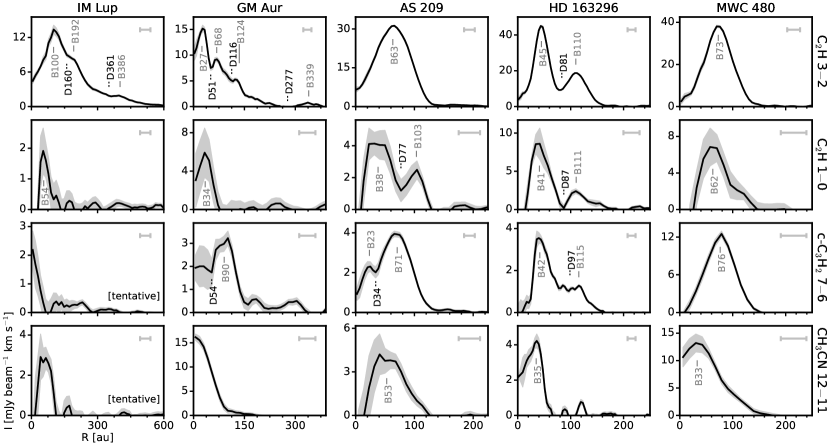
Figure 10: Deprojected radial intensity profiles of C₂H, c-C₃H₂, and CH₃CN lines, as indicated in Table 1. An apparent emission ring at 60 au is present in CH₃CN 12–11 in IM Lup, but as this line is only tentatively detected (Ilee et al., 2021), we do not label this substructure and omit it from further analysis. Otherwise, as in Figure 9.

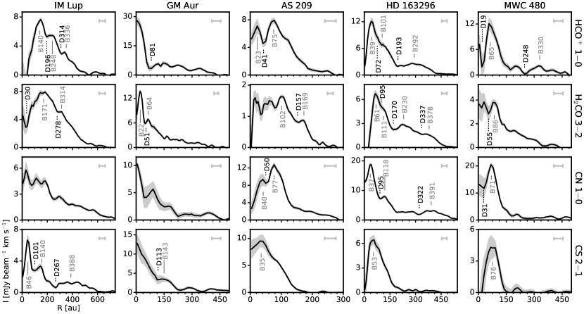
Figure 11: Deprojected radial intensity profiles of HCO⁺, H₂CO, CN, and CS lines, as indicated in Table 1. Otherwise, as in Figure 9.

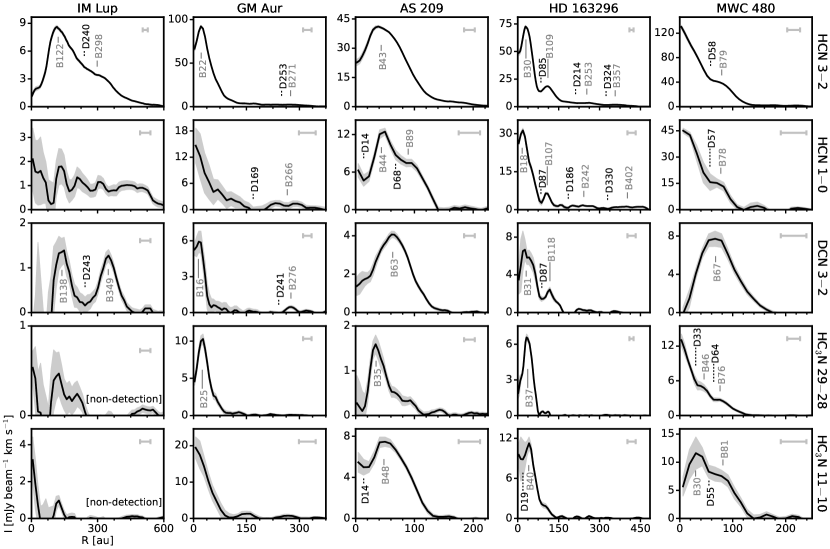
Figure 12: Deprojected radial intensity profiles of HCN, DCN, and HC₃N lines, as indicated in Table 1. Otherwise, as in Figure 9.

3.2 Widths and depths of substructures

Defining the widths and depths of substructures is less straightforward than identifying their radial locations. For emission rings, which were modeled as Gaussian profiles, the FWHMs were taken to be the ring widths. For all gaps, we instead followed the empirical procedure outlined in Huang et al. (2018b). In brief, substructure widths were defined by the radial locations where the intensity is equal to the mean intensity of a consecutive ring-gap pair. For rings with emission profiles that can be modeled as isolated Gaussians, this definition reduces to approximately the FWHM, and as such, makes it a comparable metric for gap widths. A detailed description of this procedure, including treatment of various special cases, is found in Huang et al. (2018b).

The relative contrast of an adjacent gap-ring pair is defined by their intensity ratio. Specifically, gap depth is given as $I_{d}/I_{b}$, where the gap intensity $I_{d}$ is the intensity value at the radial position of the gap and $I_{b}$ is the intensity value at the radial position of the ring directly outside the gap. In a few cases, there was no suitable ring outside of the gap (D14 in HCN 1–0, HC₃N 11–10; D34 in c-C₃H₂ 7–6; and D50 in CN 1–0 for AS 209) and we used the ring interior for calculating the depth. Substructure widths and depths are listed in Table 3. We subsequently refer to gap depths according to their decrease in fractional intensity with deeper gaps having lower intensity ratios, e.g., an intensity ratio of $I_{d}/I_{b}$=0.2 indicates a gap depth of 80%.

Beam effects are not explicitly accounted for in these definitions and likely result in underestimating gap widths and overestimating ring widths compared to their true values. Similarly, gap depths may also be underestimated, as beam convolution reduces peak intensities and fills in gaps. While for clearly resolved features, the effects of beam smearing should be small, it becomes significant for features which have widths comparable to the beam size. Nonetheless, the adopted conventions are still useful for comparing substructures across the MAPS sample.

3.3 Additional and tentative substructures

To ensure that we did not miss the presence of extended but low SNR features in the radial profiles listed in Table 1, we inspected all tapered (0$\farcs$30) profiles and zeroth moment maps. The process revealed two additional C₂H 3$-$2 emission rings (B244, B368) in HD 163296, as shown in Figure 13. This outermost ring was previously detected by Bergner et al. (2019), while the narrower ring at 244 au is newly detected in the MAPS observations. As indicated in Table 3, we used the 0$\farcs$30 tapered resolution radial profile to fit both of these rings, as they are too low SNR in the 0$\farcs$15 resolution image for a robust characterization.

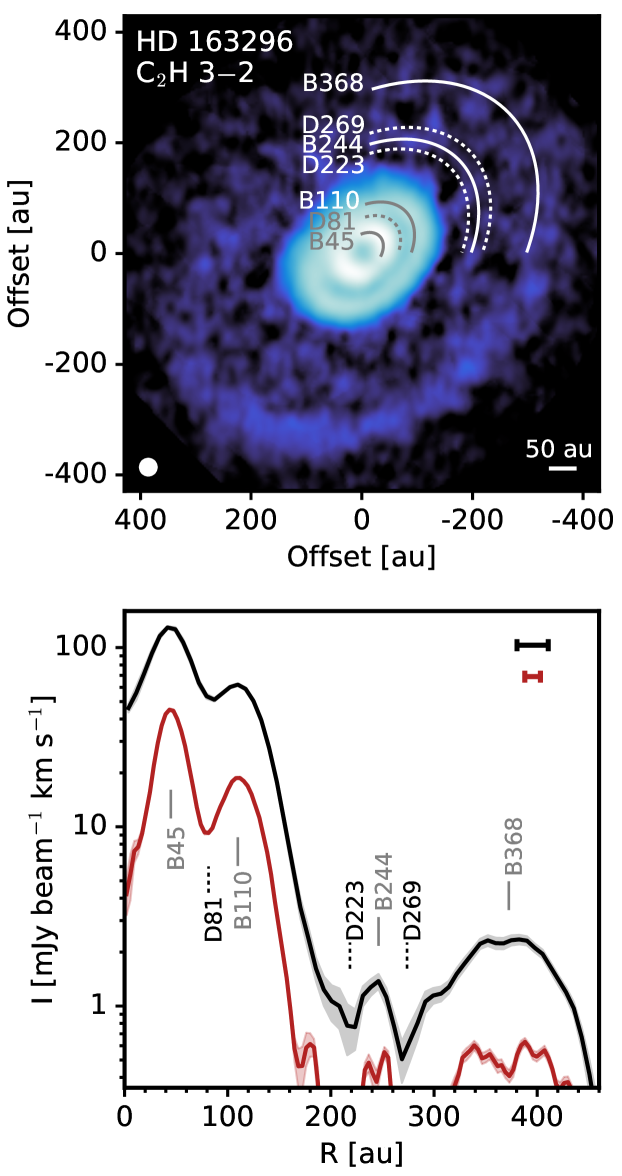
Figure 13: Zeroth moment map (top) and radial intensity profile (bottom) of C₂H 3$-$2 in HD 163296. An arcsinh color stretch has been applied to the zeroth moment map. The red and black curves show the 0$\farcs$15 and 0$\farcs$30 resolution profiles, respectively.

A few lines exhibit suggestive emission shoulders, which were not distinctive enough to be considered as independent substructural features, but may still indicate the presence of additional, marginally resolved emission rings. A full listing of such emission shoulders is provided in Table 4. We also catalogued lines that exhibit prominent emission plateaus, e.g., H₂CO 3–2, HCO⁺ 1–0 in GM Aur (Figure 11); HCN 1–0 in IM Lup (Figure 12). All MAPS disks exhibit diffuse, radially-extended CN 1–0 emission, which is discussed further in Bergner et al. (2021).

The radial intensity profiles of a few emission rings deviate from Gaussian or otherwise symmetric profiles. Asymmetric profiles such as these may be the result of two unresolved rings or reflect true ring asymmetries. While we did not attempt a detailed characterization of such asymmetries, some notable instances are listed in Table 4. In particular, HCN 3$-$2, HC₃N 11–10 in AS 209 (Figure 12) both display asymmetric tails toward larger radii in their emission rings. More modest asymmetries are seen in several other lines, such as CS 2–1 in HD 163296 and DCN 3–2 in MWC 480.

3.4 Annular continuum substructures

All disks have existing high angular resolution observations of their millimeter continua (Long et al., 2018a; Huang et al., 2018b) and sometimes in several ALMA bands (e.g., Huang et al., 2020). However, due to the sensitivity of the MAPS observations, we detected new substructures in the outer continuum disks of IM Lup (D209, B220) and MWC 480 (D149, B165). In IM Lup, this outer ring had been tentatively seen in the lower resolution (0$\farcs$3) observations of Cleeves (2016). In MWC 480, this additional dust ring, although not seen in previous imaging, had been inferred from visibility model fitting (Long et al., 2018a; Liu et al., 2019).

The characteristics of these new continuum substructures are reported in Table 5. We generated continuum radial profiles and identified annular features, as in Sections 2.3 and 3.1–3.2, respectively. All annular substructures were characterized using azimuthally-averaged profiles to increase SNR in the outer radii and with the 260 GHz continuum, which possesses the highest angular resolution (${\sim}$0$\farcs$1). For all disks, the other three continuum frequency settings were inspected, but none revealed any additional substructures not present in the 260 GHz continuum, as illustrated in Figure 14.

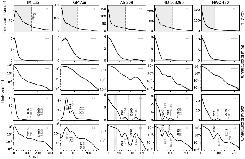
Figure 14: Deprojected radial intensity profiles of the 90 GHz and 260 GHz continua compared to CO 2–1, ordered from left to right by increasing stellar mass. The outer edge of the millimeter continuum (R_edge) is shown as a gray shaded region in the CO 2–1 profiles. Both linear scale and log scale continuum radial intensity profiles are shown. Gray shaded regions show the 1$\sigma$ scatter at each radial bin (i.e., arc or annulus) divided by the ratio of the square root of bin circumference and FWHM of the synthesized beam. Solid gray lines mark emission rings and dotted black lines mark gaps, as listed in Table 5. Vertical solid and dotted lines indicate millimeter continuum rings and gaps, respectively, that are unresolved in our observations. The FWHM (i.e., 0$\farcs$15 for CO 2–1 and minor axis for continuum images) of the synthesized beam is shown by a horizontal bar in the upper right corner of each panel.

Although GM Aur has extensive continuum observations (Huang et al., 2020), the individual annular substructures lack reported widths and depths. As a result, we refit all substructures self-consistently and found that all radial locations were within 2–5 au of those reported in Huang et al. (2020). Similarly, previous millimeter continuum observations exist for MWC 480 (Long et al., 2018a; Liu et al., 2019), but the MAPS observations have a higher spatial resolution and improved RMS, as detailed in Sierra et al. (2021). We refit the MWC 480 continuum substructures and found differences in derived radial locations of no more than 3 au.

To self-consistently compare continuum and chemical substructures, we refit those continuum substructures which have been previously catalogued in DSHARP at higher spatial resolutions. All refitted values, and their corresponding DSHARP names, are marked in Table 5. In Table 5, we also list those substructures identified by Huang et al. (2018b, 2020) at small radii or with very narrow widths that we did not detect due to our lower spatial resolution. Overall, we find close agreement between the radial positions reported in DSHARP and those derived from our refitting process with a maximum difference of any individual substructure of no more than 4 au. This consistency indicates that the derived substructure characteristics do not depend strongly on the details of the fitting process. We also emphasize that refitted values are solely for the purposes of self-consistent comparison and that those previously derived from higher angular resolution observations ultimately represent more accurate radial locations and widths. An overview of continuum radial intensity profiles for the MAPS sources with labeled continuum substructures is shown in Figure 14. For a more detailed analysis of the continuum, see Sierra et al. (2021).

3.5 Gas disk radii

Note: The calculation of gas disk sizes in the published article initially omitted the necessary factor of $2\pi r$ when computing the cumulative sums, i.e., the integral of a radial function has an areal element of $2\pi rdr$. Please see the associated Erratum for a full update of this Section; while the text is unchanged, we have corrected the values shown in Table 2 and Figures 15-16.

To explore the relative size of line emission in the MAPS disks, we computed the radius of the gas disk for each line. We used a method similar to that of Ansdell et al. (2018). We first measured a total line flux, taken as the asymptotic value of the azimuthally-averaged radial intensity profiles. We then define R_gas as the radius which encloses 90% of this total flux. The measured values are listed in Table 2 and shown in Figure 15. The estimated uncertainty includes the uncertainty in radial location equal to one bin, as for the radial features, and the uncertainty in the line fluxes.

Table 2: Gas Disk Sizes

Line	Disk Size (au)
	IM Lup	GM Aur	AS 209	HD 163296	MWC 480
CO 2$-$1	753 $\pm$ 6	616 $\pm$ 9	272 $\pm$ 4	459 $\pm$ 4	573 $\pm$ 7
13CO 2$-$1	540 $\pm$ 7	427 $\pm$ 9	196 $\pm$ 5	364 $\pm$ 4	419 $\pm$ 7
13CO 1$-$0	543 $\pm$ 16	410 $\pm$ 16	190 $\pm$ 10	340 $\pm$ 8	392 $\pm$ 17
C18O 2$-$1	404 $\pm$ 14	297 $\pm$ 24	176 $\pm$ 5	301 $\pm$ 4	326 $\pm$ 11
C18O 1$-$0	436 $\pm$ 45	219 $\pm$ 26	160 $\pm$ 9	275 $\pm$ 11	312 $\pm$ 40
C2H 3$-$2	478 $\pm$ 18	200 $\pm$ 12	115 $\pm$ 5	352 $\pm$ 8	120 $\pm$ 7
C2H 1$-$0	114 $\pm$ 15	56 $\pm$ 17	110 $\pm$ 9	153 $\pm$ 55	113 $\pm$ 14
c-C3H2 7$-$6	$\ldots$	169 $\pm$ 16	112 $\pm$ 8	162 $\pm$ 20	122 $\pm$ 13
H2CO 3$-$2	474 $\pm$ 15	366 $\pm$ 13	202 $\pm$ 7	404 $\pm$ 9	375 $\pm$ 29
HCO+ 1$-$0	492 $\pm$ 50	389 $\pm$ 25	199 $\pm$ 15	385 $\pm$ 13	408 $\pm$ 26
CS 2$-$1	592 $\pm$ 21	197 $\pm$ 13	124 $\pm$ 10	177 $\pm$ 11	114 $\pm$ 31
HCN 3$-$2	418 $\pm$ 9	295 $\pm$ 13	159 $\pm$ 5	361 $\pm$ 4	176 $\pm$ 24
HCN 1$-$0	638 $\pm$ 45	306 $\pm$ 100	115 $\pm$ 9	447 $\pm$ 9	92 $\pm$ 47
DCN 3$-$2	397 $\pm$ 17	76 $\pm$ 10	112 $\pm$ 6	161 $\pm$ 37	126 $\pm$ 12
HC3N 29$-$28	$\ldots$	77 $\pm$ 11	93 $\pm$ 5	86 $\pm$ 6	98 $\pm$ 8
HC3N 11$-$10	$\ldots$	71 $\pm$ 26	108 $\pm$ 10	126 $\pm$ 16	126 $\pm$ 15
CN 1$-$0	594 $\pm$ 18	412 $\pm$ 16	231 $\pm$ 9	482 $\pm$ 9	530 $\pm$ 16
CH3CN 12$-$11	90 $\pm$ 12	100 $\pm$ 21	98 $\pm$ 10	54 $\pm$ 5	114 $\pm$ 14
90 GHz continuum	222 $\pm$ 10	171 $\pm$ 14	123 $\pm$ 8	111 $\pm$ 6	105 $\pm$ 13
260 GHz continuum	242 $\pm$ 4	194 $\pm$ 5	128 $\pm$ 3	139 $\pm$ 3	111 $\pm$ 5

Note. — Disk size was computed as the radius which encloses 90% of the total disk flux (see Section 3.5). Note that this is often smaller than the total radial extent of an emission line due to the presence of diffuse, low flux emission at large radii.

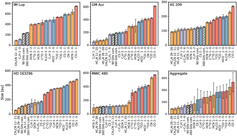
Figure 15: Gas disk size for all lines organized by increasing sizes within each disk. Sizes are color-coded by species, as described in Section 3.5. The size of the 90 GHz and 260 GHz continuum disks are shown as gray, hatched bars for comparison. The aggregate panel shows mean sizes of each line across the MAPS disks with error bars showing the standard deviation. Disk sizes are defined as the radius containing 90% of total flux.

Gas disk sizes span a wide range for individual transitions within a disk and across the MAPS sample. IM Lup has the largest disk with the most extended lines having R${}_{\rm{gas}}\gtrsim 450$ au, while the AS 209 disk is the most compact, having a maximum R_gas of only ${\sim}$200 au. In general, the CO lines and CN 1–0, HCO⁺ 1–0, and H₂CO 3–2 are the largest, while the nitriles are the smallest, with HC₃N 29–28 and CH₃CN 12–11 typically presenting the most compact radii in all disks. The hydrocarbons C₂H and c-C₃H₂ are also found in the bottom quartile of sizes. No clear trends are found when comparing Band 3 and Band 6 transitions from the same molecule, and in general, R_gas values are not systematically larger in Band 3 or Band 6, as would have been expected if we were resolution or sensitivity limited, respectively. Only in a few instances of especially weak lines, i.e., C₂H 1–0 in IM Lup and GM Aur, did we find substantially smaller sizes in Band 3 versus the Band 6 line of the same molecule, which for these particular cases, may suggest artificially smaller Band 3 lines due to insufficient sensitivity.

Lines are color-coded in Figure 15, and in subsequent analysis, according to the following groupings: CO isotopologues (red), nitriles (orange), hydrocarbons C₂H, c-C₃H₂ (purple), and CS, H₂CO, HCO⁺ (blue). The first three groupings are, in part, motivated by chemical similarity, as each nitrile has a $-$C$\equiv$N functional group and hydrocarbons are exclusively made up of hydrogen and carbon atoms. These categories are also in qualitative agreement with radial emission morphologies visually identified when comparing radial profiles. The grouping of CS, H₂CO, and HCO⁺ is, however, one of convenience, as these molecules are not chemically similar to other species in our sample, nor with one another.

Figure 15 suggests that O-poor organic chemistry (e.g., the hydrocarbons C₂H, c-C₃H₂ and nitriles HC₃N, CH₃CN) is, on average, quite compact, while CO and its inorganic and organic derivatives are extended. This should result in a large scaled C/O gradient across the disk and implies that the inner 100 au of the disk, which is most relevant for planet formation, is more C-rich than perhaps disk-averaged line emission would suggest (for further discussion, see Alarcón et al., 2021; Bosman et al., 2021a). In further support of this interpretation, the formation of complex nitriles, such as HC₃N and CH₃CN, has been shown to be efficient at elevated C/O ratios (Le Gal et al., 2019a). This effect is most pronounced in AS 209, MWC 480, and to a lesser degree, GM Aur, which have nearly bimodal size distributions between the extended CO and related species versus the compact complex nitriles. In fact, for all MAPS disks, the complex nitriles are no larger than ${\sim}$120 au in size — and are often comparable to that of the continuum extent — despite the wide variations in CO disk sizes. This suggests an association with the millimeter continuum, where these molecules may be more easily destroyed at radii beyond the pebble disk due to, e.g., less shielding from radiation or increased gas-phase O-chemistry.

To explore the relationship between the continuum and gas disk sizes, we included the size of the 90 GHz and 260 GHz continuum, measured as for the molecular lines, in Figure 15. The 260 GHz continuum disk is typically ${\sim}$20–35% larger than that of the 90 GHz. The two exceptions to this trend are MWC 480, where they are nearly equal, and IM Lup, where the continuum disk at 260 GHz is 55% larger than at 90 GHz. The continua are smaller than nearly every line in the MAPS disks, except for GM Aur, where they are larger than about one-third of the lines considered here. We also calculated molecular line-to-dust size ratios, which spanned a wide range of 0.4 to 6 across individual lines in the MAPS disks. The ratios associated with the complex nitriles are typically ${<}$1.5, reflecting their compact spatial distributions that do not extend much beyond the continuum disk. In contrast, the CO lines are much more extended with ratios between 2–6. In general, we find large disk-to-disk variations in line size (${>}$100 au) with the exception of the complex nitriles and c-C₃H₂, which have size variations of only ${\sim}$40 au among the MAPS disks.

To assess how similar or different disks are in their gas sizes, we compared the rank ordering of lines within each disk against one another. To do so, we computed Spearman correlation coefficients for each pair of disks, as shown in Figure 16. All pairs of disks are positively correlated, indicating that while the substructure patterns vary dramatically across disks, the relative radial size distribution of lines is similar between the different sources. In fact, this similarity is nearly at a one-to-one ratio among the GM Aur, HD 163296, and MWC 480 disks.

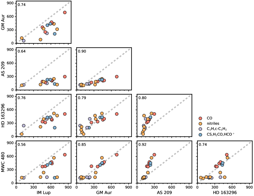
Figure 16: Gas disk size of chemical species in au for each disk plotted against one another. Spearman correlation coefficients are displayed in the upper left corners of each scatter plot. A one-to-one size ratio is shown as a gray dashed line. Sizes are color-coded by species according to the legend. In general, the distribution of sizes in different species is quite consistent among disks.

4 Properties of radial substructures

4.1 Distribution of radial substructure locations

Figures 3–6 and 9–12 show that substructures are observed at almost all radii where line emission is detected from ${\lesssim}$10 au to over 500 au, although the majority occur within 200 au. There is a wide range in the number of features seen across the different sources. The HD 163296 disk possesses the most chemical substructures with multiple emission rings and gaps in numerous lines, while IM Lup and GM Aur have smoother radial intensity profiles with relatively fewer well-defined substructures. AS 209 and MWC 480 show a single bright ring in the majority of lines and the occasional presence of emission shoulders and lower contrast substructures. Variations in the number of features observed within a single disk across different lines are also common, with HD 163296 demonstrating the most variability. For instance in HD 163296, HCN 3–2 has a set of four well-defined emission rings, but HC₃N 29–28 only has a single isolated ring. In contrast, AS 209 is the most consistent in its relative number of substructures across lines.

Figure 17 shows histograms of the positions of radial substructures in the MAPS sample. The number of rings and gaps in each disk generally decreases, although not monotonically, as a function of radius. As before, substructures are color-coded according to species. Each type of species displays radial substructure and when compared in aggregate, the relative number of rings contributed by each group is approximately constant in radius. In particular, in the inner 150 au, rings arising from each group occur in equal proportion, while the distribution of gaps has a modest deficit in substructures from hydrocarbons.

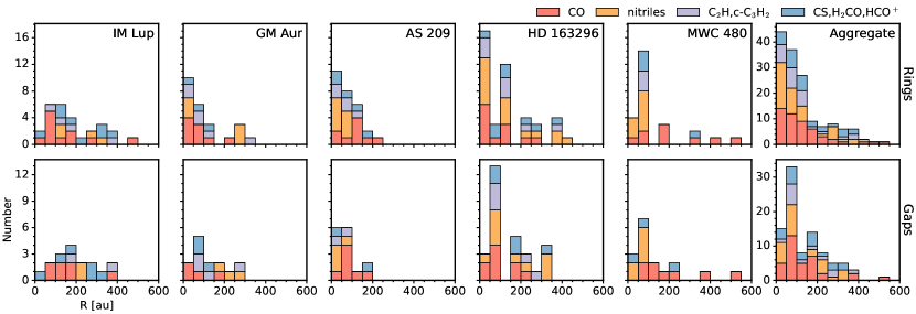
Figure 17: Histogram of radial locations of emission rings (top row) and gaps (bottom row) for each disk and in aggregate (columns). Substructures are color-coded by species according to the legend.

4.2 Distribution of substructure widths and depths

The measured widths and depths of substructures span a relatively wide range. Substructures have widths from ${<}10$ au to over 200 au, but the majority of features are less than 100 au wide. The deepest gaps have depths as low as 90%, but most gaps are considerably shallower with depths of ${\sim}$10–30%. The majority of extremely low contrast gaps, those on the order of a few percent, have widths that are comparable or smaller than the synthesized beam. Thus, their apparent shallowness may be a consequence of limitations in angular resolution. No trends with radius or species are identified in the gap depths of any MAPS source. Instead, there is significant variation in substructure depth at all radii and also among similar species.

Figure 18 shows substructure widths relative to their radial locations. Most features are spatially-resolved with measured widths that are larger than the FWHM of the beam, as shown by the gray dashed lines in Figure 18. However, the smallest measured widths are almost entirely located within the inner 100 au and should be treated as upper limits since they are often not clearly resolved. Gaps observed at 0$\farcs$3 resolution, particularly those in IM Lup, are still only marginally-resolved even at radii larger than 100 au. We find no systematic differences in feature widths measured using either the 0$\farcs$15 or 0$\farcs$3 resolution images.

Substantial variation in substructure widths are observed within individual disks. IM Lup and HD 163296 have the largest range of ${\sim}$200 au between their widest and narrowest features, while GM Aur and MWC 480 have a spread of no more than ${\sim}100$ au. In each disk, substructure widths generally increase with radius. This is unsurprising, as the physical size of disk structures grows with distance from the central star due to increases in local scale height (Chiang & Goldreich, 1997). However, the ratio between width and radial position of all substructures decreases toward larger radius. Provided that some of these lines trace the gas distribution, substructure widths provide constraints as to their origins, e.g., the width of gaps opened by planets of a given mass scale with radius (Kanagawa et al., 2016).

We also compare substructure widths with disk pressure scale heights (Zhang et al., 2021), shown as solid orange lines in Figure 18. Nearly all rings are substantially wider than pressure scale heights, while gaps are often no greater than ${\sim}$2 scale heights, and in some cases, are comparable to or smaller than the scale height. These relatively narrow gap widths are considerably smaller than what is expected from planet-disk interactions (Kanagawa et al., 2016; Yun et al., 2019) and may instead indicate that some molecular gaps are due to local density/temperature changes or steep chemical gradients across phase transition regions (e.g., snowlines).

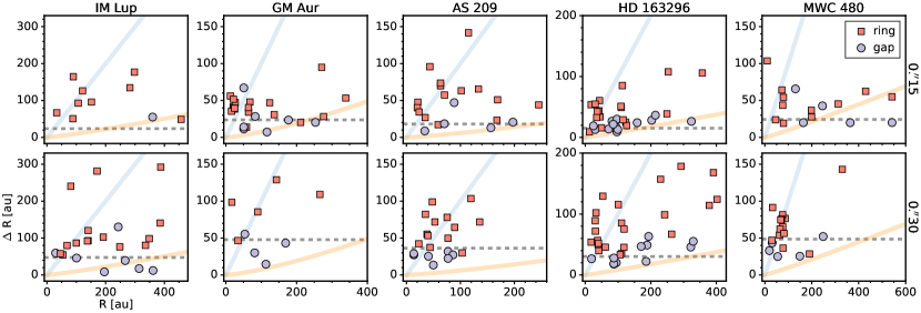
Figure 18: Substructure width as a function of radial location for lines at 0$\farcs$15 (top row) and 0$\farcs$3 (bottom row) resolution. Red squares denote rings and purple circles mark gaps. The gray dashed horizontal lines correspond to $\theta_{\rm{b}}\times d$, which divides resolved features above the line from those that are unresolved or marginally resolved below or at the line. A constant $\Delta R/R=1$ is shown as a solid blue line. The pressure scale height for each disk from Zhang et al. (2021) is shown as a solid orange line.

4.3 Source-specific description of substructures

In addition to considering the aggregate properties of substructures, we briefly summarize the distribution of substructures, including salient trends or notable features, for each MAPS disk below:

4.3.1 IM Lup

IM Lup is the only MAPS source that shows spiral structures in its millimeter continuum (Huang et al., 2018b), but no corresponding spirals are seen in molecular line emission. Among the MAPS disks, IM Lup possesses the largest radial extent (${\sim}$700 au) in CO 2–1, which has been explained by the presence of a photoevaporative wind (Haworth et al., 2017). IM Lup has a unique line emission distribution with a central depression, broad ring-like structure, and plateau of diffuse emission extending out to large radii (${\sim}$600 au) in nearly all lines. This morphology is best illustrated by C₂H 3$-$2 (Figures 4 and 10) and HCN 3$-$2 (Figures 6 and 12) and is also seen, to a lesser degree, in HCO⁺ 1–0 and H₂CO 3–2 (Figures 5 and 11). Plateau-like emission, although at low SNR, is also observed in HCN 1–0 and CN 1–0. DCN 3–2 has a broad double-ringed emission morphology, similar to previous observations of double rings in DCO⁺ 3–2 (Öberg et al., 2015a; Huang et al., 2017) and N₂D⁺ 3–2 (Cataldi et al., 2021). IM Lup has the lowest SNR emission for each line in our sample and is the only disk with non-detected transitions in the set of lines considered here (see Ilee et al. 2021 for more details). As IM Lup is the youngest (0.2–1.3 Myr; Alcalá et al., 2017) MAPS source, the origin of some of these unique features may be a consequence of its youth.

4.3.2 GM Aur

The GM Aur disk is classified as a transitional disk due to its central dust and gas cavity (Calvet et al., 2005; Dutrey et al., 2008; Hughes et al., 2009). Subsequent observations detected inner continuum emission and resolved this dust cavity into an annular gap at 15 au with a corresponding but more compact gas cavity (Huang et al., 2020). The MAPS observations confirm this, as GM Aur has a central dip and bright, compact inner ring at ${\sim}$15–30 au in all lines at 0$\farcs$15 resolution. This is best illustrated by the inner HCN 3–2 and HC₃N 29–28 (Figures 6 and 12) and H₂CO 3–2 (Figures 5 and 11) emission rings. In contrast, the 0$\farcs$3 resolution profiles, e.g., HCN 1–0 and HC₃N 11–10, show a smoothly rising profile in the inner disk. This is likely a resolution effect, and the presence of an inner ring in these lines could be confirmed with higher angular resolution observations. For a more detailed discussion of the inner regions of GM Aur, see Section 5.4. Beyond this inner compact ring, some lines, e.g., HCN 3–2, decrease smoothly with radius, while others such as C₂H 3–2 (Figures 4 and 10) show the presence of two additional, narrow rings (B68, B124). An outer ring at ${\sim}$300 au is seen in HCN 3–2, 1–0; C₂H 3–2; and DCN 3–2, while diffuse emission out to ${\sim}$450 au is present in HCO⁺ 1–0, H₂CO 3–2, and CN 1–0 (Figures 5 and 11). GM Aur also exhibits dramatic spiral arms in CO 2–1 (Figure 3; see Huang et al. (2021) for more details), which are not seen in any other lines in either GM Aur or across the MAPS sample.

4.3.3 AS 209

AS 209 has the most compact MAPS disk, with many lines not extending beyond ${\sim}$200 au and an outer CO 2–1 radius of no more than ${\sim}$300 au. We identify three gaps in CO 2–1, but do not detect the gap at 74 au reported in the higher spatial resolution (0$\farcs$08) observations of Guzmán et al. (2018b). Notably, it is the only MAPS disk with high contrast substructures in its CO isotopologues, namely outer ¹³CO and C¹⁸O emission rings at ${\sim}$120–130 au (Figures 3 and 9), as seen in previous observations (Huang et al., 2016; Favre et al., 2019). These well-defined rings suggest that these lines are less optically thick relative to CO isotopologues at the same radii in other MAPS disks. Thus, the rings and gaps in AS 209 are most likely a result of local variations of CO abundance and gas column density (Alarcón et al., 2021; Zhang et al., 2021). The majority of non-CO lines in AS 209 take the form of a central depression and a broad single ring at ${\sim}$50–80 au, but many lines also exhibit low contrast emission shoulders, e.g., c-C₃H₂ 7–6 (Figure 10); HCO⁺ 1–0, CN 1–0 (Figure 11); and HCN 1–0 (Figure 12). This hints at the presence of additional but unresolved narrow rings. If this single ring is in fact two (or more) narrow rings, this would more closely mirror the continuum structure, which is in the form of a tightly nested set of narrow concentric rings (Guzmán et al., 2018b).

4.3.4 HD 163296

HD 163296 has the largest number of unique substructures among the MAPS disks and shows a well-defined, multi-ringed emission morphology in the majority of lines. Indications of rings seen by Bergner et al. (2019) are now confirmed by the MAPS observations, which show four well-defined rings in HCN 3–2 (Figures 6 and 12) and C₂H 3–2 (Figure 13). Most lines show one (CH₃CN 12–11, HC₃N 29–28, 11–10, CS 2–1), two (c-C₃H₂ 7–6, DCN 3–2), or three (CN 1–0) rings, which are approximately radially coincident. The outermost emission rings in C₂H 3–2, HCN 3–2, 1–0, CN 1–0 occur at large radii ${\sim}$400 au and are the most radially-extended non-CO substructures seen in the MAPS disks. A ring-like feature (B44) is also present in C¹⁸O 2–1 (Figures 3 and 9), while HCO⁺ 1–0 and H₂CO 3–2 (Figures 5 and 11) show blended ring-like structures, some of which had been seen previously in Huang et al. (2017); Carney et al. (2017); Guzmán et al. (2018a).

4.3.5 MWC 480

MWC 480 shows the greatest morphological variations between hydrocarbons and nitriles. C₂H and c-C₃H₂ (Figures 4 and 10) are in the form of a single ring, while HCN and HC₃N (Figures 6 and 12) have centrally peaked profiles with shallow gaps. This latter distribution is unique among non-CO lines across the MAPS disks and is best described as superimposed emission plateaus of different intensities, where the gaps mark the transition regions. DCN 3–2 does not follow this trend and is instead in the form of a single emission ring, similar to C₂H and c-C₃H₂ rather than the other nitriles. A single ring is also evident in HCO⁺ 1–0, H₂CO 3–2, CN 1–0, and CS 2–1 (Figures 5 and 11) and is radially coincident with the hydrocarbon ring. Despite its compact radial extent in most lines, MWC 480 has extended (${\sim}600$ au) and structured CO 2–1 emission in the form of four concentric bright-dark features. Further discussion of the origins and nature of these CO 2–1 substructures is found in Teague et al. (2021).

5 Origins of chemical substructure

The presence of rings, gaps, and other substructures in molecular line emission may be the result of various chemical effects, including variations in C/O ratios, freeze-out onto grains in the disk midplane, thermal desorption in dust substructures, and UV-driven production or selective photodissociation in the disk atmospheres (e.g., Teague et al., 2017; Cazzoletti et al., 2018; Miotello et al., 2019). Substructures can also result from local deviations in disk physical structure, either in density or temperature, e.g., from planet-disk interactions or alterations in dust properties (Bae et al., 2017; Guzmán et al., 2018b; Huang et al., 2020). Non-LTE and excitation effects have a direct effect on observed emission intensities (Pavlyuchenkov et al., 2007). Many of these topics are the subject of other MAPS papers (Aikawa et al., 2021; Alarcón et al., 2021; Bergner et al., 2021; Bosman et al., 2021a; Calahan et al., 2021; Cataldi et al., 2021; Guzmán et al., 2021; Schwarz et al., 2021; Teague et al., 2021; Zhang et al., 2021), while here we instead aim to empirically explore and connect spatial trends in chemical substructures with their potential chemical and physical origins. We also briefly comment on some notable trends and describe those of particular interest in more detail below.

5.1 Spatial links between chemical substructures

We want to assess the relative similarity of molecular line emission profiles within each disk and across the entire MAPS sample. In this context, similarity means consistent radial morphologies, namely the shapes and locations of gaps, rings, and emission shoulders. To quantify this kind of similarity, we compared pairs of radial profiles and calculated their radially-integrated absolute differences. The profiles were first normalized such that the peak brightness of the first profile (corresponding to the line with the brighter absolute peak intensity) was set to unity, and then the second radial profile was scaled to minimize the difference between the two profiles. We found that this approach is effective at identifying profiles that look similar by eye, i.e., it does not overly penalize profiles with different relative fluxes but otherwise similar morphologies, such as HCN 3–2 and DCN 3–2 or HCN 3–2 and C₂H 3–2 in HD 163296.

Figure 19 shows the results for all pairs of lines in each disk. Pairs of lines with profiles that are more dissimilar in their emission morphologies are shown in darker colors, while those that are more similar are shown in lighter colors. To acknowledge the semi-qualitative nature of this comparison we only use four colors, corresponding to four quartiles of similarity. Overall, this method, while not intended to provide a robust statistical measure, allows for a useful ordering based on the similarity of line pairs.

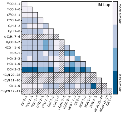
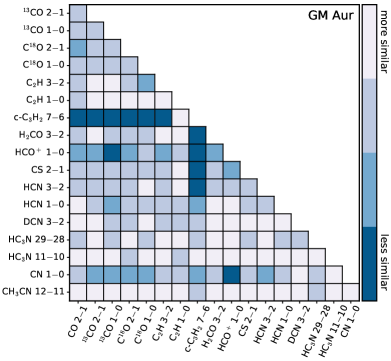
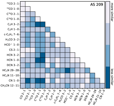
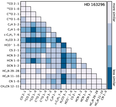
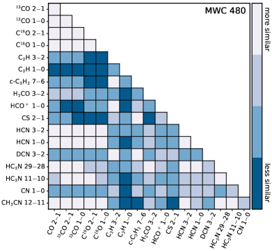
Figure 19: Integrated differences between all pairs of lines within each MAPS disk. Darker colors indicate lines with less similar radial morphologies, while lighter colors show those that are more similar. Hatched squares designate tentative and non-detected lines, or those lacking sufficient SNR for a robust comparison.

IM Lup has the highest fraction of line pairs with similar morphologies, with most lines showing a central depression, followed by a wide ring and plateau-like distribution. GM Aur, AS 209, and HD 163296 also show a relatively large fraction of similar lines. This is due to the consistent emission structures within each disk, namely a central cavity and narrow inner ring (GM Aur); a single emission ring (AS 209); and multiple co-spatial rings of comparable widths (HD 163296). In contrast, MWC 480 shows the most dissimilar line pairs, which reflects broad differences in radial morphologies between different types of species. For instance, the hydrocarbons are in the form of a single ring with a central gap, while the CO lines and HCN 3–2 and HC₃N 29–28 have smoothly-decreasing, centrally-peaked profiles. In several disks, we also find that one or two lines are markedly different from the others: DCN 3–2 in IM Lup, c-C₃H₂ 7–6 in GM Aur, and H₂CO 3–2 in HD 163296. These differences reflect the mutually dissimilar emission structures of each line, i.e., double rings (DCN 3–2), a radially-offset emission ring (c-C₃H₂ 7–6), and a large central gap (H₂CO 3–2).

Within each disk, the CO isotopologues are the mutually most consistent, which is not surprising considering all lines originate from the same species, but yet informative since it suggests that excitation and optical depth effects do not dominate differences in radial profiles. Species belonging to the same molecular families, e.g., C₂H and c-C₃H₂; HCN and HC₃N, as well as different transitions from a single species, e.g., C₂H 3–2, 1–0; HCN 3–2, 1–0, are also typically similar to one another. This is an intuitive result since the radial profiles appear similar, with consistent multi-ring emission structures, e.g., C₂H and c-C₃H₂ in HD 163296 (Figure 10), or emission shoulders that occur at similar radial locations, e.g., double shoulders in HCN 3–2 and HC₃N 29–28 in MWC 480 (Figure 12). As for the CO isotopologues, this broad similarity in the radial profiles of similar molecules or different transitions of the same species indicates that excitation effects are not causing substantial differences in their radial morphologies. This is unsurprising as typical differences in upper state energies are only a few 10s of K, with the exception of HC₃N 29–28 (E${}_{\rm{u}}~{}\approx$ 190 K).

Overall, the correlation patterns between the five disks appear quite complex. A few lines are consistently well-correlated, but many aspects of disk chemistry are disk specific. For instance, the relationship between HCN and H₂CO spans from strongly dissimilar in HD 163296 to strongly similar in IM Lup and GM Aur with only a modest association in AS 209 and MWC 480, while C₂H and CO lines are well-correlated in IM Lup and GM Aur, but are dissimilar in AS 209, HD 163296, and MWC 480.

5.2 Relationship between chemical and continuum substructures

One primary goal of this work is to assess the relationship between continuum and chemical substructures at high spatial resolution in protoplanetary disks. Figure 20 shows the radial locations of chemical substructures versus those of annular continuum substructures in the MAPS disks. Although there is no one-to-one correlation between continuum and line emission substructures, several suggestive trends emerge. Below, we first provide a source-by-source description in Subsection 5.2.1. Then, in Subsection 5.2.2, we discuss the spatial links between dust and chemical substructures across the entire MAPS sample as well as comment on the relative frequency of such associations and likely physical origins. In Subsection 5.2.3, we identify and discuss molecular emission features that are coincident with the outer edge of the millimeter continuum disks.

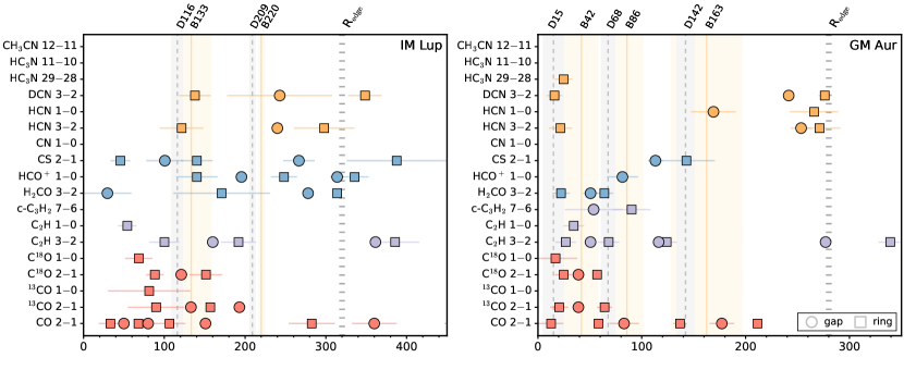
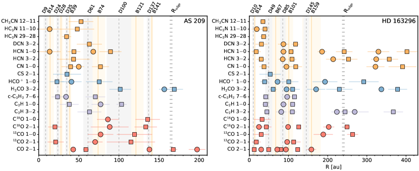
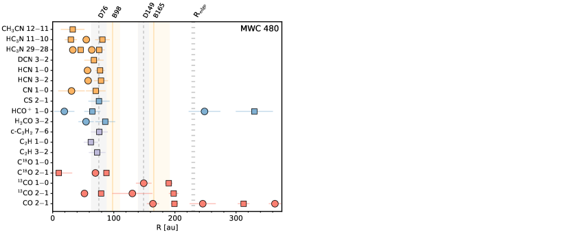
Figure 20: Radial locations of chemical and millimeter continuum substructures in the MAPS sample. Line emission rings and gaps are shown as squares and circles, respectively. Species are color-coded, as in Figures 15, 16, and 17. Gray dashed lines mark continuum gaps and orange solid lines denote continuum rings. Shading indicates the widths of continuum substructures. All millimeter continuum features are labeled according to Table 5. Broad dotted lines mark the location of the edge of millimeter continuum disk. Chemical substructures at large radii beyond the millimeter continuum, which are only seen in CO 2–1, are omitted. The widths of error bars for chemical substructures represent $\sigma$ instead of the full FWHM, i.e., FWHM / 2.355, for visual clarity.

5.2.1 Source-specific trends

In IM Lup, a few line emission rings, e.g., ¹³CO 2–1, HCN 3–2, DCN 3–2, HCO⁺ 1–0, are coincident with the inner continuum ring (B133). However, the majority of chemical substructures are widely distributed in radial locations with no particular association with continuum substructures. A few chemical substructures (e.g., HCN 3–2, DCN 3–2, H₂CO 3–2) at larger radii are spatially associated with the outer edge of the continuum disk.

In GM Aur, chemical substructures are closely associated with the inner three continuum features (D15, B42, D68). Specifically, we see alternating pairs of ring-gap associations between the continuum and chemical substructures: line emission rings are associated with the D15 dust gap, line emission gaps with the dust gap at B42, and another set of line emission rings at the dust gap at D68. Few chemical substructures are present beyond ${\sim}$120 au with the notable exception of a set of outer emission rings in HCN 3–2, 1–0, and DCN 3–2, each of which are coincident with the outer continuum edge.

In AS 209, the majority of chemical substructures are spatially coincident with continuum substructures. The inner line emission gaps in HCN 1–0 and HC₃N 11–10 are both radially coincident with the B14 dust ring. Line emission peaks in ¹³CO 2–1, C¹⁸O 2–1, c-C₃H₂ 7–6, HCO⁺ 1–0 are aligned with the D24 dust gap and CS 2–1, CN 1–0, and HC₃N 29–28 rings aligned with the D35 dust gap. Similarly, several emission rings (c-C₃H₂, HCO⁺, CN) are located near the dust ring at B74. However, not all line substructures are aligned with continuum substructures. Several nitrile rings (HCN 3–2, 1–0, CH₃CN 12–11, HC₃N 11-10) fall between the dust ring at B39 and dust gap at D61. Interesting, there are relatively few chemical substructures within the broad D100 dust gap. No chemical substructures, with the exception of CO 2–1, are located beyond the continuum edge.

In HD 163296, nearly all chemical substructures show some spatial association with those of the continuum within ${\sim}$120 au, while few features are associated with the outer dust ring-gap pair (D145-B159). Chemical rings and gaps within 120 au are also radially coincident with one another. This consistency in radial location is particularly striking for those substructures associated with the hydrocarbons and nitriles. Line emission rings are coincident with the dust gap at D49, while gaps in line emission are coincident with the dust gap at D85. Another set of chemical rings aligns with the B101 dust ring. Over 20% — the highest fraction in the MAPS disks — of chemical substructures are located at or beyond the edge of the millimeter continuum disk.

In MWC 480, the majority of chemical substructures are radially coincident with the D76 dust gap with line emission rings showing the closest spatial associations. However, in some cases, e.g., HC₃N 29–28, line emission rings and gaps both overlap within the width of the D76 dust gap. Besides CO isotopologues and HCO⁺, no other chemical substructures are seen outside of the inner D76-B98 continuum feature. The numerous CO substructures at large radii generally do not show any trends with continuum features with the exception of CO 2–1, ¹³CO 2–1, 1–0 rings around 200 au, which is at the outer edge of the B165 dust ring.

5.2.2 Spatial links between chemical and dust substructures across MAPS disks

While, in detail, each disk displays a different relationship between chemical and continuum substructures, several broader trends emerge. Most notably, the majority of chemical substructures across the MAPS disks show some degree of spatial association with continuum substructures for radii less than ${\sim}$100-150 au. Beyond these radii, the fraction of chemical substructures that can be linked to dust substructures is quite small. Chemical substructures in some lines are also present at or near the outer continuum edge in several disks, which is discussed in detail in the following subsection.

To quantify how likely continuum and chemical substructures are to spatially correlate with one another, we calculated the relative occurrence rate of overlapping features. We considered features to be overlapping if the radial position of the chemical substructure (listed in Table 3) falls within the width of the continuum substructure. As the outer continuum ring-gap pair (D209-B220) in IM Lup was visually-identified, we adopt a conservative width of ${\sim}$10 au for both of these features. Figure 21 shows the spatial overlap fractions for all four possible pairs of substructure alignments. The top panel shows the overlap fractions for all chemical substructures. The highest fractions (up to ${\sim}$65%) are between line emission rings-dust gaps and chemical gaps-dust rings, followed by chemical rings-dust rings (${\sim}$10-25%). Chemical gap-dust gap alignments are consistently the least common ($\lesssim$25%). The disk-to-disk variation is high for gap-ring alignments, while ring-ring and gap-gap alignment frequencies are almost constant among the disks.GM Aur shows the highest fractions of overlapping features, which is, in part, due to most species showing emission peaks in its central dust cavity. High overlap fractions are also seen in the MWC 480 disk due to the spatial association of many of its chemical substructures with the continuum gap at D76.

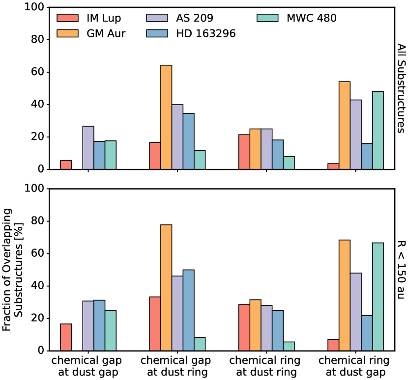
Figure 21: Fraction of chemical and millimeter continuum substructures that spatially overlap for all chemical structures (top) and those with radial locations ${<}$150 au (bottom). Overlapping features are those where the radial location of a line emission substructure falls within the width of a continuum feature.

The bottom panel of Figure 21 only considers those chemical substructures with radial locations less than 150 au, which yields 10–20% higher overlap fractions for nearly all disks and substructure alignments. For instance, all disks have over one-third of either (or both) chemical rings and dust gaps or chemical gaps and dust rings aligned in the inner 150 au. GM Aur and MWC 480 chemical ring-dust gap alignments are ${\sim}$70%. Thus, in general, chemical and dust substructures are closely associated in the inner 150 au of disks.

Dust gaps may cause chemical gaps if they are associated with gas depletion. Similarly, dust rings may result in chemical rings if they are associated with gas enhancements. Dust gaps and rings may also give rise to either chemical gaps or rings due to changes in radiation, ionization, gas-phase elemental abundances, and temperature, since different species are expected to be more rapidly formed or destroyed as these properties increase or decrease (e.g., Facchini et al., 2018; Alarcón et al., 2020; Rab et al., 2020). However, many associations between line emission and continuum features are independent of gas-dust substructure correlations, i.e., only some dust gaps are obviously also depleted in gas (Zhang et al., 2021). For these cases, some process is needed to link the midplane and elevated disk layers, since millimeter dust grains emit from near the midplane (e.g., Villenave et al., 2020) and line emission from vertically flared surfaces (e.g, Podio et al., 2020; Teague & Loomis, 2020b; van’t Hoff et al., 2020; Law et al., 2021).

Such links may be due to vertical mixing (Semenov & Wiebe, 2011; Flock et al., 2017; van der Marel et al., 2021) or flows of molecular material from the disk surface to the midplane at the radial locations of dust gaps (Teague et al., 2019). Theoretically, these links should be easier to establish in the inner disk regions, since most line emission heights are expected to increase with radius due to disk flaring. Moreover, dust scale heights may also be locally-enhanced, i.e., comparable to that of the gas (Doi & Kataoka, 2021), in the inner disk, which would place the line and dust emitting regions in closer contact. This provides a natural explanation for the frequent dust and line emission associations seen within 150 au, but the relatively few at larger radii, at which point the increasingly flared surfaces become disconnected from disk midplanes. We would also expect a closer association between dust and those molecules, that for chemical or excitation reasons, emit closer to the midplane. In general, disks are expected to be highly stratified with different lines and species originating in different vertical layers (Dartois et al., 2003), and thus different lines may become disconnected from the midplane dust at different radii depending on their particular emission heights.

In the case of chemical gap-dust ring association there is also another possible explanation: the absorption of line emission by dust. Continuum subtraction of the dust emission may result in gaps in molecular line emission in regions where the line emission is optically thick and absorbs most of the dust emission coming from the midplane (e.g., Boehler et al., 2017; Weaver et al., 2018). While this may be responsible for some of the observed spatial links, especially in the inner 50 au, the lack of consistent associations between line emission and dust substructure suggests that this is not a dominant effect. For instance, in HD 163296, one set of line emission rings aligns with the D49 dust gap, while another group of chemical rings is co-located with the B101 dust ring.

While gas and millimeter dust emit from distinct disk layers, gas emitting surfaces and dust scattered light features are, in some cases, vertically co-located (see Law et al., 2021). As IM Lup, AS 209, and HD 163296 also have well-defined rings in scattered light (Monnier et al., 2017; Muro-Arena et al., 2018; Avenhaus et al., 2018; Rich et al., 2020), we searched for spatial associations between chemical substructures and these NIR rings. We found no strong links with the following two exceptions. The outermost set of gaps in CN 1–0, HCN 3–2, 1–0 in HD 163296 are approximately aligned with the NIR ring at 330 au (Rich et al., 2020). In IM Lup, the NIR ring at 240 au (Avenhaus et al., 2018) is co-located with a gap in HCN 3–2 and the center of the large gap between the double DCN rings. These spatial associations are intriguing, as NIR wavelengths probe micron-sized grains in elevated disk layers that help regulate UV flux, which is an important parameter for the formation of CN and HCN. A more detailed discussion of NIR features and these two molecules in the MAPS disks is found in Bergner et al. (2021). Figure 31 in Appendix G shows the full comparison between chemical substructures and NIR rings in these three disks.

5.2.3 Outer edge of millimeter continuum disk

Line emission features are often spatially associated with the edge of the millimeter continuum in disks (e.g., Öberg et al., 2015a; Bergin et al., 2016). In particular, associations between line emission rings and continuum edges have been previously observed in the MAPS disks, e.g., for DCO⁺ in IM Lup (Öberg et al., 2015a; Huang et al., 2017) and HD 163296 (Salinas et al., 2017; Flaherty et al., 2017); H¹³CO⁺ (Huang et al., 2017) and H₂CO (Carney et al., 2017) in HD 163296, as well as for ¹³CO (Schwarz et al., 2016) and C₂H (Bergin et al., 2016) in TW Hya; HCN (Guzmán et al., 2015) and C₂H (Bergin et al., 2016) in DM Tau; and DCN in LkCa 15 (Huang et al., 2017). The MAPS data also show that an N₂D⁺ 3–2 emission ring in IM Lup, AS 209, and HD 163296 is associated with the outer continuum edge (Cataldi et al., 2021). Models explain these spatial links in the context of dust evolution leading to non-thermal desorption (Öberg et al., 2015a), a thermal inversion in the outer disk (Cleeves, 2016; Facchini et al., 2017), or higher UV penetration at this dust edge (Bergin et al., 2016). To explore links between chemical substructure and disk edges, we first visually estimate the outer edge of the millimeter continuum R_edge for each disk from the radial profiles in Figure 14. The determined R_edge values are listed in Table 5 and are shown as broad dotted lines in Figure 20.

We observe coincidences between R_edge and line emission rings in all MAPS sources except MWC 480. Rings from HCN and DCN in GM Aur, IM Lup, and HD 163296 are spatially correlated with R_edge, as are H₂CO rings in IM Lup, AS 209, and HD 163296. In fact, when combined with the previous survey of Pegues et al. (2020), these results indicate that at least 50% of disks may show spatial associations between H₂CO rings and continuum edges (see Guzmán et al., 2021, for further details). Moreover, this also suggests that similar fractions of HCN and DCN rings may be spatially linked to R_edge, but this requires a large disk survey at high spatial resolution and sensitivity to confirm.

HCN, DCN, and H₂CO are not directly chemically linked, and their joint appearance at the edge of the pebble disk suggests that some or perhaps all of the proposed chemical effects listed above are active at different levels in the different disks. HCN and DCN are expected to form through gas-phase chemistry, and the origins of the HCN and DCN line emission rings are likely due to higher UV penetration at the dust edge increasing the atomic carbon abundance (Alarcón et al., 2020). One potential caveat of this explanation is that we never observe a corresponding association between a ring in the photochemically sensitive CN molecule and R_edge, but this may also be explained by CN emission originating from elevated disk layers (Cazzoletti et al., 2018; Teague & Loomis, 2020b; Bergner et al., 2021). H₂CO may form in the gas-phase or through grain-surface chemistry via CO ice hydrogenation (e.g., Loomis et al., 2015). At the millimeter dust edge, H₂CO could arise from either non-thermal desorption of H₂CO ice, or by gas-phase formation following thermal or non-thermal CO desorption, or by gas-phase formation fuelled by photo-produced atomic carbon (Qi et al., 2013; Öberg et al., 2017; Pegues et al., 2020; Terwisscha van Scheltinga et al., 2021). In disks where the HCN and H₂CO rings coincide, the latter seems the most likely explanation. By contrast, in the IM Lup disk, the proximity of HCO⁺, DCO⁺, and DCN rings to R_edge, indicates that in this case the edge of the pebble disk results in cold CO-driven chemistry, as well as an increased ionization rate, and an increased gas-phase deuteration chemistry.

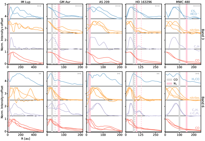
Figure 22: Normalized radial intensity profiles for lines observed in Band 3 (top) and Band 6 (bottom). In the case of Band 6, most lines are at 0$\farcs$15, but some are tapered to 0$\farcs$30 (see Table 1). Each panel is subdivided by species and vertically offset for visual clarity. Species are color-coded, as in Figures 15, 16, and 17. Shading shows the radial range of the CO (gray) and N₂ (pink) midplane snowlines derived with thermochemical models (Zhang et al., 2021), while the dashed lines indicate those determined from observations of N₂H⁺ (Qi et al., 2015, 2019). Only the central radius of the N₂H⁺-derived snowlines are shown and uncertainties are omitted for visual clarity but are typically on the order of 5–10 au. The FWHM of the synthesized beam is shown by a horizontal bar in the upper right corner of each panel.

In summary, given the diversity in spatial associations with the outer disk edge across the MAPS disks, no single explanation can account for these trends. Instead, some combination of different processes must be at work and their relative importance appears to depend on the specific physical conditions of each disk.

5.3 Relationship between chemical substructures and snowlines

The condensation of key volatiles, such as CO₂, CO, and N₂, has been suggested as one possible origin for annular continuum substructures due to changes in the fragmentation and coagulation properties of dust grains at the location of molecular snowlines (e.g., Zhang et al., 2015; Okuzumi et al., 2016). The freezeout of different volatiles will also lead to changes in elemental and molecular composition in disks that may generate, or facilitate the growth of, chemical substructures at or near the location of particular snowlines. To explore whether the chemical substructures observed in MAPS are connected to molecular snowlines, we first show the normalized radial profiles of all lines considered in this study in Figure 22. We then shade the radial locations of the midplane snowlines of CO (gray) and N₂ (pink) derived from the thermochemical models of Zhang et al. (2021). Snowlines determined using observations of N₂H⁺ from Qi et al. (2015, 2019) are indicated as dashed lines but are only available for GM Aur (CO and N₂) and HD 163296 (CO). The MAPS observations of N₂H⁺ 3–2 and N₂D⁺ 3–2 (e.g., Aikawa et al., 2021; Cataldi et al., 2021) suggest that the N₂ snowline in HD 163296 is at approximately 130 au (Qi, private comm.). In all MAPS disks, the CO₂ snowline occurs at a radius of ${<}$10 au from the central star (Zhang et al., 2021) and is thus always unresolved.

No strong spatial association between the locations of chemical substructures and snowlines is evident in Figure 22. Moreover, there also are no obvious trends in the relative locations of chemical substructures and snowlines. For instance, nearly all line emission substructures in IM Lup and AS 209 are at radii exterior to the CO and N₂ snowlines, while the majority of features in MWC 480 are located interior to both snowlines. GM Aur and HD 163296 show a more widely spread distribution of substructures that occur across snowlines.

A few tentative associations are seen within individual disks, such as the alignment of the CO snowline with the edge of the central depression in IM Lup or several line emission rings (C₂H 3–2, H₂CO 3–2) that are radially coincident with the N₂ snowline in GM Aur. However, the relative uncertainty in snowline locations often makes discerning precise spatial links difficult. For example, in GM Aur, the CO snowline from the models of Zhang et al. (2021) is at 30 au, which is radially coincident with line emission rings (CO, HCN, C₂H, H₂CO), but the CO snowline predicted from N₂H⁺ (Qi et al., 2015) is at 48 au which instead is spatially co-located with several line emission gaps (H₂CO, C₂H, c-C₃H₂). A similar discrepancy is seen in HD 163296 with the N₂ snowline from Zhang et al. (2021) aligning with chemical gaps, while the snowline based on N₂H⁺ aligns, or is slightly exterior to, several chemical rings. More empirical data on the snowline locations of CO and N₂ are needed to derive reliable statistics on links between snowlines and the locations of either chemical or dust substructures. However, even for the cases where snowline estimates based on N₂H⁺ exist, at most a small fraction of chemical substructures are spatially coincident and therefore possibly caused by snowlines.

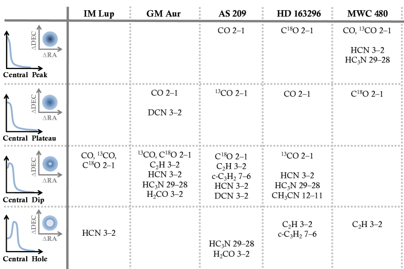
Figure 23: Grid of radial morphologies in the inner 50 au of the MAPS disks. The rows classify lines by the shape of the central emission. Classifications are restricted to those lines observed in Band 6 and are based on the normalized intensity at the innermost radial bin in the radial profiles according to: I${}_{\rm{norm}}{<}$0.2 (hole), 0.2$<$I${}_{\rm{norm}}<$0.8 (dip), I${}_{\rm{norm}}{>}$0.8 (peak or plateau). The difference between a peak and plateau was determined visually. Grid adopted and lightly modified from Pegues et al. (2020).

Thus, snowlines do not offer a universal explanation for the observed chemical substructures. However, this does not rule out that 2D snow-surfaces play a more important role in regulating disk chemical structures. Emission from molecular lines in disks often originates from an elevated emitting surface. A potentially informative, but intensive comparison would involve a 2D disk-specific model for each snow surface of interest and a diverse set of molecules with well-constrained emission surfaces.

5.4 Line emission at ${<}$50 au

The high angular resolution of the MAPS observations provides access to the behavior of gas in the inner 50 au, which is directly relevant for the formation of planets, such as the giant planets in our own solar system. Here, we explore trends in line emission within this inner region, while Bosman et al. (2021b) provides a more detailed and quantitative examination of the CO lines within the innermost 20 au. We only consider those lines covered in Band 6, as they possess the highest angular resolutions (0$\farcs$15). We omitted those lines, although covered in Band 6, that required the use of the tapered images to achieve sufficient SNR (see Table 1). In Figure 23, we adopted the qualitative grid employed by Pegues et al. (2020) and classified radial morphologies by normalized intensities at the innermost radial bins of the radial profiles according to: I${}_{\rm{norm}}{<}$0.2 (hole), 0.2$<$I${}_{\rm{norm}}<$0.8 (dip), I${}_{\rm{norm}}{>}$0.8 (peak or plateau). The difference between a peak and plateau was determined visually.

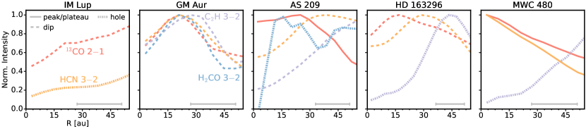
Figure 24: Normalized radial intensity profiles of select lines covered in Band 6 at 0$\farcs$15 in the inner 50 au. Species are color-coded, as in Figures 15, 16, 17, 22. Classifications, as in Figure 23, of central peaks/plateaus, dips, and holes are shown as solid, dashed, and dotted lines, respectively. The FWHM of the synthesized beam is shown by a horizontal bar in the lower right corner of each panel.

Figure 23 shows that there is a wide range of radial morphologies within 50 au in different disks and lines. This is further illustrated in Figure 24, which shows normalized radial profiles for representative lines in each disk. For instance, the majority of lines in GM Aur show a central dip and are remarkably consistent in their central radial behavior, while AS 209 and HD 163296 have lines that exhibit all possible central behaviors from dips to peaks. MWC 480 has the highest fraction of lines showing a central peak. IM Lup consistently shows a central dip or hole, but as only HCN 3–2 and the 2–1 transitions of the CO isotopologues had sufficient SNR at 0$\farcs$15, conclusions are necessarily limited. We note, however, that the majority of lines at 0$\farcs$30 in IM Lup also show evidence of a central depression and as this central deficit has a large radial extent ($\gtrsim$100 au), it is resolved even at 0$\farcs$30 for many lines, e.g., C₂H 3–2, HCO⁺ 1–0.

Figure 24 shows that if we survey a single disk in different lines, we often see a diversity of line emission profiles within the central 50 au. In MWC 480, for example, C₂H 3–2 steadily decreases in the form of a central hole, while both CO 2–1 and HCN 3–2 are centrally peaked. Similar species-specific differences are also present in AS 209 and HD 163296. If we survey all of the disks in a single line, we also see a diversity in radial morphologies. For instance, HCN 3–2 spans the range of possible central behaviors with a central peak in MWC 480, central dip in GM Aur, AS 209, and HD 163296, and central hole in IM Lup. Thus, the chemistry appears quite different between disks, which implies both that planets may assemble in chemically distinct environments when forming at the same radius around different stars, and that common molecular probes may trace different regions in different disks.

The most common type of central behavior across lines and disks is that of a central dip. One reason for this may be the dust optical depth. As the dust becomes modestly optically thick interior to ${\sim}$30 au in IM Lup, HD 163296, and MWC 480, and possibly in AS 209, (Sierra et al., 2021), we expect a reduction in intensity as the back side of the disk is increasingly hidden. However, this cannot fully explain the observed diversity in radial morphologies, as dust optical depth would block the back side of the disk leading to only a factor of two reduction (unless the scale height of the millimeter grains is higher as suggested in IM Lup by Bosman et al. (2021b)). Instead, these features are likely due to a combination of differences in abundance, excitation, temperature, and chemistry in the inner regions of the MAPS disks.

The only non-CO molecules to show either central peaks or plateaus in their radial morphologies are nitriles. In particular, MWC 480 shows sharply-rising HCN and HC₃N profiles, while DCN 3–2 is in the form of a central plateau in GM Aur. Nitriles may be important players in origins of life chemistry (Powner et al., 2009; Sutherland, 2016) and it is interesting that, at least in some cases, nitriles peak toward the innermost regions of planet-forming disks. Indications that HCN emits from a surface relatively close to the disk midplane (Law et al., 2021) further suggest a potential connection to planet-forming material.

6 Summary

We present a systematic analysis of radial substructures in a set of 18 molecular emission lines toward five protoplanetary disks observed at high angular resolution as part of the MAPS Large Program. We conclude the following:

1. Over 200 unique radial chemical substructures, including rings, gaps, and emission plateaus, are identified. Substructures occur at nearly all radii where line emission is detected with widths ranging from ${<}$10 au to over 200 au.

2. All lines are azimuthally symmetric, at least to first order, with the exception of the spiral arms seen in CO 2–1 in GM Aur. This is true even for those disks that have millimeter continua with known non-axisymmetric features (HD 163296) or spiral arms (IM Lup).

3. The large radial extent of CO and its inorganic and organic derivatives compared to O-poor molecules, such as the hydrocarbons C₂H, c-C₃H₂ and nitriles HC₃N, CH₃CN, indicates that the inner planet-forming 100 au of disks may be more C-rich than disk-averaged line emission suggests. Additionally, the complex nitriles and c-C₃H₂ are spatially compact and do not extend beyond the edge of the continuum disk. At radii beyond the pebble disk, these molecules may be more easily destroyed, e.g., due to radiation or increased gas-phase O-chemistry.

4. Within 150 au, there is substantial spatial overlap between dust and chemical substructures, while in the outer disks, such overlaps are sparse. This suggests a scenario where the dust-emitting midplane and warm molecular layers are linked in the inner disk regions but become increasingly disconnected at larger disk radii.

5. Some chemical substructures are spatially associated with the outer edge of the millimeter continuum. In particular, HCN, DCN, and H₂CO emission rings are commonly coincident with the outer continuum edge in the MAPS disks.

6. The vast majority of chemical substructures in the MAPS disks are not spatially associated with midplane snowlines, which indicates that snowlines do not directly cause most chemical substructures.

7. In the inner 50 au, the MAPS disks exhibit a wide range of radial morphologies, including central peaks, plateaus, dips, and holes. This diversity is present both across disks and between lines, where it is often but not exclusively associated with molecules of different chemical families. The only non-CO molecules to show central peaked profiles are those of the nitriles HCN, HC₃N, and DCN.

The MAPS observations reveal a striking diversity in the radial morphologies of molecular line emission in protoplanetary disks. Chemical substructures are ubiquitous and extremely varied with a wide range of radial locations, widths, and relative contrasts. This suggests that planets often form in diverse chemical environments both across disks and at different radii within the same disk. While the MAPS Large Program provides a comprehensive view of the chemical environments in which planet formation occurs, the observations are of a sample of only five carefully-selected disks. Unbiased surveys toward larger numbers of disks at comparably high spatial resolution are required to determine the universality of the trends identified here and to assess if typical planet-forming disks host chemical environments similar to those of the MAPS disks.

7 Value-Added Data Products

The MAPS Value-Added Data Products described in this work can be accessed through the ALMA Archive via https://almascience.nrao.edu/alma-data/lp/maps. An interactive browser for this repository is also available on the MAPS project homepage at http://www.alma-maps.info.

For each combination of transition (Tables 2 & 3, Oberg et al., 2021), disk (Table 1, Oberg et al., 2021), and spatial resolution (Table 5, Oberg et al., 2021), the following data products are available:

• Zeroth moment map

• Rotation map

• Peak intensity map

• Radial intensity profile (including a combination of wedge sizes and with surfaces, when available)

• Emission surface, when available (see Law et al., 2021, for more details)

• Python script to generate the data products

For VADPs generated using bettermoments, namely the zeroth moment, rotation, and peak intensity maps, we also provide the corresponding uncertainty maps. For more information on the data products associated with the imaging process, see Section 9 in Czekala et al. (2021). For a detailed description of the naming conventions of all VADPs, see Section 3.5 in Oberg et al. (2021).

Appendix A Generation of Hybrid Zeroth Moment Maps

Collapsing a three dimensional data cube into a two dimensional moment map requires the loss of information. In this process, the level of masking applied to the data prior to the collapse to the desired summary statistic will largely depend on its desired use.

The most typical mask used is a $\sigma$-clip, which removes all pixels from each channel of the data cube which are below a certain threshold value, e.g., a $2\sigma$ clip where $\sigma$ is the RMS of the cube. While this yields a relatively noise-free moment map, it can significantly reduce the measured integrated intensities. This is especially problematic if a large fraction of emission is expected at a per channel level of $\lesssim 2\sigma$, as is the case for many lines covered by MAPS. Thus, while $\sigma$-clipped moment maps are adequate for qualitative descriptions of emission morphology, they cannot be used for quantitative comparisons.

An alternative approach is to adopt a Keplerian mask (e.g., Rosenfeld et al., 2013; Loomis et al., 2015; Öberg et al., 2015b). For a source in Keplerian rotation, such as the gas in protoplanetary disks, the expected emission morphology is well characterized in position-position-velocity (PPV) space. Using a simple analytical model describing this rotation, it is possible to consider only regions of the cube where line emission should originate and thus avoid unknowingly removing low-level emission. These masks are also routinely used for CLEANing data (see, e.g., Czekala et al., 2021). The use of a sufficiently conservative mask, i.e., one that encloses all disk emission, provides the most accurate description of the integrated intensity. For this reason, we use the Keplerian CLEAN masks from Czekala et al. (2021) when collapsing the data cubes into zeroth moment maps. We use these maps for all quantitative work within MAPS, such as the radial profiles described in this work.

While this approach produced maps with the most accurate flux values, they do not always produce maps that are trivial to interpret visually. For weak lines, this Keplerian masking led to noise-dominated moment maps, primarily because the masks were purposely made large in position-position space, so as not to miss any emission. In addition, artifacts in the form of arc-shaped ridges were present in the central few arcsecs of the maps due to the extended velocity wings required for the CLEAN masks to fully capture ¹³CO emission in the inner disk (Czekala et al., 2021; Bosman et al., 2021b). These features were due to these disk inner regions including a considerably larger number of channels (e.g., see Figure 2) in the integration and thus producing stepped emission distributions.

To account for this, we generated a set of “hybrid” zeroth moment maps using a combination of these techniques: we combined a Keplerian mask with a smoothed, intensity-threshold map, as demonstrated in Figure 25. The top row shows HCO⁺ 1–0 emission in the HD 163296 disk. The second row shows the Keplerian mask used for cleaning. Clearly, this follows the same morphology as the emission in the PPV space of the cube, but overestimates the radial and azimuthal extent of the emission in any given channel. The third row shows a mask based on a $2\sigma$ threshold. While this does a better job of tracing the emission in each channel, it simultaneously misses the low level emission at the edges of the line, while also adding in background noise at large radii. The fourth row shows an extended clip mask, which was generated by convolving the data with a circular Gaussian kernel with a FWHM equal to that of the synthesized beam before the 2$\sigma$ clip was applied to the smoothed data. Applying the $\sigma$-clip to smoothed data has the following benefits: (1) the convolution removes noise peaks at large offsets from the disk center; and (2) where the emission is strong (i.e., values much larger than the adopted clip-threshold), the resultant mask is broader than one generated from the un-smoothed data. This leverages the proximity to real (strong) emission to allow for weaker emission to be included in the moment map which would typically be lost with a $\sigma$-clip. The bottom row shows the final mask, which is a combination of the Keplerian and smoothed $2\sigma$ masks, which together, removes persistent patches of background noise on the scale of the beam.

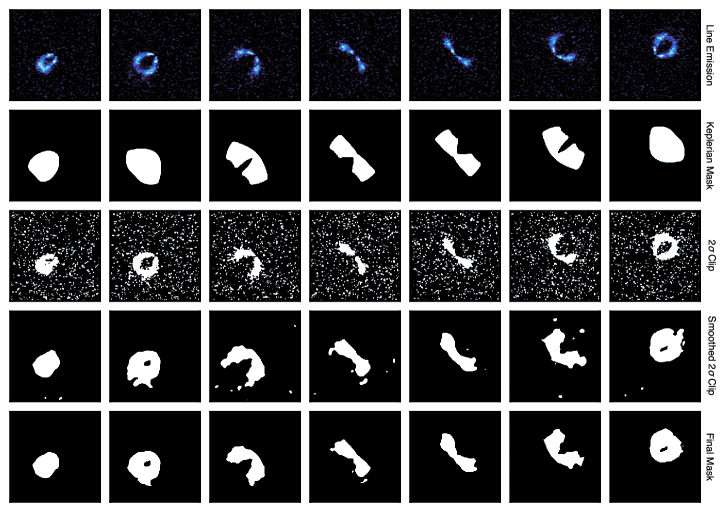
Figure 25: Comparisons of the observed HCO⁺ 1–0 emission from the CLEANed images (top row) in HD 163296 with four types of masks: the Keplerian mask (second row); a threshold mask clipping all values below $2\sigma$ (third row); the threshold mask enlarged by first convolving the emission with a 2D Gaussian kernel based on the synthesized beam before applying the $2\sigma$ clip (fourth row); and the combination of the Keplerian and smoothed $2\sigma$ clip masks (bottom row).

For all lines, disks, and spatial resolutions covered in MAPS (Oberg et al., 2021), we generated hybrid zeroth moment maps with a set of $\sigma$ clips: 0, 0.5, 1.0, 1.5, and 2.0. For each map, we visually selected the lowest clip value that best mitigated the arc-like artifacts, while not substantially lowering the flux. Figure 26 illustrates this process for CS 2–1 in HD 163296. Circular artifacts are evident in the unclipped, Keplerian masked zeroth moment map, as well as in the hybrid maps with $\sigma$ clips of 0 and 0.5. However, the higher $\sigma$ clips of 1.5 and 2 substantially reduce the faint emission in the inner disk, which causes the inner dip in line emission to appear artificially radially extended. In this case, a choice of $\sigma$=1.0 shows an optimal balance between mitigating the central artifacts and retaining sufficient flux to accurately illustrate the spatial distribution of CS 2–1 emission.

To generate these maps, we used the following commands with bettermoments (Teague & Foreman-Mackey, 2018): “bettermoments cube.fits -method zeroth -mask cube.mask.fits -clip -100 X -smooth 3 -smooththreshold 1”, where X is the value of the $\sigma$ clip.

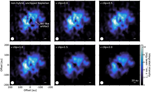
Figure 26: Comparison of unclipped, Keplerian masked zeroth moment map with hybrid zeroth moment maps using different sigma clips for CS 2–1 in HD 163296. The color bar is the same for all panels. The synthesized beam and a scale bar indicating 20 au is shown in the lower left and right corner, respectively, of each panel.

Appendix B Disk-specific zeroth moment map

To illustrate the diversity of radial emission morphologies within each MAPS disk, Figure 27.1 shows a gallery of zeroth moment maps for all 18 lines considered in this study, along with the 90 GHz and 260 GHz continuum images, for the IM Lup disk. A complete gallery of zeroth moment maps for all MAPS disks is shown in Figure Set 1, which is available in the electronic edition of the journal.

Fig. Set 27. MAPS Zeroth Moment Maps

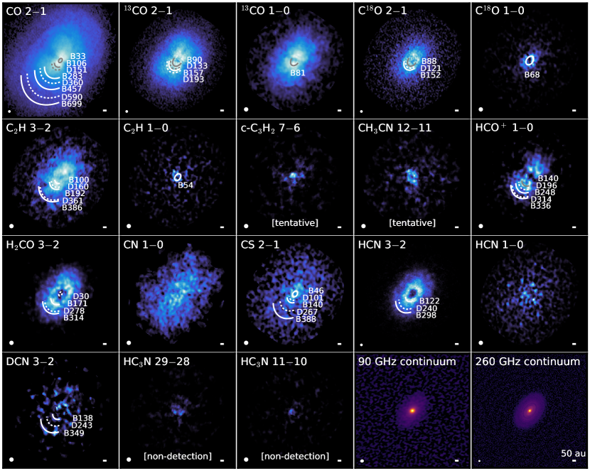
Figure 27.1: Zeroth moment maps for all lines targeted in this study and the 90 GHz and 260 GHz continuum in IM Lup. All panels show the same spatial scale. Otherwise, as in Figure 3.

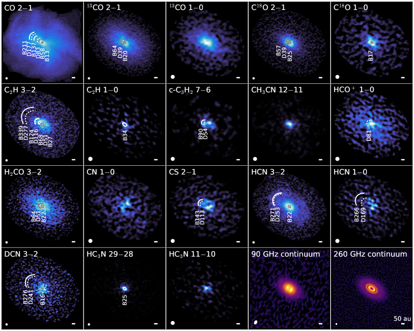
Figure 27.2: Zeroth moment maps for all lines targeted in this study and the 90 GHz and 260 GHz continuum in GM Aur. Otherwise, as in Figure 3.

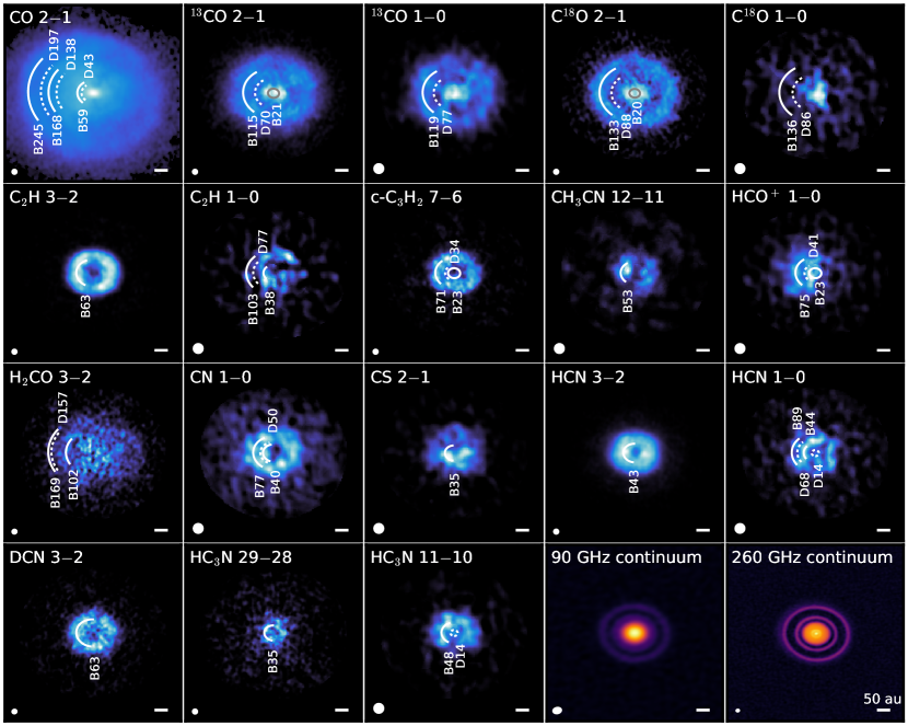
Figure 27.3: Zeroth moment maps for all lines targeted in this study and the 90 GHz and 260 GHz continuum in AS 209. Otherwise, as in Figure 3.

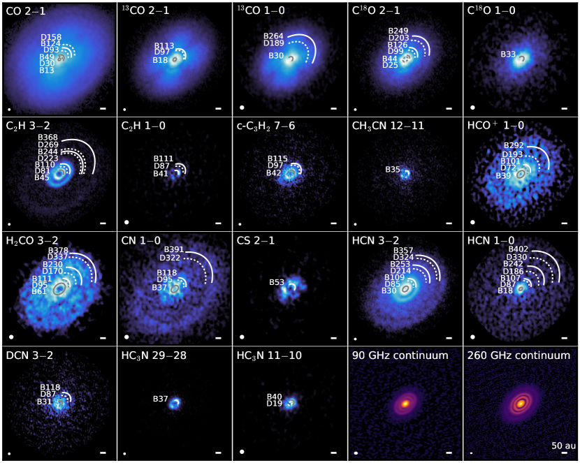
Figure 27.4: Zeroth moment maps for all lines targeted in this study and the 90 GHz and 260 GHz continuum in HD 163296. Otherwise, as in Figure 3.

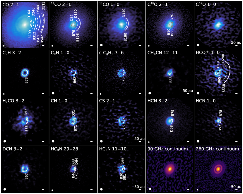
Figure 27.5: Zeroth moment maps for all lines targeted in this study and the 90 GHz and 260 GHz continuum in MWC 480. Otherwise, as in Figure 3.

Appendix C Peak intensity maps

Figure 28.1 shows peak intensity maps for the CO lines in all MAPS disks. A complete gallery of peak intensity maps for all 18 lines considered here is shown in Figure Set 2, which is available in the electronic edition of the journal.

Fig. Set 28. MAPS Peak Intensity Maps

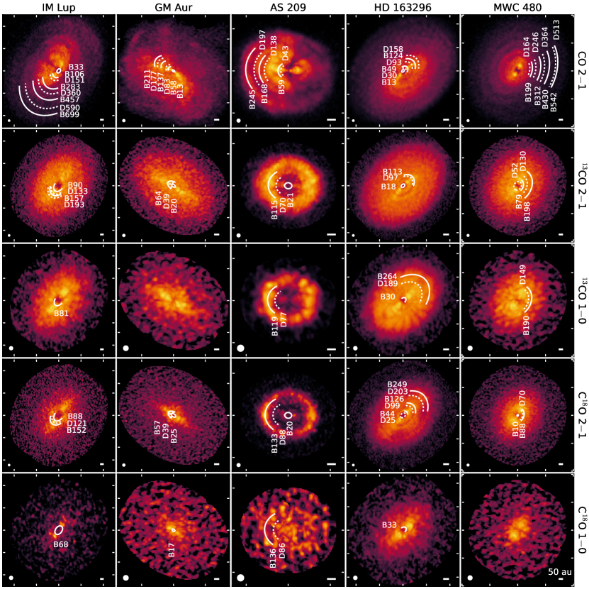
Figure 28.1: Peak intensity maps of CO, ¹³CO, and C¹⁸O lines. Otherwise, as in Figure 3.

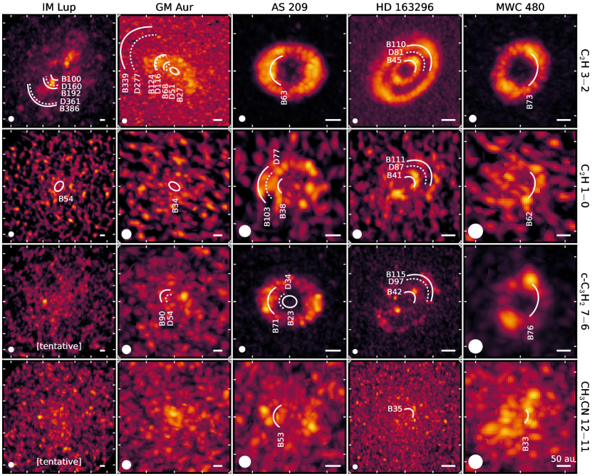
Figure 28.2: Peak intensity maps of C₂H, c-C₃H₂, and CH₃CN lines. Otherwise, as in Figure 3.

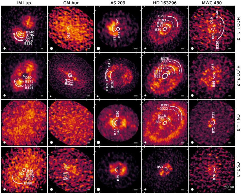
Figure 28.3: Peak intensity maps of HCO⁺, H₂CO, CN, and CS lines. Otherwise, as in Figure 3.

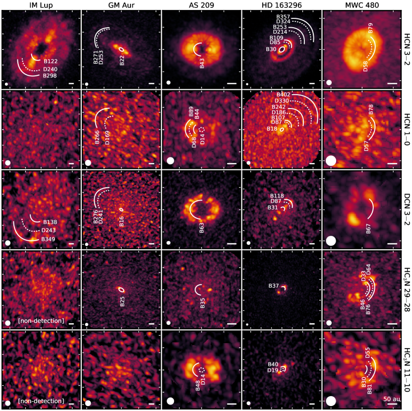
Figure 28.4: Peak intensity maps of HCN, DCN, and HC₃N lines. Otherwise, as in Figure 3.

Appendix D Surface Assumptions on Radial Profiles

Figure 29 shows the effects of considering emission surfaces, when they could be constrained (Law et al., 2021), during the radial profile deprojection process. The CO 2–1 lines are shown for all MAPS disks, as they possess the most elevated emitting surfaces. In all cases, the shape of radial intensity profile is not altered but the inclusion of an emitting surface often leads to the emergence of additional low-contrast features or sharpens the contrasts of existing substructures.

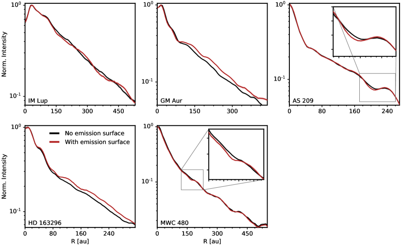
Figure 29: Normalized radial intensity profiles for CO 2–1 that are deprojected with (red) and without (black) the emission surfaces derived in Law et al. (2021).

Appendix E Logarithmically-scaled CO radial intensity profiles

To better illustrate low-contrast substructures and those at large radii present in the CO isotopologues, Figure 30 shows logarithmically-scaled radial intensity profiles.

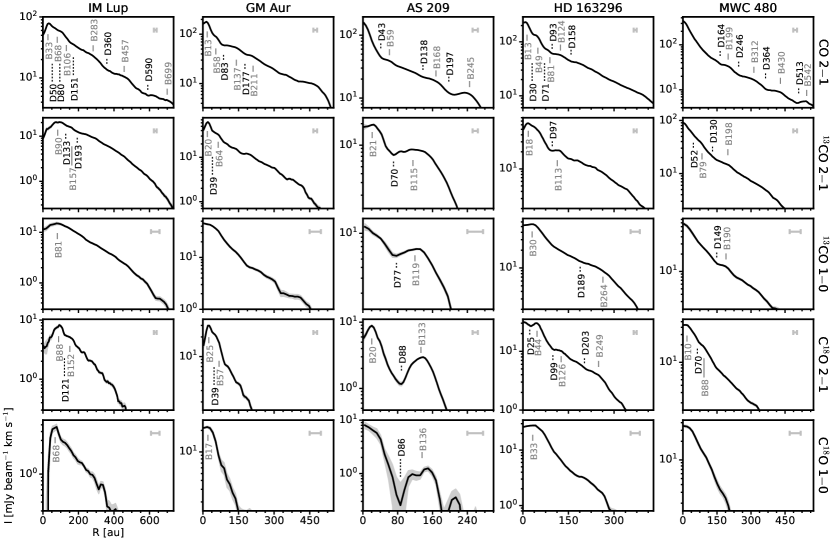
Figure 30: Deprojected radial intensity profiles of CO lines, as in Figure 9, but logarithmically-scaled to highlight low-contrast substructures.

Appendix F Full Tables of Fitted Substructure Characteristics

For readability, Tables 3–5 are listed in this Appendix.

F.1 Detected features

A full list of radial chemical substructures is found in Table 3.

Table 3: Properties of Radial Chemical Substructures

Source	Line	Feature	r0	r0	Method	Width	Depth
			[mas]	[au]		[au]
(1)	(2)	(3)	(4)	(5)	(6)	(7)	(8)
IM Lup	CO 2$-$1	B33‡	210.7 $\pm$ 1.0	33.3 $\pm$ 0.2	G	67 $\pm$ 2	$-$
		D50	${\sim}$316	${\sim}$50	V	$-$	$-$
		B68	${\sim}$430	${\sim}$68	V	$-$	$-$
		D80	${\sim}$506	${\sim}$80	V	$-$	$-$
		B106	673.8 $\pm$ 1.0	106.5 $\pm$ 0.2	G	93 $\pm$ 1	$-$
		D151	${\sim}$956	${\sim}$151	V	$-$	$-$
		B283	1788.6 $\pm$ 6.8	282.6 $\pm$ 1.1	G	134 $\pm$ 3	$-$
		D360	2278.2 $\pm$ 11.5	360.0 $\pm$ 1.8	G	55 $\pm$ 18	$-$
		B457	2893.5 $\pm$ 5.8	457.2 $\pm$ 0.9	G	49 $\pm$ 7	$-$
		D590	${\sim}$3734	${\sim}$590	V	$-$	$-$
		B699	4424.7 $\pm$ 0.8	699.1 $\pm$ 0.1	G	31 $\pm$ 2	$-$
	13CO 2$-$1	B90	568.7 $\pm$ 5.4	89.8 $\pm$ 0.9	G	164 $\pm$ 6	$-$
		D133	${\sim}$842	${\sim}$133	V	$-$	$-$
		B157	${\sim}$994	${\sim}$157	V	$-$	$-$
		D193	${\sim}$1222	${\sim}$193	V	$-$	$-$
	13CO 1$-$0	B81‡	514.8 $\pm$ 34.1	81.3 $\pm$ 5.4	G	240 $\pm$ 5	$-$
	C18O 2$-$1	B88	559.1 $\pm$ 2.6	88.3 $\pm$ 0.4	G	51 $\pm$ 3	$-$
		D121	${\sim}$766	${\sim}$121	V	$-$	$-$
		B152	959.5 $\pm$ 10.6	151.6 $\pm$ 1.7	G	96 $\pm$ 8	$-$
	C18O 1$-$0	B68	433.4 $\pm$ 8.1	68.5 $\pm$ 1.3	G	80 $\pm$ 5	$-$
	C2H 3$-$2	B100	634.1 $\pm$ 11.4	100.2 $\pm$ 1.8	G	87 $\pm$ 4	$-$
		D160	${\sim}$1013	${\sim}$160	V	$-$	$-$
		B192	1214.1 $\pm$ 17.5	191.8 $\pm$ 2.8	G	103 $\pm$ 8	$-$
		D361†	2287.5 $\pm$ 75.0	361.4 $\pm$ 11.8	R	12 $\pm$ 2	0.96 $\pm$ 0.07
		B386	2441.6 $\pm$ 4.7	385.8 $\pm$ 0.7	G	141 $\pm$ 8	$-$
	C2H 1$-$0	B54	343.3 $\pm$ 26.8	54.2 $\pm$ 4.2	G	55 $\pm$ 16	$-$
	H2CO 3$-$2	D30‡	187.5 $\pm$ 75.0	29.6 $\pm$ 11.8	R	$>$59	0.37 $\pm$ 0.12
		B171	1082.0 $\pm$ 40.7	171.0 $\pm$ 6.4	G	281 $\pm$ 13	$-$
		D278	${\sim}$1759	${\sim}$278	V	$-$	$-$
		B314	${\sim}$1987	${\sim}$314	V	$-$	$-$
	HCO+ 1$-$0	B140	888.2 $\pm$ 6.9	140.3 $\pm$ 1.1	G	120 $\pm$ 6	$-$
		D196†	1237.5 $\pm$ 75.0	195.5 $\pm$ 11.8	R	8 $\pm$ 8	0.96 $\pm$ 0.06
		B248	1570.7 $\pm$ 7.1	248.2 $\pm$ 1.1	G	76 $\pm$ 1	$-$
		D314†	1987.5 $\pm$ 75.0	314.0 $\pm$ 11.8	R	17 $\pm$ 2	0.92 $\pm$ 0.07
		B336	2124.5 $\pm$ 4.1	335.7 $\pm$ 0.7	G	80 $\pm$ 1	$-$
	CS 2$-$1	B46	288.6 $\pm$ 2.7	45.6 $\pm$ 0.4	G	58 $\pm$ 0.2	$-$
		D101†	637.5 $\pm$ 75.0	100.7 $\pm$ 11.8	R	46 $\pm$ 3	0.86 $\pm$ 0.11
		B140	887.8 $\pm$ 5.8	140.3 $\pm$ 0.9	G	93 $\pm$ 4	$-$
		D267†	1687.5 $\pm$ 75.0	266.6 $\pm$ 11.8	R	39 $\pm$ 2	0.54 $\pm$ 0.12
		B388	2454.2 $\pm$ 24.1	387.8 $\pm$ 3.8	G	292 $\pm$ 15	$-$
	HCN 3$-$2	B122	769.0 $\pm$ 3.4	121.5 $\pm$ 0.5	G	126 $\pm$ 2	$-$
		D240	${\sim}$1519	${\sim}$240	V	$-$	$-$
		B298	1885.2 $\pm$ 5.7	297.9 $\pm$ 0.9	G	177 $\pm$ 2	$-$
	DCN 3$-$2	B138	873.5 $\pm$ 84.8	138.0 $\pm$ 13.4	G	92 $\pm$ 40	$-$
		D243	1537.5 $\pm$ 75.0	242.9 $\pm$ 11.8	R	130 $\pm$ 2	0.12 $\pm$ 0.15
		B349	2205.9 $\pm$ 9.2	348.5 $\pm$ 1.4	G	98 $\pm$ 15	$-$
GM Aur	CO 2$-$1	B13‡	80.1 $\pm$ 2.3	12.7 $\pm$ 0.4	G	56 $\pm$ 1	$-$
		B58†	366.9 $\pm$ 1.5	58.3 $\pm$ 0.2	G	14 $\pm$ 2	$-$
		D83	521.7 $\pm$ 3.8	83.0 $\pm$ 0.6	G	28 $\pm$ 6	$-$
		B137	860.5 $\pm$ 10.4	136.8 $\pm$ 1.7	G	31 $\pm$ 3	$-$
		D177b	1113.8 $\pm$ 2.2	177.1 $\pm$ 0.4	G	24 $\pm$ 3	$-$
		B211${}^{{\dagger}}{}^{b}$	1329.7 $\pm$ 3.0	211.4 $\pm$ 0.5	G	20 $\pm$ 7	$-$
	13CO 2$-$1	B20‡	128.5 $\pm$ 2.6	20.4 $\pm$ 0.4	G	41 $\pm$ 3	$-$
		D39	${\sim}$245	${\sim}$39	V	$-$	$-$
		B64	403.8 $\pm$ 1.5	64.2 $\pm$ 0.2	G	34 $\pm$ 3	$-$
	C18O 2$-$1	B25	155.9 $\pm$ 0.6	24.8 $\pm$ 0.1	G	38 $\pm$ 3	$-$
		D39	${\sim}$245	${\sim}$39	V	$-$	$-$
		B57	${\sim}$358	${\sim}$57	V	$-$	$-$
	C18O 1$-$0	B17‡	106.7 $\pm$ 11.9	17.0 $\pm$ 1.9	G	98 $\pm$ 1	$-$
	C2H 3$-$2	B27	168.3 $\pm$ 1.9	26.8 $\pm$ 0.3	G	47 $\pm$ 1	$-$
		D51†	318.7 $\pm$ 37.5	50.7 $\pm$ 6.0	R	12 $\pm$ 0.2	0.82 $\pm$ 0.07
		B68	428.5 $\pm$ 0.4	68.1 $\pm$ 0.1	G	48 $\pm$ 2	$-$
		D116†	731.2 $\pm$ 37.5	116.3 $\pm$ 6.0	R	7 $\pm$ 4	0.93 $\pm$ 0.09
		B124	779.7 $\pm$ 1.8	124.0 $\pm$ 0.3	G	47 $\pm$ 4	$-$
		D277	${\sim}$1742	${\sim}$277	V	67 $\pm$ 1	$-$
		B339	2133.6 $\pm$ 3.2	339.2 $\pm$ 0.5	G	53 $\pm$ 8	$-$
	C2H 1$-$0	B34†	216.6 $\pm$ 10.9	34.4 $\pm$ 1.7	G	47 $\pm$ 12	$-$
	c-C3H2 7$-$6	D54	337.5 $\pm$ 75.0	53.7 $\pm$ 11.9	R	$>$55	0.58 $\pm$ 0.21
		B90	567.6 $\pm$ 7.3	90.3 $\pm$ 1.2	G	85 $\pm$ 5	$-$
	H2CO 3$-$2	B22	140.3 $\pm$ 2.1	22.3 $\pm$ 0.3	G	40 $\pm$ 7	$-$
		D51†	318.7 $\pm$ 37.5	50.7 $\pm$ 6.0	R	14 $\pm$ 0.5	0.86 $\pm$ 0.08
		B64	402.4 $\pm$ 3.0	64.0 $\pm$ 0.5	G	40 $\pm$ 5	$-$
	HCO+ 1$-$0	D81†	511.9 $\pm$ 78.8	81.4 $\pm$ 12.5	R	${\sim}$30	$-$
	CS 2$-$1	D113†	711.7 $\pm$ 74.9	113.2 $\pm$ 11.9	R	15 $\pm$ 14	$-$
		B143	899.6 $\pm$ 102.3	143.0 $\pm$ 16.3	G	129 $\pm$ 28	$-$
	HCN 3$-$2	B22‡	136.2 $\pm$ 1.7	21.7 $\pm$ 0.3	G	52 $\pm$ 1	$-$
		D253†	1593.7 $\pm$ 37.5	253.4 $\pm$ 6.0	R	20 $\pm$ 1	$-$
		B271	1705.2 $\pm$ 3.6	271.1 $\pm$ 0.6	G	95 $\pm$ 2	$-$
	HCN 1$-$0	D169†	1063.1 $\pm$ 78.7	169.0 $\pm$ 12.5	R	43 $\pm$ 5	$-$
		B266	1672.5 $\pm$ 46.3	265.9 $\pm$ 7.4	G	109 $\pm$ 54	$-$
	DCN 3$-$2	B16‡	100.6 $\pm$ 2.1	16.0 $\pm$ 0.3	G	35 $\pm$ 3	$-$
		D241	1518.7 $\pm$ 37.5	241.5 $\pm$ 6.0	R	$-$	$-$
		B276	1736.7 $\pm$ 13.6	276.1 $\pm$ 2.2	G	28 $\pm$ 16	$-$
	HC3N 29$-$28	B25	155.8 $\pm$ 0.6	24.8 $\pm$ 0.1	G	39 $\pm$ 1	$-$
AS 209	CO 2$-$1	D43	${\sim}$355	${\sim}$43	V	$-$	$-$
		B59†	486.2 $\pm$ 1.3	58.8 $\pm$ 0.2	G	17 $\pm$ 3	$-$
		D138	${\sim}$1140	${\sim}$138	V	$-$	$-$
		B168	1385.9 $\pm$ 7.8	167.7 $\pm$ 0.9	G	23 $\pm$ 4	$-$
		D197	1631.4 $\pm$ 0.4	197.4 $\pm$ 0.04	G	21 $\pm$ 2	$-$
		B245	2026.3 $\pm$ 1.4	245.2 $\pm$ 0.2	G	44 $\pm$ 1	$-$
	13CO 2$-$1	B21‡	174.7 $\pm$ 2.7	21.1 $\pm$ 0.3	G	48 $\pm$ 0.3	$-$
		D70	581.2 $\pm$ 37.5	70.3 $\pm$ 4.5	R	19 $\pm$ 1	0.84 $\pm$ 0.02
		B115	950.3 $\pm$ 1.0	115.0 $\pm$ 0.1	G	142 $\pm$ 1	$-$
	13CO 1$-$0	D77†	637.5 $\pm$ 75.0	77.1 $\pm$ 9.1	R	32 $\pm$ 2	0.83 $\pm$ 0.04
		B119	987.2 $\pm$ 3.4	119.5 $\pm$ 0.4	G	103 $\pm$ 2	$-$
	C18O 2$-$1	B20	167.4 $\pm$ 2.2	20.2 $\pm$ 0.3	G	40 $\pm$ 3	$-$
		D88	731.2 $\pm$ 37.5	88.5 $\pm$ 4.5	R	47 $\pm$ 0.1	0.40 $\pm$ 0.03
		B133	1102.8 $\pm$ 1.0	133.4 $\pm$ 0.1	G	66 $\pm$ 1	$-$
	C18O 1$-$0	D86†	712.5 $\pm$ 75.0	86.2 $\pm$ 9.1	R	27 $\pm$ 8	0.28 $\pm$ 0.45
		B136	1122.4 $\pm$ 30.8	135.8 $\pm$ 3.7	G	72 $\pm$ 12	$-$
	C2H 3$-$2	B63	522.7 $\pm$ 1.7	63.2 $\pm$ 0.2	G	70 $\pm$ 1	$-$
	C2H 1$-$0	B38	314.8 $\pm$ 10.4	38.1 $\pm$ 1.3	G	55 $\pm$ 9	$-$
		D77†	637.5 $\pm$ 75.0	77.1 $\pm$ 9.1	R	22 $\pm$ 1	0.48 $\pm$ 0.30
		B103†	853.9 $\pm$ 4.4	103.3 $\pm$ 0.5	G	30 $\pm$ 2	$-$
	c-C3H2 7$-$6	B23	193.9 $\pm$ 7.7	23.5 $\pm$ 0.9	G	34 $\pm$ 6	$-$
		D34†	281.2 $\pm$ 37.5	34.0 $\pm$ 4.5	R	9 $\pm$ 0.3	0.87 $\pm$ 0.15
		B71	583.4 $\pm$ 2.1	70.6 $\pm$ 0.3	G	57 $\pm$ 2	$-$
	H2CO 3$-$2	B102	839.8 $\pm$ 1.0	101.6 $\pm$ 0.1	G	63 $\pm$ 2	$-$
		D157†	1293.6 $\pm$ 37.5	156.5 $\pm$ 4.5	R	13 $\pm$ 1	0.92 $\pm$ 0.06
		B169	1396.4 $\pm$ 8.0	169.0 $\pm$ 1.0	G	51 $\pm$ 1	$-$
	HCO+ 1$-$0	B23	188.3 $\pm$ 16.8	22.8 $\pm$ 2.0	G	42 $\pm$ 1	$-$
		D41†	337.2 $\pm$ 74.9	40.8 $\pm$ 9.1	R	25 $\pm$ 2	0.58 $\pm$ 0.07
		B75	623.8 $\pm$ 6.3	75.5 $\pm$ 0.8	G	78 $\pm$ 1	$-$
	CS 2$-$1	B35‡	291.5 $\pm$ 5.7	35.3 $\pm$ 0.7	G	82 $\pm$ 0.3	$-$
	CN 1$-$0	B40	328.6 $\pm$ 19.7	39.8 $\pm$ 2.4	G	53 $\pm$ 3	$-$
		D50†	412.5 $\pm$ 75.0	49.9 $\pm$ 9.1	R	14 $\pm$ 8	0.91 $\pm$ 0.15
		B77	636.1 $\pm$ 2.2	77.0 $\pm$ 0.3	G	50 $\pm$ 1	$-$
	HCN 3$-$2	B43‡	359.1 $\pm$ 9.0	43.4 $\pm$ 1.1	G	96 $\pm$ 2	$-$
	HCN 1$-$0	D14	112.5 $\pm$ 75.0	13.6 $\pm$ 9.1	R	$>$27	0.39 $\pm$ 0.08
		B44	363.1 $\pm$ 4.1	43.9 $\pm$ 0.5	G	37 $\pm$ 1	$-$
		D68	${\sim}$562	${\sim}$68	V	$-$	$-$
		B89	739.2 $\pm$ 1.6	89.4 $\pm$ 0.2	G	64 $\pm$ 1	$-$
	DCN 3$-$2	B63	521.7 $\pm$ 6.1	63.1 $\pm$ 0.7	G	74 $\pm$ 3	$-$
	HC3N 29$-$28	B35	287.1 $\pm$ 0.4	34.7 $\pm$ 0.05	G	27 $\pm$ 3	$-$
	HC3N 11$-$10	D14‡	112.5 $\pm$ 75.0	13.6 $\pm$ 9.1	R	$>$29	0.67 $\pm$ 0.11
		B48‡	397.5 $\pm$ 21.6	48.1 $\pm$ 2.6	G	99 $\pm$ 5	$-$
	CH3CN 12$-$11	B53	436.2 $\pm$ 102.1	52.8 $\pm$ 12.4	G	72 $\pm$ 25	$-$
HD 163296	CO 2$-$1	B13†	124.7 $\pm$ 3.7	12.6 $\pm$ 0.4	G	9 $\pm$ 3	$-$
		D30†	299.4 $\pm$ 4.6	30.2 $\pm$ 0.5	G	13 $\pm$ 2	$-$
		B49	489.8 $\pm$ 1.9	49.5 $\pm$ 0.2	G	16 $\pm$ 1	$-$
		D71†	704.8 $\pm$ 1.9	71.2 $\pm$ 0.2	G	14 $\pm$ 2	$-$
		B81	${\sim}$802	${\sim}$81	V	$-$	$-$
		D93	924.7 $\pm$ 6.2	93.4 $\pm$ 0.6	G	17 $\pm$ 3	$-$
		B124	1222.9 $\pm$ 5.8	123.5 $\pm$ 0.6	G	25 $\pm$ 3	$-$
		D158	1568.1 $\pm$ 2.7	158.4 $\pm$ 0.3	G	24 $\pm$ 3	$-$
	13CO 2$-$1	B18‡	176.1 $\pm$ 5.6	17.8 $\pm$ 0.6	G	54 $\pm$ 2	$-$
		D97†	956.2 $\pm$ 37.5	96.6 $\pm$ 3.8	R	9 $\pm$ 1	0.98 $\pm$ 0.02
		B113	1120.3 $\pm$ 2.2	113.2 $\pm$ 0.2	G	85 $\pm$ 1	$-$
	13CO 1$-$0	B30‡	299.9 $\pm$ 6.6	30.3 $\pm$ 0.7	G	89 $\pm$ 1	$-$
		D189	1868.3 $\pm$ 6.4	188.7 $\pm$ 0.6	G	49 $\pm$ 14	$-$
		B264	2609.2 $\pm$ 31.0	263.5 $\pm$ 3.1	G	67 $\pm$ 10	$-$
	C18O 2$-$1	D25	243.7 $\pm$ 37.5	24.6 $\pm$ 3.8	R	19 $\pm$ 1	0.89 $\pm$ 0.03
		B44	431.1 $\pm$ 2.1	43.5 $\pm$ 0.2	G	61 $\pm$ 3	$-$
		D99†	980.1 $\pm$ 3.8	99.0 $\pm$ 0.4	G	13 $\pm$ 3	$-$
		B126	1248.5 $\pm$ 4.7	126.1 $\pm$ 0.5	G	20 $\pm$ 6	$-$
		D203	2006.3 $\pm$ 22.1	202.6 $\pm$ 2.2	G	28 $\pm$ 7	$-$
		B249	2468.4 $\pm$ 2.4	249.3 $\pm$ 0.2	G	39 $\pm$ 2	$-$
	C18O 1$-$0	B33‡	322.9 $\pm$ 8.7	32.6 $\pm$ 0.9	G	102 $\pm$ 6	$-$
	C2H 3$-$2	B45	444.3 $\pm$ 1.0	44.9 $\pm$ 0.1	G	34 $\pm$ 1	$-$
		D81	806.2 $\pm$ 37.5	81.4 $\pm$ 3.8	R	27 $\pm$ 0.5	0.49 $\pm$ 0.01
		B110	1087.6 $\pm$ 2.4	109.8 $\pm$ 0.2	G	49 $\pm$ 0.1	$-$
		D223a	2212.5 $\pm$ 75.0	223.5 $\pm$ 7.6	R	28 $\pm$ 8	0.55 $\pm$ 0.15
		B244a	2418.6 $\pm$ 0.6	244.3 $\pm$ 0.1	G	37 $\pm$ 2	$-$
		D269a	2662.5 $\pm$ 75.0	268.9 $\pm$ 7.6	R	71 $\pm$ 56	0.23 $\pm$ 0.06
		B368a	3638.7 $\pm$ 4.1	367.5 $\pm$ 0.4	G	116 $\pm$ 3	$-$
	C2H 1$-$0	B41	407.4 $\pm$ 2.0	41.1 $\pm$ 0.2	G	40 $\pm$ 1	$-$
		D87†	862.5 $\pm$ 75.0	87.1 $\pm$ 7.6	R	18 $\pm$ 1	0.08 $\pm$ 0.15
		B111	1094.7 $\pm$ 8.3	110.6 $\pm$ 0.8	G	35 $\pm$ 2	$-$
	c-C3H2 7$-$6	B42	414.4 $\pm$ 21.5	41.9 $\pm$ 2.2	G	44 $\pm$ 6	$-$
		D97	956.2 $\pm$ 37.5	96.6 $\pm$ 3.8	R	${\sim}$30	$-$
		B115	1142.0 $\pm$ 0.9	115.3 $\pm$ 0.1	G	29 $\pm$ 1	$-$
	H2CO 3$-$2	B61	603.3 $\pm$ 15.7	60.9 $\pm$ 1.6	G	46 $\pm$ 5	$-$
		D95	${\sim}$941	${\sim}$95	V	$-$	$-$
		B111	1095.8 $\pm$ 14.2	110.7 $\pm$ 1.4	G	85 $\pm$ 3	$-$
		D170	1687.5 $\pm$ 75.0	170.4 $\pm$ 7.6	R	47 $\pm$ 0.2	0.78 $\pm$ 0.07
		B230	2275.3 $\pm$ 11.4	229.8 $\pm$ 1.2	G	157 $\pm$ 1	$-$
		D337	${\sim}$3337	${\sim}$337	V	$-$	$-$
		B378	3746.9 $\pm$ 4.0	378.4 $\pm$ 0.4	G	114 $\pm$ 3	$-$
	HCO+ 1$-$0	B39	386.6 $\pm$ 0.9	39.1 $\pm$ 0.1	G	50 $\pm$ 4	$-$
		D72	${\sim}$713	${\sim}$72	V	$-$	$-$
		B101	996.7 $\pm$ 6.3	100.7 $\pm$ 0.6	G	115 $\pm$ 1	$-$
		D193	1912.5 $\pm$ 75.0	193.2 $\pm$ 7.6	R	63 $\pm$ 1	0.77 $\pm$ 0.10
		B292	2892.3 $\pm$ 14.8	292.1 $\pm$ 1.5	G	178 $\pm$ 9	$-$
	CS 2$-$1	B53‡	528.2 $\pm$ 25.5	53.3 $\pm$ 2.6	G	129 $\pm$ 4	$-$
	CN 1$-$0	B37	371.0 $\pm$ 0.7	37.5 $\pm$ 0.1	G	57 $\pm$ 2	$-$
		D95†	937.5 $\pm$ 75.0	94.7 $\pm$ 7.6	R	20 $\pm$ 3	0.90 $\pm$ 0.06
		B118	1173.0 $\pm$ 6.1	118.5 $\pm$ 0.6	G	75 $\pm$ 0.3	$-$
		D322	3187.5 $\pm$ 75.0	321.9 $\pm$ 7.6	R	46 $\pm$ 0.4	0.62 $\pm$ 0.04
		B391	3871.6 $\pm$ 6.0	391.0 $\pm$ 0.6	G	168 $\pm$ 3	$-$
	HCN 3$-$2	B30	299.3 $\pm$ 3.8	30.2 $\pm$ 0.4	G	55 $\pm$ 1	$-$
		D85	843.8 $\pm$ 37.5	85.2 $\pm$ 3.8	R	22 $\pm$ 0.3	0.75 $\pm$ 0.02
		B109	1079.2 $\pm$ 0.0	109.0 $\pm$ 0.00	G	51 $\pm$ 1	$-$
		D214	2118.8 $\pm$ 37.5	214.0 $\pm$ 3.8	R	36 $\pm$ 0.2	0.95 $\pm$ 0.02
		B253	2506.2 $\pm$ 2.8	253.1 $\pm$ 0.3	G	108 $\pm$ 2	$-$
		D324	3206.2 $\pm$ 37.5	323.8 $\pm$ 3.8	R	26 $\pm$ 0.3	0.83 $\pm$ 0.03
		B357	3536.7 $\pm$ 3.4	357.2 $\pm$ 0.3	G	106 $\pm$ 1	$-$
	HCN 1$-$0	B18‡	173.9 $\pm$ 3.0	17.6 $\pm$ 0.3	G	54 $\pm$ 1	$-$
		D87†	862.5 $\pm$ 75.0	87.1 $\pm$ 7.6	R	19 $\pm$ 0.3	0.42 $\pm$ 0.15
		B107	1055.5 $\pm$ 1.7	106.6 $\pm$ 0.2	G	33 $\pm$ 4	$-$
		D186†	1837.5 $\pm$ 75.0	185.6 $\pm$ 7.6	R	22 $\pm$ 5	0.44 $\pm$ 0.15
		B242	2398.0 $\pm$ 41.4	242.2 $\pm$ 4.2	G	99 $\pm$ 21	$-$
		D330	3262.5 $\pm$ 75.0	329.5 $\pm$ 7.6	R	55 $\pm$ 2	0.30 $\pm$ 0.19
		B402	3983.2 $\pm$ 29.2	402.3 $\pm$ 2.9	G	124 $\pm$ 10	$-$
	DCN 3$-$2	B31‡	307.0 $\pm$ 90.4	31.0 $\pm$ 9.1	G	72 $\pm$ 14	$-$
		D87†	862.5 $\pm$ 75.0	87.1 $\pm$ 7.6	R	28 $\pm$ 0.2	0.59 $\pm$ 0.12
		B118	1168.3 $\pm$ 8.5	118.0 $\pm$ 0.9	G	45 $\pm$ 1	$-$
	HC3N 29$-$28	B37	362.5 $\pm$ 1.5	36.6 $\pm$ 0.1	G	43 $\pm$ 1	$-$
	HC3N 11$-$10	D19	187.5 $\pm$ 75.0	18.9 $\pm$ 7.6	R	$>$27	0.79 $\pm$ 0.26
		B40	397.1 $\pm$ 22.1	40.1 $\pm$ 2.2	G	52 $\pm$ 3	$-$
	CH3CN 12$-$11	B35	344.5 $\pm$ 1.2	34.8 $\pm$ 0.1	G	33 $\pm$ 0.3	$-$
MWC 480	CO 2$-$1	D164†	1013.8 $\pm$ 5.1	164.0 $\pm$ 0.8	G	20 $\pm$ 3	$-$
		B199	1231.3 $\pm$ 0.7	199.2 $\pm$ 0.1	G	28 $\pm$ 3	$-$
		D246	1517.7 $\pm$ 7.1	245.6 $\pm$ 1.1	G	43 $\pm$ 4	$-$
		B312	1931.2 $\pm$ 3.4	312.5 $\pm$ 0.6	G	45 $\pm$ 4	$-$
		D364†	2247.7 $\pm$ 2.6	363.7 $\pm$ 0.4	G	20 $\pm$ 2	$-$
		B430	2655.7 $\pm$ 1.6	429.7 $\pm$ 0.3	G	62 $\pm$ 3	$-$
		D513†	${\sim}$3171	${\sim}$513	V	20 $\pm$ 2	0.97 $\pm$ 0.01
		B542	3350.7 $\pm$ 1.8	542.1 $\pm$ 0.3	G	55 $\pm$ 3	$-$
	13CO 2$-$1	D52	${\sim}$321	${\sim}$52	V	$-$	$-$
		B79†	490.4 $\pm$ 5.5	79.3 $\pm$ 0.9	G	19 $\pm$ 8	$-$
		D130	806.0 $\pm$ 37.0	130.4 $\pm$ 6.0	G	66 $\pm$ 33	$-$
		B198	1223.9 $\pm$ 2.2	198.0 $\pm$ 0.4	G	37 $\pm$ 10	$-$
	13CO 1$-$0	D149†	921.0 $\pm$ 6.2	149.0 $\pm$ 1.0	G	25 $\pm$ 7	$-$
		B190†	1174.1 $\pm$ 6.3	190.0 $\pm$ 1.0	G	28 $\pm$ 13	$-$
	C18O 2$-$1	B10‡	61.8 $\pm$ 14.1	10.0 $\pm$ 2.3	G	104 $\pm$ 7	$-$
		D70	${\sim}$433	${\sim}$70	V	$-$	$-$
		B88	${\sim}$544	${\sim}$88	V	$-$	$-$
	C2H 3$-$2	B73	449.9 $\pm$ 3.4	72.8 $\pm$ 0.5	G	64 $\pm$ 2	$-$
	C2H 1$-$0	B62	385.7 $\pm$ 16.1	62.4 $\pm$ 2.6	G	54 $\pm$ 8	$-$
	c-C3H2 7$-$6	B76	472.0 $\pm$ 5.4	76.4 $\pm$ 0.9	G	65 $\pm$ 3	$-$
	H2CO 3$-$2	D55†	337.5 $\pm$ 75.0	54.6 $\pm$ 12.1	R	25 $\pm$ 3	0.75 $\pm$ 0.17
		B86	531.5 $\pm$ 10.0	86.0 $\pm$ 1.6	G	77 $\pm$ 16	$-$
	HCO+ 1$-$0	D19†	118.1 $\pm$ 78.7	19.1 $\pm$ 12.7	R	33 $\pm$ 0.2	0.17 $\pm$ 0.24
		B65	401.0 $\pm$ 4.8	64.9 $\pm$ 0.8	G	62 $\pm$ 4	$-$
		D248	1535.6 $\pm$ 78.7	248.5 $\pm$ 12.7	R	52 $\pm$ 2	0.13 $\pm$ 0.16
		B330	2039.4 $\pm$ 8.8	330.0 $\pm$ 1.4	G	143 $\pm$ 34	$-$
	CS 2$-$1	B76	468.1 $\pm$ 34.7	75.7 $\pm$ 5.6	G	82 $\pm$ 12	$-$
	CN 1$-$0	D31	190.6 $\pm$ 76.2	30.8 $\pm$ 12.3	R	$>$44	0.57 $\pm$ 0.17
		B71	436.1 $\pm$ 8.1	70.6 $\pm$ 1.3	G	76 $\pm$ 4	$-$
	HCN 3$-$2	D58	${\sim}$358	${\sim}$58	V	$-$	$-$
		B79	489.0 $\pm$ 5.2	79.1 $\pm$ 0.8	G	54 $\pm$ 1	$-$
	HCN 1$-$0	D57	${\sim}$352	${\sim}$57	V	$-$	$-$
		B78†	479.5 $\pm$ 20.8	77.6 $\pm$ 3.4	G	36 $\pm$ 2	$-$
	DCN 3$-$2	B67	417.1 $\pm$ 2.1	67.5 $\pm$ 0.3	G	75 $\pm$ 3	$-$
	HC3N 29$-$28	D33	${\sim}$204	${\sim}$33	V	$-$	$-$
		B46†	282.6 $\pm$ 10.0	45.7 $\pm$ 1.6	G	24 $\pm$ 4	$-$
		D64	${\sim}$396	${\sim}$64	V	$-$	$-$
		B76	470.0 $\pm$ 8.6	76.0 $\pm$ 1.4	G	44 $\pm$ 2	$-$
	HC3N 11$-$10	B30†	184.1 $\pm$ 31.2	29.8 $\pm$ 5.1	G	47 $\pm$ 4	$-$
		D55	${\sim}$340	${\sim}$55	V	$-$	$-$
		B81	503.4 $\pm$ 22.5	81.5 $\pm$ 3.6	G	56 $\pm$ 10	$-$
	CH3CN 12$-$11	B33‡	202.6 $\pm$ 16.2	32.8 $\pm$ 2.6	G	91 $\pm$ 2	$-$

Note. — Column descriptions: (1) Name of host star. (2) Name of line. (3) Substructure label: “B” (“bright”) prefix refers to rings and “D” (“dark”) refers to gaps. (4) Radial location of substructure in mas (the uncertainties in mas are simply scaled from the fitting procedure and do not account for the uncertainty in the distance to the source). (5) Radial location of substructure in au. (6) Method used to derive radial location of substructure: “G” indicates Gaussian-fitting, “R” indicates identification of local extrema in the radial profiles, and “V” indicates identification through visual inspection. (7) Width of substructure. (8) Depth of gap, defined as the intensity ratio of adjacent ring-gap pairs (see Section 3.2). All uncertainties are 1$\sigma$.

F.2 Tentative features

A list of tentative radial chemical substructures is found in Table 4.

Table 4: List of Tentative and Asymmetric Radial Substructures

Source	Line	Feature	Nearest ID	r0	r0	Comments
				[mas]	[au]
(1)	(2)	(3)	(4)	(5)	(6)	(7)
IM Lup	HCN 1$-$0	Plateau	$\ldots$	1.27–3.32	200–525
GM Aur	HCO+ 1–0	Plateau	$\ldots$	0.63–2.70	100–430
	H2CO 3–2	Plateau	$\ldots$	0.94–2.70	150–430
	CN 1$-$0	Shoulder	$\ldots$	70	0.44	coincident with B64, H2CO 3–2
		Shoulder	$\ldots$	170	1.68	coincident with B143, CS 2–1
		Plateau	$\ldots$	1.38–2.83	220–450
AS 209	HCO+ 1–0	Shoulder	$\ldots$	0.99	120
	HCN 3$-$2	Radial asymmetry	B43	0.36	43	outward-sloping tail
	HC3N 29–28	Shoulder	$\ldots$	0.74	90	coincident with B89, HCN 1–0
	HC3N 11–10	Radial asymmetry	B48	0.40	48	outward-sloping tail
HD 163296	C2H 3–2	Shoulder	$\ldots$	0.10	10
	CS 2$-1$	Radial asymmetry	B53	0.52	53	outward-sloping tail
	HC3N 11–10	Shoulder	$\ldots$	0.99	100	coincident with B109, HCN 3–2; B107, HCN 1–0
MWC 480	C2H 3–2	Shoulder	$\ldots$	0.06	10
	CN 1–0	Plateau	$\ldots$	1.55–3.40	250–550
	DCN 3–2	Radial asymmetry	B67	0.41	67	outward-sloping tail

Note. — Column descriptions: (1) Name of host star. (2) Name of line. (3) Tentative substructure. “Shoulder” refers to localized emission plateau, while “plateau” refer to emission over a large radial extent. “Radial asymmetry” indicates an asymmetrical feature, as identified in the radial profiles. (4) Name of nearest identified substructure. (5) Radial location of substructure in mas. (6) Radial location of substructure in au. Radial locations are visually determined and approximate in nature. Formal uncertainties are not listed. (7) Comments about the tentative substructure.

F.3 Continuum substructures

A list of annular continuum substructures is found in Table 5.

Table 5: Properties of Annular Continuum Substructures

Source	Feature	r0	r0	Method	Width	Depth	Ref
		[mas]	[au]		[au]
(1)	(2)	(3)	(4)	(5)	(6)	(7)	(8)
IM Lup	D116	735 $\pm$ 23	116.18 $\pm$ 3.57	R	13.1 $\pm$ 0.2	0.83 $\pm$ 0.01	D117 (1)
	B133	844 $\pm$ 0.2	133.28 $\pm$ 0.03	G	50.2 $\pm$ 0.3	$-$	B134 (1)
	D209	${\sim}$1323	${\sim}$209	V	$-$	$-$
	B220	${\sim}$1392	${\sim}$220	V	$-$	$-$
	Redge	${\sim}$2025	${\sim}$320	V	$-$	$-$
GM Aur	D15	94	15.00	$-$	20.0	$-$	D15 (2)
	B42	264 $\pm$ 1	41.93 $\pm$ 0.18	G	31.8 $\pm$ 0.3	$-$	B40 (2)
	D68	425 $\pm$ 29	67.56 $\pm$ 4.66	R	13.5 $\pm$ 0.2	0.73 $\pm$ 0.05	D67 (2)
	B86	539 $\pm$ 1	85.66 $\pm$ 0.22	G	31.1 $\pm$ 1.0	$-$	B84 (2)
	D142	894 $\pm$ 29	142.10 $\pm$ 4.66	R	16.9 $\pm$ 0.5	0.96 $\pm$ 0.01	D145 (2)
	B163	1022 $\pm$ 2	162.51 $\pm$ 0.27	G	69.0 $\pm$ 0.4	$-$	B168 (2)
	Redge	${\sim}$1761	${\sim}$280	V	$-$	$-$
AS 209	D9	72	8.69	$-$	4.7	$-$	D9 (1)
	B14	117	14.20	$-$	8.9	$-$	B14 (1)
	D24	197	23.84	$-$	3.4	$-$	D24 (1)
	B28	230	27.80	$-$	4.7	$-$	B28 (1)
	D35	290	35.04	$-$	3.0	$-$	D35 (1)
	B39	320	38.70	$-$	3.4	$-$	B39 (1)
	D61	508 $\pm$ 25	61.43 $\pm$ 3.00	R	11.1 $\pm$ 0.8	0.38 $\pm$ 0.03	D61 (1)
	B74	611 $\pm$ 2	73.98 $\pm$ 0.20	G	17.2 $\pm$ 1.1	$-$	B74 (1)
	D100a	826 $\pm$ 0.0	100.00 $\pm$ 0.00	R	30.2 $\pm$ 0.7	0.06 $\pm$ 0.01	D90, B97, D105 (1)
	B121	1001 $\pm$ 0.2	121.18 $\pm$ 0.02	G	18.5 $\pm$ 0.8	$-$	B120 (1)
	D137	1132	137.00	$-$	4.2	$-$
	B141	1165	141.00	$-$	2.8	$-$
	Redge	${\sim}$1364	${\sim}$165	V	$-$	$-$
HD 163296	D10	99	10.00	$-$	3.2	$-$	D10 (1)
	B14	139	14.00	$-$	3.6	$-$	B14 (1)
	D49	490 $\pm$ 30	49.46 $\pm$ 3.00	R	17.3 $\pm$ 0.5	0.23 $\pm$ 0.03	D48 (1)
	B67	668 $\pm$ 0.4	67.44 $\pm$ 0.04	G	21.4 $\pm$ 0.7	$-$	B67 (1)
	D85	846 $\pm$ 30	85.44 $\pm$ 3.00	R	13.3 $\pm$ 0.5	0.40 $\pm$ 0.02	D86 (1)
	B101	998 $\pm$ 1	100.78 $\pm$ 0.09	G	20.5 $\pm$ 0.4	$-$	B100 (1)
	D145	1440 $\pm$ 30	145.39 $\pm$ 3.00	R	13.0 $\pm$ 0.1	0.85 $\pm$ 0.02	D145 (1)
	B159	1571 $\pm$ 0.3	158.70 $\pm$ 0.03	G	46.5 $\pm$ 0.4	$-$	B155 (1)
	Redge	${\sim}$2376	${\sim}$240	V	$-$	$-$
MWC 480	D76	467 $\pm$ 30	75.57 $\pm$ 4.88	R	24.8 $\pm$ 0.4	0.20 $\pm$ 0.01	D73 (3)
	B98	606 $\pm$ 0.1	98.10 $\pm$ 0.01	G	23.7 $\pm$ 0.3	$-$	B98 (3)
	D149	919 $\pm$ 30	148.71 $\pm$ 4.88	R	17.1 $\pm$ 0.1	0.82 $\pm$ 0.04
	B165	1023 $\pm$ 1	165.48 $\pm$ 0.08	G	51.6 $\pm$ 0.9	$-$
	Redge	${\sim}$1422	${\sim}$230	V	$-$	$-$

Note. — Column descriptions: (1) Name of host star. (2) Substructure label. (3) Radial location of substructure in mas (the uncertainties in mas are simply scaled from the fitting procedure and do not account for the uncertainty in the distance to the source). (4) Radial location of substructure in au. (5) Method used to derive radial location of substructure: “G” indicates Gaussian-fitting, “R” indicates identification of local extrema in radial profiles, and “V” indicates identification through visual inspection. (6) Width of substructure. (7) Depth of gap, defined as the intensity ratio of adjacent ring-gap pairs (see Section 3.2). All uncertainties are 1$\sigma$. (8) Reference for previously known annular continuum substructures. Italics indicate continuum substructures unresolved in MAPS that were from adopted from previous observations at higher spatial resolution. References: (1) Huang et al. (2018b); (2) Huang et al. (2020); (3) Long et al. (2018a).

Appendix G Relationship between chemical and NIR substructures

Figure 31 shows the radial locations of chemical substructures versus NIR rings in the three MAPS disks with known NIR substructure.

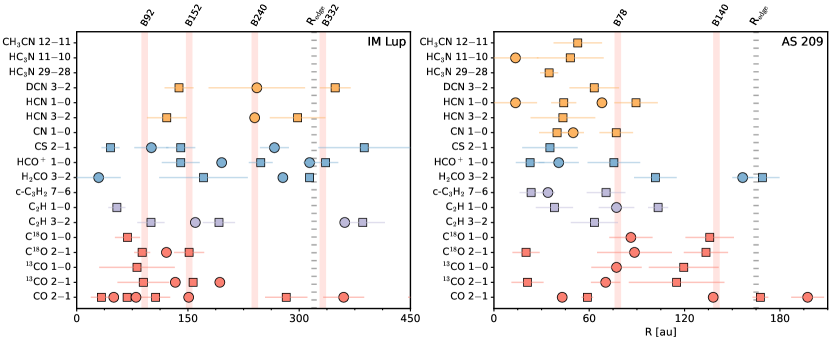
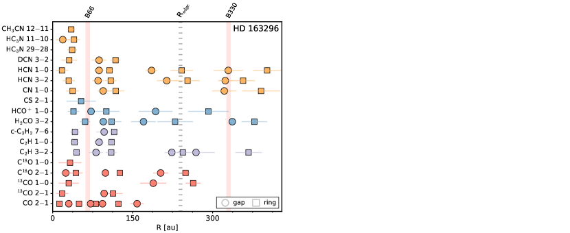
Figure 31: Radial locations of chemical substructures and NIR rings in IM Lup, AS 209, and HD 163296. Line emission rings and gaps are shown as squares and circles, respectively. Species are color-coded, as in Figures 15, 16, and 17. Red lines mark the radial locations of NIR rings (Monnier et al., 2017; Avenhaus et al., 2018). Broad dotted lines mark the location of the edge of millimeter continuum disk. Chemical substructures at large radii beyond the outermost NIR rings, which are only seen in CO 2–1, are omitted. The widths of error bars for chemical substructures represent $\sigma$ instead of the full FWHM, i.e., FWHM / 2.355, for visual clarity.

References

- Aikawa et al. (2021) Aikawa, Y., Cataldi, G., Yamato, Y., et al. 2021, arXiv e-prints, arXiv:2109.06419. https://arxiv.org/abs/2109.06419
- Akimkin et al. (2013) Akimkin, V., Zhukovska, S., Wiebe, D., et al. 2013, ApJ, 766, 8, doi: 10.1088/0004-637X/766/1/8
- Alarcón et al. (2020) Alarcón, F., Teague, R., Zhang, K., Bergin, E. A., & Barraza-Alfaro, M. 2020, ApJ, 905, 68, doi: 10.3847/1538-4357/abc1d6
- Alarcón et al. (2021) Alarcón, F., Bosman, A., Bergin, E., et al. 2021, arXiv e-prints, arXiv:2109.06263. https://arxiv.org/abs/2109.06263
- Alcalá et al. (2017) Alcalá, J. M., Manara, C. F., Natta, A., et al. 2017, A&A, 600, A20, doi: 10.1051/0004-6361/201629929
- ALMA Partnership et al. (2015) ALMA Partnership, Brogan, C. L., Pérez, L. M., et al. 2015, ApJ, 808, L3, doi: 10.1088/2041-8205/808/1/L3
- Andrews (2020) Andrews, S. M. 2020, ARA&A, 58, 483, doi: 10.1146/annurev-astro-031220-010302
- Andrews et al. (2009) Andrews, S. M., Wilner, D. J., Hughes, A. M., Qi, C., & Dullemond, C. P. 2009, ApJ, 700, 1502, doi: 10.1088/0004-637X/700/2/1502
- Andrews et al. (2016) Andrews, S. M., Wilner, D. J., Zhu, Z., et al. 2016, ApJ, 820, L40, doi: 10.3847/2041-8205/820/2/L40
- Andrews et al. (2018) Andrews, S. M., Huang, J., Pérez, L. M., et al. 2018, ApJ, 869, L41, doi: 10.3847/2041-8213/aaf741
- Ansdell et al. (2018) Ansdell, M., Williams, J. P., Trapman, L., et al. 2018, ApJ, 859, 21, doi: 10.3847/1538-4357/aab890
- Astropy Collaboration et al. (2013) Astropy Collaboration, Robitaille, T. P., Tollerud, E. J., et al. 2013, A&A, 558, A33, doi: 10.1051/0004-6361/201322068
- Astropy Collaboration et al. (2018) Astropy Collaboration, Price-Whelan, A. M., Sipőcz, B. M., et al. 2018, AJ, 156, 123, doi: 10.3847/1538-3881/aabc4f
- Avenhaus et al. (2018) Avenhaus, H., Quanz, S. P., Garufi, A., et al. 2018, ApJ, 863, 44, doi: 10.3847/1538-4357/aab846
- Bae et al. (2017) Bae, J., Zhu, Z., & Hartmann, L. 2017, ApJ, 850, 201, doi: 10.3847/1538-4357/aa9705
- Batalha et al. (2013) Batalha, N. M., Rowe, J. F., Bryson, S. T., et al. 2013, ApJS, 204, 24, doi: 10.1088/0067-0049/204/2/24
- Bergin et al. (2016) Bergin, E. A., Du, F., Cleeves, L. I., et al. 2016, ApJ, 831, 101, doi: 10.3847/0004-637X/831/1/101
- Bergner et al. (2018) Bergner, J. B., Guzmán, V. G., Öberg, K. I., Loomis, R. A., & Pegues, J. 2018, ApJ, 857, 69, doi: 10.3847/1538-4357/aab664
- Bergner et al. (2019) Bergner, J. B., Öberg, K. I., Bergin, E. A., et al. 2019, ApJ, 876, 25, doi: 10.3847/1538-4357/ab141e
- Bergner et al. (2021) Bergner, J. B., Oberg, K. I., Guzman, V. V., et al. 2021, arXiv e-prints, arXiv:2109.06694. https://arxiv.org/abs/2109.06694
- Birnstiel et al. (2015) Birnstiel, T., Andrews, S. M., Pinilla, P., & Kama, M. 2015, ApJ, 813, L14, doi: 10.1088/2041-8205/813/1/L14
- Boehler et al. (2017) Boehler, Y., Weaver, E., Isella, A., et al. 2017, ApJ, 840, 60, doi: 10.3847/1538-4357/aa696c
- Booth et al. (2021) Booth, A. S., Walsh, C., Terwisscha van Scheltinga, J., et al. 2021, Nature Astronomy, doi: 10.1038/s41550-021-01352-w
- Bosman et al. (2021a) Bosman, A. D., Alarcón, F., Bergin, E. A., et al. 2021a, arXiv e-prints, arXiv:2109.06221. https://arxiv.org/abs/2109.06221
- Bosman et al. (2021b) Bosman, A. D., Bergin, E. A., Loomis, R. A., et al. 2021b, arXiv e-prints, arXiv:2109.06223. https://arxiv.org/abs/2109.06223
- Calahan et al. (2021) Calahan, J. K., Bergin, E. A., Zhang, K., et al. 2021, arXiv e-prints, arXiv:2109.06202. https://arxiv.org/abs/2109.06202
- Calvet et al. (2005) Calvet, N., D’Alessio, P., Watson, D. M., et al. 2005, ApJ, 630, L185, doi: 10.1086/491652
- Carney et al. (2017) Carney, M. T., Hogerheijde, M. R., Loomis, R. A., et al. 2017, A&A, 605, A21, doi: 10.1051/0004-6361/201629342
- Cataldi et al. (2021) Cataldi, G., Yamato, Y., Aikawa, Y., et al. 2021, arXiv e-prints, arXiv:2109.06462. https://arxiv.org/abs/2109.06462
- Cazzoletti et al. (2018) Cazzoletti, P., van Dishoeck, E. F., Visser, R., Facchini, S., & Bruderer, S. 2018, A&A, 609, A93, doi: 10.1051/0004-6361/201731457
- Chapillon et al. (2012) Chapillon, E., Guilloteau, S., Dutrey, A., Piétu, V., & Guélin, M. 2012, A&A, 537, A60, doi: 10.1051/0004-6361/201116762
- Chiang & Goldreich (1997) Chiang, E. I., & Goldreich, P. 1997, ApJ, 490, 368, doi: 10.1086/304869
- Cieza et al. (2021) Cieza, L. A., González-Ruilova, C., Hales, A. S., et al. 2021, MNRAS, 501, 2934, doi: 10.1093/mnras/staa3787
- Cleeves (2016) Cleeves, L. I. 2016, ApJ, 816, L21, doi: 10.3847/2041-8205/816/2/L21
- Cridland et al. (2016) Cridland, A. J., Pudritz, R. E., & Alessi, M. 2016, MNRAS, 461, 3274, doi: 10.1093/mnras/stw1511
- Cridland et al. (2017) Cridland, A. J., Pudritz, R. E., Birnstiel, T., Cleeves, L. I., & Bergin, E. A. 2017, MNRAS, 469, 3910, doi: 10.1093/mnras/stx1069
- Czekala et al. (2021) Czekala, I., Loomis, R. A., Teague, R., et al. 2021, arXiv e-prints, arXiv:2109.06188. https://arxiv.org/abs/2109.06188
- Dartois et al. (2003) Dartois, E., Dutrey, A., & Guilloteau, S. 2003, A&A, 399, 773, doi: 10.1051/0004-6361:20021638
- de Gregorio-Monsalvo et al. (2013) de Gregorio-Monsalvo, I., Ménard, F., Dent, W., et al. 2013, A&A, 557, A133, doi: 10.1051/0004-6361/201321603
- Doi & Kataoka (2021) Doi, K., & Kataoka, A. 2021, ApJ, 912, 164, doi: 10.3847/1538-4357/abe5a6
- Dutrey et al. (2008) Dutrey, A., Guilloteau, S., Piétu, V., et al. 2008, A&A, 490, L15, doi: 10.1051/0004-6361:200810732
- Facchini et al. (2017) Facchini, S., Birnstiel, T., Bruderer, S., & van Dishoeck, E. F. 2017, A&A, 605, A16, doi: 10.1051/0004-6361/201630329
- Facchini et al. (2018) Facchini, S., Pinilla, P., van Dishoeck, E. F., & de Juan Ovelar, M. 2018, A&A, 612, A104, doi: 10.1051/0004-6361/201731390
- Facchini et al. (2021) Facchini, S., Teague, R., Bae, J., et al. 2021, AJ, 162, 99, doi: 10.3847/1538-3881/abf0a4
- Facchini et al. (2020) Facchini, S., Benisty, M., Bae, J., et al. 2020, A&A, 639, A121, doi: 10.1051/0004-6361/202038027
- Favre et al. (2019) Favre, C., Fedele, D., Maud, L., et al. 2019, ApJ, 871, 107, doi: 10.3847/1538-4357/aaf80c
- Fedele et al. (2017) Fedele, D., Carney, M., Hogerheijde, M. R., et al. 2017, A&A, 600, A72, doi: 10.1051/0004-6361/201629860
- Flaherty et al. (2017) Flaherty, K. M., Hughes, A. M., Rose, S. C., et al. 2017, ApJ, 843, 150, doi: 10.3847/1538-4357/aa79f9
- Flock et al. (2017) Flock, M., Nelson, R. P., Turner, N. J., et al. 2017, ApJ, 850, 131, doi: 10.3847/1538-4357/aa943f
- Fogel et al. (2011) Fogel, J. K. J., Bethell, T. J., Bergin, E. A., Calvet, N., & Semenov, D. 2011, ApJ, 726, 29, doi: 10.1088/0004-637X/726/1/29
- Garufi et al. (2020) Garufi, A., Podio, L., Codella, C., et al. 2020, A&A, 636, A65, doi: 10.1051/0004-6361/201937247
- Guzmán et al. (2018a) Guzmán, V. V., Öberg, K. I., Carpenter, J., et al. 2018a, ApJ, 864, 170, doi: 10.3847/1538-4357/aad778
- Guzmán et al. (2015) Guzmán, V. V., Öberg, K. I., Loomis, R., & Qi, C. 2015, ApJ, 814, 53, doi: 10.1088/0004-637X/814/1/53
- Guzmán et al. (2018b) Guzmán, V. V., Huang, J., Andrews, S. M., et al. 2018b, ApJ, 869, L48, doi: 10.3847/2041-8213/aaedae
- Guzmán et al. (2021) Guzmán, V. V., Bergner, J. B., Law, C. J., et al. 2021, arXiv e-prints, arXiv:2109.06391. https://arxiv.org/abs/2109.06391
- Haworth et al. (2017) Haworth, T. J., Facchini, S., Clarke, C. J., & Cleeves, L. I. 2017, MNRAS, 468, L108, doi: 10.1093/mnrasl/slx037
- Huang et al. (2016) Huang, J., Öberg, K. I., & Andrews, S. M. 2016, ApJ, 823, L18, doi: 10.3847/2041-8205/823/1/L18
- Huang et al. (2017) Huang, J., Öberg, K. I., Qi, C., et al. 2017, ApJ, 835, 231, doi: 10.3847/1538-4357/835/2/231
- Huang et al. (2018a) Huang, J., Andrews, S. M., Cleeves, L. I., et al. 2018a, ApJ, 852, 122, doi: 10.3847/1538-4357/aaa1e7
- Huang et al. (2018b) Huang, J., Andrews, S. M., Dullemond, C. P., et al. 2018b, ApJ, 869, L42, doi: 10.3847/2041-8213/aaf740
- Huang et al. (2020) —. 2020, ApJ, 891, 48, doi: 10.3847/1538-4357/ab711e
- Huang et al. (2021) Huang, J., Bergin, E. A., Öberg, K. I., et al. 2021, arXiv e-prints, arXiv:2109.06224. https://arxiv.org/abs/2109.06224
- Hughes et al. (2008) Hughes, A. M., Wilner, D. J., Qi, C., & Hogerheijde, M. R. 2008, ApJ, 678, 1119, doi: 10.1086/586730
- Hughes et al. (2009) Hughes, A. M., Andrews, S. M., Espaillat, C., et al. 2009, ApJ, 698, 131, doi: 10.1088/0004-637X/698/1/131
- Hunter (2007) Hunter, J. D. 2007, Computing in Science and Engineering, 9, 90, doi: 10.1109/MCSE.2007.55
- Ilee et al. (2021) Ilee, J. D., Walsh, C., Booth, A. S., et al. 2021, arXiv e-prints, arXiv:2109.06319. https://arxiv.org/abs/2109.06319
- Isella et al. (2016a) Isella, A., Guidi, G., Testi, L., et al. 2016a, Phys. Rev. Lett., 117, 251101, doi: 10.1103/PhysRevLett.117.251101
- Isella et al. (2016b) —. 2016b, Phys. Rev. Lett., 117, 251101, doi: 10.1103/PhysRevLett.117.251101
- Isella et al. (2018) Isella, A., Huang, J., Andrews, S. M., et al. 2018, ApJ, 869, L49, doi: 10.3847/2041-8213/aaf747
- Jorsater & van Moorsel (1995) Jorsater, S., & van Moorsel, G. A. 1995, AJ, 110, 2037, doi: 10.1086/117668
- Kanagawa et al. (2016) Kanagawa, K. D., Muto, T., Tanaka, H., et al. 2016, PASJ, 68, 43, doi: 10.1093/pasj/psw037
- Kastner et al. (2018) Kastner, J. H., Qi, C., Dickson-Vandervelde, D. A., et al. 2018, ApJ, 863, 106, doi: 10.3847/1538-4357/aacff7
- Kepley et al. (2020) Kepley, A. A., Tsutsumi, T., Brogan, C. L., et al. 2020, PASP, 132, 024505, doi: 10.1088/1538-3873/ab5e14
- Keppler et al. (2019) Keppler, M., Teague, R., Bae, J., et al. 2019, A&A, 625, A118, doi: 10.1051/0004-6361/201935034
- Law et al. (2021) Law, C. J., Teague, R., Loomis, R. A., et al. 2021, arXiv e-prints, arXiv:2109.06217. https://arxiv.org/abs/2109.06217
- Le Gal et al. (2019a) Le Gal, R., Brady, M. T., Öberg, K. I., Roueff, E., & Le Petit, F. 2019a, ApJ, 886, 86, doi: 10.3847/1538-4357/ab4ad9
- Le Gal et al. (2019b) Le Gal, R., Öberg, K. I., Loomis, R. A., Pegues, J., & Bergner, J. B. 2019b, ApJ, 876, 72, doi: 10.3847/1538-4357/ab1416
- Le Gal et al. (2021) Le Gal, R., Öberg, K. I., Teague, R., et al. 2021, arXiv e-prints, arXiv:2109.06286. https://arxiv.org/abs/2109.06286
- Liu et al. (2019) Liu, Y., Dipierro, G., Ragusa, E., et al. 2019, A&A, 622, A75, doi: 10.1051/0004-6361/201834157
- Long et al. (2018a) Long, F., Pinilla, P., Herczeg, G. J., et al. 2018a, ApJ, 869, 17, doi: 10.3847/1538-4357/aae8e1
- Long et al. (2018b) Long, Z. C., Akiyama, E., Sitko, M., et al. 2018b, ApJ, 858, 112, doi: 10.3847/1538-4357/aaba7c
- Loomis et al. (2015) Loomis, R. A., Cleeves, L. I., Öberg, K. I., Guzman, V. V., & Andrews, S. M. 2015, ApJ, 809, L25, doi: 10.1088/2041-8205/809/2/L25
- Mathews et al. (2013) Mathews, G. S., Klaassen, P. D., Juhász, A., et al. 2013, A&A, 557, A132, doi: 10.1051/0004-6361/201321600
- McMullin et al. (2007) McMullin, J. P., Waters, B., Schiebel, D., Young, W., & Golap, K. 2007, in Astronomical Society of the Pacific Conference Series, Vol. 376, Astronomical Data Analysis Software and Systems XVI, ed. R. A. Shaw, F. Hill, & D. J. Bell, 127
- Miotello et al. (2019) Miotello, A., Facchini, S., van Dishoeck, E. F., et al. 2019, A&A, 631, A69, doi: 10.1051/0004-6361/201935441
- Monnier et al. (2017) Monnier, J. D., Harries, T. J., Aarnio, A., et al. 2017, ApJ, 838, 20, doi: 10.3847/1538-4357/aa6248
- Mordasini et al. (2008) Mordasini, C., Alibert, Y., Benz, W., & Naef, D. 2008, in Astronomical Society of the Pacific Conference Series, Vol. 398, Extreme Solar Systems, ed. D. Fischer, F. A. Rasio, S. E. Thorsett, & A. Wolszczan, 235. https://arxiv.org/abs/0710.5667
- Mordasini et al. (2012) Mordasini, C., Alibert, Y., Klahr, H., & Henning, T. 2012, A&A, 547, A111, doi: 10.1051/0004-6361/201118457
- Muro-Arena et al. (2018) Muro-Arena, G. A., Dominik, C., Waters, L. B. F. M., et al. 2018, A&A, 614, A24, doi: 10.1051/0004-6361/201732299
- Newville et al. (2020) Newville, M., Otten, R., Nelson, A., et al. 2020, lmfit/lmfit-py 1.0.1, 1.0.1, Zenodo, doi: 10.5281/zenodo.3814709
- Nomura et al. (2021) Nomura, H., Tsukagoshi, T., Kawabe, R., et al. 2021, ApJ, 914, 113, doi: 10.3847/1538-4357/abfb6a
- Öberg & Bergin (2016) Öberg, K. I., & Bergin, E. A. 2016, ApJ, 831, L19, doi: 10.3847/2041-8205/831/2/L19
- Öberg et al. (2015a) Öberg, K. I., Furuya, K., Loomis, R., et al. 2015a, ApJ, 810, 112, doi: 10.1088/0004-637X/810/2/112
- Öberg et al. (2015b) Öberg, K. I., Guzmán, V. V., Furuya, K., et al. 2015b, Nature, 520, 198, doi: 10.1038/nature14276
- Öberg et al. (2011a) Öberg, K. I., Murray-Clay, R., & Bergin, E. A. 2011a, ApJ, 743, L16, doi: 10.1088/2041-8205/743/1/L16
- Öberg et al. (2011b) Öberg, K. I., Qi, C., Fogel, J. K. J., et al. 2011b, ApJ, 734, 98, doi: 10.1088/0004-637X/734/2/98
- Öberg et al. (2017) Öberg, K. I., Guzmán, V. V., Merchantz, C. J., et al. 2017, ApJ, 839, 43, doi: 10.3847/1538-4357/aa689a
- Oberg et al. (2021) Oberg, K. I., Guzman, V. V., Walsh, C., et al. 2021, arXiv e-prints, arXiv:2109.06268. https://arxiv.org/abs/2109.06268
- Okuzumi et al. (2016) Okuzumi, S., Momose, M., Sirono, S.-i., Kobayashi, H., & Tanaka, H. 2016, ApJ, 821, 82, doi: 10.3847/0004-637X/821/2/82
- Pavlyuchenkov et al. (2007) Pavlyuchenkov, Y., Semenov, D., Henning, T., et al. 2007, ApJ, 669, 1262, doi: 10.1086/521872
- Pegues et al. (2020) Pegues, J., Öberg, K. I., Bergner, J. B., et al. 2020, ApJ, 890, 142, doi: 10.3847/1538-4357/ab64d9
- Pérez et al. (2015) Pérez, L. M., Chandler, C. J., Isella, A., et al. 2015, ApJ, 813, 41, doi: 10.1088/0004-637X/813/1/41
- Piétu et al. (2007) Piétu, V., Dutrey, A., & Guilloteau, S. 2007, A&A, 467, 163, doi: 10.1051/0004-6361:20066537
- Pinte et al. (2018) Pinte, C., Ménard, F., Duchêne, G., et al. 2018, A&A, 609, A47, doi: 10.1051/0004-6361/201731377
- Podio et al. (2019) Podio, L., Bacciotti, F., Fedele, D., et al. 2019, A&A, 623, L6, doi: 10.1051/0004-6361/201834475
- Podio et al. (2020) Podio, L., Garufi, A., Codella, C., et al. 2020, A&A, 642, L7, doi: 10.1051/0004-6361/202038952
- Powner et al. (2009) Powner, M. W., Gerland, B., & Sutherland, J. D. 2009, Nature, 459, 239, doi: 10.1038/nature08013
- Qi et al. (2015) Qi, C., Öberg, K. I., Andrews, S. M., et al. 2015, ApJ, 813, 128, doi: 10.1088/0004-637X/813/2/128
- Qi et al. (2013) Qi, C., Öberg, K. I., & Wilner, D. J. 2013, ApJ, 765, 34, doi: 10.1088/0004-637X/765/1/34
- Qi et al. (2019) Qi, C., Öberg, K. I., Espaillat, C. C., et al. 2019, ApJ, 882, 160, doi: 10.3847/1538-4357/ab35d3
- Rab et al. (2020) Rab, C., Kamp, I., Dominik, C., et al. 2020, A&A, 642, A165, doi: 10.1051/0004-6361/202038712
- Rich et al. (2020) Rich, E. A., Wisniewski, J. P., Sitko, M. L., et al. 2020, ApJ, 902, 4, doi: 10.3847/1538-4357/abb2a3
- Rosenfeld et al. (2013) Rosenfeld, K. A., Andrews, S. M., Hughes, A. M., Wilner, D. J., & Qi, C. 2013, ApJ, 774, 16, doi: 10.1088/0004-637X/774/1/16
- Rosotti et al. (2021) Rosotti, G. P., Ilee, J. D., Facchini, S., et al. 2021, MNRAS, 501, 3427, doi: 10.1093/mnras/staa3869
- Rosotti et al. (2020) Rosotti, G. P., Benisty, M., Juhász, A., et al. 2020, MNRAS, 491, 1335, doi: 10.1093/mnras/stz3090
- Salinas et al. (2017) Salinas, V. N., Hogerheijde, M. R., Mathews, G. S., et al. 2017, A&A, 606, A125, doi: 10.1051/0004-6361/201731223
- Schwarz et al. (2016) Schwarz, K. R., Bergin, E. A., Cleeves, L. I., et al. 2016, ApJ, 823, 91, doi: 10.3847/0004-637X/823/2/91
- Schwarz et al. (2021) Schwarz, K. R., Calahan, J. K., Zhang, K., et al. 2021, arXiv e-prints, arXiv:2109.06228. https://arxiv.org/abs/2109.06228
- Semenov & Wiebe (2011) Semenov, D., & Wiebe, D. 2011, ApJS, 196, 25, doi: 10.1088/0067-0049/196/2/25
- Sierra et al. (2021) Sierra, A., Pérez, L. M., Zhang, K., et al. 2021, arXiv e-prints, arXiv:2109.06433. https://arxiv.org/abs/2109.06433
- Sutherland (2016) Sutherland, J. D. 2016, Angewandte Chemie International Edition, 55, 104, doi: https://doi.org/10.1002/anie.201506585
- Teague (2019a) Teague, R. 2019a, Research Notes of the American Astronomical Society, 3, 74, doi: 10.3847/2515-5172/ab2125
- Teague (2019b) —. 2019b, The Journal of Open Source Software, 4, 1632, doi: 10.21105/joss.01632
- Teague et al. (2019) Teague, R., Bae, J., & Bergin, E. A. 2019, Nature, 574, 378, doi: 10.1038/s41586-019-1642-0
- Teague et al. (2018) Teague, R., Bae, J., Birnstiel, T., & Bergin, E. A. 2018, ApJ, 868, 113, doi: 10.3847/1538-4357/aae836
- Teague & Foreman-Mackey (2018) Teague, R., & Foreman-Mackey, D. 2018, Bettermoments: A Robust Method To Measure Line Centroids, v1.0, Zenodo, doi: 10.5281/zenodo.1419754
- Teague & Loomis (2020a) Teague, R., & Loomis, R. 2020a, ApJ, 899, 157, doi: 10.3847/1538-4357/aba956
- Teague & Loomis (2020b) —. 2020b, ApJ, 899, 157, doi: 10.3847/1538-4357/aba956
- Teague et al. (2017) Teague, R., Semenov, D., Gorti, U., et al. 2017, ApJ, 835, 228, doi: 10.3847/1538-4357/835/2/228
- Teague et al. (2021) Teague, R., Bae, J., Aikawa, Y., et al. 2021, arXiv e-prints, arXiv:2109.06218. https://arxiv.org/abs/2109.06218
- Terwisscha van Scheltinga et al. (2021) Terwisscha van Scheltinga, J., Hogerheijde, M. R., Cleeves, L. I., et al. 2021, ApJ, 906, 111, doi: 10.3847/1538-4357/abc9ba
- Tripathi et al. (2017) Tripathi, A., Andrews, S. M., Birnstiel, T., & Wilner, D. J. 2017, ApJ, 845, 44, doi: 10.3847/1538-4357/aa7c62
- Tsukagoshi et al. (2019) Tsukagoshi, T., Momose, M., Kitamura, Y., et al. 2019, ApJ, 871, 5, doi: 10.3847/1538-4357/aaf4f1
- van der Marel et al. (2021) van der Marel, N., Booth, A. S., Leemker, M., van Dishoeck, E. F., & Ohashi, S. 2021, A&A, 651, L5, doi: 10.1051/0004-6361/202141051
- van der Marel et al. (2016) van der Marel, N., van Dishoeck, E. F., Bruderer, S., et al. 2016, A&A, 585, A58, doi: 10.1051/0004-6361/201526988
- van der Marel et al. (2015) van der Marel, N., van Dishoeck, E. F., Bruderer, S., Pérez, L., & Isella, A. 2015, A&A, 579, A106, doi: 10.1051/0004-6361/201525658
- van der Marel et al. (2018) van der Marel, N., Williams, J. P., & Bruderer, S. 2018, ApJ, 867, L14, doi: 10.3847/2041-8213/aae88e
- van der Walt et al. (2011) van der Walt, S., Colbert, S. C., & Varoquaux, G. 2011, Computing in Science and Engineering, 13, 22, doi: 10.1109/MCSE.2011.37
- van Terwisga et al. (2019) van Terwisga, S. E., van Dishoeck, E. F., Cazzoletti, P., et al. 2019, A&A, 623, A150, doi: 10.1051/0004-6361/201834257
- van’t Hoff et al. (2020) van’t Hoff, M. L. R., Harsono, D., Tobin, J. J., et al. 2020, ApJ, 901, 166, doi: 10.3847/1538-4357/abb1a2
- Villenave et al. (2020) Villenave, M., Ménard, F., Dent, W. R. F., et al. 2020, A&A, 642, A164, doi: 10.1051/0004-6361/202038087
- Virtanen et al. (2020) Virtanen, P., Gommers, R., Oliphant, T. E., et al. 2020, Nature Methods, doi: https://doi.org/10.1038/s41592-019-0686-2
- Weaver et al. (2018) Weaver, E., Isella, A., & Boehler, Y. 2018, ApJ, 853, 113, doi: 10.3847/1538-4357/aaa481
- Wölfer et al. (2021) Wölfer, L., Facchini, S., Kurtovic, N. T., et al. 2021, A&A, 648, A19, doi: 10.1051/0004-6361/202039469
- Yen et al. (2016) Yen, H.-W., Koch, P. M., Liu, H. B., et al. 2016, ApJ, 832, 204, doi: 10.3847/0004-637X/832/2/204
- Yun et al. (2019) Yun, H. G., Kim, W.-T., Bae, J., & Han, C. 2019, ApJ, 884, 142, doi: 10.3847/1538-4357/ab3fab
- Zhang et al. (2015) Zhang, K., Blake, G. A., & Bergin, E. A. 2015, ApJ, 806, L7, doi: 10.1088/2041-8205/806/1/L7
- Zhang et al. (2021) Zhang, K., Booth, A. S., Law, C. J., et al. 2021, arXiv e-prints, arXiv:2109.06233. https://arxiv.org/abs/2109.06233
- Zhang et al. (2018) Zhang, S., Zhu, Z., Huang, J., et al. 2018, ApJ, 869, L47, doi: 10.3847/2041-8213/aaf744
- Zhu et al. (2014) Zhu, Z., Stone, J. M., Rafikov, R. R., & Bai, X.-n. 2014, ApJ, 785, 122, doi: 10.1088/0004-637X/785/2/122