Transport in Stark Many Body Localized Systems

Abstract

Using numerically exact methods we study transport in an interacting spin chain which for sufficiently strong spatially constant electric field is expected to experience Stark many-body localization. We show that starting from a generic initial state, a spin-excitation remains localized only up to a finite delocalization time, which depends exponentially on the size of the system and the strength of the electric field. This suggests that bona fide Stark many-body localization occurs only in the thermodynamic limit. We also demonstrate that the transient localization in a finite system and for electric fields stronger than the interaction strength can be well approximated by a Magnus expansion up-to times which grow with the electric field strength.

Introduction.—Statistical mechanics assumes that isolated, interacting systems with many degrees of freedom always approach the state of thermal equilibrium. More than a decade ago, it was argued that in the presence of a sufficiently strong disorder, this assumption can be defied, using a mechanism known as many-body localization (MBL) [1, 2, 3, 4, 5, 6, 7]. If such systems are isolated from the environment they will never thermalize. Perfect isolation from the environment is challenging in conventional condensed matter systems due to inevitable presence of phonons [8, 9], however evidence of MBL was obtained in numerous experiments in cold atoms in both one-dimensional [10, 11, 12] and two-dimensional systems [13]. While coupling to an external environment or a noise source is detrimental to MBL [14, 15], it was shown to be stable to periodic driving at sufficiently high frequencies. A phenomenon known as Floquet–MBL [16, 17, 18, 19].

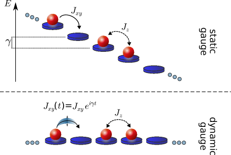
Figure 1: A schematic representation of the Stark localization problem in two gauges. The upper panel shows the static gauge, where particles are subject to a tilted potential. The bottom panel shows a dynamic gauge, where the scalar potential is written as a “vector potential,” which produces time-dependent hopping.

Theoretical arguments in favor of MBL require the localization of all the single-particle states [1, 20]. For quenched disorder this requirement is naturally satisfied in one and two-dimensional systems due to Anderson localization [21]. Various attempts to relax this requirement were performed by considering models where some of the single-particle states are delocalized [22, 23, 24, 25, 26, 27, 28, 29], as also translationally invariant models where all of the states are delocalized in the absence of interactions [30, 31, 32, 33, 34, 35, 36, 37, 38, 28]. However, the observed localization is far from being convincing and typically suffers from severe finite-size effects [36]. Moreover, while some of these models show robust localization for special initial states, most initial states are apparently delocalized [30, 28].

Anderson localization is not the only mechanism which can be used to localize the single-particle states. Single-particle states can be localized by a periodic-in-time, spatially uniform electric field at certain drive frequencies [39, 40], and also by a static uniform electric field and any field strength [41]. The former is known as dynamic localization, and the later as Wannier-Stark localization. While it was shown that dynamic localization is not stable to the addition of interactions [42], Wannier-Stark localization was argued to be stable to interactions for sufficiently strong electric fields [43, 44], a phenomenon dubbed Stark-MBL. Via a gauge change, constant electric field can be replaced by a time-dependent vector potential (see Fig. 1). Therefore the Stark problem is equivalent to a periodically driven translationally invariant interacting model; see Eq. (3). The mechanism behind Stark-MBL is currently under debate, since many of the arguments of Refs. [1, 20] cannot be readily applied due to proliferation of resonances, which are known to induce asymptotic delocalization in certain cases [45]. It was proposed that Stark-MBL follows from an approximate “shattering” of the Hilbert space due to an almost-conservation of the dipole moment [44, 46, 47]. This argument is however applicable only for an infinite electric field, $\gamma$, where jumps between sites are prohibited due to energy conservation (see Fig. 1), and cannot be easily generalized for finite and modest electric fields where the Stark-MBL transition ostensibly occurs [43, 44, 48].

The dynamics in both localized and delocalized phases was studied theoretically [43, 44, 49, 50] and experimentally [51, 52, 53] starting from special initial states. Two-dimensional systems are delocalized and show subdiffusive transport [51, 49]. For one-dimensional systems and sufficiently strong electric fields both charge-density wave (CDW) [43, 44, 52, 53] and domain-walls initial states [50] do not appear to melt completely. In fact in Ref. [50] it was argued that the system is localized in the thermodynamic limit, for any nonzero electric field, though Ref. [54] suggested that this is a special property of domain-wall initial states.

In this Letter, we consider the nonequilibrium dynamics in a one-dimensional Stark-MBL system starting from a generic initial state, which corresponds to an average over all possible initial states. We demonstrate that in both presumably delocalized, and localized regions, a local spin excitation remains localized for increasingly long times when the system size is increased, suggesting that transport might be completely suppressed only in the thermodynamic limit.

Model.—The interacting Stark model is described by the following Hamiltonian,

$$\hat{H} =\sum_{j=1}^{L-1}\frac{J_{xy}}{2}\left(\hat{S}_{j}^{+}\hat{S}_{j+1}^{-}+\text{h.c.}\right)+J_{z}\hat{S}_{j}^{z}\hat{S}_{j+1}^{z}+\sum_{j=1}^{L}W_{j}\hat{S}_{j}^{z},$$ (1)

where $L$ is the length of the spin-chain, “h.c.” denotes the hermitian conjugate, $\hat{S}_{j}^{\pm}$, $\hat{S}_{j}^{z}$ are spin-1/2 operators, $J_{xy}$ is the strength of the flip-flop term, $J_{z}$ is the strength of the Ising term, and $W_{j}=\left(\gamma j+\alpha j^{2}/L^{2}\right)$ is a spatially varying potential, where $\gamma$ corresponds to an electric field, $\alpha/L^{2}$ is the magnitude of a shallow parabolic trap that we add in order to break some of the symmetries of the system, following Ref. [43]. The system conserves the total magnetization, $\hat{M}=\sum_{j}\hat{S}_{j}^{z}$ and in the thermodynamic limit is translationally invariant (for $\alpha=0$). Through this work we use open boundary conditions and set $J_{xy}=2$, $J_{z}=1$ and $\alpha=0.5$, verifying that our results do not change qualitatively for other $\alpha$s and $J_{z}$s, as also boundary conditions (see [48]). Via the Jordan-Wigner transformation [55], the model is equivalent to a system of spinless interacting fermions moving in a uniform electric field, however for the clarity of the presentation we proceed using the spin formalism.

A number of works show an apparent ergodicity breaking for $\gamma\gtrsim 1.5$ [43, 44] (see also [48]). In this Letter, using two numerically exact methods we study spin-transport in this model.

Methods.—

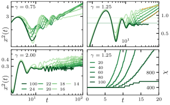
Figure 2: Mean-square displacement (MSD) as a function of time (top panels and bottom left) for $L\in[14,24]$ (Krylov based method) and $L=100$ (tDMRG). The orange dotted line correspond to power-law fits, while the horizontal lines indicate the plateau of the MSD calculated by taking the mean of the MSD between the 2nd and the 3rd peaks. The color of the plateau lines matches the coloring of the corresponding system size. Bottom right. Bond dimension, $\chi$ as a function of time obtained using tDMRG for $L\in[20,100]$ and with a fixed discarded weight $10^{-7}$. All plots were obtained for $J_{xy}=2,\ J_{z}=1$ and $\gamma=1.25$.

To assess spin-transport in the system for various electric fields, $\gamma$, we calculate the infinite temperature spin-spin correlation function,

$$G_{n}\left(t\right)=\frac{1}{\mathcal{N}}\textrm{Tr}\left[\hat{S}_{n}^{z}\left(t\right)\hat{S}_{L/2}^{z}\right],$$ (2)

where $\mathcal{N}$ is the Hilbert space dimension, and $\hat{S}_{n}^{z}\left(t\right)$ is the Heisenberg evolution of $\hat{S}_{n}^{z}$. This correlation function describes the spatial spreading of an initially local spin excitation on top of an infinite temperature state. The squared width of the excitation, is given by, $x^{2}\left(t\right)=\sum_{n}n^{2}\left(G_{n}\left(t\right)-G_{n}\left(0\right)\right)$ and is analogous to the mean-square displacement (MSD). For diffusive transport, $x^{2}\sim 2Dt$, with $D$ coinciding with the diffusion coefficient calculated from the corresponding Kubo formula [56, 57, 58, 59].

We compute $G_{n}\left(t\right)$ using two complementary numerically exact methods. In the first method we work at a zero magnetization sector, with the Hilbert space dimension $\mathcal{N}=\binom{L}{L/2}$ and utilize dynamical typicality to reduce the trace in Eq. (2) to a unitary propagation of a random initial state taken from the Haar distribution [60, 58]. We then average over a small number of such samples. Our initial condition therefore corresponds to a generic initial state with volume law entanglement. We would like to stress that while the generation of such a highly entangled pure state is probably close to impossible experimentally, we could equally well take a random product state, which can be realized experimentally. Such a state would produce an equivalent result, though it would require more averaging over the initial states to to sample the correlation function in Eq. (2).

The unitary evolution is performed using a Krylov subspace method [61]. Given the exponential scaling of the Hilbert space dimension we are able access system sizes of $L\lesssim 24$, which correspond to $\mathcal{N}\leq 2\,704\,156$, though we can propagate the system for quite long times. As a complimentary method, which provides us access to large systems sizes, we use the time-dependent density matrix renormalization group (tDMRG) [62]. In this method the wavefunction is represented as a matrix product state (MPS), built of matrices with a maximal dimension $\chi$, called the bond-dimension. The bond-dimension sets the maximum entanglement that the MPS can accommodate. If the bond dimension is set to be smaller than $\chi<d^{L/2}$, where $d$ is the local Hilbert space dimension, the error in the MPS representation of the wavefunction is bounded by the truncation weight. In our simulations, we set the truncation weight to $10^{-7}$ allowing the bond dimension to grow dynamically during the propagation. Since for ergodic systems the entanglement is typically increasing linearly with time, the computational effort increases exponentially. We checked for converges of our results by decreasing the truncation weight to $10^{-8}$. In tDMRG we use all magnetization sectors, and obtain $G_{n}\left(t\right)$ by the Heisenberg evolution of $\hat{S}_{n}^{z}\left(t\right)$, using the computational method detailed in Ref. [63]. Due to the equivalence between the ensembles of fixed and varying magnetization, in the thermodynamic limit, both Krylov based and tDMRG results are expected to agree up to some finite time when the finite size effects become important.

Results.—We calculate the MSD for a number of electric fields, $\gamma=0.75-3$ and various system sizes $L=14-24$ using the Krylov subspace method, and for sizes $L=20-100$ using tDMRG. The results are presented in Fig. 2. For times $t\leq t^{\star}\left(\gamma,L\right)$ an initial growth of the MSD is followed by a localization plateau. This plateau is visible for $\gamma\apprge 1$, and becomes even more pronounced for larger system sizes. For all the studied $\gamma$’s, including a regime where according to Refs. [43, 44] (see also [48]) the system is expected to be strongly localized, the late-time dynamics of a finite system is always delocalized, which allows us to identify the time $t^{\star}\left(\gamma,L\right)$, as the delocalization time. Note that our data suggests, that for $\gamma\apprge 1$ the system becomes localized only in the thermodynamic limit. The observed, apparently subdiffusive growth of the MSD for $t>t^{\star}\left(\gamma,L\right)$, which is consistent with previous experimental [51] and theoretical works [64, 65, 66, 54], is therefore a finite-size effect, and will not be considered further in this Letter (see however [48]). For $\gamma\leq 1$ our results are not conclusive, since the delocalization time, if it exists here, is very short, and the plateau in the MSD is not clearly visible. But, we do see that for $\gamma=0.75$ the fast growth of the MSD is pushed to later times for larger system sizes, which hints that localization at the thermodynamic limit might occur for all $\gamma>0$. A similar suggestion was recently raised in Ref. [50].

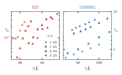
Figure 3: Delocalization time $t^{\star}$ as a function of $\gamma L$ for $\gamma=1,1.25,2,2.25$, as extracted from Krylov based method (left panel, $L\in[14,24]$) and tDMRG (right panel, $L\in[20,100]$). For all data points $J_{z}=1$.

The localization–delocalization transition at a finite time, $t^{\star}\left(\gamma,L\right)$, can also be seen from the growth of the bond-dimension in tDMRG to maintain a chosen accuracy of the results (discarded weight). For $t\leq t^{\star}\left(\gamma,L\right)$ a modest bond-dimension is required, while for $t>t^{\star}\left(\gamma,L\right)$ to keep the same accuracy of the numerical evolution an increasingly larger bond-dimension is required. We stress that the bond-dimension is not a physical quantity and we only use it as an indicator of delocalization to obtain, $t^{\star}\left(\gamma,L\right)$.

To quantitatively study the dependence of $t^{\star}\left(\gamma,L\right)$ on $\gamma$ and $L$, we extract it using two independent methods. For the Krylov subspace method it is extracted from the intersection point between two straight lines on a log-log scale: the plateau of the MSD (see caption in Fig. 2) and the apparent subdiffusive growth (dashed orange lines in Fig. 2). For tDMRG we define $t^{\star}\left(\gamma,L\right)$ as the time when the bond-dimension departs from its initial value (set to 400). While these definitions are of-course arbitrary, using different definitions did not result in a qualitative change. In Fig. 3 we show the delocalization time, $t^{\star}\left(\gamma,L\right)$ plotted vs $\gamma L$ on a semi-log scale for various tilts of the potential $\gamma$. We find that both Krylov subspace and tDMRG methods, suggest that the delocalization time increases exponentially both with $\gamma$ and $L$, namely $t^{\star}\sim\exp\left[\gamma L\right]$, such that true localization is obtained only in the thermodynamic limit. Remarkably, the tDMRG simulation of this system becomes easier, namely with the same computational resources for larger system sizes one can go to longer times. This indicates a change in the bulk dynamics, when the size of the system is increased, even though the Hamiltonian is local.

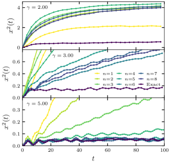
Figure 4: Mean-squared displacement as a function of time for various electric fields. The darkest lines correspond to numerically exact results obtained by using Eq. (3) for propagation. The colored lines with increasing brightness corresponds to evolution using effective Hamiltonians Eq. (4), obtained from a truncated Magnus expansion. For all panels, $J_{xy}=2,\ J_{z}=1,\ L=14$.

Magnus expansion.—In order to better understand the dependence of $t^{\star}\left(\gamma,L\right)$ on $\gamma$ we apply a time-dependent unitary transformation $\hat{U}\left(t\right)\equiv e^{-i\gamma t\sum_{j}j\hat{S}_{j}^{z}}$ to Eq. (1), which corresponds to a gauge change, replacing the potential term in Eq. (1) by a time-dependent “vector potential.” This yields the following time-dependent Hamiltonian,

$$\hat{H}\left(t\right)=\sum_{j=1}^{L-1}\left[\frac{J_{xy}}{2}\left(e^{-i\gamma t}\hat{S}_{j}^{+}\hat{S}_{j+1}^{-}+\text{h.c.}\right)+J_{z}\hat{S}_{j}^{z}\hat{S}_{j+1}^{z}\right],$$ (3)

where the electric field, $\gamma$, takes the role of a frequency. The static part of the Hamiltonian is trivially localized and has a spectrum composed of highly degenerate energy bands, which differ by a number of domain walls. It takes an energy of $J_{z}/4$ to annihilate or create a domain wall, and therefore the bands are equally spaced. The time-dependent hopping facilitates transport in the system by two possible processes: either by connecting the various bands, or by higher order, virtual transitions from some state in a band to a different state in the same band. For $\gamma\gg J_{z}/4$ both processes are suppressed since multiple spin rearrangements are required to absorb the energy of the “photon” and the system is expected to be in a long-lived prethermal state described by the time-averaged Hamiltonian (which here coincides with the static part of $\hat{H}\left(t\right)$) up to times $t^{\star}\sim\exp\left[\gamma/J_{z}\right]$ [68, 69, 70]. A slightly different scaling was suggested in Ref. [47]. We have checked that for larger $J_{z}$, the apparent localization–delocalization transition shifted to larger $\gamma$s [48].

The stroboscopic evolution of the system is determined by an effective Hamiltonian, which is defined from the one-period propagator,

$$\hat{U}\left(T\right)=\mathrm{e}^{-i\hat{H}_{\text{eff}}T}=\mathcal{T}\exp\left[-i\int_{0}^{T}\mathrm{d}\bar{t}\hat{H}\left(\bar{t}\right)\right],$$ (4)

where $\mathcal{T}$ corresponds to time-ordering, and $T=2\pi/\gamma$ is the period. For $\gamma\gg J_{z}/4$ we can approximate $\hat{H}_{\text{eff}}$ by a Magnus expansion in $\gamma^{-1}$ [71]. For $\gamma$ smaller than the many-body band-width, this expansion is not guaranteed to converge, but it can approximate the dynamics of the system up to some optimal order [72]. We use a recursive formula described in Ref. [71] to obtain $\hat{H}_{\text{eff}}$ up to order $n=10$ for $L=14$. Fig. 4 shows the stroboscopic evolution of the MSD computed numerically using $\hat{H}_{\text{eff}}^{\left(n\right)}$, which is $\hat{H}_{\text{eff}}$ truncated to an order $n$. We see that for $\gamma\leq 2$ the Magnus expansion fails to approximate the dynamics even for short times, while for $\gamma=3,5$ as the Magnus order $n$ increases, the approximate solution approaches the exact solution for longer times (it is hard to reliably extract $t_{\text{magnus}}$ from our data to obtain the functional dependence on $n$, but see Ref. [73]). There is little to no dependence of $t_{\text{magnus}}$ on the system size (see [48]). Interestingly, the long times dynamics of $\hat{H}_{\text{eff}}^{\left(n\right)}$ is diffusive with a diffusion coefficient which decreases with $n$ [48], even for $\gamma=5$, where the system is expected to be strongly localized [43, 44].

Discussion.—In this Letter, using two complementary numerically exact methods, we have examined the dynamics of a spin-excitation starting from a generic initial condition in a spin-chain which is expected to exhibit Stark-MBL. For $\gamma>J_{z}$ we find strong evidence of a finite delocalization time, $t^{\star}\left(L,\gamma\right)$, which scales exponentially with both the size of the system and the electric field, namely $t^{\star}\left(L,\gamma\right)\sim\exp\left[\gamma L/J_{z}\right]$. For intermittent times $t<t^{\star}$ the spin-excitation is localized, while for $t>t^{\star}$ it delocalizes in a manner consistent with subdiffusion [51]. This strongly suggests that for $\gamma\apprge J_{z}$, Stark-MBL strictly occurs only in the thermodynamic limit, $L\to\infty$, while any finite system is ultimately delocalized for sufficiently long times. For $\gamma\leq J_{z}$ and system sizes and times accessible to us, the localization regime is not apparent. Nevertheless, we do see that the dynamics is delayed with increasing the system size, which can be consistent with a localization length larger than the system size $\xi\left(\gamma\right)\gg L$. It is therefore plausible to conjecture that that Stark-MBL in the thermodynamic limit occurs for all $\gamma>0$, which is consistent with the conjecture in Ref. [50].

In the dynamic gauge, where the electric field is replaced by a periodically driven flip-flop term such that $\gamma$ plays the role of the frequency, it is rigorously known that for $\gamma\gg J_{z}$ the heating time is exponential in $\gamma/J_{z}$ [68, 69, 70]. We show that for sufficiently large electric fields, up to time $t_{\text{magnus}}$, the dynamics is well approximated by a static effective Hamiltonian obtained from a Magnus expansion truncated up to order $n$. This time increases with both $\gamma/J_{z}$ and $n$ (cf. Ref. [73]). The first order of the expansion is given by $\hat{H}_{\text{eff}}^{\left(1\right)}=J_{z}\sum_{j=1}^{L-1}\hat{S}_{j}^{z}\hat{S}_{j+1}^{z}+O\left(J_{z}/\gamma\right)$. The spectrum of $\hat{H}_{\text{eff}}^{\left(n\right)}$ is composed of equally space bands, $J_{z}/4$ distance apart, with a bandwidth of $O\left(J_{z}/\gamma\right)$ [48]. Therefore, for $\hat{H}_{\text{eff}}^{\left(n\right)}$ the situation is similar to models of quasi-MBL, which show asymptotic delocalization [33, 36, 45]. Indeed all $\hat{H}_{\text{eff}}^{\left(n>1\right)}$ show diffusion at long times, with a diffusion constant decreasing with $n$ [48]. We would like to stress that the delocalization of $\hat{H}_{\text{eff}}^{\left(n\right)}$ occurs before the delocalization in Eq. (1) and Eq. (3) at time $t^{\star}$, and therefore Magnus expansion does not capture the delocalization regime of Eq. (1) and Eq. (3). It does suggest that the localization mechanism of Stark-MBL is probably different from Floquet-MBL, where the effective Hamiltonian is expected to be non-ergodic [16, 18].

While the analysis we provided explains the transient localization regime, it does not explain why the delocalization time increases with the size of the system, suggesting that Stark-MBL happens only in the thermodynamic limit. This conclusion remains qualitatively robust for both open and periodic boundary conditions, in the static and dynamic gauges, and with and without the parabolic potential in Eq. (1) [48]. A possible explanation could be that the measure of delocalized states is vanishing in the thermodynamic limit. This would also explain why localization appears to be robust for CDW and domain-wall initial states. We leave the exploration of this avenue to future studies.

Supplementary Material: Transport in Stark Many Body Localized Systems

I Transition location

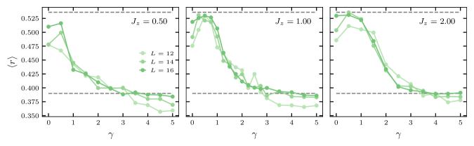
Figure S1: $\left\langle r\right\rangle$ as of a function of electric field strength for various interaction strengths (different panels), and system sizes. Larger system size corresponds to stronger color intensity. The black dashed lines correspond to WD statistics ($r\simeq 0.536$) and Poisson ($r\simeq 0.39$) statistics. The model parameters that were used are $J_{xy}=2,\ J_{z}\in[0.5,1,2],\ \alpha=0.5$.

To approximately assess the location of the Stark-MBL transition we use the standard metric,

$$r_{\alpha}=\text{min}\left(\frac{s_{\alpha}}{s_{\alpha-1}},\frac{s_{\alpha-1}}{s_{\alpha}}\right),$$ (S1)

where $s_{\alpha}\equiv E_{\alpha+1}-E_{\alpha}$ are the spacing between adjacent eigenvalues of the Hamiltonian. For integrable systems the mean of this quantity ($\left\langle r\right\rangle$), is typically given by $\left\langle r\right\rangle\approx 0.39$, which corresponds to a Poissonian distribution, while for quantum chaotic systems it is $\left\langle r\right\rangle\approx 0.536$, which corresponds to Wigner Dyson distribution. In Fig. S1 we examine $\left\langle r\right\rangle$ as a function of the electric field strength $\gamma$ for various couplings $J_{z}$. We observe a transition from a Wigner-Dyson distribution for low electric fields to a Poissonian distribution at high electric fields. The transition occurs approximately at $\gamma\approx J_{z}$. This analysis does not depend strongly on the size of the system, in contrast to the mean-square displacement results presented in the main text. The middle panel ($J_{z}=1$) is in agreement with Ref. [44] although we have used a different mechanism to break the symmetries of the model.

II Delocalization time extraction

In Fig. S2 we present the analysis used to obtain $t^{\star}\left(\gamma,L\right)$ in Fig. 3 in the main text. The mean-square displacement (MSD) shows severe finite size effects, with subdiffusive behavior delayed to later times for larger system sizes. The locations of the plateaus (green horizontal lines) are calculated by taking the mean of the MSD between the 2nd and the 3rd peaks of the MSD. We fit the late time behavior with a power-law fit, $x^{2}\propto t^{a}$ (orange dashed lines), and estimate the delocalization time $t^{\star}\left(\gamma,L\right)$ by the intersection of the plateaus with the power-law fits (orange crosses).

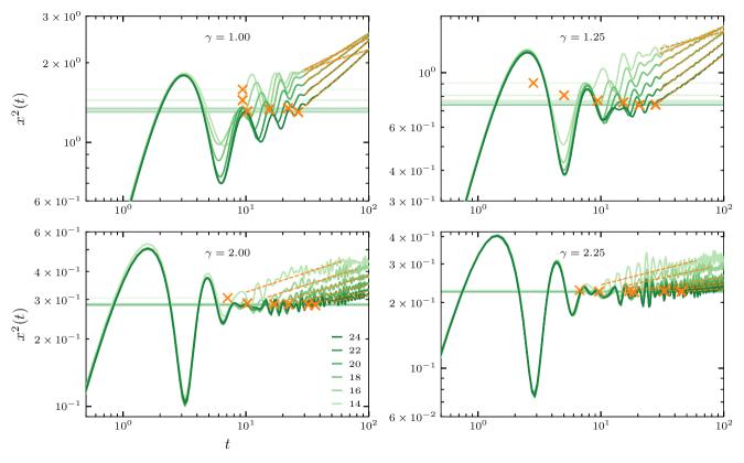
Figure S2: Mean-square displacement (MSD) as a function of time for $L\in[14,24]$ (Krylov based method). The orange dashed line correspond to power-law fits ($x^{2}\sim t^{a}$), while the horizontal lines indicate the plateau of the MSD calculated by taking the mean of the MSD between the 2nd and the 3rd peaks. The orange crosses are the estimated delocalization time $t^{\star}\left(\gamma,L\right)$ obtained from the intersection of the power-law fits with the plateau. The color of the plateau lines matches the coloring of the corresponding system size. All plots were obtained using $J_{xy}=2,\ J_{z}=1$.

III Finite-size subdiffusive behavior

From the power law-fits in Fig. S2 we can obtain the dynamical exponent $a$, which corresponds to the late-time growth of the MSD, $x^{2}\sim t^{a}.$ We plot this exponent as a function of the electric field $\gamma$ and for various system sizes in Fig. S3. One can see an apparent transition between a subdiffusive behavior ($a<1$) to a localized behavior ($a\sim 0$), with very strong finite-size effects.While for $\gamma>J_{z}$ the exponent seems to converge with the size of the system, it is important to keep in mind that the onset of the subdiffusive transport is pushed to later times for larger system sizes, as one can see in the main text and in Fig. S2 indicating that the observed subdiffusive behavior is a finite-size effect.

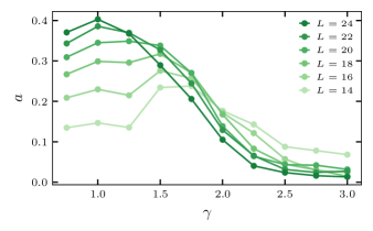
Figure S3: The dynamical exponent $a$ as obtained from the fits to the MSD, $x^{2}\propto t^{a}$ (see Fig. S2), as function of $\gamma$ for various system sizes ($L\in[14,24]$).

IV Sensitivity to boundary conditions

In this Section we show that the conclusions of the main text are robust to changes in the gauge and the boundary conditions. In Fig. S4 we have calculated the MSD as a function of time, using the dynamical gauge, (3) in the main text for various electric fields $\gamma$ (rows), various system sizes (color intensity), and two different boundary conditions (columns). We see that in the dynamic gauge the MSD shows less pronounced oscillations compared to the static gauge, allowing to spot the formation of the localization plateau already for $\gamma=1.$ The results remain qualitatively the same to the results in the static gauge (Fig.S2), with severe finite size effects, and a delocalization time that is increasing with the system size. The quantitative difference between open and periodic boundary conditions serves as another indication of finite-size effects, though the localization plateau for both boundary conditions appears at about the same MSD.

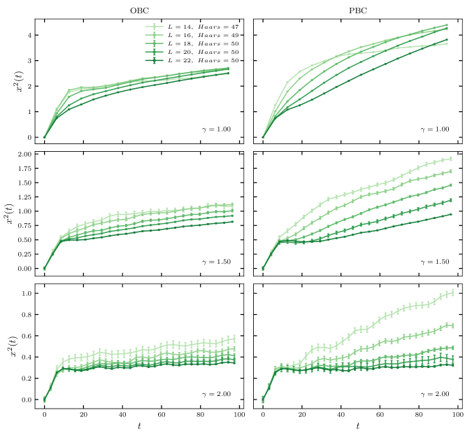
Figure S4: Mean-square displacement (MSD) as a function of time for $L\in[14,24]$ (Krylov based method) calculated from the dynamic gauge (3) in the main text. Left column: open boundary conditions (OBC). Right column: periodic boundary conditions (PBC). Different rows have different electric fields $\gamma\in[1,1.5,2]$. All plots were obtained for $J_{xy}=2,\ J_{z}=1$.

V Dynamical behavior of truncated effective Hamiltonians

In this Section we study the late-times dynamical behavior of the effective Hamiltonians calculated using Magnus expansion in $\gamma^{-1}$ up to some order $n$. In Fig. S5 (left column) we calculate the MSD for two electric fields (rows). We see that it develops a pronounced linear behavior, indicative of diffusion, $x^{2}\sim 2Dt$, where $D$ is the linear response diffusion coefficient. For even longer times the MSD saturates, since the system is finite. We extract the diffusion coefficient from the relevant time windows (black dashed lines in Fig. S5), and plot it as a function of the truncation order, $n$ on the right column of Fig. S5.

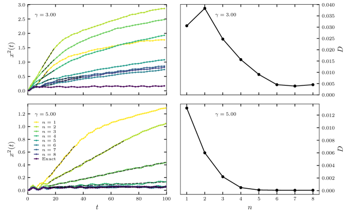
Figure S5: Mean-squared displacement as a function of time for two electric fields (left column). The darkest lines correspond to numerically exact results obtained using (Eq. 3 in the main text). The colored lines with increasing intensity corresponds to evolution using effective Hamiltonians (S2), obtained from a truncated Magnus expansion. The black dashed lines corresponds to linear fits, $x^{2}\sim 2D\,t$, and the diffusion coefficient $D$ is plotted in the right column as function of the truncation order. For both $\gamma=3,5$ there is a visible trend of $D\propto 1/n$. The parameters used are, $J_{xy}=2,\ J_{z}=1,\ L=14$.

The diffusion coefficient $D\left(\gamma,n\right)$ is monotonically decreasing with the order of the Magnus expansion and the strength of the electric field, approximately following $D\sim 1/n$. While this finding indicates that the truncated effective Hamiltonian is delocalized, it doesn’t imply much on the original interacting Stark model, since the diffusive behavior of the effective Hamiltonian emerges for at times for which the dynamics under the effective Hamiltonian doesn’t not well approximate the numerically exact dynamics. What is interesting, is that the infinite order Magnus expansion, if it is convergent, could correspond to localized dynamics.

VI Convergence criteria of the Magnus expansion

In this Section we examine the convergence of the Magnus expansion of the effective Hamiltonian,

$$\hat{H}_{\text{eff}}^{\left(n\right)}=\sum_{k=0}^{n}\hat{H}_{k},$$ (S2)

while each term $\hat{H}_{k}$ is of the order of $\gamma^{-k}$. The D’Alembert criterion of convergence is $\left\|\hat{H}_{k+1}\right\|/\left\|\hat{H}_{k}\right\|<1$, where $\left\|.\right\|$ indicates the operator norm. In Fig. S6 we the D’Alembert criterion is presented for different electric fields, $\gamma$. We see that while for $\gamma\leq 2$ the series is divergent, for $\gamma\apprge 3$ is it convergent at least up to 10th order. We note that this doesn’t necessarily mean that the series has a finite radius of convergence, since divergence can occur for relatively large expansions orders [73].

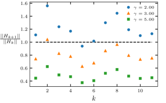
Figure S6: D’Alembert criterion of convergence as a function of the Magnus expansion order ($k$), $\left\|\hat{H}_{k+1}\right\|/\left\|\hat{H}_{k}\right\|<1$ (see (S2) for definition). Different colors (markers) represents different electric field strength $\gamma=2,3$ and 5. The dashed black line corresponds to a convergence requirement.. The parameters used are, $J_{xy}=2,\ J_{z}=1,\ L=10$.

VII Density of states of the truncated effective Hamiltonians

The zero order truncated effective Hamiltonian, $\hat{H}_{\text{eff}}^{\left(0\right)}$ in (S2) corresponds to the interaction term,

$$\hat{H}_{\text{eff}}^{\left(0\right)}=J_{z}\sum_{i=1}^{L}\hat{S}_{i}^{z}\hat{S}_{i+1}^{z},$$ (S3)

whose spectrum is composed of equally spaced degenerate bands, separated $J_{z}/4$ apart. The following terms of the expansion are of order $J_{z}/\gamma$, and they partially lift this degeneracy giving a width of $J_{z}/\gamma$ to the bands. To demonstrate this in Fig. S7 we plot the density of states (DOS) of $\hat{H}_{\text{eff}}^{\left(n\right)}$ for a number of electric fields, $\gamma$. While the gaps are washed away for $J_{z}/4<J_{z}/\gamma$, namely $\gamma<4$, they become clearly visible as $\gamma$ increases.

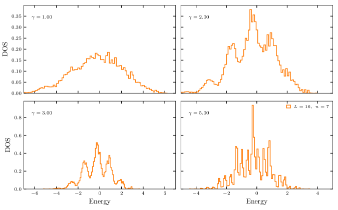
Figure S7: The density of states of the truncated effective Hamiltonian $\hat{H}_{\text{eff}}^{\left(n=7\right)}$ for $L=16$ and $\gamma=1,2,3$ and 5$5$. .All plots were obtained for $J_{xy}=2,\ J_{z}=1$.

VIII Finite-size analysis

In Fig. S8 we repeat the analysis of Fig. 4 from the main text for a number of system sizes, showing that there are no considerable system size dependence in the determination of $t_{\text{Magnus}}$, namely the time up to which there is a reasonable agreement between the MSD computed using $\hat{H}_{\text{eff}}^{\left(n\right)}$ and the MSD of the dynamical gauge Hamiltonian (3) in the main text.

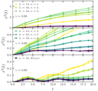
Figure S8: Finite size analysis of Fig. 4 in the main text. Mean-squared displacement as a function of time for various electric fields. The darkest lines correspond to numerically exact results obtained using (Eq. (3) in the main text). The colored lines corresponds to an evolution using the effective Hamiltonian (S2), obtained from a truncated Magnus expansion. Different markers ($\CIRCLE$, $\blacktriangle$, $\blacksquare$) stand for different system sizes $L=14,16$ and 18, correspondingly. The used parameters are, $J_{xy}=2,\ J_{z}=1$.