The impact of the FMR and starburst galaxies on the (low-metallicity) cosmic star formation history

Abstract

The question how much star formation is occurring at low metallicity throughout the cosmic history appears crucial for the discussion of the origin of various energetic transients, and possibly - double black hole mergers. We revisit the observation-based distribution of birth metallicities of stars (f_SFR(Z,z)), focusing on several factors that strongly affect its low metallicity part: (i) the method used to describe the metallicity distribution of galaxies (redshift-dependent mass metallicity relation - MZR, or redshift-invariant fundamental metallicity relation - FMR), (ii) the contribution of starburst galaxies and (iii) the slope of the MZR. We empirically construct the FMR based on the low-redshift scaling relations, which allows us to capture the systematic differences in the relation caused by the choice of metallicity and star formation rate (SFR) determination techniques and discuss the related f_SFR(Z,z) uncertainty.
We indicate factors that dominate the f_SFR(Z,z) uncertainty in different metallicity and redshift regimes. The low metallicity part of the distribution is poorly constrained even at low redshifts (even a factor of $\sim$200 difference between the model variations) The non-evolving FMR implies a much shallower metallicity evolution than the extrapolated MZR, however, its effect on the low metallicity part of the f_SFR(Z,z) is counterbalanced by the contribution of starbursts (assuming that they follow the FMR). A non-negligible fraction of starbursts in our model may be necessary to satisfy the recent high-redshift SFR density constraints.

1 Introduction

The observed populations of stars, their remnants and related transients consist of objects formed at different times and with different metallicities. To model those populations and to correctly interpret observations, it is necessary to know the metallicity dependent star formation history (SFH) of the observed galaxy, galaxies in the probed volume, or even of the entire Universe. Knowledge of the latter - which is the subject of interest of this study - becomes increasingly important in the era of gravitational wave (GW) astrophysics. That is because the time between the formation of the progenitor stars and merger of stellar black holes or neutron stars observed in GW can be comparable to the age of the Universe (e.g. Belczynski et al., 2016). Moreover, the efficiency of formation of merging binaries may show a strong metallicity dependence. In particular, it has been suggested that double black hole mergers may form much more efficiently in low metallicity environments ($\lesssim$0.1 solar metallicity; e.g. Klencki et al., 2018; Giacobbo et al., 2018). This makes the modelled properties of the population of such systems particularly sensitive to the assumed distribution of the cosmic star formation rate density (SFRD) at different metallicities and redshifts, f_SFR(Z,z) (e.g. Chruslinska et al., 2019; Neijssel et al., 2019; Broekgaarden et al., 2021) and requires knowledge of f_SFR(Z,z) even beyond the peak of the cosmic SFH. To confront the model predictions with observations and draw correct conclusions from such a comparison, it is necessary to take into account the f_SFR(Z,z) uncertainty, which may be substantial - especially at high redshifts (Chruslinska & Nelemans, 2019; Chruślińska et al., 2020; Boco et al., 2021). Given the many uncertain pieces of information that need to be combined to estimate f_SFR(Z,z), an (observation-based) determination of this distribution presents a challenge in itself. In this study we take a closer look at two of those pieces: the empirical correlation between the star formation rate and metallicity of star forming galaxies (the so-called fundamental metallicity relation, e.g. Ellison et al. 2008; Mannucci et al. 2010) and the contribution of starburst galaxies. We build on the observation-based f_SFR(Z,z) model from Chruslinska & Nelemans (2019) (briefly introduced in Sec. 2) and expand the discussion presented in Boco et al. (2021), aiming to evaluate the uncertainty (or - find realistic, observationally allowed extremes) of the metallicity dependent cosmic SFH in view of those factors. Where appropriate we adopt a standard flat cosmology with $\Omega_{M}$=0.3, $\Omega_{\Lambda}$=0.7 and H₀=70 km s^-1 Mpc^-1, assume a (universal) Kroupa (2001) initial mass function (IMF) and solar metallicity of 12 + log₁₀(O/H)_⊙=$Z_{O/H\odot}$=8.83 and ${\rm~{}Z}_{\odot}=0.017$ (Grevesse & Sauval, 1998).

2 An observation based $f_{SFR}(Z,z)$ determination

We construct f_SFR(Z,z) building on the framework detailed in Chruslinska & Nelemans (2019). In essence, their method is based on a combination of three key ingredients: the distribution of galaxy stellar masses (galaxy stellar mass function - GSMF), and the distributions describing the star formation rates (SFR) and metallicities of galaxies at fixed stellar mass $M_{*}$. All distributions are redshift-dependent. The GSMF is used to obtain the number density of galaxies of different masses. The contribution of galaxies of different masses to the total SFRD can then be obtained by weighing the number density of galaxies in a given mass range by their SFR. Finally, f_SFR(Z,z) is obtained by assigning a metallicity to each $M_{*}$.
The SFR and metallicity distributions are modelled as log-normal distributions centered on the empirical star formation-mass relation (SFMR) and the mass - (gas-phase) metallicity relation (MZR) respectively, with dispersions $\sigma_{\rm SFMR}$ and $\sigma_{\rm MZR}$ (representing the intrinsic scatter around the two relations). Note that the observational gas-phase metallicity estimates probe the oxygen abundance ($Z_{O/H}$=12+log₁₀(O/H)), and that is the metallicity measure used in our study. Additional scatter in $Z_{O/H}$ is introduced to model the spread in the metallicity at which the stars are forming within the galaxies. To determine all the necessary ingredients, the authors assemble a compilation of observational results describing the MZR, SFMR and GSMF, combined over a wide range of redshifts ($z$) and $M_{*}$. Several variations of the base relations (SFMR, MZR, GSMF) are explored in order to discuss the impact of the uncertain absolute metallicity scale (steming from the differences between the estimates obtained with different metallicity determination methods), the shape of the high mass end of the SFMR and the redshift evolution of the low mass end of the GSMF (see Sec. 2 in Chruslinska & Nelemans 2019 and references therein)
In this study we explore an alternative method to obtain the redshift-dependent metallicity distribution of star forming galaxies, based on the fundamental metallicity relation. We then modify the SFR distribution to better account for the contribution of star forming galaxies that are strong outliers to the general SFMR (starbursts). Our motivation for those modifications and the details of our approach are laid out in Sec. 3 and Sec. 4 respectively.

3 The fundamental metallicity relation

The fundamental metallicity relation (FMR) is a three parameter dependence linking M_∗, SFR and gas phase metallicity of star forming galaxies (Ellison et al., 2008; Mannucci et al., 2010). The relation implies the mass-metallicity correlation, as observed in the MZR, but it also introduces an anti-correlation between metallicty and SFR, such that galaxies of the same stellar mass showing higher than average SFR also have lower metallicities (i.e. the galaxy’s offset from the average mass-metallicity relation -MZR- is anti-correlated with its offset from the average SFR-mass relation).
The existence of such SFR-metallicity anti-correlation has been reported in numerous observational studies (e.g. Mannucci et al., 2011; Yates et al., 2012; Andrews & Martini, 2013; Bothwell et al., 2013; Lara-López et al., 2010; Salim et al., 2014; Zahid et al., 2014b; Yabe et al., 2015; Hunt et al., 2016; Sanders et al., 2018; Cresci et al., 2019; Curti et al., 2020; Sanders et al., 2020) and established up to redshift $z\sim 3.5$.
Such correlation is also expected from theoretical models of galaxy evolution and is thought to reflect the changes in the SFR-fuelling gas fraction present within the galaxy (e.g. Ellison et al., 2008; Davé et al., 2011; Yates et al., 2012; De Lucia et al., 2020). Lower SFR for a given M_∗ then implies that the galaxy has already used up most of its cold gas reservoir (fuelling its SFR in the past), and therefore (in the absence of strong outflows) its interstellar medium is more metal rich than that of the galaxy of the same mass that is still highly star forming. At low SFR there are also fewer supernovae that can remove (especially at low M_∗) metal rich gas from the galaxy. In turn, inflowing metal poor material lowers the metallicity and provides additional fuel for the SFR, increasing the latter. As long as the time-scales on which the SFR and metallicity evolve are of the same order, the anti-correlation between the galaxy offsets from the MZR and SFMR is expected to hold (e.g. Torrey et al., 2018). Those timescales are similar for the feedback/SFH implementations used in the large-scale cosmological simulations such as EAGLE and Illustris-TNG, which warrants the existence of the FMR up to high redshifts in the simulations (Lagos et al., 2016; De Rossi et al., 2017; Torrey et al., 2018). However, Torrey et al. (2018) point out that the strength of the correlation - especially for low mass galaxies at high redshift - may be reduced if models with particularly strong and/or bursty feedback are used. Lagos et al. (2016) find that the shape of the FMR in the EAGLE simulations depends on the adopted model of star formation. Therefore, observational confirmation of the existence or breakdown of the FMR at high redshifts will help to discriminate between the different feedback and star formation prescriptions.
Observationally, the FMR is found to show little to no evolution with redshift up to z$\sim$3 within the uncertainty of the current data and range of galaxy properties probed (see Cresci et al. 2019 and Sanders et al. 2020 for recent discussion). Since both the mass and SFR distributions of star forming galaxies change over time, the apparent lack of FMR evolution implies that galaxies at different redshifts probe different parts of the locally established relation. At fixed M_∗, a decrease in the average galaxy metallicity as a function of redshift is still expected, as the typical SFR is higher at earlier cosmic times.

At $z\gtrsim 2$, the rate of decrease in metallicity implied by a non-evolving FMR is much weaker than that reported by various studies discussing the redshift evolution of the MZR (e.g. Maiolino et al., 2008; Mannucci et al., 2009). Similarly to the FMR, the MZR (and its evolution with redshift) is virtually unconstrained at redshifts $z\gtrsim 3.5$ (Maiolino & Mannucci, 2019). This uncertainty in the rate of metallicity evolution is one of the key factors affecting the f_SFR(Z,z). In particular, different high redshift extrapolations of empirical relations used in the literature lead to drastically different conclusions about the birth metallicities of stars forming beyond the peak of the cosmic SFH (e.g. Chruslinska et al., 2019; Chruslinska & Nelemans, 2019; Boco et al., 2021).
Recent observational studies find support for rapid early metal enrichment in high redshift galaxies, pointing towards a weak MZR evolution that is more in line with the apparently invariant FMR (see Sec. 3 in Boco et al. 2021 and references therein for a recent discussion). Such weaker metallicity evolution is also in agreement with the results of cosmological simulations and semi analytical models of galaxy evolution (e.g. Yates et al., 2012; Torrey et al., 2019). Furthermore, Sanders et al. (2020) show that when the differences in the properties of the ionized gas within HII regions (responsible for the emission lines used to estimate the metallicity; in particular lower iron to oxygen ratio for the same O/H found in high redshift galaxies) of galaxies at different redshifts are taken into account, the inferred MZR evolution is milder (i.e. metallicities of high redshift galaxies are biased low if those differences are neglected). In fact, the MZR evolution found by Sanders et al. (2020) is consistent with the non- or weakly evolving FMR within the redshift and mass range probed in their study. The existence of a FMR also means that if the galaxy sample is biased towards high SFRs, the inferred average metallicity is underestimated. Such biases can be expected in high redshift and low stellar mass galaxy samples, affecting the MZR shape (the low mass end slope) and the rate of evolution with redshift (a decrease in the normalisation).

In light of the above discussion, we conclude that the assumptions about the metallicity evolution made in Chruslinska & Nelemans (2019), which rely on the MZR obtained by Mannucci et al. (2009) and extrapolate its redshift evolution based on their two highest redshift bins, are likely to overestimate the rate of metallicity decrease at $z\gtrsim 2$ and require revision: either assuming a weaker MZR evolution, or using the FMR to assign metallicity to galaxies.
The use of the FMR instead of a MZR in f_SFR(Z,z) determination appears advantageous for two reasons: (i) the redshift invariance of the FMR allows to circumvent the problem of the uncertain MZR evolution with redshift - the metallicity distribution at each $z$ is then defined by the local FMR and the SFMR and GSMF (whose $z$ dependence is generally better constrained than that of the MZR). We stress that with the current data there is no guarantee that at z$\gtrsim$3 the FRM remains (close to) redshift invariant. By assuming a non-evolving FMR throughout the entire cosmic history we explore another extreme assumption (with respect to Chruslinska & Nelemans (2019)) about the rate of metallicity evolution at high redshift. (ii) if all star forming galaxies follow the FMR (at present, there is no clear evidence to the contrary), it can be used to describe metallicity of galaxies belonging to populations for which there are little examples of metallicity determinations (e.g. strong outliers of the star forming main sequence that are not described by the MZR, such as starburst galaxies, see Sec. 4).

However, the major problem with this approach is that there is no agreement on the exact form of this three parameter mass-SFR-metallicity dependence. The f_SFR(Z,z) derived with the FMR will necessarily strongly depend on the choice of this relation, just as it strongly depends on the choice of MZR and its extrapolated evolution. While the discussion of the systematic effects on the f_SFR(Z,z) introduced by the choice of a particular form of the MZR is relatively straightforward (Chruslinska & Nelemans, 2019) and to a large extent boils down to the discussion of differences caused by the use of different metallicity determination methods (which are well documented in the literature, e.g. Kewley & Ellison 2008, Maiolino & Mannucci 2019), an analogous discussion for the FMR is not. The observationally inferred FMR is known to non-trivially depend on the metallicity determination method, the SFR determination method and the galaxy sample selection criteria (e.g. Yates et al., 2012; Hunt et al., 2016; Kashino et al., 2016; Telford et al., 2016; Cresci et al., 2019). We note that it is not clear how the FMR depends on each of those factors. Therefore, one needs to be cautious when using different literature results concerning the properties of galaxy populations (e.g. the SFMR) in combination with a particular FMR estimate - if those results are based on different techniques, this would represent an internally inconsistent approach.
Instead of using a particular example from the literature, in our analysis we resort to a phenomenological description of the FMR. We aim to capture the robust observational/theoretical features of the mass-SFR-metallicity dependence and describe the variations in the shape of this dependence caused by different choices of the local MZR and SFMR (that reflect the differences in the metallicity and SFR determination methods used in the literature). This allows us to ensure the consistency of the method and discuss the realistic extremes of the f_SFR(Z,z).

3.1 Constructing the FMR from $z\sim 0$ scaling relations

To construct our model FMR, we describe its 2D projection on the Z_O/H-log₁₀(M_∗) plane. This projection is the most commonly shown in observational studies. We refer to it as $Z_{O/H}(SFR,M_{*})$ (see Fig. 1 for the illustration).
At fixed SFR, the shape of Z_O/H(SFR,M_∗) is found to show the same characteristic features as the MZR: the low mass part of the relation is almost linear (Z_O/H $\propto$ log₁₀(M_∗), it bends around a certain turnover mass and flattens at high masses, approaching a constant metallicity value (see e.g. Mannucci et al. 2010, 2011; Yates et al. 2012; Andrews & Martini 2013; Hunt et al. 2016; Telford et al. 2016; Cresci et al. 2019; Curti et al. 2020; Sanders et al. 2020). To describe this dependence, we use the parametrisation from Curti et al. (2020):

$$\rm Z_{O/H}(SFR,M_{*})=Z_{O/H;0}-\frac{\gamma}{\beta}log\left(1+(\frac{M_{*}}{M_{0;SFR}})^{-\beta}\right)$$ (1)

where $Z_{O/H;0}$ is the asymptotic metallicity of the high-mass end of the relation, $M_{0;SFR}$ is the turnover mass, $\gamma$ is the slope of $Z_{O/H}(SFR,M_{*})$ at $M_{*}<<M_{0;\rm SFR}$ and $\beta$ regulates the width of the knee of the relation. The $Z_{O/H}(SFR,M_{*})$ dependence on SFR is expected primarily in the turnover mass $M_{0;\rm SFR}$, as illustrated in the right panel of Figure 1. The left panel of Figure 1 illustrates the average $z\sim 0$ MZR and SFMR. We relate the $Z_{O/H}(SFR,M_{*})$ parameters to those of the average $z\sim 0$ scaling relations - each of the parameters of eq. 1 is discussed in the relevant subsection below. Discussion of the observational properties of the $Z_{O/H}(SFR,M_{*})$ in the reminder of this section and our choices are motivated by the results shown in the references given at the beginning of this section - we do not list them again in each of the subsections, unless we refer to a result from a specific paper(s).

Equation 1 describes the shape of the relation, but the main observable property that characterizes the FMR is the quantity that relates the galaxy’s offset from the average MZR and SFMR (i.e. quantifies the strength of the SFR-metallicity correlation). To describe the strength of the SFR-metallicity correlation we introduce the coefficient $\nabla_{\rm FMR}$, defined as follows:

$$\delta_{MZR}=-\nabla_{FMR}\cdot\delta_{SFMR}$$ (2)

where $\delta_{MZR}$ = Z_O/H,gal. - Z${}_{O/H,at\ MZR}$ and $\delta_{SFMR}$ = log₁₀(SFR_gal.) - log₁₀(SFR${}_{at\ SFMR}$) are the galaxy’s offsets from the average MZR and SFMR . Higher values of $\nabla_{\rm FMR}$ imply a stronger correlation.

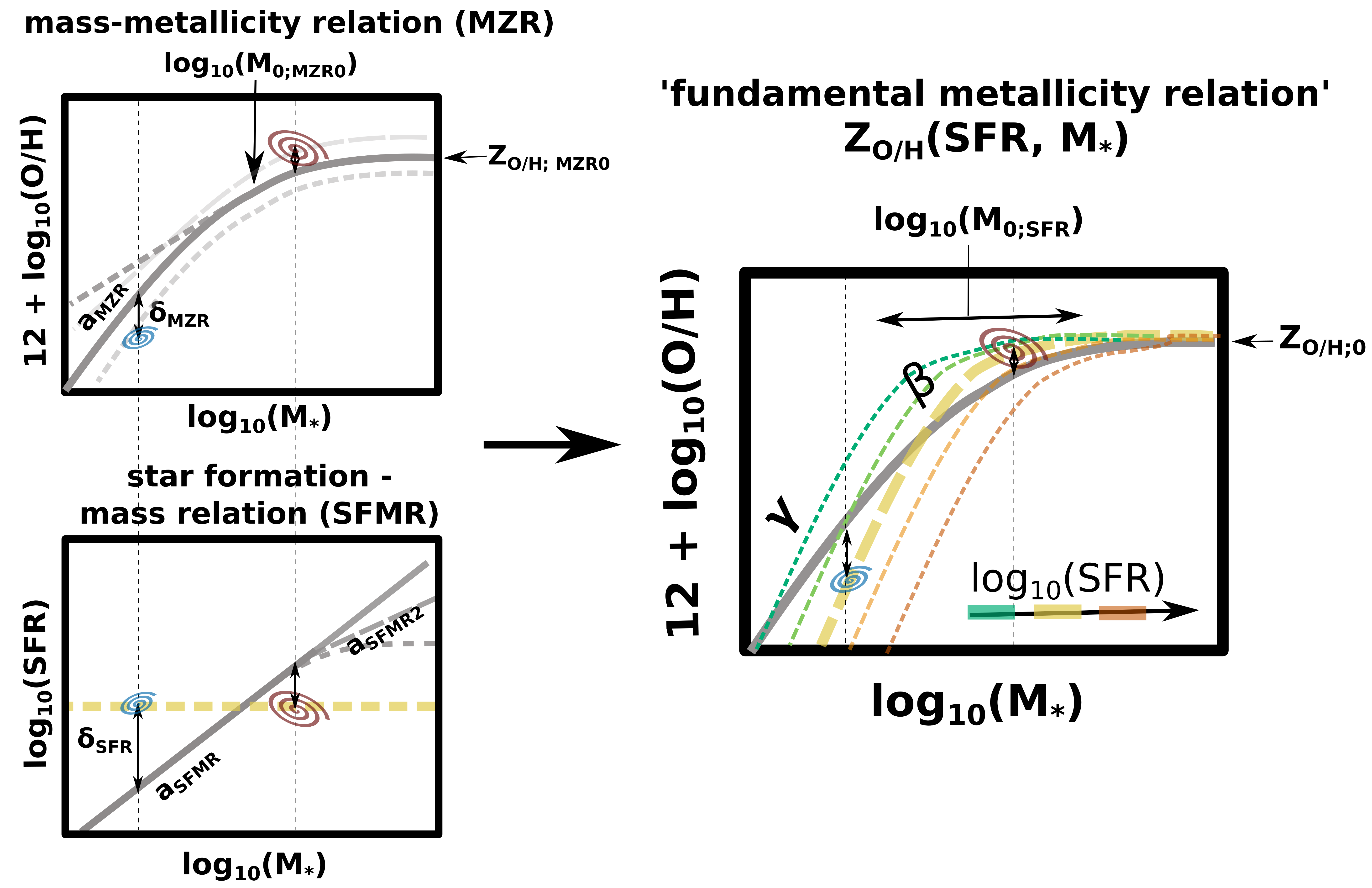
Figure 1: Sketch illustrating the local MZR (top left), SFMR (bottom left) and the three parameter mass-metallicity-SFR dependence Z_O/H(SFR, M_∗) (right), indicating the key parameters of those relations and the observed anti-correlation between the galaxy’s offsets from the MZR ($\delta_{MZR}$) and SFMR ($\delta_{SFMR}$). We consider different assumptions about the MZR and SFMR relations (i.e. normalization $\rm Z_{O/H;MZR0}$ and slope $a_{\rm MZR}$ of the MZR, high mass end of the SFMR $a_{SFMR2}$) to cover the range of possibilities present in the literature, as indicated with the thick gray lines in the left panels. In Sec. 3.1 we relate the parameters of the Z_O/H(SFR, M_∗) to the parameters of the local 2D relations.

3.1.1 The asymptotic metallicity

A clear feature present among the observational $Z_{O/H}(SFR,M_{*})$ determinations is the high mass flattening. We note that some authors report a reversal of the (anti-)correlation at high M_∗ rather than a simple flattening, e.g. Yates et al. 2012; Kashino et al. 2016). Telford et al. (2016) point out that certain sample selection criteria (e.g. applying signal to noise ratio cuts on oxygen lines used to estimate the metallicity) may lead to biases against the massive, low SFR galaxies and therefore affect the inferred low SFR and high mass part of the FMR. They argue for such biases as the cause of the reversal of the correlation at high masses as seen in Kashino et al. (2016). The effects of dust (and the applied dust SFR corrections) may also induce biases against massive, metal rich galaxies (Telford et al., 2016).
Change in the relation at high masses is also supported theoretically, and could be attributed to the increased importance of AGN feedback that can rapidly influence the SFR while the metallicity continues to evolve much more gradually (e.g. De Rossi et al., 2017; Torrey et al., 2018). We therefore assume that the high mass flattening is a robust feature of the $Z_{O/H}(SFR,M_{*})$ and include it within our model. Observationally, the value of the asymptotic metallicity $Z_{O/H;0}$ at which the relation flattens appears to be roughly independent of the SFR and coincide with that of asymptotic metallicity of the average z$\sim$0 MZR ($Z_{O/H;MZR0}$). As such, it is affected by the choice of the metallicity determination method, which leads to systematic offsets in the normalisation of the MZR (compare examples shown in Telford et al. 2016 and in Fig. 2 in Cresci et al. 2019).
We fix $Z_{O/H;0}=Z_{O/H;MZR0}$, where $Z_{O/H;MZR0}$ is defined by the choice of the $z\sim 0$ MZR.

3.1.2 The slope at low masses and high SFR

At the low mass end, the Z${}_{O/H}(SFR,M_{*})$ for fixed log₁₀(SFR) seems to be well approximated with a linear dependence. Accordingly, in this regime ($M_{*}<<M_{0;SFR}$), eq. 1 reduces to:

$$\rm Z_{O/H}(SFR,M_{*})=Z_{O/H;0}+\gamma log_{10}\left(M_{*}\right)-\gamma log_{10}\left(M_{0;SFR}\right)$$ (3)

The slope of this dependence is generally steeper than that of the average $z\sim 0$ MZR. $\gamma$ seems to be affected by the choice of the metallicity determination technique (see e.g. examples shown in Yates et al., 2012; Hunt et al., 2016; Telford et al., 2016; Cresci et al., 2019), but it is difficult to read off any systematic trend based on the examples shown in the literature (especially keeping in mind the presence of other differences in the methods that also affect the relation). Z${}_{O/H}(SFR,M_{*})$ obtained for different log₁₀(SFR), show no clear SFR dependence and appear nearly parallel to each other. For simplicity, here we assume that $\gamma$ is independent of SFR. However, we note that in their recent study, Curti et al. (2020) find that $\gamma$ decreases with decreasing SFR to values similar to that of their average z$\sim$0 MZR slope (see Fig. 9 therein). This can lead to significantly different metallicities of low M_∗, low SFR galaxies when the FMR is extrapolated down to low masses ($\lesssim 10^{8}{\rm~{}M}_{\odot}$). In appendix C we introduce a additional variation of our model that accounts for such a dependence and discuss its influence on our results.
We can recover the characteristics summarised above by applying eq. 2 in the low-mass regime and assuming that $\nabla_{\rm FMR}$=$\nabla_{\rm FMR0}$ is fixed in this regime. The slope $\gamma$ then follows directly from the slopes of the MZR and SFMR and the correlation coefficient $\nabla_{\rm FMR0}$. For Z${}_{O/H}=\rm a_{MZR}log_{10}(M_{*})+b_{MZR}$ and $\rm log_{10}(SFR)=a_{SFMR}log_{10}(M_{*})+b_{SFMR}$ (appropriate at $M_{*}<<M_{0;\rm SFR}$), we thus obtain:

$$\rm Z_{O/H}(SFR,M_{*}) =-\nabla_{\rm FMR0}\ \rm log_{10}(SFR)+$$ (4)

$$(\nabla_{\rm FMR0}\times a_{SFMR}+a_{MZR})\ \rm log_{10}(M_{*})+$$

$$\nabla_{\rm FMR0}\times b_{SFMR}+b_{MZR}$$

The slope of the $Z_{O/H}(SFR,M_{*})$ relation at fixed SFR is then related to the slopes of the low mass parts of the MZR ($a_{\rm MZR}$) and SFMR ($a_{SFMR}$) and the parameter describing the strength of the SFR-metallicity correlation $\nabla_{\rm FMR0}$:

$$\gamma=\nabla_{\rm FMR0}\ a_{SFMR}+a_{MZR}$$ (5)

The values $a_{\rm MZR}$ and $a_{SFMR}$ are set by the choice of the local scaling relations. The choice of $\nabla_{\rm FMR0}$ is discussed in Sec. 3.1.5. The dependence of $\gamma$ on those parameters in the relevant range of values is shown in the right top panel of Fig. 2. $b_{MZR}$ can be expressed with the parameters of the z$\sim$0 average MZR as: $b_{MZR}=Z_{O/H;MZR0}-a_{MZR}log\left(M_{0;MZR0}\right)$.

3.1.3 Turnover mass as a function of SFR

Observational studies suggest that $M_{0;\rm SFR}$ increases with SFR (i.e. for higher SFR, $Z_{O/H}(SFR,M_{*})$ flattens at higher masses). The steepness of this dependence governs the spacing between the Z_O/H(M_∗,SFR) curves obtained for different SFR (see Fig. 1). Examples shown in Telford et al. (2016) and in Fig. 2 of Cresci et al. (2019) suggest that both the metallicity and SFR determination methods have impact on the distance between the different SFR lines (and so on $M_{0;SFR}$).
Curti et al. (2020) find that a linear dependence (log₁₀($M_{0;SFR}$)$\propto$ log₁₀(SFR)) can well describe the trend seen for their z$\sim$0 galaxy sample.
We note that the linear dependence between log($M_{0;\rm SFR}$) and log₁₀(SFR) is a natural consequence of the assumptions listed earlier in this section, that $\gamma$ and $Z_{O/H;0}$ are independent of SFR. In the $M_{*}<<M_{0;SFR}$ regime eq. 1 reduces to eq. 3, which in our description is equal to eq. 4. From this equality:

$$\rm log_{10}\left(M_{0;SFR}\right) =\frac{\nabla_{\rm FMR0}}{\gamma}log_{10}\left(SFR\right)+$$ (6)

$$\frac{a_{MZR}log_{10}\left(M_{0;MZR0}\right)-\nabla_{\rm FMR0}b_{SFMR}}{\gamma}$$

$$=\alpha\ log_{10}\left(SFR\right)+m_{0}$$

The dependence of $\alpha$ on $a_{\rm MZR}$, $a_{\rm SFMR}$ and $\nabla_{\rm FMR0}$ is shown in Fig. 2.

3.1.4 The value of $\beta$

$\beta$ describes the bending of the $Z_{O/H}(SFR,M_{*})$ relation. The higher the value of $\beta$, the sharper the transition from the linear to flat regime and the smaller the range of log₁₀(M_∗) over which the transition happens (see Fig. 16 for illustration).
$\beta$ could in principle depend on the SFR. Curti et al. (2020) let $\beta$ as a free parameter when fitting their $Z_{O/H}(SFR,M_{*})$ relation for different SFR bins. While their best fit relations give different $\beta$ values in different SFR bins, the authors note that there is no clear dependence on SFR. Ultimately, they quote a single value of $\beta\sim 2$ to describe the FMR.
In principle, we can numerically solve for $\beta$ using the condition that galaxies with zero offset from the z$\sim$0 SFMR lie on the z$\sim$0 MZR. This condition allows us to properly recover the z$\sim$0 MZR when sampling the galaxy properties from the z$\sim$0 GSMF and SFMR and assigning their metallicities with $Z_{O/H}(SFR,M_{*})$. This condition is only applicable in the SFR range that is covered by the z$\sim$0 SFMR ($\gtrsim 10^{-3}{\rm~{}M}_{\odot}$/yr and $\lesssim 10^{2}{\rm~{}M}_{\odot}$/yr). Numerous solutions are allowed - especially at low SFR$\lesssim 10^{-1}{\rm~{}M}_{\odot}/yr$, where the intersection with the z$\sim$0 MZR is reached at log($M_{*}$)$<$log($M_{0;\rm SFR}$) i.e. where $Z_{O/H}(SFR,M_{*})$ is virtually insensitive to the choice of $\beta$. We use the numerical solutions as a guide and adopt a simplified $\beta$ dependence on log₁₀(SFR), verifying that $Z_{O/H}(SFR,M_{*})$ for galaxies at z$\sim$0 SFMR leads to $Z_{O/H}$ that agree with the corresponding values from the z$\sim$0 MZR to within 0.01 dex (note that this is smaller than the typically found residual scatter about the $Z_{O/H}(SFR,M_{*})$ of $\sim$0.05 dex). Where necessary, we extrapolate the obtained dependence to lower and higher SFR values than probed by z$\sim$0 SFMR. The resulting dependence is shown in Fig. 17 in Appendix A.

3.1.5 The strength of the SFR-metallicity correlation

Observationally, $\nabla_{\rm FMR}$ appears to be a function of $M_{*}$ and SFR. Such dependence is evident in the analysis presented by Salim et al. (2014) (see Table 1 therein, where $\kappa$ corresponds to our $\nabla_{\rm FMR}$), where the authors compare the strength of the correlation for galaxies split in different mass and SFR bins. This is one of the key observed characteristics of the FMR that we aim to reproduce within our description.
The fact that $Z_{O/H;0}$ appears to be roughly independent of the SFR means that the observed $Z_{O/H}(SFR,M_{*})$ flattening does not simply reflect the presence of the high mass flattening of the MZR (and potentially SFMR), but also indicates a weakening/disappearance of the SFR-Z_O/H correlation in the high $M_{*}$ regime (i.e. small/zero $\nabla_{\rm FMR}$). Note that, by construction (fixing the value of $Z_{O/H;0}$), we recover such high $M_{*}$ weakening of the correlation in our method.
A similar behaviour is also seen in the Z_O/H - log₁₀(SFR) projection of the FMR, where at fixed log₁₀(M_∗) the flattening appears at relatively low SFR values (compared to the SFMR). In other words, the correlation between the SFR and metallicity is found to weaken/disappear at low SFR/low specific SFRs (sSFR=SFR/M${}_{*}\lesssim 10^{-10}-10^{-10.5}$/yr). When projected onto the Z_O/H-log₁₀(M_∗) plane, this means that the correlation is weaker ’above’ than ’below’ the average $z\sim$0 MZR. That is also the case within our description: for the same absolute value of $\delta_{SFMR}$, $\nabla_{\rm FMR}$ is smaller above than below the $z\sim 0$ MZR due to the SFR-dependent location of the flattening and -in certain model variations- the $\beta$ dependence on SFR.
While observational studies seem to agree on the existence of those high $M_{*}$ and low SFR/low sSFR weaker correlation regimes, there is no agreement on the precise region of the FMR (in terms of the Z_O/H, log₁₀(M_∗) and log₁₀(SFR) values) in which they appear. Within our description we can qualitatively reproduce those trends. The transition between the strong correlation regime and the part of the FMR where the correlation weakens happens at different log₁₀(M_∗) and sSFR depending on the parameters of the $z\sim 0$ MZR and SFMR. We stress that we only assume that $\nabla_{\rm FMR}$ is fixed (i.e. $\nabla_{\rm FMR}$=$\nabla_{\rm FMR0}$, independent of $M_{*}$ and SFR) in the low mass and high SFR part of the FMR - as guided by the observed characteristics of $Z_{O/H}(SFR,M_{*})$ (but see Appendix C, where we further relax this assumption and introduce a SFR-dependent $\nabla_{\rm FMR}$ in this region of the FMR). We do not explicitly assume any value or dependence for $\nabla_{\rm FMR}$ in the remaining part of the relation.

$\nabla_{\rm FMR0}$ is the only parameter used in our description of the $Z_{O/H}(SFR,M_{*})$ that is not defined by the choice of the local MZR and SFMR, as a potential dependence of this parameter on the metalicity/SFR derivation method is unclear and only few determinations of $\nabla_{\rm FMR}$ are given in the literature. Using the H$\alpha$ based SFR and metallicity derivation method of Mannucci et al. (2010), Salim et al. (2014) find $\nabla_{FMR}\sim$0.3 in the strong correlation regime. Applying a infrared based SFR derivation method, they find somewhat lower values of $\nabla_{FMR}\sim$0.2. In their study focusing on $z\sim 2.3$, Sanders et al. (2018) use several example metallicity calibrations (both strong line-based/theoretical and ’direct’/empirical) and find $\nabla_{FMR}\sim$0.11 - 0.27, hinting at potential dependence on the choice of metallicity indicator and calibration. However, as argued by Sanders et al. (2020), different metallicity calibrations (or redshift-dependent adjustments to z$\sim$0 based calibrations) may be needed to correctly derive metallicities of star forming galaxies at different redshifts. This is taken into account in Sanders et al. (2020), where different empirical metallicity calibrations are used at z$\sim$0 and at higher redshifts. They find best-fit $\nabla_{\rm FMR}$=0.27 at z$\sim$0 and somewhat shallower dependence at z$\sim$2.3 ($\nabla_{FMR}\sim$0.19), although consistent within the uncertainty with z$\sim$0 determination (see their Fig.10).
Torrey et al. (2018) show the strength of the SFR-metallicity correlation split in several log₁₀(M_∗) and redshift bins as found in the IllustrisTNG simulations (see Table 1 therein). They report values in the range $\nabla_{FMR}\sim$0.25 - 0.34 (except for the lowest log₁₀(M_∗)$\sim$9 and highest mass bin log₁₀(M_∗)$>$10.5 at z$\sim$0 , where noticeably weaker $\nabla_{\rm FMR}$ is found: 0.19 and 0.1 respectively), with no clear mass or redshift dependence.

We use $\nabla_{\rm FMR0}$=0.27 as recently found by Sanders et al. (2020) as our fiducial choice. Given the uncertainty of this parameter, we consider values between 0.17 - 0.3 dex to discuss the sensitivity of our results to this choice .

Figure 2: Dependence of the parameters $\gamma$ ( $Z_{O/H}(SFR,M_{*})$ slope at M${}_{*}<<$M_0;SFR, see eq. 1) and $\alpha$ (slope of the log₁₀(M_0;SFR) dependence on log₁₀(SFR), see eq. 6) on the slopes of the $z\sim 0$ MZR and SFMR and the parameter $\nabla_{\rm FMR0}$. Hatched areas in the top panels span between the values obtained for a${}_{MZR}\sim$0.3 (orange lines/areas) and 0.6 (blue lines/ares) and indicate the variation caused by the different MZR slopes considered in this study. Gray areas in the top panels and in the bottom right panel span between a_SFMR=0.7-1 to illustrate the variation caused by the change in the SFMR slope. The hatched green area in the bottom left panel shows the variation caused by varying $\nabla_{\rm FMR0}$ in the range 0.17-0.3, assuming a_SFMR=0.83 (our default low/intermediate mass slope of the SFMR). The dashed green line falling within that range indicates our fiducial choice of $\nabla_{\rm FMR0}$=0.27. Orange (blue) ranges in the bottom right panel show the range of $\alpha$ obtained with a${}_{MZR}\sim$0.3 (a${}_{MZR}\sim$0.6) and $\nabla_{\rm FMR0}$ in the range 0.17-0.3 for each a_SFMR. The orange square shows $\alpha$ and a_MZR as found by Curti et al. (2020). The brown diamond shows $\alpha$/$\gamma$ calculated with $a_{\rm MZR}$, $a_{SFMR}$ and $\nabla_{\rm FMR0}$ from Sanders et al. (2020) (note that it overlaps with the estimate from Curti et al. 2020 in the bottom left panel).

3.1.6 Calculating metallicities of galaxies at different $z$ with $Z_{O/H}(SFR,M_{*})$

$Z_{O/H}(SFR,M_{*})$ constructed as described in this Section is fully determined by the choice of $\nabla_{\rm FMR0}$ and the parameters of the $z\sim 0$ MZR and SFMR. We introduce the variations of those local relations that we explore in this study in Sec. 3.4. We further assume that $Z_{O/H}(SFR,M_{*})$ does not evolve with redshift - metallicity evolution with redshift is then a result of an evolving GSMF and SFMR. We sample galaxy masses from the redshift-dependent GSMF and their SFR from the distribution centered around the redshift-dependent SFMR, as discussed in Sec. 2. We then use $Z_{O/H}(SFR,M_{*})$ to assign the metallicity. Furthermore, observational studies indicate the residual scatter around the FMR $\sigma_{FMR}\sim$0.05 dex. To account for that, we add a normally distributed scatter $\sigma_{FMR}$=0.05 dex to metallicities assigned with our $Z_{O/H}(SFR,M_{*})$.

3.2 Differences with respect to Chruslinska & Nelemans (2019)

Even though the metallicity distribution of galaxies used in Chruslinska & Nelemans (2019) relies on the redshift dependent MZR, the authors include the simplified form of the mass-metallicity-SFR dependence within their framework, assuming that the galaxy offsets from the average MZR and SFMR are fully anti-correlated, i.e. setting the coefficient from eq. 2 to $\nabla_{FMR}=\frac{\sigma_{\rm MZR}}{\sigma_{\rm SFMR}}\approx 0.33$, where $\sigma_{\rm MZR}$=0.1 dex and $\sigma_{\rm SFMR}$=0.3 dex describe the scatter around the average MZR and SFMR respectively. The same $\nabla_{\rm FMR}$ is used independent of $M_{*}$, SFR or redshift. In the strong correlation regime discussed in Sec. 3.1.5 (at low/intermediate $M_{*}$ and high SFR) and at $z\sim$0 their description of the mass-metallicity-SFR dependence is effectively the same as implemented in this study (except for the lower value of $\nabla_{\rm FMR}$ used in this work). However, the strength of the observed SFR-metallicity correlation appears to weaken at high $M_{*}$ and low SFR/sSFR. This behaviour is not captured with the simple description given by eq. 2 with fixed $\nabla_{\rm FMR}$. Another important difference is that, in this study the Z_O/H(M_∗,SFR) (once defined with $z\sim 0$ relations) is assumed to be redshift-invariant. Chruslinska & Nelemans (2019) use eq. 2 to calculate offsets relative to SFMR and MZR as found at any given redshift. This means that, due to strong MZR evolution at $z\gtrsim 2$, their Z_O/H(M_∗,SFR) is redshift-dependent.

3.3 FMR example: comparison with Sanders et al. (2020)

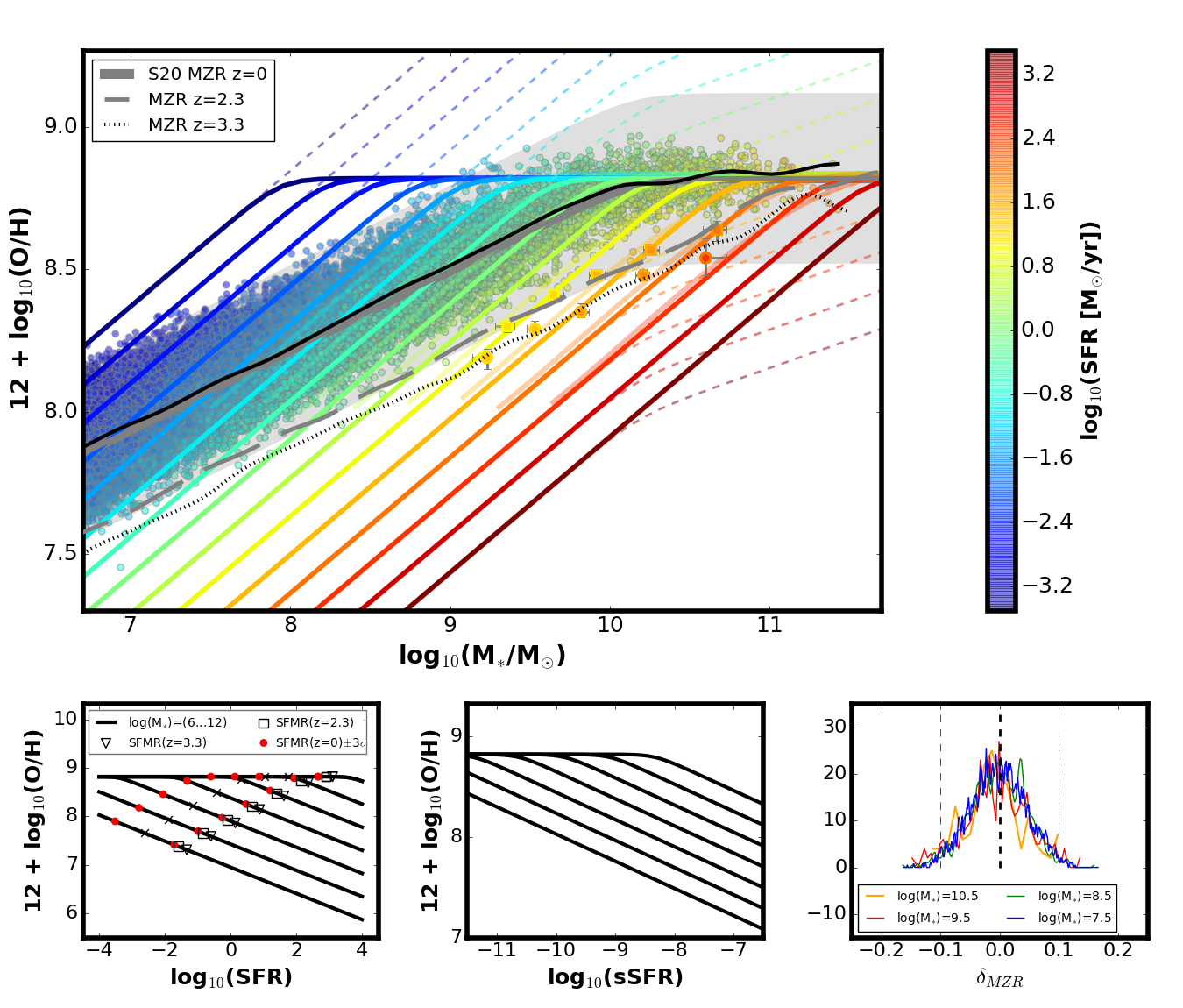
Figure 3: Example $Z_{O/H}(SFR,M_{*})$ obtained with our method (coloured lines - different log₁₀(SFR) values) and using the $z\sim 0$ MZR, SFMR and $\nabla_{\rm FMR0}$ from Sanders et al. (2020) (S20). Colored points are sampled from the GSMF and SFMR at z$\sim$0. Black line is plotted to show that z$\sim$0 MZR (shown as thick solid gray line and shaded area - 3 $\sigma_{\rm MZR}$ region) is well reproduced with our $Z_{O/H}(SFR,M_{*})$ and z$\sim$0 GSMF and SFMR. The gray dashed lines show fits to the maximum density of galaxies sampled from GSMF and SFMR at $z$=2.3 and 3.3 to indicate the projected MZR evolution. Data points are z$\sim$2.3 and 3.3 stacks from S20. Faint lines show FMR fitted by S20. Coloured dashed lines show $Z_{O/H}(SFR,M_{*})$ as would be obtained with eq. 2 and $\nabla_{\rm FMR0}$=0.27 used at all masses and SFRs. Projections onto $Z_{O/H}$-log₁₀(SFR) and $Z_{O/H}$-log₁₀(sSFR) planes are shown in the bottom panels for several log₁₀(M_∗) values (black lines - log₁₀(M_∗) from 6 to 12). In the bottom left panel we indicate the SFR corresponding to SFMR value for a given M_∗ at $z=0$ (cross), 2.3 (square) and 3.3 (triangle). Red dots indicate the SFR of a galaxy $\pm 3\sigma_{SFMR}$ away from the SFMR at $z\sim 0$. The rightmost bottom panel shows the offsets of $z\sim 0$ model galaxies from the $z\sim 0$ MZR, plotted for several mass bins.

In this Section we present an example $Z_{O/H}(SFR,M_{*})$ obtained with our phenomenological model, where we keep all the input assumptions as similar as possible to Sanders et al. (2020). We choose this study, as the authors provide estimates of all the ingredients that are necessary to construct our $Z_{O/H}(SFR,M_{*})$ (the $z\sim 0$ MZR, SFMR and $\nabla_{\rm FMR0}$), which allows for a direct comparison with their results. The resulting $Z_{O/H}(SFR,M_{*})$ is shown in Fig. 3. In the bottom panels we include two other common 2D projection of the FMR: the $Z_{O/H}$-log₁₀(SFR) plane (bottom left panel) and the $Z_{O/H}$-log₁₀(sSFR) plane (bottom middle panel). The thick gray line in the main panel of Fig. 3 shows the $z\sim 0$ MZR as given in Sanders et al. (2020). The coloured points around that line represent the $z\sim 0$ population of star forming galaxies from our model . The black line indicates a fit to the maximum density region occupied by the $z\sim 0$ galaxy sample described above, to ensue that the $z\sim 0$ MZR is reproduced. The right bottom panel shows the $Z_{O/H}$ residuals around the MZR obtained that way for several example log₁₀(M_∗), which shows that the typically indicated intrinsic width of the relation $\sigma_{MZR}\sim$0.1 dex is reasonably reproduced (note that this quantity is not an input in our model). The thick solid coloured lines in the main panel show $Z_{O/H}(SFR,M_{*})$ for various fixed log₁₀(SFR) values. The faint coloured solid lines in the background were obtained with the best-fit FMR given by Sanders et al. (2020) (see eq. 10 therein), plotted roughly in the range of $M_{*}$ and SFR probed by their galaxy sample. We also plot their $z\sim 2.3$ (squares) and $z\sim$3.3 (circles) data points (obtained for stacked spectra of the observed galaxies, see Table 1 therein). The inner (outer) colours in all symbols correspond to upper (lower) bound on the log₁₀(SFR) within the uncertainties provided by the authors for each of the stacks. The long dashed and dotted gray lines indicate the projected $z\sim 2.3$ and $z\sim 3.3$ MZR, calculated in the same way as the black line, but using the $z\sim 2.3$ and $z\sim 3.3$ SFMR from Sanders et al. (2020) respectively, and our GSMF estimated at the corresponding redshifts. The overall agreement is remarkable.
We also show $Z_{O/H}(SFR,M_{*})$ for various fixed log₁₀(SFR) values as would have been obtained with the approach used in Chruslinska & Nelemans (2019) i.e., using eq. 2 with $\nabla_{\rm FMR}$=$\nabla_{\rm FMR0}$=0.27 fixed (i.e. the same at all SFRs and masses, see colored dashed lines in the main panel of Fig. 3). It can be seen that the $Z_{O/H}(SFR,M_{*})$ constructed that way is identical with our model at low/intermediate $M_{*}$ and high SFRs (the strong correlation regime), and starts to deviate at high $M_{*}$ and low SFR (above the $z\sim$0 MZR), where $\nabla_{FMR}<\nabla_{FMR0}$. This demonstrates that the mass and SFR dependence of the SFR-metallicity correlation discussed in Sec. 3.1.5 is present in our description.

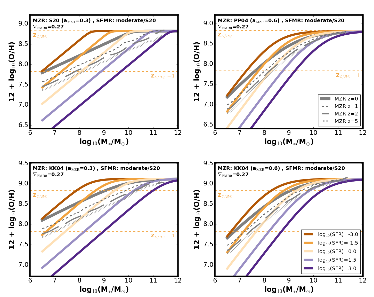
Figure 4: $Z_{O/H}(SFR,M_{*})$ obtained as described in Sec. 3.1 - different colours show $Z_{O/H}(SFR,M_{*})$ at fixed log₁₀(SFR) (increasing from left to right, see legend). Different panels correspond to different choices of the $z\sim 0$ MZR (indicated by the thick gray line). All panels assume SFMR with a moderate flattening ($z\sim 0$ SFMR with a_SFMR=0.72 at high masses and a_SFMR=0.83 at low masses) and $\nabla_{\rm FMR0}$=0.27. Gray dashed lines indicate the projected MZR evolution as obtained by performing fits to maximum density of galaxies in 12+log₁₀(O/H) - log₁₀(M_∗) plane, where the galaxies were sampled from GSMF (assuming $\alpha_{GSMF}$=$\alpha_{fix}$) and SFMR at several higher redshifts and their Z_O/H was assigned using the $Z_{O/H}(SFR,M_{*})$ shown in each of the panels. Horizontal orange lines indicate solar and 10% solar metallicity, assuming Z_O/H⊙=8.83 (Grevesse & Sauval, 1998).

3.4 Model variations

Table 1: Parameters of the different versions of the $z\sim 0$ MZR and SFMR used in this study. The first column gives the name used to reference the variation throughout this study.
^a different SFMR parametrisation (see footnote 9)

	MZR $z\sim 0$
	$a_{\rm MZR}$	log${}_{10}\left(\rm M_{0;MZR0}\right)$	ZO/H;MZR0	$\beta_{MZR}$
PP04	0.6	9.19	8.81	0.6
S20	0.28	10.16	8.82	3.43
KK04a	0.57	9.03	9.12	0.57
KK04b	0.3	9.9	9.12	0.74
	SFRM $z\sim 0$
	$a_{SFMR}$	log${}_{10}\left(\rm M_{0;SFMR0}\right)$	$a_{SFMR2}$	$b_{SFMR}$
no flattening	0.83	-	0.83	-8.241
sharp flatteninga	0.83	9.89	s0=-0.033
moderate/S20	0.83	9.73	0.72	-8.241
moderate/S14	0.83	9.73	0.49	-8.241

In this study we consider several variations of the base $z\sim 0$ MZR and SFMR relations, representing extreme choices of the shapes of the two relations and the MZR normalisation $Z_{O/H;MZR0}$ reported in the literature. We also consider two variations of the GSMF: either with fixed low mass end slope ($\alpha_{GSMF}$=-1.45), or with $\alpha_{GSMF}$ steepening with redshift (see Sec. 3.1. in Chruslinska & Nelemans 2019 for the details).
This allows us to explore the extremes of the f_SFR(Z,z) distribution. We briefly introduce each of the MZR and SFMR variations used to construct our Z_O/H(SFR,M_∗) below.

3.4.1 MZR variations

The MZR is parametrised in the same way as Z_O/H(M_∗,SFR), i.e.:

$$\rm Z_{O/H}(M_{*})=Z_{O/H;MZR0}-\frac{a_{MZR}}{\beta_{MZR}}log\left(1+(\frac{M_{*}}{M_{0;MZR0}})^{-\beta_{MZR}}\right)$$ (7)

MZR parameters for the variations considered in this study are given in the top rows of Table 1.
Variations PP04 and KK04a are identical as in Chruslinska & Nelemans (2019) (where KK04a was labelled KK04) and represent MZR estimates based on the Pettini & Pagel (2004) O3N2 and Kobulnicky & Kewley (2004) metallicity calibrations respectively. Both MZRs have similar slopes $a_{MZR}\sim 0.6$, but differ in normalisation by $\sim$0.3 dex. This difference represents a well known systematic offset between the metallicities derived with the theoretical calibrations (e.g. Kobulnicky & Kewley, 2004) and the so-called direct method or empirical calibrations (e.g. Pettini & Pagel, 2004; Sanders et al., 2020), where the latter yield estimates that are $\sim$2 times lower than the former. The choice of KK04 and PP04 calibrations maximises the difference in $Z_{O/H;MZR0}$ (and in the low/high metallicity tails of the f_SFR(Z,z), see Chruslinska & Nelemans 2019), i.e. metallicity estimates obtained with other methods fall in between (see e.g. Fig 15 in Maiolino & Mannucci, 2019).
Furthermore, we consider two additional variations: S20 and KK04b, that have $Z_{O/H;MZR0}$ as in the PP04 and KK04a variations respectively but a shallower low mass slope $a_{MZR}\sim 0.3$. The S20 variation is based on the recent direct-method based determination from Sanders et al. (2020). The parameters of the KK04b variation were chosen in such a way that the MZR is identical with the one in KK04a variation at log₁₀(M${}_{*}/{\rm~{}M}_{\odot})\gtrsim$8.7 and differs at lower masses (where the original determination was not constrained by the data). Our motivation for including those variations is the following: the shape of the z$\sim$0 MZR, in particular its low mass end slope and log${}_{10}\left(M_{0;MZR0}\right)$ is what sets $\gamma$ and $\rm log_{10}\left(M_{0;SFR}\right)$ within our framework, as the dependence on the SFMR parameters is reduced by multiplication by $\nabla_{FMR}\lesssim 0.3$. However, the MZR slope and turnover mass are not well constrained with the current data (the purely linear regime is often not probed) and depend on the adopted parametrisation, for the same galaxy sample one can fit different a_MZR and turnover masses (e.g. Curti et al., 2020, for the parametrisation used in eq. 1, $\beta$ is also somewhat degenerate with the MZR turnover mass and slope). Recent MZR determinations by Curti et al. (2020) and Sanders et al. (2020) both indicate shallower a${}_{MZR}\sim$0.3 than typically found in earlier studies (a${}_{MZR}\sim$0.6, e.g. Andrews & Martini, 2013; Zahid et al., 2014b). Curti et al. (2020) and Sanders et al. (2020) discuss several potential biases in earlier studies that may be causing this difference (e.g. relatively bright, high SFR galaxies may dominate the low mass end of the sample and therefore induce a bias towards lower metallicity). Alternatively, massive star-based metallicity determination methods (yielding $Z_{O/H;MZR0}$ consistent with empirical/direct methods) lead to a${}_{MZR}\sim$0.6, similar to earlier studies (see discussion in Sanders et al., 2020). Given those differing results and until better observational constraints on the low mass end of the MZR are available, we consider 0.3$\lesssim$a${}_{MZR}\lesssim$0.6 as realistic. Note that this uncertainty in the MZR slope at M${}_{*}\lesssim 10^{8.5}{\rm~{}M}_{\odot}$ leads to significant differences in metallicity when the relation is extrapolated down to low stellar masses (e.g. at log₁₀(M_∗/${\rm~{}M}_{\odot}$)=6 there is $\approx$0.56 dex difference between the metallicity estimated with KK04a and KK04b z$\sim$0 MZR variations and $\approx$0.76 dex difference if S20 and PP04 z$\sim$0 MZR variations are compared). By considering a range of slopes we explore the uncertainty associated with the low mass MZR extrapolation on the (low metallicity part of) f_SFR(Z,z) estimate. In this study, the MZR is only used to construct $Z_{O/H}(SFR,M_{*})$ and we do not need to describe its evolution with redshift.

3.4.2 SFMR variations

To describe the $z\sim 0$ SFMR we follow Chruslinska & Nelemans (2019) and assume the low/intermediate mass slope $a_{SFMR}$ and normalisation $b_{SFMR}$ based on Boogaard et al. (2018). As discussed in Chruslinska & Nelemans (2019), the shape of the high mass end is debated: while many authors report a varying degree of flattening above a certain mass (e.g. Schreiber et al., 2015; Tomczak et al., 2016; Bisigello et al., 2018), others see no evidence for the change of slope (e.g. Renzini & Peng, 2015; Pearson et al., 2018). We consider the same extreme variations as described in Chruslinska & Nelemans (2019): ’no flattening’ - a linear relation between log₁₀(SFR) and log₁₀(M_∗) with a single slope at all masses and ’sharp flattening’ - with a${}_{SFMR}\sim 0$ at high masses (using the parametrisation from Tomczak et al. (2016)). We focus on those two extremes to discuss our results, but use additional ’moderate’ variations in some of the figures introducing our FMR model. Those assume that the slope of the SFMR changes from $a_{SFMR}$ to $a_{SFMR2}<a_{SFMR}$ at log₁₀(M_∗)=log${}_{10}\left(\rm M_{0;SFMR0}\right)$. Variation moderate/S20 assumes a high mass slope as in the $z\sim 0$ SFMR shown in Sanders et al. (2020), while moderate/S14 follows the prescription of Speagle et al. (2014). The relevant parameters for all the SFMR variations are given in the bottom rows of Table 1.
The SFMR evolution with redshift is described as in Chruslinska & Nelemans (2019).

3.4.3 The FMR for the considered model variations

In this section we summarize the key differences between $Z_{O/H}(SFR,M_{*})$ obtained for the different variations of the $z\sim$0 MZR, SFMR and $\nabla_{\rm FMR0}$ considered in this study.
It can be seen from eq. 6 that the impact of the SFMR parameters on the SFR-dependent turnover mass $\rm log_{10}(M_{0;SFR})$ (and on $\alpha$) is reduced by the multiplication by $\nabla_{FMR}\lesssim 0.3$. Considering a range of $a_{SFMR}\sim$0.7-1 spanned by different determinations of the low mass slope of the SFMR present in the literature (see e.g. Fig. 10 in Boogaard et al., 2018) instead of using a fixed value $a_{SFMR}$=0.83 would only affect $\alpha$ by $\lesssim$0.08. This is illustrated by the gray bands in the top panels in Fig. 2. At the same time, for the range of $a_{\rm MZR}$ considered in this study $\alpha$ varies between $\sim$0.2 and 0.55 (compare the orange and blue lines in Fig. 2, where smaller values correspond to steeper MZR slopes). Variation in $\nabla_{\rm FMR}$ between 0.17 and 0.3 affects $\alpha$ by $\sim$0.15 (see green lines and bottom left panel in Fig. 2).
The choice of MZR has a decisive role in setting the $Z_{O/H}(SFR,M_{*})$. $\nabla_{\rm FMR0}$ also visibly affects the relation, while SFMR has a relatively mild impact on its shape within our framework. $Z_{O/H}(SFR,M_{*})$ obtained for the different variations of the $z\sim 0$ MZR considered in this study and for our fiducial $\nabla_{\rm FMR0}$=0.27 is shown in Fig. 4. The shift in normalisation between the PP04/S20 and KK04a/b variations (compare top and bottom panels) as well as the difference in the spacing between the different log₁₀(SFR) lines depending on $a_{\rm MZR}$ (compare right and left panels) are evident. The analogous figures showing the impact of different SFMR (Fig. 18) and $\nabla_{\rm FMR0}$ (Fig. 19) choices are shown in Appendix A. The additional $Z_{O/H}(SFR,M_{*})$ variation with a SFR-dependent $\nabla_{\rm FMR}$ is discussed in Appendix C and illustrated in Fig. 22.
The choice of the SFMR variation (its high mass end) has the strongest effect on the $\beta$ parameter ( see Fig. 17 in the Appendix A, which shows the $\beta$ - log₁₀(SFR) relation for different choices of the local scaling relations). In practice, cases with a SFMR with no flattening/only mild change of slope are well described with a single value of $\beta$. The dependence on SFR becomes apparent in cases with SFMR showing a significant deviation from a single power law. The obtained values of $\beta$ are generally smaller for steeper MZR. $\beta$ is only weakly affected by the choice of $\nabla_{\rm FMR0}$ (shifting towards smaller values with decreasing $\nabla_{\rm FMR0}$). We note that using the $z\sim 0$ MZR from Curti et al. (2020), we can recover their best fit $\beta\sim 2$ (when we assume single power law SFMR).
Before showing the results, we first discuss the treatment of starburst galaxies in our models.

4 Starburst galaxies

A common approach to describe the SFR distribution of galaxies is to use a gaussian distribution centered around the redshift-dependent SFMR . In reality, the SFR of star forming galaxies at fixed stellar mass seems to follow a bimodal, double-gaussian shape. The secondary peak of this distribution is attributed to starburst (SB) galaxies - strong SFMR outliers that feature SFR a few times higher than those of the regular star forming galaxies of the same mass and redshift. Several authors estimate the fraction of starburst galaxies (f_SB; the ratio between the number of galaxies associated with the starburst component of the SFR distribution and the total number of star forming galaxies in the considered mass and redshift range) and report values f${}_{SB}\sim$2-3% (e.g. Rodighiero et al., 2011; Sargent et al., 2012; Béthermin et al., 2012; Ilbert et al., 2015; Schreiber et al., 2015). Despite the relatively low f_SB values, the starburst’s contribution to the total cosmic SFRD could still amount to $\sim 10\%$ at z$\sim$2 due to their high SFR. Boco et al. (2021) use the double gaussian distribution of galaxy SFRs from Sargent et al. (2012) and suggest that accounting for the starburst component can improve the consistency between the cosmic SFRD at z$\gtrsim$2 determined with the use of galaxy stellar mass functions paired with SFMR (as used in Chruslinska & Nelemans, 2019) and that estimated with the use of SFR functions (which better account for the SFR of dusty galaxies at high redshifts; as used in Boco et al. 2019).

Crucially, the above mentioned f_SB determinations are based on galaxy samples limited to relatively massive objects (log₁₀(M_∗/${\rm~{}M}_{\odot}$)$>$10) and $z\lesssim$2. Studies of Caputi et al. (2017) and Bisigello et al. (2018) extend the analysis of the distribution of star forming galaxies in the log₁₀(SFR) - log₁₀(M_∗) plane to much lower masses and higher redshifts. While their results are consistent with the previous determinations at high log₁₀(M_∗), they show that f_SB is a strong function of stellar mass (increasing towards lower log₁₀(M_∗)) and $z$ (increasing with redshift). Moreover, they indicate that starburst galaxies follow a distinct sequence in the log₁₀(SFR) - log₁₀(M_∗) plane that is located $\sim$1 dex above the SFMR. This offset of the starburst sequence relative to SFMR is considerably higher than previously reported (e.g. Sargent et al., 2012; Béthermin et al., 2012). This suggests that the contribution of starburst galaxies to the total SFRD budget can be much higher than previously estimated. If starburst galaxies follow the general FMR (as suggested by the results of Hunt et al. 2012; to our knowledge, there is no evidence to the contrary), they would contribute to the star formation at relatively low metallicities compared to galaxies on the SFMR. Therefore, they affect the low metallicity tail of the f_SFR(Z,z) - crucial for the discussion of the origin of transients as long gamma ray bursts and double black hole mergers. We aim to discuss the possible impact of starbursts on the f_SFR(Z,z) in view of the results reported in Caputi et al. (2017) and Bisigello et al. (2018). In the following section 4.1 we describe the method used to include the contribution of starburst galaxies within our framework.

4.1 Method and considered variations

To account for the contribution of starburst galaxies in our calculations, we follow the procedure outlined below:

• At each redshift, we sample log₁₀(M_∗) of star forming galaxies from the galaxy stellar mass function as described in Chruslinska & Nelemans (2019).

• We use f_SB to describe the fractions of starburst galaxies and regular star forming galaxies at each log₁₀(M_∗) and $z$. Our choice is outlined further in this section.

• The SFR of regular galaxies is given by the SFMR from Chruslinska & Nelemans (2019). The SFR of starburst galaxies at each log₁₀(M_∗) follows a normal distribution with scatter $\sigma_{SB}$. The peak of the distribution can be related to the galaxy’s log₁₀(M_∗) with a linear relation: $\rm log_{10}(SFR_{SB})=a_{SB}log_{10}(M_{*})+b_{SB}$, to which we refer as the starburst sequence We set the value of $b_{SB}$ by defining the offset of the starburst sequence from the SFMR, i.e. $b_{SB}=b_{SFMR}+\Delta_{SB-SFMR}$. The assumed parameters are given further in this section.

• To describe the metallicity at which the starburst galaxies produce stars, we assume that they follow the same FMR as regular star forming galaxies (described in Sec. 3.1).

We consider two sets of parameters describing the properties of starbursts. Firstly, we follow the same implementation as used in the recent study by Boco et al. (2021), which is based on the works of Sargent et al. (2012) and Béthermin et al. (2012). This implementation assumes a constant f_SB=0.03 (independent of mass and redshift), a starburst sequence with scatter $\sigma_{SB}$=0.24, located $\Delta_{SB-SFMR}$=0.59 dex above the SFMR and parallel to the SFMR (specifically, we assume the starburst sequence slope of a_SB=0.83, corresponding to the low mass slope of the SFMR from Chruslinska & Nelemans 2019 ) In light of the results of Caputi et al. (2017) and Bisigello et al. (2018) this implementation severely underestimates both f_SB and the SFR of galaxies on the starburst sequence. Therefore, it likely provides the absolute lower limit on the contribution of starbursts.
Secondly, we follow the results of Caputi et al. (2017) and Bisigello et al. (2018) to model the mass and redshift dependence of f_SB and the properties of the starburst sequence. We provide the details of this implementation in Sec. 4.1.1 and 4.1.2 and refer to it as the B18/C17 implementation in the reminder of this paper.

4.1.1 The fraction of starbursts

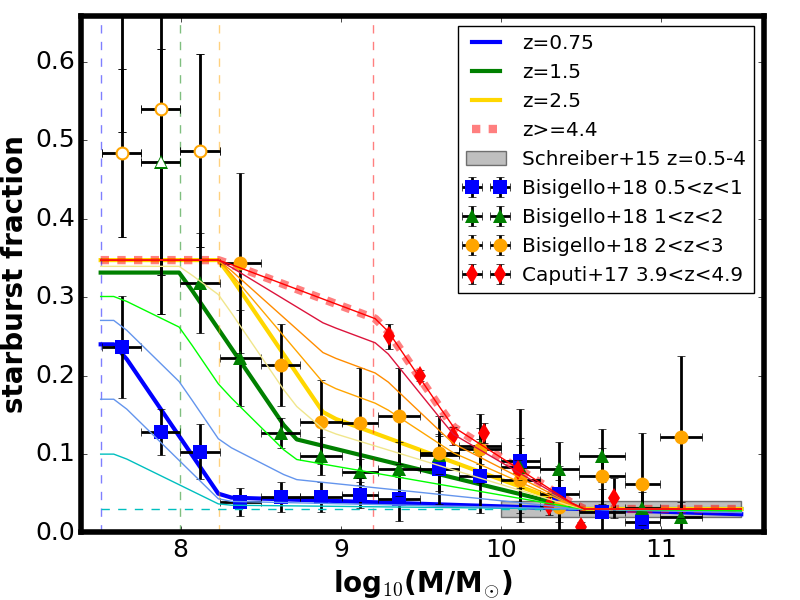
Figure 5: Fraction of starbursts as a function of galaxy stellar mass. Thick lines show the assumed dependence at z$\sim$0.75, 1.5 and 2.5 based on the data from Bisigello et al. (2018) and at z$\sim$4.4 based on Caputi et al. (2017). Thin lines show the interpolation between those redshifts and extrapolation to z=0 (thin horizontal dashed line), plotted with 0.25 step in redshift at z$<$1.5 and with 0.5 step in redshift above. Vertical dashed lines mark log₁₀(M_fix) (see Table. 2) for different redshift bins. Open symbols mark estimates where the galaxy sample from Bisigello et al. (2018) is below 90% mass completeness.

To describe the mass and redshift dependence of $f_{SB}$, we use the observational estimates obtained by Bisigello et al. (2018) (provied for three redshift bins: $0.5<z<1$, $1<z<2$, $2<z<3$; see Fig. 9 therein) and Caputi et al. (2017) ($3.9<z<4.9$, see their Fig. 7). The assumed fraction of starbursts versus stellar mass and redshift is shown in Fig. 5. At each redshift bin covered by the data, we assume the following relation between $f_{SB}$ and log₁₀(M_∗):

$$f_{SB}=\begin{cases}\rm a_{1}log_{10}(M_{*})+b_{1}&\text{if }\rm log_{10}(M_{\rm fix})\leq log_{10}(M_{*})\leq log_{10}(M_{0;SB})\\ \rm a_{2}\ log_{10}(M_{*})+b_{2}&\text{if }\rm log_{10}(M_{0;SB})<log_{10}(M_{*})\leq 10.5\\ \rm\ 0.03&\text{if }\rm log_{10}(M_{*}/{\rm~{}M}_{\odot})>10.5\\ \end{cases}$$ (8)

All stellar masses in eq. 8 are in solar units ${\rm~{}M}_{\odot}$. The adopted coefficients are given in Table 2. We assume that the above relation holds strictly in the middle of each redshift bin and interpolate between them to describe $f_{SB}$ at $0.5<z<4.4$. At z$>$4.4 we use the relation from z=4.4. That way we obtain a conservative estimate of the starburst contribution at higher redshifts. We extrapolate the constructed dependence to lower redshifts, setting a constant starburst fraction of 3% at all masses at z=0.
At z=0.75,1.5 and 2.5, log₁₀(M_fix) is the lower edge of the lowest mass bin where the galaxy sample from Bisigello et al. (2018) is within 90% stellar-mass completeness. We make a conservative assumption and use a fixed $f_{SB}$ value below that mass (i.e., $f_{SB}=\rm a_{1}log_{10}(M_{\rm fix})+b_{1}$). At $z=4.4$, log₁₀(M_fix)=9.25 corresponds to the lowest mass for which the fraction of starbursts has been estimated in Caputi et al. (2017). At this redshift, $f_{SB}$ is fixed at the same mass as at z=2.5 (i.e. log₁₀(M_∗)=8.24) and we assume a linear relation to describe the dependence between log₁₀(M_∗)=8.24 and log₁₀(M_∗)=9.25 . This exception is necessary to avoid a decrease in the fraction of starbursts at log₁₀(M_∗)$<$9.25 at z$>$2.5, which would break the trend seen in the data (see Figure 5). At log₁₀(M_∗)$>$10.5 there is a lot of scatter in the data and the trend is inconclusive. In this mass range we use a fixed value $f_{SB}$=0.03 at all redshifts, as found in earlier studies that focused on the most massive galaxies (e.g. Rodighiero et al., 2011; Schreiber et al., 2015). The steeper, lower mass part of $f_{SB}$ - log₁₀(M_∗) dependence is well described with the same slope across all four redshift bins. Therefore, for simplicity we assume $a_{1}=-0.3$. The slope of the relation in the higher mass part ($a_{2}$) and the mass log₁₀(M_0;SB) separating the high and low mass parts of the relation increase with redshift.

Table 2: Coefficients used in eq. 8, describing f_SB as a function of log₁₀(M_∗) at redshift $z_{bin}$. The remaining coefficient $a_{1}=-0.3$ at all $z_{bin}$

$z_{bin}$	b1	a2	b2	log(M0;SB/${\rm~{}M}_{\odot}$)	log(Mfix/${\rm~{}M}_{\odot}$)
0.75	2.52	-0.0067	0.1	8.25	7.6
1.5	2.73	-0.05	0.555	8.7	7.99
2.5	2.82	-0.075	0.817	8.9	8.24
4.4	3.045	-0.131	1.408	9.7	9.25

4.1.2 The starburst sequence

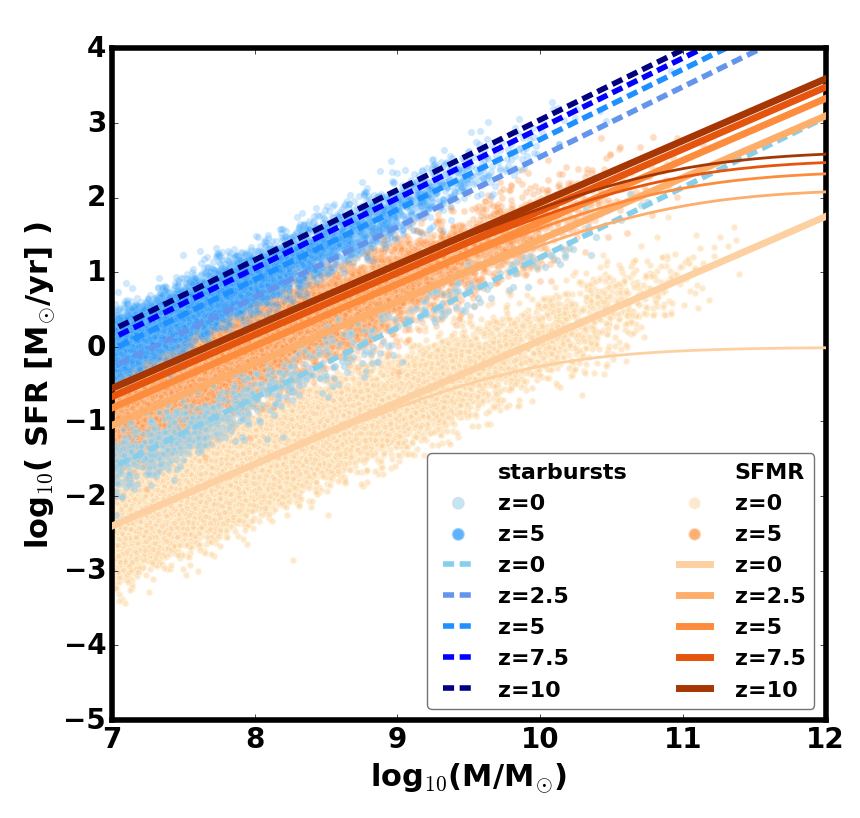
Figure 6: Starburst sequence (SB - dashed lines) compared with the SFMR for extreme assumptions about the high mass slope of the SFMR: no flattening (thick solid lines) and sharp flattening (thin solid lines). Colours correspond to different redshifts. Points sampled from the GSMF and assigned to the SFMR or starburst sequence using starburst fraction shown in Fig. 5 are plotted for z=0 and z=5 to illustrate the increasing fraction of star forming galaxies that populate the starburst sequence at higher redshifts and lower stellar masses. The properties of starbursts are based on the results from Caputi et al. (2017) and Bisigello et al. (2018).

We guide our description of the SFR distribution of starburst galaxies with the results shown in Fig. 3 and Fig. 7 from Caputi et al. (2017) and Fig. 6 and Fig. 7 from Bisigello et al. (2018). The resulting starburst sequence is shown in Fig. 6. The width of the starburst sequence in Caputi et al. (2017) and in Bisigello et al. (2018) is smaller that that of the SFMR, although the values are not given. Guided by the results shown in the figures, we assume $\sigma_{SB}$=0.2 dex. Both Caputi et al. (2017) and Bisigello et al. (2018) find a starburst sequence that is steeper than the SFMR. There is no clear evidence for $a_{SB}$ evolution with redshift. For simplicity, we assume $a_{SB}$=0.94 (average between the best fit values in 3 redshift bins from Bisigello et al. and high redshift estimate from Caputi et al.). To set the offset of the starburst sequence from the SFMR $\Delta_{SB-SFMR}$ we focus on the results for the intermediate masses log₁₀(M${}_{10}/{\rm~{}M}_{\odot}$)$\sim$9-9.5 (where the sample is complete and the SFMR is not affected strongly by the potential flattening at the high mass end). We find that $\Delta_{SB-SFMR}$ in both Bisigello et al. (2018) and Caputi et al. (2017) is about 1 dex and we assume this value in our calculations. Note that the SFMR shown in Caputi et al. (2017) is likely an upper limit on the SFMR location at z$\sim$4.4, which suggests that at those high redshifts the offset might be even larger.

5 Results: the distribution of the cosmic SFRD over metallicities and redshift

In this section we discuss the distributions of the cosmic SFRD over metallicities and redshift (f_SFR(Z,z)) obtained for different variations of our observation-based model (including different choices of the local MZR, SFMR, GSMF, $\nabla_{\rm FMR0}$ and prescriptions to account for starburst galaxies).
Ultimately, we aim to explore the extreme f_SFR(Z,z) cases in terms of the amount of SFRD occurring at low (below 10% solar metallicity; Z${}_{O/H}\leqslant$Z_O/H⊙-1) and high (above solar Z${}_{O/H}\geqslant$Z_O/H⊙) metallicity.
In the remainder of this paper we distinguish between two sets of models based on the choice of the local scaling relations (MZR and SFMR): the ’low metallicity’ f_SFR(Z,z) cases - obtained with $z\sim 0$ MZR with low normalisation (PP04 or S20) and SFMR with sharp flattening at high masses, and the ’high metallicity’ f_SFR(Z,z) cases - obtained with $z\sim 0$ MZR with high normalisation (KK04a or KK04b) and SFMR with no flattening. Other combinations of the local MZR and SFMR lead to more moderate metallicity distributions.

We note that in order to describe the f_SFR(Z,z) at high redshifts and low metallicities (as shown in this Section and needed, for instance, in applications to gravitational wave astrophysics) one needs to extrapolate the FMR well beyond the regions where it is constrained by current observations (in particular to z$\gtrsim$3 and $M_{*}\lesssim 10^{8}{\rm~{}M}_{\odot}$). The importance of the assumed z$\gtrsim$3 extrapolation is discussed in Sec. 5.1, where we compare the f_SFR(Z,z) obtained with the non-evolving FMR and with the redshift-dependent MZR based approach used in Chruslinska & Nelemans (2019). Metallicity of $M_{*}\lesssim 10^{8}{\rm~{}M}_{\odot}$ galaxies assigned with our FMR is primarily sensitive to the MZR slope and normalisation and the strength of the SFR-metallicity anti-correlation at low masses/SFRs. Those factors are discussed in Sec. 5.1.1 and further in Appendix C. In Sec. 5.2 we discuss the f_SFR(Z,z) under different assumptions about the contribution of starburst galaxies.

5.1 f_SFR(Z,z) with redshift-invariant FMR

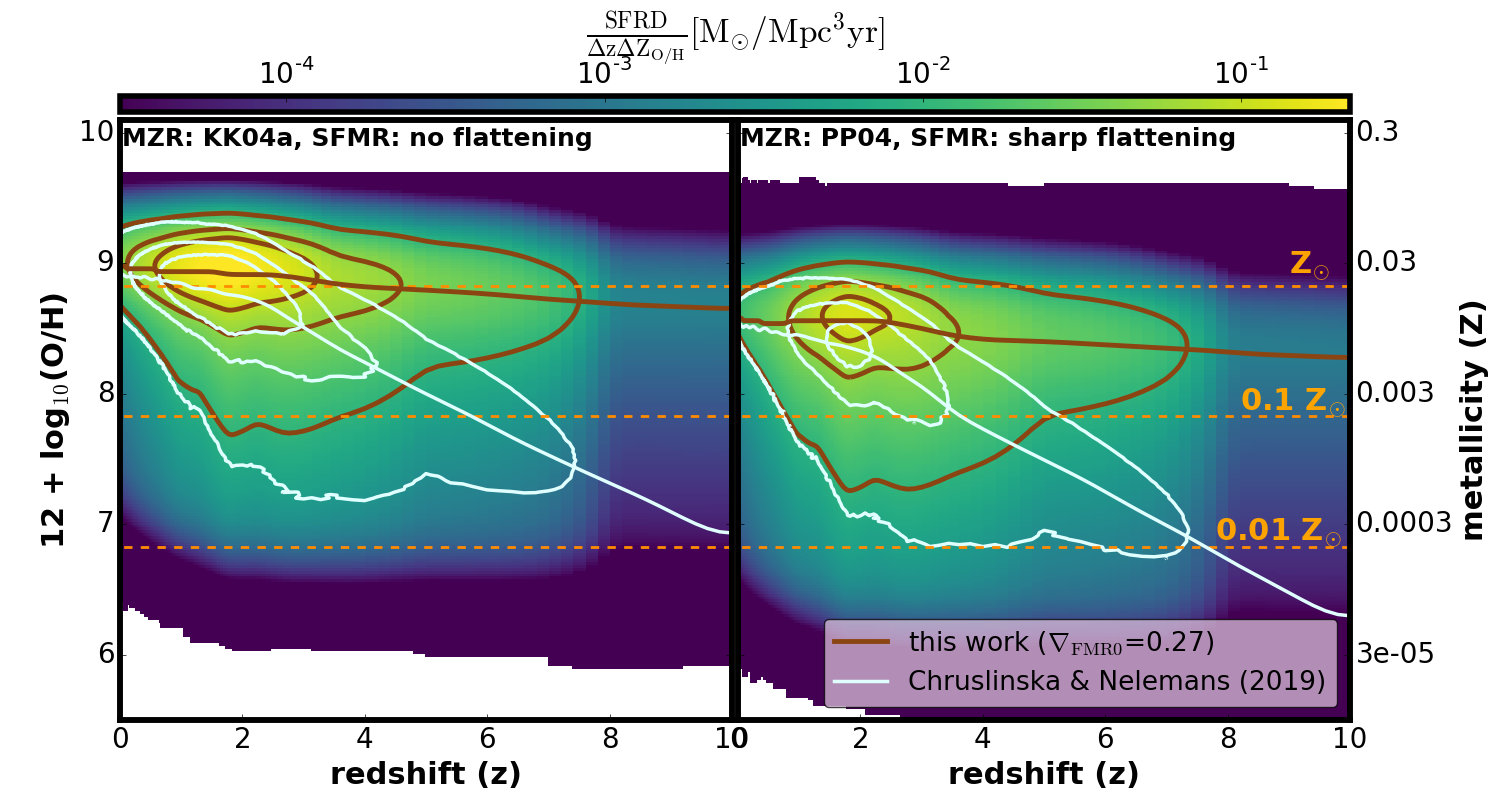
Figure 7: Distribution of the star formation rate density (SFRD) at different metallicities and redshift (z) in this paper (background colours, brown contours; assuming non-evolving FMR and $\nabla_{\rm FMR0}=0.27$) compared to Chruslinska & Nelemans (2019) (white contours, assuming redshift-dependent MZR). Colour indicates the amount of SFRD happening in different redshift and metallicity bins, contours indicate constant SFRD and are plotted for 0.01,0.05 and 0.1 [${\rm~{}M}_{\odot}$/Mpc³yr] (with the highest value corresponding to the most inward contour). Left – model variation with KK04a $z\sim 0$ MZR and SFMR with no flattening at high masses compared with the high metallicity extreme from Chruslinska & Nelemans (2019). Right – model variation with PP04 $z\sim 0$ MZR and SFMR with sharp flattening at high masses compared with the low metallicity extreme from Chruslinska & Nelemans (2019). All models assume GSMF with non-evolving low mass end. Orange horizontal dashed lines indicate solar, 10% solar and 1% solar metallicity (assuming Grevesse & Sauval 1998 solar metallicity scale). The right metallicity axis was obtained from $Z_{O/H}$ assuming solar abundance ratios. Note that beyond z$\gtrsim$3 the distribution relies on extrapolation of the MZR/FMR evolution with redshift - in this respect, the plotted contours contrast somewhat extreme assumptions.

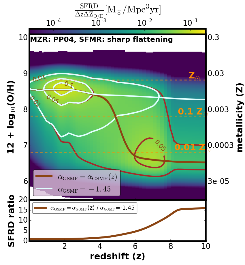
Figure 8: Example illustrating the effect of different assumptions about the low mass end slope of the GSMF ($\alpha_{\rm GSMF}$) on the f_SFR(Z,z). Top panel: brown constant SFRD contours and background colours - variation with $\alpha_{GSMF}$ steepening with redshift (i.e. predicting increasing number density of low mass galaxies), white contours - fixed $\alpha_{\rm GSMF}$=-1.45. Contours are plotted for 0.01,0.05 and 0.1 [${\rm~{}M}_{\odot}$/Mpc³yr]. Both model variations assume $\nabla_{\rm FMR0}$=0.27 and the same SFMR and $z\sim 0$ MZR (indicated in the figure). f_SFR(Z,z) significantly deviate at $z\gtrsim 3$: a redshift-dependent $\alpha_{\rm GSMF}$ leads to most of the SFRD happening at low metallicity and to a higher total SFRD(z). Bottom panel: ratio of the total SFRD at each redshift as obtained in the two variations.

The comparison between the f_SFR(Z,z) constructed with the use of redshift-invariant Z_O/H(SFR,M_∗) and the corresponding distributions from Chruslinska & Nelemans (2019) is shown in Fig. 7. We compare the variations with $z\sim 0$ MZR and SFMR choices as in the high (left) and low (right) metallicity extremes from Chruslinska & Nelemans (2019) (see Sec. 4.2 and Fig. 8 therein). In this section we do not explicitly include starburst galaxies, so that all assumptions that are not related to the metallicity distribution of galaxies are the same as in Chruslinska & Nelemans (2019).

Fig. 7 shows that the metallicity distributions start to deviate around $z\gtrsim$1.5 (compare brown and white contours), where the redshift-dependent MZR predicts a steeper decrease in metallicity than what results from the non-evolving FMR. The difference becomes striking at $z\gtrsim$3, but we stress that neither the MZR nor the FMR is currently constrained in this redshift regime. In particular, there is no guarantee that the FMR holds or continues to show weak/no redshift evolution beyond that redshift. On the other hand, as discussed in Sec. 3, the extrapolated MZR evolution as assumed by Chruslinska & Nelemans (2019) is likely to overestimate the rate of decrease in metallicity. Therefore, in Fig. 7 we contrast two seemingly extreme assumptions. Until better observational constraints are available, this comparison can serve to illustrate (likely a conservative) range of uncertainty of the high redshift part of f_SFR(Z,z) resulting from the extrapolated evolution of the galaxy metallicity distribution with redshift. The extrapolated MZR evolution leads to a $z\sim 10$ peak metallicity that is almost 2 dex lower than what results from the non-evolving FMR assumption. The latter leads to SFRD concentrated at higher metallicities (irrespective of the model variation), but the extended low metallicity tail is still present at all redshifts.
We note that the difference between the f_SFR(Z,z) obtained with a redshift dependent MZR and with the non-evolving FMR was recently discussed in Boco et al. (2021) - qualitatively our results are the same as discussed therein. However, rather than discussing a example f_SFR(Z,z) obtained with a particular FMR or MZR taken from the literature, here we model the FMR consistently with the choice of the local SFMR and MZR and can explore the uncertainties of the final result.
All variations shown in Fig. 7 assume a GSMF with non-evolving low mass slope. As discussed in Chruslinska & Nelemans (2019) (see Sec. 4.1 therein), this assumption has relatively little effect on f_SFR(Z,z) at $z\lesssim$3, but strongly affects the result at higher redshifts (both its low metallicity tail and the total SFRD). This is illustrated in Fig. 8 - the effect of the steepening low mass end of the GSMF on f_SFR(Z,z) is analogous for other model variations.

5.1.1 The effect of the $z\sim 0$ MZR slope and $\nabla_{\rm FMR0}$

The effect of the choice of the $z\sim 0$ MZR slope ($a_{\rm MZR}$) and $\nabla_{\rm FMR0}$ on f_SFR(Z,z) is shown in Fig. 9. Similarly to Fig. 7, the left and right panels show high and low metallicity model variations respectively. Top (bottom) panels show variations with $a_{MZR}\sim$0.3 ($a_{MZR}\sim$0.6). Different contours illustrate the impact of $\nabla_{\rm FMR0}$

As can be expected, f_SFR(Z,z) for variations with steeper $z\sim 0$ MZR (higher $a_{\rm MZR}$ values) have a more extended low metallicity tail at each redshift. However, variations with lower $a_{\rm MZR}$ values feature a much steeper metallicity evolution at $z\lesssim 4$. At higher redshifts the metallicity peak of f_SFR(Z,z) decreases at a similar rate for the variations with the same $\nabla_{\rm FMR0}$ and same total SFRD (i.e. the same SFMR and GSMF assumptions), irrespective of $a_{\rm MZR}$. This can be understood by looking at the comparison of Z_O/H(SFR,M_∗) obtained for different $z\sim 0$ MZR, shown in Fig. 4. In this plane, galaxies with the same log₁₀(M_∗) at higher redshifts shift to higher log₁₀(SFR) lines. The rate of this shifting is dictated by the redshift-dependent SFMR. The offset in Z_O/H between the different log₁₀(SFR) curves at fixed log₁₀(M_∗) is bigger for variations with lower $a_{\rm MZR}$ (compare left and right panels in Fig 4) and similarly for higher $\nabla_{\rm FMR0}$ (see Fig. 19 in the Appendix A). This translates into steeper decrease of the f_SFR(Z,z) metallicity peak with redshift in the variations with lower $a_{\rm MZR}$ and higher $\nabla_{\rm FMR0}$. At sufficiently high redshifts (where almost all galaxies occupy the high SFR, linear regime of Z_O/H(SFR,M_∗)) the spacing in Z_O/H for different log₁₀(SFR) curves is set by the choice of $\nabla_{\rm FMR0}$. Lower $\nabla_{\rm FMR0}$ result in weaker metallicity evolution (compare white and brown contours in Fig. 9). Therefore, for fixed $\nabla_{\rm FMR0}$ and the same assumptions about the SFMR, the rate of metallicity evolution at $z\gtrsim 4$ and fixed log₁₀(M_∗) is essentially the same. However, the full f_SFR(Z,z) distribution is also affected by the GSMF. If the low mass end of the GSMF is allowed to steepen with redshift, the contribution of the low mass (and so - low metallicity) galaxies to the total SFRD at high redshifts is considerably higher than if the low mass end of the GSFM is fixed (see example shown in Fig. 8).
The FMR is not constrained for low mass, low SFR galaxies. Results discussed above assume that those galaxies are well described by the same relation as the galaxies with higher M_∗ and SFR, and that the strength of the SFR-metallicity correlation does not change in this part of the parameter space (i.e. $\nabla_{\rm FMR}$=$\nabla_{\rm FMR0}$). In appendix C we additionally discuss the variation with a SFR-dependent $\nabla_{\rm FMR}$ in which the SFR-metallicity correlation is assumed to disappear (i.e. the FMR breaks down) at SFR corresponding to $z\sim 0$ SFMR galaxies with $M_{*}\lesssim 10^{8}{\rm~{}M}_{\odot}$. Overall, this assumption has minor impact on the estimated f_SFR(Z,z) distribution (see Fig. 23).

Figure 9: Distribution of the star formation rate density (SFRD) at different metallicities and redshift (z) for different assumptions about the $z\sim 0$ MZR slope (top panels: variations with $a_{MZR}\sim$0.3, bottom panels: $a_{MZR}\sim$0.6) and $\nabla_{\rm FMR0}$ (compare different contours; background colours are plotted for variations with $\nabla_{\rm FMR0}$=0.27). Left (right) panels show model variations with $z\sim 0$ MZR and SFMR that maximise the SFRD at high (low) metallicity. Constant SFRD contours are plotted for 0.005,0.01,0.05 and 0.1 [${\rm~{}M}_{\odot}$/Mpc³yr] (the highest value corresponds to the innermost contour). All model variations assume a GSMF with non-evolving low mass end. Variations with flatter $z\sim$0 MZR lead to a more compact metallicity distribution, but their peak decreases with redshift faster than in variations with a steeper $z\sim$0 MZR.

5.2 f_SFR(Z,z): the impact of starbursts

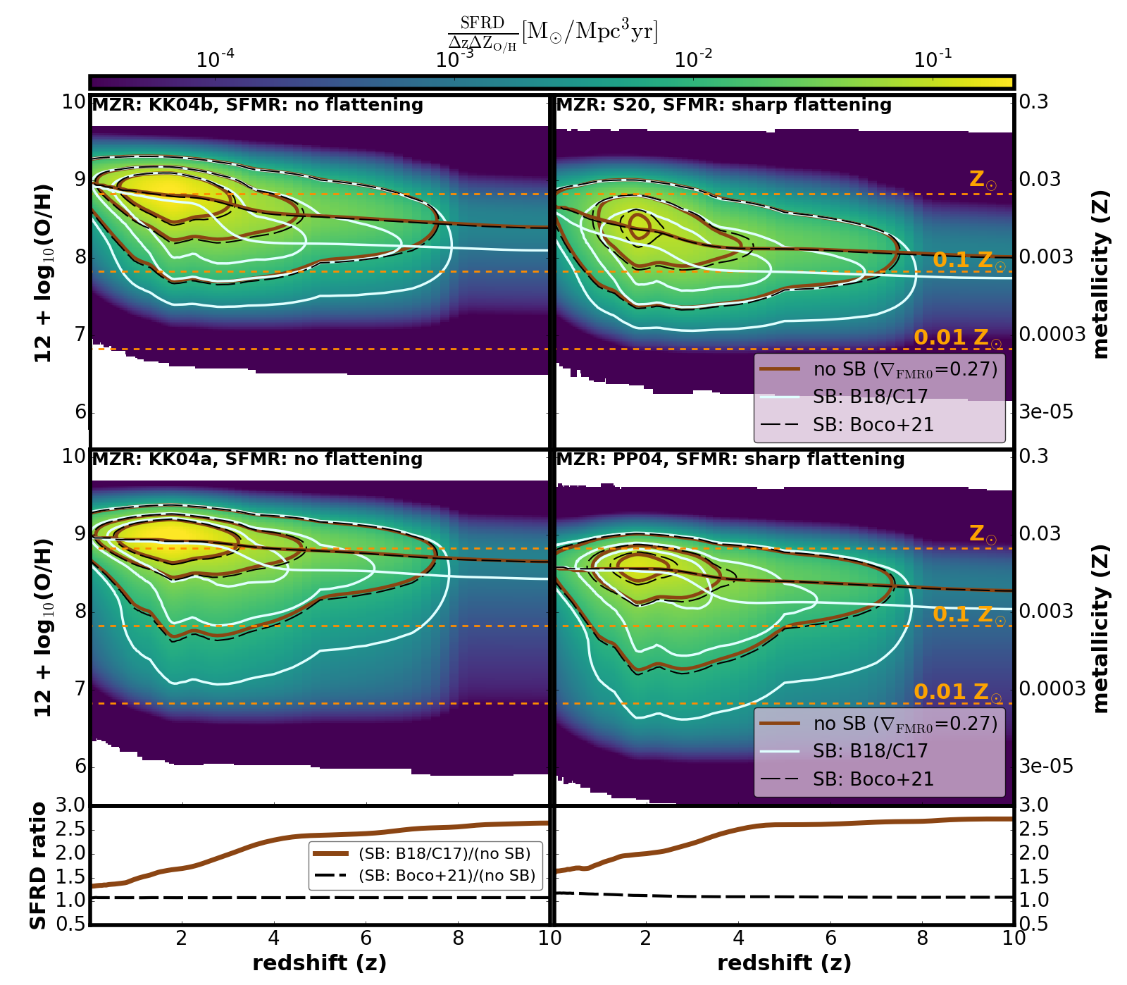
Figure 10: Distribution of the star formation rate density (SFRD) at different metallicities and redshift (z) for different assumptions about starburst galaxies: no starbursts (background colours, brown contours), starburst sequence and f_SB model based on the results of Bisigello et al. (2018) and Caputi et al. (2017) (B18/C17, white contours) and as in Boco et al. (2021) (black dashed contours). Top and middle panels correspond to different $z\sim 0$ MZR and SFMR variations (same as in Fig. 9). Contours indicate constant SFRD and are plotted for 0.01,0.05 and 0.1 [${\rm~{}M}_{\odot}$/Mpc³yr] (with the highest value corresponding to the innermost contour). Note that different assumptions about starburst galaxies lead to different total SFRD at each redshift - bottom panels show the ratio of the SFRD integrated over metallicities at each $z$ in the model with starbursts (brown - B18/C17 implementation, black - Boco et al 2021 implementation) to the corresponding model without starbursts (the choice of MZR does not affect the total SFRD). All models assume GSMF with non-evolving low mass end and $\nabla_{\rm FMR0}$=0.27.

The comparison of f_SFR(Z,z) obtained with and without including starbursts is shown Fig. 10. Top and middle panels show the same $z\sim 0$ MZR and SFMR variations as in Fig. 9. Different contours correspond to different starburst implementations (introduced in Sec. 4.1). The effect of including starbursts in our calculations is twofold: first, a fraction $f_{SB}$ of star forming galaxies is now assigned a higher SFR than what would result from the SFMR. This means that the total SFRD at each redshift is higher than in the model that does not explicitly account for starbursts (see bottom panel in Fig. 10). Second, assuming that starbursts follow the FMR, they contribute to star formation happening at relatively low (for their mass and redshift) metallicity. Therefore, including starbursts shifts the peak of the f_SFR(Z,z) to lower metallicities and broadens the low metallicity part of the distribution.

Both effects are clearly seen when the variations including the B18/C17 starburst implementation (white contours in Fig. 10) are compared with the corresponding variations that do not include starbursts (brown contours). The lower edges of white contours extend to lower metallicities with respect to no starburst case at all redshifts, while the upper, high metallicity edges remain the same. This difference increases with redshift due to increasing f_SB. The total SFRD is about 2.5 times higher at $z\gtrsim$4 in the case with starbursts (brown line, bottom panel in Fig. 10). Note that we fix f_SB beyond $z=4.4$ - the highest redshift bin covered by the data in Caputi et al. (2017). If the trend seen at lower redshift continues, the difference at high redshifts would be even higher.
If instead we follow the starburst implementation as used in the recent study by Boco et al. (2021) (black dashed contours), the difference with respect to cases without starbursts is negligible. This is expected, given the low fixed f_SB=3% and the fact that in this prescription the starburst sequence is within the 2$\sigma_{SFMR}$ scatter of the SFMR. The difference is slightly more pronounced if SFMR with a sharp flattening at high masses is used (right panels in Fig. 10), as in those cases there is a larger difference in SFR between massive galaxies on the SFMR and on the starburst sequence. The inclusion of starbursts as in Boco et al. (2021) also barely affects the total SFRD (see black dashed line in the bottom panel in Fig. 10).

6 Metallicity-dependent cosmic SFH

In this section we discuss the cosmic SFH - SFRD integrated over all metallicities as a function of redshift/cosmic time, as well as the high and low metallicity cuts of the cosmic SFH (i.e. SFRD occurring above and below certain metallicity thresholds) obtained for different model variations. Note that this is essentially a different way to present our results, which provides less detailed information than the full f_SFR(Z,z) distributions shown in Sec. 5. It allows us to zoom into the interesting parts of the distribution and demonstrate the uncertainty of its various parts more clearly. However, we stress that the discussed cuts of the cosmic SFH are sensitive to the considered low/high metallicity thresholds. In some cases, factors that have minor impact on the overall f_SFR(Z,z) distribution may lead to considerable uncertainty in the SFH cut for a particular choice of metallicity threshold. The 10% solar/solar Z_O/H thresholds used here were chosen to zoom into the low/high metallicity tails of the distribution. In general, the relevant thresholds may vary depending on the considered problem.
When showing the cosmic SFH and its various metallicity cuts, in each case we indicate the range of possible outcomes spanned by the model variations with extreme assumptions about the considered factors. We indicate which of the considered factors drives the uncertainty of the f_SFR(Z,z) in different regimes (i.e. low/high metallicity, low/high redshift). As discussed in Sec. 5, the difference between the f_SFR(Z,z) obtained for variations with starburst implementation as in Boco et al. (2021) (i.e. with fixed, small fraction of starbursts) and the corresponding variations with no starbursts is negligible. Therefore, in this section we only discuss the former.

6.1 Cosmic SFH

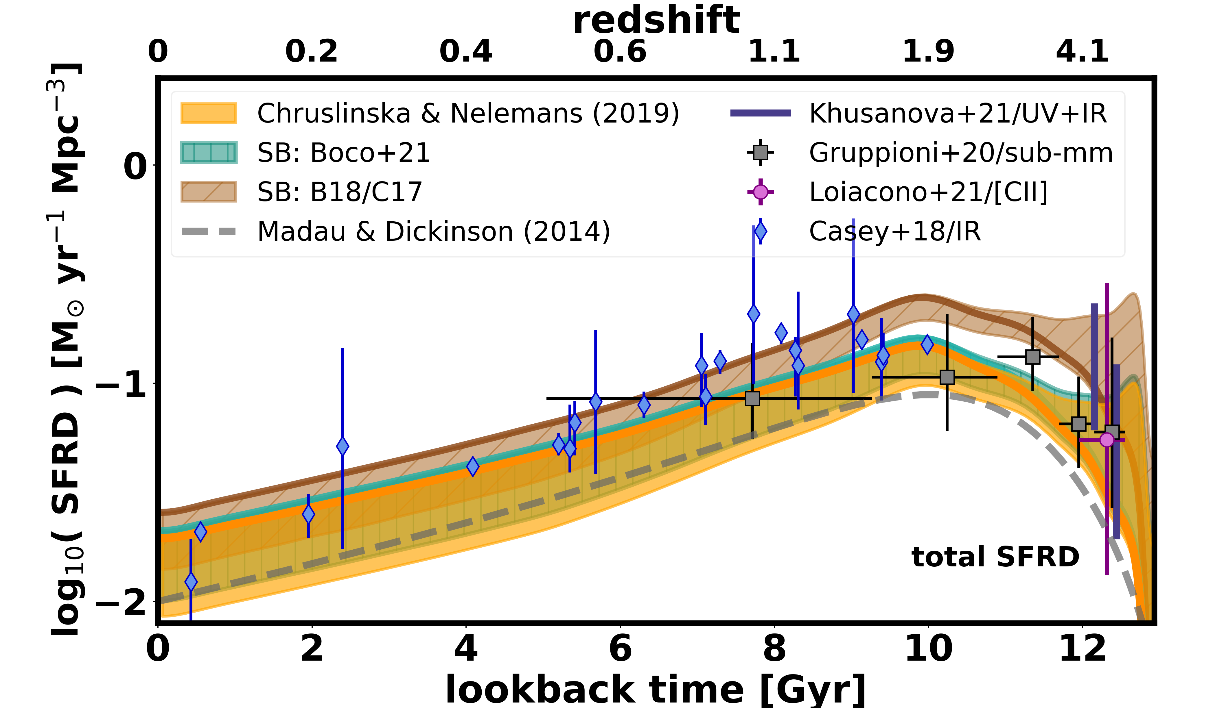
Figure 11: Star formation rate density as a function of lookback time/redshift. The plotted ranges span between the estimates obtained for different variations of model assumptions about the SFMR and GSMF. The ranges in different colours correspond to different assumptions about the starburst galaxies (turquoise: as in Boco et al. (2021), brown: based on Caputi et al. (2017)-C17 and Bisigello et al. (2018)-B18). The orange region shows the corresponding range from Chruslinska & Nelemans (2019) (with no starburst contribution). The thick solid orange and brown lines show how the upper edge of the corresponding range would look like under the assumption of a non-evolving low mass end of the GSMF (the effect on the turquise range follows closely the one that can be seen for Chruslinska & Nelemans 2019, the lower edge is not affected by this assumption). The dashed gray line shows the estimate from Madau & Dickinson (2014) for reference. We overplot the z$\lesssim$2 infrared-based estimates complied by Casey et al. (2018) and the recent observational high redshift SFRD estimates by Loiacono et al. (2021), Khusanova et al. (2021) and Gruppioni et al. (2020), that account for the contribution of heavily dust obscured galaxies. Note that the latter two provide a lower limit. See text for the discussion of the comparison with observations. Where necessary, we correct for the difference in SFR due to varying IMF assumptions.

The cosmic SFH obtained for different model variations considered in this study is shown in Figure 11. Coloured ranges distinguish different assumptions about the starburst galaxies. They span between the extreme cases resulting from different assumptions about the high mass end of the SFMR and the low mass end of the GSMF. Note that the assumptions about the metallicity ($z\sim 0$ MZR, redshift evolution of MZR/non-evolving FMR, $\nabla_{\rm FMR}$) have no impact on the (total) cosmic SFH, but affect its different metallicity cuts. For the convenience of use and discussion, we approximate the results shown in Figure 11 with a broken power law: SFRD = $A$ (1+z)^κ, fitting $A$ and $\kappa$ in several redshift ranges for the upper and lower edge of each variation. The resulting coefficients are given in Table 3. Coefficients obtained when only variations with non-evolving low mass end of the GSMF are considered are provided in Table 4 in the Appendix B.
Considering variations with fixed assumptions about the starburst galaxies, we note the following:

• The uncertainty in the cosmic SFH at z$<$2 is dominated by the assumptions about high mass end of the SFMR: the lower edges of all ranges correspond to variations with SFMR with sharp flattening at high masses (as in low metallicity variations), while the upper edges correspond to variations with SFMR with no flattening (as in high metallicity variations). Assumptions about the GSMF have secondary role in this redshift range.

• The evolution of the low mass end of the GSMF dominates the uncertainty at higher redshifts: the lower (upper) edges of all ranges correspond to variations with non-evolving (steepening) low mass end of the GSMF. At the same time, the importance of the high mass end of the SFMR is reduced due to decreasing number density of the most massive galaxies (see e.g. Fig. 3 in Chruslinska & Nelemans 2019).

• The upper edges of all ranges feature an upturn in the SFRD evolution at $z\gtrsim$4, before the sharp decrease at $z>7$. This is due to strongly increasing number density of low mass galaxies in the variations in which the low mass end of the GSMF steepens with redshift. We note that such upturn only appears when the SFMR and GSMF are extrapolated to log₁₀(M${}_{*})<8$ (see discussion in Chruslinska & Nelemans 2019).

• All variations show a sharp decrease in the SFRD at $z\sim 7$. This is due to the rapid evolution of the GSMF normalisation between $z\sim 7$ and 8, seen when observational GSMF estimates from different redshifts are combined (see Fig. 3 in Chruslinska & Nelemans 2019).

The first three effects are best seen by comparing the thick solid lines in Fig. 11 (corresponding to variations with SFMR with no flattening and GSMF with non-evolving low mass end) with the upper edges of the relevant ranges.
Comparing the variations including starbursts (turquoise/brown ranges) with those from Chruslinska & Nelemans (2019) (that do no explicitly account for their contribution; orange range), one can see that:

• The SFRD is increased in the variations including starbursts; starbursts implementation used in Boco et al. (2021) (turquoise) leads to negligible difference, while the B18/C17 implementation (brown) leads to a factor of $\sim$2.5 increase at high redshifts (see Sec. 5.2)

• variations including starbursts span a narrower range in cosmic SFH (the lower edge is lifted with respect to no starbursts case). This is due to the fact that assigning high SFR (compared to SFMR values) to a fraction of galaxies (starbursts) effectively reduces the difference between the SFRD in model variations with no/sharp SFMR flattening. The effect is stronger at high redshifts for the B18/C17 prescription, as f_SB increases with redshift.

• the increasing fraction of starbursts in the B18/C17 variations leads to a broader peak of the cosmic SFH and a shallower SFRD decrease at high redshifts.

In Figure 11 we contrast the total SFRD that results from various realisations of our observation-based model with several observational determinations of this quantity. At z$<$2, there is about a factor of 2 (2.5) offset between the SFRD obtained with model variations that assume SFMR with no flattening at high masses (and C17/B18 starburst implementation) and the commonly used, best-fit estimate from Madau & Dickinson (2014) (gray dashed line). However, we note that this offset is within the scatter and uncertainty of the z$\lesssim$2 observational estimates - in particular, infrared based SFRD determinations suggest higher SFRD than the estimate obtained by Madau & Dickinson (2014), more in agreement with our SFRD determination based on the GSMF, SFMR, and starburst sequence (see also Fig. 1 in Casey et al. 2018 - the infrared-based data complied by those authors are also included in Fig. 11; and Fig. 2 and discussion in Boco et al. 2021).
At higher redshifts ($2<z<7$), our model variations (even those not including starbursts) in general show shallower SFRD decrease than the estimate provided by Madau & Dickinson (2014) (SFRD$\propto(1+z)^{-2.9}$). This is striking for the upper edges of our estimates (see also Tab. 3). Shallower SFRD evolution than estimated by Madau & Dickinson (2014) is in line with the most recent high redshift observational estimates (e.g. Khusanova et al., 2021; Gruppioni et al., 2020; Loiacono et al., 2021, although the uncertainties in those measurements are still substantial), indicating that a significant fraction of the SFRD at $z\gtrsim 2$ still occurs in dust obscured galaxies (and hence was missed by the earlier - mostly UV light-based surveys). Those estimates are also included in Fig. 11.
However, the comparison of our results with those estimates is not straightforward for two main reasons: a) observations may be incomplete: the estimate provided by Khusanova et al. (2021) is based on a UV selected sample and may not fully account for extremely dusty galaxies, while the estimate provided by Gruppioni et al. (2020) does not account for the contribution of UV sources b) the faint (low mass) end of the galaxy population is not directly probed by observations. All estimates shown in Fig. 11 include (different) extrapolations to account for their contribution to the total SFRD. In our models we extrapolate all of the empirical relations down to log₁₀(M${}_{*}/{\rm~{}M}_{\odot})=6$ - as discussed above, the result of this extrapolation at high $z$ is very sensitive to the GSMF slope. Extrapolations used in the high redshift observational estimates give less weight to low-mass galaxies than our models with steepening low mass end of the GSMF. The estimate by Khusanova et al. (2021) includes extrapolations down to M_∗/luminosity limit comparable to the extrapolation limit used in our study, but is averaged over the results obtained with different GSMF/UV luminosity functions (with different low mass end slopes) from the literature. Gruppioni et al. (2020) extrapolate the infrared luminosity function down to low luminosities. However, such galaxies are expected to be relatively unobscured and the faint-end slope of the infrared luminosity function is much flatter than that of the UV luminosity function (and the GSMF used in our study) at high redshifts - in that sense, this estimate underestimates the contribution of low mass galaxies to the total SFRD. Therefore, the observational estimates are likely lower limits when compared to our models.
We note that all model variations with fixed low mass end of the GSMF and no/small fraction of starbursts fall below the recent $z\sim 3$ limit from Gruppioni et al. (2020). Given the fact that this determination underestimates the contribution of low mass galaxies to the total SFRD with respect to our models, this offset may hint at the need for higher contribution of massive galaxies than included in those model variations (e.g. higher fraction of starburst galaxies or higher overall normalisation of the SFMR at those redshifts). We also note that the z$\sim$4.5 estimate by Khusanova et al. (2021) falls above our estimates obtained with fixed low mass end of the GSMF and no/small fraction of starbursts, but it is unclear how to properly compare this averaged estimate with our results. All model variations are consistent with the limits obtained by Gruppioni et al. (2020) and Loiacono et al. (2021) (although the latter is not particularly constraining due to large uncertainty that overlaps with all of the considered model variations) at similar redshifts.

Table 3: Coefficients of the power law fits to the cosmic SFH (lower and upper edges of the ranges shown in Fig. 11) obtained for different variations of our observation-based model. Within each redshift range indicated in the first column total SFRD can be approximated with the dependence: SFRD=A$\cdot(1+z)^{\kappa}[{\rm~{}M}_{\odot}/yr]$. Note that the cosmic SFH in ’no SB’ variation is identical with the cosmic SFH from Chruslinska & Nelemans (2019).

cosmic SFH - lower edge
variation:	no SB		SB: Boco+21		SB: B18/C17
$z$ range	$\kappa$	A	$\kappa$	A	$\kappa$	A
0$<z\leqslant$1	2.6546	0.0076	2.6093	0.0091	2.7828	0.0123
1$<z\leqslant$1.8	2.4050	0.0091	2.3416	0.0109	2.7119	0.0129
1.8$<z\leqslant$3	-1.0535	0.3195	-1.1284	0.3891	-0.7558	0.4585
3$<z\leqslant$7	-2.2771	1.7427	-2.2909	1.9499	-1.9628	2.4435
7$<z\leqslant$8.8	-12.5425	3.249$\cdot 10^{9}$	-12.5526	3.607$\cdot 10^{9}$	-12.4895	7.845$\cdot 10^{9}$
8.8$<z\leqslant$10.	0	0.0012	0	0.0013	0	0.0033
cosmic SFH - upper edge
variation	no SB		SB: Boco+21		SB: B18/C17
$z$ range	$\kappa$	A	$\kappa$	A	$\kappa$	A
0$<z\leqslant$1	2.2214	0.0194	2.2222	0.0209	2.3850	0.0248
1$<z\leqslant$1.8	1.8708	0.0247	1.8708	0.0266	2.2515	0.0272
1.8$<z\leqslant$4	-1.2436	0.6097	-1.2445	0.6585	-0.5342	0.4793
4$<z\leqslant$7	0.6591	0.0285	0.6585	0.0307	0.7477	0.0609
7$<z\leqslant$8.8	-9.3760	3.29$\cdot 10^{7}$	-9.3864	3.624$\cdot 10^{7}$	-9.4740	1.037$\cdot 10^{8}$
8.8$<z\leqslant$10.	0	0.0168	0	0.018	0	0.0421

6.2 A low metallicity cut of the cosmic SFH

6.2.1 Note on the low metallicity threshold

When referring to low metallicity, throughout this paper we use a limit of $<$10% solar oxygen abundance (with $Z_{O/H\odot}$ following Grevesse & Sauval 1998) and the numbers quoted later in this Section necessarily depend on this choice. This threshold is chosen arbitrarily and serves for illustrative purposes. In general, the relevant definition of low metallicity varies depending on the discussed problem and application. For instance, the abrupt drop commonly seen in the metallicity dependence of the formation efficiency of black hole - black hole mergers formed in the course of isolated binary evolution appears at metallicities 10% - 50% solar (depending on the considered model of binary/stellar evolution, e.g. Chruslinska et al. 2019, Broekgaarden et al. (2021) in prep.). In that sense, depending on the model, the interesting low metallicity threshold could be as high as 50% solar metallicity. Furthermore, from the point of view of evolution of massive stars and the related transients, the most relevant metallicity tracer is iron rather than oxygen (which serves as a metallicity proxy in this study; the oxygen abundance is the most easily obtained from emission line measurements and so it is the most commonly used metallicity proxy in studies of interstellar medium of galaxies). That is primarily due to high sensitivity of the radiation-driven mass loss rates of hot, massive stars to the abundance of this element (e.g. Vink et al., 2001; Vink & de Koter, 2005; Gräfener & Hamann, 2008; Sanders et al., 2020). In general, interstellar medium (ISM) of galaxies is enriched in oxygen and iron on different timescales due to the fact that different sources dominate the production of those elements (core-collapse supernovae with $\lesssim$10 Myr delay with respect to star formation for oxygen and SNIa supernovae with $\sim$0.1-1 Gyr delay for iron; e.g. Wheeler et al. 1989). This means that especially young, highly star-forming galaxies (i.e. typical at high redshifts) are expected to show overabundance of oxygen relative to iron with respect to solar ratios. Recent studies indeed find evidence for super-solar O/Fe$\gtrsim$2 (O/Fe)$|_{\odot}$ in the ISM of $z\sim 2$ star forming galaxies (e.g. Steidel et al., 2016; Topping et al., 2020; Cullen et al., 2021). Consequently, oxygen (or, more generally, $\alpha$-element)-enhanced abundance ratios are also found in local stars that formed at earlier cosmic epochs (e.g. Bensby et al., 2004; Tolstoy et al., 2009). There is no universal way to translate metallicity measure based on oxygen abundance to iron abundance, in particular the typical oxygen to iron ratio in the ISM (and the interesting low metallicity threshold - if oxygen is used as a proxy) can be expected to vary with redshift and possibly galaxy characteristics. A more thorough discussion of this issue is beyond the scope of this work and is left to future studies.

6.2.2 Results

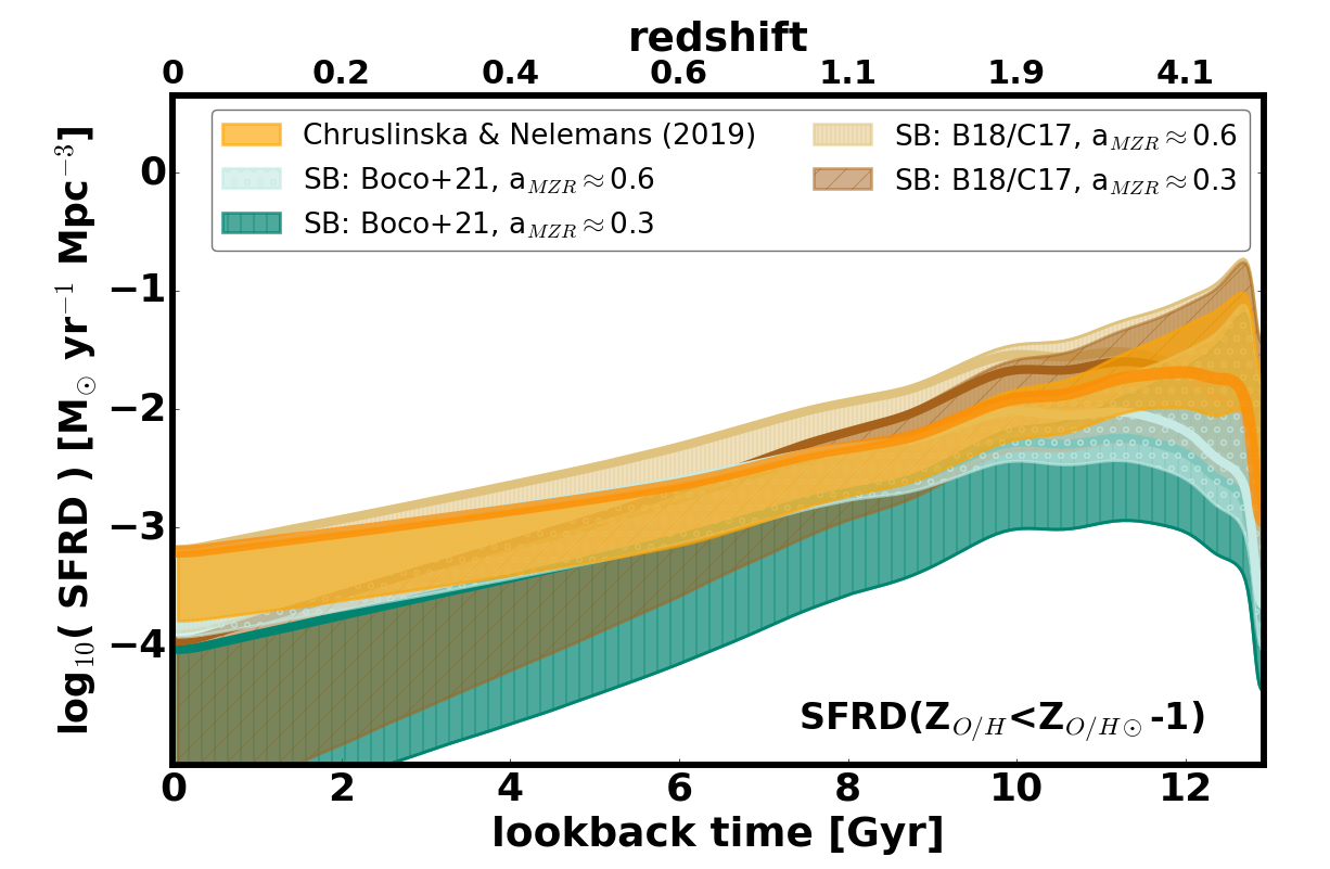
Figure 12: Star formation rate density at low metallicity (i.e. below 10% solar, assuming solar oxygen abundance Z_O/H⊙=8.83 Grevesse & Sauval (1998)) as a function of lookback time/redshift. The plotted ranges show estimates obtained for different variations of assumptions about the starburst (SB) galaxies (blue/turquoise: as in Boco et al. (2021), brown/beige: based on Caputi et al. (2017)-C17 and Bisigello et al. (2018)-B18) and low mass slope of the redshift $z\sim 0$ MZR ($a_{\rm MZR}$). The orange region shows the range of the low metallicity SFHs obtained by Chruslinska & Nelemans (2019). Thick solid lines in different colours indicate the location of the upper edge of the corresponding ranges obtained with the assumption of non-evolving low mass end of the GSMF, demonstrating the importance of this assumption beyond the peak of the cosmic SFH. All variations from this study assume $\nabla_{\rm FMR0}=0.27$.

SFRD that occurs at Z${}_{O/H}<$Z_O/H⊙-1 as a function of redshift/time for different variations of our model is shown in Figure 12. Note that the assumptions about the high mass end of the SFMR have no impact on the low metallicity tail of f_SFR(Z,z) and the low metallicity SFH. Similarly as for the cosmic SFH, we provide the power law fits to the upper and lower edges of the ranges shown in Figure 12 fitted in several $z$ ranges. Those are listed in Tab. 6 and Tab. 5 in the Appendix B. The following features are common to all model variations:

• At $z\lesssim 2$ the SFRD occurring at low metallicity increases faster than the total SFRD. The exact slope depends on the variation. In this redshift range the width of the ranges is set by the assumptions about the $z\sim 0$ MZR: lower/upper edges of all ranges correspond to variations with high/low MZR normalisation (as in the high/low metallicity variations). At those redshifts, assumptions about the low mass end of the GSMF have negligible impact on the amount of star formation happening at low metallicity.

• Beyond the peak of the cosmic SFH assumptions about the low mass end of the GSMF set the width of the ranges and the behaviour of the upper edges. The lower/upper edges correspond to variations with high/low MZR normalisation and non-evolving/steepening GSMF low mass end.

• If $\alpha_{GSMF}$ is fixed, the low metallicity cut of the SFH shows a broad peak between z=2-4 (depending on the variation) and a relatively mild evolution up to z$\sim$7.

• If $\alpha_{GSMF}$ evolves with redshift, the increasing abundance of low mass galaxies (forming stars at low metallicity) causes a continuous increase in the low metallicity cut of the SFH up to z$\sim$7.5-8.

• All variations show a sharp decrease in the low metallicity SFRD at z$\gtrsim$8, reflecting the sharp drop in the total SFRD at those redshifts.

The impact of the assumed $z\sim 0$ MZR slope can be seen by comparing pale blue and turquoise or beige and brown ranges in Figure 12. At low redshifts, variations with steeper MZR slope lead to $\sim$10 times higher SFRD at low metallicity. This is due to the presence of a more extended low metallicity tail of the f_SFR(Z,z) (see Sec. 5.1.1). Lower $a_{\rm MZR}$ lead to more compact f_SFR(Z,z) - in those cases, for the high metallicity variations even the low mass galaxies contribute to SFRD at Z_O/H above the considered threshold of 10% solar metallicity. This difference is reduced at higher redshifts due to steeper metallicity evolution of variations with lower $a_{\rm MZR}$ values - the slope of the low metallicity SFH redshift dependence at $z\lesssim 2$ depends on the $z\sim 0$ $a_{\rm MZR}$.
The slope of the dependence is also affected by the contribution of starbursts (compare pale blue and beige or turquoise and brown ranges). As expected, if the fraction of starbursts increases with redshift (B18/C17 implementation), the low metallicity cut of the SFH increases faster towards high redshifts. At $z\lesssim$0.2 (within the last $\sim$2 Gyr) there is little difference in the amount of SFRD occurring at low metallicity between the variations with no/low fraction of starbursts and the B18/C17 implementation. The contribution of starbursts only becomes evident at higher redshifts. At the peak of the cosmic SFH variations with the B18/C17 starbursts implementation lead to $\gtrsim$3 times higher SFRD at Z${}_{O/H}<$Z_O/H⊙-1 than the corresponding variations with no/low fraction of starbursts
As discussed above, at $z\gtrsim 2$ the slope of the redshift dependence of the low metallicity SFRD and the location of the peak of this dependence is dominated by the assumptions about $\alpha_{GSMF}$. Observational tracers of star formation happening at low metallicity available at high redshifts (e.g. the volumetric rate of long gamma ray bursts or, potentially, that of black hole – black hole mergers as a function of redshift) could help to discriminate between the different variations of our models. In particular, it could provide information about the contribution of low mass galaxies to the total SFRD at high redshifts (thereby constraining jointly the low mass SFMR and GSMF) - difficult to constrain with regular galaxy surveys.

Considering all model variations discussed in this section, the overall spread between the estimates of the SFRD happening below Z${}_{O/H}<$Z_O/H⊙-1 ranges between $\sim$1.6 dex around the peak of the cosmic SFH and $\sim$3 dex at $z>$8. At $z\sim$0 there is $\sim$2.3 dex variation between the different estimates. The uncertainty is dominated by the assumptions about $a_{\rm MZR}$. At the peak of the cosmic SFH the spread is somewhat reduced due to steeper metallicity evolution in variations with lower $a_{\rm MZR}$. At $z\sim$8 the spread increases to $\sim$2.5 dex if the low mass end of the GSMF is allowed to steepen with redshift, and remains close to $\sim$1.6 dex if only variations with fixed $\alpha_{\rm GSMF}$ are considered.
Note that the overall spread between the low metallicity SFH estimates discussed in this study is significantly larger than $\sim$0.5-1.2 dex found in Chruslinska & Nelemans (2019) for the same low metallicity threshold. In their study, effectively only the variations due to the uncertain MZR normalisation and the redshift evolution of the low mass end of the GSMF (which are also included in our analysis) were explored. This difference highlights the importance of the additional factors discussed in this study for the low metallicity cut of the cosmic SFH.
Note that the spread in the low metallicity SFH estimates as discussed above is not only due to differences in the metallicity distribution of the SFRD at different redshifts found for the considered model variations, but also due to their different total SFRD. The latter differences are effectively eliminated in Fig. 20 in Appendix B, where we additionally show the fraction of the total SFRD that happens at $Z_{O/H}<Z_{O/H\odot}$-1 as a function of redshift for the discussed model variations.

Finally, we note that the low metallicity part of the SFH is very sensitive to the adopted log₁₀(M_∗) limit down to which all the empirical relations are extrapolated. This is especially important at $z\lesssim$1, where the low metallicity star formation is limited to low mass galaxies, and at z$\gtrsim$4, due to the potential steepening of the low mass end of the GSMF. With the current data there is no guarantee that those relations can be safely extrapolated to galaxy masses below log₁₀(M${}_{*}/{\rm~{}M}_{\odot}$)$\lesssim$8. However, given their abundance, completely neglecting the contribution of those galaxies is not a satisfactory solution either. In variations favoring high metallicity (i.e. with high MZR normalisation, shallow MZR slope, no/low contribution of starburst galaxies) ignoring the contribution of galaxies with log₁₀(M${}_{*}/{\rm~{}M}_{\odot}$)$<$8 would lead to negligible amount of SFRD happening below 10% solar metallicity even beyond the peak of the cosmic SFH. If the SFR-metallicity correlation significantly weakens/disappears at low specific SFR (see additional model variation discussed in Appendix C and Fig. 25), this may also significantly reduce the estimated amount of SFRD happening below 10% solar metallicity in variations with relatively flat MZR. In those cases, the low/intermediate redshift star formation can only take place below 10% solar metallicity in low mass galaxies that are MZR outliers (see e.g. left bottom panel in Fig. 4 and in Fig. 22), and so the result strongly depends on the adopted FMR extrapolation. Until better constraints on the properties of the low mass end the star forming galaxy population are available, those extrapolations are important source of uncertainty for both the total cosmic SFH, as well as for its low metallicity cut.

6.3 A high metallicity cut of the cosmic SFH

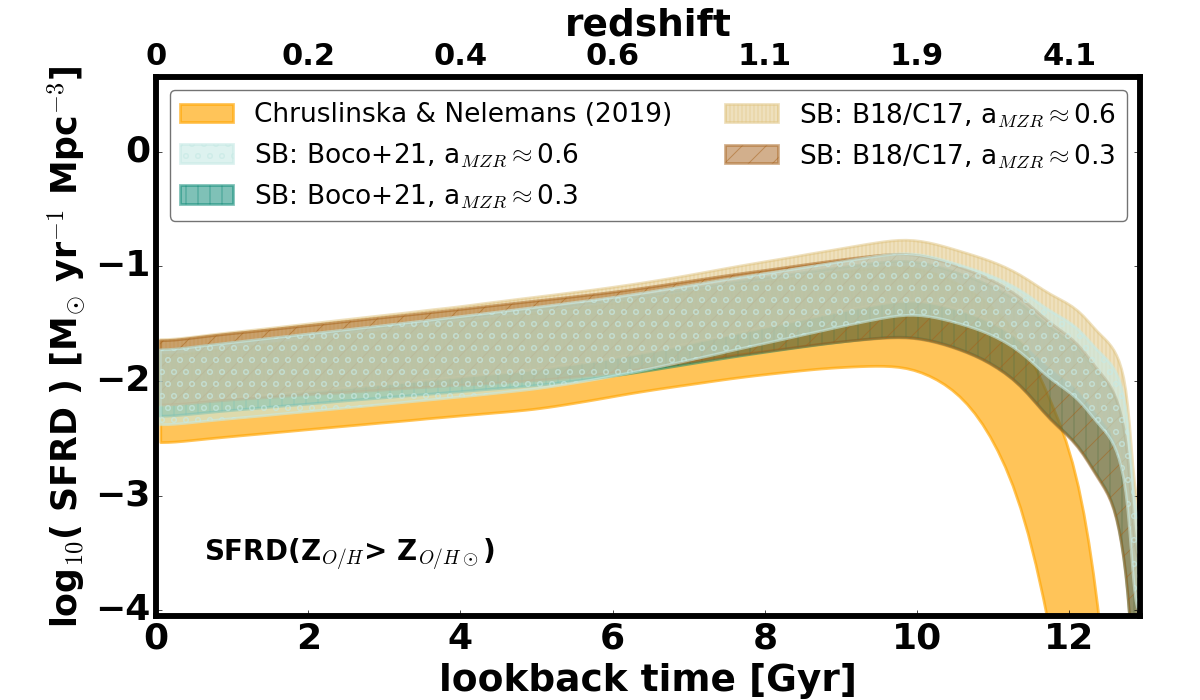
Figure 13: Star formation rate density at high metallicity (above solar, assuming Z_O/H⊙=8.83 Grevesse & Sauval (1998)) as a function of lookback time/redshift. The plotted ranges show estimates obtained for different variations of assumptions about the starburst galaxies (blue/turquoise: as in Boco et al. (2021), brown/beige: based on Caputi et al. (2017)-C17 and Bisigello et al. (2018)-B18) and low mass slope of the redshift $z\sim 0$ MZR ($a_{\rm MZR}$). The ranges span between the low and high metallicity extremes as defined in the text and assume $\nabla_{\rm FMR0}=0.27$. The orange region shows the corresponding range from Chruslinska & Nelemans (2019). Note that starburst galaxies contribute to SFRD at relatively low metallicity and have little impact on the high metallicity cut of the SFRD.

The high metallicity cut of the cosmic SFH - i.e. SFRD that occurs at Z${}_{O/H}>$Z_O/H⊙ as a function of redshift/time for different variations of our model is shown in Fig. 13. This quantity is relatively well constrained in our models when compared to the low metallicity cut of the SFH discussed in the previous section: the overall spread between the estimates obtained with different model variations from this study ranges from $\sim$0.8 dex at $z\sim 0$ to $\sim$1.8 dex at $z\gtrsim$7. The biggest difference appears between the estimate from Chruslinska & Nelemans 2019 (orange range) and all the variations from this study, which lead to considerably higher SFRD occurring at high metallicity beyond the peak of the cosmic SFH. As discussed in Sec. 5.1, this is due to the fact that the non-evolving FMR assumption leads to much slower metallicity evolution when compared to that implied by the extrapolated redshift dependent MZR. The general features that can be seen for all ranges shown in Fig. 13 can be summarised as follows:

• The high metallicity cut of the SFH shows a gradual increase towards the peak of the SFH ($z\sim 2$) and a sharp decrease at high redshifts. This reflects the evolution of the total SFRD. However, the increase towards the peak is shallower and the later decrease is sharper - both due to the overall shifting of the SFRD towards lower metallicities at earler epochs.

• The width of the ranges is set by the assumptions about the SFMR and $z\sim 0$ MZR: upper edges of all ranges correspond to high metallicity variations, lower edges of all ranges correspond to low metallicity variations. Assumptions about the low mass end of the GSMF have negligible effect on the high metallicity cut of the cosmic SFH.

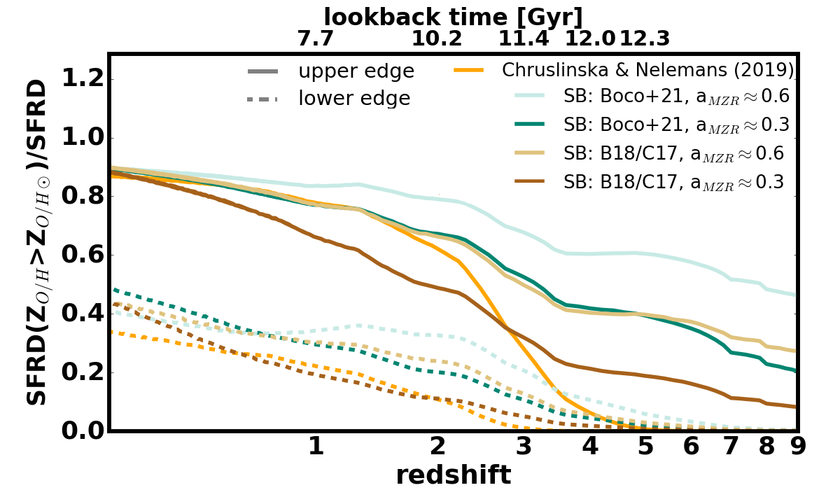
Figure 21: Fraction of the total SFRD that occurs above Z_O/H⊙ as a function of redshift/lookback time, plotted for the model variations shown in Fig. 13. Different colours correspond to different assumptions about $a_{MZR}$ and starburst galaxies (see legend). Thick solid (dashed) lines mark the upper (lower) edges of the corresponding ranges for each of the model variations.

Comparing the ranges obtained for different assumptions about the MZR slope (brown and beige or pale blue and turquoise), one can see that the results start to deviate at $z\gtrsim 1$, where variations with steeper MZR lead to higher SFRD at high metallicity. This is due to slower evolution of the metallicity distribution at $z\lesssim 4$ for those variations, as discussed in Sec. 5.1.1. Assumptions about starbursts have little effect on the Z${}_{O/H}>$Z_O/H⊙ metallicity cut of the cosmic SFH (compare light blue/turquoise and beige/brown ranges). This is due to the fact that (given the FMR), those galaxies only contribute to star formation at relatively low metallicities.
The fraction of the total SFRD that happens at $Z_{O/H}>Z_{O/H\odot}$ as a function of redshift for the discussed model variations is shown in Fig. 21 in Appendix B.

6.4 The impact of $\nabla_{\rm FMR0}$ on the low/high metallicity cut of the cosmic SFH

Figure 14: Example illustrating the effect of $\nabla_{\rm FMR0}$ on the high metallicity cut of the cosmic SFH. The plotted range shows estimate obtained with B18/C17 starbursts implementation and $a_{\rm MZR}\sim$0.3, assuming $\nabla_{\rm FMR0}$=0.27 (same as in Fig. 13). Gray solid (black dashed) lines mark the location of the upper and lower edges of that range obtained with $\nabla_{\rm FMR0}$=0.3 ( $\nabla_{\rm FMR0}$=0.17).

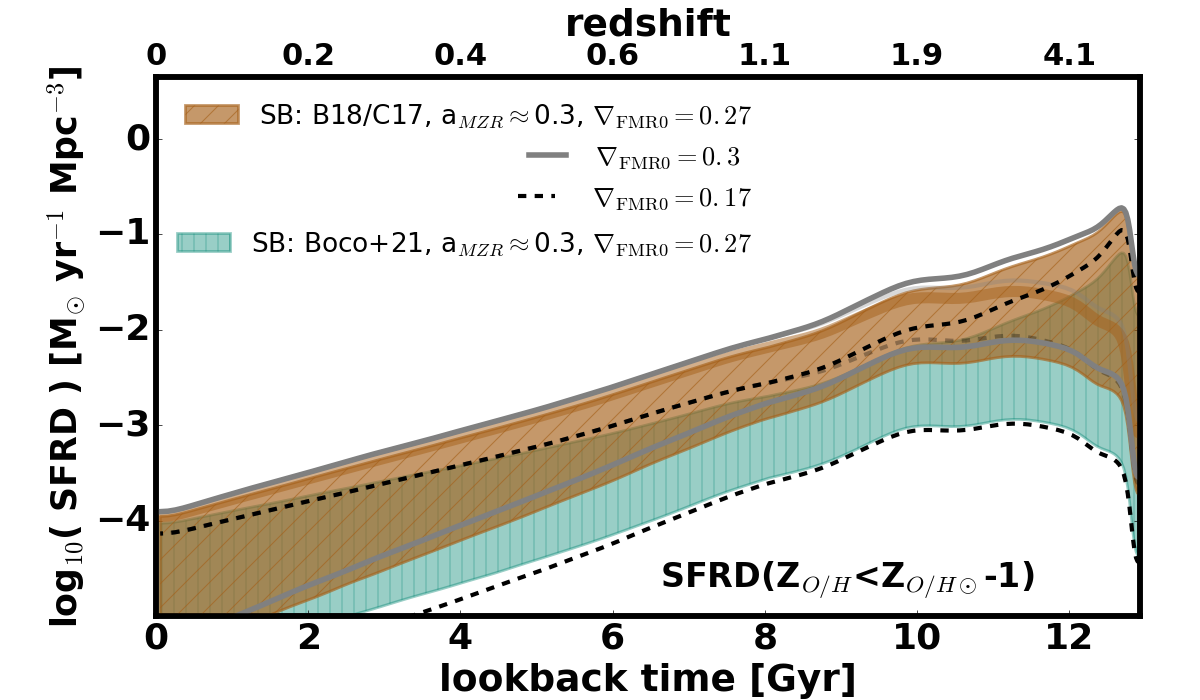
Figure 15: Example illustrating the effect of $\nabla_{\rm FMR0}$ on the low metallicity cut of the cosmic SFH. The brown range shows estimate obtained with B18/C17 starbursts implementation and $a_{\rm MZR}\sim$0.3, assuming $\nabla_{\rm FMR0}$=0.27 (same as in Fig. 12). Gray solid (black dashed) lines mark the location of the upper and lower edges of that range obtained with $\nabla_{\rm FMR0}$=0.3 ( $\nabla_{\rm FMR0}$=0.17). Faint lines in the corresponding colours show the evolution of the upper edge under the assumption of non-evolving low mass end of the GSMF. For comparison, we also show the range obtained with Boco et al. (2021) starbursts implementation, $a_{\rm MZR}\sim$0.3 and $\nabla_{\rm FMR0}$=0.27 (turquoise, same as in Fig. 12). If the SFR-metallicity correlation is much weaker than implied by our fiducial $\nabla_{\rm FMR0}$=0.27, the impact of starbursts on the low metallicity cut of the SFH is substantially reduced.

As discussed in Sec. 3.1.5, the range of extreme reasonable assumptions about $\nabla_{\rm FMR0}$ and the potential dependence of this parameter for instance, on the metallicity derivation technique, cannot be easily identified with the currently available observational results. We therefore discuss the sensitivity of our result to the choice of this factor. The impact of $\nabla_{\rm FMR0}$ on the high and low metallicity cut of the cosmic SFH for the example model variations is shown in Fig. 14 and Fig. 15, respectively. In essence, higher (lower) $\nabla_{\rm FMR0}$ increase (decrease) the amount of SFRD that happens at low metallicity (and vice versa for the SFRD at high metallicity). Lower $\nabla_{\rm FMR0}$ means that the difference between the metallicities of highly star-forming galaxies and their quiescent counterparts of the same mass is reduced. As a consequence, if the anti-correlation between the SFR and metallicity is much weaker than with our fiducial assumptions, the impact of starbursts on the low metallicity cut of the SFH is substancially reduced. This can be seen in Fig. 15, where the lower and upper edges of the range obtained with B18/C17 starburst implementation and $\nabla_{\rm FMR0}$=0.17 (dashed lines) roughly match the range obtained for the corresponding model variations assuming low fraction of starbursts (turquoise range). This also means that the impact of the choice of $\nabla_{\rm FMR0}$ on the variations with lower fraction of starbursts and/or starburst sequence with smaller offset from the SFMR than in B18/C17 implementation, is smaller than in the examples shown in Fig. 15 and 14. As discussed in Sec. 5.1.1, $\nabla_{\rm FMR0}$ also affects the rate of the overall decrease in metallicity - and so the slope of the different metallicity cuts of the cosmic SFH as a function of redshift. However, while many different factors affect the slope of the low metallicity cut of the SFH below the peak of the cosmic SFH (see Sec. 6.2), at high redshifts assumptions about the low mass end of the GSMF clearly dominate the uncertainty in the slope regardless of $\nabla_{\rm FMR0}$.

7 Conclusions

In this study we expand the framework introduced in Chruslinska & Nelemans (2019) to construct the observation-based distribution of the cosmic SFRD at different metallicities and redshifts. We evaluate its uncertainty in light of additional factors that were not discussed in the original study: the redshift-invariant mass-metallicity-SFR relation (FMR), starburst galaxies and the slope of the local mass-metallicity relation. We show that all of those factors have a strong impact on the low metallicity cut of the cosmic SFH - crucial in the discussion of the origin of various energetic transients.
Similarly to Chruslinska & Nelemans (2019), we consider different MZR and SFMR variations to cover the range of possibilities discussed in the literature and explore the realistic extremes of the f_SFR(Z,z). The diversity of observational derivations of the MZR and SFMR stems from differences in the applied metallicity and SFR determination techniques - those differences in the methods also affect the FMR determinations. To ensue the consistency of our method, we develop a phenomenological model to construct the FMR based on the local MZR and SFMR. We introduce a parameter $\nabla_{\rm FMR0}$ to characterise the strength of the SFR-metallicity correlation in the high SFR part of the FMR. That is the only parameter which is not constrained by the choice of $z\sim 0$ MZR and SFMR within our description and we discuss the sensitivity of our results to this factor. Our description captures all characteristic features of the observationally inferred relation. It reproduces the known systematic differences between the FMR derived with various metallicity and SFR determination techniques and predicts dependence of the properties of the FMR on the parameters of the $z\sim 0$ MZR and SFMR that can be verified with future observational studies.
Furthermore, we use the results of Caputi et al. (2017) and Bisigello et al. (2018) to describe the properties of starburst galaxies and include their contribution in our f_SFR(Z,z) models. We contrast the f_SFR(Z,z) derived that way with the f_SFR(Z,z) obtained with the description of starbursts as recently used in Boco et al. (2021) (based on Sargent et al. (2012) and Béthermin et al. (2012), which predict a much smaller contribution of strabursts to the total cosmic SFRD budget). In addition to full f_SFR(Z,z) distributions obtained for different variations of our model, we discuss the resulting cosmic SFH and its low and high metallicity cuts.
Our main conclusions are the following:

• As recently discussed in Boco et al. (2021), a redshift-invariant FMR can lead to drastically different conclusions about the metallicity at which the star formation occurs at $z\gtrsim$3 than the redshift-dependent MZR extrapolated to high redshifts (as used in Chruslinska & Nelemans (2019)). However, while the high metallicity cut of the SFH at $z\gtrsim$3.5 is strongly affected by this assumption (Fig. 13), the low metallicity SFH estimate from Chruslinska & Nelemans (2019) falls within the range covered by the variations explored in this study (Fig. 12). In that case, the much shallower metallicity evolution implied by the non-evolving FMR is counterbalanced by the low metallicity contribution of starbursts (assuming that they follow the same FMR as regular star forming galaxies).

• The low metallicity tail of the f_SFR(Z,z) is the most sensitive to variations in the model assumptions. We find a factor of $\sim$200 ($\sim$40) difference in the amount of SFRD occurring below 10% solar metallicity at $z\sim$0 ($z\sim$2) between the extreme model variations considered in this study.

• At low redshifts, the uncertainty of the low metallicity SFH is dominated by the assumptions about the slope and normalisation of the local MZR, while both MZR and starbursts strongly affect this quantity at $z>1$. However, the importance of starbursts for the low metallicity cut of the SFH is highly sensitive to the assumed strength of the SFR-metallicity correlation ($\nabla_{\rm FMR0}$).

• Beyond the peak of the cosmic SFH, the shape of the low metallicity cut of the SFH (peak location, slope) is set by the assumptions about the low mass end of the GSMF. Those assumptions also dominate the redshift dependence of the total SFRD at $z\gtrsim$3. Given this sensitivity, we propose that a tracer of the SFR happening at low metallicity available at high redshifts (e.g. volumetric rate of long gamma ray bursts, or potentially - stellar black hole mergers) could provide constraints on the contribution of low mass galaxies -difficult to constrain otherwise- to the SFRD at those redshifts.

• The uncertainty in the total SFRD in our models at $z\lesssim 1$ is dominated by the uncertain shape of the high mass end of the SFMR. Assumptions about the contribution of starbursts dominate the uncertainty of the cosmic SFH at $1<z\lesssim 3$. Model variations with SFMR with sharp flattening at high masses, non-evolving low mass slope of the GSMF and no/small fraction of starbursts may underpredict the total SFRD at $z\sim$3. Model variations which account for the contribution of starbursts with B18/C17 based prescription lead to $\sim$2.5 times higher SFRD at $z\gtrsim$4 and shallower redshift evolution of the total SFRD at $z\gtrsim$2, more in line with the recent SFRD determinations at high redshifts.

Data Availability

The results of our calculations (allowing to reproduce all of the results shown in the paper) for all model variations discussed in this study will be made publicly available under this url: https://ftp.science.ru.nl/astro/mchruslinska upon the acceptance of this manuscript.

Appendix A FMR variations - additional figures

In this Section we show additional figures illustrating the sensitivity of Z_O/H(SFR,M_∗) to the parameter $\beta$ (Figure 16) and the Z_O/H(SFR,M_∗) dependence on various choices of the parameters of our observation-based model.
Figure 17 shows the values of $\beta$ as a function of log₁₀(SFR) obtained as described in Sec. 3.1.4 for different choices of the $z\sim 0$ MZR, $\nabla_{\rm FMR0}$ and SFMR used in this study.
Figures 18 and 19 show the comparison between the Z_O/H(SFR,M_∗) obtained for different SFMR and $\nabla_{\rm FMR0}$ choices, respectively.

Figure 16: Dependence on $\beta$ parameter in eq. 1, illustrated using the best fit MZR z$\sim$0 parameters from Curti et al. (2020) and various choices of $\beta$. If $\beta$ can be constrained to values $\beta\gtrsim$1, the $Z_{O/H}$ uncertainty induced by the choice of this parameter is relatively small and affects a relatively small range of galaxy masses. However, if $\beta\lesssim$1, small variation in this parameter can add a appreciable uncertainty to $Z_{O/H}$ .

Figure 17: Parameter $\beta$ as a function of log₁₀(SFR) (see eq. 1), depending on the choice of $z\sim 0$ MZR (different columns), $\nabla_{\rm FMR0}$ (different rows) and the shape of the high mass end of the $z\sim 0$ SFMR (different lines). Single value of $\beta$ provides a good description if the SFMR does not significantly depart from a single power law. See Sec 3.4 for the description of different model variations.

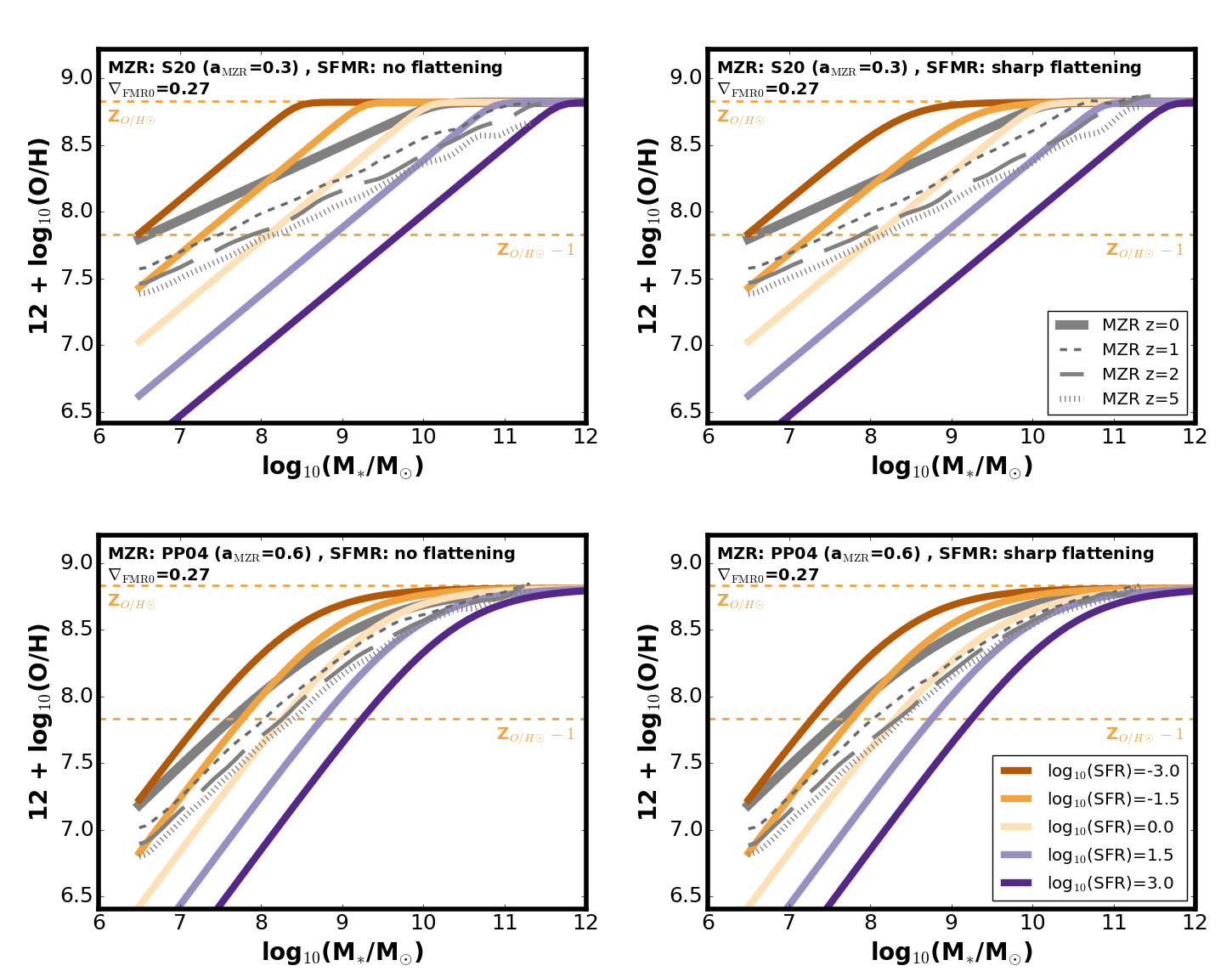
Figure 18: Same as Fig. 4, but for different choices of the $z\sim 0$ SFMR and MZR. Left (right) panels assume SFMR with no (sharp) flattening at the high mass end. Top (bottom) panels assume S20 (PP04) $z\sim 0$ MZR. All panels assume $\nabla_{\rm FMR0}$=0.27.

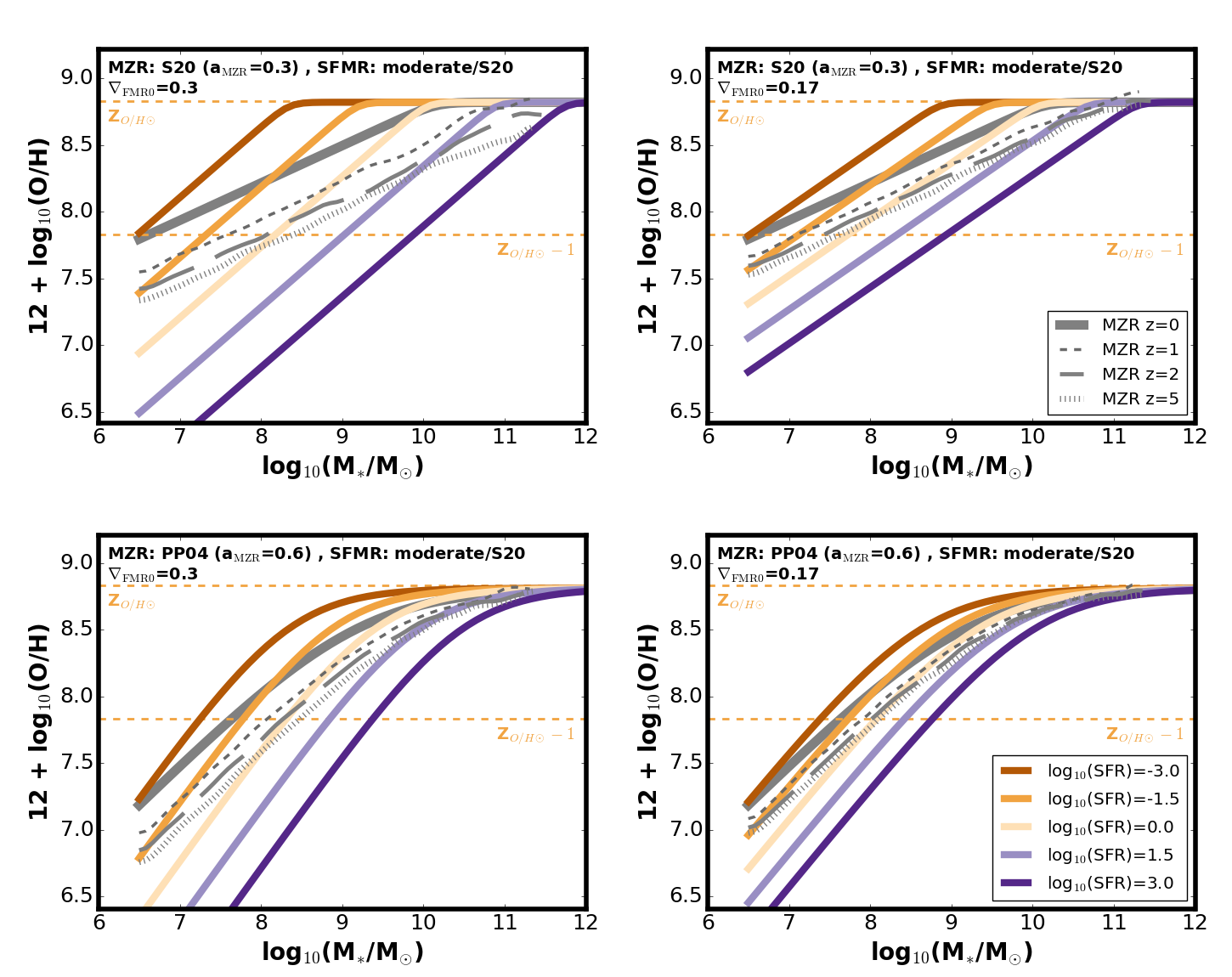
Figure 19: Same as Fig. 4, but for different choices of $\nabla_{\rm FMR0}$. Top (bottom) panels assume S20 (PP04) $z\sim 0$ MZR. All panels assume SFMR with a moderate flattening at high masses (a_SFMR=0.72 at the high mass end).

Appendix B Cosmic SFH - additional materials

Table 4 provides the coefficients of the broken power law fits to the total cosmic SFH for the variations with non-evolving low mass end of the GSMF. Table 5 (6) provides the corresponding coefficients obtained for the low metallicity cut of the cosmic SFH, fitted for the variations with redshift-dependent (non evolving) low mass end of the GSMF.
Figure 20 (21) shows the fraction of the total SFRD that happens below 10% solar metallicity, i.e $Z_{O/H}<Z_{O/H\odot}$-1 (above solar metallicity, i.e. $Z>Z_{O/H}$) as a function of redshift/lookback time, obtained for the different variations of our model discussed in Sec. 6.2 (6.3). Note that those variations in general lead to different total SFRD at different redshift, which also affects the spread between the estimates of the low (high) metallicity part of the cosmic SFH shown in Fig. 12 (13). Fig. 20 allows to directly compare the differences in the low (high) metallicity tail of the f_SFR(Z,z) distribution.

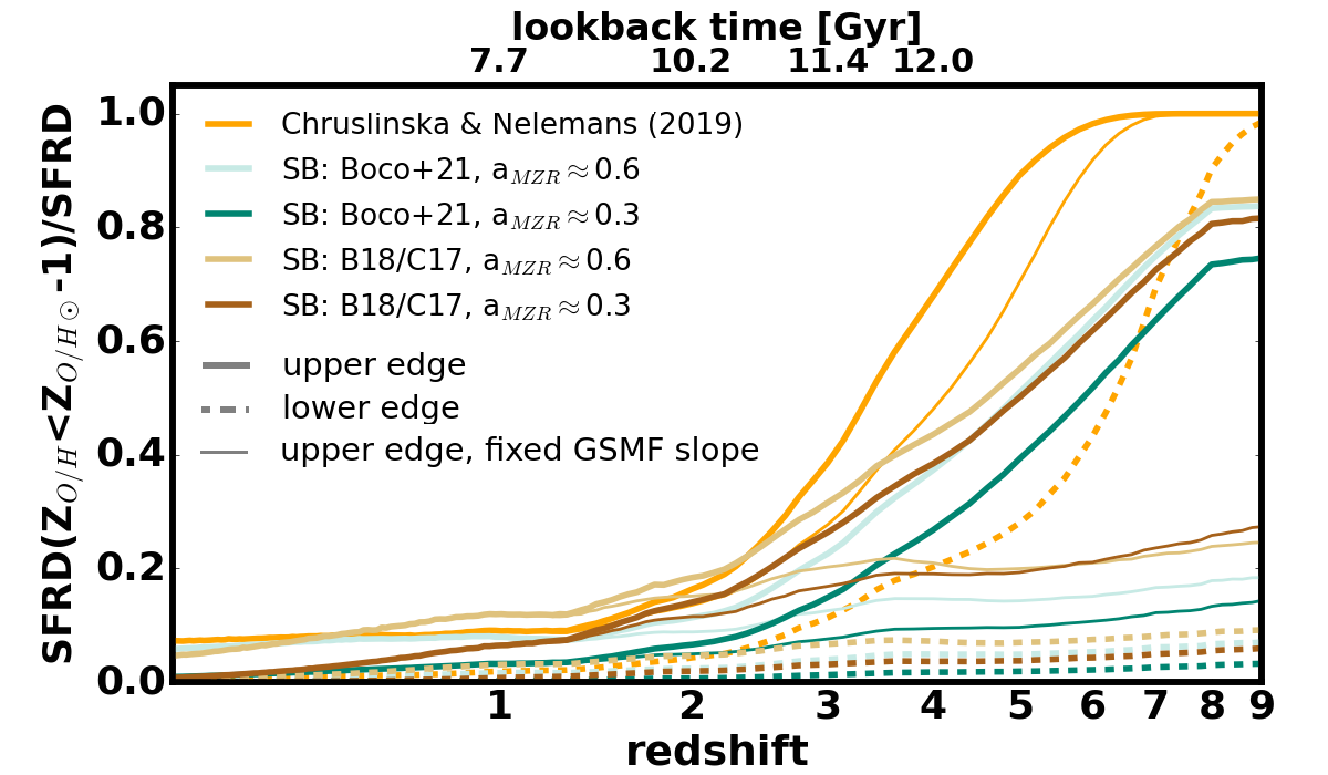
Figure 20: Fraction of the total SFRD that occurs below Z_O/H⊙-1 as a function of redshift/lookback time, plotted for the model variations shown in Fig. 12. Different colours correspond to different assumptions about $a_{MZR}$ and starburst galaxies (see legend). Thick solid (dashed) lines mark the upper (lower) edges of the corresponding ranges for each of the model variations. Thin solid lines show the location of the upper edge obtained under the assumption of a non-evolving low mass end of the GSMF.

Table 4: Same as Table 3, but considering only variations with non-evolving low mass end of the GSMF

cosmic SFH - lower edge ($\alpha_{\rm GSMF}$ fixed)
variation:	no SB		SB: Boco+21		SB: B18/C17
$z$ range	$\kappa$	A	$\kappa$	A	$\kappa$	A
0<$z\leqslant$1.0	2.6307	0.00779	2.5875	0.00924	2.7706	0.0125
1.0<$z\leqslant$1.8	2.3888	0.00922	2.3265	0.0111	2.6969	0.0131
1.8<$z\leqslant$3.0	-1.0535	0.319	-1.1284	0.388	-0.7558	0.458
3.0<$z\leqslant$7.0	-2.2771	1.74	-2.2909	1.95	-1.9628	2.44
7.0<$z\leqslant$8.8	-12.5425	3.24$\cdot 10^{9}$	-12.5526	3.6$\cdot 10^{9}$	-12.4895	7.85$\cdot 10^{9}$
8.8<$z\leqslant$10	0	0.0012	0	0.0013	0	0.00327
cosmic SFH - upper edge ($\alpha_{\rm GSMF}$ fixed)
variation:	no SB		SB: Boco+21		SB: B18/C17
$z$ range	$\kappa$	A	$\kappa$	A	$\kappa$	A
0<$z\leqslant$1.0	2.2211	0.0194	2.2208	0.0209	2.3822	0.0248
1.0<$z\leqslant$1.8	1.8466	0.0251	1.8463	0.027	2.2105	0.028
1.8<$z\leqslant$4.0	-1.7884	1.06	-1.7847	1.14	-1.2278	0.964
4.0<$z\leqslant$7.0	-2.6385	4.16	-2.6376	4.49	-2.4769	7.2
7.0<$z\leqslant$8.8	-12.6417	4.5$\cdot 10^{9}$	-12.6485	4.93$\cdot 10^{9}$	-12.5280	8.6$\cdot 10^{9}$
8.8<$z\leqslant$10	0	0.00133	0	0.00143	0	0.00328

Table 5: Coefficients of the power law fits to the low metallicity cut of the cosmic SFH (lower and upper edges of the ranges shown in Fig. 12) obtained for different variations of our observation-based model. Within each redshift range indicated in the first column total SFRD can be approximated with the dependence: SFRD=A$\cdot(1+z)^{\kappa}[{\rm~{}M}_{\odot}/yr]$.

low metallicity SFH - lower edge
variation:	SB: Boco+21, a${}_{MZR}\sim$0.3		SB: Boco+21, a${}_{MZR}\sim$0.6		SB: B18/C17, a${}_{MZR}\sim$0.3		SB: B18/C17, a${}_{MZR}\sim$0.6
$z$ range	$\kappa$	A	$\kappa$	A	$\kappa$	A	$\kappa$	A
0$<z\leqslant$0.5	6.4712	2.912$\cdot 10^{-6}$	3.8153	1$\cdot 10^{-4}$	8.3323	4.519$\cdot 10^{-6}$	4.8660	1$\cdot 10^{-4}$
0.5$<z\leqslant$1	6.1722	3.287$\cdot 10^{-6}$	3.9229	1.036$\cdot 10^{-4}$	6.8234	8.331$\cdot 10^{-6}$	4.7246	1.5941$\cdot 10^{-4}$
1$<z\leqslant$1.8	4.7030	9.101$\cdot 10^{-6}$	2.9237	2.071$\cdot 10^{-4}$	4.8817	3.2$\cdot 10^{-5}$	3.4034	3.9821$\cdot 10^{-4}$
1.8$<z\leqslant$7	-0.6499	2.253$\cdot 10^{-3}$	-1.0032	0.01181	-0.6698	9.719$\cdot 10^{-3}$	-0.9736	0.3608
7$<z\leqslant$8.8	-11.888	3.172$\cdot 10^{7}$	-12.176	1.455$\cdot 10^{8}$	-11.931	1.437$\cdot 10^{8}$	-12.1147	4.1571$\cdot 10^{8}$
8.8$<z\leqslant$10	0	5.225$\cdot 10^{-5}$	0	1.239$\cdot 10^{-4}$	0	2.144$\cdot 10^{-4}$	0	4.0771$\cdot 10^{-4}$
low metallicity SFH - upper edge
variation:	SB: Boco+21, a${}_{MZR}\sim$0.3		SB: Boco+21, a${}_{MZR}\sim$0.6		SB: B18/C17, a${}_{MZR}\sim$0.3		SB: B18/C17, a${}_{MZR}\sim$0.6
$z$ range	$\kappa$	A	$\kappa$	A	$\kappa$	A	$\kappa$	A
0$<z\leqslant$0.5	4.4163	9.410$\cdot 10^{-5}$	2.9836	6$\cdot 10^{-4}$	5.9088	1.149$\cdot 10^{-4}$	4.0787	6$\cdot 10^{-4}$
0.5$<z\leqslant$1	4.2247	1.017$\cdot 10^{-4}$	3.0826	5.389$\cdot 10^{-4}$	5.3151	1.462$\cdot 10^{-4}$	4.1063	6.262$\cdot 10^{-4}$
1$<z\leqslant$1.5	3.9141	1.261$\cdot 10^{-4}$	2.7905	6.599$\cdot 10^{-4}$	4.8008	2.088$\cdot 10^{-4}$	3.7273	8.143$\cdot 10^{-4}$
1.5$<z\leqslant$7	2.4934	4.636$\cdot 10^{-4}$	2.0535	1.296$\cdot 10^{-3}$	2.0328	2.638$\cdot 10^{-3}$	1.8127	4.707$\cdot 10^{-3}$
7$<z\leqslant$8.8	-8.5779	4.619$\cdot 10^{6}$	-8.7763	7.816$\cdot 10^{6}$	-8.896	1.954$\cdot 10^{7}$	-8.9519	2.478$\cdot 10^{7}$
8.8$<z\leqslant$10	0	0.01452	0	0.01562	0	0.02972	0	0.03317

Table 6: Coefficients of the power law fits to the low metallicity cut of the cosmic SFH (lower and upper edges of the ranges as in Fig. 12) obtained for different variations of our observation-based model under the assumption of a non-evolving low mass end of the GSMF. Within each redshift range indicated in the first column total SFRD can be approximated with the dependence: SFRD=A$\cdot(1+z)^{\kappa}[{\rm~{}M}_{\odot}/yr]$.

low metallicity SFH - lower edge
variation:	SB: Boco+21, a${}_{MZR}\sim$0.3		SB: Boco+21, a${}_{MZR}\sim$0.6		SB: B18/C17, a${}_{MZR}\sim$0.3		SB: B18/C17, a${}_{MZR}\sim$0.6
$z$ range	$\kappa$	A	$\kappa$	A	$\kappa$	A	$\kappa$	A
0$<z\leqslant$0.5	6.0172	4.393$\cdot 10^{-6}$	3.3024	1.667$\cdot 10^{-4}$	7.9464	6.561$\cdot 10^{-6}$	4.3940	2.085$\cdot 10^{-4}$
0.5$<z\leqslant$1	5.5287	5.355$\cdot 10^{-6}$	3.3306	1.635$\cdot 10^{-4}$	6.1805	1.343$\cdot 10^{-5}$	4.2022	2.381$\cdot 10^{-4}$
1$<z\leqslant$1.7	4.7328	9.297$\cdot 10^{-6}$	2.8406	2.297$\cdot 10^{-4}$	5.0089	3.024$\cdot 10^{-5}$	3.4101	4.123$\cdot 10^{-4}$
1.7$<z\leqslant$3.5	0.4510	6.537$\cdot 10^{-4}$	-0.0495	0.004053	0.4466	0.002809	0.0103	0.01207
3.5$<z\leqslant$7	-1.8116	0.01965	-2.2411	0.1095	-1.8350	0.08689	-2.2043	0.3376
7$<z\leqslant$8.8	-11.8876	2.471$\cdot 10^{7}$	-12.177	1.028$\cdot 10^{8}$	-11.9308	1.139$\cdot 10^{8}$	-12.115	3.009$\cdot 10^{8}$
8.8$<z\leqslant$10	0	4.069$\cdot 10^{-5}$	0	8.754$\cdot 10^{-5}$	0	1.699$\cdot 10^{-4}$	0	2.951$\cdot 10^{-4}$
low metallicity SFH - upper edge
variation:	SB: Boco+21, a${}_{MZR}\sim$0.3		SB: Boco+21, a${}_{MZR}\sim$0.6		SB: B18/C17, a${}_{MZR}\sim$0.3		SB: B18/C17, a${}_{MZR}\sim$0.6
$z$ range	$\kappa$	A	$\kappa$	A	$\kappa$	A	$\kappa$	A
0$<z\leqslant$0.5	4.4163	9.410$\cdot 10^{-5}$	2.9836	5.772$\cdot 10^{-4}$	5.9088	1.149$\cdot 10^{-4}$	4.0787	6.383$\cdot 10^{-4}$
0.5$<z\leqslant$1	4.2247	1.017$\cdot 10^{-4}$	3.0826	5.389$\cdot 10^{-4}$	5.3151	1.462$\cdot 10^{-4}$	4.1063	6.262$\cdot 10^{-4}$
1$<z\leqslant$1.7	3.6167	1.55$\cdot 10^{-4}$	2.6761	7.143$\cdot 10^{-4}$	4.4986	2.575$\cdot 10^{-4}$	3.5242	9.374$\cdot 10^{-4}$
1.7$<z\leqslant$3.5	0.1790	0.004712	-0.1177	0.01146	0.4267	0.0147	0.0785	0.02873
3.5$<z\leqslant$7	-2.0303	0.1307	-2.3001	0.3052	-1.9322	0.5106	-2.2568	0.9633
7$<z\leqslant$8.8	-12.0388	1.429$\cdot 10^{8}$	-12.1984	2.653$\cdot 10^{8}$	-12.0147	6.509$\cdot 10^{8}$	-12.1707	8.648$\cdot 10^{8}$
8.8$<z\leqslant$10	0	1.666$\cdot 10^{-4}$	0	2.149$\cdot 10^{-4}$	0	8.02$\cdot 10^{-4}$	0	7.464$\cdot 10^{-4}$

Appendix C Z_O/H(SFR, M_∗) implementation with SFR-dependent $\nabla_{\rm FMR}$ (and $\gamma$)

As discussed in Sec. 3.1, Z_O/H(SFR, M_∗) at fixed SFR and M${}_{*}<M_{\rm 0;SFR}$ appear as lines roughly parallel to each other (see examples in, e.g. Mannucci et al. 2010, Telford et al. 2016, Cresci et al. 2019) and we assume that the Z_O/H(SFR, M_∗) slope $\gamma$ is independent of SFR/M_∗. However, in their recent study Curti et al. (2020) fit the slopes of Z_O/H(SFR, M_∗) in individual log₁₀(SFR) bins and indicate a possible dependence of $\gamma$ on SFR. They find that $\gamma$ decreases with decreasing SFR, reaching the value close to that of $\sim$0 MZR slope at low SFR (see figure 9 therein). When Z_O/H(SFR, M_∗) is extrapolated down to low (specific) SFR values, such dependence leads to considerably higher metallicity of galaxies with the lowest masses (M${}_{*}\lesssim 10^{8}{\rm~{}M}_{\odot}$), and therefore can affect the low metallicity tail of the f_SFR(Z,z) distribution obtained with our model.
We explore additional variation of our model to illustrate the effect of such a dependence on our results. Within our description we can model a similar dependence of $\gamma$ on SFR to that found by Curti et al. (2020) by implementing a SFR-dependent $\nabla_{\rm FMR}$ (and therefore of $\gamma$, see e.q. 5) and requiring that the strength of the correlation weakens towards low SFRs, eventually disappearing at a certain low SFR (where $\gamma$ approaches the slope of the z$\sim$0 MZR). As discussed in Sec. 3.1.5, there is some observational evidence for the weakening of the SFR-metallicity correlation below a certain specific SFR threshold ($\rm\lesssim 10^{-10}/yr$, but it should be noted that this behaviour is difficult to constrain at low M${}_{*}\lesssim 10^{8.5}{\rm~{}M}_{\odot}$). For simplicity, we assume that there is a linear dependence of $\nabla_{\rm FMR}$ on log₁₀(SFR), such that at log₁₀(SFR)$\geqslant$log₁₀ (SFR_∇0) $\nabla_{\rm FMR}$ = $\nabla_{\rm FMR0}$ and at log₁₀(SFR)$\leqslant$ log₁₀(SFR${}_{\rm no\ corr.}$) $\nabla_{\rm FMR}$=0. We set log₁₀(SFR${}_{\rm no\ corr.}$)=-2, which roughly corresponds to the SFR of M${}_{*}\sim 10^{8}{\rm~{}M}_{\odot}$ galaxies according to our z$\sim$0 SFMR. We note that below that mass and SFR the observational FMR is not constrained , and by assuming that for those galaxies the correlation disappears we obtain a conservative estimate of the low metallicity contribution of low mass galaxies. Results of our calculations are also sensitive to the value of the SFR threshold above which $\gamma$ is fixed: the higher the value of log₁₀ (SFR_∇0), the lower the amount of the SFRD happening at low metallicity. The choice of this value is unclear and for the illustrative purposes we show our results using two example thresholds: log₁₀ (SFR_∇0)=0 and log₁₀ (SFR_∇0)=1. The resulting Z_O/H(SFR, M_∗) is illustrated in Fig. 22 using the latter threshold and for the different z$\sim$0 MZR choices considered in our study.
The overall f_SFR(Z,z) distribution is only mildly affected by the explored variations with SFR-dependent $\nabla_{\rm FMR}$ (see Fig. 23, the effect is analogous for the variations with the starburst implementation following Boco et al.). The redshift evolution of the peak metallicity is indistinguishable from that estimated with a fixed $\nabla_{\rm FMR}=\nabla_{\rm FMR0}$ case and the only visible difference is in the extent of the low metallicity tail of the distribution (the fixed $\nabla_{\rm FMR}$ case leads to more extended low metallicity tail).
With the low metallicity threshold of 10% solar metallicity (oxygen abundance) used in our study, the difference in the amount of the total SFRD happening at low metallicity estimated in the model variations with fixed and SFR-dependent $\nabla_{\rm FMR}$ is amplified in the cases with flat z$\sim$0 MZR (a${}_{\rm MZR}\sim$0.3) and high MZR normalisation (compare lower edge of the dark brown range and the lower thick dark brown lines in Fig. 25 - note that the strength of this effect is very sensitive to the exact choice of the low metallicity threshold). In those cases the result is particularly sensitive to the assumed low mass/SFR FMR extrapolation, as at low redshifts only galaxies that are MZR outliers have metallicities falling below $Z_{O/H}<Z_{O/H\odot}$-1 (see top left panel in Fig. 22). If there is no correlation between the SFR and metallicity at low SFRs, this leads to a negligible amount of SFRD happening below 10% solar metallicity at low to intermediate redshifts.

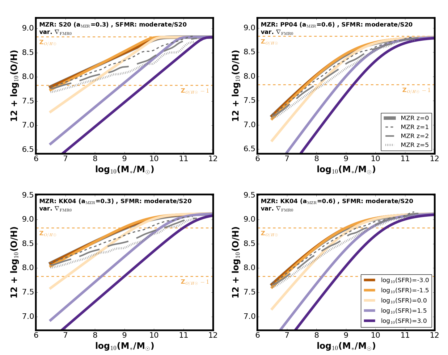
Figure 22: Same as Fig. 4, but assuming a SFR-dependent $\nabla_{\rm FMR}$ (leading to SFR-dependent $\gamma$). Top (bottom) panels assume S20 (PP04) $z\sim 0$ MZR. All panels assume SFMR with a moderate flattening at high masses (a_SFMR=0.72 at the high mass end), log₁₀ (SFR_∇0)=1 and $\nabla_{\rm FMR0}$=0.27.

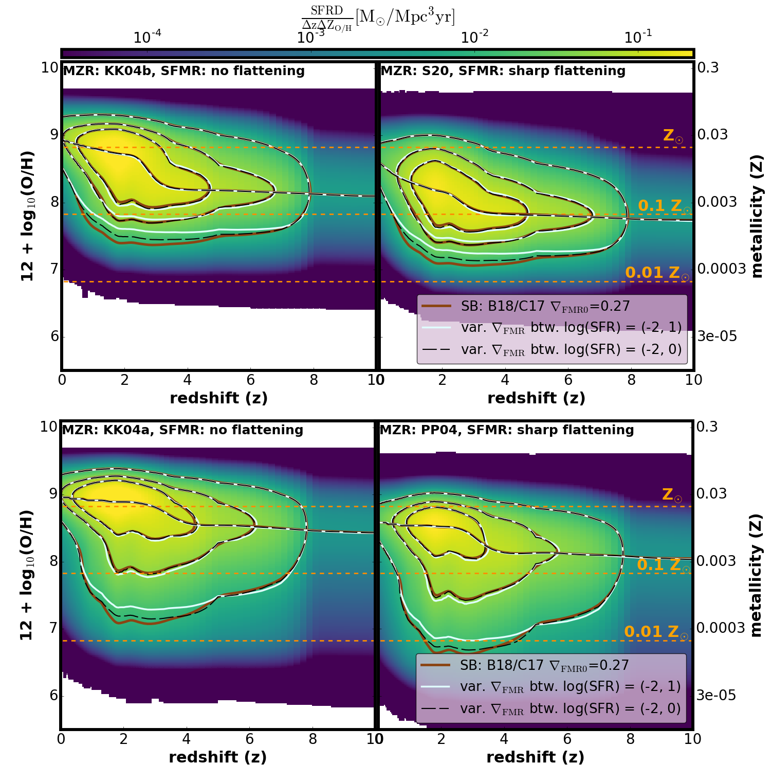
Figure 23: Distribution of the cosmic SFRD at different metallicities and redshift for different Z_O/H(SFR, M_∗) implementations, shown for B18/C17 starbursts implementation (effect is analogous for the starburst implementation following Boco et al. (2021)). Brown contours and background colours correspond to Z_O/H(SFR, M_∗) with a fixed $\nabla_{\rm FMR0}=0.27$. Solid white (dashed black) contours correspond to Z_O/H(SFR, M_∗) modelled with $\nabla_{\rm FMR}$ varying between log₁₀ (SFR)=-2 and log₁₀ (SFR)=1 (log₁₀ (SFR)=0) as described in Sec. C.
Different panels correspond to different z$\sim$0 MZR and SFMR variations (same as in Fig. 9). Contours indicate constant SFRD and are plotted for 0.01,0.05 and 0.1 [ ${\rm~{}M}_{\odot}$/Mpc³ yr] (with the highest value corresponding to the innermost contour). The alternative Z_O/H(SFR, M_∗) implementation has a relatively small effect on the overall distribution, but leads to a less extended low metallicity tail.

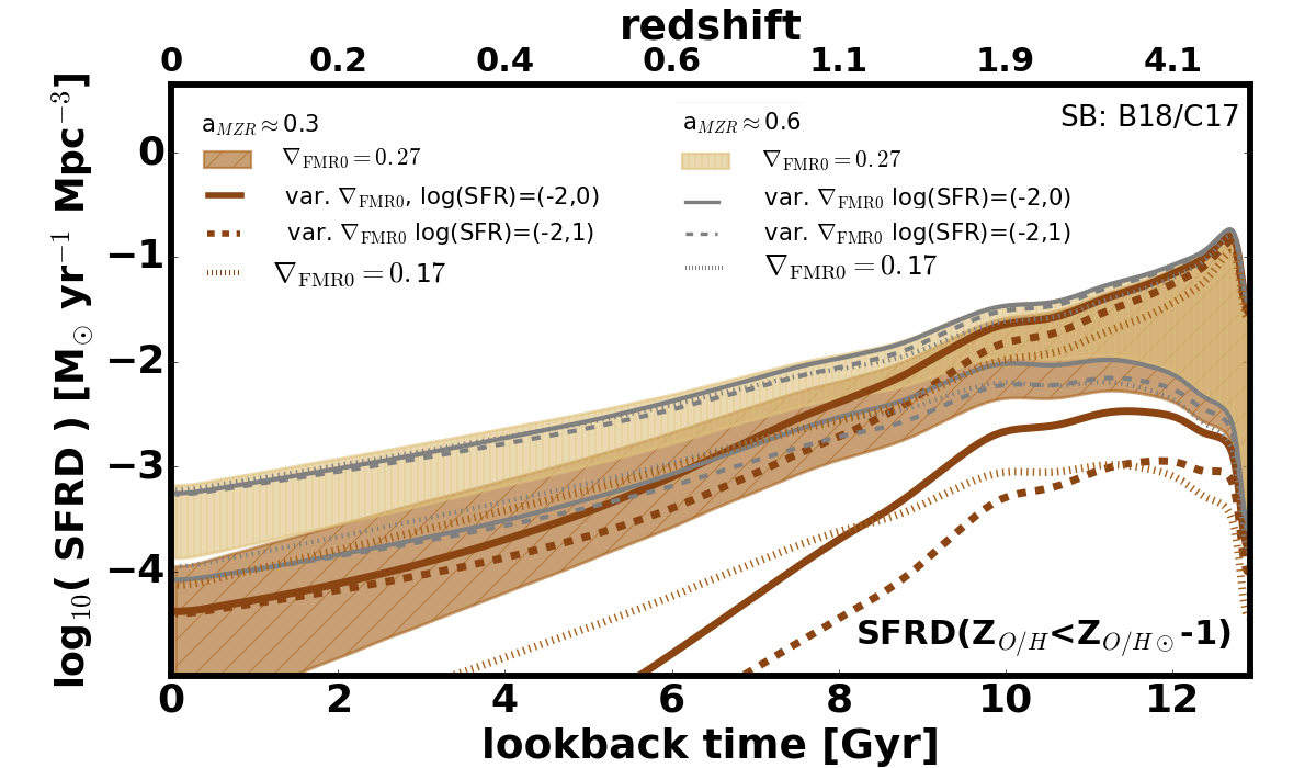
Figure 24: SFRD happening below 10% solar metallicity ($Z_{O/H}<Z_{O/H\odot}$-1) as a function of lookback time/redshift estimated with different Z_O/H(SFR, M_∗) implementations, shown for B18/C17 starbursts implementation (effect is analogous for the starburst implementation following Boco et al. (2021)). The light and dark brown coloured ranges are the same as in Fig. 12 and correspond to a fixed $\nabla_{\rm FMR0}=0.27$ and a${}_{\rm MZR}\approx$0.3 and a${}_{\rm MZR}\approx$0.6 respectively. Dotted gray/brown lines indicate upper and lower edges of the corresponding ranges obtained with $\nabla_{\rm FMR0}=0.17$. Solid (log₁₀ (SFR_∇0)=0) and dashed (log₁₀ (SFR_∇0)=1) lines indicate the upper and lower edges of those ranges obtained with a SFR-dependent $\nabla_{\rm FMR}$ (leading to SFR-dependent $\gamma$, see Sec. C).

Figure 25: Fraction of the total SFRD happening below 10% solar metallicity ($Z_{O/H}<Z_{O/H\odot}$-1) as a function of lookback time/redshift estimated with different Z_O/H(SFR, M_∗) implementations, shown for B18/C17 starbursts implementation (effect is analogous for the starburst implementation following Boco et al. (2021)). Top panel shows the estimates obtained for the low metallicity variations (i.e. corresponding to upper edges in Fig. 25), bottom panel shows the estimates obtained for the high metallicity variations. The green (purple) ranges span between the estimates obtained with Z_O/H(SFR, M_∗) with a fixed $\nabla_{\rm FMR0}=0.3$ and 0.17 and a${}_{\rm MZR}\approx$0.3 (a${}_{\rm MZR}\approx$0.6). Different lines indicate the corresponding estimate obtained with Z_O/H(SFR, M_∗) with a SFR-dependent $\nabla_{\rm FMR}$, varying between log₁₀ (SFR)=-2 and log₁₀(SFR)=0 or 1 (see legend and Sec. C).

References

- Andrews & Martini (2013) Andrews B. H., Martini P., 2013, ApJ, 765, 140
- Belczynski et al. (2016) Belczynski K., Holz D. E., Bulik T., O’Shaughnessy R., 2016, Nature, 534, 512
- Bensby et al. (2004) Bensby T., Feltzing S., Lundström I., 2004, A&A, 415, 155
- Béthermin et al. (2012) Béthermin M., et al., 2012, ApJ, 757, L23
- Bisigello et al. (2018) Bisigello L., Caputi K. I., Grogin N., Koekemoer A., 2018, A&A, 609, A82
- Boco et al. (2019) Boco L., Lapi A., Goswami S., Perrotta F., Baccigalupi C., Danese L., 2019, ApJ, 881, 157
- Boco et al. (2021) Boco L., Lapi A., Chruslinska M., Donevski D., Sicilia A., Danese L., 2021, ApJ, 907, 110
- Boogaard et al. (2018) Boogaard L. A., et al., 2018, A&A, 619, A27
- Bothwell et al. (2013) Bothwell M. S., Maiolino R., Kennicutt R., Cresci G., Mannucci F., Marconi A., Cicone C., 2013, MNRAS, 433, 1425
- Broekgaarden et al. (2021) Broekgaarden F. S., et al., 2021, arXiv e-prints, p. arXiv:2103.02608
- Caputi et al. (2017) Caputi K. I., et al., 2017, ApJ, 849, 45
- Casey et al. (2018) Casey C. M., et al., 2018, ApJ, 862, 77
- Chruslinska & Nelemans (2019) Chruslinska M., Nelemans G., 2019, MNRAS, 488, 5300
- Chruslinska et al. (2019) Chruslinska M., Nelemans G., Belczynski K., 2019, MNRAS, 482, 5012
- Chruślińska et al. (2020) Chruślińska M., Jeřábková T., Nelemans G., Yan Z., 2020, A&A, 636, A10
- Cresci et al. (2019) Cresci G., Mannucci F., Curti M., 2019, A&A, 627, A42
- Cullen et al. (2021) Cullen F., et al., 2021, MNRAS, 505, 903
- Curti et al. (2020) Curti M., Mannucci F., Cresci G., Maiolino R., 2020, MNRAS, 491, 944
- Davé et al. (2011) Davé R., Finlator K., Oppenheimer B. D., 2011, MNRAS, 416, 1354
- De Lucia et al. (2020) De Lucia G., Xie L., Fontanot F., Hirschmann M., 2020, MNRAS, 498, 3215
- De Rossi et al. (2017) De Rossi M. E., Bower R. G., Font A. S., Schaye J., Theuns T., 2017, MNRAS, 472, 3354
- Ellison et al. (2008) Ellison S. L., Patton D. R., Simard L., McConnachie A. W., 2008, ApJ, 672, L107
- Giacobbo et al. (2018) Giacobbo N., Mapelli M., Spera M., 2018, MNRAS, 474, 2959
- Gräfener & Hamann (2008) Gräfener G., Hamann W. R., 2008, A&A, 482, 945
- Grevesse & Sauval (1998) Grevesse N., Sauval A. J., 1998, Space Sci. Rev., 85, 161
- Gruppioni et al. (2020) Gruppioni C., et al., 2020, A&A, 643, A8
- Hunt et al. (2012) Hunt L., et al., 2012, MNRAS, 427, 906
- Hunt et al. (2016) Hunt L., Dayal P., Magrini L., Ferrara A., 2016, MNRAS, 463, 2002
- Ilbert et al. (2015) Ilbert O., et al., 2015, A&A, 579, A2
- Kashino et al. (2016) Kashino D., Renzini A., Silverman J. D., Daddi E., 2016, ApJ, 823, L24
- Kewley & Ellison (2008) Kewley L. J., Ellison S. L., 2008, ApJ, 681, 1183
- Khusanova et al. (2021) Khusanova Y., et al., 2021, A&A, 649, A152
- Klencki et al. (2018) Klencki J., Moe M., Gladysz W., Chruslinska M., Holz D. E., Belczynski K., 2018, A&A, 619, A77
- Kobulnicky & Kewley (2004) Kobulnicky H. A., Kewley L. J., 2004, ApJ, 617, 240
- Kroupa (2001) Kroupa P., 2001, MNRAS, 322, 231
- Lagos et al. (2016) Lagos C. d. P., et al., 2016, MNRAS, 459, 2632
- Lara-López et al. (2010) Lara-López M. A., et al., 2010, A&A, 521, L53
- Loiacono et al. (2021) Loiacono F., et al., 2021, A&A, 646, A76
- Madau & Dickinson (2014) Madau P., Dickinson M., 2014, ARA&A, 52, 415
- Maiolino & Mannucci (2019) Maiolino R., Mannucci F., 2019, A&ARv, 27, 3
- Maiolino et al. (2008) Maiolino R., et al., 2008, A&A, 488, 463
- Mannucci et al. (2009) Mannucci F., et al., 2009, MNRAS, 398, 1915
- Mannucci et al. (2010) Mannucci F., Cresci G., Maiolino R., Marconi A., Gnerucci A., 2010, MNRAS, 408, 2115
- Mannucci et al. (2011) Mannucci F., Salvaterra R., Campisi M. A., 2011, MNRAS, 414, 1263
- Neijssel et al. (2019) Neijssel C. J., et al., 2019, MNRAS, 490, 3740
- Orlitova (2020) Orlitova I., 2020, arXiv e-prints, p. arXiv:2012.12378
- Pearson et al. (2018) Pearson W. J., et al., 2018, A&A, 615, A146
- Pettini & Pagel (2004) Pettini M., Pagel B. E. J., 2004, MNRAS, 348, L59
- Renzini & Peng (2015) Renzini A., Peng Y.-j., 2015, ApJ, 801, L29
- Rodighiero et al. (2011) Rodighiero G., et al., 2011, ApJ, 739, L40
- Salim et al. (2014) Salim S., Lee J. C., Ly C., Brinchmann J., Davé R., Dickinson M., Salzer J. J., Charlot S., 2014, ApJ, 797, 126
- Sanders et al. (2018) Sanders R. L., et al., 2018, ApJ, 858, 99
- Sanders et al. (2020) Sanders R. L., et al., 2020, arXiv e-prints, p. arXiv:2009.07292
- Sargent et al. (2012) Sargent M. T., Béthermin M., Daddi E., Elbaz D., 2012, ApJ, 747, L31
- Schreiber et al. (2015) Schreiber C., et al., 2015, A&A, 575, A74
- Speagle et al. (2014) Speagle J. S., Steinhardt C. L., Capak P. L., Silverman J. D., 2014, ApJS, 214, 15
- Steidel et al. (2016) Steidel C. C., Strom A. L., Pettini M., Rudie G. C., Reddy N. A., Trainor R. F., 2016, ApJ, 826, 159
- Telford et al. (2016) Telford O. G., Dalcanton J. J., Skillman E. D., Conroy C., 2016, ApJ, 827, 35
- Tolstoy et al. (2009) Tolstoy E., Hill V., Tosi M., 2009, ARA&A, 47, 371
- Tomczak et al. (2016) Tomczak A. R., et al., 2016, ApJ, 817, 118
- Topping et al. (2020) Topping M. W., Shapley A. E., Reddy N. A., Sanders R. L., Coil A. L., Kriek M., Mobasher B., Siana B., 2020, MNRAS, 499, 1652
- Torrey et al. (2018) Torrey P., et al., 2018, MNRAS, 477, L16
- Torrey et al. (2019) Torrey P., et al., 2019, MNRAS, 484, 5587
- Vink & de Koter (2005) Vink J. S., de Koter A., 2005, A&A, 442, 587
- Vink et al. (2001) Vink J. S., de Koter A., Lamers H. J. G. L. M., 2001, A&A, 369, 574
- Wheeler et al. (1989) Wheeler J. C., Sneden C., Truran Jr. J. W., 1989, ARA&A, 27, 279
- Yabe et al. (2015) Yabe K., et al., 2015, PASJ, 67, 102
- Yates et al. (2012) Yates R. M., Kauffmann G., Guo Q., 2012, MNRAS, 422, 215
- Zahid et al. (2014a) Zahid H. J., Dima G. I., Kudritzki R.-P., Kewley L. J., Geller M. J., Hwang H. S., Silverman J. D., Kashino D., 2014a, ApJ, 791, 130
- Zahid et al. (2014b) Zahid H. J., et al., 2014b, ApJ, 792, 75