Single-stream CNN with Learnable
Architecture for Multi-source
Remote Sensing Data

Abstract

In this paper, we propose an efficient and generalizable framework based on deep convolutional neural network (CNN) for multi-source remote sensing data joint classification. While recent methods are mostly based on multi-stream architectures, we use group convolution to construct equivalent network architectures efficiently within a single-stream network. Based on a recent technique called dynamic grouping convolution, We further propose a network module named SepDGConv, to make group convolution hyperparameters, and thus the overall network architecture, learnable during network training. In the experiments, the proposed method is applied to ResNet and UNet, and the adjusted networks are verified on three very diverse benchmark data sets (i.e., Houston2018 data, Berlin data, and MUUFL data). Experimental results demonstrate the effectiveness of the proposed single-stream CNNs, and in particular SepG-ResNet18 improves the state-of-the-art classification overall accuracy (OA) on HS-SAR Berlin data set from $62.23\%$ to $68.21\%$. In the experiments we have two interesting findings. First, using DGConv generally reduces test OA variance. Second, multi-stream is harmful to model performance if imposed to the first few layers, but becomes beneficial if applied to deeper layers. Altogether, the findings imply that multi-stream architecture, instead of being a strictly necessary component in deep learning models for multi-source remote sensing data, essentially plays the role of model regularizer. Our code is publicly available at https://github.com/yyyyangyi/Multi-source-RS-DGConv. We hope our work can inspire novel research in the future.

I Introduction

Remote sensing (RS) plays an important role in earth observation, and supports applications such as environmental monitoring [1], precision agriculture [2], etc. One fundamental yet challenging task in RS is land-use/land-cover (LULC) classification, which aims to assign one semantic category to each pixel in an RS image acuqired over some region of interest.

Nowadays, diverse sensor technologies allow to measure different aspects of scenes and objects from the air, including sensors for multispectral (MS) optical imaging, hyperspectral (HS) imaging, synthetic aperture radar (SAR), and light detection and ranging (LiDAR). Different sensors bring diverse and complementary information [3]. For example, MS optical imagery contains spatial information such as object shape and spatial relationship. HS data provides detailed spectral information of LULC and ground objects. While HS imagery cannot be used to differentiate objects composed of the same material, such as roofs and roads both made of concrete, LiDAR data can capture elevation distribution and thus can be used to distinguish roofs from roads. And SAR data can provide additional structure information about Earth’s surface. Availability of multi-source, multi-modal RS data makes it possible to integrate rich information to improve LULC classification performance. And considerable efforts have been invested into the research of multi-source RS data joint analysis for LULC since recent years.

I-A Related work

Conventionally, multi-source RS data analysis workflow contains two phases: one feature extraction phase, and one feautre fusion phase. In feature extraction phase, different feature extractors are applied to different data modalities, while in feature fusion phase, high level features obtained from the previous phase are fused by certain algorithms and fed to LULC classifiers. For example, both [4] [5] extract morphological attribute profiles from HS and LiDAR data, and use feature stacking as a fusion technique. In [6], morphological extinction profiles are extracted seperately from HS and LiDAR data, and the features are further fused using orthogonal TV component analysis (OTVCA). In [7], the authors extract manually engineered features from MS and LiDAR data, and use multiple kernel learning as a fusion strategy to train a support vector machine classifier. In [8], MAPPER [9] is used as a feature extractor for MS optical and SAR data, and the features are further fused with manifold alignment. Note that, in the literature, data fusion also refers to a data processing technique that integrates multi-source data into one data modality, while in our paper we use this term to express the same meaning as ”joint classification / analysis” of multi-source RS data.

Meanwhile, deep learning (DL) [10], as one of the most notable advances in computer vision (CV) recently, has attracted attention from both CV and RS communities. In particular, convolutional neural network (CNN) [11] is a DL based model that significantly outperforms traditional methods in image classification and segmentation. Most of the data in RS is also presented in the form of images, and CNN has shown remarkable success in analyzing MS [12] [13] [14], HS [15] [16] [17], LiDAR [18] [19], and SAR data [20] [21].

Besides being applied to individual data sources, CNNs are adopted as backbone models for multi-source RS data classification in many recent works. As an early attempt, [22] designs a two-branch CNN for joint analysis of HS-LiDAR data, one branch for each sensor, achieving promising classification accuracy. [23] proposes another two-branch CNN for HS-LiDAR data, with a different design of HS feature extraction branch. In [24], a three-branch CNN is proposed to fuse MS, HS and LiDAR data. [25] further extend the scope of deep multi-branch networks by allowing either CNN or fully connected neural networks be one feature extraction branch. See Sec. II(A) for a formal definition of network branch.

Based on the multi-branch architecture, some latest papers devote to further improve model performance by introducing various novel modules to the network. In [26], the authors use self-adversarial modules, interactive learning modules and label propagation modules to build a deep CNN for semi-supervised multi-modal learning. In [27], Gram matrices are utilized to improve multisource complementary information preservation in a two-branch CNN for HS and LiDAR data fusion. In [28], a two-branch CNN for joint classification of HS and LiDAR is proposed, where in the feature extraction branches Octave convolutional layers are used to reduce feature redundancy from low-frequency data components, and in the fusion sub-network fractional Gabor convolution is utilized to obtain multiscale and multidirectional spatial features.

Using multi-stream architectures as above, this data fusion strategy is also known as the ”late-fusion” scheme, since the features are kept sensor-specific until the last few layers, i.e., the fusion sub-network. Another strategy in contrast to late-fusion is ”early-fusion”. As the name suggests, early-fusion means either the feature extraction branches are very shallow, or there are certain information exchange between different branches, making the features no longer absolutely sensor-specific. In [29], a coupled CNN is proposed to fuse HS and LiDAR data, where weight sharing technique is utilized in intermediate layers of the proposed two-branch CNN, making each feature extraction branch only contain very few separate layers. [30] proposes a fully convolutional neural network named FuseNet with two branches for semantic labeling of indoor scenes on RGB-D data. To fuse features from RGB branch and depth branch, the authors propose a fusion block, which adds the output of each block from depth branch to RGB branch. In [31] a more detained comparison between FuseNet based early fusion and multi-branch late fusion is made, and the authors find out that one strategy does not consistently outperform the other on different data sets. In [32], MS optical data and a digital surface model (DSM) band is jointly classified within a single-stream CNN with depth-wise convolution.

I-B Challenges

It can be summarized from the above literature that when designing a data fusion CNN, the following two principles are usually followed: (1) different branches are strictly separated, thus low level features are sensor-specific; (2) the number of branches is set equal or proportional to the number of data sources.

Despite achieved success, it is far from fully understood why these empirical principles work. In particular, it may be helpful to further improve data fusion models, if we can gain some insight into the following two problems:

I-B1 How to find optimal number of branches?

Model performance and efficiency are both closely related to the number of branches, which is often treated as hyperparameters and defined by human experts. This can very likely lead the network to learn a sub-optimal solution, since experts cannot confidently know, and in fact there has been no agreement on, an optimal set of these hyperparameters. On the one hand, while it is possible to find an optimal number of branches by trial for small models, for typical modern CNNs which are very large ($\sim 100$ layers [33]), manual tuning is no longer feasible. On the other hand, in a CNN, convolution layers in different depths learn features of different semantic meanings, and it can be very difficult to find an optimal depth that sensor-specific features are fused. It is therefore desirable that hyperparameters such as number of branches and branch depth can be found automatically.

I-B2 Which works - specificity, or regularization?

A multi-stream CNN has fewer parameters than its dense counterpart, for the latter there are more parameters to connect different branches. In the DL community, reducing model parameters is known as an effective regularization technique, which improves model performance. For multi-source data fusion, while it is generally assumed that sensor-specific features are beneficial, the effects of regularization has not been studied in isolation.

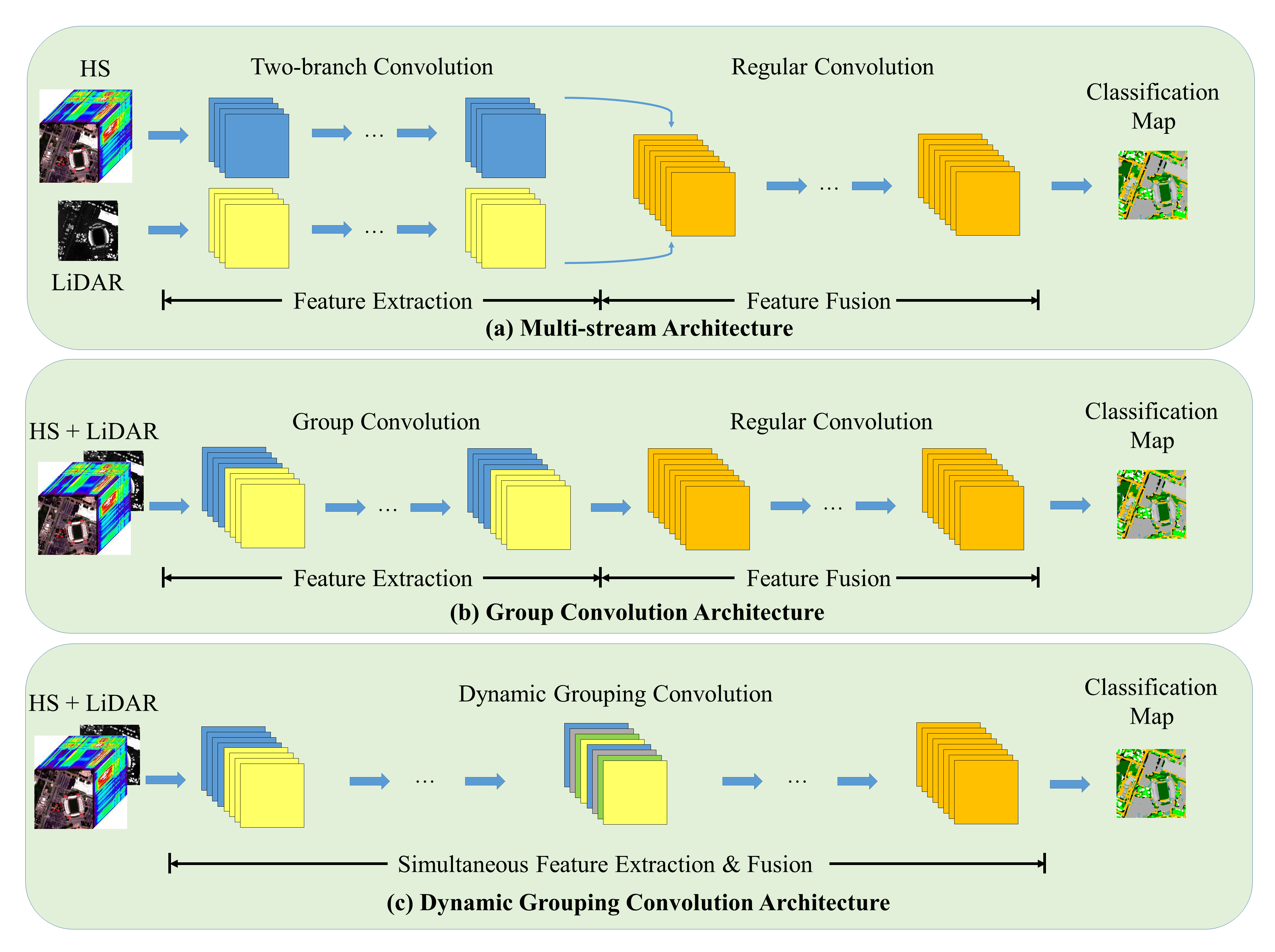
Figure 1: Illustration on the difference between (a) multi-stream architecture, (b) group convolution architecture, and (c) proposed dynamic grouping convolution architecture.

I-C Method overview

To address the aforementioned challenges, we aim in this paper to develop a framework that allows CNN architectures to be learned from data within a single-stream network, for multi-source RS data fusion.

We notice that any multi-stream architecture can be equivalently expressed by group convolution within a single-stream architecture (see Sec. II(A)). The following two parameters further control group convolution and need to be specified for each layer: number of total groups, and number of feature maps in each group. Recently proposed dynamic grouping convolution [34] (DGConv) enables these two parameters to be learned in an end-to-end manner via network training.

Originally proposed for efficient architecture designing, DGConv itself does not ensure sensor-specific features and thus cannot be directly used to approximate and study multi-stream models for multi-source RS data fusion models. In our paper, we propose necessary modifications to DGConv, based on which we further design CNN blocks and single-stream architectures with simultaneous feature extraction-fusion for joint classification of multi-source RS data. Fig. 1(c) illustrates such a CNN model. More specifically, the contributions of this paper can be highlighted as follows.

(1) A modified DGConv module, which we name SepDGConv, is proposed to automatically learn group convolution structure within single-stream neural networks. SepDGConv is theoretically compatible with any CNN architecture.

(2) Based on the proposed SepDGConv module, deep single-stream CNN models are proposed with reference to typical architectures in the CV area. The proposed CNNs show promising classification performance on various benchmark multi-source RS data sets.

(3) Experimental results suggest that using densely connected network to jointly extract features from multiple data modalities actually improves the final classification performance, and using SepDGConv in deeper layers which contain more parameters helps improve classification accuracy. This finding is very interesting since it suggests that regularization contributes more to model performance improvement than sensor-specificity.

(4) To our best knowledge, this is the first time that single-stream CNNs for multi-source RS data fusion is systematically studied and compared to state-of-the-art (SOTA) multi-branch models.

The remainder of this paper is organized as follows. The proposed DGConv layer and CNN architectures are introduced in Section II. The experimental results and analysis are presented in Section III. Finally, Section IV makes the summary with some important conclusions and hints at potential future research trends.

II PRELIMINARIES

In this section, firstly we show how we can use group convolution to construct a single-stream CNN that is equivalent to a multi-stream one. Secondly, we briefly introduce dynamic grouping convolution (DGConv) as well as G-Nets, a family of architectures using DGConv.

II-A Group conv as multi-stream conv

A CNN branch/stream consists of a sequence of convolution/normalization/activation/pooling layers, and in a multi-stream architecture, the network branches usually play the role of feature extractor. Fig. 1(a) shows a typical two-branch CNN, with HS data fed to one branch (blue) and LiDAR to the other (yellow). The output features of multi-stream feature extractors are sensor-specific, since LiDAR data is never comes into the HS branch, and vice versa. These features are further fed into a fusion sub-network, which usually consists of one single branch. The fusion sub-network makes predictions based on the extracted features and outputs classification map.

Group convolution, on the other hand, is originally proposed by the CV community for parallel computing [35]. This technique enables convolution in a layer to be computed in parallel groups. Group convolution is also studied in efficient network architecture designing [36], since it reduces the number of parameters in convolution layers. Fig. 1(b) illustrates a single-stream CNN architecture using group convolution. Input HS and LiDAR data are stacked together. In the feature extraction sub-network, the feature maps are divided into two groups in parallel, blue and yellow. HS data goes into the yellow convolution group and LiDAR data goes into the blue group. Compared to Fig. 1(a), we can see that the two architectures are identical, suppose the architecture hyperparameters, i.e., number of layers, etc., are the same.

Formally, Let $F\in\mathbf{R}^{N\times C^{in}\times H\times W}$ denote a feature map of a certain layer in a CNN, where $N,C^{in},H,W$ represent minibatch size, number of input channels, height and width of the feature map, respectively. Let $\omega\in\mathbf{R}^{C^{out}\times C^{in}\times k\times k}$ be the convolution kernel in the same layer, where $C^{out}$ is the number of output channels and $k$ is kernel size. Then in a convolution operation $F$ and $\omega$ are multiplied to give an output feature map $O\in\mathbf{R}^{N\times C^{out}\times H\times W}$:

$$O(i,j)=\sum\limits_{m=0}^{k-1}\sum\limits_{n=0}^{k-1}\omega(m,n)\,F(i+m,j+n)$$ (1)

where $i\in\{1,...,H\}$, $j\in\{1,...,W\}$, and $O(i,j)\in\mathbf{R}^{N\times C^{out}}$, $F(i+m,j+n)\in\mathbf{R}^{N\times C^{in}}$, $\omega(m,n)\in\mathbf{R}^{C^{out}\times C^{in}}$.

In regular convolution, $\omega$ densely maps every input channel to every output channel, as illustrated in Fig. 2(a). In group convolution, such dense mapping is replaced by structured mapping such that, both feature maps and convolution kernels are divided into several groups on the channel dimension, and each kernel convolves only on feature maps in the same group as the kernel. Concretely, suppose we divide the convolution into $G$ groups,

$$O^{\gamma}(i,j)=\sum\limits_{m=0}^{k-1}\sum\limits_{n=0}^{k-1}\omega^{\gamma}(m,n)\,F^{\gamma}(i+m,j+n)$$ (2)

where	$\gamma\in\{1,...,G\}$
	$\cup$ represents concatenation along the channel axis
	$O(i,j)=O^{1}(i,j)\cup...\cup O^{\gamma}(i,j)\cup...\cup O^{G}(i,j)$
	$\omega(i,j)=\omega^{1}(i,j)\cup...\cup\omega^{\gamma}(i,j)\cup...\cup\omega^{G}(i,j)$
	$F(i,j)=F^{1}(i,j)\cup...\cup F^{\gamma}(i,j)\cup...\cup F^{G}(i,j)$

Fig. 2(c) illustrates a group convolution layer with $C^{in}=C^{out}=8$ and $G=2$.

In the case of multi-source remote sensing data, if we assign one or multiple groups to each data modality, then we are able to embed multi-stream structure within a single-stream CNN. For example, suppose we have HS and LiDAR data, then we can set $G=2$, and assign HS data to group 1 and LiDAR data to group 2. Using the illustration in Fig. 2(c), let’s say HS data is on the blue colored group while LiDAR data is on the yellow colored group. Obviously this is equivalent to a two-branch network with each branch having 4 channels.

Furthermore, a common way to build deep sensor-specific branches is to set $G$ to a fixed vaule for all layers. Then in any layer, for any two different groups $\gamma_{1}$ and $\gamma_{2}$, $O^{\gamma_{1}}$ is computed only using $F^{\gamma_{1}}$, and $F^{\gamma_{2}}$ is never involved. This means that the output features are of the same sensor-specificity as the input, as the intuitive blue-to-blue, yellow-to-yellow illustration in Fig. 2(c).

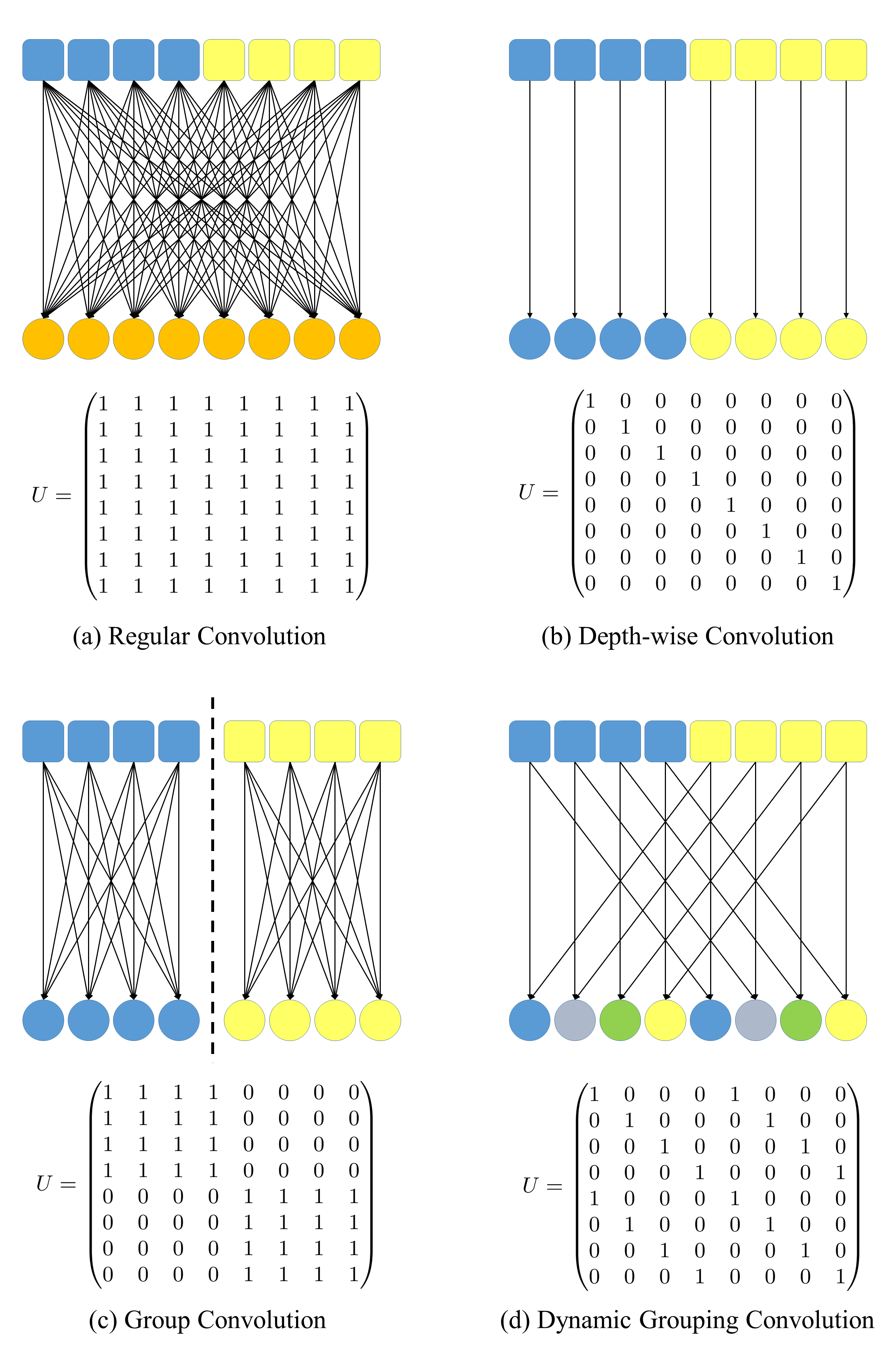
Figure 2: Illustration of different convolution strategies (above) and their corresponding relationship matrix U (below). One rectangle represents one input feature map channel, and one circle represents one output feature map channel. (a) regular convolution, (b) depth-wise convolution, (c) group convolution, and (d) dynamic grouping convolution.

Existing models using group convolution may suffer from sub-optimal performance due to manually specifying hyperparameter $G$. To address this issue, DGConv allows both the total group number and channel connections to be learned from data, alongside with other CNN parameters.

II-B Dynamic grouping convolution

Here we briefly introduce dynamic grouping convolution (DGConv) [34]. The key idea of DGConv is to model the input-output channel mapping by introducing a binary relationship matrix $U$, and then make $U$ learnable as part of the CNN parameters.

II-B1 Definition

Formally, DGConv is defined as

$$O(i,j)=\sum\limits_{m=0}^{k-1}\sum\limits_{n=0}^{k-1}(U\odot\omega(m,n))\,F(i+m,j+n)$$ (3)

where $U\in\mathbf{R}^{C^{out}\times C^{in}}$, and $\odot$ denotes element-wise product. By this definition, $U_{i}$, the $i$th row of $U$, is a binary vector that indicates which input channels are involved in the computation of the $i$th output channel.The definition is reasonable, as many convolution operations can be regarded as special cases of DGConv. For instance, DGConv becomes regular convolution (Eq. (1)) if we let $U$ be a matrix of ones, as illustrated in Fig. 2(a). DGConv becomes depth-wise convolution if we let $U$ be an identity matrix, as illustrated in Fig. 2(b). DGConv can also represent group convolution (Eq. (2)), if we take $U$ to be a block-diagonal matrix of ones and zeros, as illustrated in Fig. 2(c).

II-B2 Learning the relationship matrix U

While the definition in Eq. (3) is representative, such a definition results in the following two difficulties in estimating the value of $U$. First, the introduction of $U$ adds lots of additional parameters to the network, which makes the learning process more difficult. Second, $U$ takes binary values of 0 and 1, while it is widely known that optimization involving discrete values are generally very hard to solve.

To address the first issue, $U$ is decomposed into a set of small matrices, and learnable parameters are designed to generate this set of small matrices. Consider a simple yet quite general case, where $U$ is a square matrix with $C^{in}=C^{out}=2^{K}$, $K$ being an integer. Then a set of $2\times 2$ matrices $U_{1},...,U_{i},...,U_{K}$ can be defined, and $U$ can be reconstructed as

$$U=U_{1}\otimes...\otimes U_{i}\otimes...\otimes U_{K}$$ (4)

where $\otimes$ denotes Kronecker product, $i\in\{1,...,K\}$. Each small matrix $U_{i}$ is further represented by a binary parameter $g_{i}\in\{0,1\}$:

$$U_{i}=g_{i}\mathbf{1}+(1-g_{i})\mathit{I}$$ (5)

where $\mathbf{1}$ denotes a $2\times 2$ constant matrix of ones, $\mathit{I}$ denotes a $2\times 2$ constant identity matrix. Thus each $2^{K}\times 2^{K}$ relationship matrix $U$ can be constructed from a vector $g\in\mathbf{R}^{K}$. The number of parameters to be learned is thereby reduced exponentially.

To address the second issue, a learnable gate vector $\tilde{g}$, taking continuous values, is introduced to generate the binary vector $g$, as follows:

$$g=\text{sign}(\tilde{g})$$ (6)

where sign$(\cdot)$ represents the sign function

$$\text{sign}(x)=\left\{\begin{aligned} &0&x<0\\ &1&x\geq 0\end{aligned}\right.$$ (7)

Altogether, combining Eq. (4) - Eq. (7), the $2^{K}\times 2^{K}$ binary relationship matrix $U$ is constructed using a continuous vector $\tilde{g}$ of length $K$:

$$\begin{gathered}g=\text{sign}(\tilde{g})\\ U=g_{1}\mathbf{1}+(1-g_{1})\mathit{I}\otimes...\otimes g_{K}\mathbf{1}+(1-g_{K})\mathit{I}\end{gathered}$$ (8)

Backpropagation through the non-differentiable sign($\cdot$) can be done by Straight-Through Estimator proposed for quantized neural networks [37] , and then automatic gradient computaton for the rest is supported by most modern deep learning programming frameworks.

As an example, a convolution layer with $C^{in}=C^{out}=8$ as shown in Fig. (2) has $K=3$, and the relationship matrix $U$ is of shape $8\times 8$. $U$ for regular convolution in Fig. 2(a) can be expressed as $U=\mathbf{1}\otimes\mathbf{1}\otimes\mathbf{1}$, with $g=(1,1,1)$. Similarly, for depth-wise convolution in Fig. 2(b), $g=(0,0,0)$ and $U=\mathit{I}\otimes\mathit{I}\otimes\mathit{I}$. For group convolution illustrated as Fig. 2(c), $g=(1,1,0)$ and $U=\mathbf{1}\otimes\mathbf{1}\otimes\mathit{I}$. For DGConv shown in Fig. 2(d), $g=(0,0,1)$ and $U=\mathit{I}\otimes\mathit{I}\otimes\mathbf{1}$.

II-C G-Nets

Groupable-Networks (G-Nets) [34] refer to architectures using DGConv. In particular, the authors of [34] experiment with G-ResNet50, which is based on ResNet50 [38].

ResNet50 uses Bottleneck as its building block. The Bottleneck block in order consists of one $1\times 1$ convolution layer, one $3\times 3$ convolution layer, and one more $1\times 1$ convolution layer, as shown in Fig. 3(c). In its DGConv version, the middle $3\times 3$ convolution is replaced with $3\times 3$ DGConv. G-ResNet50 consists of four Bottleneck blocks, the number of output channels for each block being $[256,512,1024,2048]$, respectively.

III METHOD

While DGConv enables automatically learning of group convolution hyperparameters, the learning outcome does not lead to a network with sensor-specific branches, as we will see below, and thus cannot be directly used to approximate multi-branch CNNs for multi-source RS data fusion. To address this issue, based on DGConv we propose separable DGConv (SepDGConv) and separable G-Net (SepG-Net), which makes it possible that the learned architecture contains sensor-specific branches.

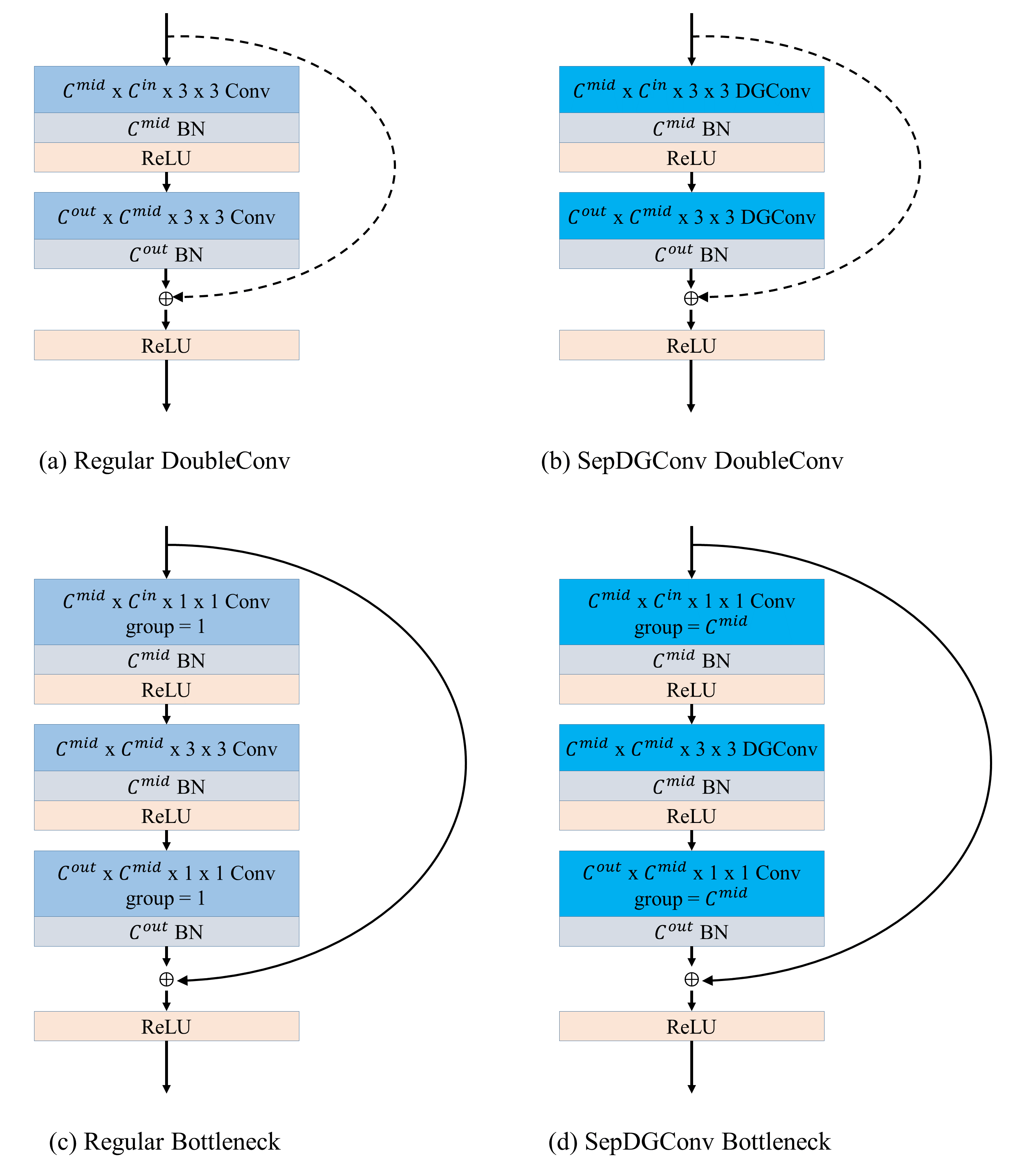
Figure 3: CNN blocks and their corresponding SepDGConv variant. (a) regular DoubleConv, (b) SepDGConv DoubleConv , (c) regular Bottleneck, and (d) SepDGConv Bottleneck. The curve with arrow stands for residual connection in ResNet blocks, and $\oplus$ denotes summation. In (a) and (b), the dashed curve means there is no residual connection when DoubleConv is used in UNet.

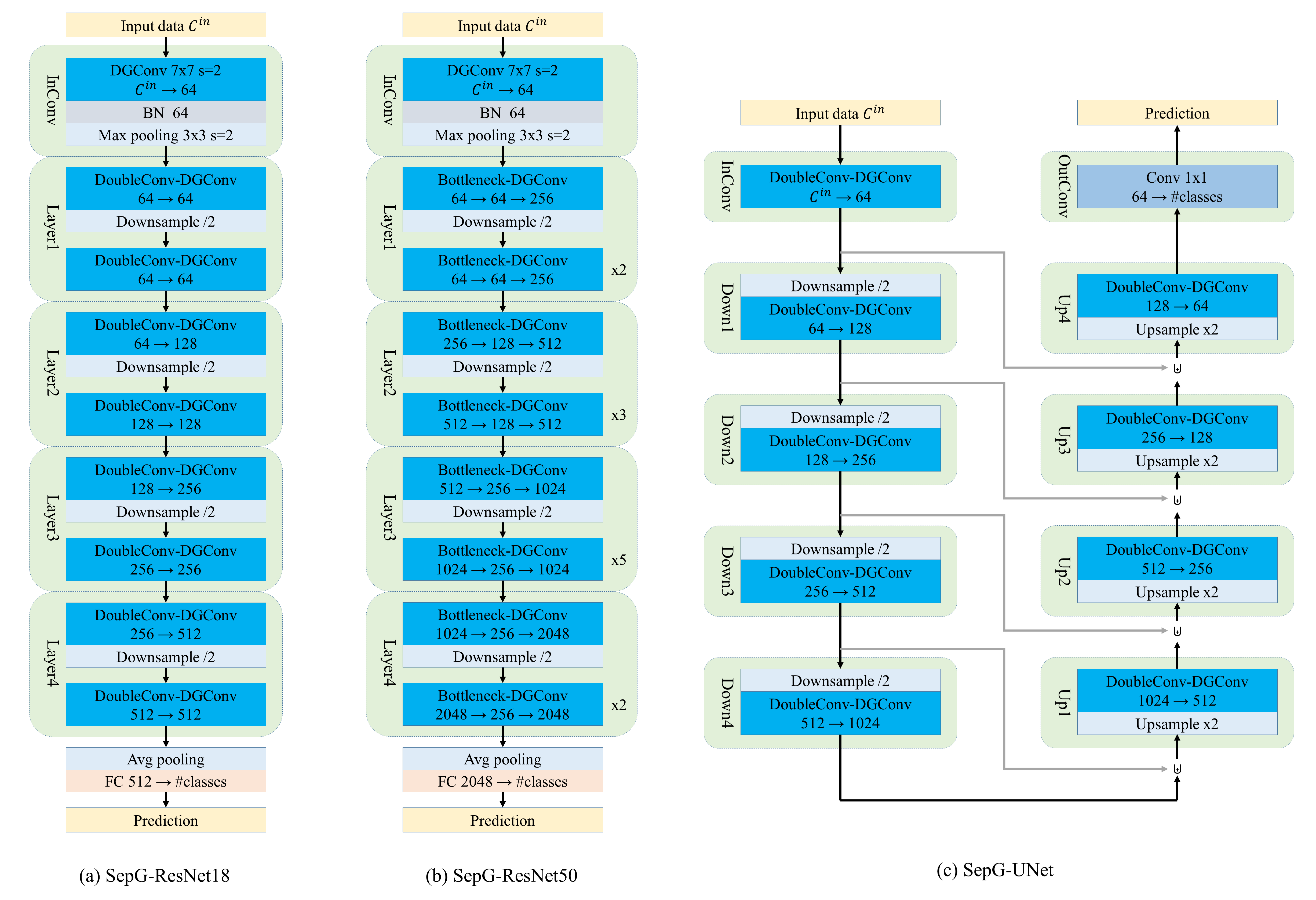
Figure 4: Neural network architectures using SepDGConv. (a) SepG-ResNet18, (b) SepG-ResNet50, and (c) SepG-UNet. In (b), the $\times x$ means that $x$ consecutive blocks are omitted as one in the illustration. In (c), grey line represents skip connections utilized in UNet, while $\uplus$ denotes concatenation along the channel axis.

III-A Blocks with SepDGConv

First, reconsider the Bottleneck block with DGConv. If sensor-specificity is to be preserved, then it is necessary that every convolution layer in a block uses group convolution, as in Eqn. (2). In both regular and DGConv Bottleneck blocks, the first and last convolution layer use $1\times 1$ regular convolution. Therefore, in our SepDGConv Bottleneck, we use depth-wise convolution instead of regular convolution, i.e., we set the number of groups $G$ equal to the number of that layer’s feature maps. Fig. 3(d) shows a SepDGConv Bottleneck block.

Second, consider the DoubleConv block, which is used as building blocks by two very popular CNN models: ResNet18 and UNet [39]. A DoubleConv block consists of two consecutive $3\times 3$ convolution layers, as shown in Fig. 3(a). For the ResNet family, BasicBlock has a very similar structure to that of DoubleConv, except for the additional residual connection of BasicBlock. As long as there is no confusion, we also use DoubleConv to refer to BasicBlock in ResNets. To impose sensor-specificity, in our SepDGConv DoubleConv, we replace both convolution layers with DGConv layers, as shown in Fig. 3(b).

III-B Details of SepDGConv

Recall that in section II(B), for DGConv it is assumed on the relationship matrix $U\in\mathbf{R}^{C^{out}\times C^{in}}$ that $C^{out}=C^{in}=2^{K}$. To apply DGConv to all layers in order to approximate deep sensor-specific branches, in our SepDGConv we handle the following two exceptions that violate the above assumption.

III-B1 $C^{out}\neq C^{in}$

For architectures mentioned above, Bottleneck by our design satisfies this condition, however DoubleConv usually has $C^{out}\neq C^{in}$. $C^{out}>C^{in}$ is commonly seen in the feature extraction phase of a CNN, where the latter layer has more feature maps than its previous layer. $C^{out}<C^{in}$ is often used in upsampling layers of a segmentation model.

Formally we define the following case expansion: $C^{out}/C^{in}=r$, and the other case reduction: $C^{in}/C^{out}=r$, with $r\geq 2$ being an integer. Our strategy is to expand or reduce the shape of the relationship matrix by doing matrix multiplication and Kronecker product with identity matrices and vectors of ones.

In the expansion case, we first construct a matrix $\tilde{U}\in\mathbf{R}^{C^{in}\times C^{in}}$ as described in subsection II(B). Recall that $U(i,j)=1$ if the $j$th input channel is involved in the computation of the $i$th output channel, otherwise $U(i,j)=0$. Hence we duplicate each row of $\tilde{U}$ $r$ times, and stack them together horizontally to get $U$:

$$U=(I\otimes\mathbf{1}_{r})\tilde{U}$$ (9)

where $I$ is a ${C^{in}\times C^{in}}$ identity matrix, and $\mathbf{1}_{r}$ is a column vector of ones, with length $r$.

Similarly, in the reduction case, we first construct $\tilde{U}\in\mathbf{R}^{C^{out}\times C^{out}}$. Then we duplicate each column of $\tilde{U}$ $r$ times, and stack them together vertically:

$$U=\tilde{U}(I\otimes\mathbf{1}^{\top}_{r})$$ (10)

where $I$ is a ${C^{out}\times C^{out}}$ identity matrix, and $\mathbf{1}^{\top}_{r}$ is a row vector of ones, with length $r$.

With our proposed strategy we encourage feature maps in one input group to stay in the same output group. Also, note that both $(I\otimes\mathbf{1}_{r})$ and $(I\otimes\mathbf{1}^{\top}_{r})$ are fixed during network initialization phase and need no training.

III-B2 $C^{in}\neq 2^{K}$

Finally we present how we handle $C^{in}\neq 2^{K}$, which is commonly seen in the input convolution block (InConv) of a CNN that computes convolution on the input data.

For remote sensing data, the number of input data channels can range from $\sim 3$ (RGB data) to $\sim 10^{2}$ (HS data), while very commonly the number of input channels for the first block after InConv is set to $64$, which means for InConv $C^{out}=64$. Hence $C^{in}$ for InConv can fall within any of the following 3 intervals: $(0,\frac{1}{2}C^{out})$, $(\frac{1}{2}C^{out},2C^{out})$, $(2C^{out},+\infty)$.

If $0<C^{in}<\frac{1}{2}C^{out}$, then we hope to use Eqn(9) to construct $U$. We make the following modification to make sure both $K$ and $r$ are integers:

$$\begin{gathered}K=\lceil\text{log}_{2}(C^{in})\rceil\\ r=\lceil C^{out}/C^{in}\rceil\end{gathered}$$ (11)

where $\lceil x\rceil$ denotes the round up function.

Similarly, we use Eqn(10) for $2C^{out}<C^{in}<+\infty$, with

$$\begin{gathered}K=\lceil\text{log}_{2}(C^{out})\rceil\\ r=\lceil C^{in}/C^{out}\rceil\end{gathered}$$ (12)

For the last case $\frac{1}{2}C^{out}<C^{in}<2C^{out}$, we determine $K$ and round it up to an integer:

$$K=\lceil\text{log}_{2}(\text{max}(C^{in},C^{out}))\rceil$$ (13)

where $\text{max}(a,b)$ takes the maximum of $a$ and $b$.

Finally, the size of $U$ constructed by our design is always larger than $\mathbf{R}^{C^{out}\times C^{in}}$. Hence we only use the first $C^{out}$ rows and $C^{in}$ columns in our computation, ignoring the remaining entries.

III-C SepG-Nets

Using SepDGConv DoubleConv, we can build SepG-ResNet18, as shown in Fig. 4(a), and SepG-UNet, as shown in Fig. 4(c). In SepG-ResNet18, we follow the convention and build the network with four layers, each having 2 DoubleConv blocks. The number of output channels for each layer being $[64,128,256,512]$, respectively. In SepG-UNet, we have 8 DoubleConv blocks, with output channel numbers $[128,256,512,1024,512,256,128,64]$.

SepG-ResNet50 consists of four layers, in order composed of $[2,3,5,2]$ SepDGConv Bottleneck blocks. The number of output channels for each block is the same as G-ResNet50, being $[256,512,1024,2048]$ respectively. The architecture of SepG-ResNet50 is illustrated in Fig. 4(b).

IV EXPERIMENTS AND DISCUSSION

We experiment with SepG-ResNet18, SepG-ResNet50 and SepG-UNet on three diverse data sets: Houston2018 data set, Berlin data set and MUUFL data set, and compare with baseline models, as well as SOTA models on the data sets. In this section, firstly we describe the data sets. Secondly we present our experimental results. Thridly, we analyze the role of SepDGConv in the entire model by ablation analysis and we report changes in classification performance. Fourthly, we compare different convolution strategies, in particular group convolution and SepDGConv, to isolate the effect of sensor-specificity. Finally, we discuss the results and findings of our experiments.

IV-A Data sets

IV-A1 Houston2018 data set

Houston2018 is an HS-LiDAR-RGB data set. Acuqired by the National Center for Airborne Laser Mapping at the University of Houston, the Houston2018 data set covers the University of Houston campus and its surrounding urban areas. The data set consists of MS-LiDAR, HS, and MS-optical remote sensing data, each containing 7, 48, and 3 channels, respectively. The HS data covers a 380–1050 nm spectral range, while laser wavelengths of 3 LiDAR sensors are 1550, 1064 and 532 nm. The MS-LiDAR data also contains DEM and DSM derived from point clouds. This data set was originally provided in 2018 GRSS Data Fusion Contest. This paper [3] reports the outcome of the Contest, and also contains more detailed description of the Houston2018 data set. We resample the imagery at a 0.5-m GSD, so that the size of each image channel is $2404\times 8344$ pixels. The ground truth of data set contains 20 classes. The number of samples in each class are shown in Table I.

TABLE I: LULC classes in Houston2018 data set

#	Class	# Training samples	# Test samples
1	Healthy Grass	39196	20000
2	Stressed Grass	130008	20000
3	Artificial Turf	2736	20000
4	Evergreen Trees	54322	20000
5	Deciduous Trees	20172	20000
6	Bare Earth	18064	20000
7	Water	1064	1628
9	Non-residential Buildings	894769	20000
10	Roads	183283	20000
11	Sidewalks	136035	20000
12	Crosswalks	6059	5345
13	Major Thoroughfares	185438	20000
14	Highways	39348	20000
15	Railways	27748	11232
16	Paved Parking Lots	45932	20000
17	Unpaved Parking Lots	587	3524
18	Cars	26289	20000
19	Trains	21479	20000
20	Stadium Seats	27296	20000
	Total	1859825	321729

IV-A2 Berlin data set

This is an HS-SAR data set. The Berlin data set covers the Berlin urban and its rural neighboring area. The data set consists of HS and MS-SAR imagery, containing 244 and 4 channels respectively. The HS data was originally provided by [40], with wavelength range of 400 nm to 2500 nm, while more recently the authors of [41] acquired MS-SAR data of the same area and processed both HS and MS-SAR data into analysis- ready form, which is used in our experiments. The processed data has a 13.89m GSD and consists of $1723\times 476$ pixels. The Berlin data set contains 15 classes of ground truth labels. The number of samples in each class are shown in Table II.

TABLE II: LULC classes in Berlin data set

#	Class	# Training samples	# Test samples
1	Forest	443	54511
2	Residential Area	423	268219
3	Industrial Area	499	19067
4	Low Plants	376	58906
5	Soil	331	17095
6	Allotment	280	13025
7	Commercial Area	298	24526
8	Water	170	6502
	total	2820	461851

IV-A3 MUUFL Data Set

The MUUFL Gulfport data set [42] is an HS-LiDAR data set. It was collected over the University of Southern Mississippi Gulf Park Campus. The data set contains coregistered HS and MS-LiDAR data, with 64 and 2 bands respectively. The wavelength of HS data spectral bands ranges from 375 to 1050 nm. The data set contains $325\times 220$ pixels, with spatial resolution of 0.54 m across track and 1.0 m along track. In the ground truth labels there are 11 classes. The number of samples in each class are shown in Table III.

TABLE III: LULC classes in MUUFL data set

#	Class	# Training samples	# Test samples
1	Trees	100	23246
2	Mostly Grass	100	4270
3	Mixed Ground Surface	100	6882
4	Dirt and Sand	100	1826
5	Road	100	6687
6	Water	100	466
7	Building Shadow	100	2233
8	Building	100	6240
9	Sidewalk	100	1385
10	Yellow Curb	100	183
11	Cloth Panels	100	269
	Total	1100	53687

IV-B Classification and results

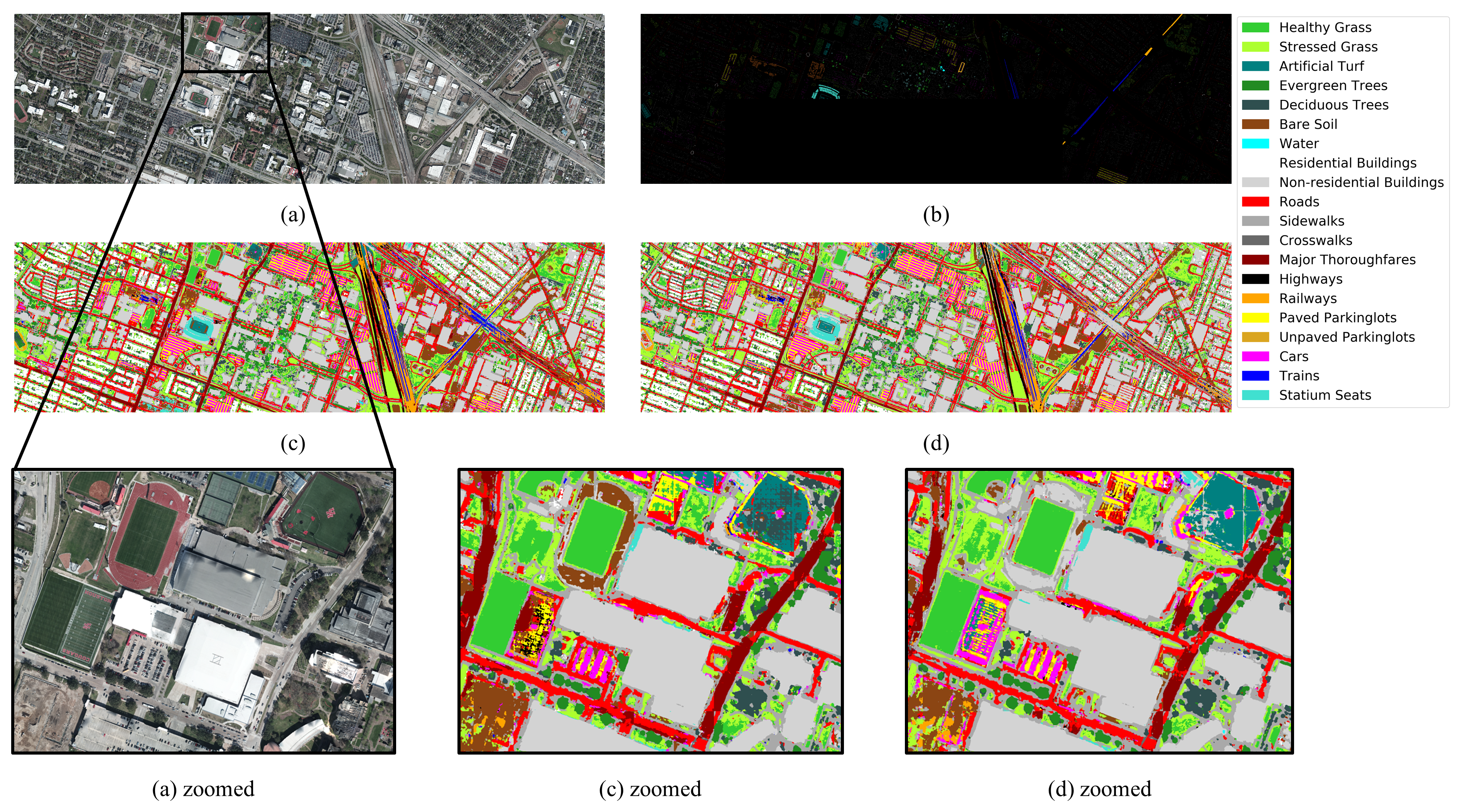
Figure 5: Results on Houston2018 data set. (a) MS optical image, (b) test ground truth labels, (c) prediction map by ResNet18, and (d) prediction map by SepG-ResNet18. Zoomed in image from (a), (c) and (d) are shown in the bottom row.

Since the data modality of the above 3 data sets are quite different from each other, we use different classification models and compare with different methods on each data set. We will present data preparation, experimental settings and classification results seperately for each data set. Here we state some global configurations in our experiments.

Environment and reproducibility We run our models on NVIDIA GTX 1080 Ti GPUs throughout our experiments. Software we use include: CUDA 10.2, cuDNN 7.6.5, python 3.8.2, pytorch 1.9.0, torchvision 0.10.0, scipy 1.6.2, and numpy 1.20.2. In all our experiments we run 5 replicas for each model using random seeds 42-46. The reproducibility of our experimental results depends on random seeds, software, and hardware. Note that using deterministic algorithms to a certain extent reduces classification accuracy of our models.

Preprocessing For all the data utilized in our experiments, we use channel-wise normalize to rescale each channel into the range $[0,1]$:

$$channel[i,j]=\frac{channel[i,j]-\text{min}(channel)}{\text{max}(channel)-\text{min}(channel)}$$ (14)

where $channel$ is a 2D array representing one image channel, $\text{max}(channel)$ and $\text{min}(channel)$ takes the maximum and minimum value from $channel$, respectively.

For more details of data preparation we follow previous work unless otherwise specified. For Houston2018 data set, we follow [24]. For Berlin data set, we follow [41]. For MUUFL data set, we follow [28].

Initialization If not specified, we draw initial values from the uniform distribution, which is also the default initialization method in Pytorch.

Optimization Since there are varying degrees of data imbalance in all the three data sets, we use the weighted cross entropy loss to train CNN models, with weight for each class set to

$$w_{c}=1-\frac{\#samples_{c}}{\#total\_samples}$$ (15)

where $w_{c}$ denotes class weight for class $c$, $\#samples_{c}$ represents number of training samples of class $c$, and $\#total\_samples$ represents the total number of samples in the training set.

Metrics To evaluate the classification results, for each classifier we will report F1-score (F1) for each class, and three widely-used criteria in the literature to evaluate overall performance, i.e., average accuracy (AA), overall accuracy (OA) and Kappa coefficient ($\kappa$).

IV-B1 Experiments on Houston2018 data set

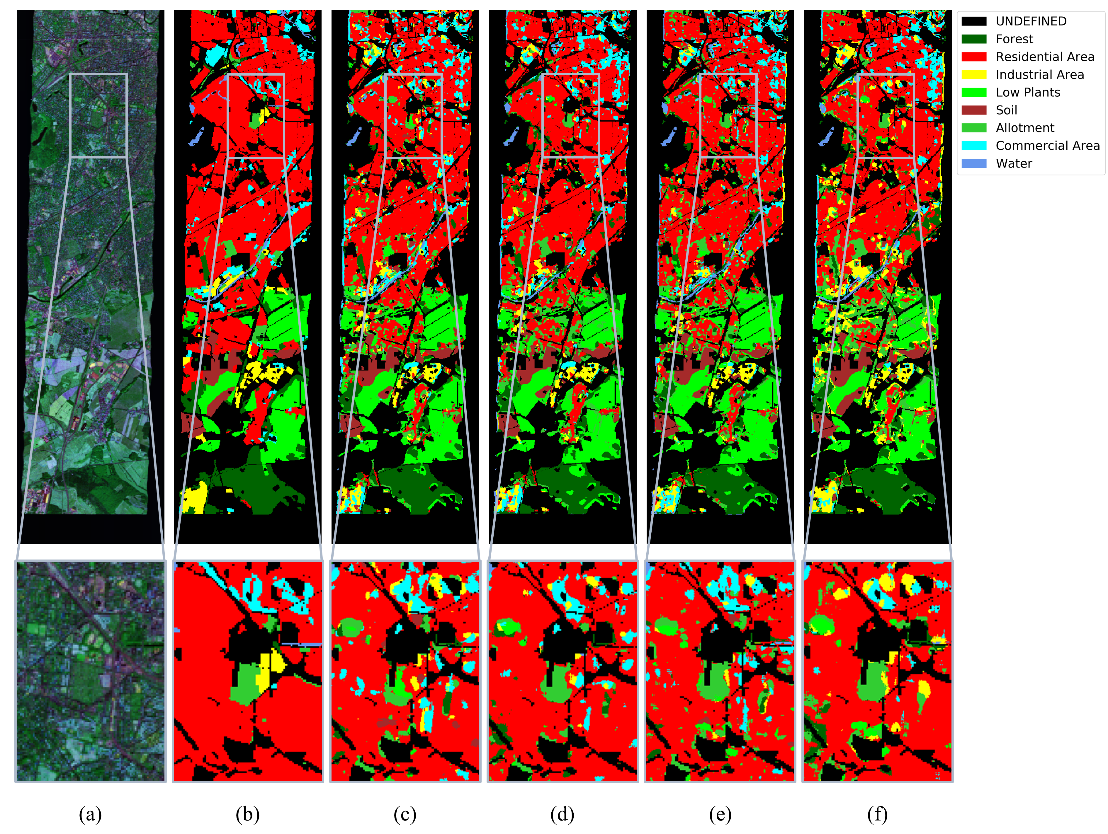
Figure 6: Results on Berlin data set. (a) HS false color image, (b) test ground truth labels, and prediction maps by (c) ResNet18, (d) SepG-ResNet18, (e) ResNet50, and (f) SepG-ResNet50.

We follow [24] and treat the LULC classification on Houston2018 data set as a semantic segmentation problem, and experiment with UNet, a very commonly studied semantic segmentation model. We run basic UNet on the data set as a baseline, and examine the performance of SepG-UNet, where SepDGConv layers replace regular convolution layers in the baseline model. We also compare with the first and second place methods presented in 2018 Data Fusion Contest, both are multi-stream models: Fusion-FCN [24] and DCNN [43].

Implementation details We use Image tiles of shape $58\times 128\times 128$. In the training phase we use a spatial stride of $64\times 64$ pixels to extract training samples from the $58\times 1202\times 4768$ data, while in the test phase the stride is $128\times 128$.

We use the Adam optimizer [44] to train both UNet and SepG-UNet, with optimizer hyperparameters $\beta_{1}$ and $\beta_{2}$ set to default values. We set the initial learning rate to 0.001, and train the networks for 300 epochs. We use 3 GPUs in parallel to train the networks, with batch size set to 12. To ensure reproducibility we use transpose convolution in upsampling modules in UNet and SepG-UNet. While the reference data for Houston2018 data set is densely labeled, there are still some areas on the image where there are no annotations. We add a mask to the loss function so that these undefined pixels are not accounted for training loss.

Results The quantitative classification results of SepG-UNet, UNet, Fusion-FCN and DCNN are shown in Table IV, while Fig. 5(c) and 5(d) shows the classification map of UNet and SepG-UNet, alongside with the ground truth labels. In Table IV, the classification results of DCNN and Fusion-FCN are directly cited from [3]. Note that, in [3] ensembling is used and the authors actually report the performance of an ensemble of Fusion-FCN. Our experimental results show that basic UNet, which does not has a multi-stream architecture, can yield an overall accuracy of $63.66\%$, outperforming $63.28\%$ obtained by ensembled Fusion-FCN, and largely outperforming DCNN. And with the proposed SepDGConv, the performance of SepG-UNet is further improved to $63.66\%$. From Fig. 5, it can be seen that both UNet and SepG-UNet can output meaningful prediction maps. According to Table IV, using SepDGConv reduces OA variance, which is reflected in Fig. 5(c) and Fig. 5(d) that SepG-UNet gives a generally less noisy classification map than basic UNet.

In Fig. 8(a), we plot the learned number of groups and sparsity of relationship matrix $U$ for each SepDGConv layer in SepG-UNet. Here the sparsity of $U$ is defined as the ratio between number of 0s and number of total entries in $U$. The Sparsity plot shows that SepDGConv generates an architecture with dense-sparse connection alternately appearing. While in InConv block the learned $U$s are mostly sparse, the sparsities quickly drop to 0 in Down1 block in all 5 replicas, which suggests that sensor-specific branches learned in SepG-UNet are very shallow, and feature fusion probably begins in a very early stage. In the #Groups plot, we can see that SepDGConv learns more groups in middle layers where there are more feature maps and more parameters. This is consistent with the behaviour of DGConv found in the paper [34].

IV-B2 Experiments on Berlin data set

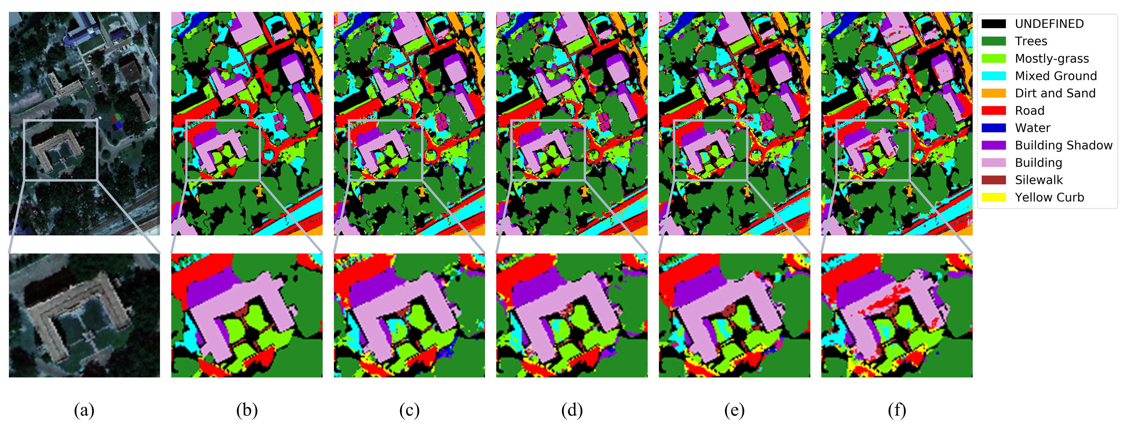
Figure 7: Results on MUUFL data set. (a) HS false color image, (b) test ground truth labels, and prediction maps by (c) ResNet18, (d) SepG-ResNet18, (e) ResNet50, (f) SepG-ResNet50.

In Berlin data set, the ground truth labels are sparse, so we extract small image patches as training and testing samples, with the center of each image patch aligned with one label. Hence LULC classification on Berlin data set becomes a image classification task. We select ResNet18 and ResNet50 as baseline, and experiment with SepG-ResNet18 and SepG-ResNet50, where regular convolution layers in the baseline models are replaced with SepDGConv layers. In addition, we compare with S2FL[41], which achieves SOTA performance on this data set.

Implementation details For SepG-ResNet18, ResNet18, SepG-ResNet50 and ResNet50, we use image patch of $17\times 17$ as training and test samples.

To train SepG-ResNet18 and ResNet18 we use stochastic gradient descent with momentum as our optimizer, with momentum parameter set to 0.9. We train the networks for 300 epochs. Initial learning rate is set to 0.001. Both models are trained on a single GPU using a batch size of 64. For SepG-ResNet50 and ResNet50, we use Adam as optimizer, with default algorithm parameters. We train both networks for 400 epochs. Initial learning rate is set to 0.001, which is further decayed to 0.0001 at the 300th epoch. Both models are trained on a single GPU using a batch size of 64.

Results The quantitative classification results of SepG-ResNet18, ResNet18, SepG-ResNet50, ResNet50 and S2FL are shown in Table V, while Fig. 6 shows the classification map of our models, alongside with the ground truth labels. In Table V, we directly cite the results of S2FL from [41]. While S2FL is not DL-based, it is essentially multi-stream and achieves SOTA performance on Berlin data set so we believe it is worthy of reference. Our experimental results show that ResNet based methods generally outperform S2FL. SepG-ResNet18 surpasses its baseline model and improves SOTA OA on Berlin data set to $68.21\%$, while SepG-ResNet50 obtains a marginally lower classification accuracy than basic ResNet50. We will see in Sec. IV(C) that the best performance is achieved using the ResNet50 architecture when some but not all convolution layers are replaced with SepDGConv. Variance reduction is also observed on SepDGConv models. Fig. 6 shares a similar visual comparison with quantitative results.

SepDGConv group structure plots for SepG-ResNet18 and SepG-ResNet50 are shown in Fig. 8(b) and 8(c). The Sparsity plot shows that both learned architectures are generally sparse, however sparsity drop in shallow layers, which suggests early fusion, is also found present in SepG-ResNet18 and SepG-ResNet50 on Berlin data set. The #Groups plot shows that, in SepG-ResNet18, InConv learns $\sim 10$ groups, while in SepG-ResNet50, InConv learns $2-4$ groups, which is in contrary to the empirical principle that the number of groups should be the same as the number of sensors. Besides, there are generally more groups in the last two blocks than in previous blocks for both models. Since in ResNets there are more feature maps and thus more parameters in Layer3 and Layer4, this result is also consistent with SepG-UNet.

TABLE IV: Model performance on Houston2018 data set

#	Class	Performance (%)
		DCNN	Fusion-FCN	UNet	SepG-UNet
1	Healthy Grass	99.2	88.70	83.67±1.47	82.68±2.61
2	Stressed Grass	0.0	87.30	67.17±2.65	69.11±2.43
3	Artificial Turf	21.3	64.14	39.85±17.13	56.46±22.66
4	Evergreen Trees	95.6	97.05	82.20±2.15	84.00±1.31
5	Deciduous Trees	59.7	73.02	63.25±4.41	67.78±7.57
6	Bare Earth	5.4	27.64	52.05±4.43	48.05±4.51
7	Water	96.7	9.15	24.43±20.68	16.83±1.51
8	Residential Buildings	0.0	75.03	71.72±4.66	70.50±4.62
9	Non-residential Buildings	95.1	93.55	64.73±2.63	61.87±1.63
10	Roads	76.0	62.44	52.25±1.79	52.13±3.25
11	Sidewalks	69.5	68.52	62.68±3.33	63.56±4.12
12	Crosswalks	0.0	7.46	26.35±4.35	38.02±13.80
13	Major Thoroughfares	33.3	59.94	35.38±0.81	31.53±0.70
14	Highways	30.3	17.95	43.94±6.26	33.16±4.79
15	Railways	85.4	80.46	36.23±14.58	48.44±10.28
16	Paved Parking Lots	58.4	60.80	71.44±3.46	72.55±8.09
17	Unpaved Parking Lots	0.0	0.00	0.00±0.00	0.00±0.00
18	Cars	0.0	64.33	71.45±2.36	74.87±3.96
19	Trains	89.6	50.94	92.44±1.36	88.30±5.93
20	Stadium Seats	85.1	41.97	75.46±9.16	71.06±8.49
AA		50.0	56.52	55.84±5.38	56.55±5.61
OA		51.2	63.28	63.66±1.39	63.74±1.05
Kappa		0.48	0.61	0.61±0.01	0.62±0.01

TABLE V: Model performance on Berlin data set

#	Class	Performance (%)
		S2FL	ResNet18	SepG-ResNet18	ResNet50	SepG-ResNet50
1	Forest	83.30	61.03±7.67	68.25±2.59	63.74±3.35	65.73±3.87
2	Residential Area	57.39	76.92±4.26	79.85±2.52	78.73±3.16	78.28±1.16
3	Industrial Area	48.53	37.43±2.47	39.26±3.06	38.78±3.11	34.65±3.40
4	Low Plants	77.16	75.57±2.75	74.70±1.63	75.85±1.64	73.62±3.02
5	Soil	83.84	69.60±3.91	68.26±4.68	66.02±3.10	68.63±7.56
6	Allotment	57.05	19.64±2.56	25.47±2.16	23.21±2.07	27.51±4.32
7	Commercial Area	31.02	27.52±1.03	25.02±3.33	31.60±3.68	26.89±3.07
8	Water	61.57	60.04±1.73	53.05±1.95	58.05±5.47	57.71±8.17
AA		62.23	53.47±3.30	54.23±2.74	54.49±3.20	54.13±4.32
OA		62.48	65.43±3.56	68.21±2.43	66.98±2.73	66.32±0.72
Kappa		0.49	0.51±0.04	0.54±0.03	0.53±0.03	0.53±0.01

TABLE VI: Model performance on MUUFL data set

#	Class	Performance (%)
		OTVCA	TB-CNN	ResNet18	SepG-ResNet18	ResNet50	SepG-ResNet50
1	Trees	84.74±7.28	89.97±1.12	93.33±0.43	92.13±1.11	92.23±1.68	91.81±0.47
2	Mostly Grass	82.47±0.71	80.61±4.98	72.76±1.74	71.82±1.91	71.96±3.95	72.90±2.72
3	Mixed Ground Surface	69.93±1.40	73.25±8.15	75.91±1.18	74.56±1.60	73.71±1.55	73.55±1.89
4	Dirt and Sand	85.93±0.62	83.46±1.48	85.16±1.11	85.73±1.54	83.95±1.60	83.88±1.22
5	Road	83.76±2.84	88.04±0.48	90.25±0.75	87.93±2.12	86.9±1.09	83.33±1.57
6	Water	99.45±1.14	67.60±0.13	73.74±6.60	76.23±7.62	74.73±4.94	78.73±6.07
7	Building Shadow	91.19±0.61	84.55±3.01	79.25±2.19	75.73±3.30	82.33±1.78	80.61±2.77
8	Building	96.66±5.85	92.92±0.81	95.26±0.41	91.39±3.17	94.11±0.66	88.94±0.74
9	Sidewalk	75.80±0.39	67.73±4.46	65.78±2.24	63.40±3.15	54.17±2.79	56.68±3.00
10	Yellow Curb	89.16±0.33	17.49±2.71	31.10±4.13	30.80±6.28	22.54±2.94	24.14±3.16
11	Cloth Panels	98.22±0.31	43.12±0.41	83.17±4.67	82.97±2.78	70.69±6.19	65.62±7.58
AA		84.15±0.56	85.47±1.05	76.88±2.31	75.70±3.14	73.39±2.65	72.75±2.84
OA		79.57±2.00	84.47±1.27	86.44±0.11	84.6±1.85	84.28±1.28	83.23±0.65
Kappa		0.87±0.01	0.72±0.02	0.83±0.00	0.80±0.02	0.80±0.02	0.79±0.01

IV-B3 Experiments on MUUFL data set

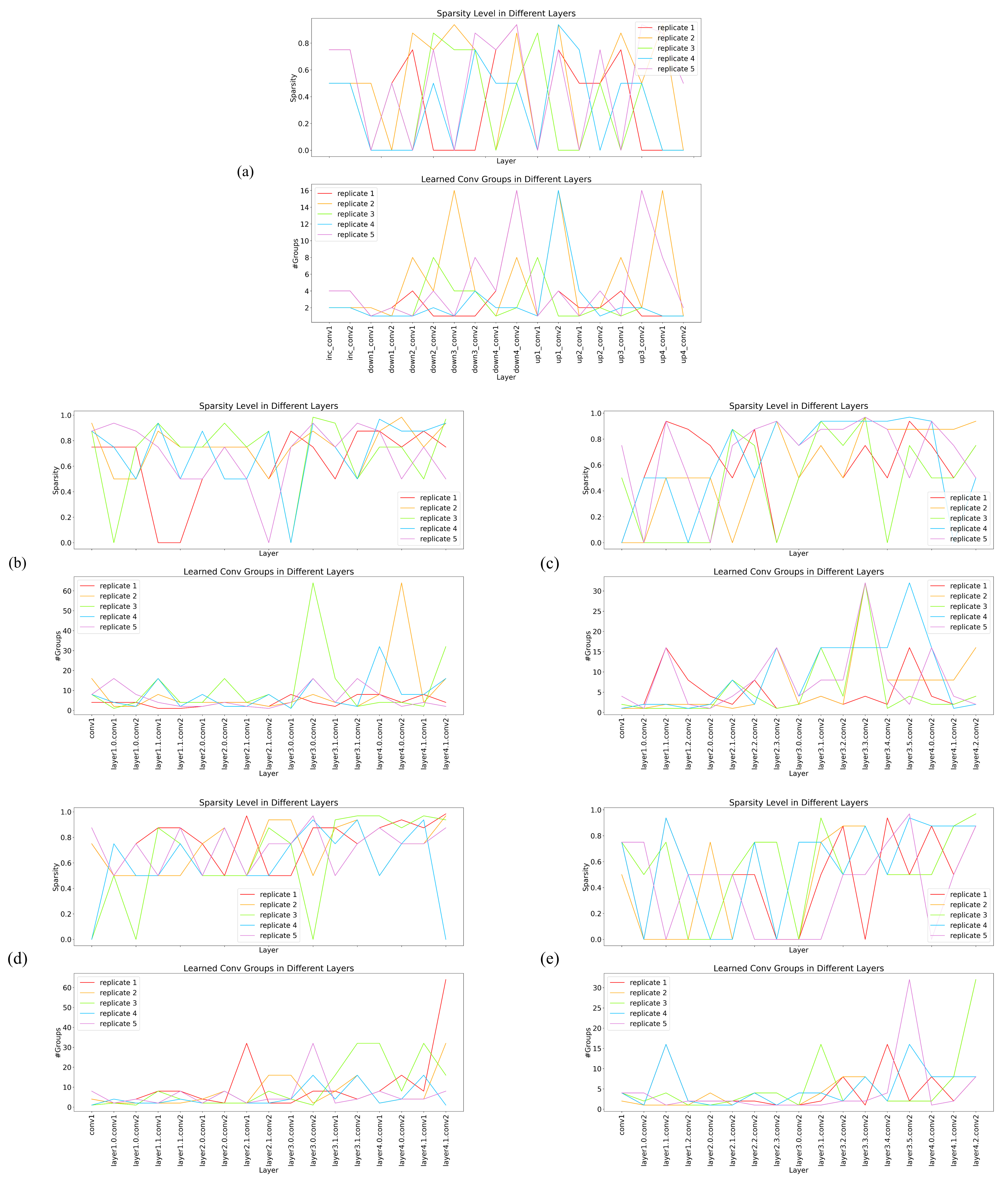
Figure 8: Number of groups and sparsity of U in each layer of the following SepDGConv-based models on different data sets: (a) SepG-UNet trained on Houston2018 data set, (b) SepG-ResNet18 trained on Berlin data set, (c) SepG-ResNet50 trained on Berlin data set, (d) SepG-ResNet18 trained on MUUFL data set, and (e) SepG-ResNet50 trained on MUUFL data set,

For MUUFL data set we follow most studies on it and use classification models. We experiment with ResNet18, ResNet50 and their Sep-DGConv derivatives on MUUFL data set. We also compare our results with those of the following methods: orthogonal total variation component analysis (OTVCA) [6], and two branch CNN (TB-CNN) [23]. Both OTVCA and TB-CNN are multi-stream models.

Implementation details For SepG-ResNet18 and ResNet18, we use image patch of $11\times 11$ as training and test samples, while for SepG-ResNet50 and ResNet50, we use image patch of size $17\times 17$. Since previous studies do not use a fixed training set, we make random train-test split in each replica under different random seeds. We follow [28] and set training set size fixed to 100 and the rest used as test set.

For SepG-ResNet18 and ResNet18, we use He initialization [45] to initialize convolution filters, and zero initialization for the last batch normalization layer in each residual branch [46]. To train the networks we use stochastic gradient descent with momentum as our optimizer, with momentum parameter set to 0.9. We train the networks for 300 epochs. Initial learning rate is set to 0.02, with a learning rate schedule that decreases the learning rate to 0.002 at 200th epoch, and further decreases the learning rate to 0.0002 at 240th epoch. Both models are trained on a single GPU using a batch size of 48. In SepG-ResNet50 and ResNet50, He initialization and zero batch norm initialization are also used. We use Adam as optimizer, with default algorithm parameters. We train both networks for 400 epochs. Initial learning rate is set to 0.01, with a learning rate schedule at epochs [300, 350], decreasing the learning rate to [0.001, 0.0001]. Both models are trained on a single GPU using a batch size of 64.

Results The quantitative classification results of SepG-ResNet18, SepG-ResNet50, ResNet18, ResNet50, and methods to compare with are shown in Table VI. These results are cited from [28] who replicated these models in their work, since we follow their experimental settings. Fig. 7 shows the classification map of these models alongside with the ground truth labels. According to Table VI, the ResNets generally achieve better performance than OTVCA and TB-CNN. On MUUFL data set, however, both SepG-ResNet18 and SepG-ResNet50 do not surpass their corresponding baseline model. Again we will see in Sec. IV(C) that by using SepDGConv in some but not all convolution layers both models can obtain better performance and outperform baseline models. In Fig. 7, the output classification maps of ResNet50s are generally more noisy than those of ResNet18s, which suggest that there is probably overfitting in ResNet50s, since the data set is relatively small.

SepDGConv group structures learned on MUUFL data set are shown in Fig. 8(d) and 8(e). Both early fusion and more groups in deeper layers are consistently observed.

IV-C Ablation analysis

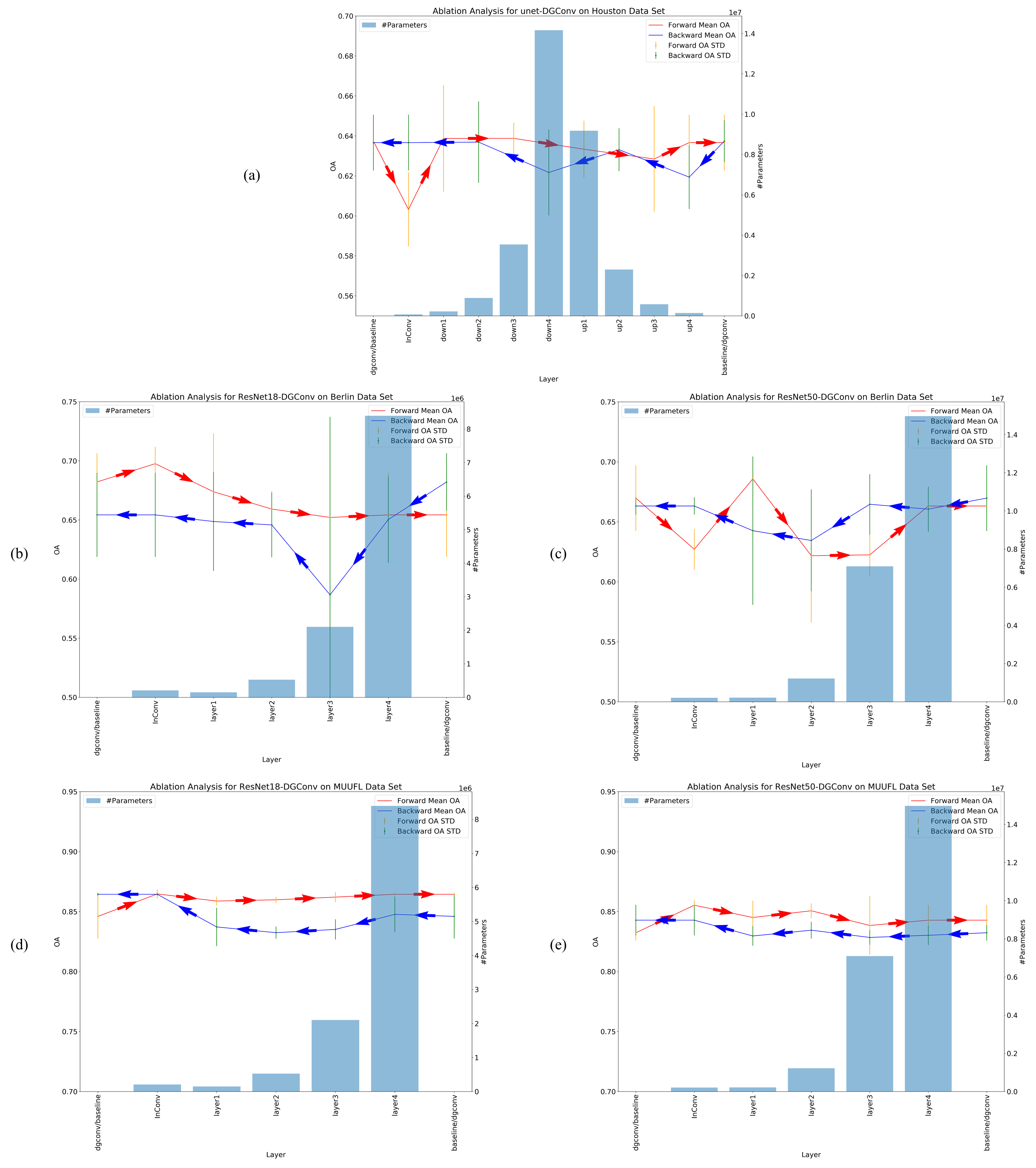
Figure 9: Classification performance of various models obtained via ablation analysis. The arrows indicate the order of removal of SepDGConv modules, while blue bars represent number of parameters in the corresponding block. (a) Performance of SepG-UNets on Houston2018 data set, (b) performance of SepG-ResNet18s on Berlin data set, (c) performance of SepG-ResNet50s on Berlin data set, (d) performance of SepG-ResNet18s on MUUFL data set, and (e) performance of SepG-ResNet50s on MUUFL data set,

To investigate the performance improvement of SepDGConv, we remove SepDGConv block-by-block from above models, and analyze the influence of SepDGConv’s usage on the overall performance. In particular, since separate convolution groups learned in a SepG-Net represents sensor-specific branches, we hope to shed light on whether such sensor-specificity is important for multi-source RS data fusion.

We design the ablation experiments based on the optimal brain damage (OBD) theory in DL [47], according to which if an important module in a deep neural network is removed, then significant performance drop should be observed. Concretely, for each SepDGConv model we run one forward pass and one backward pass. In the forward pass, we in order change SepDGConv in the following blocks back to regular convolution: [InConv, Layer1, Layer2, Layer3, Layer4] for SepG-ResNet, and [InConv, Down1, Down2, Down3, Down4, Up1, Up2, Up3, Up4] for SepG-UNet. In the backward pass, the order is reversed. The obtained models are retrained. For each model, the baseline, SepDGConv derivative, forward pass and backward pass are trained under one same configuration of hyperparameters.

The results of ablation experiments are shown in Fig. 9. We run each model 5 times with random seeds 42-46, same as our main experiment above. The value of each data point in Fig. 9 is taken as average OA of the 5 replicas, while each error bar represents standard deviation of 5 OA values. The red line represents OA changes in a forward pass, while the blue line represents OA changes in a backward pass. A data point in a forward pass means that all SepDGConvs in blocks previous to and including this point are replaced with regular convolution. For example, in Fig. 9(b) a point at Layer1 represents results from ResNet18s that have regular convolution in InConv and Layer1, and SepDGConv in Layer2-4. Similarly, a data point in a backward pass means that all SepDGConvs in blocks behind and including this point are replaced with regular convolution, while blocks previous to this point remain using SepDGConv.

In forward passes, performance gain is consistently observed in early stage of each pass. For example, in Fig. 9(b), on Berlin data set SepG-ResNet18’s performance improves as SepDGConv is removed from InConv and an OA of $69.76\%$ is obtained, which surpasses both the original SepG-Net as well as the baseline. Same performance gain can be observed in Fig. 9(d) and 9(e), when SepDGConv in InConv is replaced by regular convolution. According to OBD theory, this phenomenon implies that, rather than being beneficial to model performance, imposing multi-stream architecture in shallow layers actually harms model performance. For SepG-ResNet50 on Berlin data set, as shown in Fig. 9(c), while there is an initial performance loss, the OA goes up to $68.58\%$ as soon as SepDGConv layers in both InConv and Layer1 are removed, which means that at this point the shallow layers in the model are densely connected rather than having a multi-stream, sensor-specific architecture. A very similar loss-gain curve is observed on SepG-UNet, as shown in Fig. 9(a). Hence experimental results of SepG-ResNet50 on Berlin data set and SepG-UNet on Houston2018 data set both support our finding that for the first few blocks dense convolution is better than multi-stream convolution.

In backward passes, performance loss is observed as SepDGConv in middle and deep layers are removed. For UNet, the performance loss occurs as the backward pass goes through middle blocks, from Up1 to Down4, as shown in Fig. 9(a). For ResNets, we observe OA drop when SepDGConv in the last two blocks, Layer4 and Layer3, is replaced, as shown in Fig 9(b)-(d).

Furthermore, based on the distribution of number of parameters in the studied models, shown as the blue bars in Fig. 9, we summarize the performance loss in middle and last layers into a more general phenomenon, i.e., performance loss in wide layers. Wide layers refer to layers with more feature map channels, and thus with more parameters. It can be seen from Fig. 9 that for UNet the wide layers are Down3-Up2, exactly where we observe performance loss, and for ResNets the wide layers are Layer3-Layer4, where performance loss in the backward pass is also observed. Such performance loss implies that SepDGConv is beneficial to model performance if applied to wide layers.

Finally we shall revisit the performance gain phenomenon observed in the early stage of forward passes. This phenomenon occurs in the first few layers of studied models, where there are fewer parameters, as shown in Fig. 9. These layers are also called narrow layers, in accordance with ”wide layers”. Thus we can say that there is performance gain if we replace SepDGConv with regular convolution in narrow layers. Such performance gain implies that SepDGConv is harmful to model performance if applied to narrow, usually shallow layers. Besides, in Fig. 9(b)-(e), performance gain is observed in backward passes going from Layer2 to InConv. This is also a clue that dense convolution in narrow layers is more favorable to model performance.

To summarize, in the ablation analysis we observe that there is model performance gain if we replace SepDGConv with regular convolution in narrow, usually the first few layers in a model, and there is model performance loss if we replace SepDGConv with regular convolution in wide, usually the last few layers in a model. These findings imply that multi-stream architecture is harmful to model performance if used in narrow layers, but becomes beneficial if applied to wide layers.

IV-D Comparing different convolution strategies

TABLE VII: Different Convolution Strategies on UNet, Houston2018 Data Set

	UNet	GConv	FGConv	SepDGConv	Ablation	False Group
OA (%)	63.66±1.89	65.14±2.52	65.49±0.62	63.74±1.05	63.88±0.79	65.33±1.51

Results of our ablation analysis suggest that it is better to use regular convolution than SepDGConv in the first few layers of a CNN. This indicates that may not be playing an important role in data fusion models, since by using densely connected convolution the model no longer has sensor-specific features. However, SepDGConv also regularizes the model and the effect of sensor-specificity is not yet isolated from regularization. In this subsection, we further compare models using SepDGConv with another two convolution strategies that impose sensor-specific multi-branch architectures: group convolution (GConv) and fixed groupable convolution (FGConv).

As mentioned above (Sec. II(A)), by using GConv for the first $l$ layers and setting the number of groups to a fixed number $G_{0}$, a CNN with $G_{0}$ sensor-specific branches, each of depth $l$, can be built. In our experiments below we will use this strategy to construct models that have strictly sensor-specific branches, so we can better observe the effect of sensor-specificity. Specifically, for ResNets we will use GConv for [InConv, Layer 1-4], and for UNets we will use GConv for [InConv, Down1-4, Up1-4].

The role of FGConv is to further isolate sensor-specificity from regularization. Using SepDGConv does not guarantee sensor-specificity of deep layers, since the number of groups it learns varies from layer to layer. The idea of FGConv is to combine SepDGConv and GConv to make sure that any layer using FGConv has at least $G_{0}$ groups. Specifically, GConv can be equivalently expressed by an relationship matrix $U_{0}$ (Fig. 2(c)), and in FGConv we construct a new relationship matrix $U_{F}$ for a layer, using that layer’s learned SepDGConv relationship matrix $U$ and a specified GConv matrix $U_{0}$:

$$U_{F}=U_{0}\odot U$$ (16)

where $\odot$ denotes element-wise product. $U_{0}$ is constructed using the pre-specified group number $G_{0}$ and is fixed, while $U$ is still learned from data. In the experiments, FGConv is used in [InConv, Layer 1-4] for ResNets, and [InConv, Down1-4, Up1-4] for UNets.

For GConv, we make sure at the input layer that the group division leads to sensor-specificity, by manually designing the relationship matrix $U_{0}$. For Houston2018 data set, $U_{0}$ divides the 58 channel input data into 4 groups, mapping [3 MS, 48 HS, 3 LiDAR, 4 DEM/DSM] to [16, 16, 16, 16] feature maps. For Berlin data set, $U_{0}$ maps [244 HS, 4 SAR] to [32, 32] feature maps. For MUUFL data set, $U_{0}$ maps [64 HS, 2 LiDAR] to [32, 32] feature maps. The same $U_{0}$ is applied to FGConv.

Experimental results are shown in Table VII-XI. Performance of baseline models and SepG-models are cited from above, while the ”Ablation” column refers to the model’s best performance obtained in the ablation study. We report average and std of OA of 5 runs, using random seeds 42-46, same as above.

TABLE VIII: Different Convolution Strategies on ResNet18, Berlin Data Set

	ResNet18	GConv	FGConv	SepDGConv	Ablation
OA (%)	65.43±3.56	65.04±2.90	68.09±3.94	68.21±2.43	69.76±1.43

TABLE IX: Different Convolution Strategies on ResNet50, Berlin Data Set

	ResNet50	GConv	FGConv	SepDGConv	Ablation
OA (%)	66.98±2.73	65.90±1.24	64.85±3.07	66.32±0.72	68.58±1.57

TABLE X: Different Convolution Strategies on ResNet18, MUUFL Data Set

	ResNet18	GConv	FGConv	SepDGConv	Ablation
OA (%)	86.44±0.11	86.17±0.32	86.40±0.53	84.60±1.85	86.47±0.39

TABLE XI: Different Convolution Strategies on ResNet50, MUUFL Data Set

	ResNet50	GConv	FGConv	SepDGConv	Ablation
OA (%)	84.28±1.28	83.60±1.03	85.30±0.20	83.23±0.65	85.53±0.45

First consider the ResNets, Table VIII-XI. (1) It is consistently observed that baseline models marginally outperform the corresponding GConv models. This indicates that sensor-specific multi-branching does not necessarily help improve model performance. (2) In 3 out of total 4 experiments, i.e., except ResNet50 on Berlin data set, FGConv outperforms GConv. This supports our basic assumption that automatically learning group convolution hyperparameters benefits model performance. (3) In all of 4 experiments, neither does GConv nor does FGConv outperform the best architecture we previously find in the ablation study, where the models’ first few SepDGConv layers are relpaced with regular convolution. These models found in the ablation study do not have sensor-specific branches, so this result is consistent with (1).

Then consider the UNets on Houston2018 data set, Table VII. While in consistent with (2) above that FGConv outperforms GConv, for UNets we observe GConv outperforming baseline, SepDGConv and Ablation. To find an explanation for this we add a False-GConv experiment, where at the input layer we use a group division of [14, 16, 14, 14] instead of [2, 48, 3, 4], so that the 4 branches are no longer sensor-specific. False-GConv outperforms GConv while achieves slightly lower accuracy than FGConv. This implies that GConv and FGConv gains performance probably from the setting $G=4$, and again this experiment supports our finding above that sensor-specificity is not necessarily helpful.

IV-E Discussion

IV-E1 Multi-stream as regularization

Theoretically, both SepDGConv and human designed multi-stream deep neural networks can be regarded as regularization technique since it imposes certain constraints on the network architecture in order to reduce overfitting and to improve model performance [48] [49]. Based on our experiments and ablation analysis above, we attribute model performance in multi-source RS data fusion by using SepDGConv to regularization, for we have observed the following two very important features of regularization:

(1) Variance reduction. It is known that regularized models can generalize better, which means they should have less test variance. In our experiments, as discussed in Sec. III(B), except ResNet18 on MUUFL data set, all SepDGConv models have less test OA variance than their corresponding baseline models.

(2) Over-regularization. If a simple model is regularized too much, the model capacity can be reduced too much to fit the data, and as a result the overall model performance is harmed. In our ablation analysis, as shown in Fig. 9, we find out that imposing multi-stream SepDGConv on shallow layers leads to model performance loss. The most possible reason is that, these shallow, narrow layer themselves do not have many parameters, and by using SepDGConv they are over-regularized, leading to underfitting. On the other hand, the middle layers in UNet and last few layers in ResNets are much wider and have much more parameters than the first few layers, hence using SepDGConv on these wide layers very likely just achieves the expected regularization effect, improving the models’ performance.

Since we experiment with 3 different models on 3 very diverse data sets, our two findings above are highly generalizable, which provides strong clues that multi-stream architectures actually play the role of model regularizer.

Yet, regularization itself is a complex technique and its effect is always coupled with various aspects of model optimization and generalization, hence there are probably many other factors to explore that contribute to the phenomena we have observed. For example, a very recent paper [50] find out that one same model trained separately on different source of data acquired in the same area (RGB and SAR in their case) can lead to very similar model parameter distributions. This finding suggests that there could be feature redundancy in shallow layers of multi-stream architectures. Nevertheless, we hope our work shed some light on the mechanisms behind neural network architecture designing for multi-source RS data, and inspire novel research.

IV-E2 Possible improvements on group convolution

Our results suggest that models with regular convolution such as ResNet18 can obtain classification results at least comparable with SOTA methods, and that in shallow layers dense, regular convolution should be used, which together advocate single-stream deep CNN models for joint classification of multi-source RS data. To automatically learn grouped convolution in wide layers to utilize the regularization effect, it is more desirable if SepDGConv can learn dense convolution for narrow layers, and thus there is still room for improvement in SepDGConv. Besides, the restrictions SepDGConv puts on the relationship matrix $U$ are strong and in practice we may need to construct $U$s with more flexible structure. We hope novel research in constructing and learning the relationship matrix $U$ can lead to better single-stream CNN architectures for multi-source RS data.

IV-E3 Towards better performance

Our work makes it possible to build deep, single stream networks for multi-source RS data. On the one hand, modern techniques that boost model performance are more easily applied in a unified network. On the other hand, designing sufficiently large models is beneficial to, and probably necessary for, solving large-scale, real world RS problems.

In our paper, we only experiment and compare with basic models, leaving many techniques such as ensembling, and more complex modules such as attention mechanism to further improve model performance unexplored. For example, [28] utilizes Octave convolution and fractional Gabor convolution to propose a network that achieves SOTA OA of $89.90\%$ on MUUFL data set. We believe that such advanced modules, and more in the future, can be more easily implemented in a single-branch network.

Furthermore, as we can build models of comparable depth to those in modern CV research with our proposed technique, we can better utilize the benefits of overparametrized models, as well as potentially available large RS data in the future.

V CONCLUSION

In this paper we have investigated the potential of single-stream models in joint classification of multi-source remote sensing data. To enable multi-stream network structure to be automatically learned within a single-stream architecture, we propose the SepDGConv module based on group convolution and dynamic grouping convolution technique. With reference to modern deep convolutional neural network architectures, we then propose several deep learning models with SepDGConv: SepG-ResNet18, SepG-ResNet50, and SepG-UNet. The propsoed models are verified on three benchmark data sets with diverse data modality, yielding promising classification results, which indicate the effectiveness and generalizability of proposed single-stream networks for multi-source remote sensing data joint classification. Furthermore, we analyze the usage of SepDGConv in different parts of the models and find out that: (1) using SepDGConv generally reduces model variance, (2) using SepDGConv in narrow layers, usually the first few layers, harms model performance, and (3) using SepDGConv in wide layers, usually the last few layers, improves model performance. These findings imply that sensor-specific multi-stream architecture is essentially playing the role of model regularizer, and is not strictly necessary for multi-source remote sensing data fusion. We hope our work can inspire novel flexible and generalizable models for multi-source remote sensing data analysis.

References

- [1] J. Li, Y. Pei, S. Zhao, R. Xiao, X. Sang, and C. Zhang, “A review of remote sensing for environmental monitoring in china,” Remote Sensing, vol. 12, no. 7, p. 1130, 2020.
- [2] R. P. Sishodia, R. L. Ray, and S. K. Singh, “Applications of remote sensing in precision agriculture: A review,” Remote Sensing, vol. 12, no. 19, p. 3136, 2020.
- [3] Y. Xu, B. Du, L. Zhang, D. Cerra, M. Pato, E. Carmona, S. Prasad, N. Yokoya, R. Hänsch, and B. Le Saux, “Advanced multi-sensor optical remote sensing for urban land use and land cover classification: Outcome of the 2018 ieee grss data fusion contest,” IEEE Journal of Selected Topics in Applied Earth Observations and Remote Sensing, vol. 12, no. 6, pp. 1709–1724, 2019.
- [4] M. Pedergnana, P. R. Marpu, M. Dalla Mura, J. A. Benediktsson, and L. Bruzzone, “Classification of remote sensing optical and lidar data using extended attribute profiles,” IEEE Journal of Selected Topics in Signal Processing, vol. 6, no. 7, pp. 856–865, 2012.
- [5] M. Khodadadzadeh, J. Li, S. Prasad, and A. Plaza, “Fusion of hyperspectral and lidar remote sensing data using multiple feature learning,” IEEE Journal of Selected Topics in Applied Earth Observations and Remote Sensing, vol. 8, no. 6, pp. 2971–2983, 2015.
- [6] B. Rasti, P. Ghamisi, and R. Gloaguen, “Hyperspectral and lidar fusion using extinction profiles and total variation component analysis,” IEEE Transactions on Geoscience and Remote Sensing, vol. 55, no. 7, pp. 3997–4007, 2017.
- [7] Y. Gu, Q. Wang, X. Jia, and J. A. Benediktsson, “A novel mkl model of integrating lidar data and msi for urban area classification,” IEEE transactions on geoscience and remote sensing, vol. 53, no. 10, pp. 5312–5326, 2015.
- [8] J. Hu, D. Hong, and X. X. Zhu, “Mima: Mapper-induced manifold alignment for semi-supervised fusion of optical image and polarimetric sar data,” IEEE Transactions on Geoscience and Remote Sensing, vol. 57, no. 11, pp. 9025–9040, 2019.
- [9] G. Singh, F. Mémoli, G. E. Carlsson et al., “Topological methods for the analysis of high dimensional data sets and 3d object recognition.” PBG@ Eurographics, vol. 2, 2007.
- [10] Y. LeCun, Y. Bengio, and G. Hinton, “Deep learning,” nature, vol. 521, no. 7553, pp. 436–444, 2015.
- [11] Y. LeCun, K. Kavukcuoglu, and C. Farabet, “Convolutional networks and applications in vision,” in Proceedings of 2010 IEEE international symposium on circuits and systems. IEEE, 2010, pp. 253–256.
- [12] D. Marmanis, M. Datcu, T. Esch, and U. Stilla, “Deep learning earth observation classification using imagenet pretrained networks,” IEEE Geoscience and Remote Sensing Letters, vol. 13, no. 1, pp. 105–109, 2015.
- [13] E. Maggiori, Y. Tarabalka, G. Charpiat, and P. Alliez, “Convolutional neural networks for large-scale remote-sensing image classification,” IEEE Transactions on geoscience and remote sensing, vol. 55, no. 2, pp. 645–657, 2016.
- [14] X. Yuan, J. Shi, and L. Gu, “A review of deep learning methods for semantic segmentation of remote sensing imagery,” Expert Systems with Applications, p. 114417, 2020.
- [15] W. Hu, Y. Huang, L. Wei, F. Zhang, and H. Li, “Deep convolutional neural networks for hyperspectral image classification,” Journal of Sensors, vol. 2015, 2015.
- [16] W. Li, G. Wu, F. Zhang, and Q. Du, “Hyperspectral image classification using deep pixel-pair features,” IEEE Transactions on Geoscience and Remote Sensing, vol. 55, no. 2, pp. 844–853, 2016.
- [17] H. Lee and H. Kwon, “Going deeper with contextual cnn for hyperspectral image classification,” IEEE Transactions on Image Processing, vol. 26, no. 10, pp. 4843–4855, 2017.
- [18] X. He, A. Wang, P. Ghamisi, G. Li, and Y. Chen, “Lidar data classification using spatial transformation and cnn,” IEEE Geoscience and Remote Sensing Letters, vol. 16, no. 1, pp. 125–129, 2018.
- [19] S. Pan, H. Guan, Y. Chen, Y. Yu, W. N. Gonçalves, J. M. Junior, and J. Li, “Land-cover classification of multispectral lidar data using cnn with optimized hyper-parameters,” ISPRS Journal of Photogrammetry and Remote Sensing, vol. 166, pp. 241–254, 2020.
- [20] J. Zhao, W. Guo, S. Cui, Z. Zhang, and W. Yu, “Convolutional neural network for sar image classification at patch level,” in 2016 IEEE International Geoscience and Remote Sensing Symposium (IGARSS). IEEE, 2016, pp. 945–948.
- [21] M. Ma, J. Chen, W. Liu, and W. Yang, “Ship classification and detection based on cnn using gf-3 sar images,” Remote Sensing, vol. 10, no. 12, p. 2043, 2018.
- [22] Y. Chen, C. Li, P. Ghamisi, X. Jia, and Y. Gu, “Deep fusion of remote sensing data for accurate classification,” IEEE Geoscience and Remote Sensing Letters, vol. 14, no. 8, pp. 1253–1257, 2017.
- [23] X. Xu, W. Li, Q. Ran, Q. Du, L. Gao, and B. Zhang, “Multisource remote sensing data classification based on convolutional neural network,” IEEE Transactions on Geoscience and Remote Sensing, vol. 56, no. 2, pp. 937–949, 2017.
- [24] Y. Xu, B. Du, and L. Zhang, “Multi-source remote sensing data classification via fully convolutional networks and post-classification processing,” in IGARSS 2018-2018 IEEE International Geoscience and Remote Sensing Symposium. IEEE, 2018, pp. 3852–3855.
- [25] D. Hong, L. Gao, N. Yokoya, J. Yao, J. Chanussot, Q. Du, and B. Zhang, “More diverse means better: Multimodal deep learning meets remote-sensing imagery classification,” IEEE Transactions on Geoscience and Remote Sensing, vol. 59, no. 5, pp. 4340–4354, 2020.
- [26] D. Hong, N. Yokoya, G.-S. Xia, J. Chanussot, and X. X. Zhu, “X-modalnet: A semi-supervised deep cross-modal network for classification of remote sensing data,” ISPRS Journal of Photogrammetry and Remote Sensing, vol. 167, pp. 12–23, 2020.
- [27] M. Zhang, W. Li, R. Tao, H. Li, and Q. Du, “Information fusion for classification of hyperspectral and lidar data using ip-cnn,” IEEE Transactions on Geoscience and Remote Sensing, 2021.
- [28] X. Zhao, R. Tao, W. Li, W. Philips, and W. Liao, “Fractional gabor convolutional network for multisource remote sensing data classification,” IEEE Transactions on Geoscience and Remote Sensing, 2021.
- [29] R. Hang, Z. Li, P. Ghamisi, D. Hong, G. Xia, and Q. Liu, “Classification of hyperspectral and lidar data using coupled cnns,” IEEE Transactions on Geoscience and Remote Sensing, vol. 58, no. 7, pp. 4939–4950, 2020.
- [30] C. Hazirbas, L. Ma, C. Domokos, and D. Cremers, “Fusenet: Incorporating depth into semantic segmentation via fusion-based cnn architecture,” in Asian conference on computer vision. Springer, 2016, pp. 213–228.
- [31] N. Audebert, B. Le Saux, and S. Lefèvre, “Beyond rgb: Very high resolution urban remote sensing with multimodal deep networks,” ISPRS Journal of Photogrammetry and Remote Sensing, vol. 140, pp. 20–32, 2018.
- [32] K. Chen, K. Fu, X. Gao, M. Yan, W. Zhang, Y. Zhang, and X. Sun, “Effective fusion of multi-modal data with group convolutions for semantic segmentation of aerial imagery,” in IGARSS 2019-2019 IEEE International Geoscience and Remote Sensing Symposium. IEEE, 2019, pp. 3911–3914.
- [33] A. Khan, A. Sohail, U. Zahoora, and A. S. Qureshi, “A survey of the recent architectures of deep convolutional neural networks,” Artificial Intelligence Review, vol. 53, no. 8, pp. 5455–5516, 2020.
- [34] Z. Zhang, J. Li, W. Shao, Z. Peng, R. Zhang, X. Wang, and P. Luo, “Differentiable learning-to-group channels via groupable convolutional neural networks,” in Proceedings of the IEEE/CVF International Conference on Computer Vision, 2019, pp. 3542–3551.
- [35] A. Krizhevsky, I. Sutskever, and G. E. Hinton, “Imagenet classification with deep convolutional neural networks,” Advances in neural information processing systems, vol. 25, pp. 1097–1105, 2012.
- [36] S. Xie, R. Girshick, P. Dollár, Z. Tu, and K. He, “Aggregated residual transformations for deep neural networks,” in Proceedings of the IEEE conference on computer vision and pattern recognition, 2017, pp. 1492–1500.
- [37] P. Yin, J. Lyu, S. Zhang, S. Osher, Y. Qi, and J. Xin, “Understanding straight-through estimator in training activation quantized neural nets,” in International Conference on Learning Representations, 2019.
- [38] K. He, X. Zhang, S. Ren, and J. Sun, “Deep residual learning for image recognition,” in Proceedings of the IEEE conference on computer vision and pattern recognition, 2016, pp. 770–778.
- [39] O. Ronneberger, P. Fischer, and T. Brox, “U-net: Convolutional networks for biomedical image segmentation,” in International Conference on Medical image computing and computer-assisted intervention. Springer, 2015, pp. 234–241.
- [40] A. Okujeni, S. van der Linden, and P. Hostert, “Berlin-urban-gradient dataset 2009-an enmap preparatory flight campaign,” 2016.
- [41] D. Hong, J. Hu, J. Yao, J. Chanussot, and X. X. Zhu, “Multimodal remote sensing benchmark datasets for land cover classification with a shared and specific feature learning model,” ISPRS Journal of Photogrammetry and Remote Sensing, vol. 178, pp. 68–80, 2021.
- [42] X. Du and A. Zare, “Technical report: scene label ground truth map for muufl gulfport data set,” University of Florida, Gainesville, FL., Tech. Rep. Tech. Rep. 20170417, April 2017. [Online]. Available: http://ufdc.ufl.edu/IR00009711/00001
- [43] D. Cerra, M. Pato, E. Carmona, S. M. Azimi, J. Tian, R. Bahmanyar, F. Kurz, E. Vig, K. Bittner, C. Henry et al., “Combining deep and shallow neural networks with ad hoc detectors for the classification of complex multi-modal urban scenes,” in IGARSS 2018-2018 IEEE International Geoscience and Remote Sensing Symposium. IEEE, 2018, pp. 3856–3859.
- [44] D. P. Kingma and J. Ba, “Adam: A method for stochastic optimization,” arXiv preprint arXiv:1412.6980, 2014.
- [45] K. He, X. Zhang, S. Ren, and J. Sun, “Delving deep into rectifiers: Surpassing human-level performance on imagenet classification,” in Proceedings of the IEEE international conference on computer vision, 2015, pp. 1026–1034.
- [46] P. Goyal, P. Dollár, R. Girshick, P. Noordhuis, L. Wesolowski, A. Kyrola, A. Tulloch, Y. Jia, and K. He, “Accurate, large minibatch sgd: Training imagenet in 1 hour,” arXiv preprint arXiv:1706.02677, 2017.
- [47] Y. LeCun, J. S. Denker, and S. A. Solla, “Optimal brain damage,” in Advances in neural information processing systems, 1990, pp. 598–605.
- [48] I. Goodfellow, Y. Bengio, and A. Courville, Deep learning. MIT press, 2016.
- [49] J. Kukačka, V. Golkov, and D. Cremers, “Regularization for deep learning: A taxonomy,” arXiv preprint arXiv:1710.10686, 2017.
- [50] Z. Zheng, A. Ma, L. Zhang, and Y. Zhong, “Deep multisensor learning for missing-modality all-weather mapping,” ISPRS Journal of Photogrammetry and Remote Sensing, vol. 174, pp. 254–264, 2021.