Time crystals: From Schrödinger to Sisyphus
 

Abstract

A Hamiltonian time crystal can emerge when a Noether symmetry is subject to a condition that prevents the energy minimum from being a critical point of the Hamiltonian. A somewhat trivial example is the Schrödinger equation of a harmonic oscillator. The Noether charge for its particle number coincides with the square norm of the wave function, and the energy eigenvalue is a Lagrange multiplier for the condition that the wave function is properly normalized. A more elaborate example is the Gross-Pitaevskii equation that models vortices in a cold atom Bose-Einstein condensate. In an oblate, essentially two dimensional harmonic trap the energy minimum is a topologically protected timecrystalline vortex that rotates around the trap center. Additional examples are constructed using coarse grained Hamiltonian models of closed molecular chains. When knotted, the topology of a chain can support a time crystal. As a physical example, high precision all-atom molecular dynamics is used to analyze an isolated cyclopropane molecule. The simulation reveals that the molecular D_3h symmetry becomes spontaneously broken. When the molecule is observed with sufficiently long stroboscopic time steps it appears to rotate like a simple Hamiltonian time crystal. When the length of the stroboscopic time step is decreased the rotational motion becomes increasingly ratcheting and eventually it resembles the back-and-forth oscillations of Sisyphus dynamics. The stroboscopic rotation is entirely due to atomic level oscillatory shape changes, so that cyclopropane is an example of a molecule that can rotate without angular momentum. Finally, the article is concluded with a personal recollection how Frank’s and Betsy’s Stockholm journey started.
Based on talk at Frankfest, Högberga 2021

I 1. Introduction

Wilczek  wilczek-2012 together with Shapere  shapere-2012b envisioned a time crystal to be a state that extends the notion of spontaneous breakdown of space translation symmetry to include time translation symmetry. They argued that if time translation symmetry becomes spontaneously broken, the lowest energy state of a physical system can no longer be time independent but has to change with time. If the symmetry breaking leaves behind a discrete group the ensuing time evolution will be periodic, and in analogy with space crystals we have a time crystal.

The proposal drew immediate criticism: In a canonical Hamiltonian setting the generator of time translations is the Hamiltonian itself. Thus energy is a conserved charge. But if time translation symmetry becomes spontaneously broken, the ground state energy can no longer be a conserved quantity. Accordingly, a time crystal must be impossible in any kind of isolated and energy conserving physical system, governed by autonomous Hamiltonian equation of motion  bruno-2013 ; watabane-2015 ; yamamoto-2015 .

As a consequence the search of spontaneously broken time translation symmetry focused on driven, non-equilibrium quantum systems  Sacha-2015 ; Sacha-2016 ; khemani-2016 ; else-2016a ; else-2016 ; else-2016b ; Yao-2017 . The starting point is a many-body system with intrinsic dynamics governed by a time independent Hamiltonian $H$. The system is then subjected to an external explicitly time periodic driving force, with period $T$, that derives from an extrinsic time dependent potential $U(t+T)=U(t)$. The total Hamiltonian is the sum of the two $H_{tot}(t)=H+U(t)$ so that the total Hamiltonian is also explicitly time dependent, with the same period $T$ of the drive. Floquet theory asserts that there can be solutions to the corresponding time dependent Schrödinger equation, with a time period that is different from $T$ where the difference is due to a Floquet index. As a consequence it is plausible that in such a periodically driven many-body system, a spontaneous self-organization of time periodicity takes place so that the system starts evolving with its own characteristic period, which is different from that of the external driving force. It was first shown numerically that this kind of self-organisation can take place in certain many-body localized spin systems  Sacha-2015 ; Sacha-2016 ; khemani-2016 ; else-2016a ; else-2016 ; else-2016b ; Yao-2017 . Experiments were then performed in appropriate material realizations  zhang-2017 ; lukin-2017 ; Rovny-2018 and they confirmed the presence of sustained collective oscillations with a time period that is indeed different from the period of the external driving force. It is now widely accepted that this kind of driven non-equilibrium Floquet time crystals do exist, but the setting is quite distant from Wilczek’s original idea.

Here I describe how, in spite of the No-Go arguments, genuine (semi)classical and quantum Hamiltonian time crystals do exist Dai-2019 ; anton ; Dai-2020 . They could even be widespread. I start with an explicit proof-of-concept construction that shows how to go around the No-Go arguments: I show that whenever a Hamiltonian system supports conserved Noether charges that are subject to appropriate conditions, the lowest energy ground state can be both time dependent and have an energy value that is conserved. This can occur whenever the lowest energy ground state, as a consequence of the conditions, is not a critical point of the Hamiltonian. I explain how such a time dependent ground state can be explicitly constructed by the methods of constrained optimization Fletcher-1987 ; Nocedal-1999 , using the Lagrange multiplier theorem Marsden . Whenever the solution for any Lagrange multiplier is non-vanishing, the lowest energy ground state is time dependent: A time crystal is simply a time dependent symmetry transformation that converts the time evolution of a Hamiltonian system into an equivariant time evolution. In particular, since time translation symmetry is not spontaneously broken but equivariantized, unlike in the case of conventional spontaneous symmetry breaking now there is no massless Goldstone boson that can be associated with a time crystal. But the two concepts can become related in a limit where the period of a time crystal goes to infinity and its energy approaches a (degenerate) critical point of the Hamiltonian.

I present a number of examples, starting with the time dependent Schrödinger equation of a harmonic oscillator. I continue with the Gross-Pitaevskii equation that models vortices in a cold atom Bose-Einstein condensate, and with a generalized Landau-Lifschitz equation that can describe closed molecular chains in a coarse grained approximation. I then analyze cyclopropane as an actual molecular example of timecrystalline Hamiltonian dynamics. For this I employ high precision all-atom molecular dynamics to investigate the ground state properties of a single isolated cyclopropane molecule. I conclude that the maximally symmetric configuration, with the D_3h molecular symmetry, can become spontaneously broken. I follow the time evolution of the minimum energy configuration stroboscopically, at very low but constant internal temperature values. I find that with a proper internal temperature and for sufficiently long stroboscopic time steps the molecule becomes a Hamiltonian time crystal with time evolution that is described by the generalization of the Landau-Lifschitz equation. But when the length of the stroboscopic time step is decreased, there is a cross-over transition to an increasingly ratcheting time evolution. In the limit where the stroboscopic time step is very small the motion of the cyclopropane molecule resembles Sisyphus dynamics  sisyphus . I propose that this kind of cross-over transition between the Sisyphus dynamics that describes the limit of very short stroboscopic time steps, and the uniform timecrystalline dynamics that describes the limit of very long stroboscopic time steps, is a universal phenomenon. It exemplifies that the coarse graining of an apparently random microscopic many-body system can lead to a separation of scales and self-organization towards an effective theory Hamiltonian time crystal.

Finally, the rotational motion that I observe in a cyclopropane in the limit of long stroboscopic time steps, can occur even with no angular momentum. Thus, cyclopropane is a molecular level example of a general phenomenon of rotation by shape deformation, and without any angular momentum: The short time scale vibrational motions of the individual atoms that are driven e.g. by thermal or maybe even by quantum mechanical zero point fluctuations can become converted into a large scale rotational motion of the entire molecule, even when there is no angular momentum. This kind of phenomenon was first predicted by Guichardet Guichardet-1984 , and independently by Shapere and Wilczek Shapere-1989b , and an early review can be found in  Littlejohn .

II 2. Hamiltonian time crystals

A Hamiltonian time crystal describes the minimum of a Hamiltonian that is not a critical point of the Hamiltonian. To show how this can occur, I start with the Hamiltonian action

$$S=\int dt\ p_{i}\dot{q}_{i}-H(p,q)$$ (1)

where ($p_{i},q_{i}$) ($i,j=1,...,N$) are the local Darboux coordinates with non-vanishing Poisson bracket

$$\{q_{i},p_{j}\}=\delta_{ij}$$ (2)

and Hamilton’s equation is

$$\begin{split}&\frac{dq_{i}}{dt}=\{q_{i},H\}=\ \ \frac{\partial H}{\partial p_{i}}\\ &\frac{dp_{i}}{dt}=\{p_{i},H\}=-\frac{\partial H}{\partial q_{i}}\end{split}$$ (3)

On a compact closed manifold the minimum of $H(p,q)$ is also its critical point, and in that case the Hamiltonian can not support any time crystal bruno-2013 ; watabane-2015 ; yamamoto-2015 . Thus for a time crystal we need additional structure, and for this I focus on a canonical Hamiltonian system that is subject to appropriate conditions

$$G_{a}(p,q)-g_{a}=0\ \ \ \ \ \ \ \ \ \ \ \ a=1,...,n\leq N$$ (4)

where the $g_{a}$ are some constants and the $G_{a}$’s define a Noether symmetry,

$$\begin{split}\{G_{a},G_{b}\}=&\ f_{abc}G_{c}\ \ \ \ \ \ {\rm for\ \ all}\ \ a,b,c\\ \{G_{a},H\}=&\ 0\end{split}$$ (5)

I then search for a solution to the following problem anton :

First, find a minimum of $H(p,q)$ that is subject to appropriate conditions (4) but is not a

critical point of $H(p,q)$. Then, solve (3) with this minimum as the initial condition.

The first step is a classic problem in constrained optimization Fletcher-1987 ; Nocedal-1999 and it can be solved using the Lagrange multiplier theorem Marsden . The theorem states that the minimum of $H$ can be found as a critical point of

$$H_{\lambda}(p,q;\lambda)\ =\ H(p,q)+\lambda_{a}(G_{a}(p,q)-g_{a})$$ (6)

where the $\lambda_{a}$ are independent, a priori time dependent auxiliary variables. The critical point of (6) is a solution of

$$\begin{split}&\frac{\partial H}{\partial p_{i}}+\lambda_{a}\frac{\partial G_{a}}{\partial p_{i}}\ =\ 0\\ &\frac{\partial H}{\partial q_{i}}+\lambda_{a}\frac{\partial G_{a}}{\partial q_{i}}\ =\ 0\\ &G_{a}(p,q)\ =\ g_{a}\end{split}$$ (7)

Since the number of equations (7) equals the number of unknowns ($p,q,\lambda$) a solution ($p^{\star},q^{\star},\lambda^{\star}$) including the Lagrange multiplier, can be found at least in principle. Under proper conditions, in particular if $H(p,q)$ is strictly convex and the $G^{a}(p,q)$ are affine functions, existence and uniqueness theorems can also be derived. But if there are more than one solution I choose the one with the smallest value of $H(p,q)$.

Suppose the solutions $\lambda^{\star}_{a}$ for the Lagrange multipliers do not all vanish. By combining (7) with (3) I conclude that I have a time crystal anton with the initial condition

$$p_{i}(t=0)=p_{i}^{\star}\ \ \ \ \&\ \ \ \ q_{i}(t=0)=q_{i}^{\star}\ \ \ \ \&\ \ \ \ \lambda_{a}(t=0)=\lambda_{a}^{\star}$$ (8)

and with the time evolution

$$\begin{split}&\frac{dq_{i}}{dt}\ =\ -\lambda_{a}^{\star}\frac{\partial G_{a}}{\partial p_{i}}\ =\ -\lambda_{a}^{\star}\{q_{i},G_{a}\}\\ &\frac{dp_{i}}{dt}\ =\ \ \ \lambda_{a}^{\star}\frac{\partial G_{a}}{\partial q_{i}}\ =\ -\lambda_{a}^{\star}\{p_{i},G_{a}\}\end{split}$$ (9)

and the Lagrange multipliers can be shown to be time independent $\lambda_{a}(t)\equiv\lambda_{a}^{\star}$. In particular, the timecrystalline evolution (9) determines a time dependent symmetry transformation of the minimum energy configuration (8), one that is generated by the linear combination

$$G^{\lambda}_{a}\ =\ \lambda_{a}^{\star}G_{a}$$

of the Noether charges.

Since the Hamiltonian $H$ has no explicit time dependence I immediately conclude that the energy of the time crystal is a conserved quantity

$$\frac{dH}{dt}\ =\ -\lambda_{a}^{\star}\{H,G_{a}\}\ =\ 0$$

This contrasts some of the early arguments, to exclude a time crystal on the grounds that the minimum energy should be time dependent.

In the sequel I consider exclusively such energy conserving Hamiltonian time crystals, with a time evolution that is a symmetry transformation.

III 3. Schrödinger as time crystal

For a simple example of the general formalism, I start with the following canonical action

$$S=\int dtd\mathbf{x}\ \{\ \bar{\psi}(i\partial_{t})\psi-\bar{\psi}(-{\nabla}^{2}+|\mathbf{x}|^{2})\psi\ \}$$ (10)

in $D$ space dimensions. This action yields the non-vanishing Poisson bracket

$$\{\bar{\psi}(\mathbf{x}_{1}),\psi(\mathbf{x}_{2})\}=-i\delta(\mathbf{x}_{1}-\mathbf{x}_{2})$$ (11)

The Hamiltonian energy is

$$H\ =\ \int d\mathbf{x}\,\bar{\psi}(-\nabla^{2}+|\mathbf{x}|^{2})\psi$$ (12)

and Hamilton’s equation coincides with the time dependent Schrödinger equation

$$i\partial_{t}\psi=-\nabla^{2}\psi+|\mathbf{x}|^{2}\psi$$ (13)

The Hamiltonian is strictly convex and its unique critical point is the absolute minimum

$$\psi(\mathbf{x})\ =\ 0$$

At this point I have an example of the situation governed by (3). In particular, there is no time crystal, as defined in the previous Section.

To obtain a time crystal I follow the general formalism of the previous section: I introduce the square norm

$$N=\int d\mathbf{x}\ \bar{\psi}\psi$$ (14)

This is the Noether charge for the symmetry of (10) under a phase rotation, it counts the number of particles, and I subject it to the following familiar condition (4),

$$G_{1}\ \equiv\ N-1=(\int d\mathbf{x}\ \bar{\psi}\psi)\ -1\ =\ 0$$ (15)

I then proceed with the Lagrange multiplier theorem and search for the critical point of the corresponding functional (6)

$$H_{E}=\int d\mathbf{x}\,\bar{\psi}(-\nabla^{2}+|\mathbf{x}|^{2})\psi\ -\ E(\int d\mathbf{x}\ \bar{\psi}\psi\ -1)$$

Where $E\equiv-\lambda$ is the Lagrange multiplier: The corresponding equations (7) coincide with the time independent Schrödinger equation for a harmonic oscillator

$$\begin{split}&-\nabla^{2}\psi+|\mathbf{x}|^{2}\psi=E\psi\\ &\int d\mathbf{x}\ \bar{\psi}\psi=1\end{split}$$

In general there are many solutions, all the harmonic oscillator eigenstates are solutions. But I pick up the solution ($\psi_{min}^{\star}(\mathbf{x}),E_{min}^{\star}$) that minimizes the energy (12). This is exactly the textbook lowest energy ground state wave function $\psi_{min}^{\star}(\mathbf{x})$ of the $D$ dimensional harmonic oscillator, and $E_{min}^{\star}$ is the corresponding lowest energy eigenvalue.

In line with (8), (9) I can write the time dependent Schrödinger equation (13) as follows,

$$i\partial_{t}\psi\ =\ E_{min}^{\star}\{N,\psi\}\ \equiv\ E_{min}^{\star}\{\int\bar{\psi}\psi,\psi\}\ \ \ \ \ \ {\rm with}\ \ \ \ \ \ \psi(\mathbf{x},t=0)\ =\ \psi_{min}^{\star}(\mathbf{x})$$ (16)

That is, the time evolution of the harmonic oscillator wave function is a symmetry transformation generated by the Noether charge $N$ i.e. a phase rotation, with the familiar solution

$$\psi(\mathbf{x},t)=e^{-iE_{min}^{\star}t}\,\psi_{min}^{\star}(\mathbf{x})$$ (17)

Normally, a time dependent phase factor is not an observable. But it can be made so, e.g. in a proper double slit experiment. Note that unlike in the case of standard spontaneous symmetry breaking, even though time translation invariance is converted into an equivariant time translation, there is no Goldstone boson in a quantum harmonic oscillator.

The previous example is verbatim a realization of the general formalism in Section 2. Albeit quite elementary in its familiarity and simplicity, it nevertheless makes the point. Conditions such as (4) on Noether charges are commonplace, they often have a pivotal role in specifying the physical scenario. When that happens, a time crystal can appear. Moreover, without additional structure the appearance of a time crystal does not entail the emergence of a massless Goldstone boson: A time crystal does not break the time translation symmetry. Instead, it equivariantizes a time translation into a combination of a time translation and a symmetry transformation.

IV 4. Nonlinear Schrödinger and time crystalline vortices

I now proceed with additional examples of the general formalism. For this I observe that besides phase rotations generated by the Noether charge $N$, the Schrödinger action (10) has also a Noether symmetry under space rotations. Accordingly I introduce the corresponding Noether charges

$$\mathbf{L}\ =\ \int d\mathbf{x}\,\bar{\psi}(-i\mathbf{x}\wedge\nabla)\psi\,$$

Their Poisson brackets coincide with the Lie algebra $SO(D)$ in $D$ dimensions, and have vanishing Poisson brackets with the conserved charge (14),

$$\{\mathbf{L},N\}=0$$

I follow the general formalism: I impose additional conditions to the harmonic oscillator using the maximal commuting subalgebra of space rotations; in three dimensions this amount to the familiar conditions $\mathbf{L}^{2}=l(l+1)$ and $L_{z}=m$ with $l\in\mathbb{Z}^{+}$ and $m\in\mathbb{Z}$ and $|m|\leq l$. I can take results from any quantum mechanics textbook and confirm that all the higher angular momentum eigenstates of the harmonic oscillator yield the appropriate minimum energy solutions of the time dependent Schrödinger equation.

For a more elaborate structure, I introduce a quartic self-interaction and consider the following nonlinear Schrödinger action,

$$S=\int dtd\mathbf{x}\ \{\ \bar{\psi}(i\partial_{t})\psi-\bar{\psi}(-\nabla^{2}+|\mathbf{x}|^{2})\psi-\frac{g}{2}(\bar{\psi}\psi)^{2}\ \}$$ (18)

This action also supports both $N$ and $\mathbf{L}$ as conserved Noether charges. It defines the Gross-Pitaevskii model that describes e.g. the Bose-Einstein condensation of cold alkali atoms at the level of a mean field theory sonin , with $g>0$ the quartic nonlinearity models short distance two-body repulsion. For clarity I specify to two space dimensions so that there is only one conserved charge $L\equiv L_{z}$. The set-up is that of a spheroidal, highly oblate three dimensional trap, with atoms confined to a disk by a very strong trap potential in the $z$-direction, and much weaker harmonic trap potential in the ($x,y$) direction. Thus, besides the condition (15) I also introduce the following condition

$$G_{2}\ \equiv\ L_{z}-l_{z}\ =\ \int dxdy\ \bar{\psi}(-i\mathbf{x}\times\nabla)\psi\ -\ l_{z}\ =\ 0$$ (19)

so that I have the scenario (4), (5) with two Noether charges.

I keep the normalization (15) but I leave the numerical value $l_{z}$ of the angular momentum as a free parameter. The choice (15) is entirely for convenience: I can always rescale the square norm to set $N$ to any non-vanishing value, and compensate for this by adjusting the length and time scales. But $l_{z}$ and the parameter $g$ in (18) remain as freely adjustable parameters Garaud-2021a . Note that even though the microscopic, individual atom angular momentum is certainly quantized, the macroscopic angular momentum $L_{z}$ does not need to be quantized: In applications to cold atoms the wave function $\psi(x,y)$ is a macroscopic condensate wave function that describes a very large number of atoms. Thus, it can support arbitrary values of the macroscopic angular momentum $L_{z}$.

Following Garaud-2021a I search for a solution of the nonlinear time dependent Schrödinger equation of (18) a.k.a. the Gross-Pitaevskii equation

$$i\partial_{t}\psi=-\nabla^{2}\psi+|\mathbf{x}|^{2}\psi+g|\psi|^{2}\psi$$ (20)

that minimizes the Hamiltonian i.e. energy

$$H=\int d\mathbf{x}\ \{\bar{\psi}(-\nabla^{2}+|\mathbf{x}|^{2})\psi+\frac{g}{2}(\bar{\psi}\psi)^{2}\}$$ (21)

subject to the two conditions (15) and (19). The Hamiltonian is strictly convex, its global minimum coincides with the only critical point $\psi(\mathbf{x})\equiv 0$. But when it is subject to the conditions (15) and (19) the minimum does not longer need to be a critical point. Instead, the Lagrange multiplier theorem states that the minimum is a critical point ($\psi^{\star},\lambda_{1}^{\star},\lambda_{2}^{\star}$) of

$$H_{\lambda}\ =\ H+\lambda_{1}G_{1}+\lambda_{2}G_{2}$$ (22)

That is, the minimum is a solution of

$$\begin{split}&\frac{\delta H_{\lambda}}{\delta\psi}\ =\ -\nabla^{2}\psi+|\mathbf{x}|^{2}\psi+g|\psi|^{2}\psi+\lambda_{1}\psi+\lambda_{2}(-i\mathbf{x}\times\nabla)\psi=0\\ &\frac{\delta H_{\lambda}}{\delta\lambda_{1}}\ =\ \int d\mathbf{x}\ \bar{\psi}\psi-1=0\\ &\frac{\delta H_{\lambda}}{\delta\lambda_{2}}\ =\ \int d\mathbf{x}\ \bar{\psi}(-i\mathbf{x}\times\nabla)\psi\ -l_{z}=0\end{split}$$ (23)

If there are several solutions, I choose ($\psi^{\star},\lambda_{1}^{\star},\lambda_{2}^{\star}$) for which $H(\psi)$ has the smallest value. The minimum energy $\psi^{\star}(\mathbf{x})$ then defines the initial condition

$$\psi(\mathbf{x},t=0)=\psi^{\star}(\mathbf{x})$$ (24)

for the putative timecrystalline solution of (20); recall that the corrresponding Lagrange multipliers are space-time independent, $\lambda_{1,2}(\mathbf{x},t)\equiv\lambda_{1,2}^{\star}$.

Remarkably, when I combine (23) and (20), the nonlinear time evolution equation of $\psi^{\star}(\mathbf{x})$ becomes converted to the following linear time evolution equation

$$i\partial_{t}\psi\ =\ -\lambda_{1}^{\star}\psi+i\lambda_{2}^{\star}\mathbf{x}\times\nabla\psi\ \equiv\ -\lambda_{1}^{\star}\{G_{1},\psi\}-\lambda_{2}^{\star}\{G_{2},\psi\}$$ (25)

This is the equation (9) in the present case. In particular, (25) states that the time evolution of $\psi^{\star}(\mathbf{x})$ is a symmetry transformation; the pertinent symmetry is a combination of phase rotation by $N$ and a spatial rotation by $L_{z}$.

Since the Hamiltonian $H$ has vanishing Poisson brackets with both $G_{1}$ and $G_{2}$, the energy is conserved during the timecrystalline evolution,

$$\frac{d}{dt}H\ =\ \lambda_{1}^{\star}\{H,G_{1}\}+\lambda_{2}^{\star}\{H,G_{2}\}=0$$

The solutions of (23), (20) describe vortices that rotate uniformly, with angular velocity $-\lambda_{2}^{\star}$ around of the trap center. For this I define

$$\mathbf{L}_{z}=-i\mathbf{x}\times\nabla\ \ \ \ \ \ \&\ \ \ \ \ \ \mathbf{A}=\nabla\tan^{-1}\left(\frac{x}{y}\right)$$

to write (25) as follows:

$$i\partial_{t}\psi=-\lambda_{2}^{\star}\left(\mathbf{L}_{z}+\frac{\lambda_{1}^{\star}}{\lambda_{2}^{\star}}\mathbf{x}\times\mathbf{A}\right)\psi\ \equiv\ \omega\mathbf{L}_{z}^{cov}\psi$$ (26)

Here $\mathbf{L}_{z}^{cov}$ is the covariant angular momentum that generates the rotations around the trap center in the presence of the ”analog gauge field” $\mathbf{A}$. Note that $\mathbf{A}$ supports a ”magnetic” flux with ”strength” $\lambda_{1}^{\star}/\lambda_{2}^{\star}$ along the $z$-axis, that can have non-integer values. Notably, $\mathbf{L}_{z}^{cov}$ has the same form as the angular momentum operator introduced by Wilczek Wilczek-1982a ; Wilczek-1982b , in the case of an anyon pair, in terms of the relative coordinate.

The Figure 1 summarizes the results from the numerical investigations in [ Ģaraud-2021a]. The number of vortices and their relative positions including the distances from the trap center, depend on the free parameter $l_{z}$. The two top lines of Figure 1 show how the phase and the cores of the vortex structure evolve for $0<l_{z}<2$. The bottom panels show the corresponding values of the Lagrange multipliers $\lambda_{1}^{\star}$ and $\lambda_{2}^{\star}$.

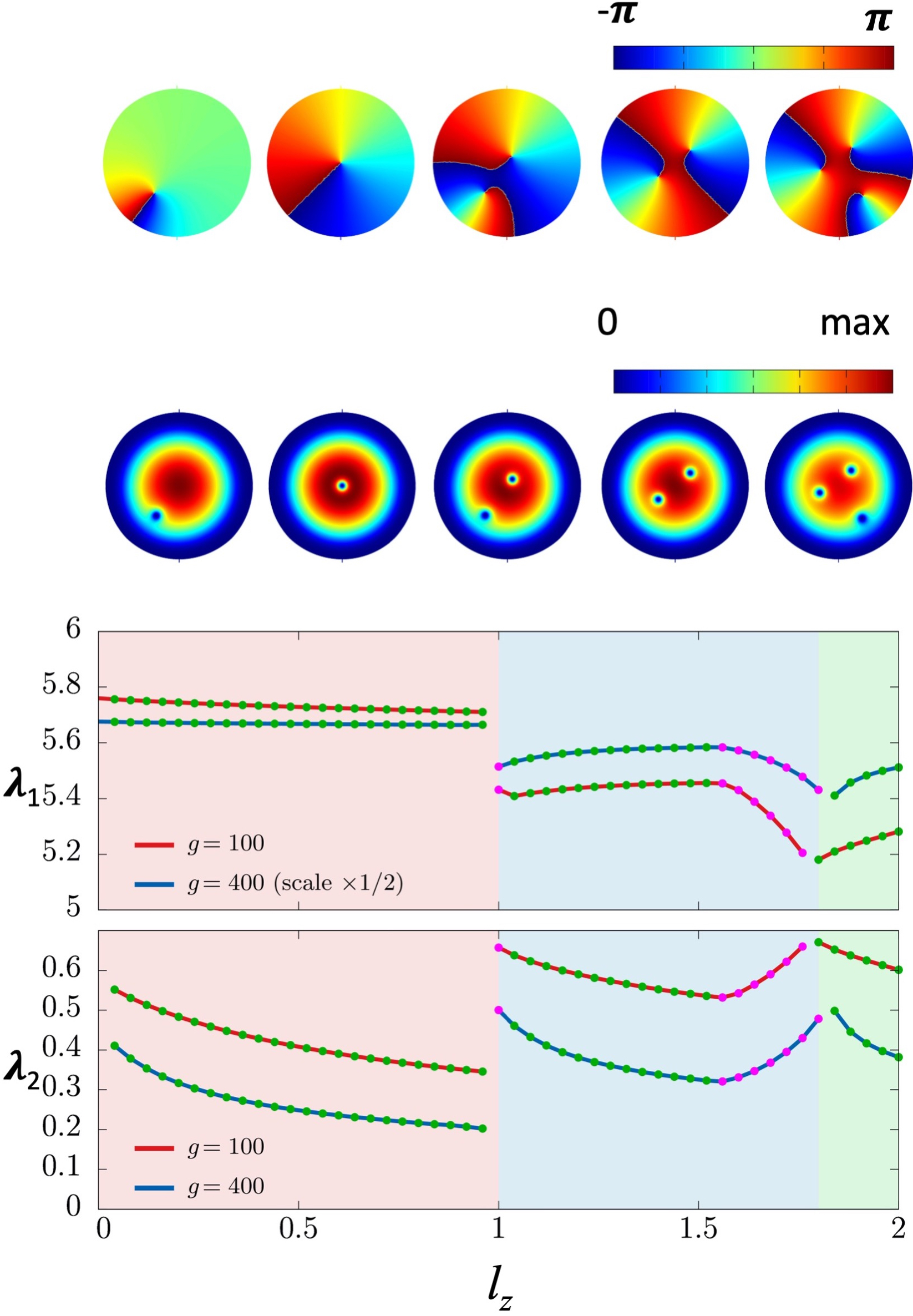
Figure 1: The first line shows the phase of the wave function $\psi^{\star}(\mathbf{x},t)$. The second line shows the density $|\psi^{\star}(\mathbf{x},t)|$ for five representative instantaneous minimum energy vortex solutions of (20), (24): From left to right $0<l_{z}<1.0$, $l_{z}=1$, $0<l_{z}<1.5$, $1.5<l_{z}<1.8$, $1.8<l_{z}<2.0$; the numerical values $1.5,\ 1.8$ are approximative, and depend on the coupling $g$. The vortices rotate around the trap center with angular velocity determined by $\lambda_{2}^{\star}$. In these figures the value of coupling is $g=400$ which is representative for cold atom Bose-Einstein condensates  Garaud-2021a . The bottom panels show the evolution of Lagrange multipliers $\lambda_{1,2}^{\star}$ for $g=100$ and $g=400$.

Remarkably, when $l_{z}\to 0$ neither of these multipliers vanish,

$$\lim_{l_{z}\to 0}\lambda_{1,2}^{\star}(l_{z})\not=0$$ (27)

Since $\lambda_{2}^{\star}$ determines the angular velocity around the trap center (26), this means that for any $l_{z}\not=0,1$ the minimum energy solution describes a rotating vortex configuration.

For $l_{z}=1$ the vortex core coincides with the trap center, only its phase has time dependence. For $l_{z}=0$ the minimum energy solution is a real valued function, up to a constant phase factor. For $0<|l_{z}|<1$ the distance between the vortex core, located at point ${\tt p}\in\mathbb{R}^{2}$, and the trap center increases as $|l_{z}|$ decreases. Notably, the limit $l_{z}\to 0$ is discontinuous and to inspect this I introduce the superfluid velocity

$$\mathbf{v}(\mathbf{x},t)=\nabla\arg[\psi](\mathbf{x},t)$$ (28)

and I define its integer valued circulation

$$i_{\mathbf{v}}({\tt p};\Gamma)\ =\ \frac{1}{2\pi}\oint_{\Gamma}d{\boldsymbol{\ell}}\cdot\mathbf{v}$$ (29)

where $\Gamma$ is a closed trajectory on the plane that does not go thru any singular point of $\mathbf{v}(\mathbf{x},t)$. For any given $l_{z}\not=0$ I can always choose $\Gamma$ to be a circle around the trap center and with a large enough radius, so that the core ${\tt p}$ of a given vortex is inside this circle. For a single vortex the value of (29) is $i_{\mathbf{v}}({\tt p};\Gamma)=\pm 1$, with positive sign for $l_{z}>0$ and negative for $l_{z}<0$. For $l_{z}=0$ the value of the integral (29) vanishes, and for this value the phase of $\psi(\mathbf{x},t)$ can be chosen to vanish; the entire plane is a fixed point of (28) for $l_{z}=0$.

The circulation (29) is an integer valued topological invariant. In particular it can not be continuously deformed as a function of $l_{z}$, when $l_{z}$ varies between $i_{\mathbf{v}}({\tt p};\Gamma)=+1$ for $l_{z}>0$ and $i_{\mathbf{v}}({\tt p};\Gamma)=-1$ for $l_{z}<0$. When $|l_{z}|$ continues to increase to values $|l_{z}|>1$ the value of (29) increases but always in integer steps, as new vortex cores enter inside the (sufficiently large radius) circle $\Gamma$. Thus the vortex structures are topologically protected timecrystalline solutions of (20).

V 5. Timecrystalline molecular chains

I now proceed to a general class of Hamiltonian time crystals. The Hamiltonians describe discrete, piecewise linear chains Dai-2019 ; Dai-2020 . One can think of the vertices $\mathbf{r}_{i}$ ($i=1,...,N$) as point-like interaction centers, they can e.g. model atoms or small molecules in a coarse grained description of a linear polymer. The links $\mathbf{n}_{i}=\mathbf{r}_{i+1}-\mathbf{r}_{i}$ between the vertices then model e.g. the covalent bonds, or peptide planes in the case of a protein chain. For clarity I only consider cyclic chains, with the convention $\mathbf{r}_{N+1}=\mathbf{r}_{1}$.

In an actual molecule, the covalent bonds are very rigid and oscillate rapidly, with a characteristic period as short as a few femtoseconds. I am mostly interested in timecrystalline dynamics at much longer time scales. Thus I assume that the lengths of the links are constant, and equal to their time averaged values in the underlying atomistic system. For simplicity I take all the links to have an equal length with the numerical value

$$|\mathbf{n}_{i}|\equiv|\mathbf{r}_{i+1}-\mathbf{r}_{i}|=1$$ (30)

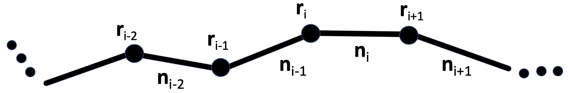
Figure 2: The dynamical variables $\mathbf{n}_{i}=\mathbf{r}_{i+1}-\mathbf{r}_{i}$ are links that connect the vertices $\mathbf{r}_{i}$ of a piecewise linear chain.

The link variables $\mathbf{n}_{i}$ are the dynamical coordinates in my set-up. I subject them to the Lie-Poisson bracket Dai-2019

$$\{n_{i}^{a},n_{j}^{b}\}=\pm\epsilon^{abc}\delta_{ij}n^{c}_{i}$$ (31)

where I can choose either sign on the r.h.s. and for clarity I choose $+$-sign; the two signs are related by parity i.e. change in direction of $\mathbf{n}_{i}$. The bracket is designed to generate all possible local motions of the chain except for stretching and shrinking of its links,

$$\{\mathbf{n}_{i},\mathbf{n}_{k}\cdot\mathbf{n}_{k}\}=0$$

for all pairs ($i,k$), so that (30) is preserved for all times, independently of the Hamiltonian details.

Remarkably, the same bracket (31) appears in Kirchhoff’s theory of a rigid body that moves in an unbounded incompressible and irrotational fluid that is at rest at infinity Milne .

Hamilton’s equation coincides with the Landau-Lifschitz equation

$$\frac{\partial\mathbf{n}_{i}}{\partial t}=\{\mathbf{n}_{i},H\}=\mathbf{n}_{i}\times\frac{\partial H}{\partial\mathbf{n}_{i}}$$ (32)

and the condition that the chain is closed gives rise to the first class constraints

$$\begin{split}&\mathbf{G}\equiv\sum_{i=1}^{N}\mathbf{n}_{i}\ =\ 0\\ &\{G^{a},G^{b}\}=\epsilon^{abc}G^{c}\\ &\{\mathbf{G},H\}=0\end{split}$$ (33)

The last equation restricts the form of Hamiltonian functions I consider. Such Hamiltonians $H_{i}(\mathbf{n})$ can be constructed e.g. as linear combinations of the Hamiltonians that appear in the integrable hierarchy of the Heisenberg chain:

$$\begin{split}H_{1}=&\sum\limits_{i}a_{i}\mathbf{n}_{i}\cdot\mathbf{n}_{i+1}\\ H_{2}=&\sum\limits_{i}b_{i}\mathbf{n}_{i}\cdot(\mathbf{n}_{i-1}\times\mathbf{n}_{i+1})\\ H_{3}=&\sum\limits_{i}c_{i}\mathbf{n}_{i}\cdot(\mathbf{n}_{i-1}\times(\mathbf{n}_{i+1}\times\mathbf{n}_{i+2}))\\ H_{4}=&\sum\limits_{i}d_{i}\mathbf{n}_{i-1}\cdot\mathbf{n}_{i+1}\\ {\it etc.}&\end{split}$$ (34)

where $a_{i},b_{i},c_{i},d_{i}$ are parameters. Furthermore,

$$\mathbf{r}_{i}-\mathbf{r}_{j}=\frac{1}{2}(\mathbf{n}_{j}+...+\mathbf{n}_{i-1}-\mathbf{n}_{i}-...-\mathbf{n}_{j-1})$$ (35)

where I have symmetrized the distance, since there are two ways to connect $\mathbf{r}_{i}$ and $\mathbf{r}_{j}$ along the chain. As a consequence I can also introduce two-body interactions between distant vertices as contributions in a Hamiltonian, such as a combination of electromagnetic Coulomb potential and the Lennard-Jones potential:

$$U(\mathbf{x}_{1},...,\mathbf{x}_{N})=\frac{1}{2}{\sum_{\buildrel i,j=1\over{i\not=j}}^{N}}\frac{e_{i}e_{j}}{|\mathbf{x}_{i}-\mathbf{x}_{j}|}+\frac{\epsilon}{2}{\sum_{\buildrel i,j=1\over{i\not=j}}^{N}}\left\{\left(\frac{\sigma_{P}}{|\mathbf{x}_{i}-\mathbf{x}_{j}|}\right)^{\!\!12}-\left(\frac{\sigma_{vdW}}{|\mathbf{x}_{i}-\mathbf{x}_{j}|}\right)^{\!\!6}\right\}$$ (36)

Here $e_{i}$ is the charge at the vertex $\mathbf{x}_{i}$, $\sigma_{P}$ characterizes the extent of the Pauli exclusion that prevents chain crossing, and $\sigma_{vdW}$ is the range of the van der Waals interaction. All are commonplace in molecular modeling, and in particular they comply with the conditions (33).

Thus, the combination of (34) and (36) can be employed to construct realistic coarse grained Hamiltonian functions $H$ that describe dynamics of (closed) molecular chains, in a way that only depends on the vectors $\mathbf{n}_{i}$.

Note in particular that (33) implies that an initially closed chain remains a closed chain during the time evolution (32).

I follow the general formalism of Section 2 to search for a time crystal as a minimum of $H(\mathbf{n})$ that is subject to the chain closure condition (33). The minimum is a critical point of the following version of (7), (9)

$$\begin{split}&H_{\boldsymbol{\lambda}}=H+{\boldsymbol{\lambda}}\cdot\mathbf{G}\\ &\frac{\partial H}{\partial\mathbf{n}_{i}}_{|\mathbf{n}^{\star}}=-{\boldsymbol{\lambda}}^{\star}\ \ \ \ \ \ \ \&\ \ \ \ \ \mathbf{G}(\mathbf{n}^{\star})=0\\ \Rightarrow\ \ &\frac{\partial H}{\partial t}=\ {\boldsymbol{\lambda}}^{\star}\times\mathbf{n}_{i}\ \ \ \ \ \&\ \ \ \ \ \mathbf{n}_{i}(t=0)=\mathbf{n}_{i}^{\star}\end{split}$$ (37)

Whenever the solution $\boldsymbol{\lambda}^{\star}\not=0$ I have a time crystal as a closed polygonal chain that rotates like a rigid body. The direction of its rotation and its angular velocity are both determined by the direction and the magnitude of the time independent vector $\boldsymbol{\lambda}^{\star}$. Thus, the present timecrystalline Hamiltonian framework provides an effective theory framework for modeling the autonomous dynamics of rotating cyclic molecules.

In practice, to construct the minimum of $H(\mathbf{n})$ I extend (32) to the Landau-Lifschitz-Gilbert equation for $H_{\boldsymbol{\lambda}}$ anton ; Dai-2020

$$\frac{\partial\mathbf{n}_{i}}{\partial t}=-\mathbf{n}_{i}\times\frac{\partial H_{\boldsymbol{\lambda}}}{\partial\mathbf{n}_{i}}+\mu\,\mathbf{n}_{i}\times(\mathbf{n}_{i}\times\frac{\partial H_{\boldsymbol{\lambda}}}{\partial\mathbf{n}_{i}})$$ (38)

with $\mu>0$ the large$-t$ limit is a critical point of $H_{\boldsymbol{\lambda}}$ since (38) gives

$$\frac{dH_{\boldsymbol{\lambda}}}{dt}=-\frac{\mu}{1+\mu^{2}}\sum\limits_{i=1}^{N}\left|\frac{\partial\mathbf{n}_{i}}{\partial t}\right|^{2}$$ (39)

so that the time evolution (38) proceeds towards decreasing values of $H_{\boldsymbol{\lambda}}$ and the flow continues until a critical point ($\mathbf{n}_{i}^{\star}\,,{\boldsymbol{\lambda}}^{\star}$) is reached. Whenever more than one solution exist, I choose the one with smallest value of $H$.

V.1 Simple examples

V.1.1 5.1 Triangular time crystal

The first simple example is an equilateral triangle, with Hamiltonian Dai-2019

$$H=\sum\limits_{i=1}^{3}a_{i}\mathbf{n}_{i}\cdot\mathbf{n}_{i+1}\ +\ b\mathbf{n}_{1}\cdot(\mathbf{n}_{2}\times\mathbf{n}_{3})$$ (40)

Hamilton’s equation (32) gives

$$\begin{split}\partial_{t}\mathbf{n}_{1}\ =\ &\mathbf{n}_{1}\times(a_{1}\mathbf{n}_{2}+a_{3}\mathbf{n}_{3})+b\mathbf{n}_{1}\times(\mathbf{n}_{2}\times\mathbf{n}_{3})\\ \partial_{t}\mathbf{n}_{2}\ =\ &\mathbf{n}_{2}\times(a_{2}\mathbf{n}_{3}+a_{1}\mathbf{n}_{1})+b\mathbf{n}_{2}\times(\mathbf{n}_{3}\times\mathbf{n}_{1})\\ \partial_{t}\mathbf{n}_{3}\ =\ &\mathbf{n}_{3}\times(a_{3}\mathbf{n}_{1}+a_{2}\mathbf{n}_{2})+b\mathbf{n}_{3}\times(\mathbf{n}_{1}\times\mathbf{n}_{2})\end{split}$$ (41)

By summing these equations I obtain

$$\frac{d}{dt}(\mathbf{n}_{1}+\mathbf{n}_{2}+\mathbf{n}_{3})=0$$

This confirms that an initially closed chain remains closed for all $t$. Moreover, for general choice of parameters ($a_{i},b$) the r.h.s. of (41) never vanishes; the minimum of $H$ for a closed chain is not a critical point of $H$; the minimum is time dependent i.e. a time crystal. The time crystal describes rotation with an angular velocity around an axis, with direction determined by the parameters. See Figure 3.

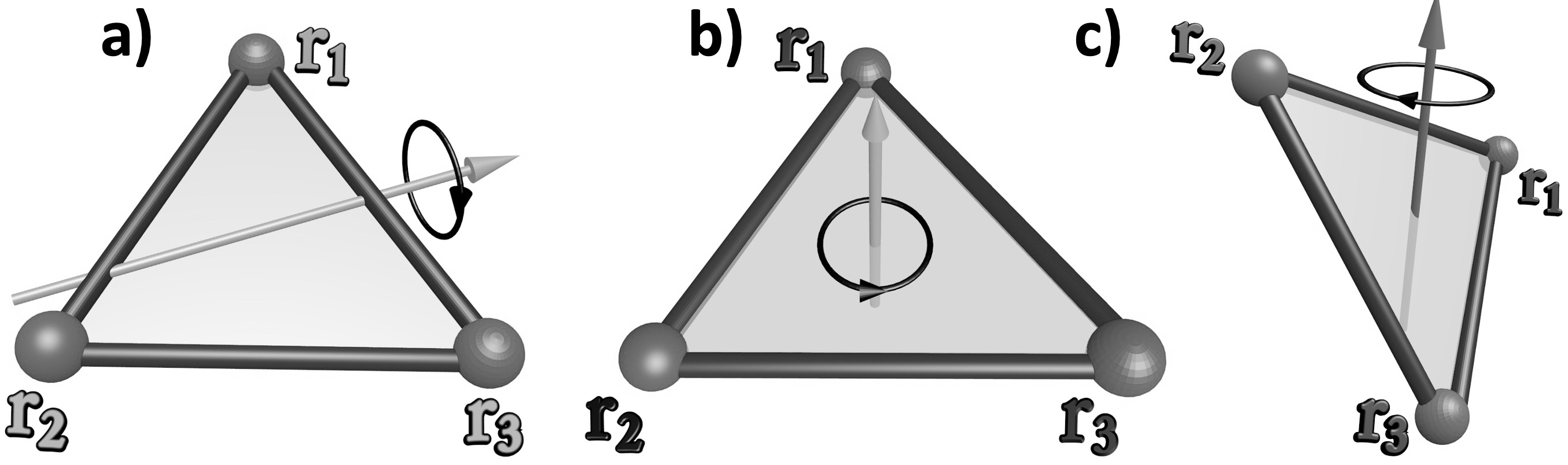
Figure 3: a): A timecrystalline triangle with $b=0$ and rotation axis determined by the $a_{i}$. b): A timecrystalline triangle with $a_{i}=0$, $b\not=0$ and the rotation axis is the symmetric normal to the triangular plane. c): For generic ($a_{i},b$) the rotation axis points to generic direction.

V.1.2 5.2 Knotted time crystals

The second concrete, simple example involves only the long range energy function (36), with Hamiltonian Dai-2020

$$H=\frac{1}{2}{\sum_{\buildrel i,j=1\over{i\not=j}}^{12}\left\{\frac{1}{|\mathbf{r}_{i}-\mathbf{r}_{j}|}\ +\ \left(\frac{3/4}{|\mathbf{r}_{i}-\mathbf{r}_{j}|}\right)^{12}\right\}}$$ (42)

The first term is a Coulomb repulsion between the vertices and the second term is a short range Pauli repulsion that prevents chain crossing; in an actual molecule the covalent bonds can not cross each other. The links connecting the $N=12$ vertices are chosen to have the topology of a trefoil knot. The initial knot geometry is otherwise random. The Hamiltonian is first minimized using the Landau-Lifschitz-Gilbert equation (38). The set-up is an example of (32), (33). The Figure 4 shows the resulting minimum energy time crystal, how it rotates according to (32) around the axis that coincides with the vector ${\boldsymbol{\lambda}}^{\star}$.

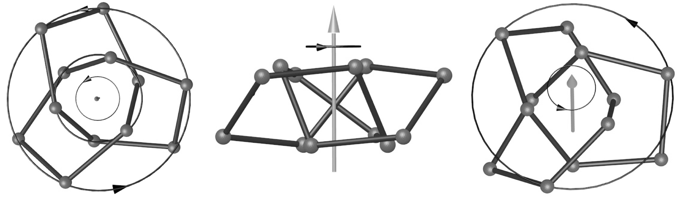
Figure 4: A topological time crystal, with the topology of a trefoil knot, viewed from three different directions. The energy function is given by (42), the rotation axis points in the direction of $\boldsymbol{\lambda}^{\star}$ and the angular velocity is proportional to $|\boldsymbol{\lambda}^{\star}|$.

Various combinations of the local angles (34) and the long distance interactions (36) can be introduced. The ensuing energy functions can describe time crystalline structures, also with more elaborate knot topologies than a trefoil. At a higher level of realism, the interaction centers at the vertices can be given their internal atomic structure. Eventually, one ends up with a highly realistic all-atom molecular dynamics description of a polymer chain, which is the subject of the next Section.

VI 6. Cyclopropane and Sisyphus

VI.1 6.1 Cyclopropane as a time crystal

All-atom molecular dynamics simulations are the most realistic descriptions that are presently available to model chain-like molecules. CHARMM  charmm is an example of such a molecular dynamics energy function, and GROMACS gromacs is a user-friendly package for performing simulations. A typical molecular dynamics energy function contains the following terms; here the summations cover all atoms of the molecule and can also extend e.g. over ambient water molecules.

$$\begin{split}V(\mathbf{x}_{i})&=\sum\limits_{bonds}k_{bi}(l_{i}-l_{i0})^{2}+\sum\limits_{angles}k_{ai}(\theta_{i}-\theta_{i0})^{2}+\sum\limits_{torsions}V_{i}^{n}[1-\cos(n\omega_{i}-\gamma_{i})]\\ &+{\sum_{{i\not=j}}}\left\{\frac{e_{i}e_{j}}{|\mathbf{x}_{i}-\mathbf{x}_{j}|}+\frac{\epsilon_{ij}}{2}\left[\left(\frac{r_{min}}{|\mathbf{x}_{i}-\mathbf{x}_{j}|}\right)^{\!\!12}-2\left(\frac{r_{min}}{|\mathbf{x}_{i}-\mathbf{x}_{j}|}\right)^{\!\!6}\right]\right\}\end{split}$$ (43)

The first term describes the stretching and shrinking of covalent bonds; it is not present in (34), (36) where the Lie-Poisson bracket (31) preserves the bond lengths. The second and third terms account for the bending and twisting in the covalent bonds. These terms are akin quadratic/harmonic approximations to non-linear terms that are listed in (34). The last term is a combination of the electromagnetic and Lennard-Jones interactions (36). There can also be additional terms such as the Urey-Bradley interaction between atoms separated by two bonds (1,3 interaction), and improper dihedral terms for chirality and planarity; these can also be descrobed by the higher order terms in (34). The time evolution is always computed from Newton’s equation, with the force field that derives from (43).

In the case of a molecular chain, a typical characteristic time scale for a covalent bond oscillation that is due to stretching and shrinking of the bond described by the first term in (43), can be as short as a few femtoseconds. In practical observations of molecular motions the time scales are usually much longer, and the observed covalent bond lengths commonly correspond to time averaged values. For the bending and twisting motions the characteristic time scales are much longer than for stretching and shrinking. Thus a separation of scales should take place so that an effective theory description becomes practical. Indeed, many phenomena that are duly consequences of the free energy (43) can often be adequately modeled by an effective theory description. The effective theory energy function can be a combination of terms such as those in (34), (36) and its dynamics can be described by the Lie-Poisson bracket (31), in a useful approximation.

To investigate how the separation of scales takes place, and how an effective theory description emerges, in [ 33] all-atom molecular dynamics has been used to simulate the ground state of an isolated cyclopropane molecule C₃H₆ shown in Figure 5. The force field is CHARMM36m, in combination with GROMACS. The simulation starts with a search of the

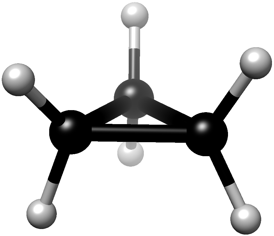
Figure 5:   Cyclopropane C₃H₆ with $D_{3h}$ molecular symmetry.

minimum energy configuration, at a given ultra low internal temperature factor value; very low temperature thermal oscillations could be interpreted as mimicking quantum oscillations in a semiclassical description. The initial atomic coordinates can be found from the PubMed site  PubMed where the positions of the carbon and hydrogen atoms are specified with $10^{-14}\,$m precision. In [ 33] the structure is further optimized so that it describes a local minimum of the CHARMM36m energy function, with full $D_{3h}$ molecular symmetry where the carbon-carbon bond angles are $60^{\mathrm{o}}$ and the hydrogen pairs are in full eclipse. Starting from this energy minimum all-atom trajectories are constructed, to simulate 10$\mu$s of cyclopropane dynamics, at different ultra low internal temperature factor values. The simulations use double precision floating point accuracy and the length of the simulation time step is 1.0$f$s; for the detailed set-up and for simulation details I refer to [ 33]. All the individual atom coordinates are followed and recorded, and analysed at different stroboscopic time steps $\Delta_{s}t$, during the entire 10 $\mu$s molecular dynamics trajectory.

When the cyclopropane is simulated with the very low $\sim 0.067$K internal temperature factor value, and the all the atom positions are observed at every $\Delta_{s}t=100n$s (or longer) stroboscopic time step, the molecule rotates uniformly at constant angular velocity. The axis of rotation coincides with the (time averaged) center of mass axis that is normal to the plane of the three carbon atoms. Remarkably, this stroboscopic rotational motion is identical to the motion of a triangular Hamiltonian time crystal shown in Figure 3 b): The dynamics is described by the generalized Landau-Lifschitz equation (32), with the Hamiltonian $H_{2}$ in (34. The results confirm that the timecrystalline Hamiltonian $H_{2}$ is an effective theory for this stroboscopic motion, in the limit of long stroboscopic time steps.

VI.2 6.2 Spontaneous symmetry breaking

Notably, the Lie-Poisson bracket (31) breaks parity; if the sign on the r.h.s. is changed, the rotation direction in Figure 3) b) also changes. Obviously something similar needs to take place in cyclopropane for it to rotate in a particular direction: The cyclopropane is a priori a highly symmetric molecule with $D_{3h}$ molecular symmetry; the carbon-carbon bond angles are all $60^{\rm o}$ and the dihedrals of all hydrogen pairs are fully eclipsed. In this maximally symmetric state there can not be any unidirectional rotational motion around the molecular symmetry axis that is normal to the plane of carbons, as there is no way to select between clockwise and counterclockwise rotational direction. However, the bond angles are much smaller than the optimum $109.5^{\rm o}$ angles of a normal tetrahedral carbon atom, and there is considerable torsional strain between the fully eclipsed hydrogen pairs strain . Thus one can expect that in the lowest energy ground state the $D_{3h}$ symmetry becomes spontaneously broken. By rigidity of covalent bond lengths I expect that the symmetry breakdown should be mainly due to a twisting of the dihedral angles, between the hydrogen pairs. This spontaneous symmetry breakdown selects a rotation direction, since parity is no longer a symmetry. The simulation results that I have described show that this indeed occurs: The unidirectional rotation around the triangular symmetry axis in the limit of long stroboscopic time steps is a manifestation of broken parity.

A simple model free energy can be introduced, to demonstrate how the spontaneous symmetry breaking due to strain in hydrogen pair dihedral angles can take place. With $\theta_{i}$ ($i=1,2,3$) the dihedrals, the free energy is

$$F(\theta_{1},\theta_{2},\theta_{3})=\frac{1}{4}\sum\limits_{i=1}^{3}g(\theta_{i}^{2}-\alpha^{2})^{4}$$ (44)

The eclipsed configuration with all $\theta_{i}=0$ is a local maximum, and a critical point of the free energy. The minimum of (44) occurs when $\theta_{i}=\pm\alpha$, the value of $\alpha$ corresponds to the optimal value of the dihedral angle for two staggered hydrogen pairs. But in the cyclopropane molecule the three dihedrals are subject to the condition

$$\theta_{1}+\theta_{2}+\theta_{3}=0$$ (45)

Thus $\theta_{i}^{min}=\pm\alpha$ is not achievable for non-vanishing $\alpha$. Instead I need to find the minimum of (44) subject to the condition (45). This is (again) a problem in constrained optimization, so I search for critical points of

$$F_{\lambda}=\frac{1}{4}\sum\limits_{i=1}^{3}g(\theta_{i}^{2}-\alpha^{2})^{4}+\lambda(\theta_{1}+\theta_{2}+\theta_{3})$$

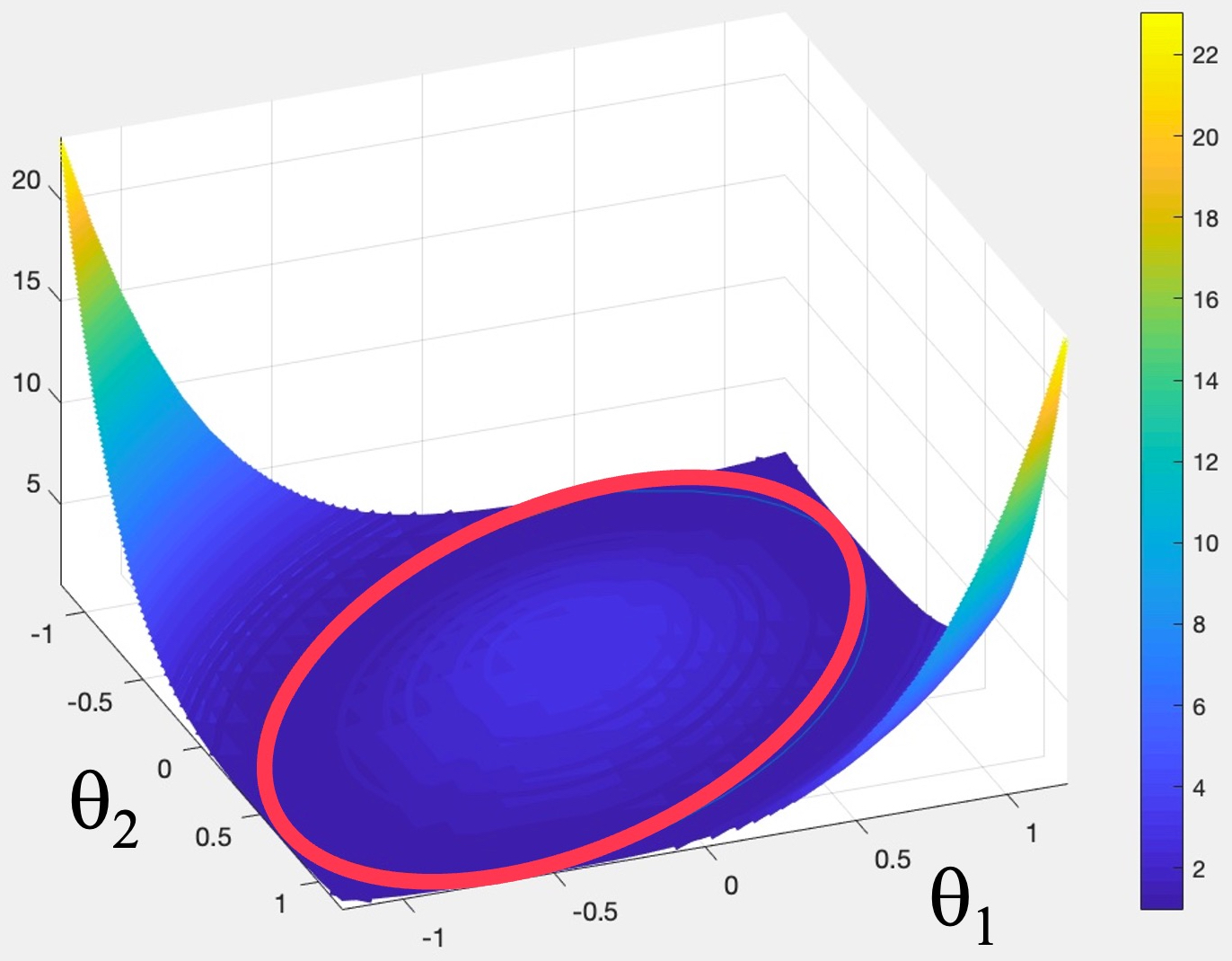
Figure 6:   Free energy (44) with $\theta_{3}$ given by (45), and its minimum.

with $\lambda$ the Lagrange multiplier; I can rescale the angles, and set $a=g=1$ in which case the critical points obey

$$\theta_{i}(\theta_{i}^{2}-1)+\lambda=0$$ (46)

in addition of (45). I eliminate $\theta_{3}$ and plot the minimum of the rescaled (44) as a function of $\theta_{1}$ and $\theta_{2}$. The result is shown in Figure 6. The minimum forms a circular curve on the ($\theta_{1},\theta_{2}$) plane around the origin. In particular, the $D_{3h}$ symmetry becomes spontaneously broken, by the minimum. The Lagrange multiplier can be solved from (46). It is non-vanishing except when $\theta_{1}$ has the value 0 or $\pm 1$ and $\theta_{2}$ is $\pm 1$ or 0, respectively. The non-vanishing of $\lambda$ is suggestive of a time crystal, in line with the general theory of Section 2.

VI.3 6.3 Sisyphus

The Newtonian dynamics with the CHARMM36m force field is much more complex that the generalized Landau-Lifschitz evolution (32) with the Hamiltonian $H_{2}$ in (34). Thus one can not expect that the cyclopropane molecule continues to display the same uniform, timecrystalline rotational motion when one decreases the length of the stroboscopic time step $\Delta_{s}t$. The Figure 7 shows how the rotational motion proceeds as function of the decreasing length of the stroboscopic time step; these Figures display the instantaneous stroboscopic value of the rotation angle $\theta(t)$ around the normal axis of the carbon triangle.

$\bullet~{}$ Figure 7 a) shows the result for $\Delta_{s}t=100n$s, when the effective theory description (32) with the Hamiltonian $H_{2}$ in (34) is accurate: The rotation is uniform, with a constant angular velocity.

$\bullet~{}$ In Figure 7 b) the length of the stroboscopic time step is decreased to $\Delta_{s}t=20\,p$s. There is a very small amplitude ratcheting, with an almost constant amplitude oscillations around the average value of the increasing rotation angle.

$\bullet~{}$ In Figure 7 c) the stroboscopic time step is decreased to $\Delta_{s}t=2.0\,p$s. The amplitude of ratcheting oscillations around the average value of $\theta$ has substantially increased: The molecule turns around regularly and rotates in the opposite direction, but at a slightly smaller relative value of angular velocity $\omega_{s}\equiv\dot{\theta}$. The period of ratcheting oscillations in $\theta(t)$ are also shorter than in Figure 7 b).

$\bullet~{}$ Finally, in Figure 7 d) the molecule is sampled with stroboscopic time steps $\Delta_{s}t=200\,f$s. Now the motion is becoming more chaotic, it consists of a superposition of very rapid back-and-forth rotations with different amplitudes and frequencies, and with only a slow relative drift towards increasing values of $\theta(t)$.

The results shown in Figures 7 demonstrate how the separation of scales takes place in the simulated cyclopropane: There is a continuous, smooth cross-over transition from a large-$\Delta_{s}t$ regime of a uniform timecrystalline rotation, through an intermediate $\Delta_{s}t$ regime with increasingly ratcheting rotational motion, to a small-$\Delta_{s}t$ regime that is dominated by rapid back-and-forth oscillations, with different amplitudes and frequencies. Remarkably, when the stroboscopic time step decreases, the time evolution of the cyclopropane becomes qualitatively increasingly similar to the Sisyphus dynamics reported in [ 22]. Thus, the Sisyphus dynamics appears to provide a microscopic level explanation how timecrystalline effective theory Hamiltonian dynamics emerges, at least in a small molecule such as cyclopropane.

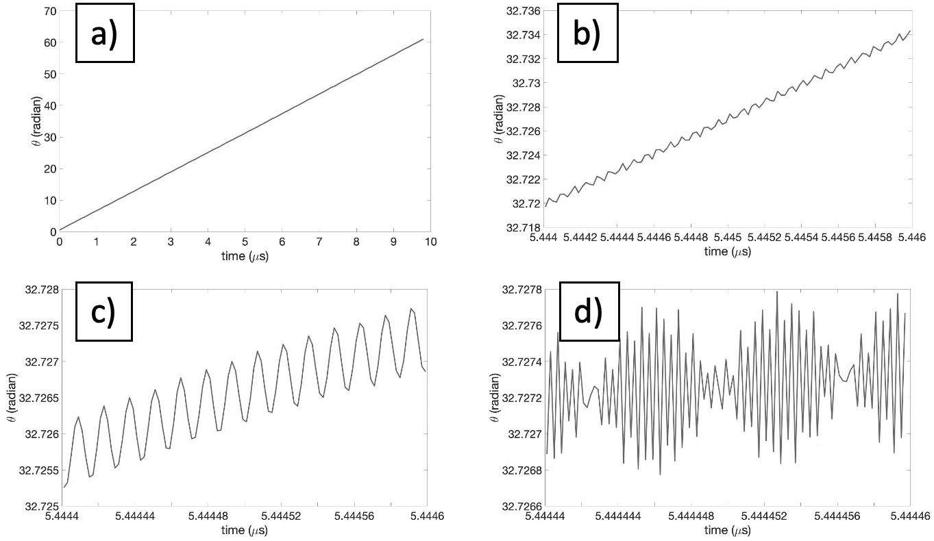
Figure 7: The evolution of the cyclopropane rotation angle during a $10\,\mu$s CHARMM36m simulation and with $T=0.067$K internal temperature factor value, recorded with decreasing stroboscopic time steps: a) The regime of uniform rotation, here with $\Delta_{s}t=100\,n$s. b) and c) describe ratcheting regime, with $\Delta_{s}t=20\,p$s in b) and $\Delta_{s}t=2.0\,p$s in c). Finally d) with $\Delta_{s}t=200\,f$s is in the regime dominated by Sisyphus dynamics.

VII 7. Rotation without angular momentum

Newton’s equation with the CHARMM36m all-atom molecular dynamics force field preserves the angular momentum, and angular momentum is also well preserved in a GROMACS numerical simulation. Since the initial cyclopropane has no angular momentum, the rapid back-and-forth oscillations and in particular the uniform timecrystalline rotational motion that is observed, are in apparent violation of angular momentum conservation. The resolution of the paradox is that the cyclopropane is not a rigid body. It is a deformable body, and a deformable body with at least three movable components can rotate simply by changing its shape Guichardet-1984 ; Shapere-1989b . A falling cat is a good example, how it can maneuver and rotate in air to land on its feet.

In the case of a cyclopropane molecule, when the internal temperature factor has a non-vanishing value, the covalent bonds oscillate so that the shape of the molecule continuously changes; in an actual molecule there are also quantum mechanical zero-point oscillations. Such shape changes are minuscule, but over a long trajectory their effects can accumulate and self-organize into an apparent rotational motion. This is what is described in the Figures 7.

The analysis of results in [ 33] confirm that the angular momentum of the simulated cyclopropane is conserved, and vanishes with numerical precision during the entire $10\,\mu$s simulation trajectory. For this, one evaluates the accumulation of infinitesimal rotations, with each rotation corresponding to that of an instantaneous rigid body. An infinitesimal rigid body rotation can be defined using e.g. Eckart frames, in terms of the instantaneous positions and velocities of all the carbon and hydrogen atoms around the center of mass. In our simulations these are recorded at every $\Delta\tau=10^{-15}\,f$s time step $n$ during the entire $10\,\mu$s production run. The instantaneous values $L(n)$ of the corresponding rigid body angular momentum component along the normal to the instantaneous plane of the three carbon atoms can then be evaluated, together with the corresponding instantaneous moment of inertia values $I(n)$. This gives the following instantaneous “rigid body” angular velocity values

$$\omega(n)=L(n)/I(n)$$

When these are summed up the result is the accumulated “rigid body” rotation angle, at each simulation step $n$:

$$\vartheta(n)=\omega(n)\Delta\tau+\vartheta(n-1)\ =\ \sum\limits_{i=1}^{n}\frac{L(i)}{I(i)}\Delta\tau$$ (47)

In full compliance with the conservation of angular momentum and the vanishing of its initial value, it is found Peng-2021 that in all the $10\,\mu$s production run simulations the accumulated values (47) always remains less than $\sim 10^{-6}$ radians, for all $n$, and the Figure 8 shows a typical example: There is no observable net rotation of the cyclopropane molecule due to “rigid body” angular momentum, with numerical precision. Accordingly any systematic rotational motion that exceeds $\sim 10^{-6}$ radians during a production run simulation must be emergent, and entirely due to shape deformations.

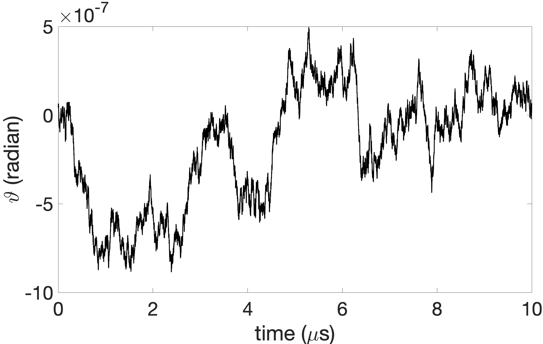
Figure 8: The evolution of the rigid body rotation angle $\vartheta(n)$ in (47), during a typical cyclopropane simulation.

The original articles on rotation by shape deformations are [ 23; 24]. Reviews can be found in [ 25; 18] and here I follow [ 18]: Consider the (time) $t$-evolution of three equal mass point particles that form the corners $\mathbf{r}_{i}$ ($i=1,2,3$) of a triangle. I assume that there are no external forces so that the center of mass does not move,

$$\mathbf{r}_{1}(t)+\mathbf{r}_{2}(t)+\mathbf{r}_{3}(t)=0$$ (48)

for all t. I also assume that the total angular momentum vanishes,

$$\mathbf{L}\ =\ \mathbf{r}_{1}\times\dot{\mathbf{r}}_{1}+\mathbf{r}_{2}\times\dot{\mathbf{r}}_{2}+\mathbf{r}_{3}\times\dot{\mathbf{r}}_{3}\ =\ 0$$ (49)

I now show that nevertheless, the triangle can rotate by changing its shape. To describe this rotational motion, I place the triangle to the $z=0$ plane and with the center of mass at the origin ($x,y$)=($0,0$). Two triangles then have the same shape if they only differ by a rigid rotation on the plane, around the $z$-axis. I can describe shape changes by shape coordinates $\mathbf{s}_{i}(t)$ that I assign to each vertex of the triangle. They describe all possible triangular shapes, in an unambiguous fashion and in particular with no extrinsic rotational motion, when I demand that the vertex $\mathbf{s}_{1}(t)$ always lies on the positive $x$-axis with $s_{1x}(t)>0$ and $s_{1y}(t)=0$, and the vertex $\mathbf{s}_{2}(t)$ has $s_{2y}(t)>0$ but $s_{2x}(t)$ can be arbitrary. The coordinates $\mathbf{s}_{3}(t)$ of the third vertex are then fully determined by the demand that the center of mass remains at the origin:

$$\mathbf{s}_{3}(t)=-\mathbf{s}_{1}(t)-\mathbf{s}_{2}(t)$$

Now, let the shape of the triangle change arbitrarily, but in a $\mathrm{T}$-periodic fashion. As a consequence the $\mathbf{s}_{i}(t)$ evolve also in a $\mathrm{T}$-periodic fashion,

$$\mathbf{s}_{i}(t+T)=\mathbf{s}_{i}(t)$$

as the triangular shape traces a closed loop $\Gamma$ in the space of all possible triangular shapes.

At each time $t$ the shape coordinates $\mathbf{s}_{i}(t)$ and the space coordinates $\mathbf{r}_{i}(t)$ are related by a rotation around the $z=0$ plane,

$$\left(\begin{array}[]{c}r_{ix}(t)\\ r_{iy}(t)\end{array}\right)=\left(\begin{array}[]{cc}\cos\theta(t)&-\sin\theta(t)\\ \sin\theta(t)&\ \cos\theta(t)\end{array}\right)\left(\begin{array}[]{c}s_{ix}(t)\\ s_{iy}(t)\end{array}\right)$$ (50)

Initially $\theta(0)=0$, but if there is any net rotation due to shape changes we have $\theta(\mathrm{T})\not=0$ so that the triangle has rotated during the period, by an angle $\theta(\mathrm{T})$. I substitute (50) into (49) and I get

$$\theta(\mathrm{T})\ \equiv\ \int\limits_{0}^{\mathrm{T}}\!dt\,\frac{d\theta(t)}{dt}\,\ =\ \int\limits_{0}^{\mathrm{T}}\!dt\,\,\frac{\sum\limits_{i=1}^{3}\left\{s_{iy}\dot{s}_{ix}-s_{ix}\dot{s}_{iy}\right\}}{\sum\limits_{i=1}^{3}\mathbf{s}^{2}_{i}}$$ (51)

and in general this does not need to vanish, as I show in the next sub-section

VIII 8. Towards timecrystalline universality

I now evaluate (51) in the case of a time dependent triangular structure, with three point-like interaction centers at the corners. The shape changes are externally driven so that the shape coordinates evolve as follows:

$$\mathbf{s}_{1}(t)\ =\ \frac{1}{\sqrt{3}}\left(\begin{matrix}\cos[a\sin\omega_{1}t]\\ 0\end{matrix}\right)\ \ \ \ \&\ \ \ \ \mathbf{s}_{2}(t)\ =\ \frac{1}{\sqrt{3}}\left(\begin{matrix}\cos[a\sin\omega_{2}t+\frac{2\pi}{3}]\\ \sin(\frac{2\pi}{3})\end{matrix}\right)$$ (52)

I choose $a=0.1$ and $\omega_{2}=2\omega_{1}=3$, substitute in (51) and evaluate the time integral numerically. The Figures 9 a)-d) show how the angle $\theta(t)$ evolves, when observed with different stroboscopic time steps.

When I compare the Figures 7 and 9 I observe a striking qualitative similarity: Except for the scales, the corresponding panels are almost identical.

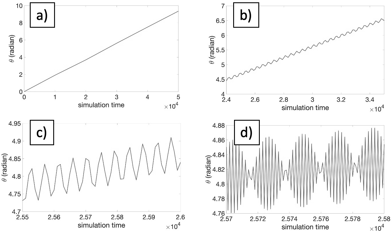
Figure 9: The evolution of the angle $\theta(t)$ of (51) for the shape changes (52), and with stroboscopic time steps. In panel a) $\Delta_{s}t=10^{3}$, In panel b) $\Delta_{s}t=10^{2}$, In panel c) $\Delta_{s}t=10$, and in panel d) $\Delta_{s}t=1$.

In particular, even though the shape changes (52) are externally driven, at large stroboscopic time scales the time evolution again coincides with that of the autonomous Hamiltonian time crystal in Figure 3 b).

The strong qualitative similarity between results in Figure 7 and 9 proposes that the Sisyphus dynamics of [ 22] and the ensuing ratcheting at larger stroboscopic time scales, is akin a universal route, how an oscillatory short time scale stroboscopic evolution becomes self-organized into a Hamiltonian time crystal, at large stroboscopic time scale.

Finally, when I expand the integrand (51), (52) in powers of the amplitude $a$, the result is

$$\frac{d\theta}{dt}\ =\ -\frac{1}{2}\omega_{2}a\cos\omega_{2}t+\frac{\sqrt{3}}{12}a^{2}\left\{\omega_{2}\sin 2\omega_{2}t-\omega_{1}\sin 2\omega_{1}t\right\}-\frac{1}{8}\omega_{2}a^{3}\cos 3\omega_{2}t$$

$$+\frac{1}{16}\omega_{2}a^{3}\left\{\cos(\omega_{2}+2\omega_{1})t+\cos(\omega_{2}-2\omega_{1})t\right\}+{\mathcal{O}}(a^{4})$$ (53)

Thus, exactly when $\omega_{2}=\pm 2\omega_{1}$ will the large time limit of the rotation angle $\theta(t)$ increase linearly in time as follows,

$$\theta(t)\ \buildrel{{\rm large}-t}\over{\longrightarrow}\ \frac{1}{16}\,\omega_{2}a^{3}t$$ (54)

in line with Figure 9 a). But when $\omega_{2}\not=\pm 2\omega_{1}$ the large-$T$ limit of the integral (51) vanishes, by Riemann’s lemma. Similar high sensitivity of the rotation angle is also observed in the case of the cyclopropane, where the role of the parameter $a$ is played by the internal temperature factor of the molecule.

IX Concluding remarks

The concept of a time crystal has made a long journey. It started as a beautiful idea that was soon ridiculed as a fantasy. From there it has progressed to the frontline of theoretical physics research, with high expectations for remarkable future applications. But the notion is still very much under development. The conceptual principles are still under debate and remain to be finalized, there are several parallel and alternative lines of research to follow. The present article describes only my own personal way, how I try to understand what is a time crystal. My interest in the subject started from discussions with Frank, and I am only able to describe what I have learned myself, by doing things on my own, with Frank, and with my close colleagues. There is undoubtedly much that I have not covered, but I leave it to others who know things better.

X Acknowledgements

I thank Anton Alekseev, Jin Dai, Julien Garaud, Xubiao Peng and Frank Wilczek for collaboration on various aspects of the original work described here. My research is supported by the Carl Trygger Foundation Grant CTS 18:276 and by the Swedish Research Council under Contract No. 2018-04411 and by Grant No. 0657-2020-0015 of the Ministry of Science and Higher Education of Russia. I also acknowledge COST Action CA17139.

XI Personal recollections

I conclude with a short personal recollection of the remarkable way how Betsy and Frank have ended up, to spend part of their time in Sweden and Stockholm University.

I first met Betsy and Frank personally in Aspen, during the summer 1984 session. Incidentally, we overlapped there with Michael Green and John Schwarz, during the time when they gave birth to the modern string theory. At that time Frank and I shared a more modest interest, and we discussed certain ideas around the SU(3) Skyrme model. Unfortunately my self-confidence at the time was not at a level, to meet his challenges.

After Aspen we met several times, including Santa Barbara, Cambridge, Uppsala, Tours, Stockholm and elsewhere, not to forget their lovely summer house in New Hampshire. Our discussions were always very enjoyable. Frank even included me in his official delegation to attend the events during the Nobel Week, when he received the 2004 Physics Prize.

In 2007, around the time when Nordita was moving to Stockholm, Frank told me that he had plans for a sabbatical. I succeeded in attracting him to spend half a year in Sweden, jointly between Nordita and my Department at Uppsala University. The other half of his sabbatical he spent at Oxford University, where I also visited him. There, he told me about his dream to walk across the Great Britain. Apparently he hatched the first, very early ideas of a time crystal during this walk. I now regret I did not ask to join him.

While in Uppsala, Frank and I got the idea to organize a Nobel Symposium in graphene. The Symposium took place in Summer 2010, only a few months before the discovery of graphene was awarded the Physics Nobel Prize: Ours was the first ever Nobel Symposium that took place the same year the Prize was awarded on the subject of a Symposium. I understand that the many great talks, walks and discussions during the Symposium helped to decide who got the Prize. Two years later, I hosted Frank when he became honorary doctor at Uppsala University. A little later Frank came back to Uppsala, this time to collect Nobel chocolates that he won from a bet with Janet Conrad, on the discovery of the Higgs boson.

Both Betsy and Frank seemed very happy with their sabbatical stay, and with all other experiences they had at Stockholm and Uppsala. So I started to talk with Frank about the idea, that they could spend a little longer time in Sweden, on a regular basis. In particular, I told Frank that the Swedish Research Council had occasional calls on a funding program for International Recruitments, with very generous conditions. In 2014 the opportunity raised: Soon after the Nobel Symposium on topological insulators at Högberga where Frank gave the summary talk, I learned that the call was again being opened, and that this was probably the last call in the program. I contacted Frank, now with more determination. He was at least lukewarm, so I proposed my colleagues at Uppsala University that we should make an application to try and recruit Frank. Initially, I received several very positive, in fact some enthusiastic, replies from my colleagues at the Department of Physics and Astronomy. But then came one strongly negative reply, from Maxim Zabzine who at the time was responsible for the administration of theoretical physics. Maxim stated that he did not want Uppsala University to make any effort, whatsoever, to apply for a Research Council grant for Frank.

I did not see any point to try and change Maxim’s strong opinion, in particular since the deadline for the application was approaching. Instead, I immediately contacted Lars Bergström at Stockholm University. I asked him if Stockholm University would be willing to submit an application to the Research Council, on Frank’s behalf. I reckon that I contacted Lars only two days before the Nobel Prize of Physics 2014 was announced. Lars was at the time the Permanent Secretary of the Nobel Physics Committee and for sure he had his hands full in preparing the announcement. However, already the next day I received a reply from Anders Karlhede, then Vice President of Stockholm University. Anders wrote that my proposal had been discussed with the President of Stockholm University Astrid Söderberg Widding, and that Stockholm University is delighted to submit an application to the Research Council.

Soon after the Nobel Prize in Physics 2014 was announced and Lars became more free, he and Anders started to work on the formal application; I understand they were also joined by Katherine Freese who was then Director of Nordita. At that time I were in China with Frank. Frank was on his first-ever trip to China, and I coordinated the visits in Beijing together with Vincent Liu. From Beijing we all continued to Hangzhou for the memorable inaugural events of Wilczek Quantum Center at Zhejiang Institute of Technology.

During our travel in China I had several long discussions with Frank about the Research Council grant application. He had his doubts, and I made my best to persuade him. I remember vividly the decisive discussion: After a breakfast at our hotel, a historic place that used to be Mao Zedong’s favorite retreat at the West Lake in Hangzhou, Frank and I were sitting together in the lobby. In Stockholm, the Research Council application was ready to be submitted, the deadline was only a couple of days away. But Stockholm University still needed Frank to sign a formal letter of interest for the application, and Frank was hesitant. However, after some lengthy discussion I got his signature, and I sent the signed letter right away to Anders. In two months time we received a decision from the Research Council that Stockholm University’s application for the International Recruitement Grant for Frank had been approved.

However, it was too early to call it a home run. For that, I still needed some advice from Anders Bárány, who is the creator of Nobel Museum. Anders came up with the brilliant idea, of a curator position for Betsy at Nobel Museum. To launch this, I teamed up with Gérard Mourou who invited Frank and Betsy, and a delegation from Nobel Museum, to the Symposium on Fresnel, Art and Light at Louvre in Paris. Frank gave a beautiful talk, and Betsy made contacts with Louvre art curators. With a strong support from Astrid and Anders things worked out impressively for Betsy at the Nobel Museum, where her achievements included the extraordinary Feynman Exhibition at ArtScience Museum of Marina Bay in Singapore 2018-2019 that she largely organized with Frank’s support and great help from K K Phua. With some additional aid and support from here and there, including Grand hospitality by Katherine Freese at a right time in summer 2015, and in particular with the consistent and very strong support from Astrid and Anders, Betsy and Frank were finally convinced to try and start their present journey in Stockholm. I am really grateful that I can follow and share so much of it with them.

- (1) F. Wilczek, Phys. Rev. Lett. 109 160401 (2012)
- (2) A. Shapere, F. Wilczek, Phys. Rev. Lett. 109 160402 (2012)
- (3) P. Bruno, Phys. Rev. Lett. 111 070402 (2013)
- (4) H. Watanabe, M. Oshikawa, Phys. Rev. Lett. 114 251603 (2015)
- (5) N. Yamamoto, Phys. Rev. D92 085011 (2015)
- (6) K. Sacha, Phys. Rev. A91 033617 (2015)
- (7) K. Sacha, D. Delande, Phys. Rev. A94 023633 (2016)
- (8) V. Khemani, A. Lazarides, R. Moessner, S.L. Sondhi, Phys. Rev. Lett. 116 250401 (2016)
- (9) D.V. Else, C. Nayak, Phys. Rev. B93 201103 (2016)
- (10) D.V. Else, B. Bauer, C. Nayak Phys. Rev. Lett. 117 090402 (2016)
- (11) D. V. Else, B. Bauer, C. Nayak, Phys. Rev. X7 011026 (2017)
- (12) N. Y. Yao, A. C. Potter, I.-D. Potirniche, A. Vishwanath, Phys. Rev. Lett. 118 030401 (2017)
- (13) J. Zhang et.al. Nature 543 217 (2017)
- (14) S. Choi et.al. Nature 543 221 (2017)
- (15) J. Rovny, R. L. Blum, S. E. Barrett, Phys. Rev. Lett. 120 180603 (2018).
- (16) J. Dai, A.J. Niemi, X. Peng, F. Wilczek Phys. Rev. A99 023425-9 (2019)
- (17) A. Alekseev, J. Dai, A.J. Niemi JHEP 08 035 (2020)
- (18) X. Peng, J. Dai, A.J. Niemi, New J. Phys. 22 085006 (2020)
- (19) R. Fletcher, Practical Methods of Optimization. (Wiley, Chichester New York, 1987)
- (20) J. Nocedal and S. J. Wright, Numerical Optimization, Springer Series in Operations Research. (Springer, Heidelberg, 1999)
- (21) J.E. Marsden and T.S. Ratiu, Introduction to Mechanics and Symmetry A Basic Exposition of Classical Mechanical Systems Second Edition (Springer Verlag, New York, 1999)
- (22) A. D. Shapere, F. Wilczek Proc. Natl. Acad. Sci. U.S.A. 116 18772 (2019)
- (23) A. Guichardet, Ann. l’Inst. Henri Poincaré 40 329 (1984)
- (24) A. Shapere, F. Wilczek, Am. J. Phys. 57 514 (1989)
- (25) RG Littlejohn, RG Reinsch, Rev. Mod. Phys. 69 213 (1997)
- (26) E. B. Sonin, Dynamics of Quantised Vortices in Superfluids (Cambridge University Press, Cambridge, 2016).
- (27) J. Garaud, J. Dai, A.J. Niemi, JHEP 2021 7 (2021)
- (28) F. Wilczek, Phys.Rev.Lett. 48 1144 (1982)
- (29) F. Wilczek, Phys.Rev.Lett. 49 957 (1982)
- (30) L. M. Milne-Thomson, Theoretical Hydrodynamics 5th edition (Dover, New York, 1996)
- (31) J Huang et.al., Nature Meth. 14 71 (2017)
- (32) http://manual.gromacs.org/
- (33) X. Peng, J. Dai, A.J. Niemi, New J. Phys. 23 073024 (2021)
- (34) https://pubchem.ncbi.nlm.nih.gov/compound/6351
- (35) V. Dragojlovic, Chem. Texts 1 14 (2015)