An explanation of experimental data of $(g-2)_{e,\mu}$ in 3-3-1 models with inverse seesaw neutrinos

Abstract

We show that the anomalous magnetic moment experimental data of muon and electron $(g-2)_{\mu,e}$ can be explained simultaneously in simple extensions of the 3-3-1 models consisting of new heavy neutrinos and a singly charged Higgs boson. The heavy neutrinos generate active neutrino masses and mixing through the general seesaw mechanism. They also have non-zero Yukawa couplings with singly charged Higgs bosons and right-handed charged leptons, which result in large one-loop contributions known as chirally-enhanced ones. Numerical investigation confirms a conclusion indicated previously that these contributions are the key point to explain the large $(g-2)_{\mu,e}$ data, provided that the inverse seesaw mechanism is necessary to allow both conditions that heavy neutrino masses are above few hundred GeV and non-unitary part of the active neutrino mixing matrix must be large enough.

I Introduction

Recently, anomalous magnetic moments (AMM) of charged leptons $a_{e_{a}}\equiv(g-2)_{e_{a}}/2$ have been studied widely because the recent experimental data shows large deviations from the Standard Model (SM) predictions. The recent improved AMM value of muon $a_{\mu}$ predicted by the SM is accepted widely as Aoyama:2020ynm $a^{\mathrm{SM}}_{\mu}=116591810(43)\times 10^{-11}$, which is derived from the combination of various contributions using the dispersion approach Davier:2010nc ; Davier:2017zfy ; Keshavarzi:2018mgv ; Colangelo:2018mtw ; Hoferichter:2019mqg ; Davier:2019can ; Keshavarzi:2019abf ; Kurz:2014wya ; Melnikov:2003xd ; Masjuan:2017tvw ; Colangelo:2017fiz ; Hoferichter:2018kwz ; Gerardin:2019vio ; Bijnens:2019ghy ; Colangelo:2019uex ; Colangelo:2014qya ; Blum:2019ugy ; Aoyama:2012wk ; Aoyama:2019ryr ; Czarnecki:2002nt ; Gnendiger:2013pva . However, this results is inconsistent with the lattice-QCD calculation Borsanyi:2020mff , which is closer to the recent experimental data. In our work, we will use the larger discrepancy between theoretical and experimental results, because it is more interesting for theoretical discussions and the allowed regions of parameter space are still applicable for the smaller deviation reported in Ref. Borsanyi:2020mff . The latest experimental measurement has been reported from Fermilab Abi:2021gix and is also in agreement with previous experimental result measured by Brookhaven National Laboratory (BNL) E82 Muong-2:2006rrc . A combination of these results in the new average value of $a^{\mathrm{exp}}_{\mu}=116592061(41)\times 10^{-11}$, which leads to the improved standard deviation of 4.2 $\sigma$ from the SM prediction, namely

$$\Delta a^{\mathrm{NP}}_{\mu}\equiv a^{\mathrm{exp}}_{\mu}-a^{\mathrm{SM}}_{\mu}=\left(2.51\pm 0.59\right)\times 10^{-9}\,.$$ (1)

The recent experimental AMM values of electron $a_{e}$ were reported from different groups Hanneke:2008tm ; Parker:2018vye ; Morel:2020dww (for calculation of $a_{e}$ in the SM, see Refs. Aoyama:2012wj ; Aoyama:2012wk ; Laporta:2017okg ; Aoyama:2017uqe ; Terazawa:2018pdc ; Volkov:2019phy ; Gerardin:2020gpp ). In our numerical discussion, we adopt the experimental values of $a_{e}$ corresponding to the following standard deviation of $2.5\sigma$ from the SM one:

$$\Delta a^{\mathrm{NP}}_{e}\equiv a^{\mathrm{exp}}_{e}-a^{\mathrm{SM}}_{e}=\left(-8.7\pm 3.6\right)\times 10^{-13}.$$ (2)

Many models beyond the SM (BSM) have been constructed to explain the experimental data of $(g-2)_{\mu,e}$, such as models adding vector-like lepton multiplets Dermisek:2013gta ; Crivellin:2018qmi ; Escribano:2021css ; Hernandez:2021tii ; Crivellin:2021rbq ; Dermisek:2021ajd ; Chun:2020uzw ; Frank:2020smf ; Endo:2020tkb ; Cogollo:2020nrc ; Chen:2020tfr ; Bharadwaj:2021tgp , leptoquarks Crivellin:2020tsz , both neutral and charged Higss bosons as $SU(2)_{L}$ singlets Mondal:2021vou , $SU(2)_{L}$ triplets of leptons and scalars Arbelaez:2020rbq . The minimal supersymmetric standard model can explain both $(g-2)_{e,\mu}$ data in the regions of the parameter space with light slepton masses below a few hundred GeVs Badziak:2019gaf ; Li:2021koa . Some two Higgs doublet models (THDM) adding new $SU(2)_{L}$ Higgs doublets can give large two-loop contributions to $\Delta a_{\mu}$ Li:2020dbg ; DelleRose:2020oaa ; Botella:2020xzf ; Han:2018znu ; Han:2021gfu , provided that the masses of the new neutral and/or charged Higgs bosons must be light at a few hundred GeVs.

In this work, we will focus on the AMM problems predicted by a BSM class called as 3-3-1 models, constructed based on the $SU(3)_{C}\times SU(3)_{L}\times U(1)_{X}$ group Singer:1980sw ; Pisano:1992bxx ; Frampton:1992wt ; Foot:1992rh ; Pleitez:1992xh ; Foot:1994ym ; Ozer:1995xi ; Diaz:2004fs ; Buras:2012dp ; Hue:2015mna ; Fonseca:2016tbn . It was shown that the early 3-3-1 versions cannot predict large $\Delta a_{\mu}$ given by the experimental data Ky:2000ku ; Kelso:2014qka ; Binh:2015jfz ; DeConto:2016ith ; deJesus:2020upp ; deJesus:2020ngn ; Lindner:2016bgg . Extended versions were introduced to solve this problem, such as 3-3-1 models with new vector-like leptons or inert $SU(3)_{L}$ Higgs triplets  deJesus:2020ngn ; deJesus:2020upp , the models with new singly charged Higgs couplings with heavy neutrinos generating neutrino masses through the inverse seesaw (ISS) mechanism Hue:2020wnn ; Hue:2021xap , and 3-3-1 models with discrete symmetries containing a rather large number of new particles needed to explain the hierarchy problems of fermion masses CarcamoHernandez:2019lhv ; CarcamoHernandez:2020pxw . In Ref. Crivellin:2018qmi , the very precise analytic formulas applicable to calculate general one-loop contributions to AMM in a wide class of BSM were presented. Using these formulas, we can estimate again the previous results available in all current 3-3-1 models. These analytic formulas are consistent with those calculated previously for 3-3-1 models Lavoura:2003xp ; Hue:2017lak . More importantly, we will show that the 3-3-1 models can give large one-loop contributions to AMM by adding new $SU(3)_{L}$ singlets such as singly charged Higgs bosons $h^{\pm}$ and heavy neutrinos, a similar way that was applied to the 3-3-1 model with right-handed (RH) neutrinos (331RHN). On the other hand, Higgs triplets and their Yukawa couplings needed to generate masses for charged leptons, quarks, and neutrinos in many 3-3-1 models may have different features from those in the 331RHN, leading to new predictions of the allowed regions of parameter space satisfying the AMM experimental data predicted by different 3-3-1 models. Heavy neutrinos are needed to generate active neutrino masses and mixing through the general seesaw (GSS) mechanism, and Yukawa couplings of singly charged Higgs boson and RH charged leptons. Hence the new particles result in Yukawa terms like $N\left(\lambda^{L}P_{L}+\lambda^{R}P_{L}\right)e_{a}H^{+}$ corresponding to the presence of the so called chirally-enhanced one-loop contributions proportional to $\lambda^{L*}\lambda^{R}$, where $N$ and $H^{+}$ denote two physical states of a neutrino and a singly charged Higgs boson. They are the most important terms that can be large enough to explain the recent AMM data Crivellin:2018qmi . Other chirally-enhanced one-loop contributions originating from the 3-3-1 models will be also mentioned. For convenience, the 3-3-1 models discussed in our work will be generalized in the form of the 3-3-1 model with an arbitrary parameter $\beta$ (331$\beta$) defining the electric charge operator as follows  Diaz:2004fs ; Buras:2012dp :

$$Q=T_{3}+\beta T_{8}+X.$$ (3)

We have introduced the $SU(3)$ generators $T_{a}$, $a=1,\ldots 8$ and $X$ is the new quantum charge corresponding to the group $U(1)_{X}$. Thus, the charge operator $Q$ depends on two parameters $\beta$ and $X$. The 3-3-1 models corresponding to different $\beta$ distinguish each other by new heavy leptons and quarks arranged in the third components of fermion (anti-)triplets, for example, $\beta=-\sqrt{3},\;\frac{1}{\sqrt{3}},\;-\frac{1}{\sqrt{3}},$ and $0$ for the minimal 3-3-1 model Pisano:1992bxx , the 331RN Foot:1994ym , with heavy singly charged leptons Ozer:1995xi , and the simplest 3-3-1 model Hue:2015mna , respectively. These models result in distinguishable consequences for many interesting processes CarcamoHernandez:2005ka ; Buras:2014yna ; Buras:2016dxz ; Buras:2015kwd ; Long:2018fud . Hence, successful solutions for AMM problems in 3-3-1 models will guarantee their realities.

The explanation of AMM data in Refs. Hue:2020wnn ; Hue:2021xap was just valid for the specific 331RHN model corresponding to $\beta=\pm\frac{1}{\sqrt{3}}$, which results in a special case that heavy $SU(3)_{L}$ leptons in the third components of the lepton (anti) triplets are exotic heavy neutrinos $\psi_{aL}\sim(e_{a},\nu_{a},N_{a})^{T}_{L}$. They play roles of right-handed neutrinos $N_{aR}\equiv(N_{aL})^{c}$, and mix with SM neutrinos through a very special form of the total antisymmetric $3\times 3$ neutrino Dirac mass matrix $m_{D}$. As a result, strict relations between parameters are necessary to explain simultaneously all neutrino oscillation data, AMM $(g-2)_{\mu}$, and constraints of lepton flavor violating (cLFV) decays $e_{b}\to e_{a}\gamma$ that must be consistent with experiments. In addition, the 331RHN model needs three more neutrino singlets for generating the ISS neutrino mass matrix (331ISS), and a singly charged scalar singlet to give large one-loop contributions to AMM of muon, while the destructive interference among different one-loop contributions gives a small total one loop contribution to every decay amplitude $e_{b}\to e_{a}\gamma$.

The models 331$\beta$ and 331ISS need three $SU(3)_{L}$ Higgs triplets for generating non-zero masses of all quarks and leptons at the tree level, including active Dirac and Majorana neutrino masses. Two of these Higgs triplets give masses for SM fermions and gauge bosons, therefore they play the same role as the ones well-known in the two Higgs doublet models. They contain two neutral Higgs components with two vacuum expectation values (VEVs) denoted as $v_{1,2}$ satisfying $v_{1}^{2}+v_{2}^{2}\simeq(246\;\mathrm{GeV})^{2}$. The important parameter $t_{\beta}\equiv v_{2}/v_{1}$, where $v_{2}$ is always chosen to generate the top quark mass, must have a lower bound $t_{\beta}\geq 0.33$ from the perturbative limit of the top quark Yukawa coupling. In the 331ISS model, charged lepton masses and the neutrino Dirac mass term are originated from $v_{1}$, therefore large $t_{\beta}>30$ is the necessary condition to give large one-loop contributions to AMM of muon consistent with experimental data Hue:2021xap . In contrast, the neutrino Dirac mass term comes from the Yukawa couplings of the neutral Higgs component with VEV $v_{2}$ in the 331$\beta$ model. The same property also happens for the Yukawa couplings between leptons and the singly charged Higgs bosons. In addition, no $SU(3)_{L}$ neutral leptons are available, therefore the 331$\beta$ model needs six exotic neutrino singlets for the ISS mechanism. Therefore, the allowed regions of the parameter space give large one-loop contributions to $(g-2)_{e,\mu}$ cannot be generalized qualitatively from previous results given in Ref. Hue:2021xap , which requires large $t_{\beta}$. A first derivation may start from the most important property that the Yukawa couplings of singly charged Higgs singlet and $m_{D}$ relate to the Higgs triplet containing VEV $v_{2}$ instead of $v_{1}$. Therefore, the proper values of $t_{\beta}$ may be small enough to explain the experimental AMM data, leading to the existence of an upper bound for $t_{\beta}$. This may be conflict with the perturbative limit $t_{\beta}\geq 0.33$. This problem will be addressed in this work.

Before coming to detailed analysis, we emphasize our works is helpful because of the following reasons. First, we will see that the $331\beta$ model considered in this work explain simultaneously both experimental data of $(g-2)_{e,\mu}$ only when the mixing between $h^{\pm}$ and singly charged components of the $SU(3)_{L}$ Higgs triplets is non-zero. This non-zero mixing implies the existence of a non-trivial coupling of $h^{\pm}$ with two $SU(3)_{L}$ Higgs triplets, $f_{h}\left(\rho^{\dagger}\eta h^{+}+\mathrm{h.c.}\right)$, which was not introduced previously. This may be an indirect link between $SU(3)_{L}$ Higgs triplets and the ISS neutral lepton singlets, apart from the small ISS mixing among $X_{aR}$ and $\nu_{bL}$. In other words, the existence of the $SU(3)_{L}$ Higgs triplet components can be detected through their decays to leptons. The second reason, many previous discussions on 3-3-1 models showed clearly that they did not accommodate the $(g-2)_{\mu}$ data unless adding some other new particles, such as vector-like fermions,…. Our qualitative estimation in this work provides another interesting approach to confirm this conclusion. Finally, the original appearance of the 3-3-1 models solved some interesting questions, such as the answer to the question of three fermion flavors confirmed by experiments, …. New improved versions of 3-3-1 models have been introduced to explain successfully the latest experimental results. Our model is one of them constructed to explain dark matter data, the hierarchies problems of fermion masses,…Many of them contain complicated particle contents including new singly charged Higgs scalars and neutral leptons. Our discussion on AMM data with a very simple Higgs sector will be helpful for further realization solutions for AMM data in these models.

Our work is arranged as follows. In Sec. II, the 331$\beta$ model will be reviewed, where we pay attention to the leptons, gauge bosons, and Higgs sectors, giving all physical states as well as the couplings that may give large one-loop contributions to AMM. In Sec. III, the $331\beta$ model with the GSS will be presented along with the two particular frameworks of the minimal seesaw (MSS) and simple ISS. In Sec. IV, analytic formulas for one-loop contributions to AMM are constructed. Numerical discussions for both MSS and ISS will be shown in detail. Our main results are collected in Sec. V. There are three appendices listing master functions for one-loop contributions to AMM given in Ref. Crivellin:2018qmi , analytic formulas for one-loop contributions from the singly charged Higgs bosons to AMM, and a detailed discussion on the masses and mixing of the singly charged bosons.

II The 3-3-1 model with arbitrary $\beta$

Let us review the $331\beta$ model. Left-handed leptons are assigned to anti-triplets and RH leptons are singlets:

$$L^{\prime}_{aL}=\left(\begin{array}[]{c}e^{\prime}_{a}\\ -\nu^{\prime}_{a}\\ E^{\prime}_{a}\\ \end{array}\right)_{L}\sim\left(3^{*}~{},-\frac{1}{2}+\frac{\beta}{2\sqrt{3}}\right),\hskip 14.22636pta=1,2,3,$$ (7)

$$e^{\prime}_{aR}\sim\left(1~{},-1\right),\hskip 14.22636ptX_{IR}\sim\left(~{}1~{},0\right),\hskip 14.22636ptE^{\prime}_{aR}\sim\left(~{}1~{},-\frac{1}{2}+\frac{\sqrt{3}\beta}{2}\right).$$ (8)

The model includes $K$ RH neutrinos $X_{IR}$, $I=1,2,...,K$, and three exotic leptons $E^{\prime a}_{L,R}$ which are much heavier than the normal leptons. The prime denotes flavor states to be distinguished with mass eigenstates introduced later. The numbers in the parentheses are to label the representation of $SU(3)_{L}\otimes U(1)_{X}$ group. The quark sector is ignored here because it is irrelevant to our present work. We note that our result will be true for 3-3-1 models consisting left-handed lepton triplets because they are equivalent with the models with lepton sector defined in Eq. (8) through a transformation keeping physical results unchanged Descotes-Genon:2017ptp ; Hue:2018dqf .

The model has nine electroweak gauge bosons, included in the following covariant derivative

$$D_{\mu}\equiv\partial_{\mu}-igT^{a}W^{a}_{\mu}-ig_{X}XT^{9}X_{\mu},$$ (9)

where $T^{9}=1/\sqrt{6}$, $g$ and $g_{X}$ are gauge couplings of the two groups $SU(3)_{L}$ and $U(1)_{X}$, respectively. The matrix $W^{a}T^{a}$, where $T^{a}=\lambda_{a}/2$ corresponding to a triplet representation, is written as

$$W^{a}_{\mu}T^{a}=\frac{1}{2}\left(\begin{array}[]{ccc}W^{3}_{\mu}+\frac{1}{\sqrt{3}}W^{8}_{\mu}&\sqrt{2}W^{+}_{\mu}&\sqrt{2}Y^{A}_{\mu}\\ \sqrt{2}W^{-}_{\mu}&-W^{3}_{\mu}+\frac{1}{\sqrt{3}}W^{8}_{\mu}&\sqrt{2}V^{B}_{\mu}\\ \sqrt{2}Y^{-A}_{\mu}&\sqrt{2}V^{-B}_{\mu}&-\frac{2}{\sqrt{3}}W^{8}_{\mu}\\ \end{array}\right),$$ (13)

where we have defined the mass eigenstates of the charged gauge bosons as

$$W^{\pm}_{\mu}=\frac{1}{\sqrt{2}}\left(W^{1}_{\mu}\mp iW^{2}_{\mu}\right),$$

$$Y^{\pm A}_{\mu}=\frac{1}{\sqrt{2}}\left(W^{4}_{\mu}\mp iW^{5}_{\mu}\right),$$

$$V^{\pm B}_{\mu}=\frac{1}{\sqrt{2}}\left(W^{6}_{\mu}\mp iW^{7}_{\mu}\right).$$ (14)

From Eq. (3), the electric charges of the gauge bosons are calculated as

$$A=\frac{1}{2}+\frac{\sqrt{3}\beta}{2},\quad B=-\frac{1}{2}+\frac{\sqrt{3}\beta}{2}.$$ (15)

To generate masses for gauge bosons and fermions, the model has three scalar triplets defined as

$$\chi=\left(\begin{array}[]{c}\chi_{A}\\ \chi_{B}\\ \chi^{0}\\ \end{array}\right)\sim\left(3~{},\frac{\beta}{\sqrt{3}}\right),\hskip 14.22636pt\rho=\left(\begin{array}[]{c}\rho^{+}\\ \rho^{0}\\ \rho^{-B}\\ \end{array}\right)\sim\left(3~{},\frac{1}{2}-\frac{\beta}{2\sqrt{3}}\right)$$ (22)

$$\eta=\left(\begin{array}[]{c}\eta^{0}\\ \eta^{-}\\ \eta^{-A}\\ \end{array}\right)\sim\left(3~{},-\frac{1}{2}-\frac{\beta}{2\sqrt{3}}\right),\;h^{+}\sim(1,1,1).$$ (26)

where $A,B$ denote electric charges as defined in Eq. (15); and $h^{+}$ is a new singly charged Higgs boson needed for giving large one-loop contributions to AMM. These Higgs bosons develop the following non-zero VEVs

$$\langle\chi^{0}\rangle=\frac{u}{\sqrt{2}},\;\langle\rho^{0}\rangle=\frac{v_{2}}{\sqrt{2}},\;\langle\eta^{0}\rangle=\frac{v_{1}}{\sqrt{2}}.$$ (27)

This VEV configuration of the $331\beta$ model without $h^{\pm}$ was shown to be valid in Ref. Costantini:2020xrn . This is also true for the $331\beta$ adding new singly charged Higgs boson $h^{\pm}$ we consider here. For convenience, we will use the following notations:

$$t_{\beta} \equiv\frac{v_{2}}{v_{1}},\;\rightarrow s_{\beta}=\frac{v_{2}}{v},\;c_{\beta}=\frac{v_{1}}{v},$$ (28)

where $v^{2}\equiv v_{1}^{2}+v_{2}^{2}$, and $s^{2}_{\beta}+c^{2}_{\beta}=1$.

The symmetry breaking happens in two steps: $SU(3)_{L}\otimes U(1)_{X}\xrightarrow{u}SU(2)_{L}\otimes U(1)_{Y}\xrightarrow{v_{1},v_{2}}U(1)_{Q}$, leading to the condition that $u\gg v_{1},v_{2}$. After the first step, five gauge bosons will be massive and the remaining four massless ones can be identified with the before-symmetry-breaking SM gauge bosons, resulting in the following important equation:

$$\frac{g_{X}^{2}}{g^{2}}=\frac{6s_{W}^{2}}{1-(1+\beta^{2})s_{W}^{2}},\;g=g_{2},$$ (29)

where the weak mixing angle is defined as $t_{W}=\tan\theta_{W}=g_{1}/g_{2}$, $g_{1,2}$ are the gauge couplings of the SM gauge groups $U(1)_{Y}$ and $SU(2)_{L}$, respectively. We denote $s_{W}=\sin\theta_{W}$ and $c_{W}=\cos\theta_{W}$. Putting in the value of $s_{W}$, we get approximately

$$|\beta|\leq\sqrt{3}.$$ (30)

The masses of the charged gauge bosons are

$$m^{2}_{Y^{\pm A}}=\frac{g^{2}}{4}(u^{2}+v^{2}_{1}),\quad m^{2}_{V^{\pm B}}=\frac{g^{2}}{4}(u^{2}+v^{2}_{2}),\quad m^{2}_{W^{\pm}}=\frac{g^{2}}{4}(v^{2}_{1}+v^{2}_{2}),$$ (31)

where the gauge boson $W^{\pm}$ is identified with the SM one, implying that

$$v^{2}\equiv v_{1}^{2}+v_{2}^{2}=\frac{4m_{W}^{2}}{g^{2}}\simeq(246\;\mathrm{GeV})^{2}.$$ (32)

The above Higgs bosons are enough to generate all SM quark masses and heavy new quark masses Buras:2012dp ; Hung:2019jue . In addition, the Yukawa term $Y^{u}_{3a}\overline{Q_{3L}}\rho^{*}u_{aR}\to\frac{Y^{u}_{3a}v_{2}}{\sqrt{2}}\overline{u_{3L}}u_{aR}$ mainly contributes to the top quark mass, $m_{t}\simeq\frac{Y^{u}_{33}v_{2}}{\sqrt{2}}\leq\sqrt{4\pi}v_{2}/\sqrt{2}$, equivalently $s_{\beta}\geq\sqrt{2}m_{t}/(\sqrt{4\pi}v)\to t_{\beta}\geq 0.3$.

In general, the mixing between a SM lepton and a new lepton is allowed if they have the same electric charge in some particular values of $\beta$. This mixing effect will be neglected in the $331\beta$ model under consideration. The Yukawa Lagrangian now is

$$-\mathcal{L}^{\text{yuk}}_{\mathrm{lepton}} =Y^{e}_{ab}\overline{e^{\prime}_{aR}}\eta^{T}L^{\prime}_{bL}+Y^{E}_{ab}\overline{E^{\prime}_{aR}}\chi^{T}L^{\prime}_{bL}+Y^{X}_{Ib}\overline{X_{IR}}\rho^{T}L^{\prime}_{bL}+\frac{1}{2}M_{N,IJ}\overline{X_{IR}}(X_{JR})^{c}$$

$$+Y^{h}_{Ib}\overline{(X_{IR})^{c}}e^{\prime}_{bR}h^{+}+\mathrm{h.c.},$$ (33)

where $a,b=1,2,3$ are family indices, and $I=1,2,3,...K$ are the number of new neutral lepton singlets. The perturbative limit of the $Y^{h}$ is important in this work, which should satisfy $|Y^{h}_{Ia}|<\sqrt{4\pi}$. In fact, the trust values of $|Y^{h}_{Ia}|$ may be smaller Allwicher:2021rtd . In Lagrangian (II), the neutrino Dirac mass matrix comes from the third term including the Higgs triplet $\rho$ which also generates the top quark mass. This important property is different from that given in Ref. Hue:2021xap , hence the dependence of the Dirac mass term, the Yukawa couplings of singly charged Higgs bosons, and the perturbative condition of the Yukawa couplings with heavy neutrinos $Y^{X}_{Ib}$ on $t_{\beta}$ will be different between two models 331$\beta$ and 331ISS discussed in Ref. Hue:2021xap . In later discussions, we will set $K=3$ and $K=6$ for the respective MSS and ISS mechanisms considered in this work. The corresponding mass terms are:

$$-\mathcal{L}^{\text{mass}}_{\mathrm{lepton}} =\frac{Y^{e}_{ab}v_{1}}{\sqrt{2}}\overline{e^{\prime}_{aR}}e^{\prime}_{bL}+\frac{Y^{E}_{ab}u}{\sqrt{2}}\overline{E^{\prime}_{aR}}E^{\prime}_{bL}$$

$$+\frac{1}{2}\begin{pmatrix}\overline{(\nu^{\prime}_{L})^{c}}&\overline{X_{R}}\end{pmatrix}\mathcal{M}^{\nu}\begin{pmatrix}\nu^{\prime}_{L}\\ (X_{R})^{c}\end{pmatrix}+\mathrm{h.c.},\mathcal{M}^{\nu}=\begin{pmatrix}0_{3\times 3}&M^{T}_{D}\\ M_{D}&M_{N}\end{pmatrix}\;,$$ (34)

where $(M_{D})_{Ib}\equiv M_{D,Ib}=\frac{-Y^{X}_{Ib}v_{2}}{\sqrt{2}}$, $\nu^{\prime}_{L}=(\nu^{\prime}_{1},\nu^{\prime}_{2},\nu^{\prime}_{3})_{L}^{T}$ and $X_{R}=(X_{1},X_{2},...,X_{K})_{R}^{T}$. Note that, here, charged lepton masses and $M_{D}$ come from different Higgs triplets, while these mass terms discussed in Ref. Hue:2021xap come from the same Higgs triplet. Therefore, the effects on $\Delta a_{\mu,e}$ relating to the relevant Yukawa couplings in the model under consideration will be different from those discussed in Ref. Hue:2021xap . At present, the active neutrino masses and mixing are still generated from the GSS mechanism. The total mixing matrix is defined as

$$U^{\nu T}\mathcal{M}^{\nu}U^{\nu} =\hat{\mathcal{M}}^{\nu}=\mathrm{diag}(m_{n_{1}},\;m_{n_{1}},\;...,m_{n_{K+3}}),$$

$$\begin{pmatrix}\nu^{\prime}_{L}\\ (X_{R})^{c}\end{pmatrix} =U^{\nu}n_{L},\;\begin{pmatrix}(\nu^{\prime}_{L})^{c}\\ X_{R}\end{pmatrix}=U^{\nu*}n_{R}=U^{\nu*}(n_{L})^{c},\;$$ (35)

where $n_{L,R}=(n_{1},n_{2},...,n_{(K+3)})_{L,R}$ are Majorana neutrino mass eigenstates satisfying $n_{iL,R}=(n_{iR,L})^{c}$, and the four-component forms are $n_{i}=(n_{iL},n_{iR})^{T}$.

From now on we will work in the basis where the SM charged leptons are in their mass eigenstates, namely $Y^{e}_{ab}=Y^{e}_{ab}\delta_{ab}$ and $e^{\prime}_{a}=e_{a}$ in Eqs. (II) and (34). This can always be done without loss of generality. The transformations from the flavor states to mass eigenstates of the heavy lepton $E_{a}$ are defined as

$$E^{\prime}_{aL}=V^{L}_{ab}E_{bL},\quad E^{\prime}_{aR}=V^{R}_{ab}E_{bR},$$ (36)

where $V^{L,R}$ is a $3\times 3$ unitary mixing matrix for new charged leptons.

For the Higgs sector, the ratios between VEVs are used to define two mixing angles:

$$s^{2}_{iu}=\sin^{2}\beta_{iu}=\frac{v_{i}^{2}}{u^{2}+v_{i}^{2}},\;i=1,2.$$ (37)

We will also use the following notations $t_{iu}=s_{iu}/c_{iu}$. The scalar potential is

$$V_{\mathrm{h}} =\mu_{1}^{2}\eta^{\dagger}\eta+\mu_{2}^{2}\rho^{\dagger}\rho+\mu_{3}^{2}\chi^{\dagger}\chi+\lambda_{1}\left(\eta^{\dagger}\eta\right)^{2}+\lambda_{2}\left(\rho^{\dagger}\rho\right)^{2}+\lambda_{3}\left(\chi^{\dagger}\chi\right)^{2}$$

$$+\lambda_{12}(\eta^{\dagger}\eta)(\rho^{\dagger}\rho)+\lambda_{13}(\eta^{\dagger}\eta)(\chi^{\dagger}\chi)+\lambda_{23}(\rho^{\dagger}\rho)(\chi^{\dagger}\chi)$$

$$+\tilde{\lambda}_{12}(\eta^{\dagger}\rho)(\rho^{\dagger}\eta)+\tilde{\lambda}_{13}(\eta^{\dagger}\chi)(\chi^{\dagger}\eta)+\tilde{\lambda}_{23}(\rho^{\dagger}\chi)(\chi^{\dagger}\rho)$$

$$+\sqrt{2}f\left(\epsilon_{ijk}\eta^{i}\rho^{j}\chi^{k}+\mathrm{h.c.}\right)$$

$$+\mu_{4}^{2}h^{+}h^{-}+f_{h}\left(\rho^{\dagger}\eta h^{+}+\mathrm{h.c.}\right)+(h^{+}h^{-})\left(\lambda^{h}_{1}\eta^{\dagger}\eta+\lambda^{h}_{2}\rho^{\dagger}\rho+\lambda^{h}_{3}\chi^{\dagger}\chi\right)+\lambda^{h}_{4}\left(h^{+}h^{-}\right)^{2},$$ (38)

where the last line includes all terms relating to the singly charged Higgs boson that does not appear in the previous versions Diaz:2004fs ; Buras:2012dp . The triple coupling $f_{h}$ is a very important parameter controlling the mixing between the singly charged Higgs components of the two $SU(3)_{L}$ Higgs triplets and the Higgs singlet $h^{\pm}$. It is emphasized that the existence of $f_{h}$ is a very interesting feature of the 331$\beta$ that did not mention previously, because of the nontrivial property that the coupling $\rho^{\dagger}\eta h^{+}$ always respects $U(1)_{X}$ symmetry for arbitrary $\beta$.

As we mentioned above, the VEV configuration considered in this work is the same as that chosen in Refs. Costantini:2020xrn ; DeConto:2015eia , which was shown to be consistent with the unitarity, perturbativity and bounded-from-below (BFB) constraints. On the other hand, the exact necessary and sufficient BFB constraints are still difficult to determine Faro:2019vcd . They relate to the copositive (conditionally positive) conditions of the quartic term of the Higgs potential to guarantee the existence of local minima, as discussed in ref. Kannike:2012pe . Determining which local minimum is the global one defining the stability of the Higgs potential corresponding to the VEV structure chosen in this work is more difficult. A method introduced in ref. Maniatis:2006fs can solve this problem, but it is still difficult to apply to BSM models with complicated Higgs sectors such as the 3-3-1 models. The discussions on the VEV structure mentioned in Refs. Costantini:2020xrn ; DeConto:2015eia were not addressed clearly to the vacuum stability issue. In the model under consideration, the global minimum corresponding to the VEV structure mentioned above requires more relations between Higgs couplings. We hope that the large number of Higgs couplings appearing in the Higgs potential (38) will allow the existence of these new relations consistent with the available constraints. They should be discussed in more detail when the Higgs phenomenology is focused. It is not our scope in this work, we therefore will not discuss more.

A detailed calculation to derive masses and mixing matrix of the singly charged Higgs bosons is shown in appendix C. From this, the relations between the mass and flavor eigenstates of singly charged Higgs bosons are

$$\begin{pmatrix}\rho^{\pm}&\\ \eta^{\pm}&\\ h^{\pm}&\end{pmatrix} =\begin{pmatrix}-s_{\beta}&c_{\alpha}c_{\beta}&s_{\alpha}c_{\beta}\\ c_{\beta}&c_{\alpha}s_{\beta}&s_{\alpha}s_{\beta}\\ 0&-s_{\alpha}&c_{\alpha}\end{pmatrix}\begin{pmatrix}\phi_{W}^{\pm}&\\ H_{1}^{\pm}&\\ H_{2}^{\pm}&\end{pmatrix},$$ (39)

where $\phi_{W}^{\pm}$ are the Goldstone bosons of $W^{\pm}$, $H^{\pm}_{1,2}$ are two physical states with masses $m_{H^{\pm}_{1,2}}$, and $\alpha$ is a new mixing parameter defined in Eq. (149). Normally, $m_{H^{\pm}_{1,2}}$ and $\alpha$ are functions of the potential couplings. For convenience, we will consider $\alpha$, and $m_{H^{+}_{1,2}}$ as free parameters, while $\mu_{4}$, $f$, and $f_{h}$ are chosen as functions of all free ones, namely:

$$\mu^{2}_{4} =c^{2}_{\alpha}m^{2}_{H^{\pm}_{2}}+s^{2}_{\alpha}m^{2}_{H^{\pm}_{1}}-\frac{1}{2}\left(\lambda^{h}_{1}s^{2}_{\beta}v^{2}+\lambda^{h}_{2}c^{2}_{\beta}v^{2}+\lambda^{h}_{3}u^{2}\right),$$

$$f =-\frac{c_{\beta}s_{\beta}\left(-\tilde{\lambda}_{12}v^{2}+2c_{\alpha}^{2}m_{H_{1}^{\pm}}^{2}+2s_{\alpha}^{2}m_{H_{2}^{\pm}}^{2}\right)}{2u},$$

$$f_{h} =-\frac{\sqrt{2}s_{\alpha}c_{\alpha}\left(m^{2}_{H^{\pm}_{1}}-m^{2}_{H^{\pm}_{2}}\right)}{v}.$$ (40)

The case of $s_{\alpha}=0$ or $c_{\alpha}=0$ will return to the decouple limit between $h^{\pm}$ and the $SU(3)_{L}$ Higgs triplets mentioned in Ref. Hue:2021xap , where this limit is allowed. In contrast, we will see that $s_{2\alpha}=2s_{\alpha}c_{\alpha}\neq 0$, equivalently, the triple Higgs coupling $f_{h}\neq 0$, is one of the necessary condition to give large one-loop contributions to AMM in the $331\beta$.

The relations between the mass and flavor eigenstates of other charged Higgs bosons are:

$$\left(\begin{array}[]{c}\eta^{\pm A}\\ \chi^{\pm A}\\ \end{array}\right) =\left(\begin{array}[]{cc}s_{1u}&c_{1u}\\ -c_{1u}&s_{1u}\\ \end{array}\right)\left(\begin{array}[]{c}\phi^{\pm A}_{Y}\\ H^{\pm A}\\ \end{array}\right),\;\left(\begin{array}[]{c}\rho^{\pm B}\\ \chi^{\pm B}\\ \end{array}\right)=\left(\begin{array}[]{cc}s_{2u}&-c_{2u}\\ c_{2u}&s_{2u}\\ \end{array}\right)\left(\begin{array}[]{c}\phi^{\pm B}_{V}\\ H^{\pm B}\\ \end{array}\right),$$ (53)

where $\phi_{W}^{\pm}$, $\phi^{\pm A}_{Y}$ and $\phi^{\pm B}_{V}$ are the Goldstone bosons of $W^{\pm}$, $Y^{\pm A}$ and $V^{\pm B}$, respectively. The masses of the charged Higgs bosons $H^{\pm A},H^{\pm B}$ are

$$m^{2}_{H^{A}}=(u^{2}+v_{1}^{2})\left(\frac{-fv_{2}}{v_{1}u}+\frac{1}{2}\tilde{\lambda}_{13}\right),\;m^{2}_{H^{B}}=(u^{2}+v^{2}_{2})\left(\frac{-fv_{1}}{uv_{2}}+\frac{1}{2}\tilde{\lambda}_{23}\right).$$ (54)

Because the neutral Higgs bosons couple to charged lepton through the Yukawa couplings of the form $S^{0}\overline{e_{a}}e_{a}$, which is the same form as that of the SM-like Higgs boson predicted by the SM, the corresponding one-loop contributions to AMM is very small. Hence, they will be ignored in our calculation from now on. The discussion on the identification of the SM-like Higgs boson can be found in Ref. Hung:2019jue . In total, there are six charged Higgs bosons, one neutral pseudoscalar Higgs and three neutral scalar Higgs bosons.

III The minimal seesaw and inverse seesaw mechanisms in the neutral lepton sector

In this section, we will collect important properties of the MSS and ISS mechanisms used in our calculation. In the GSS framework, the neutrino mixing matrix is parameterized in the following form:

$$U^{\nu}=\left(\begin{array}[]{cc}\left(I_{3}-\frac{1}{2}RR^{\dagger}\right)U_{\mathrm{PMNS}}&RV\\ -R^{\dagger}U_{\mathrm{PMNS}}&\left(I_{K}-\frac{1}{2}R^{\dagger}R\right)V\\ \end{array}\right)+\mathcal{O}(R^{3}),$$ (55)

where $V$ is a $K\times K$ unitary matrix; $R$ is a $3\times K$ matrix satisfying $|R_{aI}|<1$ for all $a=1,2,3$, and $I=1,2,...,K$. The $3\times 3$ unitary matrix $U_{\mathrm{PMNS}}$ is the Pontecorvo-Maki-Nakagawa-Sakata (PMNS) matrix ParticleDataGroup:2020ssz . The GSS relations are

$$R \simeq M^{\dagger}_{D}{M^{*}_{N}}^{-1},\;m_{\nu}\simeq-M^{T}_{D}M_{N}^{-1}M_{D}=U^{*}_{\mathrm{PMNS}}\hat{m}_{\nu}U^{\dagger}_{\mathrm{PMNS}},$$

$$V^{*}\hat{M}_{N}V \simeq M_{N}+\frac{1}{2}R^{T}R^{*}M_{N}+\frac{1}{2}M_{N}R^{\dagger}R,$$ (56)

where $\hat{m}_{\nu}=\mathrm{diag}(m_{n_{1}},m_{n_{1}},m_{n_{3}})$ and $\hat{M}_{N}=\mathrm{diag}(m_{n_{4}},m_{n_{5}},...,m_{n_{(K+3)}})$ consist of three active neutrino and $K$ new heavy neutrino masses, respectively. In many formulas discussed below, we will use the equality that $\left(\hat{m}_{\nu}\right)_{cc}=m_{n_{c}}$ with $c=1,2,3$ are active neutrino masses.

The general parameterization of $M_{D}$ was introduced in Ref. Casas:2001sr . In the limit of the MSS mechanism with $K=3$, we will use the simplest forms of $M_{N}$ and $M_{D}\equiv m_{D}$ as follows Arganda:2014dta ; Ibarra:2010xw ,

$$M_{N}=M_{0}I_{3},\;M_{D}\equiv m_{D}=i\sqrt{M_{0}\hat{m}_{\nu}}U^{\dagger}_{\mathrm{PMNS}}.$$ (57)

The relations in (56) reduce to the following simple form:

$$R=-iU_{\mathrm{PMNS}}\left(\frac{\hat{m}_{\nu}}{M_{0}}\right)^{1/2},\quad V\simeq I_{3},\quad\hat{M}_{N}\simeq M_{N},\;m_{n_{4,5,6}}\simeq M_{0}.$$ (58)

In the ISS mechanism with $K=6$, the total neutrino mixing matrix $U^{\nu}$ in (55) is $9\times 9$. In the 331$\beta$ model, the well-known ISS form of the total neutrino matrix can be derived from the requirement that the model respects a global $U(1)_{\mathcal{L}}$ symmetry called the generalized lepton number, which is defined from the following formula: $\mathcal{L}$: $L\equiv-\frac{4}{\sqrt{3}}T^{8}+\mathcal{L}$, where $L$ is the normal lepton number defined in the SM that $L(\ell)=1$ for all SM leptons $\ell=e,\mu,\tau,\nu_{eL},\nu_{\mu L},\nu_{\tau L}$ and zero for all other SM particles including quarks, gauge, and Higgs bosons Tully:2000kk ; Chang:2006aa ; CarcamoHernandez:2017cwi . The specific $\mathcal{L}$ assignments for all Higgs bosons and fermions in two 3-3-1 models with right-handed neutrinos and the minimal ones in Refs. Tully:2000kk ; Chang:2006aa ; CarcamoHernandez:2017cwi are the same and independent with $\beta$, therefore they are valid for the 331$\beta$ model with $\mathcal{L}(L^{\prime}_{aL})=1/3$, $\mathcal{L}(e^{\prime}_{aR})=1$. In addition, introducing $\mathcal{L}(\rho)=\mathcal{L}(\eta)=2/3$, $\mathcal{L}(\chi)=-4/3$, $\mathcal{L}(h^{+})=0$, and $\mathcal{L}(E^{\prime}_{aR})=-1$ will result in the Lagrangian (II) conserving $\mathcal{L}$, except the mass term $\overline{X_{IR}}(X_{JR})^{c}$, which includes soft-breaking terms. Namely, choosing that $\mathcal{L}(X_{IR})=1$ with $I\leq 3$ and $\mathcal{L}(X_{IR})=-1$ with $I>3$, the conserved Lagrangian (II) implies that $Y^{h}=\left(\mathcal{O}_{3\times 3},\;Y^{h}_{2}\right)^{T}$ and $Y^{X}=\left(Y^{X}_{1},\;\mathcal{O}_{3\times 3}\right)^{T}$, where $Y^{h}_{2}$, and $Y^{X}_{1}$ are two $3\times 3$ matrices, and $\mathcal{O}_{3\times 3}$ is the $3\times 3$ null matrix. This leads to the ISS form of $M_{D}=(m_{D},\;\mathcal{O}_{3\times 3})^{T}$. The $6\times 6$ Majorojana mass matrix $M_{N}$ consists of three parts denoted as $M_{R}$, $\mu_{X}$, and $\mu^{\prime}_{X}$. The conserved mass term $\left(M_{R}\right)_{ab}\equiv M_{N,a(b+3)}$ with $a,b\leq 3$ can be arbitrary large, while the soft-breaking term $\left(\mu^{\prime}_{X}\right)_{ab}\equiv M_{N,ab}$ and $\left(\mu_{X}\right)_{ab}\equiv M_{N,(a+3)(b+3)}$ should be small. Inserting the ISS form of $M_{D}$ into the GSS relations to derive the active neutrino mass term $m_{\nu}$, we find that small $\mu^{\prime}_{X}$ does not affect significantly the final result. Hence, we assume the simplest case of $\mu^{\prime}_{X}=\mathcal{O}_{3\times 3}$ without loss of generality.

Now, the Dirac and Majorana mass matrices have well-known ISS forms as follows Arganda:2014dta ; Ibarra:2010xw

$$M^{T}_{D}=(m^{T}_{D},\hskip 14.22636pt\mathcal{O}_{3\times 3}),\hskip 14.22636ptM_{N}=\left(\begin{array}[]{cc}\mathcal{O}_{3\times 3}&M_{R}\\ M^{T}_{R}&\mu_{X}\\ \end{array}\right).$$ (61)

Defining $M=M_{R}\mu_{X}^{-1}M_{R}^{T}$, the ISS relations now are

$$R =M^{\dagger}_{D}{M^{*}_{N}}^{-1}=\left(-m_{D}^{\dagger}M^{*-1},\hskip 14.22636ptm^{\dagger}_{D}\left(M^{\dagger}_{R}\right)^{-1}\right),$$

$$m_{\nu} =-M^{T}_{D}M_{N}^{-1}M_{D}=m_{D}^{T}\left(M_{R}^{T}\right)^{-1}\mu_{X}M_{R}^{-1}m_{D},$$

$$V^{*}\hat{M}_{N}V^{\dagger} \simeq M_{N}+\frac{1}{2}R^{T}R^{*}M_{N}+\frac{1}{2}M_{N}R^{\dagger}R.$$ (62)

In the ISS framework, $m_{D}$ is parameterized in terms of many free parameters, hence it is enough to choose $\mu_{X}=\mu_{X}I_{3}$. The parameter $\mu_{X}$ is a new scale making the most important difference between the neutrino mixing matrices in the ISS and MSS. We also assume that $M_{R}=\hat{M}_{R}=M_{0}I_{3}$. A simple parameterization of $m_{D}$ is $m_{D}=\mathrm{diag}(\sqrt{M_{11}},\;\sqrt{M_{22}},\;\sqrt{M_{33}})\sqrt{\hat{m}_{\nu}}U^{\dagger}_{\mathrm{PMNS}}$ Arganda:2014dta , which is completely different from the total antisymmetric $m_{D}$ given in Ref. Hue:2021xap . The ISS condition $|\hat{m}_{\nu}|\ll|\mu_{X}|\ll|m_{D}|\ll M_{0}$ gives $\frac{\sqrt{\mu_{X}\hat{m}_{\nu}}}{M_{0}}\simeq 0$. Then we have

$$\hat{M}_{N}=\left(\begin{matrix}\hat{M}_{R}&\mathcal{O}_{3\times 3}\\ \mathcal{O}_{3\times 3}&\hat{M}_{R}\end{matrix}\right)\simeq M_{0}I_{6},\;V\simeq\dfrac{1}{\sqrt{2}}\left(\begin{matrix}-iI_{3}&I_{3}\\ iI_{3}&I_{3}\end{matrix}\right).$$ (63)

The important results for the ISS mechanism are:

$$m_{D} =M_{0}\hat{x}_{\nu}^{1/2}U^{\dagger}_{\mathrm{PMNS}},$$

$$R =\left(-U_{\mathrm{PMNS}}\frac{\sqrt{\mu_{X}\hat{m}_{\nu}}}{M_{0}},\;U_{\mathrm{PMNS}}\hat{x}_{\nu}^{1/2}\right)\simeq\left(\mathcal{O}_{3\times 3},\;U_{\mathrm{PMNS}}\hat{x}_{\nu}^{1/2}\right),$$ (64)

where $\;\hat{x}_{\nu}\equiv\frac{\hat{m}_{\nu}}{\mu_{X}}$ satisfying max$[\left(|\hat{x}_{\nu}|\right)_{ab}]\ll 1$ for all $a,b=1,2,3$.

In numerical discussion, we will use the best-fit values of the neutrino oscillation data ParticleDataGroup:2020ssz corresponding to the normal order (NO) scheme with $m_{n_{1}}<m_{n_{2}}<m_{n_{3}}$, namely

$$s^{2}_{12}=0.32,\;s^{2}_{23}=0.547,\;s^{2}_{13}=0.0216,\;\delta=218\;[\mathrm{Deg}],$$

$$\Delta m^{2}_{21}=7.55\times 10^{-5}[\mathrm{eV}^{2}],\;\Delta m^{2}_{32}=2.424\times 10^{-3}[\mathrm{eV}^{2}].$$ (65)

In numerical calculation, we will use the following formulas

$$\hat{m}_{\nu} =\left(\hat{m}^{2}_{\nu}\right)^{1/2}=\mathrm{diag}\left(m_{n_{1}},\;\sqrt{m_{n_{1}}^{2}+\Delta m^{2}_{21}},\;\sqrt{m_{n_{1}}^{2}+\Delta m^{2}_{21}+\Delta m^{2}_{32}}\right),$$

$$U_{\mathrm{PMNS}} =\left(\begin{array}[]{ccc}c_{12}c_{13}&c_{13}s_{12}&s_{13}e^{-i\delta}\\ -c_{23}s_{12}-c_{12}s_{13}s_{23}e^{i\delta}&c_{13}c_{23}-s_{12}s_{13}s_{23}e^{i\delta}&c_{13}s_{23}\\ s_{12}s_{23}-c_{12}c_{23}s_{13}e^{i\delta}&-c_{23}s_{12}e^{i\delta}s_{13}-c_{13}s_{23}&c_{13}c_{23}\\ \end{array}\right)$$ (69)

$$\simeq\left(\begin{array}[]{ccc}0.816&0.560&0.147e^{-i\delta}\\ -0.381-0.09e^{i\delta}&0.555-0.062e^{i\delta}&0.732\\ 0.418-0.082e^{i\delta}&-0.61-0.056e^{i\delta}&0.666\\ \end{array}\right).$$ (73)

These neutrino masses satisfy the constraint from Plank 2018 Planck:2018vyg that $\sum_{i=1}^{3}m_{n_{a}}\leq 0.12\;\mathrm{eV}$. With the best-fit values of $\Delta m^{2}_{ij}$ we have $m_{n_{1}}\leq 0.028$ eV.

The other well-known numerical parameters are given in Ref. ParticleDataGroup:2020ssz , namely

$$g =0.652,\;\alpha_{e}=\frac{1}{137}=\frac{e^{2}}{4\pi},\;s^{2}_{W}=0.231,$$

$$m_{e} =5\times 10^{-4}\;\mathrm{GeV},\;m_{\mu}=0.105\;\mathrm{GeV},\;m_{W}=80.385\;\mathrm{GeV}.$$ (74)

Also, the inverted order (IO) scheme with $m_{n_{3}}<m_{n_{1}}<m_{n_{2}}$ can be considered a similar way, but the qualitative results are the same as those from the NO scheme, so we will not present here.

The non-unitary part of the active neutrino mixing matrix $\left(I_{3}-\frac{1}{2}RR^{\dagger}\right)U_{\mathrm{PMNS}}$ is constrained by other phenomenology such as electroweak precision, lepton flavor violating decays of charged leptons (cLFV) Fernandez-Martinez:2016lgt ; Pinheiro:2021mps ; Agostinho:2017wfs , namely

$$\eta\equiv\frac{1}{2}\left|RR^{\dagger}\right|<\begin{pmatrix}2\times 10^{-3}&3.5\times 10^{-5}&8.\times 10^{-3}\\ 3.5\times 10^{-5}&8\times 10^{-4}&5.1\times 10^{-3}\\ 8\times 10^{-3}&5.1\times 10^{-3}&2.7\times 10^{-3}\end{pmatrix}.$$ (75)

This constraint is consistent with the data used popularly in recent works Dao:2021vqp ; Mondal:2021vou . The constraint on $\eta$ may be more strict, depending on particular models. For example in the type III general and inverse seesaw models, $|\eta_{aa}|\leq\mathrm{O}(10^{-4})$ Biggio:2019eeo ; Escribano:2021css . We will choose the values that $|\eta_{33}|\leq 10^{-3}$ in our numerical discussion.

In the next section, we will consider the one-loop contributions to $\Delta a_{\mu,e}$.

IV Analytical formulas for AMM and numerical discussion

From the above information we obtain all vertices giving one-loop contributions to $e_{b}\to e_{a}\gamma$ decay rates and $a_{e_{a}}$. They are collected from Lagrangian (II). All relevant couplings are listed in the following Lagrangian

$$\mathcal{L} =\frac{g}{\sqrt{2}m_{W}}\sum_{k=1}^{2}\sum_{a=1}^{3}\sum_{i=1}^{K+3}\overline{n_{i}}\left[\lambda^{L,k}_{ia}P_{L}+\lambda^{R,k}_{ia}P_{R}\right]e_{a}H^{+}_{k}$$

$$-\frac{g}{\sqrt{2}m_{Y}}\sum_{a,c=1}^{3}V^{L*}_{ac}\overline{E_{c}}\left[\frac{m_{e_{a}}}{t_{1u}}P_{L}+m_{E_{c}}t_{1u}P_{R}\right]e_{a}H^{A}$$

$$+\sum_{a=1}^{3}\sum_{i=1}^{K+3}\frac{g}{\sqrt{2}}U^{\nu*}_{ai}\overline{n_{i}}\gamma^{\mu}P_{L}e_{a}W^{+}_{\mu}+\sum_{a,c=1}^{3}\frac{g}{\sqrt{2}}V^{L*}_{ac}\overline{E_{c}}\gamma^{\mu}P_{L}e_{a}Y^{A}_{\mu}+\mathrm{h.c.},$$ (76)

where

$$\lambda^{L,1}_{ia} =\sum_{I=1}^{K}M_{D,Ia}t^{-1}_{\beta}c_{\alpha}U^{\nu}_{(I+3)i}\simeq t^{-1}_{\beta}c_{\alpha}\times\left[\begin{array}[]{cc}-\left(M^{T}_{D}R^{\dagger}U_{\mathrm{PMNS}}\right)_{ai},&\quad i\leq 3\\ \left(M^{T}_{D}\left(I_{K}-\frac{1}{2}R^{\dagger}R\right)V\right)_{a(i-3)},&\quad i>3\end{array}\right.,$$ (79)

$$\lambda^{L,2}_{ia} \simeq\lambda^{L,1}_{ia}t_{\alpha},$$

$$\lambda^{R,1}_{ia} =m_{e_{a}}t_{\beta}c_{\alpha}U^{\nu*}_{ai}+\sum_{I=1}^{K}\frac{v}{\sqrt{2}}Y^{h}_{Ia}s_{\alpha}U^{\nu*}_{(I+3)i}$$

$$\simeq\left[\begin{array}[]{cc}m_{e_{a}}t_{\beta}c_{\alpha}\left(\left(I_{3}-\frac{1}{2}R^{*}R^{T}\right)U^{*}_{\mathrm{PMNS}}\right)_{ai}-\frac{vs_{\alpha}}{\sqrt{2}}\left(Y^{hT}R^{T}U^{*}_{\mathrm{PMNS}}\right)_{ai},&\quad i\leq 3\\ m_{e_{a}}t_{\beta}c_{\alpha}\left(RV\right)^{*}_{a(i-3)}+\frac{vs_{\alpha}}{\sqrt{2}}\left(Y^{hT}\left(I_{K}-\frac{1}{2}R^{T}R^{*}\right)V^{*}\right)_{a(i-3)}&\quad i>3\end{array}\right.,$$ (82)

$$\lambda^{R,2}_{ia} =m_{e_{a}}t_{\beta}s_{\alpha}U^{\nu*}_{ai}-\sum_{I=1}^{K}\frac{v}{\sqrt{2}}Y^{h}_{Ia}c_{\alpha}U^{\nu*}_{(I+3)i}$$

$$\simeq\left[\begin{array}[]{cc}m_{e_{a}}t_{\beta}s_{\alpha}\left(\left(I_{3}-\frac{1}{2}R^{*}R^{T}\right)U^{*}_{\mathrm{PMNS}}\right)_{ai}-\frac{vc_{\alpha}}{\sqrt{2}}\left(Y^{hT}R^{T}U^{*}_{\mathrm{PMNS}}\right)_{ai},&\quad i\leq 3\\ m_{e_{a}}t_{\beta}s_{\alpha}\left(RV\right)^{*}_{a(i-3)}-\frac{vc_{\alpha}}{\sqrt{2}}\left(Y^{hT}\left(I_{K}-\frac{1}{2}R^{T}R^{*}\right)V^{*}\right)_{a(i-3)}&\quad i>3\end{array}\right..$$ (85)

We can see that $\lambda^{L,k}_{ia}$ with $k=1,2$ contains a factor $t_{\beta}^{-1}$, which is the inverse value included in $\lambda^{L,1}_{ia}$ introduced in Refs. Hue:2020wnn ; Hue:2021xap , where the regions predicting large $(g-2)_{\mu}$ require large $t_{\beta}>40$, consistent with the perturbative constraint $t_{\beta}\geq 0.3$. In contrast, the 331$\beta$ model may support small $t_{\beta}$ for large $(g-2)_{e,\mu}$, which may be excluded if $t_{\beta}<0.3$ is required. Hence, the valid regions satisfying the experimental AMM data must be determined through detailed numerical investigation.

We do not list here the couplings of neutral gauge and Higgs bosons because they give suppressed contributions to $a^{\mathrm{NP}}_{e_{a}}$. In particularly, the relevant couplings are only with usual charged leptons $s^{0}\overline{e_{a}}e_{a}$ and $V^{0}_{\mu}\overline{e_{a}}\gamma^{\mu}e_{a}$. The one-loop contribution from $V_{0}=Z$ is the same as that predicted by the SM. Another one from heavy neutral gauge boson $V_{0}=Z^{\prime}$ is suppressed by a factor of $m^{2}_{Z}/m^{2}_{Z^{\prime}}$. The contributions from neutral Higgs bosons are not larger than the one from the SM-like Higgs boson with a suppressed order of $\mathcal{O}(10^{-14})$.

The form factors $c^{X}_{(ab)R}$ relating to new one-loop contributions from exchanging $X$ boson to the $\Delta a_{e_{a}}$ and cLFV decays were introduced in Ref. Crivellin:2018qmi , see appendix A. Formulas of $c^{X}_{(ab)R}$ from $X=H^{A},W^{\pm},Y^{\pm A}$ are:

$$c^{H^{A}}_{(ab)R} =\frac{eg^{2}m_{e_{a}}}{32\pi^{2}m_{Y}^{2}m^{2}_{H^{A}}}\sum_{c=1}^{3}V^{L}_{ac}V^{L*}_{bc}\left\{\frac{}{}m^{2}_{E_{c}}\left[f_{\Phi}\left(t_{H,c}\right)+Bg_{\Phi}\left(t_{H,c}\right)\right]\right.$$

$$+\left.\left[m^{2}_{e_{b}}t^{-2}_{1u}+m^{2}_{E_{c}}t^{2}_{1u}\right]\left[\tilde{f}_{\Phi}\left(t_{H,c}\right)+B\tilde{g}_{\Phi}\left(t_{H,c}\right)\right]\right\},$$ (86)

$$c^{W}_{(ab)R} \equiv\frac{eg^{2}m_{e_{b}}}{32\pi^{2}m^{2}_{W}}\sum_{i=1}^{K+3}U^{\nu}_{ai}U^{\nu*}_{bi}\tilde{f}_{V}\left(t_{W,i}\right),$$ (87)

$$c^{Y}_{(ab)R} \equiv\frac{eg^{2}m_{e_{b}}}{32\pi^{2}m^{2}_{Y}}\sum_{c=1}^{3}V^{L}_{ac}V^{L*}_{bc}\left[\tilde{f}_{V}\left(t_{Y,c}\right)+B\tilde{g}_{V}\left(t_{Y,c}\right)\right],$$ (88)

where $t_{H,c}\equiv m^{2}_{E_{c}}/m^{2}_{H^{A}}$, $t_{W,i}\equiv m^{2}_{n_{i}}/m^{2}_{W}$, and $t_{Y,c}\equiv m^{2}_{E_{c}}/m^{2}_{Y}$.

The particular parameterisations of the MSS and ISS used in this work give the limit $m_{n_{i}}=0$ with $i=1,2,3$; $m_{n_{i}}=M_{0}$ with all $i>3$; $c^{X}_{(ab)R}=0$ with $a\neq b$ and $X=H^{\pm}_{1,2},H^{A},W,Y$. To avoid large cLFV rates, we also consider the simple limit that $M_{ab}=M_{0}\delta_{ab}$, $m_{E_{1}}=m_{E_{2}}=m_{E_{3}}\equiv m_{E}$, and $V^{L}=I_{3}$, so that $c^{H^{A}}_{(ab)R}=0$ and $c^{Y}_{(ab)R}=0$ for $a\neq b$. Therefore, the cLFV decay rates are much smaller than the current experimental constraints MEG:2016leq ; BaBar:2009hkt . We will not discuss them from now on.

The one-loop contribution of $X=H^{\pm}_{1,2},H^{A},W,Y$ to AMM of a charged lepton $e_{a}$ is

$$a_{e_{a}}(X)=-\frac{4m_{e_{a}}}{e}\mathrm{Re}\left[c^{X}_{(aa)R}\right].$$ (89)

And the deviation from the SM is defined as follows:

$$\Delta a_{e_{a}}=\sum_{X}a_{e_{a}}(X)+\Delta a_{e_{a}}(W),\;\Delta a_{e_{a}}(W)\equiv a_{e_{a}}(W)-a^{(1)\mathrm{SM}}_{e_{a}}(W),$$ (90)

where $X=H^{\pm}_{1,2},H^{A},Y$, and $a^{(1)\mathrm{SM}}_{\mu}(W)\simeq 3.83\times 10^{-9}$ Jegerlehner:2009ry . In the $331\beta$ model, the SM-like Higgs and gauge bosons have the same couplings with usual charged lepton $e_{a}$ as those predicted by the SM, hence they do not contribute to $\Delta a_{e_{a}}$. Also, the heavy neutral Higgs and gauge bosons will give one-loop contributions smaller than the ones of the SM-like gauge and Higgs bosons by suppressed factors of $m^{2}_{h}/m^{2}_{H^{0}}<10^{-1}$ and $m^{2}_{Z}/m^{2}_{Z^{\prime}}<6.\times 10^{-4}$. We have used heavy neutral Higgs mass $m_{H^{0}}>1$ TeV, and $m_{Z^{\prime}}>3.7$ TeV from the constraints concerned for 3-3-1 models from LHC Coutinho:2013lta ; Salazar:2015gxa ; Nepomuceno:2019eaz and the combination of weak charge data of Cesium and proton Long:2018fud .

One-loop contributions from heavy charged lepton $E_{a}$ exchanges are

$$\Delta a_{\mu}(H^{A}) \simeq-\frac{eg^{2}m^{2}_{\mu}}{8\pi^{2}m_{W}^{2}}\times\left\{\frac{m_{W}^{2}}{m^{2}_{Y}}\left[t_{H^{A}}f_{\Phi}\left(t_{H^{A}}\right)+Bt_{H^{A}}g_{\Phi}\left(t_{H^{A}}\right)\right]\right.$$

$$\left.+\left(\frac{m^{2}_{\mu}}{m^{2}_{E}c^{2}_{\beta}}+\frac{m_{W}^{4}c^{2}_{\beta}}{m_{Y}^{4}}\right)\left[t_{H^{A}}\tilde{f}_{\Phi}\left(t_{H^{A}}\right)+Bt_{H^{A}}\tilde{g}_{\Phi}\left(t_{H^{A}}\right)\right]\right\},$$ (91)

$$\Delta a_{\mu}(Y) \simeq-\frac{eg^{2}m^{2}_{\mu}}{8\pi^{2}m_{W}^{2}}\times\frac{m_{W}^{2}}{m^{2}_{Y}}\left[\tilde{f}_{V}\left(t_{Y}\right)+B\tilde{g}_{V}\left(t_{Y}\right)\right],$$ (92)

where $t_{Y}=m^{2}_{E}/m^{2}_{Y}$, $t_{H^{A}}=m^{2}_{E}/m^{2}_{H^{A}}$. The above formulas are independent from both MSS and ISS mechanisms affecting only the one-loop contributions from singly charged Higgs bosons. $\Delta a_{\mu}(H^{A})$ has a chirally-enhanced term but contains a suppressed factor $m^{2}_{W}/m^{2}_{Y}$.

Firstly, we will show that the one-loop contribution from $W^{\pm}$ is always close to the SM prediction. Using the approximation that $t_{W,i}=0$ with $i\leq 3$ and $t_{W_{i}}=x_{W}=m^{2}_{n_{i}}/m_{W}^{2}$ with $i>3$, we have

$$c^{W}_{(aa)R} =\frac{eg^{2}m_{e_{a}}}{32\pi^{2}m^{2}_{W}}\left[\tilde{f}_{V}\left(0\right)+\left(R^{*}R^{T}\right)_{aa}\times\left(\tilde{f}_{V}\left(x_{W}\right)-\tilde{f}_{V}\left(0\right)\right)\right],$$ (93)

leading to the following contribution from $W$ to $a_{e_{a}}$ with $\tilde{f}_{V}\left(0\right)=-5/12$:

$$a_{e_{a}}(W) =-\frac{g^{2}m^{2}_{e_{a}}}{8\pi^{2}m^{2}_{W}}\left[-\frac{5}{12}+\left(R^{*}R^{T}\right)_{aa}\times\left(\tilde{f}_{V}\left(x_{W}\right)+\frac{5}{12}\right)\right].$$ (94)

Because $|\tilde{f}_{V}\left(x_{W}\right)+\frac{5}{12}|\leq\frac{5}{12}$ , see the bellow discussion, in the limit $\left(R^{*}R^{T}\right)_{aa}\leq 10^{-3}\ll 1$ given in (75), $a_{\mu}(W)$ equals to the one-loop contribution predicted by the SM Jegerlehner:2009ry :

$$a^{(1)\mathrm{SM}}_{\mu}(W)\simeq\frac{g^{2}m^{2}_{\mu}}{8\pi^{2}m^{2}_{W}}\times\frac{5}{12}\simeq 383\times 10^{-11},\;\frac{g^{2}m^{2}_{\mu}}{8\pi^{2}m^{2}_{W}}\simeq 9.19\times 10^{-9}.$$ (95)

Finally, one-loop contributions from the two singly charged Higgs bosons will be shown precisely in the two frameworks of MSS and ISS. The analytic formulas were collected in appendix B. Before discussing the total contributions, we just show here the most important part $a_{0,\mu}(H^{\pm})$ which can be large enough to reach the allowed ranges consistent with $\Delta a^{\mathrm{NP}}_{\mu}$:

$$a_{\mu}(H^{\pm})= a_{\mu}(H^{\pm}_{1})+a_{\mu}(H^{\pm}_{2})\equiv a_{\mu,0}(H^{\pm})+\dots,$$

$$a_{\mu,0}(H^{\pm}) =-\frac{g^{2}m_{\mu}\;}{8\pi^{2}m^{2}_{W}}\sum_{k=1}^{2}\sum_{i=3}^{K+3}\left[\frac{\lambda^{L,k*}_{ia}\lambda^{R,k}_{ia}m_{n_{i}}f_{\Phi}(x_{i,k})}{m^{2}_{H^{\pm}_{k}}}\right]$$

$$\simeq -9.19\times 10^{-9}\left[\frac{vt^{-1}_{\beta}c_{\alpha}s_{\alpha}}{\sqrt{2}m_{\mu}}\left(\frac{M_{D}^{\dagger}V^{*}V^{\dagger}Y^{h}}{M_{0}}\right)_{22}\right]\times\left[x_{1}f_{\Phi}(x_{1})-x_{2}f_{\Phi}(x_{2})\right],$$ (96)

where $x_{k}\equiv M_{0}^{2}/m^{2}_{H^{\pm}_{k}}$. Note that $a_{\mu}(H^{\pm})\neq 0$ requires $s_{2\alpha}=2s_{\alpha}c_{\alpha}\neq 0$ and $x_{1}\neq x_{2}$.

In summary, general formulas for one-loop contributions to $a_{e_{a}}$ used in this work were given in Ref. Crivellin:2018qmi . They are consistent with those calculated previously for the $331\beta$ models Lavoura:2003xp ; Hue:2017lak . In the $331\beta$ model under consideration, all the relevant one-loop contributions will be derived in the forms depending on the two classes of the following master functions: $\left\{f_{\Phi}(x),\;\tilde{f}_{\Phi}(x),\;xf_{\Phi}(x),\;x\tilde{f}_{\Phi}(x),\;xg_{\Phi}(x),\;x\tilde{g}_{\Phi}(x)\right\}$ and $\{\tilde{f}_{V}(x),\;\tilde{g}_{V}(x)\}$ for charged Higgs and gauge boson exchanges, respectively. The additional factor $x$ originates from the specific properties of the charged Higgs bosons in the $331\beta$ framework. The dependence of these functions on $x$ is shown in Fig. 1, where all allowed ranges are shown precisely.

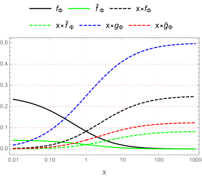
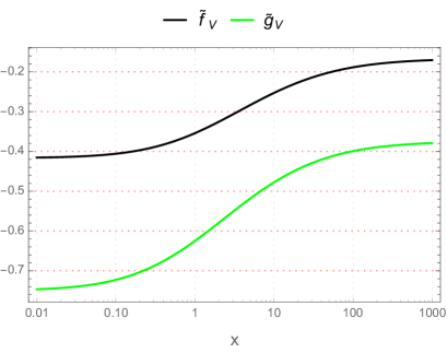
Figure 1: The dependence of master formulas as functions of $x=m_{E}^{2}/m_{X}^{2}$ and $m^{2}_{n_{i}}/m_{X}^{2}$ with $X=W,Y,H^{\pm}_{1,2},H^{A}$.

To estimate the one-loop contributions to AMM, it is useful to see the limits for the above master functions as follows:

$$\lim_{x\to 0}f_{\Phi}(x)=f_{\Phi}(0)=\frac{1}{4},\quad\lim_{x\to\infty}f_{\Phi}(x)=f_{\Phi}(\infty)=0,$$

$$\lim_{x\to 0}\tilde{f}_{\Phi}(x)=\tilde{f}_{\Phi}(0)=\frac{1}{24},\quad\lim_{x\to\infty}\tilde{f}_{\Phi}(x)=\tilde{f}_{\Phi}(\infty)=0,$$

$$\lim_{x\to 0}\tilde{f}_{V}(x)=\tilde{f}_{V}(0)=-\frac{5}{12},\quad\lim_{x\to\infty}\tilde{f}_{V}(x)=\tilde{f}_{V}(\infty)=-\frac{1}{6},$$

$$\lim_{x\to 0}\tilde{g}_{V}(x)=\tilde{g}_{V}(0)=-\frac{3}{4},\quad\lim_{x\to\infty}\tilde{g}_{V}(x)=\tilde{g}_{V}(\infty)=-\frac{3}{8},$$

$$\lim_{x\to 0}\left[x\times f_{\Phi}(x)\right]=0,\quad\quad\lim_{x\to\infty}\left[x\times f_{\Phi}(x)\right]=\frac{1}{4},$$

$$\lim_{x\to 0}\left[x\times\tilde{f}_{\Phi}(x)\right]=0,\quad\quad\lim_{x\to\infty}\left[x\times\tilde{f}_{\Phi}(x)\right]=\frac{1}{12},$$

$$\lim_{x\to 0}\left[x\times g_{\Phi}(x)\right]=0,\quad\quad\lim_{x\to\infty}\left[x\times g_{\Phi}(x)\right]=\frac{1}{2},$$

$$\lim_{x\to 0}\left[x\times\tilde{g}_{\Phi}(x)\right]=0,\quad\quad\lim_{x\to\infty}\left[x\times\tilde{g}_{\Phi}(x)\right]=\frac{1}{8}.$$ (97)

Because $|\beta|\leq\sqrt{3}$, we have $-1\leq B\leq 2$. It is easily to show that:

$$\left|xf_{\Phi}\left(x\right)+Bxg_{\Phi}\left(x\right)\right|\leq\mathcal{O}(1),\;\left|x\tilde{f}_{\Phi}\left(x\right)+Bx\tilde{g}_{\Phi}\left(x\right)\right|\leq\mathcal{O}(1),\;\left|\tilde{f}_{V}\left(x\right)+B\tilde{g}_{V}\left(x\right)\right|\leq\frac{7}{6},$$

$$0\leq\tilde{f}_{V}\left(x\right)+\frac{5}{12}\leq\frac{5}{12},\;0\leq xf_{\Phi}\left(x\right)\leq\frac{1}{4}.$$ (98)

First, we consider the one-loop contribution from the SM gauge $W^{\pm}$ where the deviation from the SM prediction derived from Eq. (94) satisfies:

$$\left|\Delta a_{\mu}(W)\right|\simeq 9.19\times 10^{-9}\left|\left(R^{*}R^{T}\right)_{aa}\times\left(\tilde{f}_{V}\left(x_{W}\right)+\frac{5}{12}\right)\right|<2.5\times 10^{-11}<a^{\mathrm{NP}}_{\mu},$$ (99)

where the constraint $|\left(R^{*}R^{T}\right)_{aa}|\leq 2\times 10^{-3}$ consistent with non-unitary condition (75). In Eq. (99), $\Delta a_{\mu}$ is considered as the $1\sigma$ range of the discrepancy between the SM’s prediction and experiments shown in Eq. (1), namely $\left|\Delta a_{\mu}(W)\right|\ll\Delta a_{\mu}\in\left[1.92\times 10^{-9},\;3.1\times 10^{-9}\right]$. Therefore, we will use the following approximation for both frameworks MSS and ISS:

$$\Delta a_{\mu}(W)\simeq 0.$$ (100)

For the recent bound of the $SU(3)_{L}$ scale, we can use the lower bound $m_{Y}\geq 1$ TeV, consistent with the recent constraint concerned for 3-3-1 models Coutinho:2013lta ; Salazar:2015gxa ; Long:2018fud ; Nepomuceno:2019eaz . Now the one-loop contributions from $H^{A}$ and $Y^{A}$ can be estimated as follows:

$$0<-a_{\mu}(H^{A})\leq 9.19\times 10^{-9}\times\left[\frac{m_{W}^{2}}{m^{2}_{Y}}+\frac{m^{2}_{\mu}}{m^{2}_{E}c^{2}_{\beta}}+\frac{m_{W}^{4}c^{2}_{\beta}}{m_{Y}^{4}}\right]<6.3\times 10^{-11}\ll\Delta a^{\mathrm{NP}}_{\mu},$$

$$0<\Delta a_{\mu}(Y)\leq 9.19\times 10^{-9}\times\frac{m_{W}^{2}}{m^{2}_{Y}}\times\frac{7}{6}<7\times 10^{-11}\ll\Delta a^{\mathrm{NP}}_{\mu}.$$ (101)

where a crude lower bound $m_{E}c_{\beta}\geq 5$ GeV was used. We conclude that the two one-loop contributions originated from heavy Higgs $H^{A}$ and charged gauge boson $Y$ is much smaller than $\Delta a^{\mathrm{NP}}_{\mu}\sim\mathcal{O}(10^{-9})$, which is considered as the $1\sigma$ range given in Eq. (1) from now on. This agrees with all previous works, for example for the heavy charged gauge bosons Pinheiro:2021mps . We will ignore them from now on.

We now discuss on the dominant contributions of the two singly charged Higgs bosons given in Eq. (IV), where small $t_{\beta}$ supports large values of these contributions. The reasonable values for a numerical estimation are $t^{-1}_{\beta}s_{\alpha}c_{\alpha}\simeq 0.5$, and $v/(\sqrt{2}m_{\mu})=1.6\times 10^{3}$, max$[|x_{1}f_{\Phi}\left(x_{1}\right)-x_{2}f_{\Phi}\left(x_{2}\right)|]\simeq 0.25$, we have

$$\left|\sum_{k=1}^{2}\Delta a_{\mu}(H^{\pm}_{1})\right| \leq 1.9\times 10^{-9}\left[10^{3}\left(M_{0}^{-1}M_{D}^{\dagger}Y^{h}\right)_{22}\right]\sim\Delta a^{\mathrm{NP}}_{\mu}\left[10^{3}\left(M_{0}^{-1}M_{D}^{\dagger}Y^{h}\right)_{22}\right].$$ (102)

In the next discussion for two specific frameworks of MSS and ISS, the allowed values of $\left|\left(M_{0}^{-1}M_{D}^{\dagger}Y^{h}\right)_{22}\right|$ will depend strictly on the characteristics of the two models. We will show that the condition (102) will satisfy for only the ISS mechanism, which allows this value to reach the $(g-2)_{\mu}$ data. For convenience, we will use the following estimation,

$$\frac{v}{\sqrt{2}m_{\mu}} \simeq 1.6\times 10^{3};\;|x_{1}f_{\Phi}\left(x_{1}\right)-x_{2}f_{\Phi}\left(x_{2}\right)|\leq 0.25;\;0.3\leq t_{\beta}\leq 10;$$

$$\left|s_{\alpha}c_{\alpha}\right| =\left|\frac{\sin(2\alpha)}{2}\right|\leq 0.5;\;m_{H^{\pm}_{1}},\;m_{H^{\pm}_{2}}\geq 800\;\mathrm{GeV};M_{0}\geq 100\;\mathrm{GeV}.$$ (103)

After that, other possible values of $m_{H^{\pm}_{K}}$, $M_{0}$, and $t_{\beta}$ will also be discussed.

Now we will derive the specific analytic formulas of one-loop contributions to $\Delta a_{\mu}$ corresponding to the two mechanisms MSS and ISS. We note that all above discussions for $\Delta a_{\mu}$ are applied in the same way to derive to $\Delta a_{e}$, therefore, we just mention to $\Delta a_{\mu}$ in the numerical discussion.

IV.1 The MSS mechanism

The MSS relations given in Eqs. (57) and (58) result in that

$$M_{D}^{\dagger}R^{\dagger}=\hat{m}_{\nu},\;R=-iU_{\mathrm{PMNS}}\left(\frac{\hat{m}_{\nu}}{M_{0}}\right)^{1/2},\;\quad m_{n_{4,5,6}}\simeq M_{0}.$$ (104)

The detailed derivation of the one-loop contributions from singly charged Higgs bosons is given in appendix B. Using $\tilde{f}_{\Phi}(0)=\frac{1}{24}$, the one-loop contribution from $H^{\pm}_{1}$ is

$$\Delta a^{\mathrm{MSS}}_{\mu}(H^{\pm}_{1}) =-9.19\times 10^{-9}$$

$$\times\mathrm{Re}\left\{\left[c^{2}_{\alpha}\left(\frac{m^{2}_{n_{2}}}{M_{0}^{2}}\right)^{1/2}+\frac{vt_{\beta}^{-1}c_{\alpha}s_{\alpha}}{\sqrt{2}m_{\mu}}\sum_{c=1}^{3}\left(\frac{m^{2}_{n_{c}}}{M_{0}^{2}}\right)^{1/4}U_{\mathrm{PMNS},2c}\left(-iY^{h}\right)_{c2}\right]x_{1}f_{\Phi}(x_{1})\right.$$

$$\quad+t_{\beta}^{-2}c^{2}_{\alpha}\sum_{c=1}^{3}\left|U_{\mathrm{PMNS},2c}\right|^{2}\left[\frac{m_{n_{c}}^{2}}{m^{2}_{H^{\pm}_{1}}}\left(\frac{1}{24}-\tilde{f}_{\Phi}(x_{1})\right)+\frac{m_{n_{c}}}{M_{0}}x_{1}\tilde{f}_{\Phi}(x_{1})\right]$$

$$\quad+\frac{m^{2}_{\mu}t_{\beta}^{2}c_{\alpha}^{2}}{m^{2}_{H^{\pm}_{1}}}\left[\frac{1}{24}-\sum_{c=1}^{3}\left|U_{\mathrm{PMNS},2c}\right|^{2}\frac{m_{n_{c}}}{M_{0}}\left(\frac{1}{24}-\tilde{f}_{\Phi}(x_{1})\right)\right]$$

$$\quad+\frac{v^{2}s_{\alpha}^{2}}{2m^{2}_{H^{\pm}_{1}}}\left[\sum_{c=1}^{3}\left|Y^{h}_{c2}\right|^{2}\frac{m_{n_{c}}}{M_{0}}\left(\frac{1}{24}-\tilde{f}_{\Phi}(x_{1})\right)+\left(Y^{h\dagger}Y^{h}\right)_{22}\tilde{f}_{\Phi}(x_{1})\right]$$

$$\quad-\left.\frac{vm_{\mu}t_{\beta}s_{2\alpha}}{\sqrt{2}m^{2}_{H^{\pm}_{1}}}\left[\left(-iU_{\mathrm{PMNS}}\left(\frac{\hat{m}^{2}_{\nu}}{M^{2}_{0}}\right)^{1/4}Y^{h}\right)_{22}\left(\frac{1}{24}-\tilde{f}_{\Phi}(x_{1})\right)\right]\right\}.$$ (105)

It can be seen that only two terms proportional to $\left(\frac{m^{2}_{n_{c}}}{M^{2}_{0}}\right)^{1/4}\mathrm{Re}[(-iU_{\mathrm{PMNS},2c}Y^{h}_{c2})]$ can give contributions having consistent sign with $\Delta a^{\mathrm{NP}}_{\mu}$, and $\mathrm{Re}[(-iU_{\mathrm{PMNS},2c}Y^{h}_{c2})]$ must be negative (see the first and last lines in the real part of Eq. (IV.1)). We just focus on these two contributions. The remaining terms always give negative contributions to $\Delta a^{\mathrm{NP}}_{\mu}$. The two mentioned terms can be estimated as follows:

$$0<\left(\frac{m^{2}_{n_{c}}}{M_{0}^{2}}\right)^{1/4}\times x_{1}f_{\Phi}(x_{1})\leq\left(\frac{(0.12\;\mathrm{eV})^{2}}{m_{H^{\pm}_{1}}^{2}}\right)^{1/4}\times x_{1}^{3/4}f_{\Phi}(x_{1})<1.1\times 10^{-7},$$

$$0<\left(\frac{m^{2}_{n_{c}}}{M_{0}^{2}}\right)^{1/4}\times\left(\frac{1}{24}-\tilde{f}_{\Phi}(x_{1})\right)\leq\frac{1}{24}\left(\frac{(0.12\;\mathrm{eV})^{2}}{m_{H^{\pm}_{1}}^{2}}\right)^{1/4}<10^{-7},$$ (106)

where we have used $m_{H^{\pm}_{1}}\geq 100$ GeV and max$[x_{1}^{3/4}f_{\Phi}(x_{1})]<0.1$. But in this situation the factor $\left|\frac{v}{\sqrt{2}m_{\mu}}Y^{h}_{c2}t^{-1}_{\beta}\right|\leq 10^{4}$ is still not large enough so that the total can give any significant contributions to $\Delta a^{\mathrm{MSS}}_{\mu}$. In conclusion, the MSS mechanism still fails to explain the experimental AMM data of $\mu$.

IV.2 The ISS mechanism

The ISS mechanism will be considered instead of the MSS one. The change is for only singly charged Higgs bosons $H^{\pm}_{k}$. Following Eqs. (63) and (III), the results for $H^{\pm}_{1,2}$ are

$$a^{\mathrm{ISS}}_{\mu}(H^{\pm}_{1}) =-9.19\times 10^{-9}$$

$$\times\mathrm{Re}\left\{\sum_{c=1}^{3}\left[c^{2}_{\alpha}\left|U_{\mathrm{PMNS},2c}\right|^{2}\frac{m_{n_{c}}}{\mu_{X}}+\frac{vt_{\beta}^{-1}c_{\alpha}s_{\alpha}}{\sqrt{2}m_{\mu}}U_{\mathrm{PMNS},2c}\left(\frac{m_{n_{c}}}{\mu_{X}}\right)^{1/2}\left(Y^{h}_{2}\right)_{c2}\right]x_{1}f_{\Phi}(x_{1})\right.$$

$$\quad+\sum_{c=1}^{3}\left[\left|U_{\mathrm{PMNS},2c}\right|^{2}\left(t_{\beta}^{-2}c^{2}_{\alpha}\frac{m_{n_{c}}}{\mu_{X}}\right)\right]x_{1}\tilde{f}_{\Phi}(x_{1})$$

$$\quad+\frac{m^{2}_{\mu}t_{\beta}^{2}c_{\alpha}^{2}}{m^{2}_{H^{\pm}_{1}}}\left[\frac{1}{24}-\sum_{c=1}^{3}\left[\left|U_{\mathrm{PMNS},2c}\right|^{2}\frac{m_{n_{c}}}{\mu_{X}}\right]\left(\frac{1}{24}-\tilde{f}_{\Phi}(x_{1})\right)\right]$$

$$\quad+\frac{v^{2}s_{\alpha}^{2}}{2m^{2}_{H^{\pm}_{1}}}\left[\sum_{c=1}^{3}\left[\left|\left(Y^{h}_{2}\right)_{c2}\right|^{2}\frac{m_{n_{c}}}{\mu_{X}}\right]\left(\frac{1}{24}-\tilde{f}_{\Phi}(x_{1})\right)+\left(Y^{h\dagger}_{2}Y^{h}_{2}\right)_{22}\tilde{f}_{\Phi}(x_{1})\right]$$

$$\quad-\left.\frac{vm_{\mu}t_{\beta}s_{2\alpha}}{\sqrt{2}m^{2}_{H^{\pm}_{1}}}\left(\frac{1}{24}-\tilde{f}_{\Phi}(x_{1})\right)\sum_{c=1}^{3}\left[U_{\mathrm{PMNS},2c}\left(Y^{h}_{2}\right)_{c2}\left(\frac{m_{n_{c}}}{\mu_{X}}\right)^{1/2}\right]\right\},$$

$$a^{\mathrm{ISS}}_{\mu}(H^{\pm}_{2}) =a_{\mu}(H^{\pm}_{1})\left[x_{1}\to\;x_{2},\;s_{\alpha}\to-c_{\alpha},\;c_{\alpha}\to s_{\alpha}\right],$$ (107)

where we have used the form $Y^{h}=(O_{3\times 3},\;Y^{h}_{2})^{T}$ for the ISS framework. Here, the parameter $\mu_{X}$ appears in the ISS mechanism instead of $M_{0}$ corresponding to the MSS. The second term in the first line of Eq. (IV.2) is from $H^{\pm}_{1}$ emphasized previously in Eq. (IV).

Using the constraint (75) for $RR^{\dagger}=U_{\mathrm{PMNS}}\hat{x}_{\nu}U_{\mathrm{PMNS}}^{\dagger}$ we have $\hat{x}_{\nu}<\mathcal{O}(10^{-3})$. Therefore, we will choose a safe upper bound for the NO scheme as follows

$$\mathrm{Max}[\left(\hat{x}_{\nu}\right)_{aa}]=\frac{m_{n_{3}}}{\mu_{X}}\simeq\left(\frac{\Delta m^{2}_{32}}{\mu_{X}^{2}}\right)^{1/2}\leq 2\times 10^{-3}\Rightarrow\mu_{X}\geq 2.5\times 10^{-8}\;\mathrm{GeV}.$$ (108)

The default value of $\mu_{X}$ is fixed by $\mu_{X}=2.5\times 10^{-8}\;\mathrm{GeV}$.

With the allowed range given in Eq. (IV), it can be proved that:

$$0<\sum_{c=1}^{3}c^{2}_{\alpha}\left|U_{\mathrm{PMNS},2c}\right|^{2}\frac{m_{n_{c}}}{\mu_{X}}x_{1}f_{\Phi}(x_{1})<\left|U_{\mathrm{PMNS},23}\right|^{2}\times 5\times 10^{-3}\times\frac{1}{12}\simeq 8.9\times 10^{-5},$$

$$0<a^{\mathrm{ISS}}_{\mu,1}(H_{1}^{\pm})\sim\sum_{c=1}^{3}\left[\left|U_{\mathrm{PMNS},2c}\right|^{2}\left(t_{\beta}^{-2}c^{2}_{\alpha}\frac{m_{n_{c}}}{\mu_{X}}\right)\right]x_{1}\tilde{f}_{\Phi}(x_{1})<1.3\times 10^{-3},$$

$$0<\frac{m^{2}_{\mu}t_{\beta}^{2}c_{\alpha}^{2}}{m^{2}_{H^{\pm}_{1}}}\left[\frac{1}{24}-\sum_{c=1}^{3}\left[\left|U_{\mathrm{PMNS},2c}\right|^{2}\frac{m_{n_{c}}}{\mu_{X}}\right]\left(\frac{1}{24}-\tilde{f}_{\Phi}(x_{1})\right)\right]<10^{-7}$$

$$0<\frac{v^{2}s_{\alpha}^{2}}{2m^{2}_{H^{\pm}_{1}}}\times\sum_{c=1}^{3}\left[\left|Y^{h}_{(c+3)2}\right|^{2}\frac{m_{n_{c}}}{\mu_{X}}\right]\left(\frac{1}{24}-\tilde{f}_{\Phi}(x_{1})\right)<0.32\times 10^{-4},$$

$$0<\frac{vm_{\mu}t_{\beta}s_{2\alpha}}{\sqrt{2}m^{2}_{H^{\pm}_{1}}}\left(\frac{1}{24}-\tilde{f}_{\Phi}(x_{1})\right)\sum_{c=1}^{3}\left[\mathrm{Re}[U_{\mathrm{PMNS},2c}Y^{h}_{(c+3)2}]\left(\frac{m_{n_{c}}}{\mu_{X}}\right)^{1/2}\right]<10^{-6},$$

$$0<a^{\mathrm{ISS}}_{\mu,2}(H_{1}^{\pm})\sim\frac{v^{2}s_{\alpha}^{2}}{2m^{2}_{H^{\pm}_{1}}}\left(Y^{h\dagger}Y^{h}\right)_{22}\tilde{f}_{\Phi}(x_{1})=\frac{v^{2}s_{\alpha}^{2}}{2m^{2}_{H^{\pm}_{1}}}\left(Y^{h\dagger}_{2}Y^{h}_{2}\right)_{22}\tilde{f}_{\Phi}(x_{1})<1.6\times 10^{-2}.$$ (109)

There are only two contributions $a_{\mu,1(2)}(H_{1}^{\pm})$ in the second and last lines that may affect significantly $a_{\mu}(H^{\pm}_{1})$ because of the rather large upper bounds $a_{\mu,1}(H_{1}^{\pm})\leq 1.3c^{2}_{\alpha}\times 10^{-11}$ and $a_{\mu,2}(H_{1}^{\pm})\leq 23s^{2}_{\alpha}\times 10^{-11}$. But both of them give negative contributions to $\Delta a^{\mathrm{ISS}}_{\mu}$, hence should be small. Ignoring all other contributions smaller $10^{-4}\times\Delta a^{\mathrm{NP}}_{\mu}$, the remaining large contribution in Eq. (IV.2) is the one mentioned in Eq. (IV). It has the following form in the ISS framework:

$$a^{\mathrm{ISS}}_{\mu,0}(H^{\pm}) =-9.19\times 10^{-9}\mathrm{Re}\left\{\frac{vt_{\beta}^{-1}c_{\alpha}s_{\alpha}}{\sqrt{2}m_{\mu}}\left(\frac{m_{n_{3}}}{\mu_{X}}\right)^{1/2}Y^{d}_{2}\left[x_{1}f_{\Phi}(x_{1})-x_{2}f_{\Phi}(x_{2})\right]\right\}$$

$$=-680.58\times 10^{-9}\times t_{\beta}^{-1}c_{\alpha}s_{\alpha}\left(\frac{m_{n_{3}}}{\mu_{X}}\right)^{1/2}Y^{d}_{2}\left[x_{1}f_{\Phi}(x_{1})-x_{2}f_{\Phi}(x_{2})\right],$$ (110)

where the part relating to $x_{k}$ is the contribution from $H^{\pm}_{k}$ exchange, and the new parameter $Y^{d}_{2}$ is assumed to relate to Yukawa coupling matrix $Y^{h}_{2}$ through the following relation

$$U_{\mathrm{PMNS}}\left(\frac{\hat{m}_{\nu}}{m_{n_{3}}}\right)^{1/2}Y^{h}_{2}\equiv\mathrm{diag}\left(Y^{d}_{1},\;Y^{d}_{2},Y^{d}_{3}\right)=Y^{d},$$ (111)

so that the two largest one-loop contributions from $H^{\pm}_{1,2}$ to AMM will allow zero contributions to the cLFV branching ratios Br$(e_{b}\to e_{a}\gamma)\sim\left(|c_{(ab)R}|^{2}+|c_{(ba)R}|^{2}\right)$ Crivellin:2018qmi , because $c_{(ab)R}(H^{\pm}),c_{(ba)R}(H^{\pm})\sim\left(U_{\mathrm{PMNS}}\hat{m}_{\nu}^{1/2}Y^{h}_{2}\right)_{ab,ba}(H^{\pm})=0$ for $a\neq b$. Now, the matrix $Y^{h}_{2}$ is derived through the following relation:

$$Y^{h}_{2}=\left(\frac{\hat{m}_{\nu}}{m_{n_{3}}}\right)^{-1/2}U^{\dagger}_{\mathrm{PMNS}}Y^{d},$$ (112)

which will be used to check the perturbative limit of all $\left|(Y^{h}_{2})_{ab}\right|<\sqrt{4\pi}\simeq 3.5$ while scanning values of $Y^{d}_{1,2,3}$. In this case, the factors $\left(\frac{(\hat{m}_{\nu})_{aa}}{m_{n_{3}}}\right)^{-1/2}\geq 1$ in the NO scheme and all active neutrino masses lie in the denominators. Therefore, these masses must be non-zero and large enough to guarantee that all entries of $Y^{h}_{2}$ satisfy the perturbative limits.

From now on, we will fix $m_{n_{1}}=0.01$ eV in our numerical discussion. Smaller $m_{n_{1}}$ will give smaller allowed $Y^{d}_{1}$ satisfying the perturbative limit of $Y^{h}_{2}$. Using the best-fit points corresponding to the NO scheme of neutrino oscillation data given in Eq. (III), $Y^{h}_{2}$ has the following form

$$Y^{h}_{2}=\left(\begin{array}[]{ccc}1.84Y^{d}_{1}&(-0.7-0.125i)Y^{d}_{2}&(1.09-0.113i)Y^{d}_{3}\\ 1.1Y^{d}_{1}&(1.184-0.074i)Y^{d}_{2}&(-1.11-0.068i)Y^{d}_{3}\\ (-0.116-0.09i)Y^{d}_{1}&0.732Y^{d}_{2}&0.666Y^{d}_{3}\\ \end{array}\right).$$ (116)

For small $m_{n_{1}}$ including the case $m_{n_{1}}=0$, matrix $Y^{h}_{2}$ is chosen as follows:

$$Y^{h}_{2}=\left(\begin{array}[]{ccc}0&0&0\\ (2.9+0.3i)Y^{d}_{1}&(0.50-0.32i)Y^{d}_{2}&(0.61-0.68i)Y^{d}_{3}\\ (-1.23-0.21i)Y^{d}_{1}&(1.15+0.12i)Y^{d}_{2}&Y^{d}_{3}\\ \end{array}\right),$$ (120)

which $Y^{d}$ defined from Eq. (65) is not diagonal, but it always keeps $(Y^{d})_{12}=(Y^{d})_{21}=(Y^{d})_{13}=0$. In addition, $Y^{d}_{3}=0$ gives $(Y^{d})_{32}=0$. This will avoid large contributions to the strict constraint of cLFV decay Br$(\mu\to e\gamma)$. The numreical investigations show that the two choices of $Y^{h}_{2}$ mentioned above have the same qualitative results. Numerical illustration will be done with the $Y^{h}_{2}$ given in Eq. (116). Therefore, we will fix $Y^{d}_{3}=0$ in our numerical investigation on $a^{\mathrm{ISS}}_{e,\mu}(H^{\pm})$. We note that $Y^{d}_{3}$ also contributes to the AMM of the $\tau$ lepton, which still has weak constraints from recent experiments OPAL:1998dsa ; L3:1998lhr ; DELPHI:2003nah and a combination derived from these experimental results Gonzalez-Sprinberg:2000lzf ; Eidelman:2016aih , see discussions on this topic in Refs. Tran:2020tsj ; Crivellin:2021spu , suggesting new experiments to improve measurements.

Similarly, the data of $\Delta a^{\mathrm{NP}}_{e}$ may be explained by the following contribution:

$$a^{\mathrm{ISS}}_{e,0}(H^{\pm}) =-9.19\times 10^{-9}\times\frac{m_{e}^{2}}{m^{2}_{\mu}}\mathrm{Re}\left\{\frac{vt_{\beta}^{-1}c_{\alpha}s_{\alpha}}{\sqrt{2}m_{e}}\left(\frac{m_{n_{3}}}{\mu_{X}}\right)^{1/2}Y^{d}_{1}\left[x_{1}f_{\Phi}(x_{1})-x_{2}f_{\Phi}(x_{2})\right]\right\}$$

$$=-32409\times 10^{-13}\times t_{\beta}^{-1}c_{\alpha}s_{\alpha}\left(\frac{m_{n_{3}}}{\mu_{X}}\right)^{1/2}Y^{d}_{1}\left[x_{1}f_{\Phi}(x_{1})-x_{2}f_{\Phi}(x_{2})\right].$$ (121)

In the simple forms of the matrices $Y^{h}$ given in Eq. (112) and $M_{D}$ we assumed here, the main difference between $a^{\mathrm{ISS}}_{e,0}(H^{\pm})$ and $a^{\mathrm{ISS}}_{\mu,0}(H^{\pm})$ is that they contain different free factors $Y^{d}_{1}$ and $Y^{d}_{2}$, respectively. The numerical results show that this difference is enough to explain both AMM data of $e$ and $\mu$ at $1\sigma$ discrepancy given in Eqs. (1) and (2). The regions of the parameter space satisfying simultaneously these will be defined as the allowed regions from now on.

The first numerical illustrations are shown in Fig. 2, where free parameters are fixed in the ranges given in (IV) and predict valid regions satisfying both the experimental AMM data of muon (two upper panels) and electron (two lower panels).

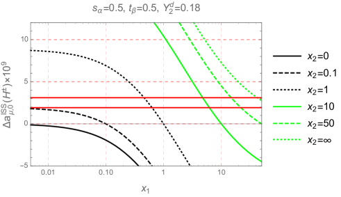
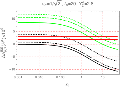
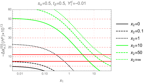
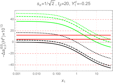
Figure 2: The dependence of $\Delta a^{\mathrm{ISS}}_{\mu,0}(H^{\pm})$ and $\left[-\Delta a^{\mathrm{ISS}}_{e,0}(H^{\pm})\right]$ as functions of $x_{1}$ with different fixed $x_{2}$. The red lines show the $1\sigma$ allowed ranges of $\Delta a^{\mathrm{NP}}_{\mu}$ and $\Delta a^{\mathrm{NP}}_{e}$ given in Eqs. (1) and (2), respectively.

In addition, in the upper left panel of Fig. 2, the numerical values $s_{\alpha}=0.5$, $Y^{d}_{2}=0.21$, and $t_{\beta}=0.5$ safely satisfy perturbative limits of max$|\left(Y^{h}_{2}\right)_{ab}|<0.2$. On the other hand, numerical values of free parameters in the upper right panel are somewhat special: $s_{\alpha}=1/\sqrt{2}$ is maximal for $s_{2\alpha}=1$, large $Y^{d}_{2}=2.8$ close the perturbative limit max$|\left(Y^{h}_{2}\right)_{ab}|=3.32$, and $t_{\beta}=20\gg 1$ does not support large $a^{\mathrm{ISS}}_{\mu}(H^{\pm})$, which excludes the regions satisfying $0<x_{2}<0.1$ and all $x_{1}>0$, for example. All values of $t_{\beta}>30$ are excluded in this case. We conclude that the AMM data will result in a upper bound of $t_{\beta}$. The values of $Y^{d}_{1}$ are chosen so that there exist allowed values of $(x_{1},x_{2})$ satisfying simultaneously both $1\sigma$ experimental AMM data of muon and electron. Namely, the allowed values of $(x_{1},\;x_{2})$ in the two left panels are in the ranges $0<x_{1}\leq 20$ and $0.1<x_{2}$. Similarly, the allowed regions in the two right panels satisfy $0<x_{1}\leq 10$ and $x_{2}>0.1$. Large $t_{\beta}$ gives strong upper constraint on $M_{0}<750$ GeV derived from the perturbative limit of max$|Y^{X}_{ab}|$=max$\frac{\sqrt{2}\left(m_{D}\right)_{ab}}{v_{2}}=$ max$\frac{M_{0}\sqrt{2}\left(\hat{x}_{\nu}^{1/2}U^{\dagger}_{\mathrm{PMNS}}\right)_{ab}}{vc_{\beta}}<3.5$. Consequently, $x_{k}=M_{0}^{2}/m^{2}_{H_{k}}$ should not be too large so that $m_{H_{k}}$ are larger than the lower bounds from experiments.

In general, the allowed regions of parameter space depend strongly on the $\hat{x}_{\nu}$, namely larger $\hat{x}_{\nu}$ will allow larger $t_{\beta}$, and smaller values of other parameters including $s_{2\alpha}\equiv 2s_{\alpha}c_{\alpha}$, $Y^{d}_{1}$, and $Y^{d}_{2}$. Defining that $\hat{x}_{\nu}=\left(\hat{m}_{\nu}/m_{n_{3}}\right)\times\hat{x}_{\nu 3}$ with $\hat{x}_{\nu 3}=\frac{m_{n_{3}}}{\mu_{X}}$ and fixed $m_{n_{1}}=0.01$ eV, $a^{\mathrm{ISS}}_{e,\mu}(H^{\pm})$ given in Eq. (IV.2) depends strongly on $\hat{x}_{\nu 3}$. With large $\hat{x}_{\nu 3}\in\left[10^{-3},\;5\times 10^{-3}\right]$ the allowed ranges of free parameters are given in Table 1.

	$t_{\beta}$	$s_{\alpha}\left\{-,\;+\right\}$	$M_{0}$ [TeV]	$m_{H_{1}^{\pm}}$ [TeV]	$m_{H_{2}^{\pm}}$ [TeV]	$Y_{1}^{d}\left\{-,\;+\right\}$	$Y_{2}^{d}\left\{-,\;+\right\}$
Min	$\;0.320$	$\{-0.987,\;0.004\}$	0.194	0.806	0.801	$\{-0.364,\;0.019\}$	$\{-2.95,\;0.311\}$
Max	$\;22.932$	$\{-0.039,\;0.998\}$	4.998	49.67	49.03	$\{-0.018,\;0.376\}$	$\{-0.388,\;2.95\}$

Table 1: Allowed ranges of free parameters with large $\;10^{-3}\leq\hat{x}_{\nu 3}=\frac{m_{n_{3}}}{\mu_{X}}\leq 5\times 10^{-3}$, the notations $-$ ($+$) denote the negative (positive) ranges of the allowed regions.

We note that $s_{\alpha}$ never vanishes, namely large $\hat{x}_{\nu 3}\leq 5\times 10^{-3}$ can allow rather small $|s_{\alpha}|\geq 10^{-3}$, provided that $t_{\beta}\to 0.3$. This property distinguishes completely to the conclusion given in Ref. Hue:2021xap , where the allowed regions with fixed $s_{\alpha}=0$ require a necessary condition of large $t_{\beta}>30$.

In this last discussion we will focus on the allowed regions consisting of light masses of heavy neutrinos and singly charged Higgs bosons. Namely in the ISS realization, heavy neutrinos can be detected by future searches at colliders such as Large Hadron Collider (LHC) and the International Linear Collider (ILC), and Large Hadron electron Collider (LHeC) LHeCStudyGroup:2012zhm , where the heavy neutrinos mass range from $\mathcal{O}(10^{2})$ GeV to few TeV were discussed Das:2012ze ; Das:2014jxa ; Das:2015toa ; Das:2016hof ; Das:2018usr . Namely, because of the not too small mixing $\sim\sqrt{x_{\nu,3}}$ between ISS and active neutrinos $\nu_{aL}$, the main production channel of heavy neutrinos $n_{I}$ (I=4,…,9) with mass $M_{0}$ at LHC is $u\bar{d}\to n_{I}e^{+}_{a}$ through the $s$ channel exchanging $W$ boson. Then the decay channel of $n_{I}$ may be $n_{I}\to e_{a}^{-}W^{+},n_{a}Z,\;n_{a}h$, where $h$ is the standard model-like Higgs boson. The ILC can produce heavy neutrino in the processes $e^{+}e^{-}\to\bar{n}_{a}n_{I}$ through $t$ and $s$-channels exchanging the $W$ and $Z$ bosons, respectively. The model under consideration also predicts a channel producing two heavy neutrinos $e^{+}e^{-}\to\bar{n}_{I}n_{I}$ through exchanging $H^{\pm}_{k}$. In the following numerical discussion, the allowed regions are defined as they result in the two values of $\Delta a^{\mathrm{ISS}}_{\mu}$ and $\Delta a^{\mathrm{ISS}}_{e}$ satisfying both AMM experimental data of $\mu$ and electron at 1 $\sigma$ discrepancy level, and all Yukawa couplings satisfy perturbative limits, $|(Y^{h}_{2})_{ab}|,|Y^{X}_{ab}|\leq\sqrt{4\pi}$ with $a,b\leq 3$. The region of parameter space used to scan is chosen as follows:

$$\;m_{H^{\pm}_{1}},\;m_{H^{\pm}_{2}}\geq 800\;\mathrm{GeV};10\;\mathrm{GeV}\leq M_{0}\leq\;5\times 10^{3}\;\mathrm{GeV};\;0.01\leq x_{1},x_{2}\leq 100,$$

$$0.3\leq t_{\beta}\leq 50;\;\left|s_{\alpha}\right|\leq 1.;\;|Y^{d}_{1}|,\;|Y^{d}_{2}|\leq 4.5;\;10^{-7}\leq\;\hat{x}_{\nu 3}=\frac{m_{n_{3}}}{\mu_{X}}\leq 10^{-3}.$$ (122)

The scanning range of $\hat{x}_{\nu 3}$ satisfies the non-unitary constraint given in Eq. (75). The numerical results confirm that $\left|a^{\mathrm{ISS}}_{\mu,1}(H^{\pm})/a^{\mathrm{ISS}}_{\mu}(H^{\pm})\right|<4\%$, and $\left|a^{\mathrm{ISS}}_{\mu,2}(H^{\pm})/a^{\mathrm{ISS}}_{\mu}(H^{\pm})\right|<10^{-5}$. Therefore, these suppressed values are not shown in detail. The allowed regions are more strict than the scanned region given in (IV.2), see Table 2.

	$t_{\beta}$	$s_{\alpha}$	$\hat{x}_{\nu 3}$	$M_{0}$ [TeV]	$m_{H_{1}^{\pm}}$ [TeV]	$m_{H_{2}^{\pm}}$ [TeV]	$Y^{d}_{1}$	$Y^{d}_{2}$
Min	0.3	-0.99	$3.9\times 10^{-7}$	0.318	0.8	0.8	-0.361	-2.95
Max	21.42	0.996	$10^{-3}$	5.	48	48.	0.352	2.949

Table 2: Allowed ranges of free parameters corresponding to the scanning region (IV.2).

In addition, values of $|s_{\alpha}|$, $|Y^{d}_{1}|$, and $|Y^{d}_{2}|$ are bounded from below:

$$s_{\alpha} \in[-0.99,\;-0.029]\cup[0.026,\;0.996]\to s_{2\alpha}\in[-1,\;-0.058]\cup[0.051,\;1],$$

$$\;Y^{d}_{1} \in[-0.361,\;-0.024]\cup[0.015,\;0.352],\;Y^{d}_{2}\in[-2.95,\;-0.176]\cup[0.523,\;2.95],$$ (123)

where we define $s_{2\alpha}=2s_{\alpha}c_{\alpha}$. Here although the lower bound of $t_{\beta}$ is the perturbative limit chosen in the scanned range, the upper bound is more strict than the largest value of the scanned range $t_{\beta}<21.42<50$. In general, the allowed regions require all lower bounds for free parameters $\hat{x}_{\nu 3}\geq 3.9\times 10^{-7}$, $M_{0}\geq 318.$ GeV, $|Y^{d}_{2}|\geq 0.176$, and $|s_{2\alpha}|>0.051$. Values of $Y^{d}_{1}$ are bounded in a more strict range of $0.015<|Y^{d}_{1}|<0.352$. The lower bound of $M_{0}$ supports many promoting channels to search for heavy neutrinos at both LHC and ILC Das:2012ze ; Das:2014jxa ; Das:2015toa ; Das:2016hof .

The correlations between free parameters and $a^{\mathrm{ISS}}_{\mu}(H^{\pm})$ in the allowed regions are illustrated in Fig. 3 with 2000 allowed points collected.

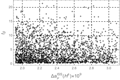
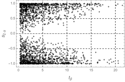
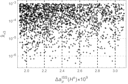
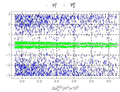
Figure 3: The correlations of free parameters vs. $\Delta a^{\mathrm{ISS}}_{\mu}(H^{\pm})$ and $t_{\beta}$ in the allowed regions.

The correlations of $\Delta a_{e}(H^{\pm})$ vs. $\Delta a_{\mu}(H^{\pm})$ can be seen from the correlations relating with $Y^{d}_{1}$ shown in the lower right panel of Fig. 3. We can see that very large $t_{\beta}$ allows only small $\Delta a_{\mu}(H^{\pm})$. The dependence of $s_{\alpha}$, $Y^{d}_{1}$, and $Y^{d}_{2}$ on $\Delta a_{\mu}(H^{\pm})$ is rather weak. The Fig. 3 shows the consistent approximation we discussed above that $a^{\mathrm{ISS}}_{e_{a}}\simeq a^{\mathrm{ISS}}_{e_{a},0}(H^{\pm})\sim t^{-1}_{\beta}\hat{x}_{\nu_{3}}^{1/2}Y^{d}_{a}s_{2\alpha}$. Namely, the two left panels prefer allowed points with small $t_{\beta}$ and large $\hat{x}_{\nu_{3}}$. While large values of $\Delta a_{\mu}$ near the upper allowed bound exclude large $t_{\beta}$ and too small $\hat{x}_{\nu_{3}}$. In the upper right panel, large $t_{\beta}$ requires large $|s_{2\alpha}|$ so that the ratio $s_{2\alpha}/t_{\beta}$ is large enough to keep $\Delta a_{\mu}$ in the allowed range. In the lower right panel, we cannot realize the linear dependence of $Y^{d}_{2}$ on $\Delta a_{\mu}$ because many values of $Y^{d}_{2}$ are excluded by the pertubative limit of $Y^{h}_{2}$. On the other hand, this property can be seen for $Y^{d}_{1}$ because of the relations $|Y^{d}_{1}|\sim|\Delta a_{\mu,0}/\Delta a_{e,0}|$. In particularly, based on the two dominant contribution of AMM given in Eq. (IV.2) and (IV.2), $\Delta a^{\mathrm{ISS}}_{e_{a},0}\simeq\Delta a^{\mathrm{ISS}}_{e_{a}}$, it is easily to show that $|\Delta a^{\mathrm{ISS}}_{\mu}/\Delta a^{\mathrm{ISS}}_{e}|\simeq$$|\Delta a^{\mathrm{ISS}}_{\mu,0}/\Delta a^{\mathrm{ISS}}_{e,0}|=|m_{\mu}Y^{d}_{2}/(m_{e}Y^{d}_{1})|$. Identifying these with the experimental data will lead to a consequence that $|Y^{d}_{1}|=|m_{\mu}Y^{d}_{2}\Delta a^{\mathrm{NP}}_{e}/(m_{e}\Delta a^{\mathrm{NP}}_{\mu})|\simeq\mathcal{O}(10^{-2})|Y^{d}_{2}|$. Therefore, $|Y_{1}|$ can get small values of $\mathcal{O}(10^{-2})$. Illustrations are shown in Fig. 4,

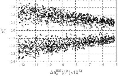
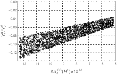
Figure 4: The correlations between $Y^{d}_{1}$ and $Y^{d}_{1}/Y^{d}_{2}$ vs $\Delta a^{\mathrm{ISS}}_{e_{a},0}$.

where the left panel shows that $|Y^{d_{1}}|\sim\Delta a^{\mathrm{ISS}}_{e_{a},0}$ depends nearly linearly on $\Delta a^{\mathrm{ISS}}_{e}$. The right panel shows the valid of the relation $\Delta a^{\mathrm{ISS}}_{e}\simeq a^{\mathrm{ISS}}_{e,0}\sim Y^{d}_{1}/Y^{d}_{2}$ we mentioned above. The band widths appear in the plots originate from the $1\sigma$ ranges of AMM experimental data.

It is also emphasized that $Y^{d}_{1,2}$ may give loop corrections to lepton masses $m_{e,\mu}$ Baker:2020vkh ; Baker:2021yli , where large $|Y^{d}_{1,2}|$ may lead to the fine-tuning problem that loop corrections $\delta m_{\mu,e}\gg m_{\mu,e}$. Our model considered here has the same property with the models in class I with new neutral lepton having $Y_{\psi}=0$. Discussions in Ref. Baker:2021yli suggest that the allowed regions we discussed above may consist of points with small $|Y^{d}_{1,2}|$ enough to avoid this fine-tuning. Determining exactly these regions of the parameter space should be done in the future.

The mass parameters $M_{0}$ and $m_{H^{\pm}_{1,2}}$ are independent with $\Delta a_{\mu}(H^{\pm})$ in the allowed regions. It is more interesting to see the relations between two singly charged Higgs boson masses and $M_{0}$, and between $\hat{x}_{\nu 3}$ and two charged Higgs boson masses and $M_{0}$, see Fig. 5.

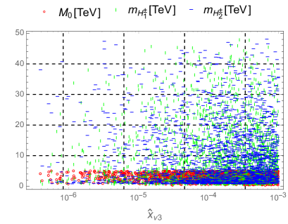
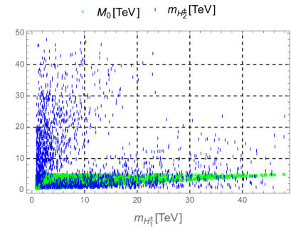
Figure 5: The correlations between different masses vs $\hat{x}_{\nu 3}$ (left panel) and $m_{H^{\pm}_{1}}$ (right panel).

In the left panel, small $\hat{x}_{\nu 3}$ is disfavored and allowed with only large $M_{0}$ up to the upper bound of the scanned range. In the right panel, the allowed region favors both small values of $m_{H^{\pm}_{1}}$ and $m_{H^{\pm}_{2}}$, but requires $|m_{H^{\pm}_{1}}-m_{H^{\pm}_{2}}|\geq 252.4$ GeV.

Other interesting correlations between different free parameters versus $\hat{x}_{\nu 3}$ are shown in Fig. 6.

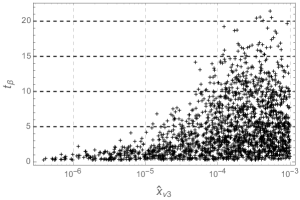
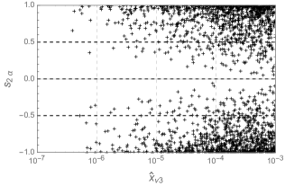
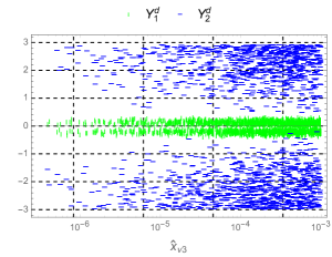
Figure 6: The correlations between different free parameters vs $\hat{x}_{\nu 3}$.

First, the allowed regions favor large $\hat{x}_{\nu 3}$, which supports small $s_{2\alpha}$ and large $t_{\beta}$. In addition, careful numerical investigations show that the recent constraint on $\hat{x}_{\nu 3}$ given in Eq. (75) does not allow $s_{\alpha}=0$ or $t_{\beta}>30$. This conclusion excludes completely the allowed regions indicated in Ref. Hue:2021xap , where large $t_{\beta}>30$ is one of the necessary requirements to explain the experimental $(g-2)_{\mu}$ data. This important difference appears because of the different Higgs triplets in the Yukawa term generating $M_{D}$ and Higgs couplings, depending on which models 331ISS or 331$\beta$. The future update on $\hat{x}_{\nu 3}$ will lead to a significant lower bound of $s_{2\alpha}$, for example $\hat{x}_{\nu 3}\leq 10^{-4}$ will result in $|s_{2\alpha}|\geq 0.07$, $t_{\beta}\leq 15$, and $|Y^{d}_{2}|\geq 0.4$. On the other hand, small $\hat{x}_{\nu 3}<5.10^{-7}$ requires simultaneously small $t_{\beta}>0.3$, large $|s_{2\alpha}|\to 1$, and large $Y^{d}_{2}$ corresponding to max$|\left(Y^{h}_{2}\right)_{ab}|\to 3.0$. This is the reason why $\hat{x}_{\nu 3}$ must be bounded from below.

V Conclusion

The two models $331\beta$ under consideration and 331ISS given in Ref. Hue:2021xap have two identical Yukawa couplings generating masses to charged leptons and top quarks, therefore keep the same lower bound $t_{\beta}>0.3$. But they predict two opposite ranges of $t_{\beta}$ in the regions explaining successfully the experimental data of $(g-2)_{e,\mu}$. Namely, the regions predicted by the 331$\beta$ model requires small $t_{\beta}<30$, in contrast to the requirement of $t_{\beta}>30$ indicated for the 331ISS model. These opposite predictions of allowed $t_{\beta}$ depend on which Higgs triplets appear in the Yukawa terms needed to generate Dirac neutrino mass matrix and couplings of singly charged Higgs bosons.

We have indicated that the $331\beta$ model adding heavy neutrinos and singly charged Higgs bosons $h^{\pm}$ as $SU(3)_{L}$ singlets can explain both experimental data of $(g-2)_{\mu,e}$ in the ISS framework. Apart from the well-known property that this mechanism generates active neutrino masses and mixing consistent with neutrino oscillations data, it also allows both large values of non-unitary mixing parameters and heavy neutrino masses larger than order of $\mathcal{O}(10^{2})$ GeV. The new singly charged Higgs bosons as $SU(3)_{L}$ singlets will mix with the other Higgs components predicted by the 331$\beta$ model, leading to new free couplings $Y^{h}$ of singly charged Higgs bosons with heavy ISS neutrinos and charged leptons. All of these features result in the chirally-enhanced one-loop contributions from heavy ISS neutrino exchanges to the AMM of electron and muon. These contributions can be large up to the order of $\Delta a^{\mathrm{NP}}_{e,\mu}$. We have confirmed this conclusion from numerical illustrations in the limits of the simplest forms of the total neutrino mass matrix and the Yukawa coupling matrix $Y^{h}$ needed to avoid large Br$(e_{b}\to e_{a}\gamma)$. The phenomenology of the model $331\beta$ will be richer when these limits are relaxed, and should be studied in more detail..

Appendix A One loop contribution to the form factor $c_{(ba)R}$ for cLFV decays $e_{b}\rightarrow e_{a}\gamma$ and $\Delta a_{e_{a}}$

We collect here the results given in Ref. Crivellin:2018qmi , which were used directly to construct our analytic formulas corresponding to the particular properties of the 3-3-1 models. The general Lagrangian for needed interactions ($b\equiv i$, $a\equiv f$):

$$\mathcal{L}_{\Phi} =\overline{\Psi}\left(\Gamma_{\Psi\Phi}^{aL}P_{L}+\Gamma_{\Psi\Phi}^{aR}P_{R}\right)e_{a}\Phi^{*}+\mathrm{h.c.},$$

$$\mathcal{L}_{V} =\overline{\Psi}\left(\Gamma_{\Psi V}^{aL}\gamma^{\mu}P_{L}+\Gamma_{\Psi V}^{aR}\gamma^{\mu}P_{R}\right)e_{a}V_{\mu}^{*}+\mathrm{h.c.},$$ (124)

The form factors $c_{(ab)R}$ corresponding to the one-loop contribution of a boson $X$ coupling with a fermion $\psi$ and usual charged $e_{a}$ are:

$$c^{X}_{(ab)R} \equiv\frac{e}{16\pi^{2}m^{2}_{X}}\left\{\Gamma^{aL*}_{\Psi X}\Gamma^{bR}_{\Psi X}m_{\Psi}\left[f_{X}\left(t_{X}\right)+Qg_{X}\left(t_{X}\right)\right]\right.$$

$$+\left.\left[m_{e_{b}}\Gamma^{aL*}_{\Psi X}\Gamma^{bL}_{\Psi X}+m_{e_{a}}\Gamma^{aR*}_{\Psi X}\Gamma^{bR}_{\Psi X}\right]\left[\tilde{f}_{X}\left(t_{X}\right)+Q\tilde{g}_{X}\left(t_{X}\right)\right]\right\},$$ (125)

where $X=\Phi,V$, $t_{X}\equiv m^{2}_{\Psi}/m^{2}_{X}$, $Q\equiv Q_{\Psi}$ is the electric charge of the fermion $\Psi$, and the master functions are

$$f_{\Phi}(x) =2\tilde{g}_{\Phi}(x)=\frac{x^{2}-1-2x\ln x}{4(x-1)^{3}},$$

$$g_{\Phi} =\frac{x-1-\ln x}{2(x-1)^{2}},$$

$$\tilde{f}_{\Phi}(x) =\frac{2x^{3}+3x^{2}-6x+1-6x^{2}\ln x}{24(x-1)^{4}},$$

$$f_{V}(x) =\frac{x^{3}-12x^{2}+15x-4+6x^{2}\ln x}{4(x-1)^{3}},$$

$$g_{V}(x) =\frac{x^{2}-5x+4+3x\ln x}{2(x-1)^{2}},$$

$$\tilde{f}_{V}(x) =\frac{-4x^{4}+49x^{3}-78x^{2}+43x-10-18x^{3}\ln x}{24(x-1)^{4}},$$

$$\tilde{g}_{V}(x) =\frac{-3(x^{3}-6x^{2}+7x-2+2x^{2}\ln x)}{(x-1)^{3}}.$$ (126)

We note that except $g_{\Phi}(x)$, all of the remaining master functions given in (A) are bounded in finite ranges, namely $0\leq f_{\Phi}(x),g_{\Phi}(x),\tilde{f}_{\Phi}(x),f_{V}(x),g_{V}(x),-\tilde{f}_{V}(x),-\tilde{g}_{V}(x)\leq a\leq 2$. Regarding $g_{\Phi}(x)$, although $\lim_{x\to 0}g_{\Phi}(x)=\infty$, the appearance of the factor $m_{\Psi}/m^{2}_{X}$ along with this function will result in the fact that the relevant contributions should be calculated by the modified function $g(x)\to\sqrt{x}g_{\Phi}(x)$ that is always finite and have bound $0\leq\sqrt{x}g_{\Phi}(x)\leq\frac{1}{4}$. In the 3-3-1 models discussed in this work, the modified function is $xg_{\Phi}(x)$ mentioned in Eq. (91) is also finite for all $x$. Furthermore, $\Gamma^{bR}_{\Psi V}=0$ for all charged gauge bosons $V=W,\;Y$ hence $f_{V}(x)$ and $g_{V}(x)$ do not appear in our calculation.

Appendix B Detailed steps of calculation

The one-loop contributions of the singly charged Higgs bosons to AMM is

$$a_{e_{a}}(H^{\pm}_{k}) =\frac{-f_{a}}{m^{2}_{H^{\pm}_{k}}}\sum_{i=1}^{K+3}\left[\lambda^{L,k*}_{ia}\lambda^{R,k}_{ia}m_{n_{i}}f_{\Phi}(x_{i,k})+m_{e_{a}}\left(\lambda^{L,k*}_{ia}\lambda^{L,k}_{ia}+\lambda^{R,k*}_{ia}\lambda^{R,k}_{ia}\right)\tilde{f}_{\Phi}(x_{i,k})\right]$$

$$=\frac{-f_{a}}{m^{2}_{H^{\pm}_{k}}}\left\{\sum_{i=1}^{3}\left[\lambda^{L,k*}_{ia}\lambda^{R,k}_{ia}m_{n_{i}}f_{\Phi}(0)+m_{e_{a}}\left(\lambda^{L,k*}_{ia}\lambda^{L,k}_{ia}+\lambda^{R,k*}_{ia}\lambda^{R,k}_{ia}\right)\tilde{f}_{\Phi}(0)\right]\right.$$

$$\left.+\sum_{i=4}^{K+3}\left[\lambda^{L,k*}_{ia}\lambda^{R,k}_{ia}M_{0}f_{\Phi}(x_{k})+m_{e_{a}}\left(\lambda^{L,k*}_{ia}\lambda^{L,k}_{ia}+\lambda^{R,k*}_{ia}\lambda^{R,k}_{ia}\right)\tilde{f}_{\Phi}(x_{k})\right]\right\},$$ (127)

where $x_{i,k}\equiv m^{2}_{n_{i}}/m^{2}_{H^{\pm}_{k}}$, $f_{a}=\frac{g^{2}m_{e_{a}}\;}{8\pi^{2}m^{2}_{W}}>0$. Using the approximations that $m^{2}_{n_{i}}/m^{2}_{H^{\pm}_{k}}\simeq 0$ for $i\leq 3$, otherwise $m^{2}_{n_{i}}/m^{2}_{H^{\pm}_{k}}\simeq M_{0}^{2}/m^{2}_{H^{\pm}_{k}}=x_{k}$, we have $f_{\Phi}(x_{i,k})\simeq f_{\Phi}(0)$ for $i\leq 3$ and $f_{\Phi}(x_{i,k})\simeq f_{\Phi}(x_{k})$ for $i>3$, leading to the precise analytic formulas for different lef-right parts as follows

$$\sum_{i=1}^{K+3}\lambda^{L,1*}_{ia}\lambda^{R,1}_{ia}m_{n_{i}}f_{\Phi}(x_{i,1})$$

$$=\left\{-m_{e_{a}}c^{2}_{\alpha}\left[M_{D}^{\dagger}R^{T}m_{\nu}\left(I_{3}-\frac{1}{2}RR^{\dagger}\right)\right]_{aa}+\frac{v}{\sqrt{2}}t_{\beta}^{-1}s_{\alpha}c_{\alpha}\left[M_{D}^{\dagger}R^{T}m_{\nu}RY^{h}\right]_{aa}\right\}f_{\Phi}(0)$$

$$+\left\{m_{e_{a}}c^{2}_{\alpha}\left[M_{D}^{\dagger}\left(I_{K}-\frac{1}{2}R^{T}R^{*}\right)V^{*}V^{\dagger}R^{\dagger}\right]_{aa}\right.$$

$$\quad\;\left.+\frac{v}{\sqrt{2}}t^{-1}_{\beta}c_{\alpha}s_{\alpha}\left[M_{D}^{\dagger}\left(I_{K}-\frac{1}{2}R^{T}R^{*}\right)V^{*}V^{\dagger}\left(I_{K}-\frac{1}{2}R^{\dagger}R\right)Y^{h}\right]_{aa}\right\}M_{0}f_{\Phi}(x_{1}),$$

$$\sum_{i=1}^{K+3}m_{e_{a}}\lambda^{L,1*}_{ia}\lambda^{L,1}_{ia}\tilde{f}_{\Phi}(x_{i,k})$$

$$=m_{e_{a}}t_{\beta}^{-2}c_{\alpha}^{2}\left\{\left(M_{D}^{\dagger}R^{T}R^{*}M_{D}\right)_{aa}\tilde{f}_{\Phi}(0)+\left[M_{D}^{\dagger}\left(I_{K}-\frac{1}{2}R^{T}R^{*}\right)^{2}M_{D}\right]_{aa}\tilde{f}_{\Phi}(x_{1})\right\},$$

$$\sum_{i=1}^{K+3}\lambda^{R,1*}_{ia}\lambda^{R,1}_{ia}\tilde{f}_{\Phi}(x_{i,k})=m^{2}_{e_{a}}t^{2}_{\beta}c^{2}_{\alpha}\left[\left(I_{3}-\frac{1}{2}RR^{\dagger}\right)^{2}_{aa}\tilde{f}_{\Phi}(0)+\left(RR^{\dagger}\right)_{aa}\tilde{f}_{\Phi}(x_{1})\right]$$

$$+\frac{v^{2}s^{2}_{\alpha}}{2}\left\{\left(Y^{h\dagger}R^{\dagger}RY^{h}\right)_{aa}\tilde{f}_{\Phi}(0)+\left[Y^{h\dagger}\left(I_{K}-\frac{1}{2}R^{\dagger}R\right)^{2}Y^{h}\right]_{aa}\tilde{f}_{\Phi}(x_{1})\right\}$$

$$+\frac{vm_{e_{a}}t_{\beta}s_{2\alpha}}{\sqrt{2}}\mathrm{Re}\left\{-\left[\left(I_{3}-\frac{RR^{\dagger}}{2}\right)RY^{h}\right]_{aa}\tilde{f}_{\Phi}(0)+\left[R\left(I_{K}-\frac{R^{\dagger}R}{2}\right)Y^{h}\right]_{aa}\tilde{f}_{\Phi}(x_{1})\right\},$$ (128)

where $s_{2\alpha}=2s_{\alpha}c_{\alpha}$, $U\equiv U_{\mathrm{PMNS}}$, and $m_{\nu}\equiv U^{*}\hat{m}_{\nu}U^{\dagger}$. Ignoring suppressed term proportional to $\mathcal{O}(R^{3})$ and setting $\tilde{f}_{\Phi}(0)=\frac{1}{24}$, we have

$$a_{e_{a}}(H^{\pm}_{1})=-\frac{g^{2}m_{e_{a}}^{2}}{8\pi^{2}m^{2}_{W}} \mathrm{Re}\left\{\left[c^{2}_{\alpha}\left(M_{D}^{\dagger}V^{*}V^{\dagger}R^{\dagger}\right)_{aa}+\frac{vt_{\beta}^{-1}c_{\alpha}s_{\alpha}}{\sqrt{2}m_{e_{a}}}\left(M_{D}^{\dagger}V^{*}V^{\dagger}Y^{h}\right)_{aa}\right]\frac{M_{0}f_{\Phi}(x_{1})}{m^{2}_{H^{\pm}_{1}}}\right.$$

$$\quad+t_{\beta}^{-2}c^{2}_{\alpha}\left[\frac{\left(M_{D}^{\dagger}R^{T}R^{*}M_{D}\right)_{aa}}{m^{2}_{H^{\pm}_{1}}}\left(\frac{1}{24}-\tilde{f}_{\Phi}(x_{1})\right)+\frac{\left(M_{D}^{\dagger}M_{D}\right)_{aa}}{m^{2}_{H^{\pm}_{1}}}\tilde{f}_{\Phi}(x_{1})\right]$$

$$\quad+\frac{m^{2}_{e_{a}}t_{\beta}^{2}c_{\alpha}^{2}}{m^{2}_{H^{\pm}_{1}}}\left[\frac{1}{24}-(RR^{\dagger})_{aa}\left(\frac{1}{24}-\tilde{f}_{\Phi}(x_{1})\right)\right]$$

$$\quad+\frac{v^{2}s_{\alpha}^{2}}{2m^{2}_{H^{\pm}_{1}}}\left[\left(Y^{h\dagger}R^{\dagger}RY^{h}\right)_{aa}\left(\frac{1}{24}-\tilde{f}_{\Phi}(x_{1})\right)+\left(Y^{h\dagger}Y^{h}\right)_{aa}\tilde{f}_{\Phi}(x_{1})\right]$$

$$\quad-\left.\frac{vm_{e_{a}}t_{\beta}s_{2\alpha}}{\sqrt{2}m^{2}_{H^{\pm}_{1}}}\left[\left(RY^{h}\right)_{aa}\left(\frac{1}{24}-\tilde{f}_{\Phi}(x_{1})\right)\right]+\mathcal{O}(R^{3})\right\},$$ (129)

and

$$a_{e_{a}}(H^{\pm}_{2})=a_{e_{a}}(H^{\pm}_{1})\left[x_{1}\to\;x_{2},\;s_{\alpha}\to-c_{\alpha},c_{\alpha}\to s_{\alpha}\right].$$ (130)

The total mixing matrices of neutrino corresponding to the MSS and ISS frameworks are

$$U^{\nu}=\left(\begin{array}[]{cc}U_{\mathrm{PMNS}}\left(1-\frac{\hat{m}_{\nu}}{2M_{0}}\right)&-iU_{\mathrm{PMNS}}\left(\frac{\hat{m}_{\nu}}{M_{0}}\right)^{1/2}\\ -i\left(\frac{\hat{m}_{\nu}}{M_{0}}\right)^{1/2}&1-\frac{\hat{m}_{\nu}}{2M_{0}}\\ \end{array}\right)$$ (131)

and

$$U^{\nu}=\begin{pmatrix}U_{\mathrm{PMNS}}\left(I_{3}-\frac{1}{2}\hat{x}_{\nu}\right)&\quad iU_{\mathrm{PMNS}}\frac{\hat{x}_{\nu}^{1/2}}{\sqrt{2}}&\quad U_{\mathrm{PMNS}}\frac{\hat{x}_{\nu}^{1/2}}{\sqrt{2}}\\ 0_{3\times 3}&-\frac{iI_{3}}{\sqrt{2}}&\frac{I_{3}}{\sqrt{2}}\\ -\hat{x}_{\nu}^{1/2}&\frac{i}{\sqrt{2}}\left(I_{3}-\frac{\hat{x}_{\nu}}{2}\right)&\frac{1}{\sqrt{2}}\left(I_{3}-\frac{\hat{x}_{\nu}}{2}\right)\end{pmatrix},$$ (132)

respectively. They satisfy the unitary condition: $U^{\nu\dagger}U^{\nu}=U^{\nu}U^{\nu\dagger}=I_{3}+\mathcal{O}\left(\left[\frac{\hat{m}_{\nu}}{M_{0}}\right]^{2}\right)$ and $U^{\nu\dagger}U^{\nu}=U^{\nu}U^{\nu\dagger}=I_{9}+\mathcal{O}\left(\hat{x}_{\nu}^{2}\right)$.

Appendix C Masses and mixing of the singly charged Higgs bosons

From the three relations corresponding to the minimal conditions of the Higgs potential (38), three parameters $\mu_{1,2,3}$ are written in terms of the remaining Higgs potential couplings and non-zero vevs of the neutral Higgs components, namely

$$\mu_{1}^{2} =-\frac{fc_{\beta}u}{s_{\beta}}-\frac{1}{2}c_{\beta}^{2}\lambda_{12}v^{2}-\frac{\lambda_{13}u^{2}}{2}-\lambda_{1}s_{\beta}^{2}v^{2},$$

$$\mu_{2}^{2} =-\frac{fs_{\beta}u}{c_{\beta}}-c_{\beta}^{2}\lambda_{2}v^{2}-\frac{\lambda_{23}u^{2}}{2}-\frac{1}{2}\lambda_{12}s_{\beta}^{2}v^{2},$$

$$\mu_{3}^{2} -\frac{fc_{\beta}s_{\beta}v^{2}}{u}-\frac{1}{2}c_{\beta}^{2}\lambda_{23}v^{2}-\lambda_{3}u^{2}-\frac{1}{2}\lambda_{13}s_{\beta}^{2}v^{2}.$$ (133)

Inserting these relations into the Higgs potential (38), we obtain the squared mass matrix of the singly charged Higgs bosons in the basis $(\rho^{\pm},\;\eta^{\pm},\;h^{\pm})^{T}$ as follows

$$\mathcal{M}^{2}_{c}=\left(\begin{array}[]{ccc}\frac{c_{\beta}\left(c_{\beta}\tilde{\lambda}_{12}s_{\beta}v^{2}-2fu\right)}{2s_{\beta}}&\frac{1}{2}c_{\beta}\tilde{\lambda}_{12}s_{\beta}v^{2}-fu&\frac{c_{\beta}f_{h}v}{\sqrt{2}}\\ \frac{1}{2}c_{\beta}\tilde{\lambda}_{12}s_{\beta}v^{2}-fu&\frac{s_{\beta}\left(c_{\beta}\tilde{\lambda}_{12}s_{\beta}v^{2}-2fu\right)}{2c_{\beta}}&\frac{f_{h}s_{\beta}v}{\sqrt{2}}\\ \frac{c_{\beta}f_{h}v}{\sqrt{2}}&\frac{f_{h}s_{\beta}v}{\sqrt{2}}&\frac{1}{2}\left(\lambda_{3}^{h}u^{2}+\left(\lambda_{2}^{h}c_{\beta}^{2}+s_{\beta}^{2}\lambda_{1}^{h}\right)v^{2}+2\mu_{4}^{2}\right)\\ \end{array}\right).$$ (137)

Diagonalizing this matrix will result in a zero eigenvalue and two massive ones denoted as $m^{2}_{H^{\pm}_{12}}$, which correspond to a goldstone boson $\phi^{\pm}_{W}$ and two physical singly charged Higgs bosons $H^{\pm}_{1,2}$. The mixing matrix $C$ used to diagonalize $C\mathcal{M}^{2}_{c}C^{T}=\mathrm{diag}\left(0,\;m^{2}_{H^{\pm}_{1}},\;m^{2}_{H^{\pm}_{2}}\right)$ can be written as a product of the two unitary transformations $C=C_{2}C_{1}$, where

$$C_{1}\equiv\left(\begin{array}[]{ccc}-s_{\beta}&c_{\beta}&0\\ c_{\beta}&s_{\beta}&0\\ 0&0&1\\ \end{array}\right),\;C_{2}\equiv\left(\begin{array}[]{ccc}1&0&0\\ 0&c_{\alpha}&-s_{\alpha}\\ 0&s_{\alpha}&c_{\alpha}\\ \end{array}\right).$$ (144)

The $C_{1}$ was introduced previously Diaz:2004fs ; Buras:2012dp corresponding to the decoupling limit between $h^{\pm}$ and two Higgs triplets $\rho^{\pm}$ and $\eta^{\pm}$, namely the matrix

$$C_{1}\mathcal{M}^{2}_{c}C_{1}^{T}=\mathcal{M}^{2}_{c,1}=\left(\begin{array}[]{ccc}0&0&0\\ 0&\frac{\tilde{\lambda}_{12}v^{2}}{2}-\frac{fu}{c_{\beta}s_{\beta}}&\frac{f_{h}v}{\sqrt{2}}\\ 0&\frac{f_{h}v}{\sqrt{2}}&\frac{1}{2}\left(\lambda_{3}^{h}u^{2}+\left(\lambda_{2}^{h}c_{\beta}^{2}+s_{\beta}^{2}\lambda_{1}^{h}\right)v^{2}+2\mu_{4}^{2}\right)\\ \end{array}\right),$$ (148)

which is diagonal when triple coupling $f_{h}=0$. In contrast, $C_{2}$ presents the mixing between the singlet $h^{\pm}$ and two singly charged Higgs components of the two Higgs triplets, $C_{2}\mathcal{M}^{2}_{c,1}C_{2}^{T}=\mathrm{diag}\left(0,\;m^{2}_{H^{\pm}_{1}},\;m^{2}_{H^{\pm}_{2}}\right)$. It can be proved that

$$\tan(2\alpha)=\frac{2\sqrt{2}c_{\beta}f_{h}s_{\beta}v}{2fu+c_{\beta}^{3}s_{\beta}\lambda_{2}^{h}v^{2}+c_{\beta}s_{\beta}\left[v^{2}\left(s_{\beta}^{2}\lambda_{1}^{h}-\tilde{\lambda}_{12}\right)+\lambda_{3}^{h}u^{2}+2\mu_{4}^{2}\right]},$$ (149)

and $m_{H^{\pm}_{1,2}}$ are functions of parameters included in the matrix $\mathcal{M}^{2}_{c,1}$ including $f_{h},\;f$, and $\mu_{4}$. On the other hand, we can choose $m_{H^{\pm}_{1,2}}$ and $\alpha$ as free parameters while $f_{h},\;f$, and $\mu_{4}$ are dependent parameters, their analytic formulas are given in Eqs. (II).

References

- (1) T. Aoyama, N. Asmussen, M. Benayoun, J. Bijnens, T. Blum, M. Bruno, I. Caprini, C. M. Carloni Calame, M. Cè and G. Colangelo, et al. Phys. Rept. 887, 1 (2020) [arXiv:2006.04822 [hep-ph]].
- (2) A. Keshavarzi, D. Nomura and T. Teubner, Phys. Rev. D 97, no.11, 114025 (2018) [arXiv:1802.02995 [hep-ph]].
- (3) G. Colangelo, M. Hoferichter and P. Stoffer, JHEP 02, 006 (2019) [arXiv:1810.00007 [hep-ph]].
- (4) M. Hoferichter, B. L. Hoid and B. Kubis, JHEP 08, 137 (2019) [arXiv:1907.01556 [hep-ph]].
- (5) M. Davier, A. Hoecker, B. Malaescu and Z. Zhang, Eur. Phys. J. C 80, no.3, 241 (2020) [erratum: Eur. Phys. J. C 80, no.5, 410 (2020)] [arXiv:1908.00921 [hep-ph]].
- (6) A. Keshavarzi, D. Nomura and T. Teubner, Phys. Rev. D 101, no.1, 014029 (2020) [arXiv:1911.00367 [hep-ph]].
- (7) A. Kurz, T. Liu, P. Marquard and M. Steinhauser, Phys. Lett. B 734, 144-147 (2014) [arXiv:1403.6400 [hep-ph]].
- (8) K. Melnikov and A. Vainshtein, Phys. Rev. D 70, 113006 (2004) [arXiv:hep-ph/0312226 [hep-ph]].
- (9) P. Masjuan and P. Sanchez-Puertas, Phys. Rev. D 95, no.5, 054026 (2017) [arXiv:1701.05829 [hep-ph]].
- (10) G. Colangelo, M. Hoferichter, M. Procura and P. Stoffer, JHEP 04, 161 (2017) [arXiv:1702.07347 [hep-ph]].
- (11) M. Hoferichter, B. L. Hoid, B. Kubis, S. Leupold and S. P. Schneider, JHEP 10, 141 (2018) [arXiv:1808.04823 [hep-ph]].
- (12) A. Gérardin, H. B. Meyer and A. Nyffeler, Phys. Rev. D 100, no.3, 034520 (2019) [arXiv:1903.09471 [hep-lat]].
- (13) J. Bijnens, N. Hermansson-Truedsson and A. Rodríguez-Sánchez, Phys. Lett. B 798, 134994 (2019) [arXiv:1908.03331 [hep-ph]].
- (14) G. Colangelo, F. Hagelstein, M. Hoferichter, L. Laub and P. Stoffer, JHEP 03, 101 (2020) [arXiv:1910.13432 [hep-ph]].
- (15) G. Colangelo, M. Hoferichter, A. Nyffeler, M. Passera and P. Stoffer, Phys. Lett. B 735, 90-91 (2014) [arXiv:1403.7512 [hep-ph]].
- (16) T. Blum, N. Christ, M. Hayakawa, T. Izubuchi, L. Jin, C. Jung and C. Lehner, Phys. Rev. Lett. 124, no.13, 132002 (2020) [arXiv:1911.08123 [hep-lat]].
- (17) T. Aoyama, M. Hayakawa, T. Kinoshita and M. Nio, Phys. Rev. Lett. 109, 111808 (2012) [arXiv:1205.5370 [hep-ph]].
- (18) T. Aoyama, T. Kinoshita and M. Nio, Atoms 7, no.1, 28 (2019)
- (19) A. Czarnecki, W. J. Marciano and A. Vainshtein, Phys. Rev. D 67, 073006 (2003) [erratum: Phys. Rev. D 73, 119901 (2006)] [arXiv:hep-ph/0212229 [hep-ph]].
- (20) C. Gnendiger, D. Stöckinger and H. Stöckinger-Kim, Phys. Rev. D 88, 053005 (2013) [arXiv:1306.5546 [hep-ph]].
- (21) M. Davier, A. Hoecker, B. Malaescu and Z. Zhang, Eur. Phys. J. C 77, no.12, 827 (2017) [arXiv:1706.09436 [hep-ph]].
- (22) M. Davier, A. Hoecker, B. Malaescu and Z. Zhang, Eur. Phys. J. C 71, 1515 (2011) [erratum: Eur. Phys. J. C 72, 1874 (2012)] [arXiv:1010.4180 [hep-ph]].
- (23) S. Borsanyi, Z. Fodor, J. N. Guenther, C. Hoelbling, S. D. Katz, L. Lellouch, T. Lippert, K. Miura, L. Parato and K. K. Szabo, et al. Nature 593, no.7857, 51-55 (2021) [arXiv:2002.12347 [hep-lat]].
- (24) B. Abi et al. [Muon g-2], Phys. Rev. Lett. 126, 141801 (2021) [arXiv:2104.03281 [hep-ex]].
- (25) G. W. Bennett et al. [Muon g-2], Phys. Rev. D 73, 072003 (2006) [arXiv:hep-ex/0602035 [hep-ex]].
- (26) D. Hanneke, S. Fogwell and G. Gabrielse, Phys. Rev. Lett. 100, 120801 (2008) [arXiv:0801.1134 [physics.atom-ph]].
- (27) R. H. Parker, C. Yu, W. Zhong, B. Estey and H. Müller, Science 360, 191 (2018) [arXiv:1812.04130 [physics.atom-ph]].
- (28) L. Morel, Z. Yao, P. Cladé and S. Guellati-Khélifa, Nature 588, no.7836, 61-65 (2020)
- (29) A. Gérardin, Eur. Phys. J. A 57, no.4, 116 (2021) [arXiv:2012.03931 [hep-lat]].
- (30) T. Aoyama, M. Hayakawa, T. Kinoshita and M. Nio, Phys. Rev. Lett. 109, 111807 (2012) [arXiv:1205.5368 [hep-ph]].
- (31) S. Laporta, Phys. Lett. B 772, 232-238 (2017) [arXiv:1704.06996 [hep-ph]].
- (32) T. Aoyama, T. Kinoshita and M. Nio, Phys. Rev. D 97, no.3, 036001 (2018) [arXiv:1712.06060 [hep-ph]].
- (33) H. Terazawa, Nonlin. Phenom. Complex Syst. 21, no.3, 268-272 (2018)
- (34) S. Volkov, Phys. Rev. D 100, no.9, 096004 (2019) [arXiv:1909.08015 [hep-ph]].
- (35) R. Dermisek and A. Raval, Phys. Rev. D 88, 013017 (2013) [arXiv:1305.3522 [hep-ph]].
- (36) A. Crivellin, M. Hoferichter and P. Schmidt-Wellenburg, Phys. Rev. D 98, no.11, 113002 (2018) [arXiv:1807.11484 [hep-ph]].
- (37) P. Escribano, J. Terol-Calvo and A. Vicente, Phys. Rev. D 103, no.11, 115018 (2021) [arXiv:2104.03705 [hep-ph]].
- (38) A. E. C. Hernández, S. F. King and H. Lee, Phys. Rev. D 103, no.11, 115024 (2021) [arXiv:2101.05819 [hep-ph]].
- (39) A. Crivellin and M. Hoferichter, JHEP 07, 135 (2021) [arXiv:2104.03202 [hep-ph]].
- (40) R. Dermisek, K. Hermanek and N. McGinnis, Phys. Rev. D 104, no.5, 055033 (2021) [arXiv:2103.05645 [hep-ph]].
- (41) E. J. Chun and T. Mondal, JHEP 11, 077 (2020) [arXiv:2009.08314 [hep-ph]].
- (42) M. Frank and I. Saha, Phys. Rev. D 102, no.11, 115034 (2020) [arXiv:2008.11909 [hep-ph]].
- (43) M. Endo and S. Mishima, JHEP 08, no.08, 004 (2020) [arXiv:2005.03933 [hep-ph]].
- (44) D. Cogollo, Y. M. Oviedo-Torres and Y. S. Villamizar, Int. J. Mod. Phys. A 35, no.23, 2050126 (2020) [arXiv:2004.14792 [hep-ph]].
- (45) K. F. Chen, C. W. Chiang and K. Yagyu, JHEP 09, 119 (2020) [arXiv:2006.07929 [hep-ph]].
- (46) H. Bharadwaj, S. Dutta and A. Goyal, JHEP 11, 056 (2021) [arXiv:2109.02586 [hep-ph]].
- (47) A. Crivellin, D. Mueller and F. Saturnino, Phys. Rev. Lett. 127, no.2, 021801 (2021) [arXiv:2008.02643 [hep-ph]].
- (48) T. Mondal and H. Okada, Nucl. Phys. B 976, 115716 (2022) [arXiv:2103.13149 [hep-ph]].
- (49) C. Arbeláez, R. Cepedello, R. M. Fonseca and M. Hirsch, Phys. Rev. D 102, no.7, 075005 (2020) [arXiv:2007.11007 [hep-ph]].
- (50) M. Badziak and K. Sakurai, JHEP 10 (2019), 024 [arXiv:1908.03607 [hep-ph]].
- (51) S. Li, Y. Xiao and J. M. Yang, Eur. Phys. J. C 82, no.3, 276 (2022) [arXiv:2107.04962 [hep-ph]].
- (52) S. P. Li, X. Q. Li, Y. Y. Li, Y. D. Yang and X. Zhang, JHEP 01, 034 (2021) [arXiv:2010.02799 [hep-ph]].
- (53) L. Delle Rose, S. Khalil and S. Moretti, Phys. Lett. B 816, 136216 (2021) [arXiv:2012.06911 [hep-ph]].
- (54) F. J. Botella, F. Cornet-Gomez and M. Nebot, Phys. Rev. D 102, no.3, 035023 (2020) [arXiv:2006.01934 [hep-ph]].
- (55) X. F. Han, T. Li, L. Wang and Y. Zhang, Phys. Rev. D 99, no.9, 095034 (2019) [arXiv:1812.02449 [hep-ph]].
- (56) X. F. Han, T. Li, H. X. Wang, L. Wang and Y. Zhang, Phys. Rev. D 104, no.11, 115001 (2021) [arXiv:2104.03227 [hep-ph]].
- (57) M. Singer, J. W. F. Valle and J. Schechter, Phys. Rev. D 22, 738 (1980)
- (58) F. Pisano and V. Pleitez, Phys. Rev. D 46, 410-417 (1992) [arXiv:hep-ph/9206242 [hep-ph]].
- (59) P. H. Frampton, Phys. Rev. Lett. 69, 2889-2891 (1992)
- (60) R. Foot, O. F. Hernandez, F. Pisano and V. Pleitez, Phys. Rev. D 47, 4158-4161 (1993) [arXiv:hep-ph/9207264 [hep-ph]].
- (61) V. Pleitez and M. D. Tonasse, Phys. Rev. D 48, 2353-2355 (1993) [arXiv:hep-ph/9301232 [hep-ph]].
- (62) R. Foot, H. N. Long and T. A. Tran, Phys. Rev. D 50, no.1, R34-R38 (1994) [arXiv:hep-ph/9402243 [hep-ph]].
- (63) M. Ozer, Phys. Rev. D 54, 1143-1149 (1996)
- (64) R. A. Diaz, R. Martinez and F. Ochoa, Phys. Rev. D 72, 035018 (2005) [arXiv:hep-ph/0411263 [hep-ph]].
- (65) L. T. Hue and L. D. Ninh, Mod. Phys. Lett. A 31, 1650062 (2016) [arXiv:1510.00302 [hep-ph]].
- (66) R. M. Fonseca and M. Hirsch, JHEP 08, 003 (2016) [arXiv:1606.01109 [hep-ph]].
- (67) A. J. Buras, F. De Fazio, J. Girrbach and M. V. Carlucci, JHEP 02, 023 (2013) [arXiv:1211.1237 [hep-ph]].
- (68) N. A. Ky, H. N. Long and D. V. Soa, Phys. Lett. B 486, 140 (2000), arXiv:hep-ph/0007010 [hep-ph].
- (69) C. Kelso, H. N. Long, R. Martinez and F. S. Queiroz, Phys. Rev. D 90, no.11, 113011 (2014) arXiv:1408.6203 [hep-ph].
- (70) D. T. Binh, D. Huong, L. T. Hue and H. N. Long, Commun. in Phys. 25, no.1, 29-43 (2015)
- (71) G. De Conto and V. Pleitez, JHEP 05, 104 (2017) [arXiv:1603.09691 [hep-ph]].
- (72) A. S. De Jesus, S. Kovalenko, F. S. Queiroz, C. Siqueira and K. Sinha, Phys. Rev. D 102, no.3, 035004 (2020) arXiv:2004.01200 [hep-ph].
- (73) Á. S. de Jesus, S. Kovalenko, C. A. de S. Pires, F. S. Queiroz and Y. S. Villamizar, Phys. Lett. B 809, 135689 (2020) arXiv:2003.06440 [hep-ph].
- (74) M. Lindner, M. Platscher and F. S. Queiroz, Phys. Rept. 731, 1 (2018) [arXiv:1610.06587 [hep-ph]].
- (75) L. Hue, P. N. Thanh and T. D. Tham, Commun. in Phys. 30, no.3, 221-230 (2020)
- (76) L. T. Hue, H. T. Hung, N. T. Tham, H. N. Long and T. P. Nguyen, Phys. Rev. D 104, 033007 (2021) [arXiv:2104.01840 [hep-ph]].
- (77) A. E. Cárcamo Hernández, D. T. Huong and H. N. Long, Phys. Rev. D 102, 055002 (2020) [arXiv:1910.12877 [hep-ph]].
- (78) A. E. Cárcamo Hernández, Y. Hidalgo Velásquez, S. Kovalenko, H. N. Long, N. A. Pérez-Julve and V. V. Vien, Eur. Phys. J. C 81, no.2, 191 (2021) [arXiv:2002.07347 [hep-ph]].
- (79) L. Lavoura, Eur. Phys. J. C 29, 191-195 (2003) [arXiv:hep-ph/0302221 [hep-ph]].
- (80) L. T. Hue, L. D. Ninh, T. T. Thuc and N. T. T. Dat, Eur. Phys. J. C 78, no.2, 128 (2018) [arXiv:1708.09723 [hep-ph]].
- (81) H. N. Long, N. V. Hop, L. T. Hue and N. T. T. Van, Nucl. Phys. B 943, 114629 (2019) [arXiv:1812.08669 [hep-ph]].
- (82) A. J. Buras, F. De Fazio and J. Girrbach-Noe, JHEP 08, 039 (2014) [arXiv:1405.3850 [hep-ph]].
- (83) A. J. Buras and F. De Fazio, JHEP 08, 115 (2016) [arXiv:1604.02344 [hep-ph]].
- (84) A. J. Buras and F. De Fazio, JHEP 03, 010 (2016) [arXiv:1512.02869 [hep-ph]].
- (85) A. E. Carcamo Hernandez, R. Martinez and F. Ochoa, Phys. Rev. D 73, 035007 (2006) [arXiv:hep-ph/0510421 [hep-ph]].
- (86) S. Descotes-Genon, M. Moscati and G. Ricciardi, Phys. Rev. D 98, no.11, 115030 (2018) [arXiv:1711.03101 [hep-ph]].
- (87) L. T. Hue and L. D. Ninh, Eur. Phys. J. C 79, no.3, 221 (2019) [arXiv:1812.07225 [hep-ph]].
- (88) H. T. Hung, T. T. Hong, H. H. Phuong, H. L. T. Mai and L. T. Hue, Phys. Rev. D 100, no.7, 075014 (2019) [arXiv:1907.06735 [hep-ph]].
- (89) L. Allwicher, P. Arnan, D. Barducci and M. Nardecchia, JHEP 10, 129 (2021) [arXiv:2108.00013 [hep-ph]].
- (90) P. A. Zyla et al. [Particle Data Group], PTEP 2020, 083C01 (2020)
- (91) J. A. Casas and A. Ibarra, Nucl. Phys. B 618, 171 (2001) [arXiv:hep-ph/0103065 [hep-ph]].
- (92) A. Ibarra, E. Molinaro and S. T. Petcov, JHEP 09, 108 (2010) [arXiv:1007.2378 [hep-ph]].
- (93) E. Arganda, M. J. Herrero, X. Marcano and C. Weiland, Phys. Rev. D 91, 015001 (2015) [arXiv:1405.4300 [hep-ph]].
- (94) N. Aghanim et al. [Planck], Astron. Astrophys. 641, A6 (2020) [erratum: Astron. Astrophys. 652, C4 (2021)] [arXiv:1807.06209 [astro-ph.CO]]
- (95) J. P. Pinheiro, C. A. de S. Pires, F. S. Queiroz and Y. S. Villamizar, Phys. Lett. B 823, 136764 (2021) [arXiv:2107.01315 [hep-ph]].
- (96) E. Fernandez-Martinez, J. Hernandez-Garcia and J. Lopez-Pavon, JHEP 08, 033 (2016) [arXiv:1605.08774 [hep-ph]].
- (97) N. R. Agostinho, G. C. Branco, P. M. F. Pereira, M. N. Rebelo and J. I. Silva-Marcos, Eur. Phys. J. C 78, no.11, 895 (2018) [arXiv:1711.06229 [hep-ph]].
- (98) T. N. Dao, M. Mühlleitner and A. V. Phan, Eur. Phys. J. C 82 (2022) no.8, 667 [arXiv:2108.10088 [hep-ph]].
- (99) C. Biggio, E. Fernandez-Martinez, M. Filaci, J. Hernandez-Garcia and J. Lopez-Pavon, JHEP 05, 022 (2020) [arXiv:1911.11790 [hep-ph]].
- (100) A. M. Baldini et al. [MEG], Eur. Phys. J. C 76, no.8, 434 (2016) [arXiv:1605.05081 [hep-ex]].
- (101) B. Aubert et al. [BaBar], Phys. Rev. Lett. 104, 021802 (2010) [arXiv:0908.2381 [hep-ex]].
- (102) F. Jegerlehner and A. Nyffeler, Phys. Rept. 477, 1-110 (2009) [arXiv:0902.3360 [hep-ph]].
- (103) Y. A. Coutinho, V. Salustino Guimarães and A. A. Nepomuceno, Phys. Rev. D 87, no.11, 115014 (2013) [arXiv:1304.7907 [hep-ph]].
- (104) C. Salazar, R. H. Benavides, W. A. Ponce and E. Rojas, JHEP 07, 096 (2015) [arXiv:1503.03519 [hep-ph]].
- (105) A. Nepomuceno and B. Meirose, Phys. Rev. D 101, 035017 (2020) [arXiv:1911.12783 [hep-ph]].
- (106) J. L. Abelleira Fernandez et al. [LHeC Study Group], J. Phys. G 39, 075001 (2012) [arXiv:1206.2913 [physics.acc-ph]].
- (107) A. Das and N. Okada, Phys. Rev. D 88, 113001 (2013) [arXiv:1207.3734 [hep-ph]].
- (108) A. Das, P. S. Bhupal Dev and N. Okada, Phys. Lett. B 735, 364-370 (2014) [arXiv:1405.0177 [hep-ph]].
- (109) A. Das and N. Okada, Phys. Rev. D 93, no.3, 033003 (2016) [arXiv:1510.04790 [hep-ph]].
- (110) A. Das, P. Konar and S. Majhi, JHEP 06, 019 (2016) [arXiv:1604.00608 [hep-ph]].
- (111) A. Das, S. Jana, S. Mandal and S. Nandi, Phys. Rev. D 99, no.5, 055030 (2019) [arXiv:1811.04291 [hep-ph]].
- (112) M. B. Tully and G. C. Joshi, Phys. Rev. D 64, 011301 (2001) [arXiv:hep-ph/0011172 [hep-ph]].
- (113) D. Chang and H. N. Long, Phys. Rev. D 73, 053006 (2006) [arXiv:hep-ph/0603098 [hep-ph]].
- (114) A. E. Cárcamo Hernández, S. Kovalenko, H. N. Long and I. Schmidt, JHEP 07, 144 (2018) [arXiv:1705.09169 [hep-ph]].
- (115) A. Costantini, M. Ghezzi and G. M. Pruna, Phys. Lett. B 808, 135638 (2020) [arXiv:2001.08550 [hep-ph]].
- (116) H. M. Tran and Y. Kurihara, Eur. Phys. J. C 81, no.2, 108 (2021) [arXiv:2006.00660 [hep-ph]].
- (117) A. Crivellin, M. Hoferichter and J. M. Roney, “Towards testing the magnetic moment of the tau at one part per million,” [arXiv:2111.10378 [hep-ph]].
- (118) M. J. Baker, P. Cox and R. R. Volkas, JHEP 04, 151 (2021) [arXiv:2012.10458 [hep-ph]].
- (119) M. J. Baker, P. Cox and R. R. Volkas, JHEP 05, 174 (2021) [arXiv:2103.13401 [hep-ph]].
- (120) K. Ackerstaff et al. [OPAL], Phys. Lett. B 431, 188-198 (1998) [arXiv:hep-ex/9803020 [hep-ex]].
- (121) M. Acciarri et al. [L3], Phys. Lett. B 426, 207-216 (1998)
- (122) J. Abdallah et al. [DELPHI], Eur. Phys. J. C 35, 159-170 (2004) [arXiv:hep-ex/0406010 [hep-ex]].
- (123) G. A. Gonzalez-Sprinberg, A. Santamaria and J. Vidal, Nucl. Phys. B 582, 3-18 (2000) [arXiv:hep-ph/0002203 [hep-ph]].
- (124) S. Eidelman, D. Epifanov, M. Fael, L. Mercolli and M. Passera, JHEP 03, 140 (2016) [arXiv:1601.07987 [hep-ph]].
- (125) G. De Conto, A. C. B. Machado and V. Pleitez, Phys. Rev. D 92, no.7, 075031 (2015) [arXiv:1505.01343 [hep-ph]].
- (126) F. S. Faro and I. P. Ivanov, Phys. Rev. D 100 (2019) no.3, 035038 [arXiv:1907.01963 [hep-ph]].
- (127) K. Kannike, Eur. Phys. J. C 72, 2093 (2012) [arXiv:1205.3781 [hep-ph]].
- (128) M. Maniatis, A. von Manteuffel, O. Nachtmann and F. Nagel, Eur. Phys. J. C 48, 805-823 (2006) [arXiv:hep-ph/0605184 [hep-ph]].