Thermodynamically consistent and positivity-preserving discretization of the thin-film equation with thermal noise

Abstract.

In micro-fluidics not only does capillarity dominate but also thermal fluctuations become important. On the level of the lubrication approximation, this leads to a quasi-linear fourth-order parabolic equation for the film height $h$ driven by space-time white noise. The (formal) gradient flow structure of its deterministic counterpart, the so-called thin-film equation, which encodes the balance between driving capillary and limiting viscous forces, provides the guidance for the thermodynamically consistent introduction of fluctuations. We follow this route on the level of a spatial discretization of the gradient flow structure, i.e., on the level of a discretization of energy functional and dissipative metric tensor.

Starting from an energetically conformal finite-element (FE) discretization, we point out that the numerical mobility function introduced by Grün and Rumpf can be interpreted as a discretization of the metric tensor in the sense of a mixed FE method with lumping. While this discretization was devised in order to preserve the so-called entropy estimate, we use this to show that the resulting high-dimensional stochastic differential equation (SDE) preserves pathwise and pointwise strict positivity, at least in case of the physically relevant mobility function arising from the no-slip boundary condition.

As a consequence, and opposed to more naive discretizations of the thin-film equation with thermal noise, the above discretization is not in need of an artificial condition at the boundary of the configuration space orthant $\{h>0\}$ (which admittedly could also be avoided by modelling a disjoining pressure). As a consequence, this discretization gives rise to a consistent invariant measure, namely a discretization of the Brownian excursion (up to the volume constraint), and thus features an entropic repulsion. The price to pay over more naive discretizations is that when writing the SDE in Itô’s form, which is the basis for the Euler-Mayurama time discretization, a correction term appears.

We perform various numerical experiments to compare the behavior and performance of our discretization to that of the more naive finite difference discretization of the equation. Among other things, we study numerically the invariance and entropic repulsion of the invariant measure and provide evidence for the fact that the finite difference discretization touches down almost surely while our discretization stays away from the $\partial\left\{h>0\right\}$.

1. Introduction

The thin-film equation models the evolution of the height $h$ of a liquid film over a solid flat substrate, as driven by capillarity and limited by viscosity. In the considered regime of small slope ($|\partial_{x}h|\ll 1$) and due to the no-slip boundary condition at the liquid-solid interface, viscous dissipation is so strong that the liquid’s inertia can typically be neglected. Hence the dynamics are determined by a quasi-static balance between capillary and viscous forces. The lubrication approximation, which is based on a modulated Poiseuille Ansatz for the fluid velocity, leads to a fourth-order parabolic equation with a mobility that cubically degenerates in the film height.

In this paper, we are interested in the thin-film equation driven by the noise that models thermal fluctuations. That noise takes the form of a conservative white noise with a multiplicative non-linearity. The specific form of the multiplicative non-linearity – it is given by the square root of the mobility – formally arises from the fluctuation-dissipation principle, see [11, (4)]. The fluctuation-dissipation principle amounts to a linearized version of the property of detailed balance, which in turn amounts to reversibility of the invariant measure on path space. While there exist elements of a well-posedness theory for (spatially) more regular forms of the noise in the mathematical literature, see [17], [20] and [10] and the next section for a detailed discussion, the stochastic partial differential equation (SPDE) we are interested in is expected to require a renormalization, and is theoretically uncharted. However, at least in $1+1$-space dimensions as considered in this paper, the invariant measure (on configuration space) of the SPDE does not require a renormalization. In this paper we ignore the issue of renormalization and focus on spatial discretizations of this SPDE.

The main issue is that the configuration space $\{h>0\}$, which after discretization has the structure of an orthant, obviously has a boundary. The related preservation of positivity has been at the core of the analysis of the deterministic thin-film equation, both on the continuum level [4, 2, 8] and others, and on the level of spatial discretization [24, 46]. We refer to the end of the section for a more in-depth overview. The preservation of strict positivity is intimately related to what is called the entropy estimate, i. e. the existence of a Lyapunov functional on configuration space that blows up when $h$ approaches zero. This Lyapunov functional depends on the mobility, and thereby arises from kinetics and dissipation, and thus is actually unrelated to the notion of entropy in thermodynamic equilibrium theory. In fact, the blowing up of the entropy as $h\downarrow 0$ is a consequence of a sufficiently strong degeneracy of the mobility. Of course, both in the discrete and the continuum case, such a touch-down can be suppressed by introducing a disjoining pressure. However, this feature comes with an additional (vertical) length scale of molecular size, and which one thus would like to avoid resolving. In this paper, we therefore disregard this energetic mechanism preventing touch-down, and just focus on the above-mentioned kinetic mechanism.

In case of the thin-film equation with thermal noise, which in its discretized version describes a drift-diffusion process on the high-dimensional orthant $\{h>0\}$, the question is even more pressing: Does the process reach the boundary or is the degeneracy of the mobility as $h\downarrow 0$, which translates into a degeneracy of the diffusion near the boundary of $\{h>0\}$, strong enough to prevent reaching the boundary? The fact that the boundary may be reached has been already recognized in [11], where also an (uncontrolled) fix has been proposed. For a rigorous analysis of a given discretization, we need a multi-dimensional version of a Feller test. One main insight of this paper is that such a Feller test can be carried out with help of the entropy mentioned above. It shows that for the physical mobility considered in this paper, and in the case of $1+1$-dimensions, the numerical mobility, which was introduced in [24, Section 5] in order to prevent touch-down in the deterministic case, does also prevent touch-down in the presence of thermal noise (cf. 8.4). However, in Section 10 we provide evidence, through analysis of the path-space rate functional of the continuum stochastic thin-film equation, that the absence of touch-down maybe an artifact of discretization - for the continuum system touch-down is unlikely only for $m\geq 8$ (cf. Eq. 10.4).

The use of entropy estimates to construct non-negative solutions to the (deterministic) thin-film equation goes back to the original work [4, p.190, (4.12)], proving the existence of non-negative solutions for mobility exponents $1<m<4$ (see 8.2) and preservation of positivity for $m\geq 4$. Subsequently, these estimates were refined by means of so-called $\alpha$-entropy estimates in [2, p.182, Proposition 2.1] and [5, p.99, (4.8) - (4.13)], which allowed to deduce the preservation of positivity for $m\geq\frac{7}{2}$. A generalization of the existence of non-negative solutions to multiple space dimension was given in [22] and extended to a wider range of mobility exponents in [8, p.324, Proposition 2.2]. Localized forms of $\alpha$-entropy estimates were subsequently introduced in [3, Section 4] in $1+1$ dimensions and [6, p.422, Theorem 3.1] in higher space dimensions and in [9] used to prove upper bounds on the propagation of the support of solutions. Backward weighted entropy estimates have been introduced in [15, Section 3] and [16, p.3142, Lemma 11] to prove lower bounds on propagation rates. Also in the context of stochastic thin-film equations (with spatially regular noise) entropy estimates have been used in order to derive a-priori estimates and the existence of non-negative solutions [17, p.423, Proposition 4.3] and [10, p.20, Lemma 4.3].

As has been already mentioned, for the discretized thin-film equation the use of entropy estimates, which rely on an appropriate discretization of the mobility, dates back to [24, Section 5] in the case of a finite element discretization, and to [46, p.529, Proposition 3.1] in the case of a finite difference discretization. In the discrete case the corresponding entropy estimates have a stronger effect yielding positivity already for $m\geq 2$ in case of the two aforementioned discretizations. In this paper we transfer the discretization and entropy estimate of [24] to the stochastic setting and get positivity for the scheme for $m\geq 3$ (cf. (8.4)).

2. State of the art

In [23, Section 2.3], the authors make the ansatz of an (infinite-dimensional) SDE in Itô form with a drift term given by the deterministic thin-film operator, see [23, (36)], and seek a noise term such that the process satisfies detailed balance with respect to the associated Gibbs measure, see [23, (21)]. They carry this out on the level of a finite-difference discretization in space, based on centered finite differences, see [23, p.1269] which allows to use a local numerical mobility function, see [23, (29b)]. Thanks to this simple structure they find that this is the case, provided the multiplicative noise involves the exact square root of the numerical mobility function, see [23, (33)]. However in this case, it is easy to see that the process does touch-down (cf. Section 9).

When it comes to actual simulations, [23] departs from this somewhat academic spatial discretization: They treat the noise term, which due to its conservative and multiplicative nature has the structure of a scalar conservation law with nonlinear and heterogeneous (in fact, rough) drift, via a finite volume discretization with an upwind scheme, see [23, (63),(64)]. The upwind scheme preserves non-negativity. For the deterministic term, they however use the numerical mobility introduced in [24], see [23, (B.3)], which is rather based on a lumped finite element interpretation, see [23, p.1275]. Again, at least on the purely deterministic level, this ensures non-negativity. Using two different, and nonlocal, numerical mobility functions however destroys the structure of exact detailed balance. The authors acknowledge this deficiency, see [23, p.1278], mentioning that the deviation from detailed balance is vanishing (of first order) in the grid size. However, it is well-known that in the case of a singular SPDE, two different spatial discretizations, while both nominally first-order consistent, may lead to order-one different solutions (cf. [25]).

In [14, Sections 2 and 4], the authors repeat the derivation of the infinite-dimensional SDE of [23], but obtain it in the limit of fully correlated noise in the wall-normal direction for the long-wave/lubrication approximation of the so-called fluctuating hydrodynamics equations (see [32, §88, (88.6)-(88.18)]). Following [23], the authors make, essentially, an identical observation, that a finite difference discretization of the associated stochastic thin-film equation is formally reversible with respect to the associated Gibbs measure if and only if the multiplicative noise is given by the square root of the associated mobility.

Again, for the purposes of numerical simulations, [14] departs from the finite-difference discretization and instead proposes a spectral collocation method. The idea is to carry out the differentiation operations by decomposing the solution in terms of the eigenfunctions of the covariance operator of the noise, while treating the numerical mobility in a similar manner to the finite-difference discretization (see [14, Section 5.1, (71)-(72b)]). While this may have some structural advantages, it suffers from the drawback that it is unclear, and possibly untrue, that the spectral discretization satisfies detailed balance. Furthermore, it is also unclear if this scheme preserves the positivity of the film height.

In recent years, the existence of probabilistically weak solutions to the stochastic thin-film equation has been considered in a sequence of works. In all of these works the noise term is spatially regularized. In [17], the authors constructed weak solutions for the case of quadratic mobility, relying on a conjoining-disjoining pressure term, and noise interpreted in Itô sense. In [7] more general mobilities were treated depending on a non-conservative source term. Both works require the initial condition to be strictly positive. For quadratic mobility and noise in Stratonovich sense, this restriction was lifted in [20]. The case of cubic mobility without additional conjoining-disjoining pressure term was recently treated in [10]. Recently, these results were extended to $2+1$ dimensions in [33] and [41].

3. The thin-film equation as a formal gradient flow

The gradient flow structure of the thin-film equation is folklore by now (cf. [36, p.2092 ff.]); we recall it for the reader’s convenience. In $1+1$ dimensions the equation takes the form

(3.1) $$\partial_{t}h+\partial_{x}(M(h)\partial^{3}_{x}h)=0,\quad(t,x)\in(0,\infty)\times{\mathbb{R}}\,,$$

where $h$ is the film height and $M$ is called the mobility. In the following discussion, we tacitly think of $h>0$ – this paper does not address partial wetting, which would require more modelling assumptions at the contact line, like the equilibrium contact angle, possibly in conjunction with additional dissipation. Equation (3.1) is based on a lubrication approximation of a fluids equation, like Darcy or Stokes (cf. [21, 30]) and is a fourth order and possibly degenerate parabolic partial differential equation. The mobility $M(h)$ depends on the dissipation mechanism (e.g. Stokes vs. Darcy) and the boundary condition (e.g. no-slip vs. Navier) for the fluid velocity. Often, it is assumed that the mobility follows a power law, i.e. $M(h)\propto h^{m}$ for some $m\geq 0$. For example, Stokes with no-slip boundary conditions gives rise to $M(h)\propto h^{3}$ and this is also the most relevant case. Stokes with Navier slip leads to $M(h)\propto h^{2}$ for $h$ below the slip length, and Darcy yields $M(h)\propto h$.

In this paper, we make the convenient assumption that the solution $h$ of (3.1) is 1-periodic. Since we clearly have conservation of mass, i.e.

(3.2) $$\frac{\mathop{}\!\mathup{d}missing}{\mathop{}\!\mathup{d}t}\int_{0}^{1}h\mathop{}\!\mathup{d}x=0,$$

we choose as the configuration space

(3.3) $$\mathcal{M}:=\left\{h:{\mathbb{R}}\to{\mathbb{R}}:h\textrm{ 1-periodic},h>0,\int_{0}^{1}h\mathop{}\!\mathup{d}x=1\right\}.$$

The thin-film equation on $\mathcal{M}$ is driven by capillarity in the form of the Dirichlet energy

(3.4) $$E(h):=\frac{1}{2}\int_{0}^{1}\left(\partial_{x}h\right)^{2}\mathop{}\!\mathup{d}x$$

and limited by viscosity as described by the metric tensor

(3.5) $$g_{h}\left(\dot{h},\dot{h}\right):=\inf_{j}\left\{\int_{0}^{1}\frac{j^{2}}{M(h)}\mathop{}\!\mathup{d}x:\partial_{x}j+\dot{h}=0\right\}$$

where $\dot{h}\in T_{h}\mathcal{M}$, and the tangent space is given by

(3.6) $$T_{h}\mathcal{M}=\left\{\dot{h}:{\mathbb{R}}\to{\mathbb{R}}:\dot{h}\textrm{ 1-periodic,}\int_{0}^{1}\dot{h}\mathop{}\!\mathup{d}x=0\right\}.$$

For $M(h)=h$, this metric tensor corresponds to the infinitesimal metric in the $2-$Wasserstein distance (cf. [1, p.384, (35)-(36)] and [37, p.111]).

Hence, it is natural to expect that the thin-film equation has the structure of a gradient flow, i.e. that (3.1) can formally be written as

(3.7) $$\partial_{t}h=-\nabla E(h).$$

This can be understood in the following way. The energy functional $E$ gives rise to a differential defined as

(3.8) $$\mathrm{diff}E|_{h}.\dot{h}:=\frac{\mathop{}\!\mathup{d}missing}{\mathop{}\!\mathup{d}s}\Bigr{|}_{s=0}E\left(h+s\dot{h}\right)$$

for $h\in\mathcal{M}$ and $\dot{h}\in T_{h}\mathcal{M}$, and we can define a gradient via the Riemannian structure for all $h\in\mathcal{M}$ as the unique element $\nabla E(h)\in T_{h}\mathcal{M}$ satisfying

(3.9) $$\mathrm{diff}E|_{h}.\dot{h}=g_{h}\left(\nabla E(h),\dot{h}\right)$$

for all $\dot{h}\in T_{h}\mathcal{M}$. Hence, the gradient flow formulation $\partial_{t}h=-\nabla E(h)$ means that we have

(3.10) $$\mathrm{diff}E|_{h}.\dot{h}+g_{h}\left(\partial_{t}h,\dot{h}\right)=0$$

for all $h\in\mathcal{M}$ and $\dot{h}\in T_{h}\mathcal{M}$. More precisely, by considering the Euler–Lagrange equation for (3.5), we have

(3.11) $$g_{h}\left(\dot{h},\dot{h}\right)=\int_{0}^{1}M(h)(\partial_{x}f)^{2}\mathop{}\!\mathup{d}x,$$

where the $1-$periodic $f$ is such that $\dot{h}+\partial_{x}\left(M(h)\partial_{x}f\right)=0$. By polarization of (3.11) and integration by parts we indeed obtain (3.10):

(3.12) $$g_{h}\left(\partial_{t}h,\dot{h}\right)=\int_{0}^{1}\dot{h}\partial_{x}^{2}h\mathop{}\!\mathup{d}x\stackrel{{\scriptstyle\eqref{energy},\eqref{differential}}}{{=}}-\mathrm{diff}E|_{h}.\dot{h}.$$

Choosing $\dot{h}=\partial_{t}h$ in (3.10) we recover the energy dissipation identity characteristic of gradient flows

(3.13) $$\frac{\mathop{}\!\mathup{d}missing}{\mathop{}\!\mathup{d}t}E(h)=-g_{h}(\partial_{t}h,\partial_{t}h)=-\int_{0}^{1}M(h)(\partial^{3}_{x}h)^{2}\mathop{}\!\mathup{d}x\leq 0\,.$$

Often, the energy has further contributions next to the one coming from capillarity (cf. (3.4)) giving for instance rise to a disjoining pressure. In fact, the choice of the energy functional will not be important for Section 6 and Section 7 and so if not otherwise stated we will not further specify $E$.

However, following [4, p.188, (4.3)] we define the function $s$ as a solution to the equation $s^{\prime\prime}=\frac{1}{M}$ and then for $E$ being the Dirichlet energy this yields another Lyapunov functional

(3.14) $$S(h):=\int_{0}^{1}s(h)\mathop{}\!\mathup{d}x$$

called entropy in the mathematical literature, and the following entropy estimate

(3.15) $$\frac{\mathop{}\!\mathup{d}missing}{\mathop{}\!\mathup{d}t}S(h)=-\int_{0}^{1}(\partial_{x}^{2}h)^{2}\mathop{}\!\mathup{d}x\leq 0$$

holds. This estimate will play a major role in Section 8.

The preservation of positivity can also be interpreted geometrically in the sense that the evolution on the configuration space $\mathcal{M}$ does not touch its boundary $\partial\mathcal{M}$.

4. Thermodynamically consistent introduction of fluctuations

4.1. Invariant measure on configuration space and the associated reversible dynamics

In agreement with the standard equilibrium thermodynamics, we postulate that the invariant measure on configuration space of the stochastic dynamics is given by the Gibbs measure

(4.1) $$\mathop{}\!\mathup{d}\nu(h)=\frac{1}{Z}e^{-\beta E(h)}\mathop{}\!\mathup{d}h$$

for some $\beta>0$, which up to the Boltzmann factor is the inverse temperature, and a normalization constant $Z$. Here one thinks of $\mathop{}\!\mathup{d}h$ as a uniform measure on the configuration space $\mathcal{M}$. In the special case where the energy functional is the Dirichlet energy (cf. (3.4)), the measure (4.1) looks similar to the classical Wiener measure. This relation, though, is not quite correct due to the following three reasons. First of all, we are on a periodic domain and, secondly, we have the additional constraint $\int_{0}^{1}h\mathop{}\!\mathup{d}x=1$. Finally, the restriction to the orthant $\left\{h>0\right\}$ is the major difference.

Hence we have to think of (4.1) as a Gaussian measure conditioned to be non-negative, i.e.

(4.2) $$\mathop{}\!\mathup{d}\nu(h)=\frac{1}{Z}\mathbbm{1}\left\{h>0\right\}\mathop{}\!\mathup{d}\mu(h)$$

where $\mu$ is the so-called Gaussian free field, i.e. the stationary Gaussian measure with covariance operator given by $\left(-\beta\partial_{x}^{2}\right)^{-1}$ and conditioned on the spatial average being $1$. We will refer to the measure $\nu$ on $\mathcal{M}$ as the conservative Brownian excursion due to its reminiscence to the classical Brownian excursion from stochastic analysis. Notice, however, that unlike in the case of the classical Brownian excursion, the set $\left\{h\geq 0\right\}$ we are conditioning on is not a null set with respect to the measure $\mu$. In other words, the conservative Brownian excursion (4.2) is absolutely continuous with respect to the Gaussian free field, and it is well known that the latter is supported on $C^{\frac{1}{2}-}$-functions, and hence so is $\nu$.

In the case of zero Dirichlet boundary data, the Brownian bridge conditioned to non-negative functions $\mathop{}\!\mathup{d}\widetilde{\nu}(h)=\frac{1}{Z}\mathbbm{1}_{\left\{h\geq 0\right\}}\mathop{}\!\mathup{d}\mu(h)$ corresponds to the law of the Brownian excursion, which in turn is the law of the 3d Bessel bridge (cf. [44, p.205, Theorem 3]). As a consequence, the transience of the 3d Brownian motion implies that $\widetilde{\nu}$ is supported on positive functions. This repulsive effect of the boundary $\partial\mathcal{M}$ is called entropic repulsion. Entropic repulsion in discrete systems and interface models has been analyzed, for example, in [13]. Brownian excursion with fixed average has been realized as an invariant measure of an SPDE in [45].

We note in passing that in $2+1$-dimensions, the Gaussian measure would be related to the two-dimensional Gaussian free field, so that in view of the latter’s ultraviolet logarithmic divergence, the conditioning on $h>0$ is (borderline) singular; hence the nature of the Gibbs measure is unclear in this case.

We now turn to the stochastic dynamics. We follow the standard Ansatz that the time evolution of the law $\nu_{t}$ – which we will assume to be absolutely continuous with respect to the invariant measure $\nu$ – of the stochastic thin-film equation is described by the following Fokker–Planck equation in variational form, i.e. we have

(4.3) $$\frac{\mathop{}\!\mathup{d}missing}{\mathop{}\!\mathup{d}t}\int_{\mathcal{M}}\zeta\mathop{}\!\mathup{d}\nu_{t}=-\frac{1}{\beta}\int_{\mathcal{M}}g\left(\nabla\zeta,\nabla f_{t}\right)\mathop{}\!\mathup{d}\nu$$

for all sufficiently nice test functions $\zeta$ and where $f_{t}:=\frac{\mathop{}\!\mathup{d}\nu_{t}}{\mathop{}\!\mathup{d}\nu}$. It is obvious from (4.3) that $\nu$ is indeed invariant. The symmetry of the so-called Dirichlet form on the r.h.s. of (4.3) implies that the generator $\mathcal{L}$, which is defined as the representation of the Dirichlet form w.r.t. $L^{2}(\mathop{}\!\mathup{d}\nu)$, is symmetric. This in turn yields that the stochastic process is reversible, meaning that the invariant measure on path space is invariant under reversing the time direction. As we will see later, this ansatz will ensure that the dynamics obey the detailed balance condition known from thermodynamics.

4.2. Renormalization of the thin-film equation with thermal noise

In [11, (4)] it has been suggested that the thin-film equation with thermal noise is given by

(4.4) $$\partial_{t}h+\partial_{x}\left(M(h)\partial_{x}^{3}h\right)=\partial_{x}\left(\sqrt{M(h)}\xi\right)$$

where $\xi$ denotes space-time white noise. In the course of this paper, it will become apparent that (4.4) arises from (4.3). First, we explain why equation (4.4) is singular as an SPDE which means that there are nonlinear terms which are not well-defined a priori in a classical sense. This is in contrast to versions of the thin-film equation driven by a less singular (and thus less physical) noise than white noise, for which a well-posedness theory exists, see the discussion in Section 2.

As a consequence of the characterization of the invariant measure on configuration space in Section 4.1, we expect typical solutions $h$ of the thin-film equation with thermal noise to have spatial regularity in the Hölder class $C^{\frac{1}{2}-}$ and not better. Hence, the product $M(h)\partial_{x}^{3}h$ appearing in the thin-film operator is the product of a function in $C^{\frac{1}{2}-}$ and a distribution in the negative Hölder space $C^{-\frac{5}{2}-}$ and thus ill-defined (and more than just border-line since $(\frac{1}{2}-)+(-\frac{5}{2}-)=-2-$).

Moreover, we encounter a similar difficulty in the multiplicative noise term that formally is given by $\partial_{x}(\sqrt{M(h)}\xi)$: Since the effective dimension for our fourth-order parabolic operator in one space dimension is $4+1=5$, $\xi$ is in the negative Hölder class $C^{-\frac{5}{2}-}$ (which can be defined as $\partial_{t}C^{\frac{3}{2}-}$ $+\partial_{x}^{3}C^{\frac{1}{2}-}$, where space-time Hölder spaces are defined w. r. t. to the anisotropic fourth-order parabolic Carnot-Carathéodory norm). Hence the product $\sqrt{M(h)}\xi$ has the same singular nature as the product $M(h)\partial_{x}^{3}h$. This similarity in the degree of singularity is reminiscent of quasi-linear second-order equations (cf. [38]). We stress that these difficulties are unrelated to the degeneracy of $M$.

Hence, the thin-film equation with thermal noise is in need of a renormalization, a pressing and attractive topic for the theory of singular SPDE. In this paper, we do not further address this issue for several reasons: 1) In 1+1-space dimensions, as mentioned above, the invariant measure is not in need of a renormalization. Hence the situation is better than in case of the well-studied stochastic quantization equation. The invariant measure for the latter equation is in need of a renormalization for space dimensions $\geq 2$ (and renormalizable in dimensions $<4$). 2) In this paper, we focus on structural properties of spatial discretizations that can be rigorously addressed without a well-posedness theory for the continuum limit. 3) A simple but typical scaling argument suggests that our problem is renormalizable in 1+1-space dimensions. Indeed, zooming in on small length and time scales through

(4.5) $$x=\ell\hat{x},\quad t=\ell^{4}\hat{t},\quad h=1+\ell^{\frac{1}{2}}\hat{h},\quad\xi=\ell^{-\frac{5}{2}}\hat{\xi},$$

where the rescaling of $\xi$ is such that $\hat{\xi}$ is another instance of space-time white noise, and where $1$ could be replaced by any positive constant, the equation (4.4) turns into

(4.6) $$\partial_{\hat{t}}\hat{h}+\partial_{\hat{x}}\big{(}M(1+\ell^{\frac{1}{2}}\hat{h})\partial_{\hat{x}}^{3}\hat{h}\big{)}=\partial_{\hat{x}}\big{(}\sqrt{M(1+\ell^{\frac{1}{2}}\hat{h})}\hat{\xi}\big{)},$$

from which we learn that on small scales, the non-linearity fades away . A similar computation shows that in 2+1-space dimensions the stochastic thin-film equation is critical, i.e. the rescaling (4.5) leaves the equation (4.4) invariant and hence the nonlinear terms persist on small scales.

There is a fourth point that we would like to make. Although at first sight the singular nature of the equation is very far from borderline, it is better than expected in some specific cases. As is common in the deterministic rigorous treatment, one could rewrite the non-linearity in the thin-film operator in a less singular way:

(4.7) $$M(h)\partial_{x}^{3}h=\partial_{x}^{3}\overline{M}(h)-\frac{3}{2}\partial_{x}\left(M^{\prime}(h)\left(\partial_{x}h\right)^{2}\right)+\frac{1}{2}M^{\prime\prime}(h)\left(\partial_{x}h\right)^{3}$$

where $\overline{M}$ is the antiderivative of $M$. Of course the terms $\left(\partial_{x}h\right)^{2}$ and $\left(\partial_{x}h\right)^{3}$ are still singular but if we choose the following ansatz for renormalization which is inspired by the $\phi^{4}$-model

(4.8) $$\left(\partial_{x}h\right)^{2}\to\left(\partial_{x}h\right)^{2}-C,\quad\left(\partial_{x}h\right)^{3}\to\left(\partial_{x}h\right)^{3}-3C\partial_{x}h$$

the divergent constant $C$ drops out since by the chain rule

(4.9) $$-\frac{3}{2}\partial_{x}\left(M^{\prime}(h)\left(\left(\partial_{x}h\right)^{2}-C\right)\right)+\frac{1}{2}M^{\prime\prime}(h)\left(\left(\partial_{x}h\right)^{3}-3C\partial_{x}h\right)$$

(4.10) $$=-\frac{3}{2}\partial_{x}\left(M^{\prime}(h)\left(\partial_{x}h\right)^{2}\right)+\frac{1}{2}M^{\prime\prime}(h)\left(\partial_{x}h\right)^{3}.$$

While this argument suggests that the non-linearity $M(h)\partial_{x}^{3}h$ is less singular than expected, we now argue that the non-linearity $\sqrt{M(h)}\xi$ can be completely avoided in case of linear mobility, i.e. $M(h)=h$. It is well known (cf. [43, p.74, Theorem 2.18]) that for linear mobility under the change of variables $h\mapsto X$ where $X$ is the inverse distribution function of $h$, i.e.

(4.11) $$z=\int_{0}^{X(z)}h(x)\mathop{}\!\mathup{d}x,$$

the metric tensor transforms as

(4.12) $$g_{h}\left(\dot{h},\dot{h}\right)=\int_{0}^{1}\dot{X}^{2}\mathop{}\!\mathup{d}z=g_{X}\left(\dot{X},\dot{X}\right).$$

The Dirichlet energy transforms according to

(4.13) $$E(X)=\frac{1}{2}\int_{0}^{1}\frac{\left(\frac{\mathop{}\!\mathup{d}^{2}}{\mathop{}\!\mathup{d}z^{2}}X(z)\right)^{2}}{\left(\frac{\mathop{}\!\mathup{d}missing}{\mathop{}\!\mathup{d}z}X(z)\right)^{5}}\mathop{}\!\mathup{d}z.$$

Hence the deterministic dynamics amount to the $L^{2}$-gradient flow of $E$, which is seen to assume the form

(4.14) $$\partial_{t}X=\frac{1}{4}\partial_{z}^{3}\left(\partial_{z}X\right)^{-4}-\frac{5}{8}\partial_{z}\left(\partial_{z}\left(\partial_{z}X\right)^{-2}\right)^{2}$$

and then (4.3) can be seen to translate into

(4.15) $$\partial_{t}X=\frac{1}{4}\partial_{z}^{3}\left(\partial_{z}X\right)^{-4}-\frac{5}{8}\partial_{z}\left(\partial_{z}\left(\partial_{z}X\right)^{-2}\right)^{2}+\xi$$

where $\xi$ is space-time white noise. The first term on the right hand side of (4.15) is well-defined since $\partial_{z}X$ behaves like $h$ (cf. (A.1)), and a non-linearity in the Hölder continuous $h$ is still harmless. For the second term on the right hand side of (4.15), we notice that it is a “KPZ-like” term followed by a derivative. Since the renormalization constant for the KPZ equation does not depend on the space variable (cf. [19, p.223, Theorem 15.1]) we might expect that in this case it is annihilated by the outer derivative. Thus, one may expect that the leading order counter terms are zero and one obtains only higher order counter terms.

We will comment further on the possible structure of a renormalizing counter term in 9.1, once we introduce both our discretization and the central difference discretization. Furthermore, in the numerical experiments performed in Section 11.4 we observe that the two-point distribution functions of the two discretizations we are considering in this paper converge to the same object. This provides some numerical evidence for the our guess that equation (4.4) is less singular than expected, even for $M(h)=h^{3}$.

5. Discretization

A numerical treatment requires a discretization. From the Fokker–Planck equation in its variational form (4.2) we learn that it is determined by the triple $({\mathcal{M}},g,E)$, which hence we need to discretize. For the function space ${\mathcal{M}}$, we choose a Finite Element discretization. More precisely, we fix $N\in{\mathbb{N}}$ and denote the equidistant partition of the torus by $\left\{x_{i}\right\}_{i=1,\dots,N}$. Then we denote by $P_{1}$ the space of $1$-periodic, continuous, and piecewise linear (with respect to the equidistant partition) functions and we set

(5.1) $$\mathcal{M}_{N}:=\mathcal{M}\cap P_{1}=\left\{h\in P_{1}:h>0,\int_{0}^{1}h\mathop{}\!\mathup{d}x=1\right\},$$

which then comes with a canonical tangent bundle $T\mathcal{M}_{N}$. For the functional $E$, we make a conformal Ansatz by restricting to ${\mathcal{M}}_{N}$. This gives rise to a discretized conservative Brownian excursion $\nu_{N}$ according to (4.1). Finally, we need to specify a metric tensor on $T\mathcal{M}_{N}\otimes T\mathcal{M}_{N}$. A natural discretization of the metric tensor would be its restriction to the space $\mathcal{M}_{N}$. However, we will not consider this discretization in this paper for reasons explained in 8.3.

6. Introducing coordinates

In Section 4.1 we have already seen how a gradient flow structure, as determined by a Riemannian manifold $(\mathcal{M},g)$ and a function $E$, gives rise to a stochastic process via the Fokker–Planck equation (cf. (4.3)). In this section, we aim to write this process in Itô form. To this end, we need to introduce coordinates. Let $\mathcal{M}$ be a differentiable Riemannian manifold with boundary, equipped with a Riemannian metric $g$, and assume that we have a global chart

(6.1) $$(\varphi^{\alpha})_{\alpha}:\mathcal{M}\to\Delta,$$

where $\Delta$ is an open subset of ${\mathbb{R}}^{N}$ with coordinates enumerated by $\alpha=1,\dots,N$. Moreover, we think of $\mathcal{M}$ as equipped with a probability measure $\nu$. Then, these data give rise to a Fokker–Planck equation in variational form (cf. (4.3)) which describes the time evolution of the probability measure $\nu_{t}$ which we assume to be absolutely continuous with respect to $\nu$. Hence (4.3) gives rise to a Markovian stochastic process on $\mathcal{M}$ of which $\nu$ is the invariant measure. By the symmetry of the right hand side of (4.3), the resulting process on path space is reversible.

The chart $(\varphi^{\alpha})_{\alpha}$ allows to pull back functions from $\Delta$ to $\mathcal{M}$ and thus to push forward measures from $\mathcal{M}$ to $\Delta$. For notational convenience we will not distinguish between $\zeta\circ\varphi$ and $\zeta$, between $f_{t}\circ\varphi$ and $f_{t}$, and between $\varphi\#\nu_{t}$ and $\nu_{t}$, and will write $h^{\alpha}$ instead of $\varphi^{\alpha}(h)$. A quick calculation shows that Radon-Nikodym derivatives transform like functions; in particular, the relation $\mathop{}\!\mathup{d}\nu_{t}=f_{t}\mathop{}\!\mathup{d}\nu$ lifts from $\mathcal{M}$ to $\Delta$. By the usual duality, we define the gradient of $\varphi^{\alpha}$ as the unique element $\nabla\varphi^{\alpha}(h)\in T_{h}\mathcal{M}$ satisfying

(6.2) $$\mathrm{diff}\varphi^{\alpha}|_{h}.\dot{h}=g_{h}\left(\nabla\varphi^{\alpha}(h),\dot{h}\right)$$

for all $\dot{h}\in T_{h}\mathcal{M}$ (cf. (3.9)). While here, we think of the metric tensor as a bilinear form on tangent vectors, it is now convenient to consider its dual, a bilinear form on co-tangent vectors like differentials. The coordinate representation of this dual metric tensor is given by

(6.3) $$g^{\alpha\alpha^{\prime}}(h)=\mathrm{diff}\varphi^{\alpha}|_{h}.\nabla\varphi^{\alpha^{\prime}}(h).$$

The upper indices indicate the 2 contra-variant nature of the dual metric tensor. In fact, seen as a matrix, it is the inverse of the metric tensor $g_{\alpha\alpha^{\prime}}(h)$ (cf. (B.6)). Then by B.7, we get

(6.4) $$g\left(\nabla\zeta,\nabla f_{t}\right)=g^{\alpha\alpha^{\prime}}\partial_{\alpha}\zeta\partial_{\alpha^{\prime}}f_{t}.,$$

where from now on we will use the Einstein convention of summing over repeated indices if not otherwise stated. Hence, we end up with the Fokker–Planck equation in variational form on $\Delta$, i.e.

(6.5) $$\frac{\mathop{}\!\mathup{d}missing}{\mathop{}\!\mathup{d}t}\int_{\Delta}\zeta\mathop{}\!\mathup{d}\nu_{t} =-\frac{1}{\beta}\int_{\Delta}g^{\alpha\alpha^{\prime}}\partial_{\alpha}\zeta\partial_{\alpha^{\prime}}f_{t}\mathop{}\!\mathup{d}\nu$$

for all sufficiently nice test functions $\zeta$. Without much loss of generality, we assume that $\nu$ is given by

(6.6) $$\mathop{}\!\mathup{d}\nu(h)=\frac{1}{Z_{\beta}}e^{-\beta E(h)}\mathop{}\!\mathup{d}h$$

for some function $E:\Delta\to{\mathbb{R}}$ where $\mathop{}\!\mathup{d}h$ denotes the Lebesgue measure on $\Delta$. For brevity we set $\rho_{\infty}:=\frac{1}{Z_{\beta}}e^{-\beta E}$. Then we apply the divergence theorem which yields the following equation for $f_{t}$

(6.7) $$\begin{cases}\rho_{\infty}\partial_{t}f_{t}=\frac{1}{\beta}\partial_{\alpha}\left(g^{\alpha\alpha^{\prime}}\rho_{\infty}\partial_{\alpha^{\prime}}f_{t}\right)\ &\mathrm{in}\ \Delta,\\ n_{\alpha}g^{\alpha\alpha^{\prime}}\partial_{\alpha^{\prime}}f_{t}=0\ &\mathrm{on}\ \partial\Delta,\\ \end{cases}$$

where $n=(n_{\alpha})_{\alpha}$ denotes the outer normal of the boundary $\partial\Delta$. Moreover, considering the probability density $\rho_{t}$ defined through

(6.8) $$\rho_{t}:=f_{t}\rho_{\infty}$$

we see by (6.7) and the Leibniz rule that $\rho_{t}$ solves the Fokker–Planck equation

(6.9) $$\begin{cases}\partial_{t}\rho_{t}=\partial_{\alpha}\left(g^{\alpha\alpha^{\prime}}\left(\frac{1}{\beta}\partial_{\alpha^{\prime}}\rho_{t}+\rho_{t}\partial_{\alpha^{\prime}}E\right)\right)\ &\mathrm{in}\ \Delta,\\ n_{\alpha}g^{\alpha\alpha^{\prime}}\left(\frac{1}{\beta}\partial_{\alpha^{\prime}}\rho_{t}+\rho_{t}\partial_{\alpha^{\prime}}E\right)=0\ &\mathrm{on}\ \partial\Delta.\\ \end{cases}$$

Note that (6.9) can be seen as a continuity equation for the probability density with the probability flux $J(\rho)$ being defined in components as

(6.10) $$J^{\alpha}(\rho):=g^{\alpha\alpha^{\prime}}\left(\frac{1}{\beta}\partial_{\alpha^{\prime}}\rho+\rho\partial_{\alpha^{\prime}}E\right).$$

Then not only is $\rho_{\infty}$ the stationary solution of (6.9) but in fact we have that

(6.11) $$J(\rho_{\infty})\equiv 0$$

which corresponds to the so-called detailed balance condition (cf. [39, p.119, (4.97)]). Instead of describing the evolution of the law through (6.9), we can use the duality between measures and continuous functions to compute the evolution of observables $u$ of the process. Indeed, by computing the formal adjoint of (6.9), we can read off the following backward Kolmogorov equation:

(6.12) $$\partial_{t}u_{t} =\frac{1}{\beta}\partial_{\alpha}\left(g^{\alpha\alpha^{\prime}}\partial_{\alpha^{\prime}}u_{t}\right)-\partial_{\alpha}u_{t}g^{\alpha\alpha^{\prime}}\partial_{\alpha^{\prime}}E$$

(6.13) $$=\frac{1}{\beta}g^{\alpha\alpha^{\prime}}\partial_{\alpha\alpha^{\prime}}u_{t}+\partial_{\alpha}u_{t}\left(\frac{1}{\beta}\partial_{\alpha^{\prime}}g^{\alpha^{\prime}\alpha}-g^{\alpha\alpha^{\prime}}\partial_{\alpha^{\prime}}E\right)$$

in $\Delta$ equipped with the boundary conditions on $\partial\Delta$

(6.14) $$n_{\alpha}g^{\alpha\alpha^{\prime}}\partial_{\alpha^{\prime}}u_{t}=0.$$

Note that the right hand side of (6.12) is the generator of the associated diffusion process. Thus, we can use (6.12) to identify the stochastic process $h^{\alpha}_{t}$ arising from (6.5). Indeed, its drift is given by $-\left(\frac{1}{\beta}\partial_{\alpha^{\prime}}g^{\alpha^{\prime}\alpha}-g^{\alpha\alpha^{\prime}}\partial_{\alpha^{\prime}}E\right)(h_{t})$ and its diffusion matrix by $\frac{1}{\beta}g^{\alpha\alpha^{\prime}}(h_{t})$. This gives rise to the following stochastic differential equation in Itô form (cf. [35, p.126, Theorem 7.3.3 and p.152, Theorem 8.4.3])

(6.15) $$\mathop{}\!\mathup{d}h^{\alpha}_{t}=\left(-g^{\alpha\alpha^{\prime}}(h_{t})\partial_{\alpha^{\prime}}E(h_{t})+\frac{1}{\beta}\partial_{\alpha^{\prime}}g^{\alpha^{\prime}\alpha}(h_{t})\right)\mathop{}\!\mathup{d}t+\sigma^{\alpha}_{\alpha^{\prime}}(h_{t})\sqrt{\frac{2}{\beta}}\mathop{}\!\mathup{d}W^{\alpha^{\prime}}_{t},$$

where $\sigma^{\alpha}_{\alpha^{\prime}}$ denotes any matrix satisfying $g^{\alpha\alpha^{\prime}}=\sum_{\alpha^{\prime\prime}=1}^{N}\sigma^{\alpha}_{\alpha^{\prime\prime}}\sigma^{\alpha^{\prime}}_{\alpha^{\prime\prime}}$, and $W_{t}$ is a standard Wiener process. Furthermore, the no-flux boundary conditions in (6.14) correspond to reflecting boundary conditions in (6.15) (cf. [28, p.222, Theorem 7.1]). The main purpose of this subsection was to elucidate the emergence of the Itô-correction term $\frac{1}{\beta}\partial_{\alpha^{\prime}}g^{\alpha^{\prime}\alpha}$.

7. The Grün–Rumpf metric

In [24, Section 5] the authors have introduced a discretization of the deterministic thin-film equation in a way such that a discrete version of the entropy estimate (3.15) holds; see Lemma (8.1). They propose a finite element discretization and in particular introduce a specific discretization of the mobility. As it turns out, the latter can be interpreted as a mixed finite element discretization with lumping of the metric tensor (3.5); see Definition (7.1). At the same time, the authors of [46] have considered a finite difference discretization of (3.1) with a similar discretization of the mobility as [24] that preserves the entropy estimate.

As has been discussed in the last section, the space $\mathcal{M}_{N}$ is the configuration space for the discretized stochastic thin-film equation. Any function in $P_{1}$, and thus also any $h\in\mathcal{M}_{N}$, is uniquely determined by its values at the nodal points $\left\{x_{i}\right\}_{i=1,\dots,N}$. This gives rise to a natural chart

(7.1) $$\left(\varphi^{i}\right)_{i}:\mathcal{M}_{N}\to\Delta_{N}$$

where for $h\in\mathcal{M}_{N}$ we have

(7.2) $$h=\varphi^{i}(h)\hat{\varphi}_{i}.$$

Here $\Delta_{N}$ is the $N$-simplex defined as

(7.3) $$\Delta_{N}:=\left\{h\in{\mathbb{R}}^{N}:h^{i}>0,\frac{1}{N}\sum_{i=1}^{N}h^{i}=1\right\}$$

and for $i=1,\dots,N$ we define $\hat{\varphi}_{i}$ to be the unique piecewise linear and continuous function such that we have

(7.4) $$\hat{\varphi}_{i}(x_{j})=\delta_{ij}.$$

The family $\left(\hat{\varphi}_{i}\right)_{i=1,\dots,N}$ is of course known as the hat basis in finite elements.

Figure 1. An element $\hat{\varphi}^{i}$ of the hat basis.

As in Section 4.1 we will write $h^{i}$ instead of $\varphi^{i}(h)$. We denote by $P_{0}$ the space of piecewise constant functions and we note that $T_{h}\mathcal{M}_{N}:=T_{h}\mathcal{M}\cap P_{1}$.

We now turn to the discretization of (3.5); in suitable coordinates it amounts to a reinterpretation of the metric considered in Section 5 of [24], see 7.3. For the discretization of (3.5), following the strategy of first discretizing and then periodizing leads to a simpler result, and we shall follow it here. Hence 7.1 is phrased with the unit torus replaced by ${\mathbb{R}}$.

Definition 7.1 (Grün-Rumpf metric).

Let $h\in\mathcal{M}_{N}$ and $\dot{h}\in T_{h}\mathcal{M}_{N}$. We define a metric tensor on $T_{h}\mathcal{M}_{N}\otimes T_{h}\mathcal{M}_{N}$ via

(7.5) $$g_{h}(\dot{h},\dot{h}):=$$

(7.6) $$\inf_{j}\left\{\int_{{\mathbb{R}}}\frac{j^{2}}{M(h)}\mathop{}\!\mathup{d}x:j\in P_{0},\int_{{\mathbb{R}}}j\partial_{x}\zeta\mathop{}\!\mathup{d}x=\frac{1}{N}\sum_{i\in{\mathbb{Z}}}\dot{h}^{i}\zeta^{i}\ \,\forall\zeta\in P_{1}\ \mathrm{compactly\ supported}\right\}.$$

Remark 7.2.

As mentioned earlier (7.1) is a mixed finite element discretization with lumping of (3.5). By a mixed discretization, we mean that we are not just discretizing the configuration space but also the space of fluxes, i.e. we require $j\in P_{0}$. Moreover, lumping means that instead of the $L^{2}$-inner product $\int_{{\mathbb{R}}}\dot{h}\zeta\mathop{}\!\mathup{d}x$ we use the $\ell^{2}$-inner product $\frac{1}{N}\sum_{i\in{\mathbb{Z}}}\dot{h}^{i}\zeta^{i}$.

Figure 2. Relation of the intervals $\left(I_{\alpha}\right)_{\alpha}$ and the nodal points $\left\{x_{i}\right\}_{i}$.

Now we come to the choice of coordinates. In order to obtain a simpler expression of the metric tensor it is better to introduce another basis than the hat basis. For any $\alpha$ let $\overline{\varphi}_{\alpha}\in P_{1}$ be given by (see Figure (2))

(7.7) $$\overline{\varphi}_{\alpha}:=N^{\frac{3}{2}}\left(\hat{\varphi}_{\alpha+}-\hat{\varphi}_{\alpha-}\right).$$

We call the family $\left(\overline{\varphi}_{\alpha}\right)_{\alpha=1,\dots,N}$ the zigzag basis . Now we can introduce another set of coordinates given by the chart

(7.8) $$\left(\varphi^{\alpha}\right)_{\alpha}:\mathcal{M}_{N}\to{\mathbb{R}}^{N}$$

where

(7.9) $$h=\varphi^{\alpha}(h)\overline{\varphi}_{\alpha}+1.$$

Here $1$ denotes the constant function with that value. Again for simplicity, instead of writing $\varphi^{\alpha}(h)$ we write $h^{\alpha}$.

We note that by the relation (7.9), for every $h\in\mathcal{M}_{N}$ the induced basis on $T_{h}\mathcal{M}_{N}$ is given by the zigzag basis.

Figure 3. An element $\overline{\varphi}_{\alpha}$ of the zigzag basis.

Hence in these coordinates, the metric tensor (7.1) takes the form

(7.10) $$g_{\alpha\alpha^{\prime}}(h):=g_{h}\left(\overline{\varphi}_{\alpha},\overline{\varphi}_{\alpha^{\prime}}\right).$$

Note that for any $\alpha$ we have

(7.11) $$\frac{1}{N}\sum_{i\in{\mathbb{Z}}}\left(\overline{\varphi}_{\alpha}\right)^{i}\zeta^{i}=\sqrt{N}\left(\zeta^{\alpha+}-\zeta^{\alpha-}\right).$$

Similarly, we compute

(7.12) $$\int_{{\mathbb{R}}}j\partial_{x}\zeta\mathop{}\!\mathup{d}x=\sum_{\alpha^{\prime}\in{\mathbb{Z}}}j_{\alpha^{\prime}}\left(\zeta^{\alpha^{\prime}+}-\zeta^{\alpha^{\prime}-}\right)$$

where $j=\sum_{\alpha\in{\mathbb{Z}}}j_{\alpha}\mathbbm{1}_{I_{\alpha}}$. Hence we see that an admissible choice is $j=\sqrt{N}\mathbbm{1}_{I_{\alpha}}$ and since any other choice only differs by an additive constant this is already the optimal choice and this yields

(7.13) $$g_{\alpha\alpha^{\prime}}(h)=\mathchoice{{\vbox{\hbox{$\textstyle-$ }}\kern-7.83337pt}}{{\vbox{\hbox{$\scriptstyle-$ }}\kern-5.90005pt}}{{\vbox{\hbox{$\scriptscriptstyle-$ }}\kern-4.75003pt}}{{\vbox{\hbox{$\scriptscriptstyle-$ }}\kern-4.25003pt}}\!\int_{I_{\alpha}}\frac{1}{M(h)}\mathop{}\!\mathup{d}x\ \delta_{\alpha\alpha^{\prime}}.$$

As in Section 4.1 we denote the dual metric associated to (7.1) by $\left(g^{\alpha\alpha^{\prime}}(h)\right)_{\alpha,\alpha^{\prime}}$ and, since $g^{\alpha\alpha^{\prime\prime}}(h)g_{\alpha^{\prime\prime}\alpha^{\prime}}(h)=\delta^{\alpha}_{\alpha^{\prime}}$ (see (B.6)) we have

(7.14) $$g^{\alpha\alpha^{\prime}}(h)=\left(\mathchoice{{\vbox{\hbox{$\textstyle-$ }}\kern-7.83337pt}}{{\vbox{\hbox{$\scriptstyle-$ }}\kern-5.90005pt}}{{\vbox{\hbox{$\scriptscriptstyle-$ }}\kern-4.75003pt}}{{\vbox{\hbox{$\scriptscriptstyle-$ }}\kern-4.25003pt}}\!\int_{I_{\alpha}}\frac{1}{M(h)}\mathop{}\!\mathup{d}x\right)^{-1}\delta^{\alpha\alpha^{\prime}}.$$

Having derived this discretization, we again impose a periodic data structure on the discrete level.

Remark 7.3.

On every interval $I_{\alpha}$ the expression (7.14) is the harmonic mean of the mobility $M(h)$ and thus we recover the discretization proposed in [24, Section 5].

As mentioned in the last section, the discretization of the energy is just the restriction of $E$ to the space $P_{1}$. Then according to (6.15) this specific discretization gives rise to the following SDE

(7.15) $$\mathop{}\!\mathup{d}h^{\alpha}_{t}=\left(-g^{\alpha\alpha^{\prime}}(h_{t})\partial_{\alpha^{\prime}}E(h_{t})+\frac{1}{\beta}\partial_{\alpha^{\prime}}g^{\alpha^{\prime}\alpha}(h_{t})\right)\mathop{}\!\mathup{d}t+\sigma^{\alpha}_{\alpha^{\prime}}(h_{t})\sqrt{\frac{2}{\beta}}\mathop{}\!\mathup{d}W^{\alpha^{\prime}}_{t}.$$

Definition 7.4.

Restricting the derivative $\partial_{x}$ to $P_{1}$ yields a linear operator $\partial_{x}:P_{1}\to P_{0}$. We denote the matrix representation of this linear operator with respect to the hat basis on $P_{1}$ and the basis $\left(\mathbbm{1}_{I_{\alpha}}\right)_{\alpha}$ on $P_{0}$ by $A=\left(A^{\alpha}_{i}\right)^{\alpha}_{i}$, i.e. we have

(7.16) $$A^{\alpha}_{i}b^{i}=N\left(b^{\alpha+}-b^{\alpha-}\right)$$

for all vectors $\left(b^{i}\right)^{i}$. Moreover, its transpose is given by

(7.17) $$\left(A^{T}\right)^{i}_{\alpha}=A^{\alpha}_{i}$$

Now we pass from $\alpha$-coordinates to $i$-coordinates. To this end, we compute

(7.18) $$h\stackrel{{\scriptstyle\eqref{barbasis}}}{{=}}h^{\alpha}\overline{\varphi}_{\alpha}+1\stackrel{{\scriptstyle\eqref{zigzag}}}{{=}}N^{\frac{3}{2}}h^{\alpha}\left(\hat{\varphi}_{\alpha+}-\hat{\varphi}_{\alpha-}\right)+1=\sqrt{N}h^{\alpha}\left(A^{T}\right)^{i}_{\alpha}\hat{\varphi}_{i}+1.$$

Thus by (7.2) we obtain the formula

(7.19) $$h^{i}=\sqrt{N}\left(A^{T}\right)^{i}_{\alpha}h^{\alpha}+1.$$

Then (B.2) and the chain rule yield

(7.20) $$\partial_{\alpha}=\sqrt{N}\left(A^{T}\right)^{i}_{\alpha}\partial_{i}.$$

Hence, by applying (7.19) to (7.15) and (7.20) only to the first drift term, we end up with the following SDE in $i$-coordinates

(7.21) $$\mathop{}\!\mathup{d}h^{i}_{t}= \left(-N\left(A^{T}\right)^{i}_{\alpha}g^{\alpha\alpha^{\prime}}(h_{t})\left(A^{T}\right)^{j}_{\alpha^{\prime}}\partial_{j}E(h_{t})+\frac{\sqrt{N}}{\beta}\left(A^{T}\right)^{i}_{\alpha}\partial_{\alpha^{\prime}}g^{\alpha^{\prime}\alpha}(h_{t})\right)\mathop{}\!\mathup{d}t$$

(7.22) $$+\left(A^{T}\right)^{i}_{\alpha}\sigma^{\alpha}_{\alpha^{\prime}}(h_{t})\sqrt{\frac{2N}{\beta}}\mathop{}\!\mathup{d}W^{\alpha^{\prime}}_{t}$$

subject to reflecting boundary conditions. It is easy to see that the Itô-correction term in the discrete thin-film equation with thermal noise (7.21) does in general not vanish, see (C.9) for the case $M(h)=h^{3}$.

8. Positivity of the scheme

As it turns out, the Grün–Rumpf metric is the right discretization in order to preserve positivity. From now on it will be important that the energy functional is the Dirichlet energy (3.4). In view of 7.4, the restriction of $E$ to $\mathcal{M}_{N}$ assumes the form

(8.1) $$E(h)=\frac{1}{2N}\sum_{\alpha=1}^{N}\left(\left(Ah\right)^{\alpha}\right)^{2}=\frac{1}{2N}h^{j}A^{\alpha}_{j}\delta_{\alpha\alpha^{\prime}}A^{\alpha^{\prime}}_{k}h^{k}$$

and hence

(8.2) $$\partial_{j}E(h)=\frac{1}{N}A^{\alpha}_{j}\delta_{\alpha\alpha^{\prime}}A^{\alpha^{\prime}}_{k}h^{k}.$$

Plugging this in the first drift term of (7.21) yields

(8.3) $$-\left(A^{T}\right)^{i}_{\alpha}g^{\alpha\alpha^{\prime}}(h_{t})\left(A^{T}\right)^{j}_{\alpha^{\prime}}A^{\alpha^{\prime\prime}}_{j}\delta_{\alpha^{\prime\prime}\alpha^{\prime\prime\prime}}A^{\alpha^{\prime\prime\prime}}_{k}h^{k}_{t}.$$

Instead of viewing $\partial_{j}E$ as a covector it makes sense to regard it as a vector. To this end, we contract the metric $g^{\alpha\alpha^{\prime}}$ with respect to the ambient Euclidean metric, i.e.

(8.4) $$g^{\alpha\alpha^{\prime}}=g^{\alpha}_{\gamma}\delta^{\gamma\alpha^{\prime}}$$

and this yields

(8.5) $$g^{\alpha\alpha^{\prime}}\left(A^{T}\right)^{j}_{\alpha^{\prime}}A^{\alpha^{\prime\prime}}_{j}\delta_{\alpha^{\prime\prime}\alpha^{\prime\prime\prime}}A^{\alpha^{\prime\prime\prime}}_{k}h^{k}_{t}=g^{\alpha}_{\alpha^{\prime}}A^{\alpha^{\prime}}_{j}\left(A^{T}\right)^{j}_{\alpha^{\prime\prime}}A^{\alpha^{\prime\prime}}_{k}h^{k}_{t}=g^{\alpha}_{\alpha^{\prime}}\left(AA^{T}Ah_{t}\right)^{\alpha^{\prime}}_{k}.$$

Furthermore we specify $\sigma^{\alpha}_{\alpha^{\prime}}(h)$ to be the square-root of $g^{\alpha}_{\alpha^{\prime}}(h)$ and from now on we will write $\sqrt{g}^{\alpha}_{\alpha^{\prime}}:=\sigma^{\alpha}_{\alpha^{\prime}}$.

Combining (7.21) and (8.5) we end up with the following SDE

(8.6) $$\mathop{}\!\mathup{d}h^{i}_{t}= \left(-\left(A^{T}\right)^{i}_{\alpha}g^{\alpha}_{\alpha^{\prime}}(h_{t})A^{\alpha^{\prime}}_{j}\left(A^{T}\right)^{j}_{\alpha^{\prime\prime}}A^{\alpha^{\prime\prime}}_{k}h^{k}_{t}+\frac{\sqrt{N}}{\beta}\left(A^{T}\right)^{i}_{\alpha}\partial_{\alpha^{\prime}}g^{\alpha^{\prime}\alpha}(h_{t})\right)\mathop{}\!\mathup{d}t$$

(8.7) $$+\left(A^{T}\right)^{i}_{\alpha}\sqrt{g}^{\alpha}_{\alpha^{\prime}}(h_{t})\sqrt{\frac{2N}{\beta}}\mathop{}\!\mathup{d}W^{\alpha^{\prime}}_{t}.$$

Introducing the abbreviations $G^{-1}(h):=\left(g^{\alpha}_{\alpha^{\prime}}(h)\right)^{\alpha}_{\alpha^{\prime}}$ and $\sqrt{G}^{-1}(h):=\left(\sqrt{g}^{\alpha}_{\alpha^{\prime}}(h)\right)^{\alpha}_{\alpha^{\prime}}$ as well as the (rescaled) divergence-operator in $\alpha$-coordinates

(8.8) $$\left(\overline{D}\cdot\Sigma\right)^{\alpha}:=\frac{1}{\sqrt{N}}\partial_{\alpha^{\prime}}\Sigma^{\alpha^{\prime}\alpha}$$

for some matrix field $\Sigma=\left(\Sigma^{\alpha^{\prime}\alpha}\right)^{\alpha^{\prime}\alpha}$ we see that (8.6) can be written in matrix form as

(8.9) $$\mathop{}\!\mathup{d}h_{t} =\left(-A^{T}G^{-1}(h_{t})AA^{T}Ah_{t}+\frac{N}{\beta}A^{T}\overline{D}\cdot G^{-1}(h_{t})\right)\mathop{}\!\mathup{d}t+A^{T}\sqrt{G}^{-1}(h_{t})\sqrt{\frac{2N}{\beta}}\mathop{}\!\mathup{d}W_{t}.$$

The following table provides the connection to the continuum case:

discrete	continuum
$G^{-1}(h)$	$M(h)$, see (7.14)
$\sqrt{G}^{-1}(h)$	$\sqrt{M(h)}$
$A$	$\partial_{x}$, see 7.4
$A^{T}$	$-\partial_{x}$
$\sqrt{N}\frac{dW_{t}}{dt}$	$\xi$.

For the last claim let $f_{1}(t),\dots,f_{N}(t)$ be compactly supported. A quick computation shows that

(8.10) $$\mathbb{E}\left[\left(\int_{0}^{\infty}\frac{1}{N}f_{\alpha}(t)\sqrt{N}\frac{\mathop{}\!\mathup{d}W^{\alpha}}{\mathop{}\!\mathup{d}t}\mathop{}\!\mathup{d}t\right)^{2}\right]=\frac{1}{N}\mathbb{E}\left[\left(\int_{0}^{\infty}\frac{\mathop{}\!\mathup{d}missing}{\mathop{}\!\mathup{d}t}f_{\alpha}(t)W^{\alpha}_{t}\mathop{}\!\mathup{d}t\right)^{2}\right]=\frac{1}{N}\sum_{i=1}^{N}\int_{0}^{\infty}f^{2}_{i}(t)\mathop{}\!\mathup{d}t.$$

Thus we obtain the following continuum analogs of (8.9):

discrete	continuum
$A^{T}G^{-1}(h)AA^{T}Ah$	$\partial_{x}\left(M(h)\partial_{x}^{3}h\right)$
$A^{T}\sqrt{G}^{-1}(h)\sqrt{\frac{2N}{\beta}}\frac{\mathop{}\!\mathup{d}W_{t}}{\mathop{}\!\mathup{d}t}$	$\partial_{x}\left(\sqrt{M(h)}\sqrt{\frac{2}{\beta}}\xi\right)$.

This confirms the form (4.4) of the SPDE. We will comment on the continuum form of the Itô correction term (8.9) in (9.1).

We will now turn our discussion to the entropy $S$. Recall that $s$ is chosen such that $s^{\prime\prime}=\frac{1}{M}$. For $h\in\Delta_{N}$ we write $s(h):=\left(s(h^{i})\right)^{i}$. The choice of the metric tensor (7.1) is based on the fact that it satisfies the crucial identity

(8.11) $$G^{-1}(h)As^{\prime}(h)=Ah$$

which is the discrete analog of

(8.12) $$M(h)\partial_{x}s^{\prime}(h)=\partial_{x}h.$$

By formally letting $\beta\to\infty$ in (8.9), we recover the Grün–Rumpf discretization of the deterministic thin-film equation

(8.13) $$\frac{\mathop{}\!\mathup{d}missing}{\mathop{}\!\mathup{d}t}h_{t}=-A^{T}G^{-1}(h_{t})AA^{T}Ah_{t}.$$

In [24] the authors have used the identity (8.11) to show the following entropy estimate

Proposition 8.1.

[24, p.129, Lemma 5.1] Let $h_{t}$ be a solution to (8.13). We define the discrete entropy via

(8.14) $$S(h):=\frac{1}{N}\sum_{i=1}^{N}s(h^{i})$$

where $s$ is chosen such that $s^{\prime\prime}=\frac{1}{M}$. Then we have the identity

(8.15) $$\frac{\mathop{}\!\mathup{d}missing}{\mathop{}\!\mathup{d}t}S(h_{t})=-\frac{1}{N}\sum_{i=1}^{N}\left(\left(A^{T}Ah_{t}\right)^{i}\right)^{2}.$$

Recall that we are particularly interested in the case $M(h)=h^{3}$.

Assumption 8.2.

We assume that for some $0\leq m<\infty$ we have

(8.16) $$L:=\sup_{h\in\left(0,\infty\right)}\frac{M(h)}{h^{m}}<\infty.$$

From now on, for $m\geq 2$ we specifically set

(8.17) $$s(h):=\int^{\infty}_{h}\int^{\infty}_{h^{\prime}}\frac{1}{M(h^{\prime\prime})}\mathop{}\!\mathup{d}h^{\prime\prime}.$$

Using Proposition (8.1) it is easy to see that if the mobility satisfies assumption (8.2) the deterministic scheme preserves positivity for $m\geq 2$.

Remark 8.3.

In terms of the configuration space positivity means that the flow $h_{t}$ does not touch the boundary of the manifold $\mathcal{M}_{N}$ but stays in the open orthant $\left\{h>0\right\}$. In fact, one can show that the distance (induced by the metric tensor (7.1)) between the boundary and the interior of $\mathcal{M}_{N}$ is finite if and only if $m<3$, see (8.7) for the case of $N=2$. Hence, by energy dissipation, any gradient flow with respect to the metric tensor (7.1) preserves positivity for $m\geq 3$. In case of the Dirichlet energy as the energy functional the entropy estimate (8.1) upgrades this threshold to $m\geq 2$.

On the other hand, it can be seen that the restriction of the metric tensor (3.5) to $T\mathcal{M}_{N}\otimes T\mathcal{M}_{N}$ induces a distance that is finite to the boundary iff $m<5$.

The main result in this paper transfers the entropy estimate (8.1) to the stochastic setting.

Theorem 8.4.

Let $h_{t}$ be a solution to (7.21) such that the initial condition $h_{0}$ satisfies $\mathbb{E}\left[S(h_{0})\right]<\infty$ and the mobility $M$ satisfies 8.2 for $m\geq 3$, then the following identity holds

(8.18) $$\mathbb{E}\left[S(h_{t})\right]+\int_{0}^{t}\mathbb{E}\left[\frac{1}{N}\sum_{i=1}^{N}\left(\left(A^{T}Ah_{r}\right)^{i}\right)^{2}\right]\mathop{}\!\mathup{d}r=\mathbb{E}\left[S(h_{0})\right]+\frac{2N^{3}}{\beta}t.$$

Let $T>0$. If, moreover, for $p<\infty$ we have that $\mathbb{E}\left[S^{p}(h_{0})\right]<\infty$, then

(8.19) $$\mathbb{E}\left[\left(\sup_{0\leq r\leq T}S(h_{r})\right)^{p}\right]^{\frac{1}{p}}\leq\begin{cases}C\left(\left(\mathbb{E}\left[S^{p}(h_{0})\right]^{\frac{1}{p}}+\frac{N^{3}T}{\beta}\right)^{\frac{m-3}{m-2}}+\frac{N^{3+\frac{1}{m-2}}T}{\beta}\right)^{\frac{m-2}{m-3}}\ &\mathrm{for}\ m>3\\ C\left(\mathbb{E}\left[S^{p}(h_{0})\right]^{\frac{1}{p}}+1\right)e^{C\frac{N^{4}T}{\beta}}\ &\mathrm{for}\ m=3\end{cases}$$

for some constant $C$ only depending on $p$, $m$ and $L$.

Proof.

By assumption, the process $h_{t}$ satisfies the SDE

(8.20) $$\mathop{}\!\mathup{d}h_{t}=b(h_{t})\mathop{}\!\mathup{d}t+\sigma(h_{t})\mathop{}\!\mathup{d}W_{t}$$

where the drift $b$ and the diffusion matrix $\sigma$ are given according to (8.9). We set $\mathcal{M}_{N}^{R}:=\left\{h\in\mathcal{M}_{N}:S(h)\leq R\right\}$ for some $R$. Notice that thanks to $m\geq 2$ it holds that $h\in\mathcal{M}_{N}^{R}$ implies that $h$ is strictly bounded away from $0$. It is clear that there exist Lipschitz extensions $\overline{b}$ of $b$ and $\overline{\sigma}$ of $\sigma$ to all of ${\mathbb{R}}^{N+1}$ such that

(8.21) $$\overline{b}|_{\mathcal{M}_{N}^{R}}=b|_{\mathcal{M}_{N}^{R}}\ \mathrm{and}\ \overline{\sigma}|_{\mathcal{M}_{N}^{R}}=\sigma|_{\mathcal{M}_{N}^{R}}$$

as well as a smooth extension $\overline{S}$ of the entropy $S$ such that

(8.22) $$\overline{S}|_{\mathcal{M}_{N}^{R}}=S|_{\mathcal{M}_{N}^{R}}.$$

Then we consider the process

(8.23) $$\mathop{}\!\mathup{d}\overline{h}_{t}=\overline{b}(\overline{h}_{t})\mathop{}\!\mathup{d}t+\overline{\sigma}(\overline{h}_{t})\mathop{}\!\mathup{d}W_{t}.$$

We apply Itô’s formula (cf. [40, p.222, Theorem 3.3] and [39, p.67, Lemma 3.2]) to $\overline{S}(\overline{h}_{t})$ which yields

(8.24) $$\overline{S}(\overline{h}_{t})=\overline{S}(h_{0})+\int_{0}^{t}\overline{\mathcal{L}}\,\overline{S}(\overline{h}_{s})\mathop{}\!\mathup{d}s+\sqrt{\frac{2N}{\beta}}\int_{0}^{t}\partial_{i}\overline{S}(\overline{h}_{s})\overline{\sigma}^{i}_{\alpha}(\overline{h}_{s})\mathop{}\!\mathup{d}W^{\alpha}_{s}$$

where $\overline{\mathcal{L}}$ denotes the generator of the process $\overline{h}_{t}$. Moreover, we define the stopping time

(8.25) $$\tau_{R}:=\inf\left\{t\geq 0:S(h_{t})>R\right\}.$$

By definition, we have that $\overline{h}_{t}=h_{t}$ for $t\leq\tau_{R}$ and thus by (8.24), (8.21) and (8.22) we get

(8.26) $$S(h_{t\wedge\tau_{R}}) =S(h_{0})+\int_{0}^{t\wedge\tau_{R}}\mathcal{L}S(h_{s})\mathop{}\!\mathup{d}s$$

(8.27) $$\quad+\sqrt{\frac{2N}{\beta}}\int_{0}^{t\wedge\tau_{R}}\partial_{i}S(h_{s})\left(A^{T}\sqrt{G}^{-1}(h_{s})\right)^{i}_{\alpha}\mathop{}\!\mathup{d}W^{\alpha}_{s}.$$

Here $\mathcal{L}$ denotes the generator of (8.9); according to (6.12), which we postprocess by (7.20), we have for any sufficiently nice function $f$

(8.28) $$\mathcal{L}f=N\frac{1}{\beta}\partial_{i}\left(\left(A^{T}G^{-1}A\right)^{ij}\partial_{j}f\right)-N\partial_{i}f\left(A^{T}G^{-1}A\right)^{ij}\partial_{j}E.$$

Then, we compute using (8.2)

(8.29) $$\mathcal{L}S(h) \stackrel{{\scriptstyle\eqref{gridentity}}}{{=}}\frac{1}{\beta}\partial_{i}\left(A^{T}Ah\right)^{i}-\frac{1}{N}\sum_{i=1}^{N}\left(\left(A^{T}Ah\right)^{i}\right)^{2}$$

(8.30) $$\stackrel{{\scriptstyle\eqref{derA}}}{{=}}\frac{2N^{3}}{\beta}-\frac{1}{N}\sum_{i=1}^{N}\left(\left(A^{T}Ah\right)^{i}\right)^{2}.$$

We now consider the martingale in (8.26)

(8.31) $$X_{t}:=\sqrt{\frac{2}{\beta N}}\int_{0}^{t\wedge\tau_{R}}\sum_{i=1}^{N}s^{\prime}(h^{i}_{s\wedge\tau_{R}})\left(A^{T}\sqrt{G}^{-1}(h_{s\wedge\tau_{R}})\right)^{i}_{\alpha}\mathop{}\!\mathup{d}W_{s}^{\alpha}\,,$$

and note that, for $T>0$ and $p<\infty$, the Burkholder–Davis–Gundy inequality (cf. [40, p.161, Corollary 4.2]) yields

(8.32) $$\mathbb{E}\left[\sup_{0\leq s\leq t}|X_{s}|^{p}\right]^{\frac{1}{p}}\lesssim_{p}\mathbb{E}\left[\langle X_{t}\rangle^{\frac{p}{2}}\right]^{\frac{1}{p}}\,,$$

where

(8.33) $$\langle X_{t}\rangle=\frac{2}{\beta N}\int_{0}^{t\wedge\tau_{R}}\sum_{i=1}^{N}s^{\prime}\left(h^{i}_{s\wedge\tau_{R}}\right)\left(A^{T}G^{-1}(h_{s\wedge\tau_{R}})A\right)^{i}_{j}s^{\prime}\left(h^{j}_{s\wedge\tau_{R}}\right)\mathop{}\!\mathup{d}s$$

is the quadratic variation of $X$. Here and from now on $\lesssim$ is equivalent to $\leq C$ for some universal constant $C$ that only depends on $p,m,L$. The integrand can be rewritten as follows

(8.34) $$\sum_{i=1}^{N}s^{\prime}\left(h^{i}_{s\wedge\tau_{R}}\right)\left(A^{T}G^{-1}(h_{s\wedge\tau_{R}})A\right)^{i}_{j}s^{\prime}\left(h^{j}_{s\wedge\tau_{R}}\right) \stackrel{{\scriptstyle\eqref{gridentity}}}{{=}}\sum_{\alpha=1}^{N}\left(Ah_{s\wedge\tau_{R}}\right)^{\alpha}\left(As^{\prime}(h_{s\wedge\tau_{R}})\right)^{\alpha}$$

(8.35) $$=\sum_{i=1}^{N}\left(A^{T}Ah_{s\wedge\tau_{R}}\right)^{i}s^{\prime}(h^{i}_{s\wedge\tau_{R}}).$$

We estimate the second term in the above expression as

(8.36) $$s^{\prime}(h^{i}_{s\wedge\tau_{R}}) \stackrel{{\scriptstyle\eqref{mobilitymeq}}}{{\lesssim}}\left(h^{i}_{s\wedge\tau_{R}}\right)^{1-m}\lesssim\left(\sum_{j=1}^{N}\left(h^{j}_{s\wedge\tau_{R}}\right)^{2-m}\right)^{\frac{m-1}{m-2}}\stackrel{{\scriptstyle\eqref{mobilitymeq}}}{{\lesssim}}N^{\frac{m-1}{m-2}}S^{\frac{m-1}{m-2}}(h_{s\wedge\tau_{R}})$$

and hence by conservation of mass we arrive at

(8.37) $$\sum_{i=1}^{N}s^{\prime}\left(h^{i}_{s\wedge\tau_{R}}\right)\left(A^{T}G^{-1}(h_{s\wedge\tau_{R}})A\right)^{i}_{j}s^{\prime}\left(h^{j}_{s\wedge\tau_{R}}\right) \lesssim N^{\frac{m-1}{m-2}}S^{\frac{m-1}{m-2}}(h_{s\wedge\tau_{R}})\sum_{i=1}^{N}\left\lvert\left(A^{T}Ah_{s\wedge\tau_{R}}\right)^{i}\right\rvert$$

(8.38) $$\lesssim N^{\frac{m-1}{m-2}+3}S^{\frac{m-1}{m-2}}(h_{s\wedge\tau_{R}}).$$

Looking at (8.26) and collecting all the estimates yields

(8.39) $$\mathbb{E}\left[\left(\sup_{0\leq s\leq t}S(h_{s\wedge\tau_{R}})\right)^{p}\right]^{\frac{1}{p}}$$

(8.40) $$\lesssim\mathbb{E}\left[S^{p}(h_{0})\right]^{\frac{1}{p}}+\frac{N^{3}t}{\beta}+\sqrt{\frac{N^{3+\frac{1}{m-2}}}{\beta}}\mathbb{E}\left[\left(\int^{t\wedge\tau_{R}}_{0}S^{\frac{m-1}{m-2}}(h_{s\wedge\tau_{R}})\mathop{}\!\mathup{d}s\right)^{\frac{p}{2}}\right]^{\frac{1}{p}}$$

(8.41) $$\leq\mathbb{E}\left[S^{p}(h_{0})\right]^{\frac{1}{p}}+\frac{N^{3}t}{\beta}+\sqrt{\frac{N^{{3+\frac{1}{m-2}}}}{\beta}}\mathbb{E}\left[\left(\sup_{0\leq s\leq t}S(h_{s\wedge\tau_{R}})\int^{t}_{0}\sup_{0\leq r\leq s}S^{\frac{1}{m-2}}(h_{r\wedge\tau_{R}})\mathop{}\!\mathup{d}s\right)^{\frac{p}{2}}\right]^{\frac{1}{p}}.$$

Then, we use Young’s inequality to the effect that

(8.42) $$\mathbb{E}\left[\left(\sup_{0\leq s\leq t}S(h_{s\wedge\tau_{R}})\right)^{p}\right]^{\frac{1}{p}}$$

(8.43) $$\lesssim\mathbb{E}\left[S^{p}(h_{0})\right]^{\frac{1}{p}}+\frac{N^{3}t}{\beta}+\frac{N^{{3+\frac{1}{m-2}}}}{\beta}\mathbb{E}\left[\left(\int_{0}^{t}\sup_{0\leq r\leq s}S^{\frac{1}{m-2}}(h_{r\wedge\tau_{R}})\mathop{}\!\mathup{d}s\right)^{p}\right]^{\frac{1}{p}}\,.$$

Finally, by using Minkowski’s and Jensen’s inequalities, we are left with

(8.44) $$\mathbb{E}\left[\left(\sup_{0\leq s\leq t}S(h_{s\wedge\tau_{R}})\right)^{p}\right]^{\frac{1}{p}}$$

(8.45) $$\lesssim\mathbb{E}\left[S^{p}(h_{0})\right]^{\frac{1}{p}}+\frac{N^{3}t}{\beta}+\frac{N^{3+\frac{1}{m-2}}}{\beta}\int_{0}^{t}\mathbb{E}\left[\left(\sup_{0\leq r\leq s}S(h_{r\wedge\tau_{R}})\right)^{p}\right]^{\frac{1}{p(m-2)}}\mathop{}\!\mathup{d}s.$$

By (D.1), for $m=3$ the integral inequality (8.44) yields

(8.46) $$\mathbb{E}\left[\left(\sup_{0\leq t\leq T}S(h_{t\wedge\tau_{R}})\right)^{p}\right]^{\frac{1}{p}}\lesssim\left(\mathbb{E}\left[S^{p}(h_{0})\right]^{\frac{1}{p}}+1\right)e^{C\frac{N^{4}T}{\beta}}$$

for some constant $C$ depending on $m$ and $L$. On the other hand for $m>3$, by (D.1) we get

(8.47) $$\mathbb{E}\left[\left(\sup_{0\leq t\leq T}S(h_{t\wedge\tau_{R}})\right)^{p}\right]^{\frac{1}{p}}\lesssim\left(\left(\mathbb{E}\left[S^{p}(h_{0})\right]^{\frac{1}{p}}+\frac{N^{3}T}{\beta}\right)^{\frac{m-3}{m-2}}+\frac{N^{3+\frac{1}{m-2}}T}{\beta}\right)^{\frac{m-2}{m-3}}.$$

We now argue that in the proof the stopping time was not necessary. By Chebyshev’s inequality, we have

(8.48) $$\mathbb{E}\left[\sup_{0\leq t\leq T\wedge\tau_{R}}S(h_{t})\right]\geq R~{}\mathbb{P}\left(\tau_{R}\leq T\right)$$

and thus by envoking (8.46) respectively (8.47) we get

(8.49) $$R~{}\mathbb{P}\left(\tau_{R}\leq T\right)\lesssim\begin{cases}\left(\mathbb{E}\left[S(h_{0})\right]+1\right)e^{C\frac{N^{4}T}{\beta}}\ &\mathrm{for}\ m=3\\ \left(\left(\mathbb{E}\left[S^{p}(h_{0})\right]^{\frac{1}{p}}+\frac{N^{3}T}{\beta}\right)^{\frac{m-3}{m-2}}+\frac{N^{3+\frac{1}{m-2}}T}{\beta}\right)^{\frac{m-2}{m-3}}\ &\mathrm{for}\ m>3.\end{cases}$$

Hence we have in either case

(8.50) $$\lim_{R\to\infty}\mathbb{P}\left(\tau_{R}\leq T\right)=0$$

and this proves the second assertion using Fatou’s lemma. Finally, taking expectations in (8.26) and using (8.29) together with (8.50) gives the first assertion. ∎

As a direct consequence 8.4 yields

Corollary 8.5.

Let $h_{t}$ be a solution to (7.21) such that the mobility $M(h)$ satisfies 8.2 for $m\geq 3$ and the initial datum satisfies $\mathbb{E}\left[S(h_{0})\right]<\infty$. Then we have that

(8.51) $$\mathbb{P}\left(h>0\right)=1.$$

In particular, we do not have to impose the reflecting boundary condition for the SDE (7.21) if $m\geq 3$. The main selling point of our discretization is thus that we do not need to impose additional physics and/or rely on numerical tricks in the simulation in order to preserve positivity.

Remark 8.6.

Although 8.4 yields positivity for $m\geq 3$ for every fixed $N\in{\mathbb{N}}$ the bound on the entropy grows with $N$. First of all, it is clear that (8.18) does not survive naively in the limit $N\to\infty$ since the term $\frac{2N^{3}t}{\beta}$ will blow up. On the other hand, one can rearrange terms in the following way

(8.52) $$\mathbb{E}\left[S(h_{t})\right]-\mathbb{E}\left[S(h_{0})\right]=\frac{2N^{3}}{\beta}t-\int_{0}^{t}\mathbb{E}\left[\frac{1}{N}\sum_{i=1}^{N}\left(\left(A^{T}Ah_{r}\right)^{i}\right)^{2}\right]\mathop{}\!\mathup{d}r.$$

The spatial increments of $h_{r}$ behave like Brownian motion and hence the dissipation term $\mathbb{E}\left[\frac{1}{N}\sum_{i=1}^{N}\left(\left(A^{T}Ah_{r}\right)^{i}\right)^{2}\right]$ scales like $N^{3}$ which shows that the scaling in $N$ on the right hand side of (8.18) is natural and it is not unreasonable to expect that the right hand side of (8.52) converges for $N\to\infty$. On the other hand, at equilibrium the right hand side of (8.52) does not depend on the mobility but for $m\geq 5$ the left hand side is not finite in the continuum limit and thus we do not expect an equality like $\eqref{enteq}$ to hold for $N\to\infty$.

Remark 8.7.

We present an argument that the ranges $m<3$ and $m\geq 3$ are qualitatively very different. To this end, for $N=2$ we consider the associated Dirichlet form of the process, i.e. the right hand side of (6.5), namely

(8.53) $$\int_{0}^{2}\frac{1}{g(h)}\partial_{h}f(h)\partial_{h}\zeta(h)\mathop{}\!\mathup{d}\nu(h)$$

where (cf. (C.6))

(8.54) $$g(h)\sim h^{1-m}(2-h)^{1-m}.$$

We perform a change of variables $h\mapsto\hat{h}$ that is defined according to

(8.55) $$\frac{\mathop{}\!\mathup{d}\hat{h}}{\mathop{}\!\mathup{d}h}=\sqrt{g}(h)$$

and we note that this yields the transformation

(8.56) $$g^{-1}(h)\partial_{h}f(h)\partial_{h}\zeta(h)\rightarrow\partial_{\hat{h}}f(\hat{h})\partial_{\hat{h}}\zeta(\hat{h}).$$

Then for $h\ll 1$ we have

(8.57) $$\hat{h}\sim\begin{cases}\frac{2}{3-m}h^{\frac{3-m}{2}}\ &\mathrm{for}\ m\neq 3\\ \ln h\ &\mathrm{for}\ m=3.\end{cases}$$

For $2-h\ll 1$ this holds similarly with $2-h$ instead of $h$. Hence for $m<3$ the configuration space for $\hat{h}$ is bounded and for $m\geq 3$ it is unbounded and therefore we do not need any boundary conditions. In fact, this heuristic is in the spirit of the Feller test (cf. [29, p.348, Theorem 5.29]) which also yields that the process touches the boundary of the configuration space for $m<3$ and does not for $m\geq 3$. For this reason, the threshold $m=3$ in 8.4 is sharp.

9. The central difference discretization

In this section we recall the finite-difference discretization used in [14] and compare it to the Grün–Rumpf discretization in the last section. We will argue that the finite-difference discretization has ”touch–down” for any mobility $M(h)$, i.e. there is some $i=1,\dots,N$ and some $t\geq 0$ such that $h^{i}_{t}=0$.

By $C=\left(C^{j}_{i}\right)^{j}_{i}$ we denote the central difference matrix, i.e. we have for all vectors $\left(b^{i}\right)^{i}$

(9.1) $$C^{j}_{i}b^{i}=N\left(b^{j+1}-b^{j-1}\right).$$

and, moreover, we let

(9.2) $$G(h):=\left(g_{\alpha\alpha^{\prime}}(h)\right)_{\alpha\alpha^{\prime}},\quad g_{\alpha\alpha^{\prime}}(h):=\frac{1}{M(h^{\alpha})}\delta_{\alpha\alpha^{\prime}}.$$

Then the finite-difference discretization of the SPDE (4.4) is the following SDE (cf. [14, p.591, (38)])

(9.3) $$\mathop{}\!\mathup{d}h_{t}=-C^{T}G^{-1}(h_{t})CA^{T}Ah_{t}\mathop{}\!\mathup{d}t+C^{T}\sqrt{G}^{-1}(h_{t})\sqrt{\frac{2N}{\beta}}\mathop{}\!\mathup{d}W_{t}$$

which is supplemented with reflecting boundary conditions on $\partial\left\{h>0\right\}$ and where the matrix $A$ is given by (7.16). In [14, p.591-593] the authors check that the SDE (9.3) obeys the detailed balance condition which is largely due to the fact that

(9.4) $$\sum_{j=1}^{N}\partial_{j}\left(C^{T}G^{-1}(h)C\right)^{i}_{j}=0$$

for all $h\in{\mathbb{R}}^{N}$. The term on the left hand side of (9.4) is reminiscent of the Itô–correction term emerging in (8.9). In particular, the equation (9.3) has the same invariant measure as (8.9); see also Section 11.2 for further numerical evidence on this.

We will now give an argument that the process $h_{t}$ defined by (9.3) touches down. The boundary $\partial\mathcal{M}_{N}$ can be decomposed into several sets of lower codimension. We call the sets of codimension 1 the faces of the simplex, i.e. the sets of the form $F^{i}_{N}:=\overline{\mathcal{M}_{N}}\cap\left\{h^{i}=0,h^{j}>0,j\neq i\right\}$ for $i=1,\dots,N$. Obviously, the hyperplane containing $F^{i}_{N}$ is orthogonal to the unit vector $e_{i}$. Note that the quadratic variation of $h^{i}_{t}$ is given by $\int_{0}^{t}\left(C^{T}G^{-1}(h_{t})C\right)_{ii}\mathop{}\!\mathup{d}t$. Then we see that the matrix $C^{T}G^{-1}C$ does not degenerate in the direction orthogonal to the faces since

(9.5) $$\left(C^{T}G^{-1}(h)C\right)_{ii}=N^{2}\left(M(h^{i-1})+M(h^{i+1})\right)>0$$

for $h\in F^{i}_{N}$ and hence the quadratic variation stays positive even on $F^{i}_{N}$. This suggests that this discretization of the stochastic thin-film equation indeed features touch-down and we also observe this phenomenon numerically, see Section 11.3. Notice that on the other hand in case of the Grün–Rumpf discretization, the corresponding diffusion matrix $C^{T}G^{-1}C$ does degenerate in the direction orthogonal to the faces. We provide a small schematic for $N=3$ in Fig. 4 to demonstrate these features of the two discretizations.

Figure 4. The configuration space $\mathcal{M}_{3}$ for the two discretizations: central difference on the left (A) and Grün–Rumpf on the right (B). The edges and corners where the diffusion matrix degenerates are colored in red. As can be seen from the figure, the central difference discretization does not degenerate orthogonal to the $d=1$ codimension subsets of $\mathcal{M}_{3}$, while the Grün–Rumpf discretization degenerates on the whole boundary.

Remark 9.1 (The Itô-correction term).

Consider the continuum stochastic thin-film equation in Stratonovich form with cut-off noise $\xi^{N}$ (i.e. cutting off at the $N$^th Fourier mode):

(9.6) $$\partial_{t}h=-\partial_{x}(M(h)\partial_{x}^{3}h)+\sqrt{\frac{2}{\beta}}\partial_{x}(\sqrt{M(h)}\circ\xi^{N})\,.$$

It is fairly straightforward to check (cf. [42, Equation 2.5]) that the same SPDE can be written down in Itô form as follows

(9.7) $$\partial_{t}h=-\partial_{x}(M(h)\partial_{x}^{3}h)+\frac{N}{8\beta}\partial_{x}\left(\frac{(M^{\prime}(h))^{2}}{M(h)}\partial_{x}h\right)+\sqrt{\frac{2}{\beta}}\partial_{x}(\sqrt{M(h)}\xi^{N})\,.$$

The above situation closely mimics the one in our scenario: We have presented two spatial discretizations of the thin-film equation with thermal noise and they differ from each other by the correction term

(9.8) $$\frac{N}{\beta}A^{T}\overline{D}\cdot G^{-1}(h_{t})\,.$$

The reader can convince themselves, that as $N$ goes to $\infty$, the above expression formally converges to

$$-\frac{N}{\beta}\partial_{x}\left((M(h))^{2}\partial_{x}\left(\frac{M^{\prime}(h)}{(M(h))^{2}}\right)\right)=\frac{N}{\beta}\partial_{x}\left(\left(2\frac{(M^{\prime}(h))^{2}}{M(h)}-M^{\prime\prime}(h)\right)\partial_{x}h\right).$$

For the case of power law mobilities $M(h)=h^{m}$, one can check that the two correction terms are the same, up to a multiplicative constant. This observation is consistent with the finding of [26] in which the authors discuss how different spatial discretizations of the stochastic Burgers equation can differ by terms which are analogous to the Itô-to-Stratonovich correction for SDEs. It would not be unreasonable to expect that such a term plays a role in renormalization as a possible counter term.

10. Touch-down for the continuum system

The open question of whether the deterministic thin-film equation with cubic mobility preserves positivity, is related to the degeneracy of the mobility when the film height approaches zero. In fact, in the case of high mobility exponent $m\geq\frac{7}{2}$, it has been shown that indeed strict positivity is preserved (cf. [2, p.194 , Theorem 4.1, (iii)]), while the opposite has been shown for $m<\frac{1}{2}$ in [2, p.198, Theorem 6.1].

In this section, we would like to discuss the same question (touch-down vs. positivity) for the continuum thin-film equation with thermal noise. We address this question through the associated large deviations rate functional of the continuum system. Before proceeding, we note that the entropic repulsion exhibited by the conservative Brownian excursion defined in Section 4.1 is a purely energetic phenomenon. As such, it is independent of the degeneracy of the mobility and is thus orthogonal to the discussion of touch-down which will be presented in this section.

There is a well-known connection between the large deviation principle for a microscopic reversible Markov process and the (appropriate) gradient flow structure of its mean-field limit (cf.  [12, 34]). It is classical that for a reversible stochastic perturbation of a (finite-dimensional, but Riemannian) gradient flow, the rate functional $I$ is given in terms of the metric tensor $g$ and the energy function $E$ (see, for example, [18, Chapter 4, Section 3, Theorem 3.1]): For a given time horizon $[0,T],T>0$, $I_{T}$ is the following functional on the space of all paths $[0,T]\ni t\mapsto h_{t}\in{\mathcal{M}}$

(10.1) $$I_{T}(h):= \frac{1}{2}\int_{0}^{T}g_{h_{t}}\left(\frac{\mathop{}\!\mathup{d}h_{t}}{\mathop{}\!\mathup{d}t}+\nabla E(h_{t}),\frac{\mathop{}\!\mathup{d}h_{t}}{\mathop{}\!\mathup{d}t}+\nabla E(h_{t})\right)\mathop{}\!\mathup{d}t$$

(10.2) $$= \frac{1}{2}\int_{0}^{T}g_{h_{t}}\left(\frac{\mathop{}\!\mathup{d}h_{t}}{\mathop{}\!\mathup{d}t},\frac{\mathop{}\!\mathup{d}h_{t}}{\mathop{}\!\mathup{d}t}\right)\mathop{}\!\mathup{d}t+\frac{1}{2}\int_{0}^{T}g_{h_{t}}\left(\nabla E(h_{t}),\nabla E(h_{t})\right)\mathop{}\!\mathup{d}t$$

(10.3) $$+E(h_{T})-E(h_{0}).$$

Formally, (10.2) extends to infinite-dimensional situations like ours: While the SPDE might require a renormalization, the rate functional often does not (cf.  [27]) – and can be analyzed rigorously (cf.  [31]). We take this route in order to give a heuristic argument that touch-down is generic for power-law mobilities $M(h)=h^{m}$ with mobility exponents $m<8$ and constitutes an extremely unlikely event for $m\geq 8$. To this end, we assume that the small-noise/high temperature large deviations rate functional $I_{T}$ for (4.4) is given by (10.2) with $g_{h_{t}}$ defined as in (3.5), $E$ given by the Dirichlet energy (3.4), and the gradient $\nabla E$ defined by duality as in (3.9). We first present our result for $m<8$, where we argue that touch-down is a generic phenomenon using an upper bound for the rate functional obtained via a self-similar ansatz.

Proposition 10.1.

Assume $M(h)=h^{m}$ for some $m<8$ and fix $T>0$. Then, there exists a curve $[-T,0]\ni t\mapsto h_{t}\in\mathcal{M}$ such that

(10.4) $$I_{T}(h)<\infty,\quad\min_{x\in{\mathbb{R}}}h_{-T}>0,\quad\mathrm{and}\quad\min_{x\in{\mathbb{R}}}h_{0}=0\,.$$

Proof.

For the sake of convenience, we present the proof only for the range $1<m<8$. For any curve $[-T,0]\ni t\mapsto h_{t}\in\mathcal{M}$, we can write the rate functional as follows

(10.5) $$I_{T}(h)= \frac{1}{2}\int_{-T}^{0}g_{h_{t}}(\partial_{t}h_{t},\partial_{t}h_{t})\mathop{}\!\mathup{d}t+\frac{1}{2}\int_{-T}^{0}g_{h_{t}}\left(\nabla E(h_{t}),\nabla E(h_{t})\right)\mathop{}\!\mathup{d}t$$

(10.6) $$+E(h_{0})-E(h_{-T})\,.$$

Note that we can apply Cauchy–Schwarz and Young’s inequality to obtain the bound

(10.7) $$\left\lvert E(h_{0})-E(h_{-T})\right\rvert=\left\lvert\int_{-T}^{0}g_{h_{t}}\left(\partial_{t}h_{t},\nabla E(h_{t})\right)\mathop{}\!\mathup{d}t\right\rvert$$

(10.8) $$\leq \frac{1}{2}\int_{-T}^{0}g_{h_{t}}(\partial_{t}h_{t},\partial_{t}h_{t})\mathop{}\!\mathup{d}t+\frac{1}{2}\int_{-T}^{0}g_{h_{t}}\left(\nabla E(h_{t}),\nabla E(h_{t})\right)\mathop{}\!\mathup{d}t\,.$$

This leaves us with

(10.9) $$I_{T}(h)\leq\int_{-T}^{0}g_{h_{t}}(\partial_{t}h_{t},\partial_{t}h_{t})\mathop{}\!\mathup{d}t+\int_{-T}^{0}g_{h_{t}}\left(\nabla E(h_{t}),\nabla E(h_{t})\right)\mathop{}\!\mathup{d}t.$$

We now consider the following self-similar ansatz

$$h_{t}(x)=(-t)^{\eta\gamma}\hat{h}(x(-t)^{-\eta}),\quad\hat{h}(\hat{x})=(\hat{x}^{2}+1)^{\frac{\gamma}{2}},$$

with $\eta>0$ and $0<\gamma<1$. Then,

$$\lim_{t\uparrow 0}h_{t}(x)=|x|^{\gamma}.$$

We thus have that

(10.10) $$h_{t}(x) =(x^{2}+(-t)^{2\eta})^{\frac{\gamma}{2}}\,.$$

Note now that, from the definition of the metric tensor (3.5),

(10.11) $$\int_{-T}^{0}g_{h_{t}}(\partial_{t}h_{t},\partial_{t}h_{t})\mathop{}\!\mathup{d}t=\int_{-T}^{0}\int_{{\mathbb{R}}}\frac{j_{t}^{2}}{h_{t}^{m}}\mathop{}\!\mathup{d}x\mathop{}\!\mathup{d}t\,,$$

where $j=j_{t}$ is a time-dependent flux field satisfying

(10.12) $$\partial_{t}h_{t}+\partial_{x}j_{t}=0\,.$$

It turns out that $j_{t}$ also has a simple structure in self-similar variables. Indeed, it can be written as

(10.13) $$j_{t}(x)=(-t)^{\eta\gamma+\eta-1}\hat{j}(x(-t)^{-\eta})\,,$$

where

(10.14) $$\hat{j}(\hat{x})=-\eta\gamma\int_{0}^{\hat{x}}(y^{2}+1)^{\frac{\gamma}{2}-1}\mathop{}\!\mathup{d}y\,.$$

We then have that

(10.15) $$\int_{-T}^{0}g_{h_{t}}(\partial_{t}h_{t},\partial_{t}h_{t})\mathop{}\!\mathup{d}t= \int_{-T}^{0}(-t)^{\eta\gamma(2-m)+2\eta-2}\int_{{\mathbb{R}}}\frac{\hat{j}^{2}(x(-t)^{-\eta})}{\hat{h}^{m}(x(-t)^{-\eta})}\mathop{}\!\mathup{d}x\mathop{}\!\mathup{d}t$$

(10.16) $$= \int_{-T}^{0}(-t)^{\eta\gamma(2-m)+3\eta-2}\int_{{\mathbb{R}}}\frac{\hat{j}^{2}(\hat{x})}{\hat{h}^{m}(\hat{x})}\mathop{}\!\mathup{d}\hat{x}\mathop{}\!\mathup{d}t\,.$$

For the integrability of the time-dependent term in the integrand we require that

(10.17) $$\eta\gamma(2-m)+3\eta>1\,.$$

On the other hand, for the space-dependent term in the integrand we note that $|\hat{j}|(\hat{x})\lesssim 1+(\hat{x}^{2}+1)^{\frac{\gamma-1}{2}}$ and $\hat{h}(\hat{x})=(\hat{x}^{2}+1)^{\frac{\gamma}{2}}$. It follows that for the integrability of this term it is sufficient to have

(10.18) $$-m\gamma<-1\,.$$

We now turn our attention to the second term in (10.6). We compute

(10.19) $$\partial_{x}^{3}h_{t}=(-t)^{\eta(\gamma-3)}\hat{h}^{\prime\prime\prime}(x(-t)^{-\eta})\,.$$

Using the definition of the metric tensor (3.5) and of the gradient $\nabla E$ (3.9), we obtain

(10.20) $$\int_{-T}^{0}g_{h_{t}}(\nabla E(h_{t}),\nabla E(h_{t}))\mathop{}\!\mathup{d}t= \int_{-T}^{0}\int_{{\mathbb{R}}}h_{t}^{m}(\partial_{x}^{3}h_{t})^{2}\mathop{}\!\mathup{d}x\mathop{}\!\mathup{d}t$$

(10.21) $$= \int_{-T}^{0}(-t)^{\eta\gamma(m+2)-6\eta}\int_{{\mathbb{R}}}\hat{h}^{m}(x(-t)^{-\eta})(\hat{h}^{\prime\prime\prime}(x(-t)^{-\eta}))^{2}\mathop{}\!\mathup{d}x\mathop{}\!\mathup{d}t$$

(10.22) $$= \int_{-T}^{0}(-t)^{\eta\gamma(m+2)-5\eta}\int_{{\mathbb{R}}}\hat{h}^{m}(\hat{x})(\hat{h}^{\prime\prime\prime}(\hat{x}))^{2}\mathop{}\!\mathup{d}\hat{x}\mathop{}\!\mathup{d}t\,.$$

For the integrability of the time-dependent term in the above expression, it is sufficient to have

(10.23) $$\eta(\gamma(m+2)-5)>-1\,.$$

On the other hand, note that $\left(\hat{h}^{m}(\hat{h}^{\prime\prime\prime})^{2}\right)(\hat{x})\lesssim(\hat{x}^{2}+1)^{\frac{m\gamma}{2}+\gamma-3}$. Thus, for the integrability of the space-dependent term we require

(10.24) $$m\gamma+2\gamma-6<-1\,.$$

We first note that (10.18) can be reduced to

(10.25) $$\frac{1}{m}<\gamma<1\,,$$

if $1<m<8$. On the other hand, (10.24) is equivalent to the following condition

(10.26) $$\gamma<\frac{5}{2+m}\,.$$

The remaining conditions (10.17) and (10.23) can be reformulated as

(10.27) $$3-\gamma(m-2)>\frac{1}{\eta}>5-\gamma(m+2)\,.$$

Note that if (10.26) is satisfied then $5-\gamma(m+2)$ is always larger than $0$. On the other hand, $3-\gamma(m-2)>5-\gamma(m+2)$ if and only if $\gamma>1/2$ . Thus, we can choose $\gamma$ such that

(10.28) $$\max\left(\frac{1}{2},\frac{1}{m}\right)<\gamma<\min\left(1,\frac{5}{2+m}\right)\,,$$

for all $1<m<8$. We can then choose $\eta>0$ so that (10.27) is satisfied. Thus, for these choices of $\eta$ and $h$ we have $I_{T}(h)<\infty$, and the result follows. ∎

We now turn to the case $m\geq 8$ where we argue that touch-down is an extremely rare event by obtaining an ansatz-free diverging (as $h\to 0$) lower bound for the rate functional. For simplicity, we restrict ourselves to paths $[0,T]\ni t\mapsto h_{t}$ that start at $h_{0}\equiv 1$.

Proposition 10.2.

Assume $M(h)=h^{m}$ for some $m\geq 8$. Then, for any path $[0,T]\ni t\mapsto h_{t}\in\mathcal{M}$ starting from $h_{0}\equiv 1$, the rate function $I_{T}$ diverges in the following quantitative sense

(10.29) $$T^{\frac{1}{4}}I_{T}(h)\gtrsim\begin{cases}\sup_{x\in{\mathbb{R}}}\left(\ln\frac{1}{h_{T}}-1+h_{T}\right)_{+}&m=8\\ \sup_{x\in{\mathbb{R}}}\left(\frac{1}{h_{T}^{\frac{m}{8}-1}}-1\right)_{+}^{2}&m>8\end{cases}\,,$$

as $\inf_{x\in{\mathbb{R}}}h_{T}\to 0$ where the implicit constant in $\gtrsim$ depends only on $m$.

Proof.

We note first that the second identity in (10.2) yields the following inequality

(10.30) $$E(h_{t})\leq I_{T}(h)+E(h_{0})\,,$$

for all $t\in[0,T]$. Note that in view of (3.5) we learn from (10.2) that there exists a time-dependent flux field $j=j_{t}(x)$ satisfying the continuity equation

(10.31) $$\partial_{t}h_{t}+\partial_{x}j_{t}=0\,,$$

such that the dissipation is controlled as

(10.32) $$\frac{1}{2}\int_{0}^{T}\int_{{\mathbb{R}}}\frac{j_{t}^{2}}{h_{t}^{m}}\mathop{}\!\mathup{d}x\mathop{}\!\mathup{d}t\leq I_{T}(h)+E(h_{0})\,.$$

We again monitor some “entropy” $\int_{{\mathbb{R}}}s(h_{t})\mathop{}\!\mathup{d}x$ along the path, where $s=s(h)$ is now defined via

(10.35) $$\begin{array}[]{c}s(1)=s^{\prime}(1)=0,\quad s(h)=0\;\mbox{for}\;h\geq 1,\\[4.30554pt] s^{\prime\prime}(h)=\frac{1}{h^{\frac{m}{2}}}\;\mbox{for}\;h<1.\end{array}$$

Since by (10.31)

(10.36) $$\frac{\mathop{}\!\mathup{d}missing}{\mathop{}\!\mathup{d}t}\int_{{\mathbb{R}}}s(h_{t})\mathop{}\!\mathup{d}x=\int_{{\mathbb{R}}}s^{\prime\prime}(h_{t})j_{t}\partial_{x}h_{t}\mathop{}\!\mathup{d}x\,,$$

we obtain from (10.35) and by Cauchy-Schwarz in the $x$-variable

(10.37) $$\left\lvert\frac{\mathop{}\!\mathup{d}missing}{\mathop{}\!\mathup{d}t}\int_{{\mathbb{R}}}s(h_{t})\mathop{}\!\mathup{d}x\right\rvert^{2}\leq\int_{{\mathbb{R}}}\frac{j_{t}^{2}}{h_{t}^{m}}\mathop{}\!\mathup{d}x\int_{{\mathbb{R}}}\left(\partial_{x}h_{t}\right)^{2}\mathop{}\!\mathup{d}x\,,$$

Thus, by (10.30) and (10.32),

(10.38) $$\int_{0}^{T}\left\lvert\frac{\mathop{}\!\mathup{d}missing}{\mathop{}\!\mathup{d}t}\int_{{\mathbb{R}}}s(h_{t})\mathop{}\!\mathup{d}x\right\rvert^{2}\mathop{}\!\mathup{d}t\leq 2(I_{T}(h)+E(h_{0}))^{2}\,.$$

By integration and Cauchy-Schwarz in the $t$-variable, this yields

(10.39) $$\frac{1}{\sqrt{2T}}\left\lvert\int_{{\mathbb{R}}}s(h_{T})\mathop{}\!\mathup{d}x-\int_{{\mathbb{R}}}s(h_{0})\mathop{}\!\mathup{d}x\right\rvert\leq I_{T}(h)+E(h_{0})\,.$$

Appealing once more to (10.30) this entails

(10.40) $$\frac{1}{\sqrt{2T}}\int_{{\mathbb{R}}}s(h_{T})\mathop{}\!\mathup{d}x+E(h_{T})\leq\frac{1}{\sqrt{2T}}\int_{{\mathbb{R}}}s(h_{0})\mathop{}\!\mathup{d}x+2E(h_{0})+2I_{T}(h)\,.$$

For our special initial data $h_{0}\equiv 1$ and in view of (10.35), this simplifies to

(10.41) $$\frac{1}{\sqrt{2T}}\int_{{\mathbb{R}}}s(h_{T})\mathop{}\!\mathup{d}x+\frac{1}{2}\int_{{\mathbb{R}}}(\partial_{x}h_{T})^{2}\mathop{}\!\mathup{d}x\leq 2I_{T}(h)\,.$$

We note now that

(10.42) $$s(h)\gtrsim\left(\frac{1}{h^{\frac{m}{4}-1}}-1\right)_{+}^{2}\,.$$

Thus, (10.41) implies by Cauchy-Schwarz in the $x$-variable

(10.43) $$\int_{{\mathbb{R}}}\left(\frac{1}{h_{T}^{\frac{m}{4}-1}}-1\right)_{+}\left\lvert\partial_{x}h_{T}\right\rvert\mathop{}\!\mathup{d}x\lesssim T^{\frac{1}{4}}I_{T}(h)\,.$$

For $m=8$, the left hand side of the above expression is equal to $\int_{0}^{1}\left\lvert\partial_{x}(\ln\frac{1}{h_{T}}+h_{T}-1)_{+}\right\rvert\mathop{}\!\mathup{d}x$. Since the spatial average of $h_{T}$ is equal to one, $(\ln\frac{1}{h_{T}}+h_{T}-1)_{+}$ must vanish in at least one point. Thus, the left hand side of (10.43) controls $\sup_{x\in{\mathbb{R}}}(\ln\frac{1}{h_{T}}+h_{T}-1)_{+}$. This establishes the first item in (10.29); the second item follows similarly. ∎

We conclude this section by showing that a curve with finite rate functional also has the expected regularity in time. While this is a priori unrelated to non-negativity of the film, we will see that we can use this scale-invariant regularity estimate to obtain a strengthening of Footnote 22 in  10.4, where the mobility exponent $m=8$ again plays a special role.

Proposition 10.3.

Assume $M(h)=h^{m}$ for some $m\geq 0$ and consider a curve $[0,\infty)\ni t\mapsto h_{t}\in\mathcal{M}$ such that

(10.44) $$\overline{I}(h):=\frac{1}{2}\int_{0}^{\infty}g_{h_{t}}(\partial_{t}h_{t},\partial_{t}h_{t})\mathop{}\!\mathup{d}t+\frac{1}{2}\int_{0}^{\infty}g_{h_{t}}(\nabla E(h_{t}),\nabla E(h_{t}))\mathop{}\!\mathup{d}t+E(h_{0})<\infty\,.$$

Then, $h_{t}$ is locally Hölder continuous in time with exponent $\frac{1}{8}$. Furthermore, it satisfies the following scale-invariant estimate

(10.45) $$\lvert h_{t}(x)-h_{s}(y)\rvert\lesssim\overline{I}^{\frac{1}{2}}(h)\left(\min\{h_{t}(x),h_{s}(y)\}^{\frac{m}{8}}\lvert t-s\rvert^{\frac{1}{8}}+\lvert x-y\rvert^{\frac{1}{2}}\right)\,,$$

for all $x,y\in{\mathbb{R}}$ and $|t-s|\ll\overline{I}^{-4}(h)\min\{h_{t}(x),h_{s}(y)\}^{8-m}$, where the implicit constants in $\lesssim$, $\ll$ depend only on $m$.

Proof.

To start with, we consider the case where $[0,\infty)\ni t\mapsto{h}_{t}$ is such that ${h}_{0}(0)\leq 1$ and $\overline{I}(h)\leq 3$. Note that this along with (10.8) implies that

(10.46) $$\sup_{t\in[0,\infty)}E(h_{t})\leq\overline{I}(h)\leq 3\,,$$

which in turn implies that $h_{t}$ is $\frac{1}{2}$-Hölder continuous in space for all $t\geq 0$ with the bound

(10.47) $$\left\lvert{h}_{t}(x)-{h}_{t}(y)\right\rvert\lesssim\overline{I}^{\frac{1}{2}}(h)\lvert x-y\rvert^{\frac{1}{2}}\,.$$

We now fix a smooth compactly supported nonnegative function $\varphi$ which is strictly positive in $(-1,1)$ and satisfies $\int_{\mathbb{R}}\varphi\mathop{}\!\mathup{d}x=1$ and $\varphi(x)\leq 1$. We then define

(10.48) $$F_{t}:=\int_{{\mathbb{R}}}\varphi h_{t}\mathop{}\!\mathup{d}x\,.$$

We then have

(10.49) $$\frac{\mathop{}\!\mathup{d}missing}{\mathop{}\!\mathup{d}t}F_{t}= \int_{{\mathbb{R}}}\varphi^{\prime}j_{t}\mathop{}\!\mathup{d}x\,,$$

where $j_{t}=j_{t}(x)$ is a time-dependent flux field which solves

(10.50) $$\partial_{t}h_{t}+\partial_{x}j_{t}=0\,.$$

Dividing and multiplying by $h_{t}^{\frac{m}{2}}$ and then applying the Cauchy–Schwarz inequality in space, we obtain

(10.51) $$\frac{\mathop{}\!\mathup{d}missing}{\mathop{}\!\mathup{d}t}F_{t}\leq \left(\int_{{\mathbb{R}}}\left(\varphi^{\prime}\right)^{2}h_{t}^{m}\mathop{}\!\mathup{d}x\right)^{\frac{1}{2}}a(t)\,$$

where

(10.52) $$a({t}):=\left(\int_{{\mathbb{R}}}\frac{j_{t}^{2}}{h_{t}^{m}}\mathop{}\!\mathup{d}x\right)^{\frac{1}{2}}.$$

For the first term on the right hand side of the above expression, we have the following bound

(10.53) $$\int_{{\mathbb{R}}}\left(\varphi^{\prime}\right)^{2}h_{t}^{m}\mathop{}\!\mathup{d}x\leq \sup_{x\in{\mathbb{R}}}(\varphi^{\prime})^{2}\left\lvert\int_{-1}^{1}h_{t}^{m}\mathop{}\!\mathup{d}x\right\rvert$$

(10.54) $$\lesssim \left\lvert\int_{-1}^{1}\left(\min_{x\in[-1,1]}h_{t}(x)+\int_{x_{*}}^{x}\partial_{y}h_{t}(y)\mathop{}\!\mathup{d}y\right)^{m}\mathop{}\!\mathup{d}x\right\rvert\,,$$

where $x_{*}=\mathrm{argmin}_{x\in[-1,1]}h_{t}(x)$. Using (10.46) and Jensen’s inequality and the fact that $\varphi$ is strictly positive in $(-1,1)$, we obtain

(10.55) $$\int_{{\mathbb{R}}}\left(\varphi^{\prime}\right)^{2}h_{t}^{m}\mathop{}\!\mathup{d}x\lesssim \left(\min_{x\in[-1,1]}h_{t}(x)+\left\lvert\int_{-1}^{1}\left(\int_{x_{*}}^{x}\partial_{y}h_{t}(y)\mathop{}\!\mathup{d}y\right)\mathop{}\!\mathup{d}x\right\rvert\right)^{m}$$

(10.56) $$\lesssim (F_{t}+1)^{m}\,.$$

This leaves us with

(10.57) $$\frac{\mathop{}\!\mathup{d}missing}{\mathop{}\!\mathup{d}t}F_{t}\lesssim \left(1+F_{t}\right)^{\frac{m}{2}}a(t)\,.$$

We can now use the fact $\int_{0}^{\infty}a^{2}(t)\mathop{}\!\mathup{d}t\leq 2\overline{I}(h)\leq 6$ along with the Cauchy–Schwarz and Young inequalities, to rewrite the above inequality as

(10.58) $$F_{t}\lesssim 1+F_{0}+{t}+\int_{0}^{{t}}F_{s}^{m}\mathop{}\!\mathup{d}s\,.$$

We thus obtain for $t\leq 1$ (cf. Lemma D.1)

(10.59) $$F_{t}\lesssim \left((1+{t}+F_{0})^{1-m}+(1-m){t}\right)^{\frac{1}{1-m}}\,,$$

if $m\neq 1$ and

(10.60) $$F_{t}\lesssim (1+F_{0})e^{C{t}}\,,$$

if $m=1$ for some constant $C>0$. In either of the two cases, we have that $F_{t}\leq 3$ for all $0<t\leq t_{*}$ for some $t_{*}>0$ depending on $m$, as long as $F_{0}$ is finite, which itself holds true since (10.46) and $h_{0}(0)\leq 1$ imply

$$F_{0}\leq\int_{-1}^{1}h_{0}\mathop{}\!\mathup{d}x\lesssim 1\,.$$

We can then use Jensen’s inequality and (10.46) to obtain

(10.61) $$h_{t}(x)=\min_{x\in[-1,1]}h_{t}(x)+\int_{x_{*}}^{x}\partial_{y}h_{t}\mathop{}\!\mathup{d}y\lesssim 1\,,$$

for all $0<t\leq t_{*}$ and $x\in[-1/2,1/2]$.

By the shift-invariance of $\overline{I}$, we may check the time regularity of $h$ at some fixed point, say $x,t=0$. Define $\varphi_{\varepsilon}(\cdot):=\varepsilon^{-1}\varphi(\varepsilon^{-1}\cdot)$. Then, for any $0\leq t\leq t_{*}$, we can use (10.47) to obtain

(10.62) $$\left\lvert h_{t}(0)-h_{0}(0)\right\rvert\lesssim\,\varepsilon^{\frac{1}{2}}+\left\lvert\int_{0}^{t}\int_{\mathbb{R}}\varphi^{\varepsilon}\partial_{s}{h}_{s}\mathop{}\!\mathup{d}x\mathop{}\!\mathup{d}s\right\rvert\,.$$

As before, we use the fact that $h_{t}$ satisfies the continuity equation (10.31) with time-dependent flux field $j_{t}=j_{t}(x)$ to obtain

(10.63) $$\left\lvert h_{t}(0)-h_{0}(0)\right\rvert\lesssim \,\varepsilon^{\frac{1}{2}}+\left\lvert\int_{0}^{t}\int_{\mathbb{R}}\varepsilon^{-2}\varphi^{\prime}(x/\varepsilon)j_{s}\mathop{}\!\mathup{d}x\mathop{}\!\mathup{d}s\right\rvert\,.$$

Dividing and multiplying by $h_{t}^{\frac{m}{2}}$ as before and applying the Cauchy–Schwarz and Young inequalities, we obtain

(10.64) $$\left\lvert h_{t}(0)-h_{0}(0)\right\rvert\lesssim \,\varepsilon^{\frac{1}{2}}+\varepsilon^{-\frac{9}{2}}\int_{0}^{t}\int_{-\varepsilon}^{\varepsilon}(\varphi^{\prime}(x/\varepsilon))^{2}h_{s}^{m}\mathop{}\!\mathup{d}x\mathop{}\!\mathup{d}s+\varepsilon^{\frac{1}{2}}\int_{0}^{t}\int_{\mathbb{R}}\frac{j_{s}^{2}}{h_{s}^{m}}\mathop{}\!\mathup{d}x\mathop{}\!\mathup{d}s\,.$$

For the second term on the right hand side of the above expression, we rescale in $x$ and use (10.61), to obtain

(10.65) $$\varepsilon^{-\frac{9}{2}}\int_{0}^{t}\int_{-\varepsilon}^{\varepsilon}(\varphi^{\prime}(x/\varepsilon))^{2}h_{s}^{m}\mathop{}\!\mathup{d}x\mathop{}\!\mathup{d}s\lesssim \,\varepsilon^{-\frac{7}{2}}t\,.$$

For the third term on the right hand side of (10.64) we simply apply the bound (10.32) and use the fact that the $\overline{I}(h)$ is bounded to arrive at

(10.66) $$\varepsilon^{\frac{1}{2}}\int_{0}^{t}\int_{\mathbb{R}}\frac{j_{s}^{2}}{h_{s}^{m}}\mathop{}\!\mathup{d}x\mathop{}\!\mathup{d}s\lesssim \,\varepsilon^{\frac{1}{2}}\,.$$

This leaves us with

(10.67) $$\left\lvert h_{t}(0)-h_{0}(0)\right\rvert\lesssim \,\varepsilon^{\frac{1}{2}}+\varepsilon^{-\frac{7}{2}}t\,.$$

Choosing $\varepsilon=t^{\frac{1}{4}}$ and applying (10.47), we obtain

(10.68) $$\lvert h_{t}(x)-{h}_{0}(0)\rvert\lesssim\lvert t\rvert^{\frac{1}{8}}+\lvert x\rvert^{\frac{1}{2}}\,,$$

for $(t,x)\in[0,t_{*})\times{\mathbb{R}}$.

We can now rescale to recover the corresponding estimate for an arbitrary $[0,\infty)\ni t\mapsto h_{t}\in\mathcal{M}$ with $\overline{I}(h)<\infty$. To this end, we introduce

(10.69) $$\hat{h}_{\hat{t}}(\hat{x})=\lambda h_{t}(x)\,,\hat{x}=\mu x\,,\hat{t}=\nu t$$

for some $\lambda,\nu,\mu>0$ to be chosen later. Under this choice of scaling, we have

(10.70) $$E(h_{t})= \int_{{\mathbb{R}}}\left(\partial_{x}h_{t}\right)^{2}\mathop{}\!\mathup{d}x=\mu\lambda^{-2}E(\hat{h}_{\hat{t}})\,,$$

and

(10.71) $$\frac{1}{2}\int_{0}^{\infty}\int_{{\mathbb{R}}}\frac{j_{t}^{2}}{h_{t}^{m}}\mathop{}\!\mathup{d}x\mathop{}\!\mathup{d}t=\nu\mu^{-3}\lambda^{m-2}\frac{1}{2}\int_{0}^{\infty}\int_{{\mathbb{R}}}\frac{\hat{j}_{\hat{t}}^{2}}{\hat{h}_{\hat{t}}^{m}}\mathop{}\!\mathup{d}\hat{x}\mathop{}\!\mathup{d}\hat{t}\,,$$

where $j_{t}=j_{t}(x)$ is as before and $\hat{j}_{\hat{t}}=\hat{j}_{\hat{t}}(\hat{x})$ satisfies

(10.72) $$\partial_{\hat{t}}\hat{h}_{\hat{t}}+\partial_{\hat{x}}\hat{j}_{\hat{t}}=0\,.$$

Furthermore, the remaining term in $\overline{I}$ scales as

(10.73) $$\frac{1}{2}\int_{0}^{\infty}\int_{{\mathbb{R}}}\left(\partial_{x}^{3}h_{t}\right)^{2}h^{m}_{t}\mathop{}\!\mathup{d}x\mathop{}\!\mathup{d}t=\lambda^{-m-2}\mu^{5}\nu^{-1}\frac{1}{2}\int_{0}^{\infty}\int_{{\mathbb{R}}}\left(\partial_{\hat{x}}^{3}\hat{h}_{\hat{t}}\right)^{2}\hat{h}^{m}_{\hat{t}}\mathop{}\!\mathup{d}\hat{x}\mathop{}\!\mathup{d}\hat{t}\,.$$

Since we may assume, without loss of generality, that $h_{0}(0)>0$, we make the following choices

(10.74) $$\lambda=\frac{1}{h_{0}(0)}\,,\mu=\lambda^{2}\overline{I}(h)\,,\nu=\mu^{3}\lambda^{2-m}\overline{I}(h)\,.$$

It follows that $\overline{I}(\hat{h})\leq 3$, and $\hat{h}_{0}(0)=1$. We thus have

(10.75) $$\lvert h_{t}(x)-h_{0}(0)\rvert= \lambda^{-1}\lvert\hat{h}_{\hat{t}}(\hat{x})-1\rvert\lesssim\lambda^{-1}\left(\nu^{\frac{1}{8}}\lvert t\rvert^{\frac{1}{8}}+\mu^{\frac{1}{2}}\lvert x\rvert^{\frac{1}{2}}\right)$$

(10.76) $$\lesssim h_{0}(0)\left(\overline{I}^{\frac{1}{2}}(h)h_{0}^{\frac{m-8}{8}}(0)\lvert t\rvert^{\frac{1}{8}}+h_{0}^{-1}(0)\overline{I}^{\frac{1}{2}}(h)\lvert x\rvert^{\frac{1}{2}}\right)\,,$$

for all $0\leq t\leq\overline{I}^{-4}(h)h_{0}^{8-m}(0)t_{*}$ and $x\in{\mathbb{R}}$. ∎

Corollary 10.4.

Let $m\geq 8$ and let $t\mapsto h_{t}\in\mathcal{M}$ satisfy $\overline{I}(h)<\infty$. Assume that, for some $x\in{\mathbb{R}}$, $h_{0}$ is almost touching down, i.e. $h_{0}(x)\ll 1$. Then, for all $t\geq 0$ such that $h_{t}(x)=1$ it holds that

(10.77) $$t\gtrsim\begin{cases}\overline{I}^{-4}(h)h_{0}^{8-m}(x)\,&\mathrm{for}\,m>8\\ \overline{I}^{-4}(h)\ln(h^{-1}_{0}(x))\,&\mathrm{for}\,m=8\,,\end{cases}$$

where the implicit constant in $\gtrsim$ depends only on $m$.

Proof.

The dependence on $x$ does not play any role in the proof since the argument we will present is pointwise in space. We will thus omit it for the rest of the proof. Moreover, we will set the implicit constants in $\lesssim$ in 10.3 to $1$. By 10.3, we have for $0\leq t\leq\overline{I}^{-4}(h)h_{0}^{8-m}$

(10.78) $$\left\lvert h_{t}-h_{0}\right\rvert\leq\overline{I}^{\frac{1}{2}}(h)h_{0}^{\frac{m}{8}}t^{\frac{1}{8}}\leq h_{0}.$$

Then, we set $\tau_{0}:=0$ and $\tau_{1}:=\overline{I}^{-4}(h)h_{0}^{8-m}$ and we observe that we have

(10.79) $$h_{\tau_{1}}\leq 2h_{0}.$$

Inductively, we define $\tau_{k}:=\tau_{k-1}+\overline{I}^{-4}(h)h_{\tau_{k-1}}^{8-m}$ for $k\in{\mathbb{N}}$. Then, it holds that

(10.80) $$\tau_{k}=\overline{I}^{-4}(h)\sum_{i=0}^{k-1}h_{\tau_{i}}^{8-m}$$

as well as (using 10.3)

(10.81) $$h_{\tau_{i}}\leq 2^{i}h_{0}.$$

Choosing $n:=\lceil\log_{2}(h^{-1}_{0})\rceil$ we have $h_{t}\geq 1$ only if $t\geq\tau_{n}$. Note that if $m\geq 8$, we can apply (10.81) to obtain $h_{\tau_{i}}^{8-m}\geq 2^{i(8-m)}h_{0}^{8-m}$. This tells us that

(10.82) $$\tau_{n}= \overline{I}^{-4}(h)\sum_{i=0}^{n-1}h^{8-m}_{\tau_{i}}$$

(10.83) $$\geq \overline{I}^{-4}(h)\log_{2}(h_{0}^{-1})\,,$$

for $m=8$. The case $m>8$ can be derived in an essentially identical manner. ∎

11. Numerical experiments

11.1. Description of the time-stepping scheme

We describe here the time-stepping scheme for the SDE (8.9) with the Grün–Rumpf metric as described in Section 7. The central difference discretization (cf. Section 9) is treated in an identical manner. For our simulations, we rely on a semi-implicit Euler–Maruyama method which treats the noise, Itô-correction term, and metric tensor in (8.9) explicitly but treats the rest of the drift in an implicit manner. With $\Delta t>0$ denoting the time step, the scheme can be described as follows

(11.1) $$\begin{cases}h_{0}&=h\in\mathcal{M}_{N}\\ h_{k+1}&=\left(\mathrm{Id}+\Delta tA^{T}G^{-1}(h_{k})AA^{T}A\right)^{-1}\Big{[}h_{k}+\frac{\Delta tN}{\beta}A^{T}\overline{D}\cdot G^{-1}(h_{k})\\ &\quad+\sqrt{\frac{2N\Delta t}{\beta}}A^{T}\sqrt{G}^{-1}(h_{k})W_{k}\Big{]}\end{cases}$$

for all $k\in{\mathbb{N}}$, where $h_{k}$ denotes the vector of film heights at the nodal points $\left(x_{i}\right)_{i}$ and at time $k\Delta t$ and $\left(W_{k}\right)_{k}$ is a sequence of independent $\mathcal{N}(0,I)$-distributed random vectors. We refer the reader to Appendix C where we provide numerically stable expressions for the inverse metric and the Itô-correction term. For the specific choice of $M(h)=h^{3}$ the inverse metric $G^{-1}(h_{k})$ is computed at each time step using (C.6) and the Itô-correction term $A^{T}\overline{D}\cdot G^{-1}(h_{k})$ using (C.14). Since $G^{-1}$ is a diagonal matrix, its square root can be computed explicitly. Due to the semi-implicit nature of the time-stepping scheme, in each step we have to compute the inverse of $\mathrm{Id}+\Delta tA^{T}G^{-1}(h_{k})AA^{T}A$ which we do using the MATLAB function mldivide, which itself uses a Cholesky decomposition to perform the required matrix inversion.

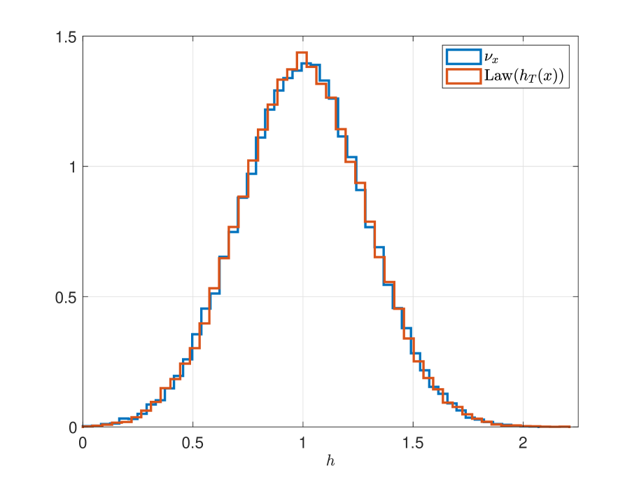
(a)

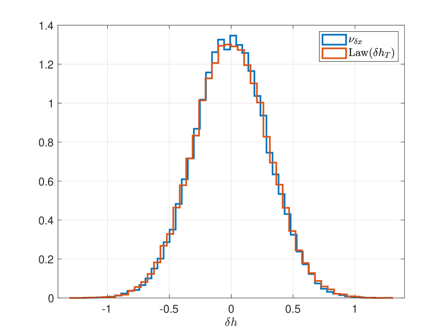
(b)

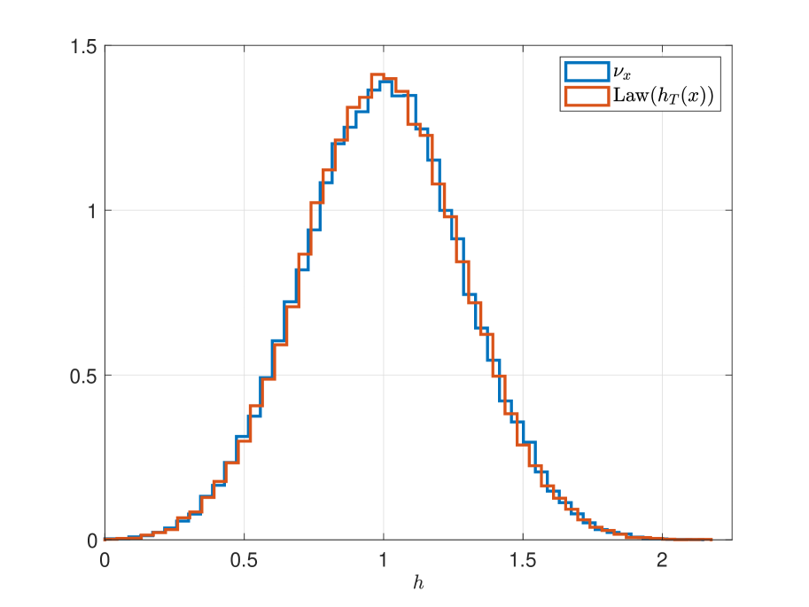
(c)

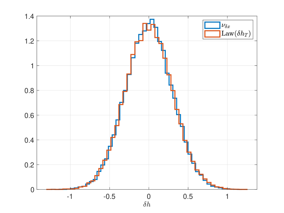
(d)

Figure 5. Plots of the histograms for $M=1000$ samples of the single-point statistics and two-point correlations of the film height, i.e. $h_{T}$ and $\delta h_{T}=h_{T}(x+\delta x)-h_{T}(x)$, for the Grün–Rumpf ((A),(B)) and the central difference ((C),(D)) discretizations compared to the reference measure, the conservative Brownian excursion $\nu_{N}$. The simulations were carried out with the following parameters: $N=50$, $\Delta t=10^{-10}$, $\beta=1$, $T=10^{-3}$, $\delta x=0.1$, and $h_{0}\equiv 1$.

11.2. Invariance of the measure $\nu_{N}$

In this subsection, we perform some numerical experiments to check the invariance of the measure $\nu_{N}$. We start by describing below a simple numerical procedure to sample from $\nu_{N}$.

Result: Realization of $\nu_{N}$

Sample discrete spatial white noise at temperature $\beta^{-1}$, i.e. a random $N$-dimensional vector of i.i.d. $\mathcal{N}(0,\beta^{-1}N\times\mathrm{Id})$-distributed random variables $dW_{N}$;

Project onto average zero vectors: $\mathop{}\!\mathup{d}W_{N}^{0}=\mathop{}\!\mathup{d}W_{N}-N^{-1}\sum_{i}\mathop{}\!\mathup{d}W_{N,i}$;

Integrate to get a discrete Brownian bridge: $W_{N,1}^{0}=0,\,W_{N,i}^{0}=W_{N,i-1}^{0}+N^{-1}\mathop{}\!\mathup{d}W_{N,i-1}^{0}$;

Project onto average $1$ vectors: $W_{N}=W_{N}^{0}-N^{-1}\left(\sum_{i}W_{N,i}^{0}\right)+1$;

if $\exists i$ s.t. $W_{N,i}<0$ then

       reject;

      

else

       accept;

      

end if

Algorithm 1 Sampling from $\nu_{N}$

We now integrate in time starting from $h_{0}\equiv 1$ according to the semi-implicit Euler–Maruyama algorithm described in (11.1) up to some large time $T\gg\Delta t$. Repeating this procedure, we obtain a large number of samples, $M\gg 1$, of the process at time $t=T$ which we compare to the samples of $\nu_{N}$ generated by Algorithm 1. Note that $T$ needs to be chosen to be larger than the typical relaxation time (to the invariant measure) of both discretizations. We found that $T=10^{-3}$ works well for this purpose. We compare both the single-point distributions and the two-point correlations, i.e. the law of $\delta h_{T}=h_{T}(x+\delta x)-h_{T}(x)$ for some $\frac{1}{N}=:\Delta x\ll\delta x\ll 1$. Due to the stationarity (in space) of the invariant measure the choice of $x\in\left[0,1\right]$ is irrelevant. We present the results of this experiment in Fig. 5.

11.3. Positivity, exit times, and entropic repulsion

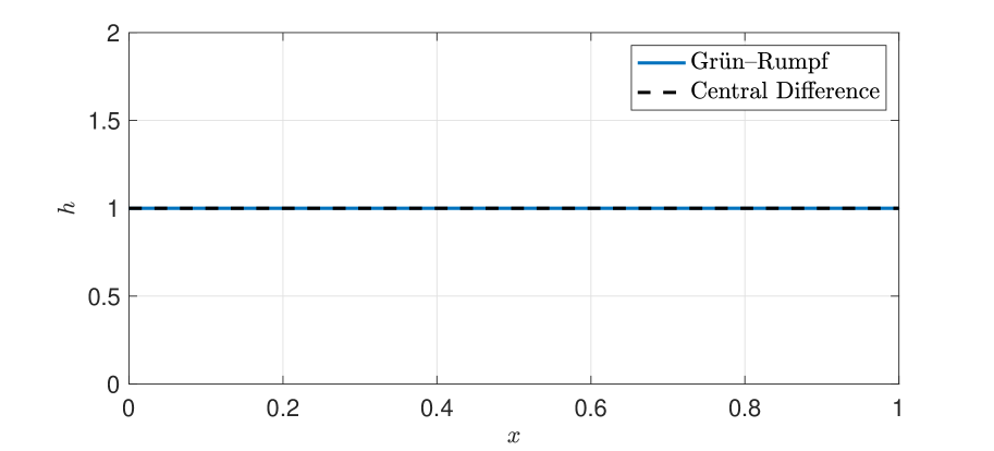
(a) $t=0$

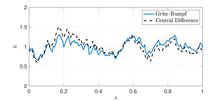
(b) $t\approx 1.64\times 10^{-4}$

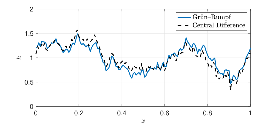
(c) $t\approx 3.28\times 10^{-4}$

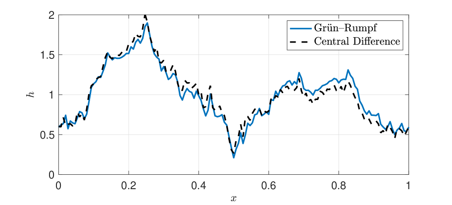
(d) $t\approx 4.92\times 10^{-4}$

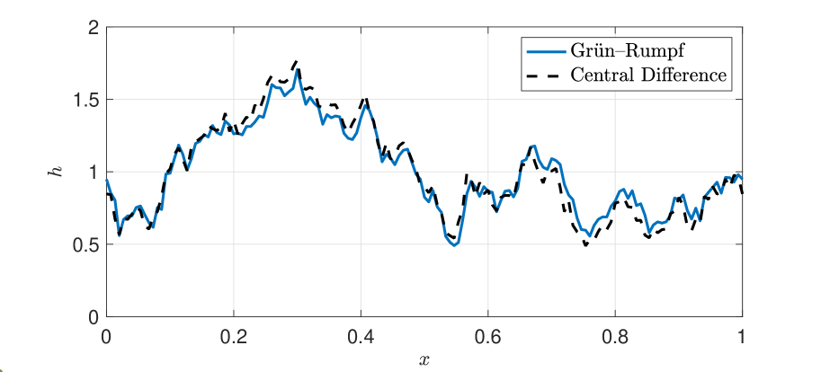
(e) $t\approx 6.56\times 10^{-4}$

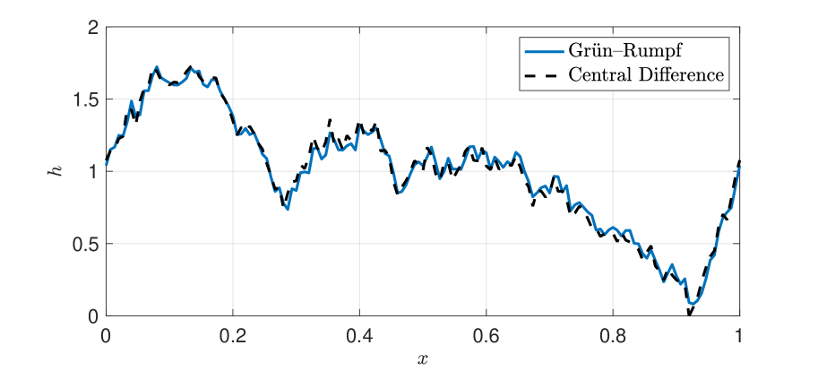
(f) $t\approx 8.2\times 10^{-4}$

Figure 6. Snapshots of the film height for the Grün–Rumpf and central difference discretizations at equally spaced time increments (time goes from (A) $\to$ (F)) for the same realization of the noise. As can be seen from the figures, the central difference discretization touches down (at $t_{*}\approx 8.2\times 10^{-4}$, see (F)) while the Grün–Rumpf discretization stays away from the boundary. The simulations were performed with the following parameters: $N=150$, $\Delta t=10^{-10}$, $\beta=1$, and $h_{0}\equiv 1$.

As shown in 8.4, under appropriate conditions on the initial datum, the Grün–Rumpf discretization stays away from the boundary $\partial\mathcal{M}_{N}$. On the other hand, one expects (see the discussion in Section 9) the central difference discretization to touch the boundary with probability 1. We provide some numerical evidence for these features of the two discretizations in Fig. 6. Indeed, for the same realization of the noise, the Grün–Rumpf discretization stays away from $0$, while the central difference discretization touches down.

We can provide stronger numerical evidence for the fact that the central difference discretization touches down by computing the mean exit time from $\mathcal{M}_{N}$ of the associated process. If this quantity is finite, this implies that the central difference discretization leaves $\mathcal{M}_{N}$, i.e. touches down, almost surely. Let $h^{h_{0}}_{t}$ be a solution of the central difference discretization of the stochastic thin-film equation (9.3) with initial condition $h_{0}\in\mathcal{M}_{N}$. Then, we define the exit time of $h_{t}^{h_{0}}$ from the interior to be

(11.2) $$\tau(h_{0}):=\inf\left\{t\geq 0:h^{h_{0}}_{t}\notin\mathcal{M}_{N}\right\}.$$

We take $h_{0}\equiv 1$ and set $\tau:=\tau(1)$. Then, we sample $\tau$ by running a Monte-Carlo simulation of (9.3) according to the time-stepping scheme described in (11.1). This time, instead of imposing reflecting boundary conditions, we stop the simulation as soon as we reach the boundary $\partial\mathcal{M}_{N}$, i.e. when the film touches down.  Fig. 7 shows the behavior of the mean exit time as $N$ grows. In particular, it seems that the mean exit time is finite and remains bounded as $N$ tends to infinity.

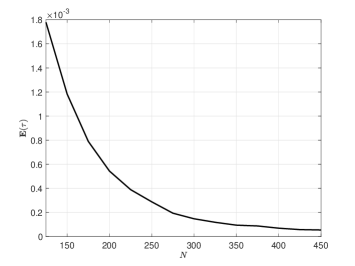
Figure 7. The dependence of the mean exit time of the central difference discretization on $N$. The simulations were performed with the following parameters: $\Delta t=10^{-10}$, $\beta=1$, $M=100$, and $h_{0}\equiv 1$.

In the final part of this subsection, we study numerically the positivity properties of the continuum conservative Brownian excursion $\nu$, i.e. its entropic repulsion. As has been mentioned before, our conservative Brownian excursion is qualitatively similar to the classical Brownian excursion from stochastic analysis. Moreover, it is known that the classical Brownian excursion features an entropic repulsion, in the sense that the single point distribution decays to $0$ at $0$. In fact, one can compute the single point statistics for the classical Brownian excursion $\left(Y_{t}\right)_{t\geq 0}$ explicitly (cf. [40, p.463]): For fixed $t\geq 0$ and $x,y>0$ such that $Y_{0}=x$ and $Y_{T}=y$ a.s., it takes the form

(11.3) $$p^{x,y}_{t}(z)=\frac{T}{t(T-t)}z\frac{I_{\frac{1}{2}}(\frac{xz}{t})I_{\frac{1}{2}}(\frac{zy}{T-t})}{I_{\frac{1}{2}}(\frac{xy}{T})}e^{-\frac{x^{2}+z^{2}}{2t}}e^{-\frac{z^{2}+y^{2}}{2(T-t)}}e^{\frac{x^{2}+y^{2}}{2T}}$$

where $I_{\frac{1}{2}}$ is the modified Bessel function of the first kind of order $\frac{1}{2}$. Notice that for $z\ll 1$, it holds that $I_{\frac{1}{2}}(z)\sim z^{\frac{1}{2}}$. From the above expression, it is clear that the distribution decays to $0$ quadratically as $z\to 0$. In  Fig. 8 we see that the single point distribution of our conservative Brownian excursion for $N\gg 1$ also exhibits quadratic decay at $0$.

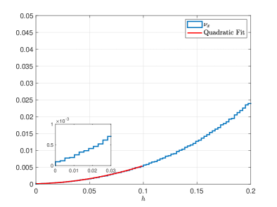
Figure 8. The entropic repulsion of the continuum conservative Brownian excursion $\nu$ as observed through the single point statistics of $\nu_{N}$ for $N$ large ($=2000$) obtained from $M=2\times 10^{5}$ samples. The single point distribution (in blue) decays quadratically as $h\to 0$ as can be seen by comparing it to the fitted curve (in red) $p(h)\approx 0.4704\times h^{2}$. The zoomed-in version of the histogram exhibits the fact that entropic repulsion is a feature of the continuum invariant measure; for finite but large $N$ the single point density is positive but small at $0$.

11.4. Convergence of the two discretizations

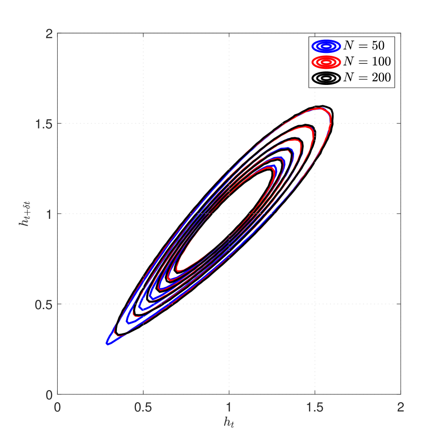
(a)

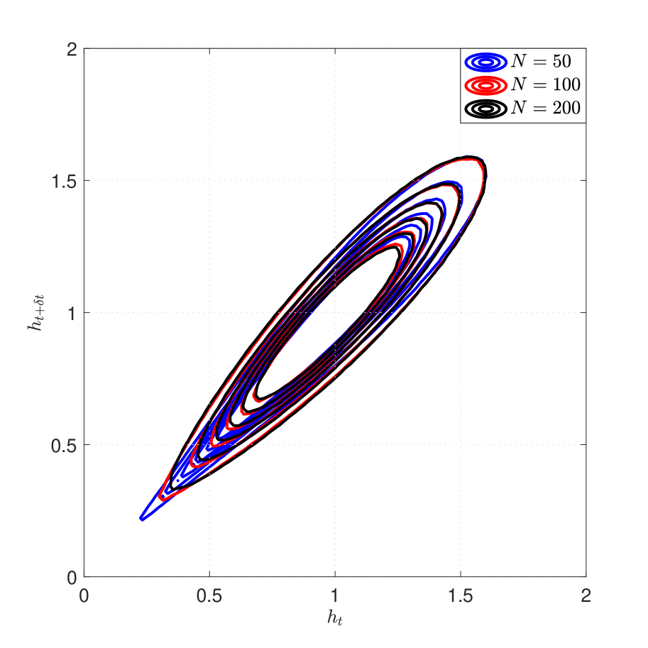
(b)

Figure 9. Level sets of the two-point (in time) distributions, i.e. the joint distributions of $h_{t}$ and $h_{t+\delta t}$, for (A) the Grün–Rumpf and (B) the central difference discretizations for $N=50,100,200$.

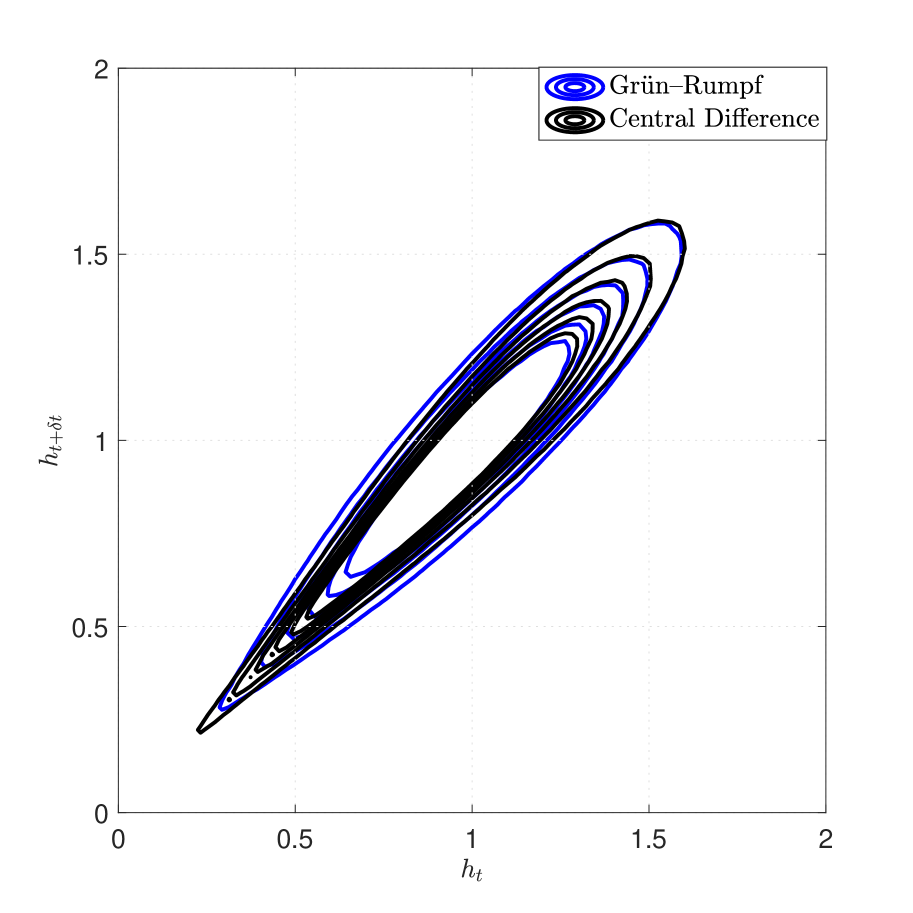
(a)

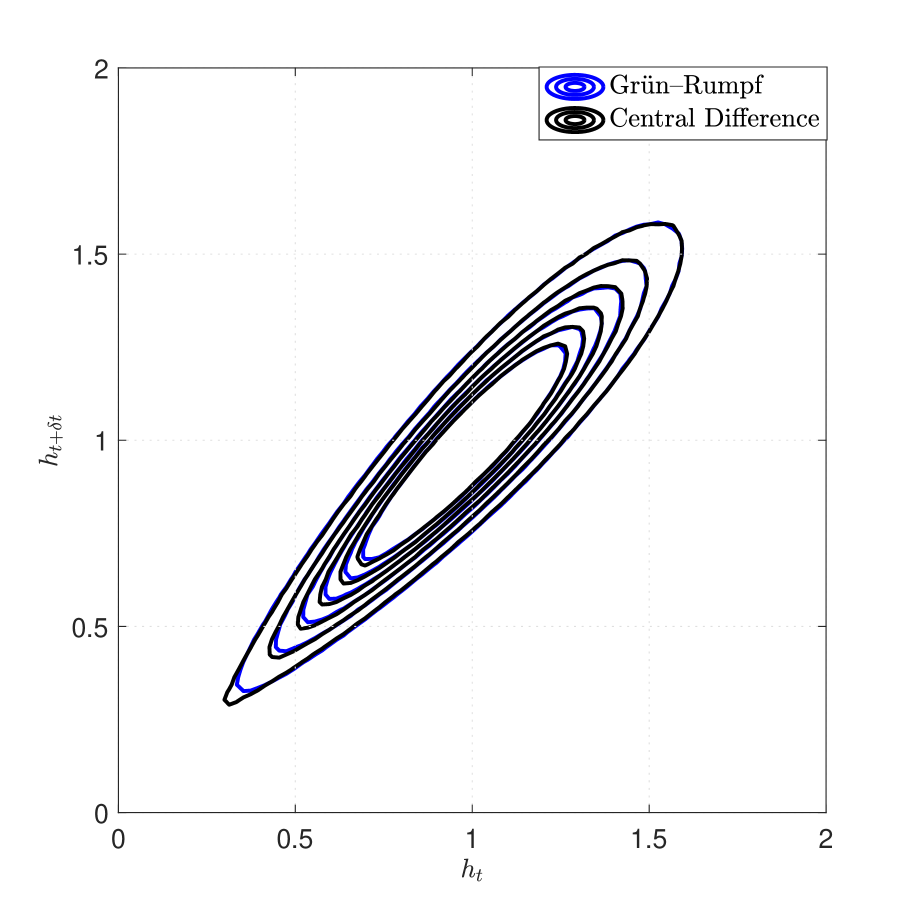
(b)

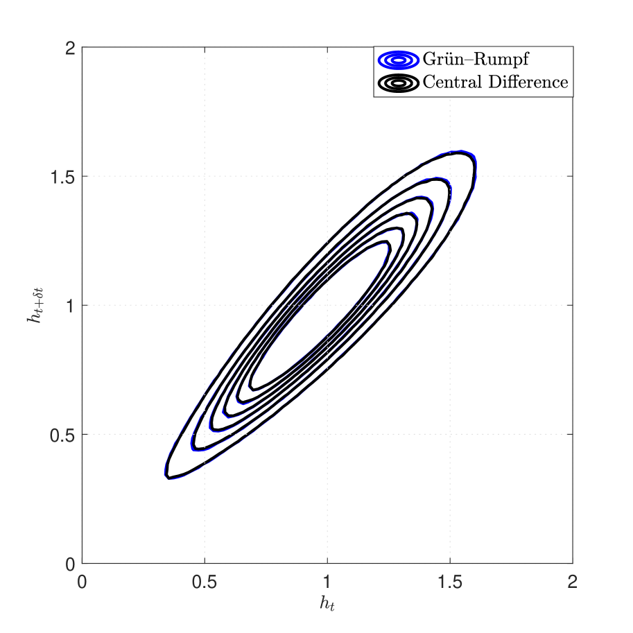
(c)

Figure 10. Comparisons of the level sets of the two-point (in time) distributions of the the Grün–Rumpf and the central difference discretizations for (A) $N=50$, (B) $N=100$, and (C) $N=200$.

As mentioned earlier in the paper, two different discretizations of a singular SPDE can converge to different limiting objects (cf. [25]). Thus, it would not be unreasonable to expect that the Grün–Rumpf and central difference discretizations of the thin-film equation with thermal noise have different continuum limits. However, numerical evidence seems to indicate that, at least started at equilibrium, the path space measures of the two discretizations converge to the same object.

We check this by sampling from $\nu_{N}$ using Algorithm 1 and then integrating in time with $h_{0}\sim\nu_{N}$ to some final time $T$. Repeating this process, we obtain a large number, $M\gg 1$, of samples. We can then compute the two-point (in time) distributions of both discretizations, i.e. the joint law of $h_{t}$ and $h_{t+\delta t}$ for some $\Delta t\ll\delta t\ll T$, for different values of $N$. One then observes that, as $N$ increases, the two discretizations seem to converge to each other. Note that since we start our simulations at the invariant measure and the underlying process is reversible the choice of $t\geq 0$ is irrelevant. We present the results of these experiments in Figs. 9 and 10.

Appendix A The thin-film equation with linear mobility in Lagrangian coordinates

Let

(A.1) $$z=\int_{0}^{X(z)}h(x)\mathop{}\!\mathup{d}x$$

then taking the derivative twice with respect to $z$ of (A.1) yields

(A.2) $$1=h(X(z))\frac{\mathop{}\!\mathup{d}missing}{\mathop{}\!\mathup{d}z}X(z)$$

as well as

(A.3) $$0=\partial_{x}h(X(z))\left(\frac{\mathop{}\!\mathup{d}missing}{\mathop{}\!\mathup{d}z}X(z)\right)^{2}+h(X(z))\frac{\mathop{}\!\mathup{d}^{2}}{\mathop{}\!\mathup{d}z^{2}}X(z).$$

Multiplying (A.3) with $h(X(z))^{2}$ and invoking (A.2) we end up with

(A.4) $$\partial_{x}h(X(z))=-h(X(z))^{3}\frac{\mathop{}\!\mathup{d}^{2}}{\mathop{}\!\mathup{d}z^{2}}X(z).$$

Hence we compute for the Dirichlet energy

(A.5) $$E(h) :=\frac{1}{2}\int_{0}^{1}(\partial_{x}h)^{2}\mathop{}\!\mathup{d}x=\frac{1}{2}\int_{0}^{1}(\partial_{x}h(X(z)))^{2}\frac{\mathop{}\!\mathup{d}missing}{\mathop{}\!\mathup{d}z}X(z)\mathop{}\!\mathup{d}z$$

(A.6) $$\stackrel{{\scriptstyle\eqref{formuladxh2}}}{{=}}\frac{1}{2}\int_{0}^{1}\left(h(X(z))^{3}\frac{\mathop{}\!\mathup{d}^{2}}{\mathop{}\!\mathup{d}z^{2}}X(z)\right)^{2}\frac{\mathop{}\!\mathup{d}missing}{\mathop{}\!\mathup{d}z}X(z)\mathop{}\!\mathup{d}z$$

(A.7) $$\stackrel{{\scriptstyle\eqref{formulah}}}{{=}}\frac{1}{2}\int_{0}^{1}\frac{\left(\frac{\mathop{}\!\mathup{d}^{2}}{\mathop{}\!\mathup{d}z^{2}}X(z)\right)^{2}}{\left(\frac{\mathop{}\!\mathup{d}missing}{\mathop{}\!\mathup{d}z}X(z)\right)^{5}}\mathop{}\!\mathup{d}z$$

(A.8) $$=:E(X).$$

Moreover, for some $\delta X$ we compute

(A.9) $$\mathrm{diff}E|_{X}.\delta X =\frac{1}{2}\int_{0}^{1}2\frac{\frac{\mathop{}\!\mathup{d}^{2}}{\mathop{}\!\mathup{d}z^{2}}X(z)}{\left(\frac{\mathop{}\!\mathup{d}missing}{\mathop{}\!\mathup{d}z}X(z)\right)^{5}}\frac{\mathop{}\!\mathup{d}^{2}}{\mathop{}\!\mathup{d}z^{2}}(\delta X(z))-5\frac{\left(\frac{\mathop{}\!\mathup{d}^{2}}{\mathop{}\!\mathup{d}z^{2}}X(z)\right)^{2}}{\left(\frac{\mathop{}\!\mathup{d}missing}{\mathop{}\!\mathup{d}z}X(z)\right)^{6}}\frac{\mathop{}\!\mathup{d}missing}{\mathop{}\!\mathup{d}z}(\delta X(z))\mathop{}\!\mathup{d}z$$

(A.10) $$=\int_{0}^{1}\left(\frac{\mathop{}\!\mathup{d}^{2}}{\mathop{}\!\mathup{d}z^{2}}\left(\frac{\frac{\mathop{}\!\mathup{d}^{2}}{\mathop{}\!\mathup{d}z^{2}}X(z)}{\left(\frac{\mathop{}\!\mathup{d}missing}{\mathop{}\!\mathup{d}z}X(z)\right)^{5}}\right)+\frac{5}{2}\frac{\mathop{}\!\mathup{d}missing}{\mathop{}\!\mathup{d}z}\left(\frac{\left(\frac{\mathop{}\!\mathup{d}^{2}}{\mathop{}\!\mathup{d}z^{2}}X(z)\right)^{2}}{\left(\frac{\mathop{}\!\mathup{d}missing}{\mathop{}\!\mathup{d}z}X(z)\right)^{6}}\right)\right)\delta X(z)\mathop{}\!\mathup{d}z.$$

This, as usual, gives rise to the $L^{2}$-gradient flow

(A.11) $$\partial_{t}X =-\partial_{z}^{2}\left(\frac{\partial_{z}^{2}X}{\left(\partial_{z}X\right)^{5}}\right)-\frac{5}{2}\partial_{z}\left(\frac{\left(\partial_{z}^{2}X\right)^{2}}{\left(\partial_{z}X\right)^{6}}\right)$$

(A.12) $$=\frac{1}{4}\partial_{z}^{3}\left(\partial_{z}X\right)^{-4}-\frac{5}{8}\partial_{z}\left(\partial_{z}\left(\partial_{z}X\right)^{-2}\right)^{2}.$$

Appendix B Computing the change of coordinates

B.1. The dual metric in coordinates

Let the setting be as in the beginning of Section 6. As usual, we define the musical isomorphism via

(B.1) $$T^{*}\mathcal{M}\to T\mathcal{M},\omega\to\omega^{\sharp}$$

where

(B.2) $$\omega.\dot{h}=g\left(\omega^{\sharp},\dot{h}\right)$$

for all $\dot{h}\in T\mathcal{M}$. This gives rise to the dual metric $g^{\prime}$ on $T^{*}\mathcal{M}\otimes T^{*}\mathcal{M}$ via

(B.3) $$g^{\prime}\left(\omega,\omega^{\prime}\right):=g\left(\omega^{\sharp},\omega^{\prime\sharp}\right)$$

for all $\omega,\omega^{\prime}\in T^{*}\mathcal{M}$. Let $g^{\prime\alpha\alpha^{\prime}}$ and $g_{\alpha\alpha^{\prime}}$ be the representation of $g^{\prime}$ respectively $g$ in the coordinates $\left(\varphi^{\alpha}\right)_{\alpha}$ and let $\ell,\ell^{\prime}$ be covectors and $\tau,\tau^{\prime}$ be vectors that are related by

(B.4) $$\ell_{\alpha}=g_{\alpha\alpha^{\prime}}\tau^{\alpha^{\prime}},\quad\ell^{\prime}_{\alpha}=g_{\alpha\alpha^{\prime}}\tau^{\prime\alpha^{\prime}}.$$

Then by definition of (B.3) and by (B.4), we have

(B.5) $$g_{\alpha\alpha^{\prime}}\tau^{\alpha}\tau^{\prime\alpha^{\prime}}=g^{\prime\alpha\alpha^{\prime}}\ell_{\alpha}\ell^{\prime}_{\alpha^{\prime}}$$

and thus we see that $g^{\prime\alpha\alpha^{\prime\prime}}g_{\alpha^{\prime\prime}\alpha^{\prime}}=\delta_{\alpha\alpha^{\prime}}$ such that finally

(B.6) $$g^{\prime\alpha\alpha^{\prime}}=g^{\alpha\alpha^{\prime}}.$$

Moreover, by (B.3) and (B.6), we see that for $\zeta,\zeta^{\prime}$ sufficiently smooth functions on $\mathcal{M}$ we have

(B.7) $$g\left(\nabla\zeta,\nabla\zeta^{\prime}\right)=g^{\prime}\left(\mathrm{diff}\zeta,\mathrm{diff}\zeta^{\prime}\right)=g^{\alpha\alpha^{\prime}}\partial_{\alpha}\zeta\partial_{\alpha^{\prime}}\zeta^{\prime}.$$

B.2. Explicit formulae for partial derivatives

For some function $f:\mathcal{M}_{N}\to{\mathbb{R}}$ we have

(B.8) $$\partial_{i}f(h)=\frac{\mathop{}\!\mathup{d}missing}{\mathop{}\!\mathup{d}\varepsilon}\Bigr{|}_{\varepsilon=0}f(h+\varepsilon\hat{\varphi}_{i})$$

as well as

(B.9) $$\partial_{\alpha}f(h)=\frac{\mathop{}\!\mathup{d}missing}{\mathop{}\!\mathup{d}\varepsilon}\Bigr{|}_{\varepsilon=0}f(h+\varepsilon\overline{\varphi}_{\alpha}).$$

Appendix C Computation of the numerical mobility

We restrict ourselves to mobility functions of the form $M(h)=h^{m}$. Then we compute

(C.1) $$g_{\alpha\alpha}(h) =\frac{1}{m-1}\frac{\left(h^{\alpha-}\right)^{1-m}-\left(h^{\alpha+}\right)^{1-m}}{h^{\alpha+}-h^{\alpha-}}$$

(C.2) $$=\frac{1}{m-1}\frac{1}{h^{\alpha+}-h^{\alpha-}}\frac{\left(h^{\alpha+}\right)^{m-1}-\left(h^{\alpha-}\right)^{m-1}}{\left(h^{\alpha-}\right)^{m-1}\left(h^{\alpha+}\right)^{m-1}}$$

(C.3) $$=\frac{1}{m-1}\frac{1}{h^{\alpha+}-h^{\alpha-}}\frac{\sum_{k=1}^{\infty}\binom{m-1}{k}\left(h_{\alpha-}\right)^{m-1-k}(h^{\alpha+}-h^{\alpha-})^{k}}{\left(h^{\alpha-}\right)^{m-1}\left(h^{\alpha+}\right)^{m-1}}$$

(C.4) $$=\frac{1}{m-1}\frac{\sum_{k=1}^{\infty}\binom{m-1}{k}\left(h^{\alpha-}\right)^{m-1-k}(h^{\alpha+}-h^{\alpha-})^{k-1}}{\left(h^{\alpha-}\right)^{m-1}\left(h^{\alpha+}\right)^{m-1}}.$$

In particular, this yields for $m=3$

(C.5) $$g_{\alpha\alpha}(h)=\frac{1}{2}\frac{h^{\alpha-}+h^{\alpha+}}{\left(h^{\alpha-}\right)^{2}\left(h^{\alpha+}\right)^{2}}$$

and hence

(C.6) $$g^{\alpha\alpha}(h)=2\frac{\left(h^{\alpha-}\right)^{2}\left(h^{\alpha+}\right)^{2}}{h^{\alpha-}+h^{\alpha+}}.$$

Moreover, for the Itô-correction term we are left with computing

(C.7) $$\partial_{\alpha^{\prime}}g^{\alpha^{\prime}\alpha}(h)=-g^{\gamma\gamma^{\prime}}(h)\partial_{\gamma}g_{\gamma^{\prime}\alpha^{\prime}}(h)g^{\alpha^{\prime}\alpha}(h)$$

and using (B.2) we compute the derivative of the metric tensor via

(C.8) $$\partial_{\gamma}g_{\gamma^{\prime}\alpha^{\prime}}(h)=-\delta_{\gamma^{\prime}\alpha^{\prime}}\mathchoice{{\vbox{\hbox{$\textstyle-$ }}\kern-7.83337pt}}{{\vbox{\hbox{$\scriptstyle-$ }}\kern-5.90005pt}}{{\vbox{\hbox{$\scriptscriptstyle-$ }}\kern-4.75003pt}}{{\vbox{\hbox{$\scriptscriptstyle-$ }}\kern-4.25003pt}}\!\int_{I_{\alpha^{\prime}}}\frac{M^{\prime}(h)}{M(h)^{2}}\overline{\varphi}_{\gamma}\mathop{}\!\mathup{d}x.$$

By the diagonal structure of $g(h)$ it is enough to compute

(C.9) $$\partial_{\alpha}g_{\alpha\alpha}(h)=N^{\frac{3}{2}}\frac{\frac{1}{M(h^{\alpha+})}+\frac{1}{M(h^{\alpha-})}-2g_{\alpha\alpha}(h)}{h^{\alpha+}-h^{\alpha-}}$$

where we used integration by parts which in the case $m=3$ yields

(C.10) $$\partial_{\alpha}g_{\alpha\alpha}(h) =N^{\frac{3}{2}}\frac{\left(h^{\alpha-}\right)^{-3}+\left(h^{\alpha+}\right)^{-3}-\frac{h^{\alpha-}+h^{\alpha+}}{\left(h^{\alpha-}\right)^{2}\left(h^{\alpha+}\right)^{2}}}{h^{\alpha+}-h^{\alpha-}}$$

(C.11) $$=N^{\frac{3}{2}}\frac{\left(h^{\alpha-}\right)^{-2}(\left(h^{\alpha-}\right)^{-1}-\left(h^{\alpha+}\right)^{-1})+\left(h^{\alpha+}\right)^{-2}(\left(h^{\alpha+}\right)^{-1}-\left(h^{\alpha-}\right)^{-1})}{h^{\alpha+}-h^{\alpha-}}$$

(C.12) $$=N^{\frac{3}{2}}\left(\frac{1}{\left(h^{\alpha-}\right)^{3}h^{\alpha+}}-\frac{1}{\left(h^{\alpha+}\right)^{3}h^{\alpha-}}\right).$$

Hence, for $m=3$, we have

(C.14) $$\partial_{\alpha^{\prime}}g^{\alpha^{\prime}\alpha}(h)=N^{\frac{3}{2}}4h^{i}h^{i+1}\frac{h^{i}-h^{i+1}}{h^{i}+h^{i+1}}.$$

Appendix D An integral inequality

Lemma D.1.

Let u(t) be positive and bounded for $t\in\left[0,T\right]$. Let $0\leq\gamma<\infty$. Then, if

(D.1) $$u(t)\leq u(0)+Ct+C\int_{0}^{t}u^{\gamma}(s)\mathop{}\!\mathup{d}s$$

for some constant $C$, we have for $\gamma=1$

(D.2) $$u(t)\leq\left(u(0)+1\right)e^{Ct}$$

and for $\gamma\neq 1$

(D.3) $$u(t)\leq\left(\left(u(0)+CT\right)^{1-\gamma}+(1-\gamma)Ct\right)^{\frac{1}{1-\gamma}}.$$

Proof.

For $\gamma=1$ we note that we can write (D.1) as

(D.4) $$u(t)+1\leq u(0)+1+C\int_{0}^{t}u(s)+1\mathop{}\!\mathup{d}s$$

and then apply Gronwall’s inequality to get the assertion.

If $\gamma<1$ then we set $X(t):=\int_{0}^{t}u^{\gamma}(s)\mathop{}\!\mathup{d}s$ and hence

(D.5) $$\frac{\mathop{}\!\mathup{d}missing}{\mathop{}\!\mathup{d}t}X(t)=u^{\gamma}(t)\stackrel{{\scriptstyle\eqref{gamma1}}}{{\leq}}\left(u(0)+Ct+CX(t)\right)^{\gamma}$$

which implies

(D.6) $$\frac{\mathop{}\!\mathup{d}missing}{\mathop{}\!\mathup{d}t}\left(u(0)+CT+CX(t)\right)\leq C\left(u(0)+CT+CX(t)\right)^{\gamma}.$$

The differential inequality (D.6) further yields

(D.7) $$\frac{\mathop{}\!\mathup{d}missing}{\mathop{}\!\mathup{d}t}\left(u(0)+CT+CX(t)\right)^{1-\gamma}\leq C_{\gamma}$$

for $C_{\gamma}:=(1-\gamma)C$ and since $X(0)=0$ we have by integrating that

(D.8) $$\left(u(0)+CT+CX(t)\right)^{1-\gamma}\leq\left(u(0)+CT\right)^{1-\gamma}+C_{\gamma}t.$$

By taking the inverse and appealing again to the assumption (D.1) we get the desired estimate. ∎

References

- [1] J.-D. Benamou and Y. Brenier. A computational fluid mechanics solution to the Monge-Kantorovich mass transfer problem. Numer. Math., 84(3):375–393, 2000.
- [2] E. Beretta, M. Bertsch, and R. Dal Passo. Nonnegative solutions of a fourth-order nonlinear degenerate parabolic equation. Arch. Rational Mech. Anal., 129(2):175–200, 1995.
- [3] F. Bernis. Finite speed of propagation and continuity of the interface for thin viscous flows. Adv. Differential Equations, 1(3):337–368, 1996.
- [4] F. Bernis and A. Friedman. Higher order nonlinear degenerate parabolic equations. J. Differential Equations, 83(1):179–206, 1990.
- [5] A. L. Bertozzi and M. Pugh. The lubrication approximation for thin viscous films: regularity and long-time behavior of weak solutions. Comm. Pure Appl. Math., 49(2):85–123, 1996.
- [6] M. Bertsch, R. Dal Passo, H. Garcke, and G. Grün. The thin viscous flow equation in higher space dimensions. Adv. Differential Equations, 3(3):417–440, 1998.
- [7] F. Cornalba. A priori positivity of solutions to a non-conservative stochastic thin-film equation. arXiv preprint arXiv:1811.07826, 2018.
- [8] R. Dal Passo, H. Garcke, and G. Grün. On a fourth-order degenerate parabolic equation: global entropy estimates, existence, and qualitative behavior of solutions. SIAM J. Math. Anal., 29(2):321–342, 1998.
- [9] R. Dal Passo, L. Giacomelli, and G. Grün. A waiting time phenomenon for thin film equations. Ann. Scuola Norm. Sup. Pisa Cl. Sci. (4), 30(2):437–463, 2001.
- [10] K. Dareiotis, B. Gess, M. V. Gnann, and G. Grün. Non-negative Martingale Solutions to the Stochastic Thin-Film Equation with Nonlinear Gradient Noise. arXiv e-prints, page arXiv:2012.04356, Dec. 2020.
- [11] B. Davidovitch, E. Moro, and H. A. Stone. Spreading of viscous fluid drops on a solid substrate assisted by thermal fluctuations. Physical review letters, 95(24):244505, 2005.
- [12] D. A. Dawson and J. Gärtner. Large deviations from the McKean-Vlasov limit for weakly interacting diffusions. Stochastics, 20(4):247–308, 1987.
- [13] J.-D. Deuschel and G. Giacomin. Entropic repulsion for massless fields. Stochastic Process. Appl., 89(2):333–354, 2000.
- [14] M. A. Durán-Olivencia, R. S. Gvalani, S. Kalliadasis, and G. A. Pavliotis. Instability, rupture and fluctuations in thin liquid films: theory and computations. J. Stat. Phys., 174(3):579–604, 2019.
- [15] J. Fischer. Optimal lower bounds on asymptotic support propagation rates for the thin-film equation. J. Differential Equations, 255(10):3127–3149, 2013.
- [16] J. Fischer. Upper bounds on waiting times for the thin-film equation: the case of weak slippage. Arch. Ration. Mech. Anal., 211(3):771–818, 2014.
- [17] J. Fischer and G. Grün. Existence of positive solutions to stochastic thin-film equations. SIAM J. Math. Anal., 50(1):411–455, 2018.
- [18] M. I. Freidlin and A. D. Wentzell. Random perturbations of dynamical systems, volume 260 of Grundlehren der Mathematischen Wissenschaften [Fundamental Principles of Mathematical Sciences]. Springer-Verlag, New York, 1984. Translated from the Russian by Joseph Szücs.
- [19] P. K. Friz and M. Hairer. A course on rough paths. Universitext. Springer, Cham, 2014. With an introduction to regularity structures.
- [20] B. Gess and M. V. Gnann. The stochastic thin-film equation: existence of nonnegative martingale solutions. Stochastic Process. Appl., 130(12):7260–7302, 2020.
- [21] L. Giacomelli and F. Otto. Rigorous lubrication approximation. Interfaces Free Bound., 5(4):483–529, 2003.
- [22] G. Grün. Degenerate parabolic differential equations of fourth order and a plasticity model with non-local hardening. Z. Anal. Anwendungen, 14(3):541–574, 1995.
- [23] G. Grün, K. Mecke, and M. Rauscher. Thin-film flow influenced by thermal noise. J. Stat. Phys., 122(6):1261–1291, 2006.
- [24] G. Grün and M. Rumpf. Nonnegativity preserving convergent schemes for the thin film equation. Numer. Math., 87(1):113–152, 2000.
- [25] M. Hairer and J. Maas. A spatial version of the Itô-Stratonovich correction. Ann. Probab., 40(4):1675–1714, 2012.
- [26] M. Hairer, J. Maas, and H. Weber. Approximating rough stochastic PDEs. Comm. Pure Appl. Math., 67(5):776–870, 2014.
- [27] M. Hairer and H. Weber. Large deviations for white-noise driven, nonlinear stochastic PDEs in two and three dimensions. Ann. Fac. Sci. Toulouse Math. (6), 24(1):55–92, 2015.
- [28] N. Ikeda and S. Watanabe. Stochastic differential equations and diffusion processes, volume 24 of North-Holland Mathematical Library. North-Holland Publishing Co., Amsterdam; Kodansha, Ltd., Tokyo, second edition, 1989.
- [29] I. Karatzas and S. E. Shreve. Brownian motion and stochastic calculus, volume 113 of Graduate Texts in Mathematics. Springer-Verlag, New York, 1988.
- [30] H. Knüpfer and N. Masmoudi. Darcy’s flow with prescribed contact angle: well-posedness and lubrication approximation. Arch. Ration. Mech. Anal., 218(2):589–646, 2015.
- [31] R. Kohn, F. Otto, M. G. Reznikoff, and E. Vanden-Eijnden. Action minimization and sharp-interface limits for the stochastic Allen-Cahn equation. Comm. Pure Appl. Math., 60(3):393–438, 2007.
- [32] E. Lifshitz and L. P. P. (Auth.). Statistical Physics. Theory of the Condensed State. 1980.
- [33] S. Metzger and G. Grün. Existence of nonnegative solutions to stochastic thin-film equations in two space dimensions, 2021.
- [34] A. Mielke, M. A. Peletier, and D. R. M. Renger. On the relation between gradient flows and the large-deviation principle, with applications to Markov chains and diffusion. Potential Anal., 41(4):1293–1327, 2014.
- [35] B. Øksendal. Stochastic differential equations. Universitext. Springer-Verlag, Berlin, sixth edition, 2003. An introduction with applications.
- [36] F. Otto. Lubrication approximation with prescribed nonzero contact angle. Comm. Partial Differential Equations, 23(11-12):2077–2164, 1998.
- [37] F. Otto. The geometry of dissipative evolution equations: the porous medium equation. Comm. Partial Differential Equations, 26(1-2):101–174, 2001.
- [38] F. Otto and H. Weber. Quasilinear SPDEs via rough paths. Arch. Ration. Mech. Anal., 232(2):873–950, 2019.
- [39] G. A. Pavliotis. Stochastic processes and applications, volume 60 of Texts in Applied Mathematics. Springer, New York, 2014. Diffusion processes, the Fokker-Planck and Langevin equations.
- [40] D. Revuz and M. Yor. Continuous martingales and Brownian motion, volume 293 of Grundlehren der Mathematischen Wissenschaften [Fundamental Principles of Mathematical Sciences]. Springer-Verlag, Berlin, third edition, 1999.
- [41] M. Sauerbrey. Martingale solutions to the stochastic thin-film equation in two dimensions, 2021.
- [42] K. Twardowska and A. Nowak. On the relation between the Itô and Stratonovich integrals in Hilbert spaces. Ann. Math. Sil., (18):49–63, 2004.
- [43] C. Villani. Topics in optimal transportation, volume 58 of Graduate Studies in Mathematics. American Mathematical Society, Providence, RI, 2003.
- [44] L. Zambotti. A reflected stochastic heat equation as symmetric dynamics with respect to the 3-d Bessel bridge. J. Funct. Anal., 180(1):195–209, 2001.
- [45] L. Zambotti. A conservative evolution of the Brownian excursion. Electron. J. Probab., 13:no. 37, 1096–1119, 2008.
- [46] L. Zhornitskaya and A. L. Bertozzi. Positivity-preserving numerical schemes for lubrication-type equations. SIAM J. Numer. Anal., 37(2):523–555, 2000.