Remeasuring the anomalously enhanced $B(E2;2^{+}\rightarrow 1^{+})$ in ${}^{8}\mathrm{Li}$

Abstract

The large reported $E2$ strength between the $2^{+}$ ground state and $1^{+}$ first excited state of $\isotope[8]{Li}$, $B(E2;2^{+}\rightarrow 1^{+})=55(15)\,e^{2}{\mathrm{fm}}^{4}$, presents a puzzle. Unlike in neighboring $A=7\text{--}9$ isotopes, where enhanced $E2$ strengths may be understood to arise from deformation as rotational in-band transitions, the $2^{+}\rightarrow 1^{+}$ transition in ⁸Li cannot be understood in any simple way as a rotational in-band transition. Moreover, the reported strength exceeds ab initio predictions by an order of magnitude. In light of this discrepancy, we revisited the Coulomb excitation measurement of this strength, now using particle-$\gamma$ coincidences, yielding a revised $B(E2;2^{+}\rightarrow 1^{+})$ of $19(^{+7}_{-6})(2)$ e²fm⁴. We explore how this value compares to what might be expected in the limits of rotational modesl. While the present value is about a factor of three smaller than previously reported, it remains anomalously enhanced.

I Introduction

Large $E2$ transition strengths found in the $A=7-9$ mass region [1, 2] suggest that these nuclei are significantly deformed, which gives rise to rotational structure as a dominant feature in the low-lying spectrum [3, 4]. The strong transitions between the ground state and first excited state in $\isotope[7]{Li}$, $\isotope[7]{Be}$, and $\isotope[9]{Be}$, or between excited states in $\isotope[8]{Be}$ [5], are interpreted as in-band rotational transitions. This deformation, in turn, is understood to arise from cluster molecular structure [6, *vonoertzen1997:be-alpha-rotational, 8, 9, 10, 11], e.g., with $\isotope[7]{Be}$ as a $\isotope[3]{He}+\isotope[4]{He}$ dimer, and the heavier $\isotope{Be}$ isotopes as $\isotope[4]{He}+\isotope[4]{He}$ plus neutrons.

In general, $E2$ strengths provide a probe of nuclear structure and its evolution [12]. For light $p$-shell nuclei, which are accessible to ab initio nuclear theory by a variety of approaches, ab initio calculations can provide qualitative insight into the structural origin of the $E2$ strengths [13, 14, 15, 16]. Meanwhile, experimental measurements can provide quantitative validation of the ability of calculations to faithfully describe the nuclear system [17].

Taken in this light, the large reported $E2$ strength between the $2^{+}$ ground state and $1^{+}$ first excited state of $\isotope[8]{Li}$, $B(E2;2^{+}\rightarrow 1^{+})=55(15)\,e^{2}{\mathrm{fm}}^{4}$ [18], presents a puzzle. This strength corresponds to $\sim 58$ Weisskopf units, which would be considered collective even in much heavier mass regions. The $M1$ strength for the $2^{+}_{1}\rightarrow 1^{+}_{1}$ transition can be deduced from the measured lifetime of this transition due to the dominance of the $M1$ component. The measured lifetime of the $1^{+}_{1}$ level was measured previously by the Doppler-shift attenuation method [19, 20]. The large value of the corresponding $M1$ transition strength is interesting in its own right, but we focus on the $E2$ component, which give complementary information to the $M1$ transition strength. As the $2^{+}_{1}\rightarrow 1^{+}_{1}$ transition in ⁸Li is dominated by the $M1$ component, we have chosen to use the technique of Coulomb excitation to selectively measure the $E2$ transition strength.

It is not unexpected that $\isotope[8]{Li}$ would be deformed. For instance, the ground state of the mirror nuclide $\isotope[8]{B}$ is suggested to have proton halo structure [21, 22, 23, 24] as a deformed $\isotope[7]{Be}$ core, with a loosely-bound proton in a spatially-extended molecular orbital [25]. The ground-state spectroscopic quadrupole moment of $\isotope[8]{Li}$ is similar in magnitude to those of its deformed neighbors [26].

Nonetheless, an enhanced $2^{+}\rightarrow 1^{+}$ transition cannot be easily understood as an in-band rotational transition, like the transitions in neighboring nuclei. As least in a conventional axially-symmetric rotational picture [27, 28], if the $2^{+}$ ground state is the band head of a $K=2$ band, there is no $1^{+}$ band member, and the transition to the $1^{+}$ excited state is at most an interband transition (between $K=2$ and $K=1$ band heads).

Moreover the reported strength exceeds ab initio Green’s function Monte Carlo (GFMC) predictions [15] by nearly two orders of magnitude, despite the same calculations predicting a result for the quadrupole moment of the $2^{+}$ ground state, which is in line with experiment [26]. In this paper, we present ab initio no-core shell model (NCSM) calculations of the type presented in Ref. [29], with various interactions, which are likewise inconsistent with the reported $E2$ enhancement. Although the absolute scale of $E2$ strengths is poorly convergent in NCSM calculations, robust and meaningful predictions may be obtained by calibration [30] to the experimentally-known electric quadrupole moment.

The large reported $E2$ strength in $\isotope[8]{Li}$ [18] was measured by Coulomb excitation with a radioactive beam of $\isotope[8]{Li}$, where the inelastically-scattered $\isotope[8]{Li}$ nuclei were detected by measuring their energy using a $\isotope{Si}$ detector. Such an experiment is ostensibly susceptible to events coming from ⁸Li that is produced in its excited state in the primary reaction rather than those coming from the Coulomb excitation of ⁸Li in the secondary target, which would result in an inflated measured Coulomb-excitation cross section and thus the extracted $E2$ strength. To eliminate such a possible source of error, we revisit this radioactive-beam Coulomb-excitation measurement, but now with gamma-ray detection capability, to impose a coincidence requirement between the detection of the inelastically-scattered $\isotope[8]{Li}$ nucleus and the $1^{+}\rightarrow 2^{+}$ deexcitation gamma ray. We use an array of high-efficiency $\isotope{La}\isotope{Br}_{3}$ gamma-ray detectors, in coincidence with a $\isotope{Si}$ particle detector centered on the secondary target. While we measure a smaller value than previously reported, the change is not sufficient to bring experiment in line with current theoretical understanding of the structure.

We first outline the present radioactive beam experiment with the TwinSol low-energy radioactive nuclear beam apparatus at the University of Notre Dame Nuclear Science Laboratory [31] (Sec. II) and detail the subsequent analysis used to extract the $2^{+}\rightarrow 1^{+}$ strength from Coulomb excitation (Sec. III), including an assessment of two-step and other possible contributions. We then discuss this strength in the context of rotational and ab initio descriptions (Sec. IV). These results were reported in part in Ref. [32].

II Experiment

In order to produce a beam of [8]Li, the 10 MV Tandem Van De Graaff at the University of Notre Dame Nuclear Science Laboratory (NSL) was used to accelerate a ${4.5}\,{e{\mathrm{\mu A}}}$ beam of [7]Li $3^{+}$ ions to ${26}\,{{\mathrm{MeV}}}$. This beam was steered to a production gas cell, which had a ${12}\,{{\mathrm{\mu m}}}$ thick [9]Be foil placed on the downstream side of the gas cell to serve as the production target. The gas cell was filled with ${300}\,{\mathrm{Torr}}$ of He gas to help cool the [9]Be target and a ${4}\,{{\mathrm{\mu m}}}$ Ti foil on the upstream side of the gas cell was used to contain the gas. The [8]Li beam was produced by the [9]Be([7]Li,[8]Be)[8]Li reaction at an energy of ${22.7(5)}\,{{\mathrm{MeV}}}$ (80% of the Coulomb barrier), along with other isotopes produced by competing reactions. This cocktail beam was sent into the TwinSol apparatus [31]. TwinSol consists of two superconducting solenoid magnets that are used as magnetic lenses to focus the radioactive beam of interest and eliminate contaminants. More details on how the TwinSol apparatus was used in this experiment are given in Ref. [17]. The first of these two solenoids was set to ${2.43}\,{\mathrm{T}}$ to best focus the [8]Li beam through a ${9}\,{{\mathrm{mm}}}$ diameter collimator placed between the solenoids, which eliminated the majority of the contaminants. The second solenoid was set to ${1.40}\,{\mathrm{T}}$, to refocus the [8]Li beam after it had passed through the collimator.

After exiting TwinSol, the [8]Li beam was sent into our scattering chamber. The first element the beam encountered was a ${9}\,{{\mathrm{mm}}}$ radius collimator, to eliminate divergent aspects of the beam and define the beam spot. The collimator and the experimental setup is shown in Fig. 1. Directly downstream of the collimator was a target ladder with a ${1}\,{{\mathrm{\mu m}}}$ thick [197]Au target, an empty frame, and a Si surface barrier detector for determining beam purity. During beam development, the beam was sent onto the surface barrier detector for particle identification and the final beam components were identified as being ${98}\,{\%}$ [8]Li with [7]Be and scattered [7]Li making up the majority of the contaminants. The optimized radioactive beam was sent onto the the gold foil for the duration of the experiment. Placed ${34.6}\,{{\mathrm{mm}}}$ downstream from the gold foil, a ${1000}\,{{\mathrm{\mu m}}}$-thick S7 annular Si detector, made by Micron Semiconductor Limited [33], was used to measured the beam that scattered from the [197]Au target in the angular range of ${20.6}^{\circ}$ - ${45.3}^{\circ}$ degrees. The upstream side of the Si detector is segmented into 45 ${0.5}\,{{\mathrm{mm}}}$ concentric rings from its ${13}\,{{\mathrm{mm}}}$ inner radius to its ${35}\,{{\mathrm{mm}}}$ outer radius while the downstream side of the detector is segmented into 16 radial sectors of ${22.5}^{\circ}$ each, giving precise radial positions and the ability to measure beam offsets. Due to the limited number of electronic channels available, the ring electronic channels were combined in pairs to make 22 rings, each effectively ${1}\,{{\mathrm{mm}}}$ wide. Additional beam parameters that were deduced from the measurement of the beam with the Si detector is given in Sec. III.

Outside of the scattering chamber, 10 LaBr₃ detectors with ${2}\,{\mathrm{in.}}$ $\times$ ${2}\,{\mathrm{in.}}$ cylindrical crystals from the HAGRiD array [34] were placed ${17.2}\,{{\mathrm{cm}}}$ away from the target, in order to measure $\gamma$ rays emitted by Coulomb-excited [8]Li nuclei. The arrangement of the LaBr₃ detectors can be seen in Fig. 1. The detectors were placed symmetrically around the chamber at ${30}^{\circ}$, ${60}^{\circ}$, ${90}^{\circ}$, ${120}^{\circ}$, and ${150}^{\circ}$ on both sides of the beam axis. The $\gamma$-ray peaks from the intrinsic radiation of the LaBr₃ detectors, $\beta$ decay of [138]La, were used to gain match the different detectors before the experiment and were monitored throughout the experiment.

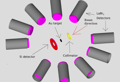
Figure 1: (Color online) The experimental setup is shown. Ten LaBr₃ detectors from the HAGRiD array are placed at ${30}^{\circ}$, ${60}^{\circ}$, ${90}^{\circ}$, ${120}^{\circ}$, and ${150}^{\circ}$ with respect to the beam axis surrounding the Au target, a brass collimator, and a S7 Si detector inside the scattering chamber (not shown).

The signals from the Si and LaBr₃ detectors were run through preamplifiers and into a digital data acquisition (DAQ) system using Pixie-16 modules from XIA, LLC [35]. In this experiment, a hit in any detector channel defined an event in the DAQ, with a hit in any another detector channel being considered coincident and packaged together into the same event if it occured within a ${500}\,{{\mathrm{ns}}}$ time window of the original event. In the second half of the experiment, this timing window was reduced to ${100}\,{{\mathrm{ns}}}$, to reduce the number of random coincidences in the $\gamma$-ray spectrum. The experiment was run for a total of 5 days with a beam rate of $4.1(3)\times 10^{5}$ pps. The precise determination of the beam rate is discussed in Section III.

At the end of the experiment, a ${1.44}\,{{\mathrm{\mu Ci}}}$ [152]Eu source was placed at the target location and the multiple $\gamma$ rays from its decay were used to calibrate each LaBr₃ detector in energy and determine its $\gamma$-ray efficiency. The entire array was found to have a total $\gamma$-ray efficiency of ${0.82}\,{\%}$ at ${1}\,{{\mathrm{MeV}}}$. The energy resolutions of the LaBr₃ detectors in the array were ${1.6}\,{-}$${2}\,{\%}$ at ${1408}\,{{\mathrm{keV}}}$. These resolutions were sufficient to cleanly resolve our $\gamma$-ray of interest (981 keV) since this energy is far enough away from the background $\gamma$-rays seen in the Doppler uncorrected spectrum.

III Analysis

To determine the $E2$ transition strength from our experimental observables, we needed to precisely determine our integrated beam rate over the course of the experiment and determine the $\gamma$-ray yield from the Coulomb-excited ⁸Li nuclei. The details of each step is outlined below.

In order to determine the total, integrated [8]Li beam current, we simulated the process of producing an in-flight beam with TwinSol, which leads to an extended spot size on the target. We modelled the beam as having a finite radius and offset from the center of the target. A fixed collimator upstream of the gold foils restricted the beam spot to a 9 mm radius, which was chosen to match the size of our gold target. Due to the proximity of the target to the Si detector, a diffuse beam will cause the [8]Li ions seen in the rings of the Si detector to come from a range of scattering angles. The Si detector also shows some up-down asymmetry in the measured rates in the sectors, indicating that the beam was offset to some degree. Because of the diffuse and asymmetric nature of the beam, comparing the distribution of the particles in the rings of the detector to a Rutherford distribution does not yield an accurate fit. We used a Geant4 [36, 37, 38] simulation to model the width and offset of the beam on target, accounting for the various scattering angles that result in counts in a single Si detector ring. The distribution of scattering angles seen in one of the inner rings of the Si detector is shown in Fig. 2.

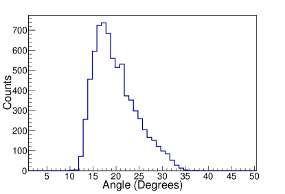
Figure 2: (Color online) A simulation of the distribution of angles of [8]Li particles observed in the first ring of the Si detector used in our analysis when using the beam spot determined by our simulation. The number of particles seen here is not representative of the total particles seen during the experiment, though the shape of the distribution should be accurate.

The radius of the beam and its offset from the beam axis were varied in the simulation over a range of values (1-7 mm for the radius and 1-4 mm for the offset) to reproduce the distribution seen in both the rings and sectors. We found a ${7}\,{{\mathrm{mm}}}$ beam radius and a ${1}\,{{\mathrm{mm}}}$ offset best reproduced the shape of the Si detector ring and sector data. The data seen in the Si rings and the simulation results are shown in Fig. 3. It can be seen that the simulation reproduces the shape of the measured counts in each Si detector ring very well. After the simulation reproduced the shape of the experimental data, it was scaled to have the same magnitude as the total number of counts measured during the experiment and a beam rate of $4.1(3)\times 10^{5}$ pps was extracted from the scaling. The beam rate uncertainty was estimated by changing the beam parameters and the beam scaling until the simulation results exceeded the experimental uncertainties.

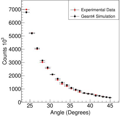
Figure 3: (Color online) A plot of [8]Li ions measured in the rings of the Si detector (circles) and the Geant4 simulated data (squares). The angles represent the center of each ring of the Si detector with the horizontal uncertainties showing the full angular extent of each ring.

A coincidence gate was placed on the scattered [8]Li peak seen in our Si detector in order to reduce the number of $\gamma$ rays from room background and the intrinsic radioactivity of the LaBr₃ detectors. As the Si ring and sector and LaBr₃ detector responsible for the coincidence event were known, the geometric angle between the scattered [8]Li particle and the emitted $\gamma$ ray was determined and used to correct for the Doppler shift of the $\gamma$-ray energy. During the analysis, a large amount of beam background was observed in the two innermost rings of the Si detector, which were therefore not included in this analysis.

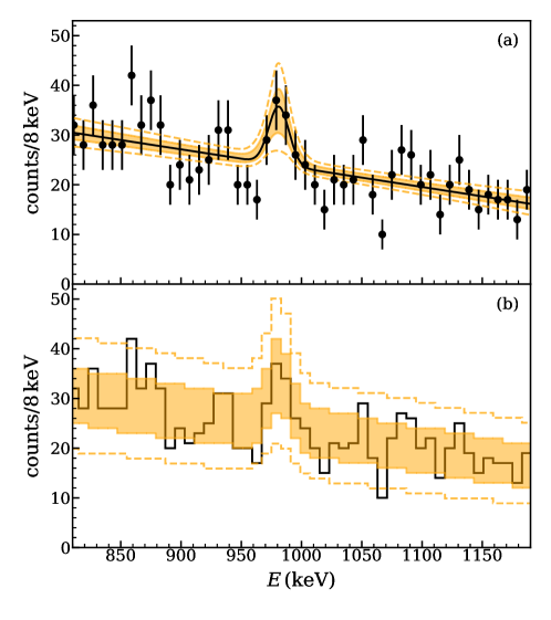
Figure 4: (Color online) The Doppler-corrected $\gamma$-ray spectrum summed over the entire experiment and in coincidence with the scattered-particle peak in the silicon detector. The spectrum is binned to 8 keV/bin. The $\gamma$-ray peak corresponding to the $2^{+}\rightarrow 1^{+}$ transition of [8]Li is seen at ${981}\,{{\mathrm{keV}}}$. In panel (a) the solid curve of the Gaussian function on a linear background with the most likely parameters is overlaid on the data, with the error bands representing 68% and 95% confidence intervals on the line of best fit. In panel (b) the uncertainty in the fit is folded with the Poisson statistical error and overlaid on the data; the spectrum is expected to lie within the band with 68% and 95% confidence.

Additionally, some of the random coincidences seen in the spectrum were eliminated by requiring a tight time coincidence between the LaBr and Si detector signals. The original coincidence window used in the experiment was 500 ns wide, but an additional timing gate was added in the offline analysis. The timing offsets between different rings of the Si detector and different LaBr₃ detectors were aligned and a 30 ns timing gate was placed over the position of the particle-$\gamma$ coincidences in the time difference spectrum. As the number of particle-$\gamma$ coincidences were low, this position was determined by observing the Doppler-corrected $\gamma$-ray spectrum while using a moving gate in the time-difference spectrum. The position and width were chosen to provide a robust $\gamma$-ray peak of interest at the expected peak position of ${980.8(1)}\,{{\mathrm{keV}}}$, the known literature value of the the $1^{+}\rightarrow 2^{+}$ transition [20]. The $\gamma$-ray spectrum in this energy range is shown in Fig. 4 and a small peak is visible above the background at the expected energy.

In order to determine the number of counts in the peak corresponding to the 981-keV $1^{+}\rightarrow 2^{+}$ transition in a robust way, we used Bayesian inference in modeling the spectrum with a Gaussian peak on a linear background:

$$n(E)=n_{0}+m(E-E_{0})+w\frac{A}{\sqrt{2\pi s^{2}}}e^{-(E-E_{0})^{2}/2s^{2}},$$ (1)

where $n_{0}$ and $m$ characterize the amplitude and energy slope of the background, $w$ is the width of the energy bins, and $A$, $s$, and $E_{0}$ characterize the area, width, and centroid energy of the peak, respectively. We calculated the posterior distribution of the fit parameters using a Markov-Chain Monte Carlo (MCMC) algorithm, implemented with the emcee package [39]. The likelihood function was obtained assuming that the probability for a datum in our spectrum is given by the Poisson distribution. Uniform priors were used for all parameters except the position and width of the peak. The uniform priors were properly normalized for a range of 0 to 75 for $n_{0}$, 0 to -1 for $m$, and 0 to 65 for the peak area $A$. For the peak position, a Gaussian prior with a $\sigma$ width corresponding to 1.5 keV was used. For the peak width $s$, the prior probability was given as $P(s)=\frac{\alpha^{\alpha-1}}{s_{0}^{2}\Gamma(\alpha-1)}e^{-\alpha\left(s_{0}/s\right)^{2}}\left(\frac{s_{0}}{s}\right)^{2\alpha}$, where $s_{0}=10\,\mathrm{keV}$ is the most likely or “expected” width of the peak, and the $\alpha=3$ specifies the shape of the distribution of possible widths. The value of $s_{0}=10\,\mathrm{keV}$ was chosen based on the measured widths of the LaBr₃ detectors’ intrinsic resolution from calibration data. Two-dimensional marginalized distributions of the calculated posterior probability density for all pairs of parameters and the marginalized distributions of one parameter are shown in Fig. 5.

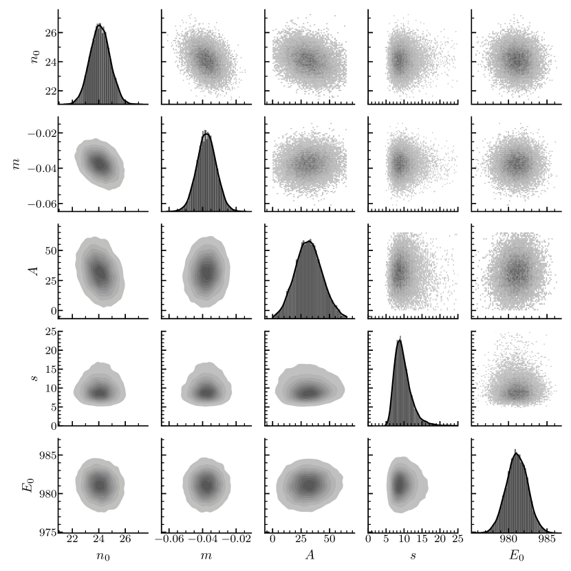
Figure 5: The marginalized distributions for the calculated posterior probability density function of the Gaussian and linear background parameters. The two-dimensional contour plots show the marginalized distribution for each pair of parameters and the one-dimensional histograms show the marginalized distributions for each parameter along the horizontal axis. The plots in the lower triangle are smoothed using kernel density estimation from the package seaborn [40], while the plots in the upper triangle are histograms of the Monte Carlo sample points. Similarly, the solid curves in the diagonal plots are smoothed using kernel density estimation, while the histograms represent the sample points.

The curve corresponding to the most likely parameters is plotted over the $\gamma$-ray spectrum in Fig. 4(a), along with 68% and 95% confidence intervals on the fit curve. In Fig. 4(b), we show the effect of including the Poisson statistics into the model prediction. From the posterior probability distribution for the model parameters (generated by the MCMC algorithm), we generate 15,000 synthetic $\gamma$-ray spectra; 68% of the generated spectra fall within the shaded band in Fig. 4(b), while 95% of the generated spectra fall between the dotted lines. The fact that the band in Fig. 4(b) is substantially wider than the band in Fig. 4(a) reflects the fact that, even for reasonably well-constrained fit parameters, we expect significant scatter in the spectrum entirely because of low counting statistics.

The most likely value of the area of the Gaussian peak is $31^{+13}_{-11}$ counts, where the error bar comes from the limits that correspond to 1$\sigma$ normal probabilities. For the other parameters, the maximum likelihood is given by $s=8.4^{+2.5}_{-1.7}$, $E_{0}=981.1(14)$, $m=0.038(6)$, and $n_{0}=24.1(7)$, again with 1$\sigma$ uncertainties. It is worth noting that the marginal distribution for the peak area is not Gaussian, especially for values approaching zero. Based on the area parameter’s marginal distribution, the interval corresponding to $2\sigma$ (97.7% probability) excludes a lower value below 9.0 counts. The implication of these peak area values on the deduced $B(E2)$ values will be discussed later in this section.

In addition to looking at the posterior distributions, we have also analyzed the $\gamma$-ray spectrum using a Bayes factor analysis. The Bayes factor is a ratio of posterior probabilities for two hypotheses and can be used in model selection [41]. One of these hypotheses can be the null hypothesis and the one we have chosen is that there is no peak that exists at 981 keV. In this hypothesis, the spectrum is described only by a linear background. The Bayes factor disfavors the use of many adjustable parameters so a hypothesis with a smaller number of parameters that can describe the data equally well will be favored over one with a larger number of parameters. This means that model selection using the Bayes factor is not solely based on how well the data is fit by the model but will favor the simpler model in the case that both models fit the data equally well. One of the most important inputs into the Bayes factor is the prior probability for the peak area. As mentioned previously, we have chosen a uniform prior for the area with a range of 0 to 65 counts, a reasonable and generous assumption. In order to calculate the Bayes factor, we use a sequential Monte Carlo (SMC) algorithm, as implemented by the PyMC3 package [42]. We obtain a Bayes factor of 9.0 when comparing the “peak” hypothesis to the null hypothesis. This value falls squarely in the range given by Ref. [41] of 3 to 20, which is considered “positive” evidence against the null hypothesis. Although this value of the Bayes factor does not completely exclude the null hypothesis, there is substantial evidence for the “peak” hypothesis such that it should not be ruled out.

Using the measured efficiency of the LaBr₃ array and the most likely value for the number of counts observed in the 981 keV $\gamma$-ray peak, we were able to determine the absolute $\gamma$-ray yield for the experiment.

The final step was to determine the [8]Li $B(E2;2^{+}\rightarrow 1^{+})$ value from the total $\gamma$-ray yield in the experiment. We used a version of the Winther-De Boer Coulomb excitation code, which is based on the semi-classical theory of Coulomb excitation [43]. This version of the code was capable of calculating electric dipole to hexadecapole transitions and also multiple excitations. After inputting an ${E}2$ matrix element, the code outputs a differential cross section which can be used to match the output of the $\gamma$-ray yield measured in the experiment. Due to the shape of the [8]Li beam, varying scattering angles in each Si detector ring, and Si detector geometric efficiencies, it would be difficult to account for in a simple calculation. Therefore, we used the Geant4 simulation to use the event-by-event simulated angle to determine the proper Coulomb-excitation probability given by the Winther-De Boer calculations. We determine the $B(E2)$ by finding the value that matches our experimental $\gamma$-ray yield through the Geant4 simulation. The [8]Li $B(E2;2^{+}\rightarrow 1^{+})$ value we obtained is ${19^{+7}_{-6}}\,{e^{2}{\mathrm{fm}}^{4}}$, which includes the $\gamma$-ray yield statistical and beam rate uncertainties.

Coming back to the values of the peak area that are excluded by a $2\sigma$ interval, the $B(E2;2^{+}\rightarrow 1^{+})$ value less than ${5.2}\,{e^{2}{\mathrm{fm}}^{4}}$ are excluded with a 97.7% probability based on our data. This probability does not favor theoretical predictions, which will be discussed in detail in Sec. IV.

The two sources of systematic uncertainties are the $M1$ component of the excitation probability and contributions from electric dipole polarizability, i.e., virtual $E1$ excitations to collective structures at high energy. Based on a study of [7]Li [44], which should be a fairly close analogue to [8]Li, we estimate the $M1$ contribution at the forward angles in our experiment to be between 2-3%. Much less easily understood is the effect of the $E1$ dipole polarizability. Unlike [7]Li, which has a strong virtual excitation to the break up of [3]H+$\alpha$, [8]Li mainly virtually excites to levels that decay by neutron emission. Studies on the $E1$ dipole polarization effect in ⁶Li and ⁷Li suggest that this effect is small, on the order of less than 10% at forward angles [44, 45]. With a conservative estimate of 3$\%$ uncertainty due to the M1 excitation and a 10$\%$ uncertainty due to the effect of $E1$ dipole polarizability, we account for these by assigning a systematic uncertainty in the $\gamma$-ray peak area, which results in an uncertainty in the $B(E2)$ of 2 e²fm⁴. More precise measurements in the future that approach 10% precision will need to more carefully consider and estimate the strength of the virtual $E1$ breakup. In addition, a calculation was performed using a coupled-channel code to estimate the effect of $E2$ excitations to the unbound 3${}^{+}_{1}$ level, the level closest to the neutron threshold. It was found that the cross section for this excitation was a factor of 1000 less likely than to the first excited 1⁺ level. It is therefore unlikely then that two-step processes to known levels would significantly contribute to our deduced $B(E2)$ value.

Last, a possible mechanism for the population of the first 1⁺ state in ⁸Li is the excitation from the non-resonant continuum in the Coulomb excitation process. The possible magnitude of this contribution is currently unknown. A future reaction theory calculation using, for example, the Extended Continuum Discretized Coupled Channels method [46, 47, 48], would be able to estimate such a contribution.

IV Discussion

Table 1: Experimental ground-state $E2$ moments [26], for $\isotope[8]{Li}$ and selected neighboring nuclides, and transition strengths to the first excited rotational band member [1, 2, 17], where available. The rotational intrinsic quadrupole moment extracted from the experimental ground state quadrupole moment is given, along with the corresponding expected rotational $E2$ strength.

	Experiment				Rotational
Nuclide	$J^{P}_{\text{gs}}$	$Q$ (${\mathrm{fm}}^{2}$)	$J^{P}_{\text{ex}}$	$B(E2\uparrow)$ ($e^{2}{\mathrm{fm}}^{4}$)	$K$	$Q_{0}$ (${\mathrm{fm}}^{2}$)	$B(E2\uparrow)$ ($e^{2}{\mathrm{fm}}^{4}$)
$\isotope[7]{Li}$	$3/2^{-}$	$-4.00(3)$	$1/2^{-}$	$8.3(5)$	$1/2$	$\approx+20$	$\approx 8.0$
$\isotope[7]{Be}$	$3/2^{-}$	$\approx-6.8$	$1/2^{-}$	$26(6)(3)$	$1/2$	$\approx+34$	$\approx 23$
$\isotope[8]{Li}$	$2^{+}$	$+3.14(2)$	$3^{+}$	—	$2$	$\approx+11$	$\approx 6.0$
			$1+$	$19^{+7}_{-6}(2)$	$2\rightarrow 1$		$\lesssim 2$
$\isotope[8]{B}$	$2^{+}$	$+6.34(14)$	$3^{+}$	—	$2$	$\approx+22$	$\approx 25$
$\isotope[9]{Be}$	$3/2^{-}$	$+5.29(4)$	$5/2^{-}$	$42(3)$	$3/2$	$\approx+27$	$\approx 36$

Estimated from mirror nuclide quadrupole moment via ab initio calculations [49].
Indicated experimental uncertainties, from Ref. [17], are statistical and systematic, respectively.
Present work.

The present measured $B(E2;2^{+}\rightarrow 1^{+})=19^{+7}_{-6}(2)\,e^{2}{\mathrm{fm}}^{4}$ in $\isotope[8]{Li}$, while still enhanced relative to the Weisskopf single-particle strength ($\approx 0.95\,e^{2}{\mathrm{fm}}^{4}$ for $A=8$), is reduced relative to the prior reported $55(15)\,e^{2}{\mathrm{fm}}^{4}$ [18]. The present value is now well within the range of $E2$ strengths observed in neighboring $A=7$ and $9$ nuclides, which reach $\approx 42\,e^{2}{\mathrm{fm}}^{4}$ in $\isotope[9]{Be}$.

Nonetheless, the measured strength is still difficult to accommodate within structural understanding of this nuclide. The enhanced $E2$ strengths in neighboring nuclides are readily understood in terms of collective rotational enhancement, which cannot so simply explain an enhanced $2^{+}\rightarrow 1^{+}$ strength in $\isotope[8]{Li}$ [50]. Even assuming the $2^{+}$ ground state to be the band head of a $K=2$ rotational band, there would be no $1^{+}$ band member. Ab initio theory, while successfully reproducing enhanced rotational transitions in neighboring nuclides, does not predict enhancement of the $2^{+}\rightarrow 1^{+}$ strength in $\isotope[8]{Li}$ [50].

The deformation and the corresponding $E2$ enhancement in $\isotope[8]{Li}$ and its neighbors is understood to arise from cluster structure [6, *vonoertzen1997:be-alpha-rotational, 8, 9]. In a cluster molecular picture for these nuclei, these nuclei are cluster dimers, with possible additional nucleons occupying molecular orbitals around this dimer core. Thus, $\isotope[7]{Li}$ may be viewed as $\alpha+t$, $\isotope[8]{Be}$ as $\alpha+\alpha$, $\isotope[9]{Be}$ as $\alpha+\alpha+n$, etc. It is thus reasonable to expect axially-symmetric rotation. In a rotational strong coupling picture [27, 28], any additional nucleons are taken to be coupled to the axially-symmetric rotational core.

Directly comparing the different $E2$ strengths in $\isotope[8]{Li}$ and its neighbors is meaningless without taking into account the geometric factors arising from rotational motion. Recall that axially-symmetric rotation gives rise to simple relations among all $E2$ matrix elements within a band [51, 27, 28, 52, *maris2019:berotor2-ERRATUM]. In particular, all states within a rotational band share the same rotational intrinsic state $|\phi_{K}\rangle$ in the body-fixed frame, and the spectroscopic quadrupole moments $Q(J)$ and reduced transition probabilities $B(E2;J_{i}\rightarrow J_{f})$ are all obtained in terms of a single intrinsic $E2$ matrix element, or intrinsic quadrupole moment $Q_{0}$. The rotational $E2$ strengths are thus tied to the ground state quadrupole moments, which are precisely-measured for many of these nuclei [26].

In $\isotope[7]{Li}$, the close-lying $3/2^{-}$ ground state and $1/2^{-}$ excited state are interpreted as members of a $K=1/2$ rotational band, where the energy order is inverted due to Coriolis staggering [28] (see, e.g., Fig. 3 of Ref. [54]). For $\isotope[7]{Li}$ the measured $Q(3/2^{-})=-4.00(3)\,{\mathrm{fm}}^{2}$ [26] yields an intrinsic quadrupole moment of $Q_{0}\approx+20\,{\mathrm{fm}}^{2}$, and thus a rotational prediction $B(E2;3/2^{-}\rightarrow 1/2^{-})\approx 8.0\,e^{2}{\mathrm{fm}}^{4}$, consistent with the experimental $8.3(5)\,e^{2}{\mathrm{fm}}^{4}$ [1]. (This and subsequent rotational comparisons are summarized in Table IV.)

For $\isotope[7]{Be}$, the ground state quadrupole moment is not experimentally known. However, in a cluster picture, $\isotope[7]{Be}$ is obtained from $\isotope[7]{Li}$ by replacing the triton ($\isotope[3]{H}$) cluster with a $\isotope[3]{He}$ cluster. In the limit of well-separated point clusters, i.e., a “ball-and-stick model”, this substitution gives $Q(\isotope[7]{Be})/Q(\isotope[7]{Li})=50/34\approx 1.5$ [49], yielding $Q_{0}\approx+29\,{\mathrm{fm}}^{2}$, while ab initio predictions give a somewhat larger ratio of $\approx 1.7$ [15, 49], yielding $Q_{0}\approx+34\,{\mathrm{fm}}^{2}$. Thus, in a rotational picture, we expect $B(E2;3/2^{-}\rightarrow 1/2^{-})\approx 23\,e^{2}{\mathrm{fm}}^{4}$ for $\isotope[7]{Be}$, again consistent with the experimental value $26(6)(3)\,e^{2}{\mathrm{fm}}^{4}$ [17].

In the heavier neighbor $\isotope[9]{Be}$, the $3/2^{-}$ ground state is understood to be the band head of a $K=3/2$ rotational band, with the $5/2^{-}$ excited state as a band member (see, e.g., Fig. 1 of Ref. [54]). The measured $Q(3/2^{-})=+5.29(4)\,{\mathrm{fm}}^{2}$ [26] yields an intrinsic quadrupole moment of $Q_{0}\approx+27\,{\mathrm{fm}}^{2}$, and thus a rotational prediction $B(E2;3/2^{-}\rightarrow 5/2^{-})\approx 36\,e^{2}{\mathrm{fm}}^{4}$, on the same order as the experimental $42(3)\,e^{2}{\mathrm{fm}}^{4}$ [2], albeit not to within experimental uncertainties.

The ground state of $\isotope[8]{B}$, mirror nuclide to $\isotope[8]{Li}$, has been interpreted as consisting of a proton coupled to a deformed $\isotope[7]{Be}$ core. A spatially-extended molecular orbital for the proton has been proposed (from fermionic molecular dynamics calculations) to lead to proton halo structure [25] and also suggested to contribute to the enhanced ground-state quadrupole moment [21, 55]. Assuming the ground state to be a $K=2$ band head, the measured $Q(2^{+})=+6.34(14)\,{\mathrm{fm}}^{2}$ [26] yields an intrinsic quadrupole moment of $Q_{0}\approx+22\,{\mathrm{fm}}^{2}$ (Table IV).

However, returning to $\isotope[8]{Li}$, the measured $Q(2^{+})=+3.14(2)\,{\mathrm{fm}}^{2}$ [26], at about half that of $\isotope[8]{B}$, yields an intrinsic quadrupole moment of only $Q_{0}\approx+11\,{\mathrm{fm}}^{2}$, the lowest among the nuclides discussed thus far by nearly a factor of $2$ (Table IV), making any $E2$ enhancement harder to explain. Such a lower intrinsic quadrupole moment, relative to the mirror nuclide $\isotope[8]{B}$, is reasonable in light of the lower quadrupole moment of the $\isotope[7]{Li}$ core and the replacement of the charged halo proton by an uncharged halo neutron.

For the $2^{+}\rightarrow 1^{+}$ transition, the $1^{+}$ first excited state in $\isotope[8]{Li}$ cannot be a member of the $K=2$ ground state band. Even if this $1^{+}$ state is rotational in nature, it must rather be a band head in its own right — of either a $K=1$ band or, conceivably, a $K=0$ band with negative signature (and thus $J=1,3,\dots$ [27, 28]). The transition to this state is then interband transition, requiring a change in the rotational intrinsic wave function.

In the cluster molecular orbital description, we may expect the valence neutron to be in a $\pi$ orbital with $K=3/2$, as in the isotone $\isotope[9]{Be}$ [56]. The $K$ quantum number adds algebraically, so the $K=2$ ground state band is obtained from aligned coupling of this neutron with the $K=1/2$ $\isotope[7]{Li}$ core, while the $1^{+}$ excited state is ostensibly the band head of a $K=1$ band arising from the antialigned coupling.

Even if, as a generous upper limit, we were to take the interband intrinsic matrix element $\langle{\phi_{K=1}}|{Q_{2,-1}}|{\phi_{K=2}}\rangle$ to be identical in size to the diagonal intrinsic matrix element $\langle{\phi_{K=2}}|{Q_{2,0}}|{\phi_{K=2}}\rangle$ determining the ground state band’s intrinsic quadrupole moment, the rotational picture would give $B(E2;2^{+}\rightarrow 1^{+})/[eQ(2^{+})]^{2}\lesssim 0.24$, or $B(E2;2^{+}\rightarrow 1^{+})\lesssim 2\,e^{2}{\mathrm{fm}}^{4}$. Only under the less-motivated assumption that the $1^{+}$ excited state is the band head of a negative-signature $K=0$ band does a transition on the scale of the present measurement become plausible. Taking the interband intrinsic matrix element, now $\langle{\phi_{K=0}}|{Q_{2,-2}}|{\phi_{K=2}}\rangle$, to again be of the same size as the diagonal intrinsic matrix element gives $B(E2;2^{+}\rightarrow 1^{+})/[eQ(2^{+})]^{2}\lesssim 0.98$, or $B(E2;2^{+}\rightarrow 1^{+})\lesssim 10\,e^{2}{\mathrm{fm}}^{4}$, but is the less favored scenario.

V Summary

We have performed a radioactive-beam Coulomb excitation experiment to remeasure the $2^{+}\rightarrow 1^{+}$ $E2$ strength in $\isotope[8]{Li}$, now making use of particle-$\gamma$ coincidences. Compared to the previously-reported $B(E2;2^{+}\rightarrow 1^{+})=55(14)\,e^{2}{\mathrm{fm}}^{4}$ [18], our measured value of $19^{+7}_{-6}(2)\,e^{2}{\mathrm{fm}}^{4}$ is smaller by approximately a factor of three, but remains difficult to accommodate within a theoretical understanding of the nuclear structure.

The enhanced $E2$ strengths in the neighboring $A=7$ and $9$ nuclei are naturally understood in terms of in-band rotational transitions, and we find that they are well-described by ab initio predictions. However, there is no simple way to explain an enhanced $2^{+}\rightarrow 1^{+}$ transition in $\isotope[8]{Li}$. Such a transition is not naturally viewed as a rotational in-band transition, and it is unnaturally large for an interband transition.

The magnitude of possible contributions from the non-resonant continuum to the cross section, and thus to the $E2$ strength extracted from experiment, is unknown. Calculations from reaction theory to estimate such contributions from the continuum could clarify if they might explain the discrepancy between experiment and theory. Other possible contributions to the cross section, from two-step Coulomb excitation (or dipole polarization), involving virtual excitation of higher-lying states above the neutron separation threshold, as well as from indirect feeding involving direct excitation of these states, are estimated to be insufficient to explain the discrepancy. The use of particle-$\gamma$ coincidences in the present experiment eliminates any significant contribution from $\isotope[8]{Li}$ $1^{+}\rightarrow 2^{+}$ $\gamma$ rays that are produced in the primary reaction, removing a possible experimental inflation of the $B(E2)$ value. In conclusion, our studies confirm that there is no easy interpretation for a large $B(E2)$ in $\isotope[8]{Li}$, and our experimental result reinforces the tension between experiment and theory suggested by the previous work.

Acknowledgments

We thank Colin V. Coane, Jakub Herko, and Zhou Zhou for comments on the manuscript and Filomena Nuñes for discussions on contributions from the non-resonant continuum. This work was supported by the U.S. National Science Foundation under Grant Nos. PHY 20-11890, PHY 17-13857, PHY 14-01343, and PHY 14-30152, and by the U.S. Department of Energy, Office of Science, under Award Nos. DE-FG02-95ER40934, DE-SC021027, and FRIB Theory Alliance award DE-SC0013617 and sponsored in part by the National Nuclear Security Administration under the Stewardship Science Academic Alliance program through DOE Cooperative Agreement No. DE-NA000213. This research used computational resources of the University of Notre Dame Center for Research Computing and of the National Energy Research Scientific Computing Center (NERSC), a U.S. Department of Energy, Office of Science, user facility supported under Contract DE-AC02-05CH11231. Figures in this work were produced using ROOT [57], matplotlib [58], and seaborn [40].

References

- Tilley et al. [2002] D. R. Tilley, C. M. Cheves, J. L. Godwin, G. M. Hale, H. M. Hofmann, J. H. Kelley, C. G. Sheu, and H. R. Weller, Nucl. Phys. A 708, 3 (2002).
- Tilley et al. [2004] D. R. Tilley, J. H. Kelley, J. L. Godwin, D. J. Millener, J. E. Purcell, C. G. Sheu, and H. R. Weller, Nucl. Phys. A 745, 155 (2004).
- Inglis [1953] D. R. Inglis, Rev. Mod. Phys. 25, 390 (1953).
- Millener [2001] D. J. Millener, Nucl. Phys. A 693, 394 (2001).
- Datar et al. [2013] V. M. Datar, D. R. Chakrabarty, S. Kumar, V. Nanal, S. Pastore, R. B. Wiringa, S. P. Behera, A. Chatterjee, D. Jenkins, C. J. Lister, E. T. Mirgule, A. Mitra, R. G. Pillay, K. Ramachandran, O. J. Roberts, P. C. Rout, A. Shrivastava, and P. Sugathan, Phys. Rev. Lett. 111, 062502 (2013).
- von Oertzen [1996] W. von Oertzen, Z. Phys. A 354, 37 (1996).
- von Oertzen [1997] W. von Oertzen, Z. Phys. A 357, 355 (1997).
- Freer [2007] M. Freer, Rep. Prog. Phys. 70, 2149 (2007).
- Kanada-En’yo et al. [2012] Y. Kanada-En’yo, M. Kimura, and A. Ono, Prog. Exp. Theor. Phys. 2012, 01A202 (2012).
- Maris [2012] P. Maris, J. Phys. Conf. Ser. 402, 012031 (2012).
- Kravvaris and Volya [2017] K. Kravvaris and A. Volya, Phys. Rev. Lett. 119, 062501 (2017).
- Casten [2000] R. F. Casten, Nuclear Structure from a Simple Perspective, 2nd ed., Oxford Studies in Nuclear Physics No. 23 (Oxford University Press, Oxford, 2000).
- Wiringa et al. [2000] R. B. Wiringa, S. C. Pieper, J. Carlson, and V. R. Pandharipande, Phys. Rev. C 62, 014001 (2000).
- Pervin et al. [2007] M. Pervin, S. C. Pieper, and R. B. Wiringa, Phys. Rev. C 76, 064319 (2007).
- Pastore et al. [2013] S. Pastore, S. C. Pieper, R. Schiavilla, and R. B. Wiringa, Phys. Rev. C 87, 035503 (2013).
- Pastore et al. [2014] S. Pastore, R. B. Wiringa, S. C. Pieper, and R. Schiavilla, Phys. Rev. C 90, 024321 (2014).
- Henderson et al. [2019] S. L. Henderson, T. Ahn, M. A. Caprio, P. J. Fasano, A. Simon, W. Tan, P. O’Malley, J. Allen, D. W. Bardayan, D. Blankstein, B. Frentz, M. R. Hall, J. J. Kolata, A. E. McCoy, S. Moylan, C. S. Reingold, S. Y. Strauss, and R. O. Torres-Isea, Phys. Rev. C 99, 064320 (2019).
- Brown et al. [1991] J. A. Brown, F. D. Becchetti, J. W. Jänecke, K. Ashktorab, D. A. Roberts, J. J. Kolata, R. J. Smith, K. Lamkin, and R. E. Warner, Phys. Rev. Lett. 66, 2452 (1991).
- Throop et al. [1971] M. J. Throop, D. H. Youngblood, and G. C. Morrison, Phys. Rev. C 3, 536 (1971).
- Costa et al. [1972] G. Costa, F. Beck, and D. Magnac-Valette, Nuclear Physics A 181, 174 (1972).
- Minamisono et al. [1992] T. Minamisono, T. Ohtsubo, I. Minami, S. Fukuda, A. Kitagawa, M. Fukuda, K. Matsuta, Y. Nojiri, S. Takeda, H. Sagawa, and H. Kitagawa, Phys. Rev. Lett. 69, 2058 (1992).
- Smedberg et al. [1999] M. H. Smedberg, T. Baumann, T. Aumann, L. Axelsson, U. Bergmann, M. J. G. Borge, D. Cortina-Gil, L. M. Fraile, H. Geissel, L. Grigorenko, M. Hellström, M. Ivanov, N. Iwasa, R. Janik, B. Jonson, H. Lenske, K. Markenroth, G. Münzenberg, T. Nilsson, A. Richter, K. Riisager, C. Scheidenberger, G. Schrieder, W. Schwab, H. Simon, B. Sitar, P. Strmen, K. Sümmerer, M. Winkler, and M. V. Zhukov, Phys. Lett. B 452, 1 (1999).
- Jonson [2004] B. Jonson, Phys. Rep. 389, 1 (2004).
- Korolev et al. [2018] G. A. Korolev, A. V. Dobrovolsky, A. G. Inglessi, G. D. Alkhazov, P. Egelhof, A. Estradé, I. Dillmann, F. Farinon, H. Geissel, S. Ilieva, Y. Ke, A. V. Khanzadeev, O. A. Kiselev, J. Kurcewicz, X. C. Le, Y. A. Litvinov, G. E. Petrov, A. Prochazka, C. Scheidenberger, L. O. Sergeev, H. Simon, M. Takechi, S. Tang, V. Volkov, A. A. Vorobyov, H. Weick, and V. I. Yatsoura, Phys. Lett. B 780, 200 (2018).
- Henninger et al. [2015] K. R. Henninger, T. Neff, and H. Feldmeier, J. Phys. Conf. Ser. 599, 012038 (2015).
- Stone [2016] N. J. Stone, At. Data Nucl. Data Tables 111, 1 (2016).
- Bohr and Mottelson [1998] A. Bohr and B. R. Mottelson, Nuclear Structure, Vol. 1 (World Scientific, Singapore, 1998).
- Rowe [2010] D. J. Rowe, Nuclear Collective Motion: Models and Theory (World Scientific, Singapore, 2010).
- Barrett et al. [2013] B. R. Barrett, P. Navrátil, and J. P. Vary, Prog. Part. Nucl. Phys. 69, 131 (2013).
- Calci and Roth [2016] A. Calci and R. Roth, Phys. Rev. C 94, 014322 (2016).
- Becchetti et al. [2003] F. D. Becchetti, M. Y. Lee, T. W. O’Donnell, D. A. Roberts, J. J. Kolata, L. O. Lamm, G. Rogachev, V. Guimarães, P. A. DeYoung, and S. Vincent, Nuclear Instruments and Methods in Physics Research A 505, 377 (2003).
- Henderson [2021] S. L. Henderson, Studies of nuclear structure by measurements in and , Ph.D. thesis, University of Notre Dame (2021).
- [33] Micron Semiconductor Ltd, http://www.micronsemiconductor.co.uk, accessed: 2022-03-11.
- Smith et al. [2018] K. Smith, T. Baugher, S. Burcher, A. Carter, J. Cizewski, K. Chipps, M. Febbraro, R. Grzywacz, K. Jones, S. Munoz, S. Pain, S. Paulauskas, A. Ratkiewicz, K. Schmitt, C. Thornsberry, R. Toomey, D. Walter, and H. Willoughby, Nuclear Instruments and Methods in Physics Research Section B: Beam Interactions with Materials and Atoms 414, 190 (2018).
- [35] XIA LLC, https://xia.com, accessed: 2022-03-11.
- TODO FIX GARBAGE CHARACTERS [2003] TODO FIX GARBAGE CHARACTERS, Nuclear Instruments and Methods in Physics Research Section A: Accelerators, Spectrometers, Detectors and Associated Equipment 506, 250 (2003).
- Allison et al. [2006] J. Allison, K. Amako, J. Apostolakis, H. Araujo, P. A. Dubois, M. Asai, G. Barrand, R. Capra, S. Chauvie, R. Chytracek, G. A. P. Cirrone, G. Cooperman, G. Cosmo, G. Cuttone, G. G. Daquino, M. Donszelmann, M. Dressel, G. Folger, F. Foppiano, J. Generowicz, V. Grichine, S. Guatelli, P. Gumplinger, A. Heikkinen, I. Hrivnacova, A. Howard, S. Incerti, V. Ivanchenko, T. Johnson, F. Jones, T. Koi, R. Kokoulin, M. Kossov, H. Kurashige, V. Lara, S. Larsson, F. Lei, O. Link, F. Longo, M. Maire, A. Mantero, B. Mascialino, I. McLaren, P. M. Lorenzo, K. Minamimoto, K. Murakami, P. Nieminen, L. Pandola, S. Parlati, L. Peralta, J. Perl, A. Pfeiffer, M. G. Pia, A. Ribon, P. Rodrigues, G. Russo, S. Sadilov, G. Santin, T. Sasaki, D. Smith, N. Starkov, S. Tanaka, E. Tcherniaev, B. Tome, A. Trindade, P. Truscott, L. Urban, M. Verderi, A. Walkden, J. P. Wellisch, D. C. Williams, D. Wright, and H. Yoshida, IEEE Trans. Nucl. Sci. 53, 270 (2006).
- Allison et al. [2016] J. Allison, K. Amako, J. Apostolakis, P. Arce, M. Asai, T. Aso, E. Bagli, A. Bagulya, S. Banerjee, G. Barrand, B. Beck, A. Bogdanov, D. Brandt, J. Brown, H. Burkhardt, P. Canal, D. Cano-Ott, S. Chauvie, K. Cho, G. Cirrone, G. Cooperman, M. Cortés-Giraldo, G. Cosmo, G. Cuttone, G. Depaola, L. Desorgher, X. Dong, A. Dotti, V. Elvira, G. Folger, Z. Francis, A. Galoyan, L. Garnier, M. Gayer, K. Genser, V. Grichine, S. Guatelli, P. Guèye, P. Gumplinger, A. Howard, I. Hřivnáčová, S. Hwang, S. Incerti, A. Ivanchenko, V. Ivanchenko, F. Jones, S. Jun, P. Kaitaniemi, N. Karakatsanis, M. Karamitros, M. Kelsey, A. Kimura, T. Koi, H. Kurashige, A. Lechner, S. Lee, F. Longo, M. Maire, D. Mancusi, A. Mantero, E. Mendoza, B. Morgan, K. Murakami, T. Nikitina, L. Pandola, P. Paprocki, J. Perl, I. Petrović, M. Pia, W. Pokorski, J. Quesada, M. Raine, M. Reis, A. Ribon, A. R. Fira, F. Romano, G. Russo, G. Santin, T. Sasaki, D. Sawkey, J. Shin, I. Strakovsky, A. Taborda, S. Tanaka, B. Tomé, T. Toshito, H. Tran, P. Truscott, L. Urban, V. Uzhinsky, J. Verbeke, M. Verderi, B. Wendt, H. Wenzel, D. Wright, D. Wright, T. Yamashita, J. Yarba, and H. Yoshida, Nucl. Instrum. Meth. A 835, 186 (2016).
- Foreman-Mackey et al. [2013] D. Foreman-Mackey, D. W. Hogg, D. Lang, and J. Goodman, Publ. Astron. Soc. Pac. 125, 306 (2013), arXiv:1202.3665 [astro-ph.IM] .
- Waskom [2021] M. L. Waskom, J. Open Source Softw. 6, 3021 (2021).
- Kass and Raftery [1995] R. E. Kass and A. E. Raftery, Journal of the American Statistical Association 90, 773 (1995).
- Salvatier et al. [2016] J. Salvatier, T. V. Wiecki, and C. Fonnesbeck, Peer J Computer Science 2, e55 (2016).
- Alder et al. [1956] K. Alder, A. Bohr, T. Huus, B. Mottelson, and A. Winther, Reviews of Modern Physics 28, 432 (1956).
- Häusser et al. [1973] O. Häusser, A. McDonald, T. Alexander, A. Ferguson, and R. Warner, Nuclear Physics A 212, 613 (1973).
- Disdier et al. [1971] D. L. Disdier, G. C. Ball, O. Häusser, and R. E. Warner, Physical Review Letters 27, 1391 (1971).
- Nunes et al. [1996] F. Nunes, I. Thompson, and R. Johnson, Nuclear Physics A 596, 171 (1996).
- Summers et al. [2006] N. C. Summers, F. M. Nunes, and I. J. Thompson, Phys. Rev. C 74, 014606 (2006).
- Summers et al. [2014] N. C. Summers, F. M. Nunes, and I. J. Thompson, Phys. Rev. C 89, 069901 (2014).
- Caprio et al. [2021] M. A. Caprio, P. J. Fasano, P. Maris, and A. E. McCoy, Phys. Rev. C 104, 034319 (2021).
- Caprio and Fasano [2022] M. A. Caprio and P. J. Fasano, Phys. Rev. C 106, 034320 (2022).
- Alaga et al. [1955] G. Alaga, K. Alder, A. Bohr, and B. R. Mottelson, Mat. Fys. Medd. Dan. Vid. Selsk. 29 (1955).
- Maris et al. [2015] P. Maris, M. A. Caprio, and J. P. Vary, Phys. Rev. C 91, 014310 (2015).
- Maris et al. [2019] P. Maris, M. A. Caprio, and J. P. Vary, Phys. Rev. C 99, 029902(E) (2019).
- Caprio et al. [2020] M. A. Caprio, P. J. Fasano, P. Maris, A. E. McCoy, and J. P. Vary, Eur. Phys. J. A 56, 120 (2020).
- Kitagawa and Sagawa [1993] H. Kitagawa and H. Sagawa, Phys. Lett. B 299, 1 (1993).
- Della Rocca and Iachello [2018] V. Della Rocca and F. Iachello, Nucl. Phys. A 973, 1 (2018).
- Brun and Rademakers [1997] R. Brun and F. Rademakers, Nuclear Instruments and Methods in Physics Research Section A: Accelerators, Spectrometers, Detectors and Associated Equipment 389, 81 (1997), new Computing Techniques in Physics Research V.
- Hunter [2007] J. D. Hunter, Comput. Sci. Eng. 9, 90 (2007).