mmdshort = MMD, long = maximum mean discrepancy rkhsshort = RKHS, long = reproducing kernel Hilbert space qmcshort = QMC, long = quasi Monte Carlo pdfshort = PDF, long = probability density function ksdshort = KSD, long = kernel Stein discrepancy mcmcshort = MCMC, long = Markov chain Monte Carlo smcshort = SMC, long = sequential Monte Carlo

Minimum Discrepancy Methods in Uncertainty Quantification

These lectures concern the discrete approximation of objects that are in some sense infinite-dimensional. This problem is ubiquitous to numerical computation in general. Specifically, we will consider discrete approximation of probability distributions $P$ that may be defined on an infinite set, such as $[0,1]^{d}$ or $\mathbb{R}^{d}$. See Figure 1. The basic questions here are: (1) how many states are required to achieve a given level of approximation? (2) how can such approximations be constructed?

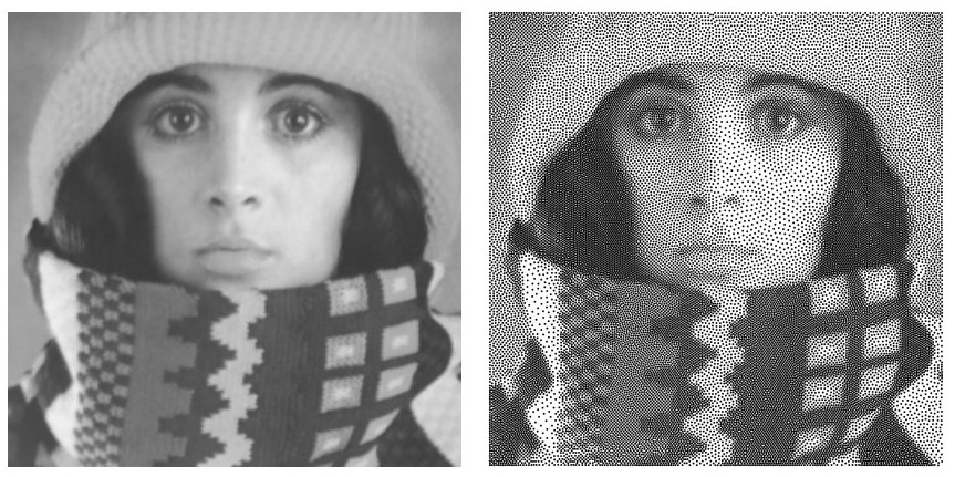
Figure 1: Quantisation is the act of approximating a probability distribution $P$, defined on an infinite set, with a discrete distribution $\sum_{i=1}^{n}w_{i}\delta(\bm{x}_{i})$ supported on a finite set of states $\{\bm{x}_{i}\}_{i=1}^{n}$. Here $\delta(\bm{x}_{i})$ denotes a Dirac distribution centred at $\bm{x}_{i}$. The left image can be considered to represent a pdf $p(\bm{x})$ for $P$, defined for $\bm{x}\in[0,1]^{d}$, and the dots in the right image can be considered to represent $\bm{x}_{i}$, with the size of the does representing $w_{i}$. This image is due to Gräf et al. (2012).

1 Classical Discrepancy Theory

Here we start with some motivation from a classical perspective, which considers approximation of the uniform distribution $P$ on $[0,1]^{d}$ by an (un-weighted) collection of states $\{\bm{x}_{i}\}_{i=1}^{n}$. For $\bm{x}\in[0,1]^{d}$, let $[\bm{0},\bm{x})=[0,x_{1})\times\dots\times[0,x_{d})$.

Definition 1 (Local discrepancy).

The local discrepancy of a collection of states $\bm{x}_{1},\dots,\bm{x}_{n}\in[0,1]^{d}$ at $\bm{a}\in[0,1]^{d}$ is

$$\Delta(\bm{a})=\Delta(\bm{a};\bm{x}_{1},\dots,\bm{x}_{n})=\frac{1}{n}\sum_{i=1}^{n}\mathbbm{1}_{[\bm{0},\bm{a})}(\bm{x}_{i})-\prod_{j=1}^{d}a_{j}.$$

Definition 2 (Star discrepancy).

The star discrepancy of $\bm{x}_{1},\dots,\bm{x}_{n}\in[0,1]^{d}$ is

$$D_{n}^{*}=D_{n}^{*}(\bm{x}_{1},\dots,\bm{x}_{n})=\sup_{\bm{a}\in[0,1)^{d}}|\Delta(\bm{a};\bm{x}_{1},\dots,\bm{x}_{n})|.$$

See the illustration in Figure 2.

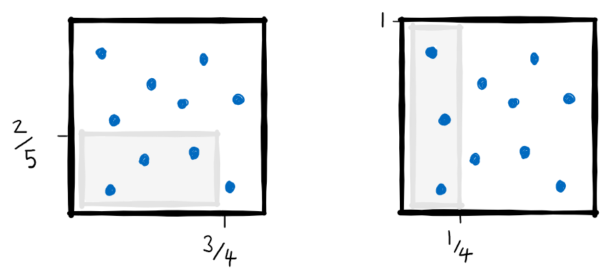
Figure 2: Star discrepancy is defined as the largest difference between the volume of a hyper-rectangle $[\bm{0},\bm{a})$ and the proportion of states $\bm{x}_{i}$ (blue dots) which are contained in the hyper-rectangle, the so-called local discrepancy at $\bm{a}\in[0,1]^{d}$. In the left hand panel, the proportion of states in the shaded hyper-rectangle is exactly equal to the volume of the hyper-rectangle, while this is not the case in the right hand panel.

Remark 1.

In dimension $d=1$ is is clear that a regular grid $\bm{x}_{1}=0$, $\bm{x}_{2}=1/(n-1)$, $\dots$, $\bm{x}_{n}=1$ minimises $D_{n}^{*}(\bm{x}_{1},\dots,\bm{x}_{n})$. In this univariate setting, you may recognise that the star discrepancy from the Kolmogorov–Smirnov uniformity test.

Remark 2.

It is simplifies discussion to anchor the hyper-rectangle at $\bm{0}$, but one can also consider an alternative to star discrepancy with hyper-rectangles $[\bm{a},\bm{b})$ that are un-anchored. This alternative discrepancy takes values in $[D_{n}^{*},2^{d}D_{n}^{*}]$, so in terms of fixed $d$ asymptotics its behaviour is identical.

Remark 3.

It may surprise you how little is known about star discrepancy. In dimensions $d\leq 2$, it has been proven that there exist a constant $0<C<\infty$ such that, for any choice of $\bm{x}_{1},\dots,\bm{x}_{n}$ and $n\in\mathbb{N}$,

$$C\frac{(\log n)^{d-1}}{n}\leq D_{n}^{*}(\bm{x}_{1},\dots,\bm{x}_{n}),$$

but for dimension $d>2$ this bound is only conjectured.

Remark 4.

There are numerous algorithms which aim to generate collections of states with small star discrepancy, including the Halton sequence, the Hammersley set, Sobol sequences, and various non-independent sampling methods, which are sometimes collectively referred to as qmc methods. For some of these methods it is known that, for an appropriate constant $0<C<\infty$ and subsequence of values $n$ in $\mathbb{N}$,

$$D_{n}^{*}(\bm{x}_{1},\dots,\bm{x}_{n})\leq C\frac{(\log n)^{d}}{n},$$

meaning that the rate of convergence in $n$ is close to the conjectured optimal rate. qmc will not be discussed further, because our aim in these lectures is to deal with more general probability distributions $P$ that arise in applications of uncertainty quantification.

Remark 5.

A regular grid consisting of of $n=m^{d}$ states does not minimise star discrepancy in dimension $d>1$. Indeed, for a regular grid (i.e. a $d$ dimensional Cartesian product of regular grids over the unit interval), one can show that

$$\frac{1}{2n^{1/d}}\leq D_{n}^{*}\leq\frac{d}{2n^{1/d}}.$$

See Leobacher and Pillichshammer (2014, Remark 2.20).

At this point it should be clear that even the simplest quantisation problems can be far from trivial. The aim of the next section is to relate the slightly abstract notion of quantisation to concrete problems of numerical integration.

Chapter Notes

The presentation of star discrepancy followed Chapter 15 of Owen (2013), which is currently a freely available online textbook. The same reference provides an excellent introduction to qmc.

2 Numerical Cubature

One of the most basic operations that one could hope to perform with a probability distribution is to compute expectations of random variables; i.e. to compute integrals of the form $\int f\mathrm{d}P$, or $\int f(\bm{x})p(\bm{x})\mathrm{d}\bm{x}$ if the probability distribution $P$ admits a pdf $p(\bm{x})$. In general such integrals do not possess a closed form and numerical integration (also called cubature) will be required. Quantisation is useful for cubature, since we can replace $P$ with a discrete approximation $\sum_{i=1}^{n}w_{i}\delta(\bm{x}_{i})$ to obtain a closed form numerical approximation $\sum_{i=1}^{n}w_{i}f(\bm{x}_{i})$ to the integral. Approximations of this form are sometimes called cubature rules. In this section we will see how star discrepancy can be used to analyse the accuracy of cubature rules in the case where $P$ is a uniform distribution on $[0,1]^{d}$.

2.1 Koksma–Hlawka Inequality

Let $\bm{x}_{\mathfrak{u}}$ denote the components of a $d$-dimensional vector $\bm{x}$ that are indexed by the set $\mathfrak{u}\subseteq\{1,\dots,d\}$. The shorthand $f(\bm{x}_{\mathfrak{u}},\bm{1})$ will be used to represent $f(\bm{y})$, where the vector $\bm{y}$ is defined by $y_{i}=x_{i}$ if $i\in\mathfrak{u}$ and otherwise $y_{i}=1$. The mixed partial derivative of $f$ with respect to each of the co-ordinates in $\mathfrak{u}$ is denoted $\partial^{|\mathfrak{u}|}f/\partial\bm{x}_{\mathfrak{u}}$, again for $\mathfrak{u}\subseteq\{1,\dots,d\}$.

Definition 3 (Variation).

For $f:[0,1]^{d}\rightarrow\mathbb{R}$ with continuous mixed partial derivatives, we define the variation of $f$ to be

$$\|f\|_{1}=\sum_{\mathfrak{u}\subseteq\{1,\dots,d\}}\int_{[0,1]^{|\mathfrak{u}|}}\left|\frac{\partial^{|\mathfrak{u}|}f}{\partial\bm{x}_{\mathfrak{u}}}(\bm{x}_{\mathfrak{u}},\bm{1})\right|\mathrm{d}\bm{x},$$

where the sum runs over all $2^{d}$ subsets $\mathfrak{u}\subseteq\{1,\dots,d\}$.

The term “variation” is overloaded in the literature and we use it only informally to give a name to the norm defined in Definition 3. The concept of variation enables the accuracy of cubature rules to be analysed:

Theorem 1 (Koksma–Hlawka inequality).

Let $f:[0,1]^{d}\rightarrow\mathbb{R}$ have continuous mixed partial derivatives. Then

$$\left|\frac{1}{n}\sum_{i=1}^{n}f(\bm{x}_{i})-\int_{[0,1]^{d}}f(\bm{x})\mathrm{d}\bm{x}\right|\leq\|f\|_{1}D_{n}^{*}(\bm{x}_{1},\dots,\bm{x}_{n}).$$ (1)

Remark 6.

The term $\|f\|_{1}$ in (1) quantifies the complexity of the integrand, while the star discrepancy quantifies the suitability of the states $\{\bm{x}_{i}\}_{i=1}^{n}$. Thus the quality of the set $\{\bm{x}_{i}\}_{i=1}^{n}$ as a quantisation of $P$ controls the accuracy of the cubature rule.

Remark 7.

The $f(\bm{1})$ term from $\|f\|_{1}$ can actually be removed, since the left hand side of (1) is invariant to $f(\bm{1})$, meaning that we can apply (1) to the function $\bm{x}\mapsto f(\bm{x})-f(\bm{1})$ instead, to obtain a tighter bound. If we do that, then we obtain (up to small technicalities) the original formulation of Koksma–Hlawka.

Later we will prove Theorem 1 in full, but for now we aim to present an elementary proof of Theorem 1 in the case $d=1$. For this we need the following:

Lemma 1.

Let $f:[0,1]\rightarrow\mathbb{R}$ be continuously differentiable and let $x_{1},\dots,x_{n}\in[0,1]$. Then

$$\frac{1}{n}\sum_{i=1}^{n}f(x_{i})-\int_{0}^{1}f(x)\mathrm{d}x=-\int_{0}^{1}\Delta(x)f^{\prime}(x)\mathrm{d}x$$

where $\Delta(x)=\Delta(x;x_{1},\dots,x_{n})$ is the local discrepancy.

Proof.

Note that the regularity assumption allows us to write

$$f(x)=f(1)-\int_{x}^{1}f^{\prime}(y)\mathrm{d}y.$$ (2)

Substituting (2) into the expression for the cubature error, we obtain

$$\frac{1}{n}\sum_{i=1}^{n}f(x_{i})-\int_{0}^{1}f(x)\mathrm{d}x =\int_{0}^{1}\int_{x}^{1}f^{\prime}(y)\mathrm{d}y\mathrm{d}x-\frac{1}{n}\sum_{i=1}^{n}\int_{x_{i}}^{1}f^{\prime}(y)\mathrm{d}y$$

$$=\int_{0}^{1}\int_{0}^{y}f^{\prime}(y)\mathrm{d}x\mathrm{d}y-\int_{0}^{1}\frac{1}{n}\sum_{i=1}^{n}\mathbbm{1}_{(x_{i},1]}(y)f^{\prime}(y)\mathrm{d}y$$

$$=\int_{0}^{1}f^{\prime}(y)\underbrace{\left[y-\frac{1}{n}\sum_{i=1}^{n}\mathbbm{1}_{(x_{i},1]}(y)\right]}_{=-\Delta(y)}\mathrm{d}y$$

as required. ∎

Proof of Theorem 1 ($d=1$).

From Lemma 1 we have

$$\left|\frac{1}{n}\sum_{i=1}^{n}f(x_{i})-\int_{0}^{1}f(x)\mathrm{d}x\right|\leq\int_{0}^{1}\left|\Delta(x)f^{\prime}(x)\right|\mathrm{d}x\leq\underbrace{\sup_{x\in[0,1]}|\Delta(x)|}_{=D_{n}^{*}}\underbrace{\int_{0}^{1}\left|f^{\prime}(x)\right|\mathrm{d}x}_{=\|f\|_{1}-|f(1)|},$$

as required. ∎

Chapter Notes

See Remark 2.19 in Dick and Pillichshammer (2010) for a detailed discussion of how Theorem 1 relates to the original formulation of Koksma and Hlawka. Lemma 1 and the proof of Theorem 1 for $d=1$ can be found in Section 2.2 in Dick and Pillichshammer (2010); see also Theorem 15.1 in Owen (2013). The one-dimensional version of the Koksma–Hlawka inequality is sometimes called Koksma’s inequality or Zaremba’s identity (Dick and Pillichshammer, 2010, p18).

2.2 Cubature Error Representer

In this section and the next, we will introduce the mathematical tools that are needed to prove Theorem 1 in full. These tools will also be useful later, when we consider practical algorithms for quantisation of general probability distributions $P$. The aim is to generalise the concept of variation in Definition 3, to allow for functions $f$ of different regularity to be integrated.

The basic idea is as follows: we consider the set $\mathcal{S}(k)$ of all functions of the form $f(\bm{x})=\sum_{i=1}^{m}b_{i}k(\bm{x},\bm{y}_{i})$, where $k$ is to be specified, the $\bm{y}_{i}$ are fixed states, and $n\in\mathbb{N}$. The function $k$ determines the regularity of the elements in $\mathcal{S}(k)$; for example, if $k(\bm{x},\bm{y})=\exp(-\|\bm{x}-\bm{y}\|)$ then the elements of $\mathcal{S}(k)$ are continuous but not differentiable, while if $k(\bm{x},\bm{y})=\exp(-\|\bm{x}-\bm{y}\|^{2})$ then the elements of $\mathcal{S}(k)$ are infinitely differentiable. See Figure 3. Since we aim to perform mathematical analysis, we will want to endow the set $\mathcal{S}(k)$ with mathematical structure that we can exploit. It is clearly a vector space (over the reals) of functions when (pointwise) addition and scalar multiplication are defined. In addition to that, we will want to make use of an inner product

$$\langle f,g\rangle_{\mathcal{S}(k)}=\sum_{i=1}^{m}\sum_{j=1}^{n}b_{i}c_{j}k(\bm{y}_{i},\bm{z}_{j}),\quad f(\bm{x})=\sum_{i=1}^{m}b_{i}k(\bm{x},\bm{y}_{i}),\quad g(\bm{x})=\sum_{j=1}^{n}c_{j}k(\bm{x},\bm{z}_{j}),$$

for which we must require that $k$ is symmetric (i.e. $\langle f,g\rangle_{\mathcal{S}(k)}=\langle g,f\rangle_{\mathcal{S}(k)}$) and positive definite (i.e. $\langle f,f\rangle_{\mathcal{S}(k)}>0$ for all $f\neq 0$). This inner product is useful because it satisfies a reproducing property, meaning that

$$\langle f,k(\cdot,\bm{x})\rangle_{\mathcal{S}(k)}=f(\bm{x}),$$

and suggesting the formal manipulation

$$\frac{1}{n}\sum_{i=1}^{n}f(\bm{x}_{i})-\int_{[0,1]^{d}}f(\bm{x})\mathrm{d}\bm{x} =\frac{1}{n}\sum_{i=1}^{n}\langle f,k(\cdot,\bm{x}_{i})\rangle_{\mathcal{S}(k)}-\int_{[0,1]^{d}}\langle f,k(\cdot,\bm{y})\rangle_{\mathcal{S}(k)}\mathrm{d}\bm{y}$$

$$\stackrel{{\scriptstyle?}}{{=}}\Bigg{\langle}f,\underbrace{\frac{1}{n}\sum_{i=1}^{n}k(\cdot,\bm{x}_{i})-\int_{[0,1]^{d}}k(\cdot,\bm{y})\mathrm{d}\bm{y}}_{=e(\cdot)}\Bigg{\rangle}_{\mathcal{S}(k)},$$

where $e(\cdot)$ is referred to as the representer of the cubature error. The representer $e(\cdot)$ would completely characterise the error of the (un-weighted) cubature rule based on the states $\{\bm{x}_{i}\}_{i=1}^{n}$. For example, if $e(\bm{x})=0$ for all $\bm{x}$ then the cubature rule would be exact for all integrands $f\in\mathcal{S}(k)$.

Unfortunately the inner product space $\mathcal{S}(k)$ is not complete, in the sense that limits of functions of the form $f(\bm{x})=\sum_{i=1}^{m}b_{i}k(\bm{x},\bm{y}_{i})$ need not be elements of the set $\mathcal{S}(k)$. In particular, the integral $\int_{[0,1]^{d}}k(\cdot,\bm{y})\mathrm{d}\bm{y}$ is not an element of $\mathcal{S}(k)$, meaning that the formal manipulation above is not well-defined. For this technical reason we work with a larger set $\mathcal{H}(k)$, called the completion of $\mathcal{S}(k)$, whose definition we present next.

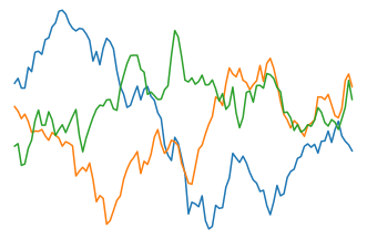
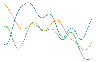
Figure 3: rkhs: The left panel represents elements from a rkhs whose kernel is non-differentiable, while the right panel corresponds to an infinitely differentiable kernel.

2.3 Reproducing Kernel Hilbert Spaces

The main mathematical tool that we will exploit is that of a reproducing kernel:

Definition 4 (Reproducing kernel Hilbert space).

Let $\mathcal{X}$ be a set and consider a symmetric and positive definite function $k:\mathcal{X}\times\mathcal{X}\rightarrow\mathbb{R}$. Then a rkhs with reproducing kernel (or simply kernel) $k$ is an inner product space $\mathcal{H}(k)$ of functions $f:\mathcal{X}\rightarrow\mathbb{R}$, such that

1. $k(\cdot,\bm{x})\in\mathcal{H}(k)$ for all $\bm{x}\in\mathcal{X}$

2. $\langle f,k(\cdot,\bm{x})\rangle_{\mathcal{H}(k)}=f(\bm{x})$ for all $\bm{x}\in\mathcal{X}$ and all $f\in\mathcal{H}(k)$.

Remark 8.

Given a symmetric positive definite function $k$, it can be shown that there exists a unique rkhs $\mathcal{H}(k)$. Conversely, each rkhs admits a unique reproducing kernel, and that kernel is symmetric and positive definite.

In general it is difficult to characterise the inner product induced by a reproducing kernel, and hence the elements of the rkhs. However, there are a number of important cases where this can be carried out:

Example 1.

The linear span of a finite collection of functions $e_{1}(\bm{x}),\dots,e_{p}(\bm{x})$ can be endowed with the structure of an rkhs with reproducing kernel $k(\bm{x},\bm{y})=\sum_{i=1}^{p}e_{i}(\bm{x})e_{i}(\bm{y})$. The induced inner product is $\langle f,g\rangle_{\mathcal{H}(k)}=b_{1}c_{1}+\dots+b_{p}c_{p}$, where $f(\bm{x})=\sum_{i=1}^{n}b_{i}e_{i}(\bm{x})$ and $g(\bm{x})=\sum_{i=1}^{n}c_{i}e_{i}(\bm{x})$.

Example 2.

The kernel

$$k(\bm{x},\bm{y})=\prod_{i=1}^{d}\left(1+\min(1-x_{i},1-y_{i})\right),\qquad\bm{x},\bm{y}\in[0,1]^{d}$$ (3)

reproduces a Hilbert space with inner product

$$\langle f,g\rangle_{\mathcal{H}(k)}=\sum_{\mathfrak{u}\subseteq\{1,\dots,d\}}\int_{[0,1]^{s}}\frac{\partial^{|\mathfrak{u}|}f}{\partial\bm{x}_{\mathfrak{u}}}(\bm{x}_{\mathfrak{u}},\bm{1})\frac{\partial^{|\mathfrak{u}|}g}{\partial\bm{x}_{\mathfrak{u}}}(\bm{x}_{\mathfrak{u}},\bm{1})\mathrm{d}\bm{x}_{\mathfrak{u}}.$$ (4)

Standing Assumption 1.

For all reproducing kernels $k$ considered in the sequel, we assume that $(\bm{x},\bm{y})\mapsto k(\bm{x},\bm{y})$ is a continuous function.

Remark 9.

Identical manipulation to that presented in Section 2.2 shows that the (Riesz) representer of the cubature error is

$$e(\bm{x})=e(\bm{x};\bm{x}_{1},\dots,\bm{x}_{n})=\frac{1}{n}\sum_{i=1}^{n}k(\bm{x},\bm{x}_{i})-\int_{[0,1]^{d}}k(\bm{x},\bm{y})\mathrm{d}\bm{y}.$$

Note that the integral of the kernel is well-defined from 1. The interchange of integral and inner product in Section 2.2 requires justification; this will be provided later in Lemma 2.

Armed with reproducing kernels and the cubature error representer, we can now prove Theorem 1 in full. In what follows we let $\bm{x}_{i,j}$ denote the $j$th coordinate of the vector $\bm{x}_{i}$ and we let $\bm{x}_{i,\mathfrak{u}}$ denote the components of the vector $\bm{x}_{i}$ that are indexed by the set $\mathfrak{u}\subseteq\{1,\dots,d\}$.

Proof of Theorem 1.

Consider the kernel $k$ in (3);

$$k(\bm{x},\bm{y})=\prod_{i=1}^{d}\left(1+\min(1-x_{i},1-y_{i})\right)$$

and compute the cubature error representer

$$e(\bm{x}) =\frac{1}{n}\sum_{i=1}^{n}k(\bm{x},\bm{x}_{i})-\int_{[0,1]^{d}}k(\bm{x},\bm{y})\mathrm{d}\bm{y}$$

$$=\frac{1}{n}\sum_{i=1}^{n}\prod_{j=1}^{d}\left(1+\min(1-x_{i},1-\bm{x}_{i,j})\right)-\prod_{i=1}^{d}\frac{3-x_{i}^{2}}{2}.$$

Then, for $\mathfrak{u}\subseteq\{1,\dots,d\}$ and $(\bm{x}_{\mathfrak{u}},\bm{1})\notin\{\bm{x}_{1},\dots,\bm{x}_{n}\}$,

$$\frac{\partial^{|\mathfrak{u}|}e}{\partial\bm{x}_{\mathfrak{u}}}(\bm{x}_{\mathfrak{u}},\bm{1}) =(-1)^{|\mathfrak{u}|}\underbrace{\left(\frac{1}{n}\sum_{i=1}^{n}\mathbbm{1}_{[\bm{0}_{\mathfrak{u}},\bm{x}_{\mathfrak{u}})}(\bm{x}_{i,\mathfrak{u}})-\prod_{i\in\mathfrak{u}}x_{i}\right)}_{=\Delta(\bm{x}_{\mathfrak{u}},\bm{1})}.$$ (5)

The assumed regularity of $f$ ensures that $f\in\mathcal{H}(k)$. Plugging (5) into (4), we obtain

$$\frac{1}{n}\sum_{i=1}^{n}f(\bm{x}_{i})-\int_{[0,1]^{d}}f(\bm{x})\mathrm{d}\bm{x} =\langle f,e\rangle_{\mathcal{H}(k)}$$

$$=\sum_{\mathfrak{u}\subseteq\{1,\dots,d\}}(-1)^{|\mathfrak{u}|}\int_{[0,1]^{d}}\frac{\partial^{|\mathfrak{u}|}f}{\partial\bm{x}_{\mathfrak{u}}}(\bm{x}_{\mathfrak{u}},\bm{1})\Delta(\bm{x}_{\mathfrak{u}},\bm{1})\mathrm{d}\bm{x}_{\mathfrak{u}}.$$

Finally, taking absolute values and using the bound $|\Delta(\bm{x}_{\mathfrak{u}},\bm{1})|\leq\sup_{\bm{x}\in[0,1]^{d}}|\Delta(\bm{x})|=D_{n}^{*}$, we arrive at (1). ∎

Chapter Notes

There are several excellent introductions to the theory of reproducing kernels, including Wendland (2004); Berlinet and Thomas-Agnan (2011). The presentation of the Koksma–Hlawka inequality from a reproducing kernel perspective follows Section 2.4 in Dick and Pillichshammer (2010). A proof of the Koksma–Hlawka inequality, which does not require reproducing kernels, can be found as Theorem 5.5 in Chapter 2 of Kuipers and Niederreiter (1974). Example 2 can be found in Section 2.4 of Dick and Pillichshammer (2010).

3 Maximum Mean Discrepancy

Now we move beyond the uniform distribution $P=\mathcal{U}([0,1]^{d})$ and consider general probability distributions $P$ on general domains $\mathcal{X}$. The aim is to present a modern treatment of discrepancy and cubature error, that generalises the previous results.

Definition 5 (Kernel mean embedding).

For a kernel $k$ and a probability distribution $P$, we call $\mu_{P}=\int k(\cdot,\bm{x})\mathrm{d}P(\bm{x})$ the kernel mean embedding of $P$ in $\mathcal{H}(k)$, whenever it is well-defined (see Lemma 2).

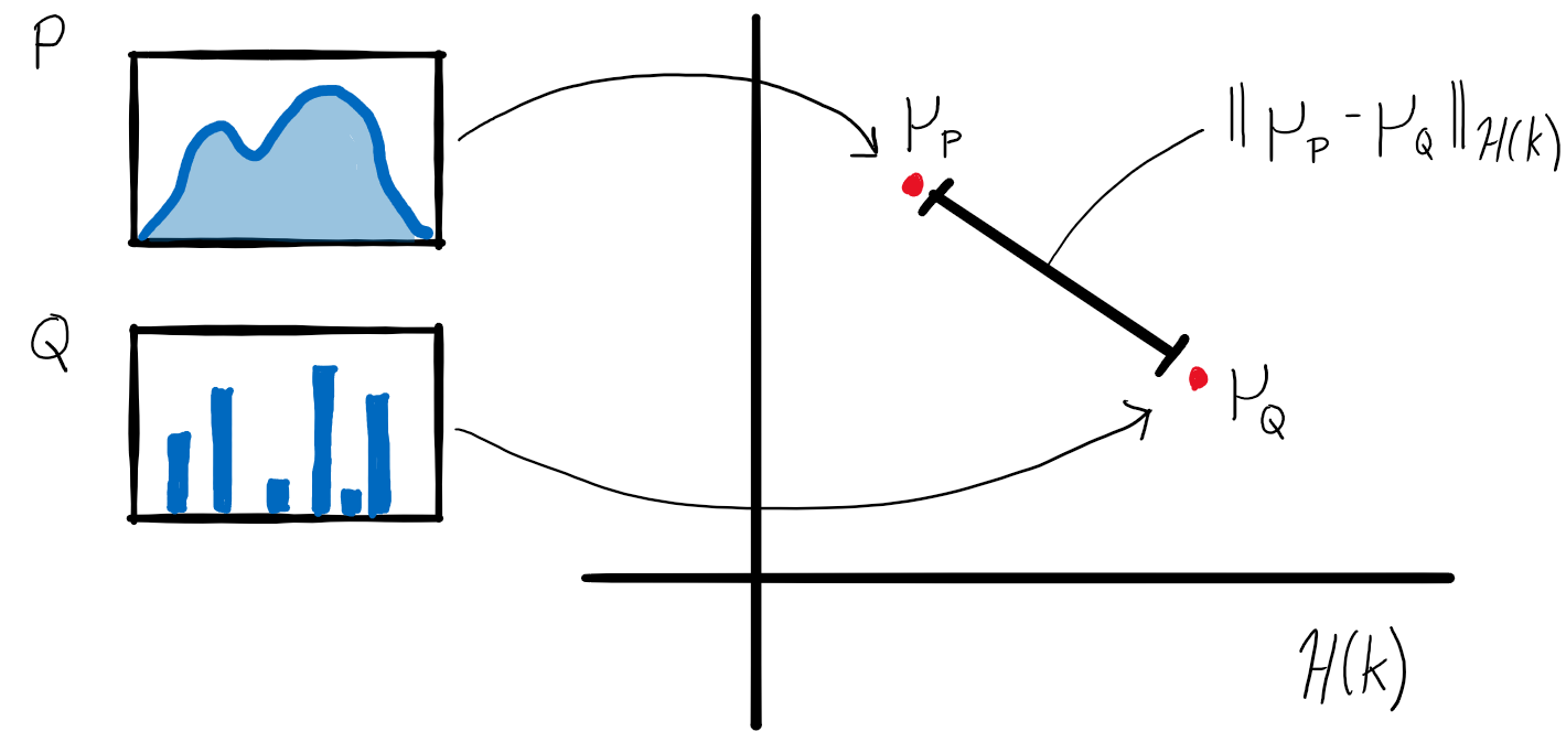
Figure 4: Kernel mean embedding: Two probability distributions $P$ and $Q$ are mapped to their respective elements $\mu_{P}$ and $\mu_{Q}$ in the rkhs $\mathcal{H}(k)$. The distance (in $\mathcal{H}(k)$) between these kernel mean embeddings $\mu_{P}$ and $\mu_{Q}$ is called the mmd between $P$ and $Q$.

Lemma 2.

If $\int\sqrt{k(\bm{x},\bm{x})}\mathrm{d}P(\bm{x})<\infty$ then $\mu_{P}(\bm{x})\in\mathcal{H}(k)$ and $\int f(\bm{x})\mathrm{d}P(\bm{x})=\langle f,\mu_{P}\rangle_{\mathcal{H}(k)}$.

Proof.

Consider the linear operator $Lf=\int f(\bm{x})\mathrm{d}P(\bm{x})$. Then

$$|Lf|=\left|\int f(\bm{x})\mathrm{d}P(\bm{x})\right| \leq\int|f(\bm{x})|\mathrm{d}P(\bm{x})$$ (6)

$$=\int|\langle f,k(\cdot,\bm{x})\rangle_{\mathcal{H}(k)}|\mathrm{d}P(\bm{x})$$ (7)

$$\leq\int\|f\|_{\mathcal{H}(k)}\|k(\cdot,\bm{x})\|_{\mathcal{H}(k)}|\mathrm{d}P(\bm{x})$$ (8)

$$=\int\sqrt{k(\bm{x},\bm{x})}\mathrm{d}P(\bm{x})\|f\|_{\mathcal{H}(k)}$$

where (6) is Jensen’s inequality, (7) is the reproducing property, and (8) is Cauchy–Schwarz. This shows that $L$ is a bounded linear operator from $\mathcal{H}(k)$ to $\mathbb{R}$. Thus, from the Riesz representation theorem, there exists $h\in\mathcal{H}(k)$ such that $Lf=\langle f,h\rangle_{\mathcal{H}(k)}$. Taking $f(\bm{x})=k(\bm{y},\bm{x})$ and using the reproducing property leads to $\int k(\bm{y},\bm{x})\mathrm{d}P(\bm{x})=Lf=\langle f,h\rangle_{\mathcal{H}(k)}=h(\bm{y})$, so that $h=\int k(\cdot,\bm{x})\mathrm{d}P(\bm{x})$, and so $\mu_{p}=h\in\mathcal{H}(k)$ with $Lf=\langle f,\mu_{P}\rangle_{\mathcal{H}(k)}$, as was claimed. ∎

Standing Assumption 2.

For all reproducing kernels $k$ and probability distributions $P$ considered in the sequel, we assume that $\int\sqrt{k(\bm{x},\bm{x})}\mathrm{d}P(\bm{x})<\infty$.

In this more general setting the Riesz representer of the cubature error is the difference $e=\mu_{Q_{n}}-\mu_{P}$ of two kernel mean embeddings, where $Q_{n}=\sum_{i=1}^{n}w_{i}\delta(\bm{x}_{i})$ is the discrete distribution on which the cubature rule is based. i.e.

$$\sum_{i=1}^{n}w_{i}f(\bm{x}_{i})-\int f\mathrm{d}P=\langle f,\mu_{Q_{n}}-\mu_{P}\rangle_{\mathcal{H}(k)},\quad\mu_{Q_{n}}=\sum_{i=1}^{n}w_{i}k(\cdot,\bm{x}_{i}),\quad\mu_{P}=\int k(\cdot,\bm{x})\mathrm{d}P(\bm{x}).$$

There are several different ways to systematically assess the performance of a cubature rule, but here we focus on a worst case assessment:

Definition 6 (Maximum mean discrepancy).

The mmd between two distributions $P$ and $Q$ is

$$D_{k}(P,Q) =\sup_{\|f\|_{\mathcal{H}(k)}\leq 1}\left|\int f\mathrm{d}P-\int f\mathrm{d}Q\right|,$$

also called the worst case cubature error in the unit ball of $\mathcal{H}(k)$.

A similar argument to Remark 9 shows that:

Lemma 3.

$D_{k}(P,Q)=\|\mu_{P}-\mu_{Q}\|_{\mathcal{H}(k)}$.

Proof.

Since $e=\mu_{P}-\mu_{Q}$ is the Riesz representer of the intergal approximation error, we may apply Cauchy–Schwarz to obtain

$$\left|\int f\mathrm{d}P-\int f\mathrm{d}Q\right|=|\langle f,e\rangle_{\mathcal{H}(k)}|\leq\|f\|_{\mathcal{H}(k)}\|e\|_{\mathcal{H}(k)},$$

which shows that

$$0\leq D_{k}(P,Q)=\sup_{\|f\|_{\mathcal{H}(k)}\leq 1}\left|\int f\mathrm{d}P-\int f\mathrm{d}Q\right|\leq\|e\|_{\mathcal{H}(k)}.$$

If $\|e\|_{\mathcal{H}(k)}=0$ then the bound is necessarily an equality. If not, consider $f=e/\|e\|_{\mathcal{H}(k)}$, which satisfies $\|f\|_{\mathcal{H}(k)}\leq 1$ and $\langle f,e\rangle_{\mathcal{H}(k)}=\|e\|_{\mathcal{H}(k)}$, showing that the bound is in fact an equality. ∎

This result is summarised visually in Figure 4.

If $D_{k}(P,Q_{n})=0$, the cubature rule based on $Q_{n}$ will be exact for all integrands $f\in\mathcal{H}(k)$. Does this mean that $Q_{n}$ and $P$ are identical?

Definition 7 (Characteristic kernel).

A kernel $k$ is said to be characteristic if $D_{k}(P,Q)=0$ implies $P=Q$.

Example 3 (Polynomial kernel is not characteristic).

From Example 1, the kernel $k(x,y)=\sum_{i=1}^{p}x^{i}y^{i}$ reproduces an rkhs whose elements are the polynomials of degree at most $p$ on the domain $\mathcal{X}=\mathbb{R}$. Thus $D_{k}(P,Q)=0$ if and only if the moments $\int x^{i}\mathrm{d}P(x)$ and $\int x^{i}\mathrm{d}Q(x)$ are identical for $i=1,\dots,p$. In particular, $k$ is not a characteristic kernel.

Example 4.

The Gaussian kernel $k(\bm{x},\bm{y})=\exp(-\|\bm{x}-\bm{y}\|^{2})$ is a characteristic kernel on $\mathcal{X}=\mathbb{R}^{d}$.

The characteristic property is desirable but, on its own, it does not provide strong justification for using $D_{k}(P,Q)$ to measure the discrepancy between $P$ and $Q$. For this reason we now introduce a stronger property, called weak convergence control. Let $Q_{n}\Rightarrow P$ denote that the sequence $(Q_{n})_{n=1}^{\infty}$ converges weakly (or in distribution) to $P$ (i.e. $\int f\mathrm{d}Q_{n}\rightarrow\int f\mathrm{d}P$ for all functions $f$ which are continuous and bounded).

Definition 8 (Weak convergence control).

A kernel $k$ is said to have weak convergence control if $D_{k}(P,Q_{n})\rightarrow 0$ implies that $Q_{n}\Rightarrow P$.

Remark 10.

Perhaps surprisingly, for a compact Hausdorff space $\mathcal{X}$, a bounded characteristic kernel $k$ is guaranteed to have weak convergence control. This equivalence no longer holds when the domain $\mathcal{X}$ is non-compact, and a bounded and characteristic kernel can fail to have weak convergence control; see Simon-Gabriel et al. (2020). Clearly a kernel that is not characteristic fails to have weak convergence control.

Convergence control justifies attempting to minimise mmd for the purposes of quantisation and more general approximation, as we will attempt in the sequel.

Example 5.

The Gaussian kernel $k(\bm{x},\bm{y})=\exp(-\|\bm{x}-\bm{y}\|^{2})$ controls weak convergence of probability distributions on $\mathcal{X}=[0,1]^{d}$. It can also be shown that the Gaussian kernel controls weak convergence on $\mathcal{X}=\mathbb{R}^{d}$; this can be deduced from e.g. Theorem 7 of Simon-Gabriel et al. (2020) and the general results in Sriperumbudur et al. (2011).

3.1 Optimal Quantisation

The goal of quantisation is to find $Q$ of the form $Q_{n}=\frac{1}{n}\sum_{i=1}^{n}\delta(\bm{x}_{i})$ such that $Q_{n}\approx P$ in some sense, and in these lectures that sense will be MMD. To start to move toward practical algorithms, notice that Lemma 3 provides a means to compute mmd:

$$D_{k}(P,Q)^{2} =\|\mu_{P}-\mu_{Q}\|_{\mathcal{H}(k)}^{2}$$

$$=\langle\mu_{P}-\mu_{Q},\mu_{P}-\mu_{Q}\rangle_{\mathcal{H}(k)}$$

$$=\langle\mu_{P},\mu_{P}\rangle_{\mathcal{H}(k)}-2\langle\mu_{P},\mu_{Q}\rangle_{\mathcal{H}(k)}+\langle\mu_{Q},\mu_{Q}\rangle_{\mathcal{H}(k)}$$

Now, considering for example the term $\langle\mu_{P},\mu_{Q}\rangle_{\mathcal{H}(k)}$, we have

$$\langle\mu_{P},\mu_{Q}\rangle_{\mathcal{H}(k)} =\left\langle\int k(\cdot,\bm{x})\mathrm{d}P(\bm{x}),\int k(\cdot,\bm{y})\mathrm{d}Q(\bm{y})\right\rangle_{\mathcal{H}(k)}$$

$$=\iint\langle k(\cdot,\bm{x}),k(\cdot,\bm{y})\rangle_{\mathcal{H}(k)}\mathrm{d}P(\bm{x})\mathrm{d}Q(\bm{y})$$

$$=\iint k(\bm{x},\bm{y})\mathrm{d}P(\bm{x})\mathrm{d}Q(\bm{y}).$$

Here we have used the reproducing property, as well as using Lemma 2 to justify the exchanges of integral and inner product. Proceeding similarly with all three terms results in the expression

$$D_{k}(P,Q)^{2} =\iint k(\bm{x},\bm{y})\mathrm{d}P(\bm{x})\mathrm{d}P(\bm{y})-2\iint k(\bm{x},\bm{y})\mathrm{d}P(\bm{x})\mathrm{d}Q(\bm{y})+\iint k(\bm{x},\bm{y})\mathrm{d}Q(\bm{x})\mathrm{d}Q(\bm{y}).$$

As a simple baseline method for quantisation we consider Monte Carlo (Figure 5):

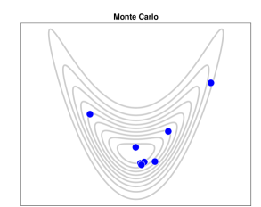
Figure 5: Monte Carlo: Independent samples (blue circles) from a “horseshoe” distribution $P$ (grey contours).

Proposition 1 (MMD of Monte Carlo).

Let $\bm{x}_{1},\dots,\bm{x}_{n}\sim P$ be independent. Assume that $C:=\int k(\bm{x},\bm{x})\mathrm{d}P(\bm{x})<\infty$. Then

$$\mathbb{E}\left[D_{k}(P,Q_{n})^{2}\right]\leq\frac{C}{n}.$$

Proof.

From the above discussion, with $Q=Q_{n}=\frac{1}{n}\sum_{i=1}^{n}\delta(\bm{x}_{i})$ we obtain that

$$D_{k}(P,Q_{n})^{2}=\iint k(\bm{x},\bm{y})\mathrm{d}P(\bm{x})\mathrm{d}P(\bm{y})-\frac{2}{n}\sum_{i=1}^{n}\int k(\bm{x},\bm{x}_{i})\mathrm{d}P(\bm{x})+\frac{1}{n^{2}}\sum_{i=1}^{n}\sum_{j=1}^{n}k(\bm{x}_{i},\bm{x}_{j})$$

Taking expectations of both sides gives

$$\mathbb{E}\left[D_{k}(P,Q_{n})^{2}\right] =\mathbb{E}\left[\frac{1}{n^{2}}\sum_{i=1}^{n}\sum_{j=1}^{n}k(\bm{x}_{i},\bm{x}_{j})\right]-\iint k(\bm{x},\bm{y})\mathrm{d}P(\bm{x})\mathrm{d}P(\bm{y})$$

$$=\mathbb{E}\left[\frac{1}{n^{2}}\sum_{i=1}^{n}k(\bm{x}_{i},\bm{x}_{i})+\frac{1}{n^{2}}\sum_{i=1}^{n}\sum_{j\neq i}k(\bm{x}_{i},\bm{x}_{j})\right]-\iint k(\bm{x},\bm{y})\mathrm{d}P(\bm{x})\mathrm{d}P(\bm{y})$$

$$=\mathbb{E}\left[\frac{1}{n^{2}}\sum_{i=1}^{n}k(\bm{x}_{i},\bm{x}_{i})\right]-\underbrace{\frac{1}{n}\iint k(\bm{x},\bm{y})\mathrm{d}P(\bm{x})\mathrm{d}P(\bm{y})}_{\geq 0}$$

$$\leq\frac{1}{n}\int k(\bm{x},\bm{x})\mathrm{d}P(\bm{x})$$

since $\bm{x}_{i}\sim P$ are independent. ∎

Thus Monte Carlo sampling provides a consistent but potentially far from optimal quantisation of $P$. Note that the convergence rate in Proposition 1 does not depend on the kernel $k$, which highlights the inefficiency of the Monte Carlo method in this context (e.g. compare against the later Theorem 2). The goal of optimal quantisation is to quantise $P$ using as few states $\bm{x}_{i}$ as possible (for a given approximation quality). A conceptually simple approach to optimal quantisation is illustrated in Figure 6, and you are encouraged to try this out:

Exercise 1 (Optimal quantisation with MMD).

Consider $P=\mathcal{N}(\bm{0},\bm{I})$ and $k(\bm{x},\bm{y})=\exp(-\|\bm{x}-\bm{y}\|^{2}/\sigma^{2})$ on $\mathcal{X}=\mathbb{R}^{d}$. (You may wish to focus on $d=1$ or $d=2$.)

1. Calculate (analytically) the kernel mean embedding $\mu_{P}(\bm{x})=\int k(\bm{x},\bm{y})\mathrm{d}P(\bm{y})$.

2. For a fixed value of $n$ (e.g. $n=10$) and a fixed value of $\sigma$ (e.g. $\sigma=1$), try to numerically optimise the locations of the states $\bm{x}_{1},\dots,\bm{x}_{n}$ in order to minimise $D_{k}(P,\frac{1}{n}\sum_{i=1}^{n}\delta(\bm{x}_{i}))$.

3. What effect does varying the bandwidth parameter $\sigma$ have on the approximations that are produced?

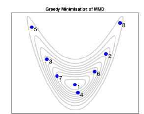
Figure 6: Optimal (un-weighted) quantisation: Sequential (greedy) minimisation of mmd to select $n=8$ states $\{\bm{x}_{i}\}_{i=1}^{n}$ in an approximation $Q_{n}$ to $P$. The numbers indicate the order in which the states $\bm{x}_{i}$ were selected.

After performing 1, it should be clear that (1) mmd provides a coherent framework for optimal quantisation, but (2) direct/naive numerical optimisation of mmd may be impractical, or at least not straight forward. A neat solution is proposed next.

3.2 Optimal Approximation

Motivated by the difficulty of multivariate optimisation in $\mathcal{X}\times\dots\times\mathcal{X}$ in 1, in this section we return to the case of independently sampled $\bm{x}_{i}\sim P$ but now we allow for weighted point sets; i.e. approximations of the form $Q_{n}=\sum_{i=1}^{n}w_{i}\delta(\bm{x}_{i})$ for some weights $w_{1},\dots,w_{n}\in\mathbb{R}$.

Lemma 4.

Let $\bm{x}_{1},\dots,\bm{x}_{n}\in\mathcal{X}$ be distinct. The optimal weights

$$\operatorname*{arg\,min}_{\bm{w}\in\mathbb{R}^{n}}D_{k}\left(P,\sum_{i=1}^{n}w_{i}\delta(\bm{x}_{i})\right)$$

are the solution of the linear system

$$\bm{K}\bm{w} =\bm{z}$$ (9)

where $K_{ij}=k(\bm{x}_{i},\bm{x}_{j})$ and $z_{i}=\mu_{P}(\bm{x}_{i})$.

Proof.

The mmd between $P$ and $Q_{n}=\sum_{i=1}^{n}w_{i}\delta(\bm{x}_{i})$ can be expressed as

$$D_{k}(P,Q_{n})^{2} =\iint k(\bm{x},\bm{y})\mathrm{d}P(\bm{x})\mathrm{d}P(\bm{y})-2\iint k(\bm{x},\bm{y})\mathrm{d}P(\bm{x})\mathrm{d}Q(\bm{y})+\iint k(\bm{x},\bm{y})\mathrm{d}Q(\bm{x})\mathrm{d}Q(\bm{y})$$

$$=C-2\bm{z}^{\top}\bm{w}+\bm{w}^{\top}\bm{K}\bm{w}$$

where $C=\iint k(\bm{x},\bm{y})\mathrm{d}P(\bm{x})\mathrm{d}P(\bm{y})$ is independent of $\bm{w}$. This is a non-degenerate quadratic form in $\bm{w}$ (since $\bm{K}$ is a positive definite matrix), from which the result is easily verified (e.g. differentiate w.r.t. $\bm{w}$ and solve for the unique critical point). ∎

See the illustration in Figure 7.

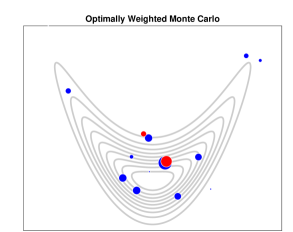
Figure 7: Optimally weighted Monte Carlo samples: The weights $w_{1},\dots,w_{n}$ are obtained by minimising mmd in the manner of Lemma 4. Blue indicates states $\bm{x}_{i}$ with positive weights $w_{i}>0$, while red indicates negative weights $w_{i}<0$. The size of the circles is proportional to $|w_{i}|$.

Remark 11.

The linear system in (9), defining the optimal weights, can be numerically ill-conditioned (i.e. close to singular) when $n$ is large or when two of the $\bm{x}_{i}$ are close together (where the terms “large” and “close” depend on the specific kernel $k$ that is used). (Of course, if $\bm{x}_{i}$ and $\bm{x}_{j}$ are identical we may assign $w_{i}=0$ without loss of generality.) Although we will not discuss this point further, there are several techniques for numerical regularisation could be used.

Remark 12.

In general the optimal weights can be negative and will not sum to $1$. Both constraints can be enforced if required and, essentially, the results that we discuss continue to hold. See e.g. Section 2.3 of Karvonen et al. (2018).

Our aim in the remainder of this section is to show that the optimal weights in Lemma 4 enable faster rates of convergence than the Monte Carlo rate in Proposition 1. To make this concrete we consider a particularly natural class of rkhs, introduced next. The multi-index notation

$$\partial^{\bm{\alpha}}f:\bm{x}\mapsto\frac{\partial^{\bm{\alpha}}f(\bm{x})}{\partial\bm{x}^{\bm{\alpha}}}=\frac{\partial^{\|\bm{\alpha}\|_{1}}}{\partial x_{1}^{\alpha_{1}}\dots\partial x_{d}^{\alpha_{d}}}f(\bm{x}),\qquad\bm{\alpha}\in\mathbb{N}_{0}^{d}$$

will be used, and we let $|\bm{\alpha}|=\alpha_{1}+\dots+\alpha_{d}$.

Definition 9.

For $s>d/2$ and (sufficiently regular) $\mathcal{X}\subset\mathbb{R}^{d}$, the (order $s$) Sobolev space $H^{s}(\mathcal{X})$ is defined to be the set of functions $f:\mathcal{X}\rightarrow\mathbb{R}$ whose mixed partial derivatives $\partial^{\bm{\alpha}}f$, $|\bm{\alpha}|\leq s$, exist in $L^{2}(\mathcal{X})$. This becomes a Hilbert space with inner product

$$\langle f,g\rangle_{H^{s}(\mathcal{X})}=\sum_{|\bm{\alpha}|\leq s}\int\frac{\partial^{\bm{\alpha}}f(\bm{x})}{\partial\bm{x}^{\bm{\alpha}}}\frac{\partial^{\bm{\alpha}}g(\bm{x})}{\partial\bm{x}^{\bm{\alpha}}}\mathrm{d}\bm{x}.$$

A kernel $k:\mathcal{X}\times\mathcal{X}\rightarrow\mathbb{R}$ is called a Sobolev kernel if there exists $0<c_{1}<c_{2}<\infty$ such that, for all $f\in\mathcal{H}(k)$, we have $c_{1}\|f\|_{H^{s}(\mathcal{X})}\leq\|f\|_{\mathcal{H}(k)}\leq c_{2}\|f\|_{H^{s}(\mathcal{X})}$.

Example 6.

Let $z_{+}^{m}$ denote $\max(0,z)^{m}$ in shorthand. Then examples of Sobolev kernels on (sufficiently regular) $\mathcal{X}\subseteq\mathbb{R}$ include the following, due to Wendland (1998):

$k(x,y)$     ($r=|x-y|$, $x,y\in\mathbb{R}$)	order
$(1-r)_{+}$	$s=1$
$(1-r)_{+}^{3}(3r+1)$	$s=2$
$(1-r)_{+}^{5}(8r^{2}+5r+1)$	$s=3$

These kernels are convenient for numerical reasons, due to their compact support, which renders $\bm{K}$ a sparse matrix.

The above inner product should be contrasted with that in Example 2. Here we are considering mixed partial derivatives of order at most $s$, where each coordinate can in principle be differentiated more than once, whereas in Example 2 we consider mixed partial derivatives of up to order $d$, provided that each coordinate of $\bm{x}$ is differentiated at most once.

Given the slow convergence of mmd with uniformly-weighted random samples in Proposition 1, the following is possibly very surprising:

Theorem 2.

Let $\bm{x}_{1},\dots,\bm{x}_{n}\sim P$ be independent and let $\bm{w}=\bm{w}(\bm{x}_{1},\dots,\bm{x}_{n})$ denote optimal weights in the sense of Lemma 4. Let $k(\bm{x},\bm{y})$ be an (order $s$) Sobolev kernel. Then, under regularity conditions on the domain $\mathcal{X}$, which is of dimension $d$, and the distribution $P$, there exists a constant $0<C<\infty$ such that

$$\mathbb{E}\left[D_{k}\left(P,\sum_{i=1}^{n}w_{i}\delta(\bm{x}_{i})\right)\right]\leq\left(\frac{C\log(n)}{n}\right)^{s/d}.$$

Proof.

The following is a sketch: For simplicity assume that $\mathcal{H}(k)$ and $H^{s}(\mathcal{X})$ have an identical inner product. Under regularity conditions on the domain $\mathcal{X}$, which amounts to $\mathcal{X}$ being bounded and satisfying an interior cone condition, one can obtain a sampling inequality of the form

$$\|f-f_{n}\|_{\infty}\leq Ch_{n}^{s/d}\|f\|_{H^{s}(\mathcal{X})}$$

where $f_{n}(\bm{x})=\sum_{i=1}^{n}c_{i}k(\bm{x},\bm{x}_{i})$, $\bm{c}=\bm{K}^{-1}\bm{f}$, is an interpolant of the function $f$ at the locations $\bm{x}_{1},\dots,\bm{x}_{n}$, and $h_{n}$ is the fill distance

$$h_{n}=\sup_{\bm{x}\in\mathcal{X}}\;\min_{i=1,\dots,n}\|\bm{x}-\bm{x}_{i}\|,$$

see e.g. Theorem 11.13 of Wendland (2004). Then observe that $\int f_{n}\mathrm{d}P=\sum_{i=1}^{n}c_{i}z_{i}=\bm{f}^{\top}\bm{K}^{-1}\bm{z}=\bm{f}^{\top}\bm{w}=\sum_{i=1}^{n}w_{i}f(\bm{x}_{i})$. Thus $\left|\sum_{i=1}^{n}w_{i}f(\bm{x}_{i})-\int f\mathrm{d}P\right|=\left|\int f_{n}\mathrm{d}P-\int f\mathrm{d}P\right|\leq\|f_{n}-f\|_{\infty}\leq Ch_{n}^{s/d}\|f\|_{H^{s}(\mathcal{X})}$. From the definition of mmd it follows that $D_{k}(P,\sum_{i=1}^{n}w_{i}f(\bm{x}_{i}))\leq Ch_{n}^{s/d}$. Under regularity conditions on $P$, which amounts to $P$ admitting a pdf bounded away from 0 and $\infty$ on $\mathcal{X}$, one can show that $\mathbb{E}[h_{n}^{s/d}]$ decreases at the advertised $\mathcal{O}(((\log n)/n)^{s/d})$ rate; see Reznikov and Saff (2016). ∎

Thus for $s=d/2$ we recover the same rate as Proposition 1 for un-weighted Monte Carlo (up to log factors), while for $s>d/2$ we obtain faster convergence in mmd.

Remark 13.

Stronger concentration inequalities than Theorem 2 can also be established; see e.g. Ehler et al. (2019).

So surely it is a good idea to employ optimal weights? Not necessarily - the computational cost is $\mathcal{O}(n^{3})$ in general and numerical ill-conditioning requires careful treatment. In qmc an important goal is to find a deterministic sequence of sets of (un-weighted) states whose computation is $\mathcal{O}(n)$, such that mmd is asymptotically minimised. Thus, at least for the simple forms of $P$ for which a qmc method has been discovered, the qmc approach would usually be preferred. The rkhs/mmd perspective on qmc was popularised by Hickernell (1998).

Exercise 2 (Rates of convergence and MMD).

Consider the uniform distribution $P=\mathcal{U}([0,1])$ together with the Sobolev kernels $k$ of orders $s\in\{1,2,3\}$ in Example 6.

1. Calculate the kernel mean embeddings $\mu_{P}(x)=\int_{0}^{1}k(x,y)\mathrm{d}y$.

2. Generate and store a sequence $(x_{i})_{i=1}^{100}$ of independent samples from $P$.

3. For each $n=1,\dots,100$ and each $s=1,2,3$, calculate and plot the values of

   $$D_{k}\left(P,\frac{1}{n}\sum_{i=1}^{n}\delta(x_{i})\right)\qquad\text{and}\qquad D_{k}\left(P,\sum_{i=1}^{n}w_{i}^{(n)}\delta(x_{i})\right)$$

   where $\bm{w}^{(m)}=(w_{1}^{(m)},\dots,w_{n}^{(m)})$ are the optimal weights obtained by solving the $m$-dimensional linear system in Lemma 4, based on the states $\{x_{i}\}_{i=1}^{m}$.

4. What rates of convergence would you expect to observe for these quantities as $n\rightarrow\infty$, and do your experiments agree with these rates of convergence?

Chapter Notes

The presentation of Lemma 2 follows Lemma 3.1 of Muandet et al. (2016). Lemma 2 presented an elementary argument for why kernel mean embeddings are well-defined, but a more general framework is the Bochner integral. Bochner’s criterion for integrability states that a Bochner-measurable function $F:[0,1]^{d}\rightarrow\mathcal{H}(k)$ is Bochner integrable if and only if $\int\|F(\bm{x})\|_{\mathcal{H}(k)}\mathrm{d}P(\bm{x})<\infty$. Here we take $F(\bm{x})=k(\cdot,\bm{x})$, noting that $\|k(\cdot,\bm{x})\|_{\mathcal{H}(k)}=\sqrt{k(\bm{x},\bm{x})}$, which recovers the condition in Lemma 2. There is an elegant criterion to determine when a translation-invariant kernel $k$ (i.e. $k(\bm{x},\bm{y})=\phi(\bm{x}-\bm{y})$ for some function $\phi$) is characteristic; see Section 2.1 of Muandet et al. (2016). Stronger concentration inequalities than Proposition 1 for Monte Carlo MMD have been established; see Section 3.3 of Muandet et al. (2016). The case of Theorem 2 where $\mathcal{X}$ is a smooth, connected, closed Riemannian manifold of dimension $d$ is presented in Ehler et al. (2019). (This requires some generalisation of the definition of a Sobolev kernel.) The fastest known rates for explicit constructions of weighted approximations in the case of 1 are (at the time of writing) due to Karvonen et al. (2021). Greedy optimisation can provide a practical solution to optimal quantisation problems like 1 (Pronzato and Zhigljavsky, 2020; Teymur et al., 2021), as can the sophisticated numerical methods for high-dimensional optimisation used to produce Figure 1 (Gräf et al., 2012). Several tricks are available to reduce the cost of solving the linear system in (9); see e.g. Karvonen and Särkkä (2018).

4 Stein Discrepancy

In this final section we aim to perform optimal quantisation of a distribution $P$ that admits a pdf $p(\bm{x})$ on $\bm{x}\in\mathbb{R}^{d}$, such that

$$p(\bm{x})=\frac{\tilde{p}(\bm{x})}{Z},$$

where $\tilde{p}$ can be exactly evaluated but $Z$, and hence $p(\bm{x})$, cannot easily be evaluated or even approximated. This setting is typical in applications of Bayesian inference, where we have

$$p(\bm{x})=\frac{\pi(\bm{x})\mathcal{L}(\bm{x})}{Z}$$

where $\pi(\bm{x})$ is a prior pdf, $\mathcal{L}(\bm{x})$ is a likelihood, and the implicitly defined normalisation constant $Z$ is the marginal likelihood. The integral

$$Z=\int\pi(\bm{x})\mathcal{L}(\bm{x})\mathrm{d}\bm{x}$$

is often extremely challenging to evaluate due to localised regions in which $\mathcal{L}$ takes very large values. Several methods have been developed in the statistics, applied probability, physics and machine learning literatures to approximate distributions $P$ with these characteristics, including mcmc, smc, and variational inference. These techniques do not typically attempt optimal quantisation, since even the basic quantisation task can be difficult.

The aim of this section is to discuss whether the techniques described in Section 3 can be applied in this more challenging context. The apparent difficulty is that we cannot compute integrals with respect to $P$, such as $\int k(\cdot,\bm{x})\mathrm{d}P(\bm{x})$, which are required for computation of mmd. A hint at a possible solution is provided by the following result:

Lemma 5.

Suppose $k_{P}:\mathcal{X}\times\mathcal{X}\rightarrow\mathbb{R}$ is a symmetric positive definite kernel with $\int k_{P}(\cdot,\bm{x})\mathrm{d}P=0$ for all $\bm{x}\in\mathcal{X}$. Then

$$D_{k_{P}}(Q)=D_{k_{P}}(P,Q)=\sup_{\|f\|_{\mathcal{H}(k_{P})}\leq 1}\left|\int f\mathrm{d}Q\right|.$$

Proof.

For all $f\in\mathcal{H}(k_{P})$ it holds that $\int f\mathrm{d}P=0$, whence the result. Indeed, from the reproducing property, and using Lemma 2 with 2 to interchange integral with inner product, $\int f\mathrm{d}P=\int\langle f,k(\cdot,\bm{x})\rangle_{\mathcal{H}(k_{P})}\mathrm{d}P(\bm{x})=\left\langle f,\int k(\cdot,\bm{x})\mathrm{d}P(\bm{x})\right\rangle_{\mathcal{H}(k_{P})}=\langle f,0\rangle_{\mathcal{H}(k_{P})}=0$. ∎

The important point here is that $D_{k_{P}}(Q)$ does not require integrals with respect to $P$ to be computed. A kernel $k_{P}$ with $\int k_{P}(\cdot,\bm{x})\mathrm{d}P=0$ will be called a Stein kernel (for $P$), for reasons that will become clear in the sequel. An example for how such a kernel can be constructed is as follows: Consider the bounded linear operator $(\mathcal{A}_{P}g)(\bm{x})=g(\bm{x})-\int g\mathrm{d}P$ acting on elements of an rkhs $\mathcal{H}(k)$. If we apply $\mathcal{A}_{P}$ to both arguments of the kernel $k$, we obtain a Stein kernel

$$k_{P}(\bm{x},\bm{y}) =\mathcal{A}_{P}^{\bm{y}}\mathcal{A}_{P}^{\bm{x}}k(\bm{x},\bm{y})$$

$$=k(\bm{x},\bm{y})-\int k(\bm{x},\bm{y})\mathrm{d}P(\bm{x})-\int k(\bm{x},\bm{y})\mathrm{d}P(\bm{y})+\iint k(\bm{x},\bm{y})\mathrm{d}P(\bm{x})\mathrm{d}P(\bm{y}).$$ (10)

Indeed, $\int k_{P}(\cdot,\bm{x})\mathrm{d}P(\bm{x})=\int\mathcal{A}_{P}^{\bm{y}}\mathcal{A}_{P}^{\bm{x}}k(\bm{x},\bm{y})\mathrm{d}P(\bm{x})=\mathcal{A}_{P}^{\bm{y}}\int\mathcal{A}_{P}^{\bm{x}}k(\bm{x},\bm{y})\mathrm{d}P(\bm{x})=\mathcal{A}_{P}^{\bm{y}}0=0$, where interchange of $\mathcal{A}_{P}^{\bm{y}}$ and the integral is justified by noting that $\mathcal{A}_{P}^{\bm{y}}$ is a bounded linear operator and following similar reasoning to Lemma 2. In fact, the rkhs $\mathcal{H}(k_{P})$ consists of functions of the form $\mathcal{A}_{P}g=g-\int g\mathrm{d}P$ where $g\in\mathcal{H}(k)$. Unfortunately, the Stein kernel in (10) is not useful because it still involves the problematic integral $\int k(\cdot,\bm{x})\mathrm{d}P(\bm{x})$. The next section presents a more useful construction of a Stein kernel.

4.1 Stein Operators

The aim here is to identify an alternative operator $\mathcal{A}_{P}$, which can be computed. Let $\nabla f=(\partial_{x_{1}}f,\dots,\partial_{x_{d}}f)^{\top}$ for differentiable functions $f:\mathbb{R}^{d}\rightarrow\mathbb{R}$. Our main tool is a Stein operator, and the classical example of this is as follows:

Standing Assumption 3.

The distribution $P$ admits a positive and differentiable pdf such that $\bm{x}\mapsto(\nabla\log p)(\bm{x})$ is Lipschitz.

Definition 10 (Canonical Stein operator).

For a distribution $P$ admitting a positive and differentiable density $p$ on $\mathbb{R}^{d}$, we define the canonical Stein operator

$$(\mathcal{A}_{P}g)(\bm{x})=(\nabla\cdot g)(\bm{x})+g(\bm{x})\cdot(\nabla\log p)(\bm{x})$$

acting on differentiable vector field $g:\mathbb{R}^{d}\rightarrow\mathbb{R}^{d}$, where $\bm{x}\in\mathbb{R}^{d}$.

The canonical Stein operator was introduced (for Gaussian $P$) in Stein (1972). Importantly, observe that

$$(\nabla\log p)(\bm{x})=\frac{(\nabla p)(\bm{x})}{p(\bm{x})}=\frac{\frac{1}{Z}(\nabla\tilde{p})(\bm{x})}{\frac{1}{Z}\tilde{p}(\bm{x})}=\frac{(\nabla\tilde{p})(\bm{x})}{\tilde{p}(\bm{x})}=(\nabla\log\tilde{p})(\bm{x}),$$

which can be computed without knowledge of $p$ or $Z$, provided $\tilde{p}$ and $\nabla\tilde{p}$ can be evaluated. Loosely speaking, we can apply the Stein operator $\mathcal{A}_{P}$ in Definition 10 to a standard kernel $k$ to obtain the following Stein kernel:

Lemma 6.

Suppose that $k:\mathbb{R}^{d}\times\mathbb{R}^{d}\rightarrow\mathbb{R}$ is a symmetric positive definite kernel with $(\bm{x},\bm{y})\mapsto\partial^{(\bm{\alpha},\bm{\beta})}k(\bm{x},\bm{y})$ being continuous and uniformly bounded for all $|\bm{\alpha}|,|\bm{\beta}|\leq 1$. Suppose $\int\|\nabla\log p(\bm{x})\|\mathrm{d}P(\bm{x})<\infty$ and that $\sup_{\|\bm{x}\|\geq r}r^{d-1}p(\bm{x})\rightarrow 0$ as $r\rightarrow\infty$. Then

$$k_{P}(\bm{x},\bm{y}) =\nabla_{\bm{x}}\cdot\nabla_{\bm{y}}k(\bm{x},\bm{y})+\nabla_{\bm{x}}\log p(\bm{x})\cdot\nabla_{\bm{y}}k(\bm{x},\bm{y})+\nabla_{\bm{y}}\log p(\bm{y})\cdot\nabla_{\bm{x}}k(\bm{x},\bm{y})$$

$$\qquad+(\nabla_{\bm{x}}\log p(\bm{x}))\cdot(\nabla_{\bm{y}}\log p(\bm{y}))k(\bm{x},\bm{y})$$

is a symmetric positive definite kernel with $\int k_{P}(\bm{x},\bm{y})\mathrm{d}P(\bm{y})=0$ for all $\bm{x}\in\mathbb{R}^{d}$.

Proof.

First notice that

$$k_{P}(\bm{x},\bm{y})=\mathcal{A}_{P}^{\bm{y}}\left[\begin{array}[]{c}\vdots\\ \nabla_{x_{i}}k(\bm{x},\bm{y})+k(\bm{x},\bm{y})\nabla_{x_{i}}\log p(\bm{x})\\ \vdots\end{array}\right]=\mathcal{A}_{P}^{\bm{y}}g(\bm{y})$$

where, under our assumptions, (a) $\bm{y}\mapsto g(\bm{y})$ is bounded, and (b) $\bm{y}\mapsto\nabla_{\bm{y}}\cdot g(\bm{y})$ is integrable with respect to $P$. Thus it suffices to show that $\int\mathcal{A}_{P}g\mathrm{d}P=0$ for all vector fields $g$ for which (a) and (b) hold.

Let $g$ be such a vector field, and let $B_{r}=\{\bm{x}\in\mathbb{R}^{d}:\|\bm{x}\|\leq r\}$ and $S_{r}=\{\bm{x}\in\mathbb{R}^{d}:\|\bm{x}\|=r\}$. The main idea is to apply the divergence theorem (i.e. integrate by parts):

$$\int\mathcal{A}_{P}g\mathrm{d}P =\int(\nabla\cdot g)+g\cdot(\nabla\log p)\mathrm{d}P$$

$$=\int(\nabla\cdot(pg))(\bm{x})\mathrm{d}\bm{x}$$

$$=\lim_{r\rightarrow\infty}\int_{B_{r}}(\nabla\cdot(pg))(\bm{x})\mathrm{d}\bm{x}$$

$$=\lim_{r\rightarrow\infty}\oint_{S_{r}}p(\bm{x})(g(\bm{x})\cdot n(\bm{x}))\mathrm{d}\bm{x}$$

where $n(\bm{x})$ is the outward unit normal to $S_{r}$ at $\bm{x}$. (The regularity assumptions ensure that the integrals $\int(\nabla\cdot g)\mathrm{d}P$ and $\int g\cdot(\nabla\log p)\mathrm{d}P$ exist.) Now

$$\oint_{S_{r}}p(\bm{x})(g(\bm{x})\cdot n(\bm{x}))\mathrm{d}\bm{x} \leq\|g\|_{\infty}\sup_{\|\bm{x}\|\geq r}p(\bm{x})\oint_{S_{r}}\mathrm{d}\bm{x}$$

$$=\|g\|_{\infty}\sup_{\|\bm{x}\|\geq r}p(\bm{x})\frac{2\pi^{d/2}}{\Gamma(d/2)}r^{d-1}$$

$$\rightarrow 0\text{ as }r\rightarrow\infty,$$

where we have used the formula for the surface area of the radius $r$ sphere in $\mathbb{R}^{d}$. ∎

Definition 11 (Kernel Stein discrepancy).

With $k_{P}$ defined in Lemma 6, we call $D_{k_{P}}$ in Lemma 5 a ksd.

Lemma 7.

For $Q_{n}=\sum_{i=1}^{n}w_{i}\delta(\bm{x}_{i})$, we have the explicit form of ksd:

$$D_{k_{P}}(Q_{n})=\sqrt{\sum_{i=1}^{n}\sum_{j=1}^{n}w_{i}w_{j}k_{P}(\bm{x}_{i},\bm{x}_{j})}$$

Proof.

Immediate from the closed form expression for mmd in Section 3.1, with $k_{P}$ in place of $k$ and using the fact that $\int k_{P}(\bm{x},\bm{y})\mathrm{d}P(\bm{y})=0$ for all $\bm{x}\in\mathbb{R}^{d}$ from Lemma 6. ∎

As with mmd, we can establish properties analogous to characteristicness and convergence control for ksd. Here we focus on the stronger property of convergence control:

Theorem 3.

Let $P$ be distantly dissipative, meaning that $\lim\inf_{r\rightarrow\infty}\kappa(r)>0$ where

$$\kappa(r)=\inf\left\{-2\frac{(\langle\nabla\log p)(\bm{x})-(\nabla\log p)(\bm{y}),\bm{x}-\bm{y}\rangle}{\|\bm{x}-\bm{y}\|^{2}}:\|\bm{x}-\bm{y}\|=r\right\}.$$

Consider the kernel $k(\bm{x},\bm{y})=(\sigma^{2}+\|\bm{x}-\bm{y}\|^{2})^{-\beta}$ for some fixed $\sigma>0$ and a fixed exponent $\beta\in(0,1)$. Then $D_{k_{P}}(Q_{n})\rightarrow 0$ implies $Q_{n}\Rightarrow P$.

Proof.

Theorem 8 in Gorham and Mackey (2017). ∎

Theorem 3 justifies attempting to minimise ksd from the point of view of quantisation, which we will discuss next.

4.2 Optimal Quantisation

The simplest use of ksd for quantisation is as follows:

Exercise 3 (Optimal quantisation with KSD).

Consider $P=\mathcal{N}(\bm{0},\bm{I})$ and $k(\bm{x},\bm{y})=(\sigma^{2}+\|\bm{x}-\bm{y}\|^{2})^{-1/2}$ on $\mathcal{X}=\mathbb{R}^{d}$. (You may wish to focus on $d=1$ or $d=2$.)

1. Verify that $P$ and $k$ satisfy the conditions of Theorem 3.

2. Calculate (analytically) the Stein kernel $k_{P}(\bm{x},\bm{y})$.

3. For a fixed value of $n$ (e.g. $n=10$) and a fixed value of $\sigma$ (e.g. $\sigma=1$), try to numerically optimise the locations of the states $\bm{x}_{1},\dots,\bm{x}_{n}$ in order to minimise $D_{k}(P,\frac{1}{n}\sum_{i=1}^{n}\delta(\bm{x}_{i}))$.

4. What effect does varying the bandwidth parameter $\sigma$ have on the approximations that are produced?

5. What happens if instead the Gaussian kernel $k(\bm{x},\bm{y})=\exp(-\|\bm{x}-\bm{y}\|^{2}/\sigma^{2})$ is used?

This provides an optimisation-based alternative to popular sampling-based algorithms, such as mcmc and smc. See Figure 8.

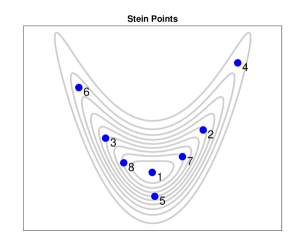
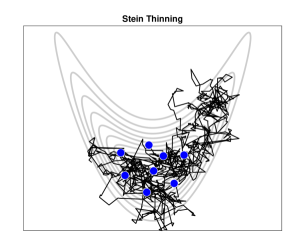
Figure 8: Stein points (left) and Stein thinning (right): Stein points are generated by sequential (greedy) minimisation of ksd to select $n=8$ states $\{\bm{x}_{i}\}_{i=1}^{n}$ in an approximation $Q_{n}$ to $P$. The numbers indicate the order in which the states $\bm{x}_{i}$ were selected. Stein thinning restricts the continuous inner-loop optimisation problem in Stein points to a discrete search over a mcmc sample path (black).

Remark 14.

The Gaussian distribution $P$ in 3 is analytically tractable, so ksd is not actually needed and mmd can be used. You are encouraged to extend 3 by replacing $P$ with an intractable posterior distribution arising in an application of Bayesian statistics.

Remark 15.

Sequential greedy optimisation provides one practical solution to part (c) of 3, and was studied in detail in Chen et al. (2018, 2019). States $\{\bm{x}_{i}\}_{i=1}^{n}$ constructed in this way were called Stein points.

4.3 Optimal Approximation

In challenging applications of Bayesian statistics, the optimisation over $\mathcal{X}$ that was required to perform 3 will be difficult. Nevertheless, approximate sampling from $P$ may still be possible using mcmc or smc. Through the optimisation of weights, Stein discrepancy provides an means to improve the approximations produced by mcmc or smc, in a similar spirit to how importance sampling is sometimes used.

However, if we were to apply Lemma 4 with the kernel $k_{P}$ in place of $k$ we would obtain a degenerate solution, since $z_{i}=\int k_{P}(\cdot,\bm{x}_{i})\mathrm{d}P=0$ and optimal weights are $\bm{w}=\bm{0}$. This makes sense, since we know that all $f\in\mathcal{H}(k_{P})$ integrate to 0. In order to make progress we need an additional constraint on the weights, and for this purpose it is natural to impose that $w_{1}+\dots+w_{n}=1$. This leads to the following extension of Lemma 4, which we present for a Stein kernel:

Lemma 8.

Let $\bm{x}_{1},\dots,\bm{x}_{n}\in\mathcal{X}$ be distinct. The optimal weights

$$\operatorname*{arg\,min}_{\begin{subarray}{c}\bm{w}\in\mathbb{R}^{n}\\ \bm{1}^{\top}\bm{w}=1\end{subarray}}D_{k_{P}}\left(\sum_{i=1}^{n}w_{i}\delta(\bm{x}_{i})\right)$$

are

$$\bm{w} =\frac{\bm{K}_{P}^{-1}\bm{1}}{\bm{1}^{\top}\bm{K}_{P}^{-1}\bm{1}}$$

where $[K_{P}]_{ij}=k_{P}(\bm{x}_{i},\bm{x}_{j})$.

Proof.

From Lemma 7 we have

$$D_{k_{P}}\left(\sum_{i=1}^{n}w_{i}\delta(\bm{x}_{i})\right)^{2}=\bm{w}^{\top}\bm{K}_{P}\bm{w},$$

so the optimisation problem is

$$\operatorname*{arg\,min}\bm{w}^{\top}\bm{K}_{P}\bm{w}\qquad\text{s.t.}\qquad\bm{1}^{\top}\bm{w}=1.$$

This can be solved using the method of Lagrange multipliers to obtain the stated result. ∎

See the left panel of Figure 9. As with optimal weights for mmd, the linear system which must be solved can be numerically ill-conditioned when $n$ is large, or when two of the $\bm{x}_{i}$ are very close or identical. Techniques for numerical regularisation could be used.

Exercise 4 (Bias correction with KSD).

Consider again the distribution $P$ and kernel $k$ from 3.

1. Generate and store a sequence $(\bm{x}_{i})_{i=1}^{100}$ of independent samples from $P$.

2. For each $n=1,\dots,100$, calculate and plot the values of

   $$D_{k}\left(P,\frac{1}{n}\sum_{i=1}^{n}\delta(\bm{x}_{i})\right)\qquad\text{and}\qquad D_{k}\left(P,\sum_{i=1}^{n}w_{i}^{(n)}\delta(\bm{x}_{i})\right)$$

   where $\bm{w}^{(m)}=(w_{1}^{(m)},\dots,w_{n}^{(m)})$ are the optimal weights from Lemma 8, based on the states $\{\bm{x}_{i}\}_{i=1}^{m}$. What do you observe?

3. What happens if, instead, we consider $n=1,\dots,1000$?

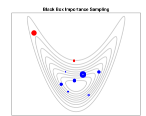
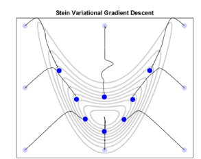
Figure 9: Black box importance sampling (left) and Stein variational gradient descent (right): In black box importance sampling the weights $w_{1},\dots,w_{n}$ are obtained by minimising ksd in the manner of Lemma 8. Blue indicates states $\bm{x}_{i}$ with positive weights $w_{i}>0$, while red indicates negative weights $w_{i}<0$. The size of the circles is proportional to $|w_{i}|$. Stein variational gradient descent (Liu and Wang, 2016) is one of a number of recently developed algorithms based on ksd; here an initial discrete distribution (light blue circles) are evolved in time (black lines) toward an optimal quantisation (dark blue circles) of $P$.

Remarkably, the use of Stein discrepancy in 4 can provide consistent approximations of $P$ even if the states $\bm{x}_{i}$, generated in step (a), are not sampled from $P$ (provided, at least, that they are sampled from a distribution that is not too different from $P$). See Liu and Lee (2017); Hodgkinson et al. (2020) and Theorem 3 of Riabiz et al. (2021). This is reminiscent of importance sampling, and Liu and Lee (2017) termed it black-box importance sampling.

Exercise 5 (Pathologies of KSD).

The purpose of this final exercise is to illustrate one of the main weaknesses of ksd; insensitivity to distant high probability regions. Consider the Gaussian mixture model

$$p(x)\propto\exp(-x^{2})+\exp(-(x-c)^{2})$$

for $c\geq 0$.

1. Calculate (analytically) the gradient $(\nabla\log p)(x)$.

2. Derive the kernel $k_{P}(x,y)$, using $k(x,y)=(1+(x-y)^{2})^{-1/2}$ (to ensure convergence control; c.f. Theorem 3).

3. Generate and store an independent sample $(x_{i})_{i=1}^{n}$ from $\mathcal{N}(0,1)$, with $n=100$.

4. Plot $D_{k_{P}}(\frac{1}{n}\sum_{i=1}^{n}\delta(x_{i}))$ as a function of $c\in(0,10)$.

5. What do you conclude about the sensitivity of ksd to distant high probability regions?

Chapter Notes

The canonical Stein operator is sometimes called the Langevin–Stein operator due to its close connection with the generator of a Langevin diffusion process (Barbour, 1988, 1990; Gorham and Mackey, 2015). The general concept of a Stein discrepancy, in Lemma 5, was introduced in Gorham and Mackey (2015). The Stein kernel was introduced in Oates et al. (2017) and ksd was later introduced simultaneously in Chwialkowski et al. (2016); Liu et al. (2016). Lemma 6 can be found in South et al. (2021). Theorem 3 was slightly generalised to allow for invertible linear transformations of $\bm{x}$ in the kernel $k$ in Theorem 4 of Chen et al. (2019). The optimal weights in Lemma 8 are numerically ill-conditioned when $n$ is large; to address this, Riabiz et al. (2021) showed that greedy subset selection can be almost as accurate, but with lower computational complexity. Stein discrepancy is an active research topic at the moment, with many extensions attracting attention, such as to non-Euclidean domains (Barp et al., 2021), to other function classes besides kernels (Si et al., 2020; Grathwohl et al., 2020), and inspiring new algorithms such as Stein variational gradient descent (Liu and Wang, 2016) (see the right panel of Figure 9). For a recent literature review, see Anastasiou et al. (2021).

5 Partial Solutions to Exercises

This section contains solutions to analytic parts of the exercises in the main text. For the numerical part of the exercises, Matlab solutions are provided.

5.1 1

(a)

In dimension $d$ we have the kernel mean embedding

$$\mu_{P}(\bm{x})=\left(\frac{\sigma^{2}}{2+\sigma^{2}}\right)^{d/2}\exp\left\{-\frac{1}{(2+\sigma^{2})}\|\bm{x}\|^{2}\right\}.$$

5.2 2

(a)

The maximum value operator $z\mapsto z_{+}$ that appears in the kernels of Example 6 is irrelevant when restricting to $\mathcal{X}=[0,1]$, since $1-|x-y|\geq 0$ for all $x,y\in[0,1]$. Thus we consider the following kernels on $\mathcal{X}=[0,1]$:

$k(x,y)$     ($r=|x-y|$, $x,y\in[0,1]$)	order
$(1-r)$	$s=1$
$(1-r)^{3}(3r+1)$	$s=2$
$(1-r)^{5}(8r^{2}+5r+1)$	$s=3$

Splitting $\int_{0}^{1}k(x,y)\mathrm{d}y$ into a sum of $\int_{0}^{x}k(x,y)\mathrm{d}{y}$ and $\int_{x}^{1}k(x,y)\mathrm{d}y$, the integrals become straight forward and we can evaluate them analytically:

order	$\mu_{P}(x)$	$\iint k(x,y)\mathrm{d}x\mathrm{d}y$
$s=1$	$-x^{2}+x+\frac{1}{2}$	$\frac{2}{3}$
$s=2$	$x^{4}-2x^{3}+x+\frac{2}{5}$	$\frac{3}{5}$
$s=3$	$-2x^{8}+8x^{7}-\frac{35}{3}x^{6}+7x^{5}-\frac{7}{3}x^{3}+x+\frac{1}{3}$	$\frac{19}{36}$

5.3 3

(b)

Let $u(\bm{x})=(\nabla\log p)(\bm{x})$ and consider the kernel $k(\bm{x},\bm{y})=(1+\|\bm{x}-\bm{y}\|^{2})^{-1/2}$. For the case where $P=\mathcal{N}(\bm{0},\bm{I})$ we have $u(\bm{x})=-\bm{x}$. Then we compute

$$\nabla_{\bm{x}}k(\bm{x},\bm{y}) =-\frac{1}{\left(1+\|\bm{x}-\bm{y}\|^{2}\right)^{3/2}}(\bm{x}-\bm{y})$$

$$\nabla_{\bm{y}}k(\bm{x},\bm{y}) =\frac{1}{\left(1+\|\bm{x}-\bm{y}\|^{2}\right)^{3/2}}(\bm{x}-\bm{y})$$

$$\nabla_{\bm{x}}\cdot\nabla_{\bm{y}}k(\bm{x},\bm{y}) =-\frac{3\|\bm{x}-\bm{y}\|^{2}}{\left(1+\|\bm{x}-\bm{y}\|^{2}\right)^{5/2}}+\frac{d}{\left(1+\|\bm{x}-\bm{y}\|^{2}\right)^{3/2}}$$

which leads to

$$k_{P}(\bm{x},\bm{y}) :=\nabla_{\bm{x}}\cdot\nabla_{\bm{y}}k(\bm{x},\bm{y})+[\nabla_{\bm{x}}k(\bm{x},\bm{y})]^{\top}u(\bm{y})+[\nabla_{\bm{y}}k(\bm{x},\bm{y})]^{\top}u(\bm{x})+k(\bm{x},\bm{y})[u(\bm{x})^{\top}u(\bm{y})]$$

$$=-\frac{3\|\bm{x}-\bm{y}\|^{2}}{\left(1+\|\bm{x}-\bm{y}\|^{2}\right)^{5/2}}+2\beta\left[\frac{d+[u(\bm{x})-u(\bm{y})]^{\top}(\bm{x}-\bm{y})}{\left(1+\|\bm{x}-\bm{y}\|^{2}\right)^{3/2}}\right]+\frac{u(\bm{x})^{\top}u(\bm{y})}{\left(1+\|\bm{x}-\bm{y}\|^{2}\right)^{1/2}}$$

(e)

Theorem 5 of Gorham and Mackey [2017] proves that the Stein kernel $k_{P}$ based on the Gaussian kernel $k$ provides weak convergence control when $P$ is distantly dissipative (and $\nabla\log p$ is Lipschitz, under 3). However, for $d\geq 3$, Theorem 6 of Gorham and Mackey [2017] proves that the corresponding ksd does not provide weak convergence control.

5.4 5

(a)

The required gradient is

$$(\nabla\log p)(x) =-2\left[\frac{x\exp(-x^{2})+(x-c)\exp(-(x-c)^{2})}{\exp(-x^{2})+\exp(-(x-c)^{2})}\right].$$

References

- Anastasiou et al. [2021] Andreas Anastasiou, Alessandro Barp, François-Xavier Briol, Bruno Ebner, Robert E Gaunt, Fatemeh Ghaderinezhad, Jackson Gorham, Arthur Gretton, Christophe Ley, Qiang Liu, Lester Mackey, Chris J Oates, Gesine Reinert, and Yvik Swan. Stein’s method meets statistics: A review of some recent developments. arXiv:2105.03481, 2021.
- Barbour [1988] Andrew D Barbour. Stein’s method and Poisson process convergence. Journal of Applied Probability, 25(A):175–184, 1988.
- Barbour [1990] Andrew D Barbour. Stein’s method for diffusion approximations. Probability Theory and Related Fields, 84(3):297–322, 1990.
- Barp et al. [2021] Alessandro Barp, Chris J Oates, Emilio Porcu, and Mark Girolami. A Riemann–Stein kernel method. Bernoulli, 2021. To appear.
- Berlinet and Thomas-Agnan [2011] Alain Berlinet and Christine Thomas-Agnan. Reproducing Kernel Hilbert Spaces in Probability and Statistics. Springer Science & Business Media, 2011.
- Chen et al. [2018] Wilson Ye Chen, Lester Mackey, Jackson Gorham, François-Xavier Briol, and Chris J Oates. Stein points. In International Conference on Machine Learning, pages 844–853. PMLR, 2018.
- Chen et al. [2019] Wilson Ye Chen, Alessandro Barp, François-Xavier Briol, Jackson Gorham, Mark Girolami, Lester Mackey, and Chris J Oates. Stein point Markov chain Monte Carlo. In International Conference on Machine Learning, pages 1011–1021. PMLR, 2019.
- Chwialkowski et al. [2016] Kacper Chwialkowski, Heiko Strathmann, and Arthur Gretton. A kernel test of goodness of fit. In International Conference on Machine Learning, pages 2606–2615. PMLR, 2016.
- Dick and Pillichshammer [2010] Josef Dick and Friedrich Pillichshammer. Digital nets and sequences: Discrepancy theory and quasi-Monte Carlo integration. Cambridge University Press, 2010.
- Ehler et al. [2019] Martin Ehler, Manuel Gräf, and Chris J Oates. Optimal Monte Carlo integration on closed manifolds. Statistics and Computing, 29(6):1203–1214, 2019.
- Gorham and Mackey [2015] Jackson Gorham and Lester Mackey. Measuring sample quality with Stein’s method. Advances in Neural Information Processing Systems, 28:226–234, 2015.
- Gorham and Mackey [2017] Jackson Gorham and Lester Mackey. Measuring sample quality with kernels. In International Conference on Machine Learning, pages 1292–1301. PMLR, 2017.
- Gräf et al. [2012] Manuel Gräf, Daniel Potts, and Gabriele Steidl. Quadrature errors, discrepancies, and their relations to halftoning on the torus and the sphere. SIAM Journal on Scientific Computing, 34(5):A2760–A2791, 2012.
- Grathwohl et al. [2020] Will Grathwohl, Kuan-Chieh Wang, Jörn-Henrik Jacobsen, David Duvenaud, and Richard Zemel. Learning the Stein discrepancy for training and evaluating energy-based models without sampling. In International Conference on Machine Learning, pages 3732–3747. PMLR, 2020.
- Hickernell [1998] Fred Hickernell. A generalized discrepancy and quadrature error bound. Mathematics of Computation, 67(221):299–322, 1998.
- Hodgkinson et al. [2020] Liam Hodgkinson, Robert Salomone, and Fred Roosta. The reproducing Stein kernel approach for post-hoc corrected sampling. arXiv:2001.09266, 2020.
- Karvonen and Särkkä [2018] Toni Karvonen and Simo Särkkä. Fully symmetric kernel quadrature. SIAM Journal on Scientific Computing, 40(2):A697–A720, 2018.
- Karvonen et al. [2018] Toni Karvonen, Chris J Oates, and Simo Särkkä. A Bayes–Sard cubature method. In Proceedings of the 32nd International Conference on Neural Information Processing Systems, pages 5886–5897, 2018.
- Karvonen et al. [2021] Toni Karvonen, Chris J Oates, and Mark Girolami. Integration in reproducing kernel Hilbert spaces of Gaussian kernels. Mathematics of Computation, 90(331):2209–2233, 2021.
- Kuipers and Niederreiter [1974] Lauwerens Kuipers and Harald Niederreiter. Uniform Distribution of Sequences. Wiley, 1974.
- Leobacher and Pillichshammer [2014] Gunther Leobacher and Friedrich Pillichshammer. Introduction to quasi-Monte Carlo integration and applications. Springer, 2014.
- Liu and Lee [2017] Qiang Liu and Jason Lee. Black-box importance sampling. In Artificial Intelligence and Statistics, pages 952–961. PMLR, 2017.
- Liu and Wang [2016] Qiang Liu and Dilin Wang. Stein variational gradient descent: A general purpose Bayesian inference algorithm. Advances in Neural Information Processing Systems, 29, 2016.
- Liu et al. [2016] Qiang Liu, Jason Lee, and Michael Jordan. A kernelized Stein discrepancy for goodness-of-fit tests. In International Conference on Machine Learning, pages 276–284. PMLR, 2016.
- Muandet et al. [2016] Krikamol Muandet, Kenji Fukumizu, Bharath Sriperumbudur, and Bernhard Schölkopf. Kernel mean embedding of distributions: A review and beyond. arXiv:1605.09522, 2016.
- Oates et al. [2017] Chris J Oates, Mark Girolami, and Nicolas Chopin. Control functionals for Monte Carlo integration. Journal of the Royal Statistical Society, Series B, 79:695–718, 2017.
- Owen [2013] Art B. Owen. Monte Carlo Theory, Methods and Examples. 2013. URL https://statweb.stanford.edu/~owen/mc/.
- Pronzato and Zhigljavsky [2020] Luc Pronzato and Anatoly Zhigljavsky. Bayesian quadrature, energy minimization, and space-filling design. SIAM/ASA Journal on Uncertainty Quantification, 8(3):959–1011, 2020.
- Reznikov and Saff [2016] A Reznikov and EB Saff. The covering radius of randomly distributed points on a manifold. International Mathematics Research Notices, 2016(19):6065–6094, 2016.
- Riabiz et al. [2021] Marina Riabiz, Wilson Chen, Jon Cockayne, Pawel Swietach, Steven A Niederer, Lester Mackey, and Chris J Oates. Optimal thinning of MCMC output. Journal of the Royal Statistical Society, Series B, 2021. To appear.
- Si et al. [2020] Shijing Si, Chris J Oates, Andrew B Duncan, Lawrence Carin, François-Xavier Briol, et al. Scalable control variates for Monte Carlo methods via stochastic optimization. In Proceedings of the 14th International Conference on Monte Carlo & Quasi-Monte Carlo Methods in Scientific Computing, 2020. To appear.
- Simon-Gabriel et al. [2020] Carl-Johann Simon-Gabriel, Alessandro Barp, and Lester Mackey. Metrizing weak convergence with maximum mean discrepancies. arXiv:2006.09268, 2020.
- South et al. [2021] Leah F South, Toni Karvonen, Chris Nemeth, Mark Girolami, and Chris J Oates. Semi-exact control functionals from Sard’s method. Biometrika, 2021. To appear.
- Sriperumbudur et al. [2011] Bharath K Sriperumbudur, Kenji Fukumizu, and Gert RG Lanckriet. Universality, characteristic kernels and RKHS embedding of measures. Journal of Machine Learning Research, 12(7), 2011.
- Stein [1972] Charles Stein. A bound for the error in the normal approximation to the distribution of a sum of dependent random variables. In Proceedings of the sixth Berkeley symposium on mathematical statistics and probability, volume 2: Probability theory, pages 583–602. University of California Press, 1972.
- Teymur et al. [2021] Onur Teymur, Jackson Gorham, Marina Riabiz, and Chris J Oates. Optimal quantisation of probability measures using maximum mean discrepancy. In International Conference on Artificial Intelligence and Statistics, pages 1027–1035. PMLR, 2021.
- Wendland [1998] Holger Wendland. Error estimates for interpolation by compactly supported radial basis functions of minimal degree. Journal of Approximation Theory, 93(2):258–272, 1998.
- Wendland [2004] Holger Wendland. Scattered Data Approximation. Cambridge University Press, 2004.