Continuation of spatially localized periodic solutions
in discrete NLS lattices via normal forms

Abstract

We consider the problem of the continuation with respect to a small parameter $\varepsilon$ of spatially localised and time periodic solutions in 1-dimensional dNLS lattices, where $\varepsilon$ represents the strength of the interaction among the sites on the lattice. Specifically, we consider different dNLS models and apply a recently developed normal form algorithm in order to investigate the continuation and the linear stability of degenerate localised periodic orbits on lower and full dimensional invariant resonant tori. We recover results already existing in the literature and provide new insightful ones, both for discrete solitons and for invariant subtori.

Keywords. Hamiltonian normal forms, resonant tori, perturbation theory, dNLS models, discrete solitons

1 Introduction

The discrete nonlinear Schrödinger (dNLS) equation is a paradigmatic physical model in many different areas of Physics, such as condensed matter, photonic crystals and waveguides. Indeed, it is a widely investigated nonlinear lattice model (see, e.g., [10, 6, 13, 32, 17]) thanks to the possibility to mathematically combine rigorous different analytic approaches (e.g., perturbative, variational, spectral, etc.) and to accurately explore its dynamical features with reliable numerical methods.

The aim of this work is to investigate the existence of spatially localised and time periodic solutions in dNLS models, i.e.,

$$\mathrm{i}\dot{\psi}_{j}=\psi_{j}-\varepsilon\left(\mathcal{L}\psi\right)_{j}+\gamma\psi_{j}|\psi_{j}|^{2}\ ,\quad j\in\mathcal{J}\ ,$$ (1)

where $\mathcal{J}$ is a suitable finite set of indices, with $|\mathcal{J}|=n$, $\varepsilon\in{\mathbb{R}}$ is a small parameter (since we focus on the so-called anticontinuum limit), $\psi_{j}$ are complex functions and the linear operator $\mathcal{L}$ reads

$$\mathcal{L}\psi=\sum_{l=1}^{d}\kappa_{l}(\Delta_{l}\psi)\ ,\quad(\Delta_{l}\psi)_{j}:=\psi_{j+l}-2\psi_{j}+\psi_{j-l}\ ,\qquad j\in\mathcal{J}\ ,$$ (2)

where $\kappa_{l}$ are real parameters describing the $l$-nearest-neighbours coupling. We also consider periodic boundary conditions as $\mathcal{J}$ is taken finite.

Since we are mainly interested in periodic solutions $\psi(t)$ of (1) which are spatially localised on a subset of the lattice, we excite only $m$ sites (with $m<n=|\mathcal{J}|$) and introduce the subset

$$S:=\{j_{1},\ldots,j_{m}\}\subset\mathcal{J}\ ,$$ (3)

where we stress that the indexes in $S$ do not have to be necessarily consecutive. Hence, we are including also configurations where the localisation of the amplitude (hence of the energy), is clustered, with holes separating the different clusters along the lattice.

For $\varepsilon=0$, the unperturbed excited oscillators $\{\psi_{j}^{(0)}\}_{j\in\mathcal{J}}$ are set in complete resonance in order to have a periodic flow on a resonant torus $\mathbb{T}^{m}$. The typical choice exploited in the literature (see, e.g., [11, 12, 14, 21, 22, 35, 19, 25, 20]) is the $1:\text{\textendash}:1$ resonance, obtained by choosing a common amplitude $R$, or a common frequency $\omega$, for all the $\{\psi_{j}^{(0)}\}_{j\in\mathcal{J}}$; in this way the solution takes the form of the so-called rotating frame ansatz

$$\psi^{(0)}(t)=e^{-\mathrm{i}\omega t}\phi^{(0)}\ ,\qquad t\in[0,T=2\pi/\omega]\ ,$$ (4)

where the unperturbed spatial profile $\phi^{(0)}$ and the frequency $\omega$ read

$$\phi_{j}^{(0)}=\begin{cases}Re^{\mathrm{i}\theta_{j}}\,,&j\in S\ ,\\ 0\,,&j\in\mathcal{J}\setminus S\ ,\end{cases}\qquad\omega(R)=1+\gamma R^{2}\ .$$ (5)

The system of equations (1) can be written in Hamiltonian form as

$$\mathrm{i}\dot{\psi}_{j}={\frac{\partial H}{\partial\overline{\psi}_{j}}}\ ,\qquad\hbox{with}\quad H=H_{0}+\varepsilon H_{1}\ ,$$

where

$$H_{0}=\sum_{j\in\mathcal{J}}|\psi_{j}|^{2}+\frac{\gamma}{2}\sum_{j\in\mathcal{J}}|\psi_{j}|^{4}\ ,\qquad H_{1}=\sum_{l=1}^{d}\kappa_{l}\sum_{j\in\mathcal{J}}|\psi_{j+l}-\psi_{j}|^{2}\ .$$ (6)

The approach we here propose entirely works at the Hamiltonian level: we exploit the nearly integrable structure of the problem and perform a sequence of near to the identity canonical transformation that puts the Hamiltonian in normal form up to a certain order in the small parameter $\varepsilon$. Precisely, the normal form at order $r$ reads $H^{(r)}=K^{(r)}+\varepsilon^{r+1}\mathcal{R}^{(r+1)}$ where $K^{(r)}$ is already in normal form, while $\mathcal{R}^{(r+1)}$ is the remainder. The existence and linear stability of the so-called discrete solitons (consecutive sites) or multi-pulse discrete solitons (nonconsecutive sites) is investigated with a resonant normal form algorithm, recently developed for fully resonant maximal and lower dimensional invariant tori, see [27, 29]. Discrete solitons correspond to time periodic solutions which, at $\varepsilon=0$, belong to a fully resonant low-dimensional torus $\mathbb{T}^{m}$ of the unperturbed Hamiltonian $H_{0}$; as $\varepsilon>0$, generically only a finite number of the periodic orbits survive to the breaking of the resonant torus, and they turn out to be spatially localised on the few variables defining $\mathbb{T}^{m}$. The relative equilibria $x^{*}$ of $K^{(r)}$ provide accurate approximations of the periodic orbits we are looking at. Moreover, the linearization of $K^{(r)}$ allows to investigate the approximate linear stability of the periodic orbits. Eventually, the effective linear stability can be derived from Theorem 2.3 of [29], which exploits classical results on perturbations of the resolvent.

The present work focuses specifically on periodic solutions which are at leading order degenerate. Such a situation is natural in the study of spatially localised time periodic solutions, when nonconsecutive sites/oscillators are excited in the unperturbed model (see, e.g., [25, 26, 33]), thus leading generically to $d$-parameter families of critical points of the time average $\langle H_{1}\rangle$; hence continuation cannot be easily obtained via implicit function theorem. Sometimes degeneracy occurs also in topologically isolated solutions, due to the semidefinite nature of the critical points.

Our normal form approach also allows to enrich the investigation of time periodic localised structures to 2-dimensional subtori foliated by periodic orbits: this naturally occurs in (1), when the resonances among the excited frequencies of the unperturbed dynamics differ from the $1:\text{\textendash}:1$, because different amplitudes have been chosen for the selected sites.

Indeed, considering the $1:\text{\textendash}:1$ resonance the Hamiltonian field $X_{H}$ is parallel to the generator $X_{P}$ of the symmetry $X_{H}(\psi^{(0)}(t))=\omega X_{P}(\psi^{(0)}(t))$ for $t\in[0,T]$ with $P:=\sum_{j\in\mathcal{J}}|\psi_{j}|^{2}$. The ansatz (4) takes advantage of this peculiarity, as $\psi^{(0)}(t)$ coincides with the orbit of the symmetry $e^{\mathrm{i}\varphi}$ ($\varphi\in{\mathbb{R}}$) acting on the surface of constant energy. Instead, for a generic resonance the symmetry vector field $X_{P}$ is transversal to $X_{H}$, hence a given periodic orbit is transported by the action of the symmetry group and one has to deal with a 2-dimensional resonant subtorus.

Another benefit of our approach is that it allows to investigate the long-time stability of such periodic solutions: indeed this preliminary normal form construction, at a suitable order $r$ depending on the degeneracy degree of the orbit, gives the linearization around the approximate solution the right shape for a subsequent stability analysis, e.g., with perturbation methods like Birkhoff normal forms (see also [9, 4] for related studies).

Moreover, the constructive algorithm allows to approximate the periodic orbit with arbitrary precision, though some additional computational effort is unavoidable in order to increase the desired order of accuracy. This is shown in Section 4, where we have numerically explored as a case study a multi-pulse discrete soliton in the standard dNLS model. The numerical simulations of the normal form at orders $r=2$ and $r=3$ support what is theoretically predicted in terms of accuracy of the approximated solutions and of their linear stability.

The goal of the present work is to illustrate with significant examples how to investigate the dynamics of discrete solitons via normal form in the presence of degeneracy. In order to keep the presentation as simple as possible we consider models where an explicit normal form up to order $r=3$ (implemented with Mathematica) is sufficient. We report hereafter a summary of the results obtained for each model considered, that is schematically represented in a plot depicting the configuration of the discrete soliton to be continued together with the geometry of the near-neighbour interactions. The detailed study is deferred to section 3.

Two-sites multi-pulse discrete solitons for dNLS $S=\{-1,1\}$

Normalisation order	Candidate for continuation	Continuation	Stability
	$(q_{2})$
$r=1$	$\vartheta\in\mathbb{T}$	?	?
$r=2$	$0$	✓	unstable
	$\pi$	✓	stable

Three-sites multi-pulse discrete solitons for dNLS $S=\{-2,-1,1\}$

Normalisation order	Candidate for continuation	Continuation	Stability
	$(q_{2},q_{3})$
$r=1$	$(0,\ \vartheta)\in\mathbb{T}$	?	?
	$(\pi,\ \vartheta)\in\mathbb{T}$	?	?
$r=2$	$(0,\ 0)$	✓	unstable
	$(0,\ \pi)$	✓	stable
	$(\pi,\ 0)$	✓	unstable
	$(\pi,\ \pi)$	✓	unstable

Four-sites vortex-like structures in a Zigzag model

Normalisation order	Candidate for continuation	Continuation	Stability
	$(q_{2},q_{3},q_{4})$
$r=1$	$(0,\ 0,\ 0)$	✓	?
	$(0,\ 0,\ \pi)$	✓	unstable
	$(\pi,\ 0,\ 0)$	✓	unstable
	$(\pi,\ 0,\ \pi)$	?	?
	$(\vartheta,\ \pi,\ \vartheta-\pi)\in\mathbb{T}$	?	?
	$(\vartheta,\ \pi,\ -\pi)\in\mathbb{T}$	?	?
$r=2$	$(0,\ 0,\ 0)$	✓	stable
	$(\pi,\ 0,\ \pi)$	✓	unstable
	$(0,\ \pi,\ 0)$	✓	unstable
	$(0,\ \pi,\ \pi)$	✓	unstable
	$(\pi,\ \pi,\ 0)$	✓	unstable
	$(\pi,\ \pi,\ \pi)$	✓	unstable

Four-sites vortex solutions in a railway dNLS model

Normalisation order	Candidate for continuation	Continuation	Stability
	$(q_{2},q_{3},q_{4})$
$r=1$	$(0,\ 0,\ 0)$	✓	?
	$(\pi,\ 0,\ \pi)$	✓	?
	$(\vartheta,\ \pi,\ -\vartheta)\in\mathbb{T}$	?	?
	$(\vartheta,\ \pi,\ \vartheta+\pi)\in\mathbb{T}$	?	?
	$(\vartheta,\ -2\vartheta,\ \vartheta+\pi)\in\mathbb{T}$	?	?
$r=2$	$(0,\ 0,\ 0)$	✓	?
	$(\pi,\ 0,\ \pi)$	✓	?
	$(0,\ 0,\ \pi)$	✓	unstable
	$(0,\ \pi,\ \pi)$	✓	unstable
	$(\pi,\ 0,\ 0)$	✓	unstable
	$(\pi,\ \pi,\ 0)$	✓	unstable
	$(\pi/2,\ \pi,\ 3\pi/2)$	?	?
	$(3\pi/2,\ \pi,\ \pi/2)$	?	?
	$(\vartheta,\ -2\vartheta,\ \vartheta+\pi)\in\mathbb{T}$	?	?
$r=3$	$(0,\ 0,\ 0)$	✓	stable
	$(\pi,\ 0,\ \pi)$	✓	unstable
	$(\pi/2,\ \pi,\ 3\pi/2)$	✗
	$(3\pi/2,\ \pi,\ \pi/2)$	✗
	$(\pi,\ \pi,\ \pi)$	✓	unstable
	$(0,\ \pi,\ 0)$	✓	unstable

Discrete soliton in dNLS models with purely nonlinear interaction (1:1:1 res.)

Normalisation order	Candidate for continuation	Continuation	Stability
	$(q_{2},q_{3})$
$r=1$	$(0,\ 0)$	?	?
	$(0,\ \pi)$	?	?
	$(\pi,\ 0)$	?	?
	$(\pi,\ \pi)$	✓	unstable
$r=2$	$(0,\ 0)$	?	?
	$(0,\ \pi)$	?	?
	$(\pi,\ 0)$	?	?
$r=3$	$(0,\ 0)$	✓	stable
	$(0,\ \pi)$	✓	unstable
	$(\pi,\ 0)$	✓	unstable

Discrete soliton in dNLS models with purely nonlinear interaction (2:1:1 res.)

Normalisation order	Candidate for continuation	Continuation	Stability
	$(q_{2},q_{3})$
$r=1$	$(\vartheta,\ 0)\in\mathbb{T}$	✓	stable
	$(\vartheta,\ \pi)\in\mathbb{T}$	✓	unstable

Discrete soliton in dNLS models with purely nonlinear interaction (2:1:2 res.)

Normalisation order	Candidate for continuation	Continuation	Stability
	$(q_{2},q_{3})$
$r=1$	$(\vartheta_{1},\ \vartheta_{2})\in\mathbb{T}^{2}$	?	?
$r=2$	$(\vartheta,\ 0)\in\mathbb{T}$	✓	unstable
	$(\vartheta,\ \pi)\in\mathbb{T}$	✓	stable

The paper is structured as follows. In Section 2 we review the normal form scheme introduced in [29] together with the main Theorems about continuation of periodic orbit and its linear stability. In Section 3 we describe in detail all the above mentioned examples. The results have been obtained by implementing the normal form algorithm in Mathematica. In Section 4 we explore numerically the approximate solutions in the case study of multi-pulse discrete soliton in the standard dNLS chain. Section 5 is devoted to some final comments.

2 Theoretical framework

We here briefly recall the normal form scheme presented in [29], so as to make the paper quite self-contained. We refer to the quoted paper for all the details. The main feature that we want to stress is that the normal form algorithm is completely constructive and can be effectively implemented in a computer algebra system. Thus, in a specific application, one can easily check all the assumptions in Theorems 2.1 and 2.2. This is what we highlight in section 3 through the examples presented before.

2.1 Preliminary transformations

The real Hamiltonian (6) is written as a function of the complex amplitudes $\psi_{j}$. Introducing the real canonical variables

$$x_{j}=\frac{\mathrm{i}}{\sqrt{2}}(\psi_{j}-\bar{\psi}_{j})=-\sqrt{2}\mathop{\rm Im}\nolimits(\psi_{j})\ ,\quad\quad y_{j}=\frac{1}{\sqrt{2}}(\bar{\psi}_{j}+\psi_{j}=\sqrt{2}\mathop{\rm Re}\nolimits(\psi_{j})\ ,$$ (7)

the Hamiltonian reads again $H=H_{0}+\varepsilon H_{1}$ with

$$H_{0} =\sum_{j\in\mathcal{J}}\frac{1}{2}(x_{j}^{2}+y_{j}^{2})+\frac{\gamma}{8}(x_{j}^{2}+y_{j}^{2})^{2}$$ (8)

$$H_{1} =\sum_{l=1}^{d}\kappa_{l}\sum_{j\in\mathcal{J}}(x_{j}^{2}+y_{j}^{2})-\sum_{l=1}^{d}\kappa_{l}\sum_{j\in\mathcal{J}}(x_{j+l}x_{j}+y_{j+l}y_{j})\ .$$

Since $S$ corresponds to the set of the excited sites, we introduce the following variables

$$x_{j} =\sqrt{2I_{j}}\cos\theta_{j}\ , y_{j} =-\sqrt{2I_{j}}\sin\theta_{j}\ , j \in S\ ,$$

$$x_{j} =\frac{1}{\sqrt{2}}(\xi_{j}+\mathrm{i}\eta_{j})\ , y_{j} =\frac{\mathrm{i}}{\sqrt{2}}(\xi_{j}-\mathrm{i}\eta_{j})\ , j \in\mathcal{J}\setminus S\ .$$

Thus the Hamiltonian (8) takes the form

$$H(I,\theta,\xi,\eta,\varepsilon)=h_{0}(I)+g_{0}(\xi,\eta)+\varepsilon H_{1}(I,\theta,\xi,\eta;\varepsilon)\ ,$$ (9)

with

$$h_{0}(I)=\sum_{j\in S}\left(I_{j}+\frac{\gamma}{2}I_{j}^{2}\right)\ ,\qquad g_{0}(\xi,\eta)=\sum_{j\in\mathcal{J}\setminus S}\left(\mathrm{i}\xi_{j}\eta_{j}-\frac{\gamma}{2}\xi_{j}^{2}\eta_{j}^{2}\right)\ ,$$

and $H_{1}$ that is given by the expression in (8) written in the new variables.

2.2 Normal form algorithm ($1:\text{\textendash}:1$ resonance)

According to the geometrical interpretation given in the Introduction, all the unperturbed periodic orbits foliate a $m$-dimensional torus $\mathbb{T}^{m}$ of the phase space: the torus corresponds to ${I}_{j}=I^{*}=R^{2}$ for $j\in S$ and $\xi_{j}=\eta_{j}=0$ for the remaining $j\in\mathcal{J}\setminus S$. Any orbit on such a torus is uniquely identified by a point in the quotient space $\mathbb{T}^{m-1}=\mathbb{T}^{m}/\mathbb{T}$; such a point can be well represented by introducing a set of $m-1$ new phase shifts angles

$$q_{j}:=\theta_{j_{l+1}}-\theta_{j_{l}}\ ,\qquad\qquad l=1,\ldots,m\ .$$ (10)

The definition of these new angles is related to the $1:\text{\textendash}:1$ resonance among the unperturbed oscillators, thus we will refer to them as resonant variables.

In order to reveal the structure of the dynamics around the unperturbed low-dimensional torus, we locally expand the Hamiltonian in a neighbourhood of it. Specifically, we expand $H$ in power series of $J_{j}=I_{j}-I^{*}$ and introduce the resonant angles $\hat{q}=(q_{1},q)$, with $q_{1}=\theta_{1}$ and and $q$ as in (10), and we complete canonically the transformation with the corresponding actions $\hat{p}=(p_{1},p)$; in particular it follows that $p_{1}=\sum_{l\in S}J_{l}$. We finally split the Hamiltonian (9) as

$$H^{(0)} =\omega p_{1}+\sum_{j\in\mathcal{J}\setminus S}\mathrm{i}\xi_{j}\eta_{j}+f_{4}^{(0,0)}+\sum_{\ell>4}f_{\ell}^{(0,0)}$$ (11)

$$\qquad+f_{0}^{(0,1)}+f_{1}^{(0,1)}+f_{2}^{(0,1)}+f_{3}^{(0,1)}+f_{4}^{(0,1)}+\sum_{\ell>4}f_{\ell}^{(0,1)}+\mathcal{O}(\varepsilon^{2})\ ,$$

where $\omega(I^{*})=1+\gamma I^{*}$ is the frequency of any periodic orbit on the unperturbed torus $\hat{p}=0$ and $f^{(r,s)}_{\ell}$ is a polynomial of degree $l$ in ${\hat{p}}$ and degree $m$ in $(\xi,\eta)$ satisfying $\ell=2l+m$ and with coefficients depending on the angles $\hat{q}$. The index $r$ identifies the order of normalisation ($r=0$ corresponding to the original Hamiltonian), while $s$ keeps track of the order in $\varepsilon$.

The standard approach to continue the periodic orbit surviving the breaking of the unperturbed lower dimensional torus $I_{j}=I^{*}$ consists in averaging the leading term of the perturbation, namely $f_{0}^{(0,1)}(q_{1},q)$, with respect to the fast angle $q_{1}$ and to look for critical points of the averaged function on the torus $\mathbb{T}^{m-1}$. The explicit form of $f_{0}^{(0,1)}$ depends on the choice of the set $S$ and of the coupling $H_{1}$, but it always consists of trigonometric terms of the form $\cos(k\cdot q)$; hence, solutions of $\nabla_{q}f_{0}^{(0,1)}=0$ always include $q_{l}\in\{0,\pi\}$, but additional solutions, the so-called phase-shift solutions, might appear. If the critical points are not degenerate, continuation easily follows from an implicit function theorem argument. Instead, for the degenerate ones, like $d$-parameter families with $d\geq 1$, it is necessary to take into account higher order terms in the perturbation.

To this end in [29] we implement a normal form construction for elliptic low dimensional and completely resonant tori that is reminiscent of the Kolmogorov algorithm, see also [31, 8, 30]. Shortly, we perform a sequence of canonical transformations which remove $f_{1}^{(0,1)}$ and the part of $f_{3}^{(0,1)}$ which is linear in the transversal variables $(\xi,\eta)$, and we average over the fast angle $q_{1}$ also the terms $f_{2}^{(0,1)}$ and the part of $f_{4}^{(0,1)}$ which is quadratic in $\hat{p}$ (see [5] for a strictly related construction applied to the FPU model). First and second order nonresonance conditions between $\omega$ and the linear frequencies $\Omega_{j}$

$$k_{1}\omega\pm\Omega_{j} \neq 0\ ,\quad k_{1}\in\mathbb{Z}\ ,$$ (12)

$$k_{1}\omega\pm\Omega_{l}\pm\Omega_{k} \neq 0\ ,\quad k_{1}\in\mathbb{Z}\setminus\{0\}\ ,$$ (13)

are needed to ensure the existence of such transformations; these are the so-called first and second Melnikov conditions. In the dNLS model (9) here considered we have $\Omega_{l}=\Omega_{k}=1$ for all $k,l\in\mathcal{J}\setminus S$, hence (13) is turned into its simplified form $k_{1}\omega\pm 2\neq 0$. In addition, we perform a translation of the actions $\hat{p}$ so as to keep fixed the linear frequency $\omega$; here anharmonicity of $h_{0}(I)$ is relevant, which corresponds to the so-called twist condition for $f_{4}^{(0,0)}(\hat{p})$: there exists $m>0$ such that

$$m\sum_{i=1}^{n}|v_{i}|\leq\sum_{i=1}^{n}|\sum_{j=1}^{n}C_{ij}v_{j}|\ ,\quad\forall v\in{\mathbb{R}}^{n}\quad\hbox{where}\quad C_{ij}=\frac{\partial^{2}f_{4}^{(0,0)}}{\partial\hat{p}_{i}\partial\hat{p}_{j}}\ .$$ (14)

In this way the Hamiltonian is brought in normal form at order $r=1$. Iterating $r$-times the same procedure, we get the Hamiltonian in normal form at order $r\geq 2$, $H^{(r)}=K^{(r)}+\mathcal{O}(\varepsilon^{r+1})$, with

$$K^{(r)}=\omega p_{1}+\sum_{j\in\mathcal{J}\setminus S}{\mathrm{i}\xi_{j}\eta_{j}}+f_{4}^{(r,0)}+\sum_{\ell>4}f_{\ell}^{(r,0)}+Z_{0}^{(r)}+Z_{2}^{(r)}+Z_{3}^{(r)}+Z_{4}^{(r)}+\sum_{s=1}^{r}\sum_{\ell>4}f_{\ell}^{(r,s)}\ ,$$

where

$$Z_{\ell}^{(r)}=\sum_{s=1}^{r}f_{\ell}^{(r,s)}\ ,\qquad\ell=0,2,3,4\ .$$

A key ingredient in our construction is that the translation which keeps fixed the frequency $\omega$ of the periodic orbit depends on a parameter vector $q^{*}\in\mathbb{T}^{m-1}$; in particular, the translation of $\hat{p}$ is such that $Z_{2}^{(r)}(q^{*},\hat{p},0;q^{*})=0$.

At leading order, periodic orbits of the form

$$\dot{q}_{1}=\omega\ ,\qquad q=q^{*}\ ,\qquad{\hat{p}}=\xi=\eta=0\ ,$$ (15)

correspond to relative equilibria of the truncated normal form $K^{(r)}$, provided $q^{*}$ satisfies

$${\nabla_{q}Z^{(r)}_{0}}(q;q^{*})\Big{|}_{q=q^{*}}=0\ .$$ (16)

Then, continuation of the approximate periodic orbit (15) could follow by means of a fixed point method, once suitable spectral conditions are verified. More precisely, we introduce the smooth map $\Upsilon(x):\mathcal{U}(x^{*})\subset{\mathbb{R}}^{2n-1}\to\mathcal{V}(x^{*})\subset{\mathbb{R}}^{2n-1}$ as

$$\Upsilon(x(0);\varepsilon,q_{1}(0))=\begin{pmatrix}q_{1}(T)-q_{1}(0)-\omega T\\ q(T)-q(0)\\ p(T)-p(0)\\ \xi(T)-\xi(0)\\ \eta(T)-\eta(0)\end{pmatrix}\ ,$$ (17)

parameterised by the initial phase $q_{1}(0)$ and $\varepsilon$, with $T$ the period of the periodic orbit; the map $\Upsilon$ is basically the variation over the period $T$ of the Hamiltonian flow (a part from the coordinate $p_{1}$). The main result (proved in [29]) used in the examples is the following

Theorem 2.1

Consider the map $\Upsilon$ defined in (17) in a neighbourhood of the lower dimensional torus $\hat{p}=0$, $\xi=\eta=0$ and let $x^{*}(\varepsilon)=({q^{*}}(\varepsilon),0,0,0)$, with ${q^{*}}(\varepsilon)$ satisfying (16). Assume that

$$\left|\Upsilon(x^{*}(\varepsilon);\varepsilon,q_{1}(0))\right|\leq C_{1}\varepsilon^{r+1}\ ,$$ (18)

where $C_{1}$ is a positive constant depending on $\mathcal{U}$ and $r$. Assume also that $M(\varepsilon):=\Upsilon^{\prime}(x^{*}(\varepsilon);\varepsilon,q_{1}(0))$ is invertible and there exists $\alpha>0$ with $2\alpha<r+1$ such that

$$|\lambda|\gtrsim|\varepsilon|^{\alpha}\ ,\qquad\hbox{for all}\quad\lambda\in\Sigma\bigl{(}M(\varepsilon)\bigr{)}\ .$$ (19)

Then, there exist $C_{0}>0$ and $\varepsilon^{*}>0$ such that for any $0\leq|\varepsilon|<\varepsilon^{*}$ there exists a unique $x^{*}_{\rm p.o.}(\varepsilon)=(q^{*}_{\rm p.o.}(\varepsilon),\hat{p}_{\rm p.o.}(\varepsilon),\xi_{\rm p.o.}(\varepsilon),\eta_{\rm p.o.}(\varepsilon))\in\mathcal{U}$ which solves

$$\Upsilon(x^{*}_{\rm p.o.};\varepsilon,q_{1}(0))=0\ ,\qquad\hbox{with}\quad|x^{*}_{\rm p.o.}-x^{*}|\leq C_{0}\varepsilon^{r+1-\alpha}\ .$$ (20)

Moreover, the approximate linear stability of $x^{*}_{\rm p.o.}$ is encoded in the linear stability of the relative equilibrium $x^{*}$, hence in the Floquet multipliers of the matrix $\exp\bigl{(}L(\varepsilon)T\bigr{)}$, where $L:=DX_{K^{(r)}}(x^{*})$ has the block diagonal form

$$L(\varepsilon)=\left(\begin{matrix}{L_{11}}(\varepsilon)&O\\ O&L_{22}(\varepsilon)\\ \end{matrix}\right)\ .$$ (21)

The validity of (19) is checked by exploiting the definition of $L$. Indeed, as explained in [29], the matrix $M(\varepsilon)$ can be obtained by removing the row and the column corresponding to $p_{1}$ and $q_{1}$ from $\Phi-\textrm{Id}$, where $\Phi$ is the monodromy matrix, which is well approximated by $\exp(LT)$. Hence the scaling in $\varepsilon$ of the smallest eigenvalues of $M(\varepsilon)$ can be extract from $L$. At the same time, $L$ provide the approximate linear stability of the periodic orbit. Indeed, thanks to the block-diagonal structure, its spectrum splits into two different components: $\Sigma(L_{22})\subset\mathrm{i}{\mathbb{R}}$ since the quadratic part $K_{2}^{(r)}(\xi,\eta)$ is positive definite for $\varepsilon$ small enough (by continuity at $\varepsilon=0$), while $\Sigma(L_{11})$ is generically made of $m-1$ pairs of eigenvalues $\lambda_{j}(\varepsilon)\to 0$ as $\varepsilon\to 0$ (and of a couple of zero eigenvalues). Hence approximate linear stability depends only on the internal Floquet-exponents $\Sigma(L_{11})$. The effective linear stability of the periodic orbit can be derived from the approximate spectrum if the approximate Floquet multipliers are well distinct and the perturbation is sufficiently small, see Theorem 2.3 in [29], that we report below for completeness.

Theorem 2.2

Assume that $L_{11}(\varepsilon)$ has $2m-2$ distinct nonzero eigenvalues and let $\tilde{c}>0$ and $\beta<r+1-\alpha$, with $2\alpha<r+1$ as in Theorem 2.1, be such that

$$|\lambda_{j}-\lambda_{k}|>\tilde{c}\varepsilon^{\beta}\ ,\qquad\hbox{for all}\quad\lambda_{j},\lambda_{k}\in\Sigma(L_{11}(\varepsilon))\setminus\{0\}\ .$$ (22)

Then there exists $\varepsilon^{*}>0$ such that if $|\varepsilon|<\varepsilon^{*}$ and $\mu=e^{\lambda T}\in\Sigma(\exp(L_{11}(\varepsilon)T))$, there exists one Floquet multiplier $\nu$ of $x^{*}_{p.o.}$ inside the complex disk $D_{\varepsilon}(\mu)=\{z\in{\mathbb{C}}\ :\ |z-\mu|<c\varepsilon^{r-\alpha+1}\}$, with $c>0$ a suitable constant independent of $\mu$.

3 Applications to dNLS models

In the present section we show how the results already illustrated in the Introduction have been obtained exploiting the normal form construction with the aid of a computer algebra system. We will mainly restrict to the so-called focusing case in (6), i.e., with $\gamma=1$, which implies $f_{4}^{(0,0)}$ positive definite and the actions $I_{j}$ of the torus are globally defined on the phase space. We choose values of $I^{*}$ such that (12) and (13) are satisfied up to the required normalisation order. Furthermore, we will usually take $\mathcal{J}=\{-N,\ldots,N\}$ with $N=\leq 10$ and $S$ involving at most $4$ sites: this choice allows to explore meaningful configurations with at most $r=3$ normal form steps, thus keeping the presentation more compact and easy to follow.

Actually, the results here presented have been obtained via an implementation of the normal form algorithm in Mathematica that can be found at https://github.com/marcosansottera/periodic_orbits_NF.

3.1 Multi-pulse solutions in the standard dNLS model

We start with the well known standard dNLS model, where only $\kappa_{1}=1$ in (6), namely only nearest-neighbours interactions are active. We are going to consider two different kind of sets $S$, both dealing with problem of degeneracy due to nonconsecutive excited sites. In the first case we take only two nonconsecutive sites $S=\{-l,l\}$, with $l\geq 1$, the larger is the distance $2l$ among the sites, the greater is the number of normal form steps needed to remove the degeneracy, i.e., $r=2l$. In the second case we take 3 sites, giving an asymmetric configuration $S=\{-2,-1,1\}$. This is the easiest asymmetric example which exhibits degeneracy, due to the lack of the interaction at order $\varepsilon$ between the second and the fourth site. In agreement with the existing literature (see, e.g., [10, 21, 13]), it will be shown that only standard in/out-of-phase solutions do exist. Linear stability analysis provides a scaling of the Floquet exponents coherent with the literature and Theorem 2.2 can be always applied in our examples. In addition, the normal form remarkably shows the effect of switching from focusing to defocusing dNLS, obtained by changing the sign of $\gamma$: nondegenerate saddle and centre eigenspaces exchange their stability, while degenerate ones keep unchanged their stability whenever the order of degeneracy is even, as with $S=\{-2,-1,1\}$.

Two-sites multi-pulse discrete solitons for dNLS $S=\{-1,1\}$

In the first case, the perturbation $H_{1}$, given by the nearest neighbours interactions, reads

$$H_{1}=2\sum_{j\in S}I_{j}+2\sum_{j\in\mathcal{J}\setminus S}\mathrm{i}\xi_{j}\eta_{j}-\sum_{j\in\mathcal{J}}(x_{j+1}x_{j}+y_{j+1}y_{j})$$

where the products $x_{j+1}x_{j}+y_{j+1}y_{j}$ are of the following types

$$x_{j+1}x_{j}+y_{j+1}y_{j} =\mathrm{i}(\xi_{j+1}\eta_{j}+\xi_{j}\eta_{j+1})\ , j\hbox{ and }j+1\not\in S\ ,$$ if

$$x_{j+1}x_{j}+y_{j+1}y_{j} =\sqrt{I_{j}}\left(\cos(\theta_{j})(\xi_{j+1}+\mathrm{i}\eta_{j+1})-\mathrm{i}\sin(\theta_{j})(\xi_{j+1}-\mathrm{i}\eta_{j+1})\right)\ , j\in S\ ,$$ if

$$x_{j+1}x_{j}+y_{j+1}y_{j} =\sqrt{I_{j+1}}\left(\cos(\theta_{j+1})(\xi_{j}+\mathrm{i}\eta_{j})-\mathrm{i}\sin(\theta_{j+1})(\xi_{j}-\mathrm{i}\eta_{j})\right)\ , j+1\in S\ ,$$ if

thus no term of the form $\cos(\theta_{l}-\theta_{-l})$ appears at order $\mathcal{O}(\varepsilon)$. Expanding $H_{0}$ and $H_{1}$ in Taylor series of the actions around $I^{*}$, forgetting constant terms and introducing the resonant angles $\hat{q}=(q_{1},q)$ and their conjugated actions $\hat{p}=(p_{1},p)$, i.e.,

$$\left\{\begin{aligned} &q_{1}=\theta_{-l}\ ,\\ &q_{2}=\theta_{l}-\theta_{-l}\ ,\end{aligned}\right.\qquad\left\{\begin{aligned} &p_{1}=J_{l}+J_{-l}\ ,\\ &p_{2}=J_{l}\ ,\end{aligned}\right.$$

we can rewrite the initial Hamiltonian as

$$H^{(0)} =\omega p_{1}+\sum_{j\in\mathcal{J}\setminus S}{\mathrm{i}\xi_{j}\eta_{j}}+f_{4}^{(0,0)}(\hat{p},\xi,\eta)+f_{1}^{(0,1)}(\hat{q},\xi,\eta)$$

$$\qquad+f_{2}^{(0,1)}(\hat{p},\xi,\eta)+f_{3}^{(0,1)}(\hat{q},\hat{p},\xi,\eta)+\sum_{\ell\geq 5}f_{\ell}^{(0,1)}(\hat{q},\hat{p},\xi,\eta)\ ,$$

with $\omega=1+I^{*}$. Notice that $f_{0}^{(0,1)}$ and $f_{4}^{(0,1)}$ are missing and that $f_{2}^{(0,1)}$ does not depend on $\hat{q}$: this is due to the lack of coupling terms $x_{j}x_{j+1}+y_{j}y_{j+1}$ with both $j$ and $j+1$ belonging to $S$.

For $l=1$, $S=\{-1,1\}$ and the normal form at order one gives $Z_{0}^{(1)}=f_{0}^{(1,1)}(q)\equiv 0$, hence any $q_{2}\in\mathbb{T}$ is a critical point and the problem is trivially degenerate.

The normal form at order two gives $Z_{0}^{(2)}=f_{0}^{(2,2)}=2\varepsilon^{2}\cos(q_{2})$, thus

$$\nabla_{q}Z_{0}^{(2)}=-2\varepsilon^{2}\sin(q_{2})=0\ ,$$

provides only the standard solutions $q_{2}\in\{0,\pi\}$. In order to conclude the existence of these two in/out-of-phase configurations, we need to check condition (19) with $\alpha<\frac{3}{2}$, explicit symbolic computations performed with Mathematica gives $\alpha=1$. The stability analysis shows that $q_{2}=0$ (the so-called Page mode) is the unstable configuration, while $q_{2}=\pi$ (the so-called Twist mode) is the stable one, with approximated Floquet exponents

$$\lambda_{0}=\pm\left(2\varepsilon-\frac{\varepsilon^{3}}{(I^{*})^{2}}\right)\ ,\quad\lambda_{\pi}=\pm\mathrm{i}\left(2\varepsilon+\frac{\varepsilon^{3}}{(I^{*})^{2}}\right)\ .$$

Theorem 2.2 applies with $\beta=1<2=r+1-\alpha$, hence Floquet multipliers are $\varepsilon^{2}$-close to the approximate ones $e^{\lambda T}$ (where $T$ is the period).

For $l>1$, the procedure for the continuation is clearly the same: it turns out that degeneracy persists up to order $r=2l-1$, namely $f_{0}^{(s,1)}\equiv 0$ for $s\leq 2l-1$. At order $r=2l$ one has $Z_{0}^{(r)}=f_{0}^{(r,r)}$ such that

$$\nabla_{q}Z_{0}^{(r)}=c(I^{*})\varepsilon^{r}\sin(q_{2})=0\ ,$$

with $c(I^{*})$ a constant depending on $I^{*}$, which again provides only standard solutions $q_{2}=\{0,\pi\}$. Existence of these two in/out-of-phase configurations is ensured by (19) with $\alpha=r/2<(r+1)/2$. Stable and unstable configurations are expected to be respectively $q_{2}=\pi$ and $q_{2}=0$, with approximate Floquet exponents of order $\mathcal{O}(\varepsilon^{l})$.

Three-sites multi-pulse discrete solitons for dNLS $S=\{-2,-1,1\}$

The perturbation $H_{1}$, given by the nearest neighbours interactions, reads

$$H_{1}=2\sum_{j\in S}I_{j}+2\sum_{j\in\mathcal{J}\setminus S}\mathrm{i}\xi_{j}\eta_{j}-\sum_{j\in\mathcal{J}}(x_{j+1}x_{j}+y_{j+1}y_{j})$$

where the products $x_{j+1}x_{j}+y_{j+1}y_{j}$ are of the following types

$$x_{j+1}x_{j}+y_{j+1}y_{j} =\mathrm{i}(\xi_{j+1}\eta_{j}+\xi_{j}\eta_{j+1})\ , j\hbox{ and }j+1\not\in S\ ,$$ if

$$x_{j+1}x_{j}+y_{j+1}y_{j} =\sqrt{I_{j}}\bigl{(}\cos(\theta_{j})(\xi_{j+1}+\mathrm{i}\eta_{j+1})-\mathrm{i}\sin(\theta_{j})(\xi_{j+1}-\mathrm{i}\eta_{j+1})\bigr{)}\ , j\in S\,,\ j+1\not\in S\ ,$$ if

$$x_{j+1}x_{j}+y_{j+1}y_{j} =\sqrt{I_{j+1}}\bigl{(}\cos(\theta_{j+1})(\xi_{j}+\mathrm{i}\eta_{j})-\mathrm{i}\sin(\theta_{j+1})(\xi_{j}-\mathrm{i}\eta_{j})\bigr{)}\ , j\not\in S\,,\ j+1\in S\ ,$$ if

$$x_{-2}x_{-1}+y_{-2}y_{-1} =2\sqrt{I_{-2}I_{-1}}\cos(\theta_{-2}-\theta_{-1})$$

Expanding $H_{0}$ and $H_{1}$ in Taylor series of the actions around $I^{*}$, forgetting constant terms and introducing the resonant angles $\hat{q}=(q_{1},q)$ and their conjugated actions $\hat{p}=(p_{1},p)$

$$\left\{\begin{aligned} &q_{1}=\theta_{-2}\ ,\\ &q_{2}=\theta_{-1}-\theta_{-2}\ ,\\ &q_{3}=\theta_{1}-\theta_{-1}\ ,\\ \end{aligned}\right.\qquad\left\{\begin{aligned} &p_{1}=J_{-2}+J_{-1}+J_{1}\ ,\\ &p_{2}=J_{-1}+J_{1}\ ,\\ &p_{3}=J_{1}\ ,\\ \end{aligned}\right.$$

we can rewrite the initial Hamiltonian as

$$H^{(0)} =\omega p_{1}+\sum_{j\in\mathcal{J}\setminus S}{\mathrm{i}\xi_{j}\eta_{j}}+f_{4}^{(0,0)}(\hat{p},\xi,\eta)+f_{0}^{(0,1)}(q_{2})+f_{1}^{(0,1)}(\hat{q},\xi,\eta)$$

$$\qquad+f_{2}^{(0,1)}(q,\hat{p},\xi,\eta)+f_{3}^{(0,1)}(\hat{q},\hat{p},\xi,\eta)+f_{4}^{(0,1)}(q,\hat{p})+\sum_{\ell\geq 5}f_{\ell}^{(0,1)}(\hat{q},\hat{p},\xi,\eta)\ ,$$

with $\omega=(1+I^{*})$. The normal form at order one gives $Z_{0}^{(1)}=f_{0}^{(1,1)}=-2\varepsilon I^{*}\cos(q_{2})$, thus the critical points $q^{*}$ of on the torus $\mathbb{T}^{2}$ are two disjoint one-parameter families $P_{1}(\vartheta)=(0,\vartheta)$ and $P_{2}(\vartheta)=(\pi,\vartheta)$, where $\vartheta=q_{3}$.

The normal form at order two gives $Z_{0}^{(2)}=Z_{0}^{(1)}+f_{0}^{(2,2)}$ with

$$f_{0}^{(2,2)}=\varepsilon^{2}\bigl{(}4\cos(q_{2})+2\cos(q_{3})-\frac{1}{2}\cos(2q_{2})\bigr{)}\ ,$$

thus the critical points are the four in/out-of-phase solutions $(q_{2},q_{3})\in\{(0,0),(0,\pi),(\pi,0),(\pi,\pi)\}$. In order to conclude the existence of these configurations, we need to check condition (19) with $\alpha<\frac{3}{2}$, explicit symbolic computations with Mathematica gives $\alpha=1$. Linear stability analysis provides $(0,\pi)$ as the only stable configurations with approximate Floquet exponents

$$\lambda_{(0,\pi)}=\begin{cases}\pm\mathrm{i}\left(2\sqrt{I^{*}\varepsilon}+\dfrac{\varepsilon^{3/2}}{4\sqrt{I^{*}}}+\mathcal{O}(\varepsilon^{3/2})\right)\ ,\\ \pm\mathrm{i}\sqrt{3}\left(\varepsilon-\dfrac{\varepsilon^{2}}{8I^{*}}+\mathcal{O}(\varepsilon^{2})\right)\ ,\end{cases}$$

while the other three configurations are all unstable, with

$$\lambda_{(0,0)}=\begin{cases}\pm 2\mathrm{i}\sqrt{I^{*}\varepsilon}+\mathcal{O}(\sqrt{\varepsilon})\ ,\\ \pm\sqrt{3}\varepsilon+\mathcal{O}(\varepsilon)\ ,\end{cases}\ \lambda_{(\pi,0)}=\begin{cases}\pm 2\sqrt{I^{*}\varepsilon}+\mathcal{O}(\sqrt{\varepsilon})\ ,\\ \pm\sqrt{3}\varepsilon+\mathcal{O}(\varepsilon)\ ,\end{cases}\ \lambda_{(\pi,\pi)}=\begin{cases}\pm 2\sqrt{I^{*}\varepsilon}+\mathcal{O}(\sqrt{\varepsilon})\ ,\\ \pm\mathrm{i}\sqrt{3}\varepsilon+\mathcal{O}(\varepsilon)\ .\end{cases}\ .$$

Approximate linear stability corresponds to effective linear stability, since Theorem 2.2 applies with $\beta=1<2=r+1-\alpha$, hence Floquet multipliers are located $\varepsilon^{2}$-close to the approximate ones and fulfil the usual symmetries of the spectrum of a symplectic matrix.

Remark 3.1

It is interesting to investigate what happens to the Floquet exponents once the sign of the nonlinear coefficient $\gamma$ is changed. It turns out, as already stressed in the literature, that eigenvalues of order $\mathcal{O}(\sqrt{\varepsilon})$ switch from real to imaginary and vice versa, hence stable and unstable eigenspaces are exchanged. However, eigenvalues of order $\mathcal{O}(\varepsilon)$ keep their nature. This is the effect of a cancellation of $\gamma$ in front of the equation $-2\varepsilon^{2}\sin(q_{3})$, as already stressed in the “seagull” example in [29]. Hence the new stable configuration would be in this case $(\pi,\pi)$.

3.2 Four-sites vortex-like solutions in a Zigzag dNLS cell

Let us consider the Hamiltonian system (6) with $\kappa_{1}=\kappa_{2}=1$, namely the so-called Zigzag model. This is a particular case of two coupled one-dimensional dNLS models, where the Zigzag coupling provides a one-dimensional Hamiltonian systems. We want to investigate the continuation of vortex-like localised structures given by four consecutive excited sites; hence the low dimensional resonant torus is $I_{l}=I^{*}$ for $l\in S=\{0,1,2,3\}$ and $\xi_{l}=\eta_{l}=0$ for $l\in\mathcal{J}\setminus S$. These configurations have been the object of investigation of [26] where nonexistence of four-sites solutions with phase differences $q_{l}$ different from $\{0,\pi\}$ have been obtained with a Lyapunov-Schmidt reduction. We here show how to recover the same results via normal form and we correct a minor statement on the nondegeneracy of the isolated configurations.

Here the perturbation, involving nearest and next-to-nearest neighbours interactions, reads

$$H_{1}=4\sum_{j\in S}I_{j}+4\sum_{j\in\mathcal{J}\setminus S}\mathrm{i}\xi_{j}\eta_{j}-2\sum_{j\in\mathcal{J}}\bigl{(}(x_{j+1}x_{j}+y_{j+1}y_{j})+(x_{j+2}x_{j}+y_{j+2}y_{j})\bigr{)}$$

where, as in the previous examples, the products in the last sum must be expressed in the $(I,\theta,\xi,\eta)$ variables. Expanding $H_{0}$ and $H_{1}$ in Taylor series of the actions around $I^{*}$, forgetting constant terms and introducing the resonant angles $\hat{q}=(q_{1},q)$ and their conjugated actions $\hat{p}=(p_{1},p)$

$$\left\{\begin{aligned} &q_{1}=\theta_{0}\ ,\\ &q_{2}=\theta_{1}-\theta_{0}\ ,\\ &q_{3}=\theta_{2}-\theta_{1}\ ,\\ &q_{4}=\theta_{3}-\theta_{2}\ ,\end{aligned}\right.\ ,\qquad\left\{\begin{aligned} &p_{1}=J_{0}+J_{1}+J_{2}+J_{3}\ ,\\ &p_{2}=J_{1}+J_{2}+J_{3}\ ,\\ &p_{3}=J_{2}+J_{3}\ ,\\ &p_{4}=J_{3}\ .\end{aligned}\right.\ ,$$

we can rewrite the initial Hamiltonian in the form

$$H^{(0)} =\omega p_{1}+\sum_{j\in\mathcal{J}\setminus S}{\mathrm{i}\xi_{j}\eta_{j}}+f_{4}^{(0,0)}(\hat{p},\xi,\eta)+f_{0}^{(0,1)}(q)+f_{1}^{(0,1)}(\hat{q},\xi,\eta)$$

$$\qquad+f_{2}^{(0,1)}(q,\hat{p},\xi,\eta)+f_{3}^{(0,1)}(\hat{q},\hat{p},\xi,\eta)+f_{4}^{(0,1)}(q,\hat{p},\xi,\eta)+\sum_{\ell\geq 5}f_{\ell}^{(0,1)}(\hat{q},\hat{p},\xi,\eta)\ ,$$

with $\omega=(1+I^{*})$. The normal form at order one gives

$$Z_{0}^{(1)}=f_{0}^{(1,1)}(q)=2I^{*}\varepsilon\bigl{(}\cos(q_{2})+\cos(q_{3})+\cos(q_{4})+\cos(q_{2}+q_{3})+\cos(q_{3}+q_{4})\bigr{)}\ ,$$

thus there are four isolated solutions $(0,0,0)$, $(0,0,\pi)$, $(\pi,0,0)$, $(\pi,0,\pi)$, and two one-parameter families $P_{1}(\vartheta)=(\vartheta,\pi,\vartheta-\pi)$ and $P_{2}(\vartheta)=(\vartheta,\pi,-\vartheta)$. In order to apply Theorem 2.1 with $r=1$, critical points need to be not degenerate; by calculating the determinant in correspondence of the $q^{*}$-values determined above, we see that nondegeneracy is fulfilled only in three of the four isolated solutions $(0,0,0)$, $(0,0,\pi)$, $(\pi,0,0)$, while the fourth isolated configuration $(\pi,0,\pi)$ and the two families are degenerate. In particular, the topologically isolated configuration $(\pi,0,\pi)$ is a degenerate minimizer of $Z_{0}^{(1)}$, since along the tangent direction $(\pi+t,-2t,\pi+t)$ it is possible to observe a growth as $\mathcal{O}(t^{4})$; this represents an example of degenerate isolated configuration. In order to conclude the continuation of the three nondegenerate in/out-of-phase configurations to effective periodic orbits of the system, we need to check condition (19) with $\alpha<1$, explicit symbolic computations with Mathematica give $\alpha=1/2$.

For the degenerate configurations we have to compute the normal form at order two. The equation for the critical points of $Z_{0}^{(2)}$ takes the form

$$F(q_{2},q_{3},q_{4},\varepsilon)=F_{0}(q_{2},q_{3},q_{4})+\varepsilon F_{1}(q_{2},q_{3},q_{4})=0,$$

with $F:\mathbb{T}^{3}\times\mathcal{U}(0)\rightarrow\mathbb{R}^{3}$ (we here omit the explicit expression of $F_{1}$). We observe that the vectors

$$\partial_{\vartheta}P_{1}=\begin{pmatrix}1\\ 0\\ 1\end{pmatrix}\qquad\text{and}\qquad\partial_{\vartheta}P_{2}=\begin{pmatrix}1\\ 0\\ -1\end{pmatrix}$$

generate the Kernel of $D_{q}F_{0}(q)\Big{|}_{q=P_{j}(\vartheta)}$ with $j=1,2$. The necessary condition to continue the degenerate solutions of $F_{0}(q)=0$ to solutions of $F(q,\varepsilon)=0$ is then $F_{1}(P_{j}(\vartheta))\perp\partial_{\vartheta}P_{j}(\vartheta)$, i.e.,

$$\langle F_{1}(P_{1}(\vartheta)),\partial_{\vartheta}P_{1}\rangle=4\sin(2\vartheta)\ ,\quad\langle F_{1}(P_{2}(\vartheta)),\partial_{\vartheta}P_{2}\rangle=-4\sin(\vartheta)\ ,$$

and we can deduce that the two families $P_{j}(\vartheta)$ break down and only four configurations $(0,\pi,\pi)$, $(\pi,\pi,0)$, $(0,\pi,0)$, $(\pi,\pi,\pi)$ are solutions of $F(q,\varepsilon)$. Hence the critical points of $Z_{0}^{(2)}$ are given only by in/out-of phase configurations. To prove the existence of these configurations we need to check condition (19) with $\alpha<\frac{3}{2}$, explicit symbolic computations with Mathematica give $\alpha=1$.

Concerning the linear stability analysis, we summarise below the results for the different cases.

Isolated and nondegenerate solutions. The three configurations $(0,0,0)\ ,(0,0,\pi)\ ,(\pi,0,0)$ have all approximate Floquet exponents of order $\mathcal{O}(\sqrt{\varepsilon})$ and can be computed directly from the normal form at order one. Specifically, $(0,0,0)$ is the unique stable configuration, with

$$\lambda_{1,2}(\varepsilon) =\pm 2\sqrt{2}\mathrm{i}\left(\sqrt{I^{*}}\sqrt{\varepsilon}+\dfrac{\varepsilon^{3/2}}{\sqrt{I^{*}}}+\mathcal{O}(\varepsilon^{3/2})\right)\ ,$$

$$\lambda_{3,4}(\varepsilon) =\pm\mathrm{i}\left(2\sqrt{2}\sqrt{I^{*}}\sqrt{\varepsilon}+\dfrac{5\varepsilon^{3/2}}{\sqrt{2}\sqrt{I^{*}}}+\mathcal{O}(\varepsilon^{3/2})\right)\ ,$$

$$\lambda_{5,6}(\varepsilon) =\pm\mathrm{i}\left(2\sqrt{I^{*}}\sqrt{\varepsilon}+\dfrac{\varepsilon^{3/2}}{\sqrt{I^{*}}}+\mathcal{O}(\varepsilon^{3/2})\right)\ .$$

while the other two configurations are unstable with

$$\lambda_{(0,0,\pi)}=\begin{cases}\pm 2^{5/4}\mathrm{i}\sqrt{I^{*}}\sqrt{\varepsilon}+\mathcal{O}(\varepsilon)\ ,\\ \pm 2^{5/4}\sqrt{I^{*}}\sqrt{\varepsilon}+\mathcal{O}(\varepsilon)\ ,\\ \pm 2\mathrm{i}\sqrt{I^{*}}\sqrt{\varepsilon}+\mathcal{O}(\varepsilon),\end{cases}\qquad\lambda_{(\pi,0,0)}\begin{cases}\pm 2^{5/4}\mathrm{i}\sqrt{I^{*}}\sqrt{\varepsilon}+\mathcal{O}(\varepsilon)\ ,\\ \pm 2^{5/4}\sqrt{I^{*}}\sqrt{\varepsilon}+\mathcal{O}(\varepsilon)\ ,\\ \pm 2\mathrm{i}\sqrt{I^{*}}\sqrt{\varepsilon}+\mathcal{O}(\varepsilon)\ .\end{cases}\ .$$

Concerning the effective stability of $(0,0,0)$, since there are two couples of exponents which coincide at order $\mathcal{O}(\sqrt{\varepsilon})$, but different at order $\mathcal{O}(\varepsilon^{3/2})$, we have to take $\beta=3/2$ in the assumption of Theorem 2.2. Being $r+1-\alpha=3-\frac{1}{2}=\frac{5}{2}$, the statement ensures existence of two couples of distinct Floquet multipliers which are $\varepsilon^{5/2}$-close to $e^{\lambda T}$ on the unitary circle, which means linear stability of the solution. Instead, for the other two unstable configurations we have $\beta=\frac{1}{2}$ and $r+1-\alpha=\frac{3}{2}$.

Isolated and degenerate solution. The $(\pi,0,\pi)$ solution is unstable with

$$\lambda_{(\pi,0,\pi)}=\begin{cases}\pm 2^{3/2}\sqrt{I^{*}}\sqrt{\varepsilon}+\mathcal{O}(\sqrt{\varepsilon})\ ,\\ \pm 2\sqrt{I^{*}}\sqrt{\varepsilon}+\mathcal{O}(\sqrt{\varepsilon})\ ,\\ \pm 2\mathrm{i}\varepsilon+\mathcal{O}(\varepsilon)\ .\end{cases}$$

Again, Theorem 2.2 applies with $\beta=1$ and $r+1-\alpha=2$.

Degenerate solutions of the two families. The remaining four configurations lying on the two families $P_{1,2}$ have two couples of Floquet exponents of order $\mathcal{O}(\sqrt{\varepsilon})$ and one couple of exponents of order $\mathcal{O}(\varepsilon)$ due to the degenerate direction. In all the cases it is possible to verify the applicability of Theorem 2.2 with $\beta=1$ and $r+1-\alpha=2$, since the three couples of eigenvalues are all different at leading order, precisely

$$\lambda_{(\pi,\pi,\pi)} =\begin{cases}\pm 2\mathrm{i}\varepsilon+\mathcal{O}(\varepsilon)\ ,\\ \pm\mathrm{i}\sqrt{I^{*}}\sqrt{2(\sqrt{5}-1)}\sqrt{\varepsilon}+\mathcal{O}(\sqrt{\varepsilon})\ ,\\ \pm\sqrt{I^{*}}\sqrt{2(\sqrt{5}+1)}\sqrt{\varepsilon}+\mathcal{O}(\sqrt{\varepsilon})\ ,\end{cases} \lambda_{(0,\pi,0)} =\begin{cases}\pm 2\varepsilon\\ \pm\mathrm{i}\sqrt{I^{*}}\sqrt{2({\sqrt{5}-1})}\sqrt{\varepsilon}+\mathcal{O}(\sqrt{\varepsilon})\ ,\\ \pm\sqrt{I^{*}}\sqrt{2({\sqrt{5}+1})}\sqrt{\varepsilon}+\mathcal{O}(\sqrt{\varepsilon})\ ,\end{cases}$$

$$\lambda_{(0,\pi,\pi)} =\begin{cases}\pm 2\mathrm{i}\varepsilon+\mathcal{O}(\varepsilon)\ ,\\ \pm\mathrm{i}2\sqrt{I^{*}}\sqrt{\varepsilon}+\mathcal{O}(\sqrt{\varepsilon})\ ,\\ \pm 2\sqrt{2I^{*}}\sqrt{\varepsilon}+\mathcal{O}(\sqrt{\varepsilon})\ ,\end{cases} \lambda_{(\pi,\pi,0)} =\begin{cases}\pm 2\mathrm{i}\varepsilon+\mathcal{O}(\varepsilon)\ ,\\ \pm\mathrm{i}2\sqrt{I^{*}}\sqrt{\varepsilon}+\mathcal{O}(\sqrt{\varepsilon})\ ,\\ \pm 2\sqrt{2I^{*}}\sqrt{\varepsilon}+\mathcal{O}(\sqrt{\varepsilon})\ .\end{cases}$$

3.3 Nonexistence of minimal square-vortexes in a dNLS railway-model

We here consider a minor variation of the Hamiltonian system (6), the so-called railway-model. It consists of two coupled dNLS models, where only nearest neighbours interactions are active. The model, labelling the sites of the lattice according to the picture with $\mathcal{J}=\{-N,\ldots,N+1\}$, is described by the Hamiltonian

$$H^{(0)} =\sum_{j\in\mathcal{J}}\left(\frac{1}{2}(x_{j}^{2}+y_{j}^{2})+\frac{\gamma}{8}(x_{j}^{2}+y_{j}^{2})^{2}\right)+3\varepsilon\sum_{j\in\mathcal{J}}\frac{1}{2}(x_{j}^{2}+y_{j}^{2})$$ (23)

$$\qquad-\varepsilon\sum_{j\in\mathcal{J}}(x_{j+1}x_{j-1}+y_{j+1}y_{j-1})-\varepsilon\sum_{j=-\lfloor\frac{N-1}{2}\rfloor}^{\lfloor\frac{N+1}{2}\rfloor}(x_{2j}x_{2j-1}+y_{2j}y_{2j-1})\ .$$

We want to investigate the continuation of the minimal vortex configuration, namely the localised structures given by four consecutive excited sites, that we here take as $S=\{-1,0,1,2\}$, with phase differences between the neighbouring ones all equal to $\pi/2$. The existence of such rotating structures has been shown in proper two-dimensional lattices in [22], by expanding at very high perturbation orders the Kernel equation obtained with a Lyapunov-Schmidt reduction. On the other hand, in [25] similar structures have been proved not to exists in the one-dimensional dNLS lattice (8) with $\kappa_{1}=\kappa_{3}=1$, which at first orders in the perturbation parameter $\varepsilon$ exhibits the same averaged term $f_{0}^{(1,1)}(q)$ as the two-dimensional problem, hence the same critical points. The present railway-model represents a natural hybrid setting between one and two-dimensional square lattices. Here, exploiting our normal form construction, we are going to show the nonexistence of the minimal vortex, thus enforcing the proper two-dimensional nature of these kind of localised solutions.

We introduce action-angle variables $(I,\theta)$ and complex coordinates $(\xi,\eta)$ and we expand $H_{0}$ and $H_{1}$ in Taylor series of the actions around $I^{*}$; forgetting constant terms and introducing the resonant angles $\hat{q}=(q_{1},q)$ and their conjugated actions $\hat{p}=(p_{1},p)$

$$\left\{\begin{aligned} &q_{1}=\theta_{-1}\ ,\\ &q_{2}=\theta_{0}-\theta_{-1}\ ,\\ &q_{3}=\theta_{1}-\theta_{0}\ ,\\ &q_{4}=\theta_{2}-\theta_{1}\ ,\end{aligned}\right.\qquad\left\{\begin{aligned} &p_{1}=J_{-1}+J_{0}+J_{1}+J_{2}\ ,\\ &p_{2}=J_{0}+J_{1}+J_{2}\ ,\\ &p_{3}=J_{1}+J_{2}\ ,\\ &p_{4}=J_{2}\ ,\end{aligned}\right.\ ,$$

we can rewrite the initial Hamiltonian as

$$H^{(0)} =\omega p_{1}+\sum_{j\in\mathcal{J}\setminus S}{\mathrm{i}\xi_{j}\eta_{j}}+f_{4}^{(0,0)}(\hat{p},\xi,\eta)+f_{0}^{(0,1)}(q_{2},q_{3},q_{4})+f_{1}^{(0,1)}(\hat{q},\xi,\eta)$$

$$\qquad+f_{2}^{(0,1)}(q,\hat{p},\xi,\eta)+f_{3}^{(0,1)}(\hat{q},\hat{p},\xi,\eta)+f_{4}^{(0,1)}(q,\hat{p},\xi,\eta)+\sum_{\ell\geq 5}f_{\ell}^{(0,1)}(\hat{q},\hat{p},\xi,\eta)\ ,$$

with as usual $\omega=(1+I^{*})$. The normal form at order one

$$Z_{0}^{(1)}=f_{0}^{(1,1)}=2I^{*}\varepsilon\bigl{(}\cos(q_{2})+\cos(q_{2}+q_{3})+\cos(q_{3}+q_{4})+\cos(q_{4})\bigr{)}$$

gives the two isolated critical points $(0,0,0)$, $(\pi,0,\pi)$, and three one-parameter families

$$P_{1}(\vartheta)=(\vartheta,\pi,-\vartheta)\ ,\quad P_{2}(\vartheta)=(\vartheta,\pi,\vartheta+\pi)\ ,\quad P_{3}(\vartheta)=(\vartheta,-2\vartheta,\vartheta+\pi)\ .$$

This is in agreement with the existing literature, see also the example in [27]. Let us notice that the three families intersect in the two vortexes configurations $\pm\left(\frac{\pi}{2},\pi,-\frac{\pi}{2}\right)$. These are completely degenerate configurations, since the Kernel admits three independent directions $\partial_{\theta}P_{j}$ on the tangent space to the torus $\mathbb{T}^{3}$; hence $D_{q}^{2}Z_{0}^{(1)}\left(\frac{\pi}{2},\pi,-\frac{\pi}{2}\right)\equiv 0$. It is immediate to verify that the two isolated configurations are nondegenerate, hence we can apply Theorem 2.1 with $r=1$. For the three degenerate families $P_{j}$ we have to compute the normal form at order two. Similarly to the previous example on the Zigzag model, the equation for the critical points of $Z_{0}^{(2)}$ takes the form

$$F(q_{2},q_{3},q_{4},\varepsilon)=F_{0}(q_{2},q_{3},q_{4})+\varepsilon F_{1}(q_{2},q_{3},q_{4})=0,$$

with $F:\mathbb{T}^{3}\times\mathcal{U}(0)\rightarrow\mathbb{R}^{3}$. In this case there are three vectors

$$\partial_{\vartheta}P_{1}=\begin{pmatrix}1\\ 0\\ -1\end{pmatrix},\qquad\qquad\partial_{\vartheta}P_{2}=\begin{pmatrix}1\\ 0\\ 1\end{pmatrix}\qquad\qquad\partial_{\vartheta}P_{3}=\begin{pmatrix}1\\ -2\\ 1\end{pmatrix}$$

that generate the Kernel of $D_{q}F_{0}(q)\Big{|}_{q=P_{j}(\vartheta)}$ with $j=1,2,3$. The necessary condition for the solutions of $F_{0}$ to be also solutions of $F$ is $F_{1}(P_{j}(\vartheta))\perp\partial_{\vartheta}P_{j}(\vartheta)$; it turns out that $F_{1}(P_{1}(\vartheta))\equiv 0$, hence nothing can be concluded on $P_{1}$ (similarly to what already observed also in the dNLS cell in [27]), while for the other two families we get (apart from a prefactor $\varepsilon^{2}$)

$$\langle F_{1}(P_{2}(\vartheta)),\partial_{\vartheta}P_{2}\rangle=4\sin(2\vartheta)\ ,\quad F_{1}(P_{3}(\vartheta)),\partial_{\vartheta}P_{3}\rangle=4\sin(2\vartheta)\ ,$$

and we can deduce that the two families $P_{2,3}(\vartheta)$ break down and either the four solutions $(0,\pi,\pi)$, $(\pi,\pi,0)$, $(0,0,\pi)$, $(\pi,0,0)$ or the two vortexes $\left(\frac{\pi}{2},\pi,\frac{3\pi}{2}\right)$ and $\left(\frac{3\pi}{2},\pi,\frac{\pi}{2}\right)$ are allowed. The continuation of the four in/out-of-phase configurations to periodic orbits is ensured by (19) with $\alpha<\frac{3}{2}$, explicit symbolic calculations gives $\alpha=1$. In the two vortexes, instead, condition (19) is not fulfilled, since $P_{1}(\vartheta)$ is still a 1-parameter family of solutions for $\nabla_{q}Z_{0}^{(2)}=0$. Hence, a third normal form step is needed to study the continuation of the configurations in $P_{1}(\vartheta)$, vortexes included. The equation for the critical points of $Z_{0}^{(3)}$ takes the form

$$F(q_{2},q_{3},q_{4},\varepsilon)=F_{0}(q_{2},q_{3},q_{4})+\varepsilon F_{1}(q_{2},q_{3},q_{4})+\varepsilon^{2}F_{2}(q_{2},q_{3},q_{4})=0\ ,$$

with

$$\langle F_{2}(P_{1}(\vartheta)),\partial_{\vartheta}P_{1}\rangle=\frac{4}{I^{*}}\sin(\vartheta)\ .$$

The normal form at order three allows to prove the nonexistence of the two vortex configurations, being $\sin(\vartheta)=0$ only for $\vartheta=0,\pi$. Instead, the continuation of the last two in/out-of-phase solutions $(\pi,\pi,\pi)$ and $(0,\pi,0)$ is ensured by (19) with $\alpha=2$, explicit computations gives $\alpha=3/2$.

Concerning the linear stability analysis, we summarise below the results for the different cases.

Isolated and nondegenerate solutions. The two configurations $(0,0,0)$, $(\pi,0,\pi)$ have all approximate Floquet exponents of order $\mathcal{O}(\sqrt{\varepsilon})$. In particular $(0,0,0)$ is the unique stable configuration, with Floquet exponents

$$\lambda_{1,2}(\varepsilon) =\pm\mathrm{i}\left(2\sqrt{I^{*}}\sqrt{\varepsilon}+\dfrac{6}{(I^{*})^{5/2}}\varepsilon^{7/2}+\mathcal{O}(\varepsilon^{7/2})\right)\ ,$$

$$\lambda_{3,4}(\varepsilon) =\pm\mathrm{i}\left(2\sqrt{I^{*}}\sqrt{\varepsilon}-\dfrac{\varepsilon^{5/2}}{(I^{*})^{3/2}}+\mathcal{O}(\varepsilon^{5/2})\right)\ ,$$

$$\lambda_{5,6}(\varepsilon) =\pm\mathrm{i}\left(2\sqrt{2}\sqrt{I^{*}}\sqrt{\varepsilon}+\dfrac{\sqrt{2}\varepsilon^{3/2}}{\sqrt{I^{*}}}+\mathcal{O}(\varepsilon^{3/2})\right)\ .$$

which split only at order $\varepsilon^{5/2}$. This leads to $\beta=5/2$ in the assumption of Theorem 2.2. Since $r+1-\alpha=4-\frac{1}{2}=\frac{7}{2}$, the statement ensures existence of two couples of distinct Floquet multipliers which are $\varepsilon^{7/2}$-close to $e^{\lambda T}$ on the unitary circle, which means linear stability of the solution. Also the Floquet exponents of the unstable configurations coincide at leading order

$$\lambda_{(\pi,0,\pi)}=\begin{cases}\pm 2\sqrt{I^{*}}\sqrt{\varepsilon}+\mathcal{O}(\sqrt{\varepsilon})\ ,\\ \pm 2\sqrt{I^{*}}\sqrt{\varepsilon}+\mathcal{O}(\sqrt{\varepsilon})\ ,\\ \pm 2\sqrt{2}\sqrt{I^{*}}\sqrt{\varepsilon}+\mathcal{O}(\sqrt{\varepsilon})\ ,\end{cases}$$

so that the normal form at order three is necessary to localise their deformation; this however does not affect the instability of the true periodic orbit.

Degenerate solutions of the family $P_{1}$. The $(\pi,\pi,\pi)$ and $(0,\pi,0)$ solutions are unstable and have approximate Floquet exponents

$$\lambda_{(0,\pi,0)}=\begin{cases}\pm 2\mathrm{i}\sqrt{I^{*}}\sqrt{\varepsilon}+\mathcal{O}(\sqrt{\varepsilon})\ ,\\ \pm 2\sqrt{I^{*}}\sqrt{\varepsilon}+\mathcal{O}(\sqrt{\varepsilon})\ ,\\ \pm\frac{2\mathrm{i}}{\sqrt{I^{*}}}\varepsilon^{3/2}+\mathcal{O}(\sqrt{\varepsilon}^{3/2})\ ,\end{cases}\qquad\lambda_{(\pi,\pi,\pi)}=\begin{cases}\pm 2\mathrm{i}\sqrt{I^{*}}\sqrt{\varepsilon}+\mathcal{O}(\sqrt{\varepsilon})\ ,\\ \pm 2\sqrt{I^{*}}\sqrt{\varepsilon}+\mathcal{O}(\sqrt{\varepsilon})\ ,\\ \pm\frac{2}{\sqrt{I^{*}}}\varepsilon^{3/2}+\mathcal{O}(\sqrt{\varepsilon}^{3/2})\ ,\end{cases}$$

also in this case a normal form at order three is needed in order to apply Theorem 2.2 with $\beta=\frac{3}{2}$ and $r+1-\alpha=\frac{5}{2}$.

Degenerate solutions of the family $P_{2}$ and $P_{3}$. The four configurations lying on the two families $P_{2}$ and $P_{3}$ all have the same two couples of Floquet exponents of order $\mathcal{O}(\sqrt{\varepsilon})$ and the same one couple of exponents of order $\mathcal{O}(\varepsilon)$ related to the degenerate direction

$$\lambda=\begin{cases}\pm 2^{5/4}\mathrm{i}\sqrt{I^{*}}\sqrt{\varepsilon}+\mathcal{O}(\sqrt{\varepsilon})\ ,\\ \pm 2^{5/4}\sqrt{I^{*}}\sqrt{\varepsilon}+\mathcal{O}(\sqrt{\varepsilon})\ ,\\ \pm 2\mathrm{i}\varepsilon+\mathcal{O}(\varepsilon)\ .\end{cases}$$

In these cases, a normal form at order one is enough since it is possible to verify the applicability of Theorem 2.2 with $\beta=1$ and $r+1-\alpha=2$. Indeed, all the couples of eigenvalues are different at leading order.

Remark 3.2

The continuation of these localised solutions only requires to compute the normal form at order one or two, as previously explained. Instead, the study of the stability of these solutions require, for some configurations, the computation of the normal form at order three in order to apply Theorem 2.2. Indeed in these cases, the eigenvalues split at order $5/2$. This highlights the power of the normal form approach, which allows to increase the accuracy of the approximation beyond the minimal order needed to ensure existence of the continuation.

3.4 Discrete solitons in the dNLS model with purely nonlinear coupling

We consider here a dNLS model slightly different from (6), with purely nonlinear coupling and, in its simplest form, only nearest-neighbours interactions are active. It is well known that in this model single-site discrete solitons (such as breathers in Klein-Gordon models) are strongly localised, with tails decaying more than exponentially fast (see, e.g., [7, 28]).

Specifically, we consider a perturbation $H_{1}$ of the form

$$H_{1}=\sum_{j\in\mathcal{J}}|\psi_{j+1}-\psi_{j}|^{4}\ ,$$

where $\mathcal{J}=\{-N,\ldots,N\}$. We want to investigate the continuation of localised structure given by three consecutive sites, hence corresponding to the set $S=\{-1,0,1\}$. The perturbation $H_{1}$ is given by the quartic nearest neighbours interaction, which in real coordinates reads

$$H_{1} =\frac{1}{2}\sum_{j\in\mathcal{J}}(x_{j}^{2}+y_{j}^{2})^{2}+\sum_{j\in\mathcal{J}}(x_{j+1}x_{j}+y_{j+1}y_{j})^{2}-\sum_{j\in\mathcal{J}}(x_{j}^{2}+y_{j}^{2})(x_{j+1}x_{j}+y_{j+1}y_{j})$$

$$\qquad-\sum_{j\in\mathcal{J}}(x_{j}^{2}+y_{j}^{2})(x_{j-1}x_{j}+y_{j-1}y_{j})+\frac{1}{2}\sum_{j\in\mathcal{J}}(x_{j+1}^{2}+y_{j+1}^{2})(x_{j}^{2}+y_{j}^{2})\ .$$

Expanding $H_{0}$ and $H_{1}$ in Taylor series of the actions around $I^{*}$, forgetting constant terms and introducing the resonant angles and their conjugated actions

$$\left\{\begin{aligned} &q_{1}=\theta_{-1}\ ,\\ &q_{2}=\theta_{0}-\theta_{-1}\ ,\\ &q_{3}=\theta_{1}-\theta_{0}\ ,\end{aligned}\right.\ ,\qquad\left\{\begin{aligned} &p_{1}=J_{-1}+J_{0}+J_{1}\ ,\\ &p_{2}=J_{0}+J_{1}\ ,\\ &p_{3}=J_{1}\ ,\end{aligned}\right.$$

we can rewrite the initial Hamiltonian as

$$H^{(0)} =\omega p_{1}+\sum_{j\in\mathcal{J}\setminus S}{\mathrm{i}\xi_{j}\eta_{j}}+f_{4}^{(0,0)}(\hat{p},\xi,\eta)+f_{0}^{(0,1)}(q)+f_{1}^{(0,1)}(\hat{q},\xi,\eta)+f_{2}^{(0,1)}(\hat{q},\hat{p},\xi,\eta)$$

$$\quad+f_{3}^{(0,1)}(\hat{q},\hat{p},\xi,\eta)+f_{4}^{(0,1)}(\hat{q},\hat{p},\xi,\eta)+\sum_{\ell\geq 5}f_{\ell}^{(0,1)}(\hat{q},\hat{p},\xi,\eta)\ ,$$

where $\omega=1+I^{*}$. The normal form at order one gives

$$Z_{0}^{(1)}=f_{0}^{(1,1)}=8\left(I^{*}\right)^{2}\varepsilon\left(\cos(2q_{2})-\cos(q_{2})+\cos(2q_{3})-\cos(q_{3})\right)\ ,$$

thus the critical points are the four isolated solutions $(0,\pi)$, $(\pi,0)$, $(0,\pi)$ and $(\pi,\pi)$. However (as already noticed in the isolated configurations of the Zigzag model) the nondegeneracy condition is fulfilled only in the last configuration $(\pi,\pi)$. The remaining ones are all degenerate extremizer of $Z_{0}^{(1)}$; indeed along the tangent direction related to the zero variable(s) it is possible to observe an asymptotic growth as $\mathcal{O}(t^{4})$. These represent further examples of critical points which are degenerate, although being isolated.

The normal form at order two is not sufficient to remove the degeneration for the other configurations, as $Z_{0}^{(2)}=Z_{0}^{(1)}(1+\varepsilon g(q))$ (the explicit expression of $g(q)$ is not relevant) thus the critical points have exactly the same asymptotic behaviour near $q_{2,3}=0$ and continuation is not granted since (19) is not satisfied.

The normal form at order three allows to prove the existence of the degenerate configurations since (19) with $\alpha=3/2$ is satisfied.

The approximate stability analysis easily shows that $(0,0)$ is the only stable configuration, with both Floquet exponents of order $\mathcal{O}(\varepsilon^{3/2})$, precisely

$$\lambda_{1,2}(\varepsilon)=\pm 2\mathrm{i}I^{*}\left(\varepsilon^{3/2}+\varepsilon^{5/2}+\mathcal{O}(\varepsilon^{5/2})\right)\ ,$$

$$\lambda_{3,4}(\varepsilon)=\pm 2\mathrm{i}I^{*}\left(\sqrt{3}\varepsilon^{3/2}+\dfrac{1}{\sqrt{3}}\varepsilon^{5/2}+\mathcal{O}(\varepsilon^{5/2})\right)\ .$$

Theorem 2.2 applies after $r=3$ normal form steps with $\beta=3/2<5/2=r+1-\alpha$, hence Floquet multipliers are $\mathcal{O}(\varepsilon^{5/2})$-close to the approximate ones. The other three configurations are all unstable, with

$$\lambda_{(0,\pi)}\,,\ \lambda_{(\pi,0)}=\begin{cases}\pm 7\sqrt{6}I^{*}\mathrm{i}\varepsilon^{\frac{3}{2}}+\mathcal{O}(\varepsilon^{\frac{3}{2}})\ ,\\ \pm 4\sqrt{2}I^{*}\sqrt{\varepsilon}+\mathcal{O}(\sqrt{\varepsilon})\ ,\end{cases}\lambda_{(\pi,\pi)}=\begin{cases}\pm 4I^{*}\sqrt{\varepsilon}+\mathcal{O}(\sqrt{\varepsilon})\ ,\\ \pm 4\sqrt{3}I^{*}\sqrt{\varepsilon}+\mathcal{O}(\sqrt{\varepsilon})\ .\end{cases}$$

3.5 Other resonances and persistence of two dimensional tori.

We consider the standard dNLS model (8) with $\kappa_{1}=1$ and $\kappa_{l}=0$ for any ${2\leq l\leq d}$. At difference with most of the literature on localised solutions, we now consider a resonant torus with resonance different from the classical $1:\text{\textendash}:1$. In this case, the action of the symmetry group is transversal to the action of the periodic flow on the unperturbed torus; hence, any periodic orbit surviving to the continuation is not isolated, being part of a 2-dimensional torus foliated by periodic orbits, obtained by the action of the symmetry on one of the continued periodic orbit. The objects which survive are then 2-dimensional resonant subtori of the given resonant torus $I_{l}=I^{*}\ ,l\in S$ and $\xi_{l}=\eta_{l}=0\ ,l\in\mathcal{J}\setminus S$.

The normal form allows to approximate, at any finite order, the subtori surviving to the breaking of the original resonant torus. The approximated invariant object allows to prove the persistence of the considered subtorus. The persistence of nondegenerate tori in Hamiltonian systems with symmetries (and even in more generic dynamical systems) is a known subject, see, e.g., [3, 2, 1]. Unlike the quoted works, our approach allows to treat both nondegenerate and degenerate subtori. Let us remark that the continuation is here made at fixed period and not at fixed values of the independent conserved quantities.

We now show how to construct the leading order approximation of these subtori in both a nondegenerate and a degenerate case, in the easiest case of three consecutive excited sites $S=\{-1,0,1\}$, always assuming $\gamma=1$. Focusing on these examples, we also explain how to modify the proof of Theorem 2.1 in terms of the map $\Upsilon$, so as to prove the persistence of these family of localised and time periodic structures in dNLS models.

3.6 Nondegenerate case.

Consider the set $S=\{-1,0,1\}$ with excited actions equal to $\{I^{*},1+2I^{*},1+2I^{*}\}$, so that at $\varepsilon=0$ the flow lies on a resonant torus with frequencies $\hat{\omega}=\omega(1,2,2)$, where $\omega=1+I^{*}$. After expanding $H_{0}$ and $H_{1}$ in Taylor series of the actions around $I_{l}^{*}$, with $l=S$, we introduce the resonant angles $\hat{q}=(q_{1},q)$ and their conjugated actions $\hat{p}=(p_{1},p)$ as follows

$$\left\{\begin{aligned} &q_{1}=\theta_{-1}\ ,\\ &q_{2}=\theta_{0}-2\theta_{1}\ ,\\ &q_{3}=\theta_{1}-\theta_{0}\ ,\\ \end{aligned}\right.\qquad\left\{\begin{aligned} &p_{1}=J_{-1}+2J_{0}+2J_{1}\ ,\\ &p_{2}=J_{0}+J_{1}\ ,\\ &p_{3}=J_{1}\ .\\ \end{aligned}\right.$$

so that we can rewrite the initial Hamiltonian in the form

$$H^{(0)} =\omega p_{1}+\sum_{j\in\mathcal{J}\setminus S}{\mathrm{i}\xi_{j}\eta_{j}}+f_{4}^{(0,0)}(\hat{p},\xi,\eta)+f_{0}^{(0,1)}(\hat{q})+f_{1}^{(0,1)}(\hat{q},\xi,\eta)+$$

$$\qquad+f_{2}^{(0,1)}(\hat{q},\hat{p},\xi,\eta)+f_{3}^{(0,1)}(\hat{q},\hat{p},\xi,\eta)+f_{4}^{(0,1)}(\hat{q},\hat{p},\xi,\eta)+\sum_{\ell\geq 5}f_{\ell}^{(0,1)}(\hat{q},\hat{p},\xi,\eta)\ .$$

The normal form at order one gives

$$Z_{0}^{(1)}=f_{0}^{(1,1)}=-2\varepsilon(1+2I^{*})\cos(q_{3})\ ,$$

whose critical points are only $q_{3}=0,\,\pi$, which correspond to two invariant subtori, foliated by periodic orbits $(q_{1}=\omega t+q_{1}(0),q_{2}=q_{2}(0))$. Let us stress that the absence of the resonant angle $q_{2}$ has not to be interpreted as the effect of a proper degeneracy, since we expect a finite number of 2-dimensional subtori to be continued; thus the two subtori are clearly nondegenerate. The subtorus $q_{3}=\pi$ is linearly unstable, its approximate Floquet exponents are $\lambda=\pm 2\sqrt{1+2I^{*}}\sqrt{\varepsilon}+\mathcal{O}(\sqrt{\varepsilon})$, while $q_{3}=0$ is linearly elliptic, with

$$\lambda_{1,2}(\varepsilon)=\pm\mathrm{i}\left(2\sqrt{1+2I^{*}}\sqrt{\varepsilon}+\dfrac{\varepsilon^{3/2}}{\sqrt{1+2I^{*}}}++\mathcal{O}(\varepsilon^{3/2})\right)\ .$$

Theorem 2.2 can be applied also in this case with $\beta=1/2<r+1-\alpha=1$, obtaining the effective linear stability of the torus.

In order to prove the persistence of the obtained subtori, one can keep both $q_{1}(0)$ and $q_{2}(0)$ as parameters in the map $\Upsilon$ introduced in (17), and forget the variation of the second action $p_{2}$ (since in this case we have two independent constant of motion); hence $\Upsilon:{\mathbb{R}}^{2n-2}\to{\mathbb{R}}^{2n-2}$. Coherently with such a definition of $\Upsilon$, and under the same assumptions of Theorem 2.1 on the spectrum of $M(\varepsilon)=\Upsilon^{\prime}(x^{*})$, existence and approximation of the considered subtori are derived via the same Newton-Kantorovich method. In our case existence can be obtained since $\alpha=\frac{1}{2}<=1$ for the smallest eigenvalue of $M(\varepsilon)$.

3.7 Degenerate case

Consider the set $S=\{-1,0,1\}$ with excited actions equal to $\{I^{*},1+2I^{*},I^{*}\}$, so that at $\varepsilon=0$ the flow lies on a resonant torus with frequencies $\hat{\omega}=\omega(1,2,1)$, where again $\omega=1+I^{*}$. After expanding $H_{0}$ and $H_{1}$ in Taylor series of the actions around $I_{l}^{*}$, with $l=S$, we introduce the resonant angles $\hat{q}=(q_{1},q)$ and their conjugated actions $\hat{p}=(p_{1},p)$ as

$$\left\{\begin{aligned} &q_{1}=\theta_{-1}\ ,\\ &q_{2}=\theta_{0}-2\theta_{-1}\ ,\\ &q_{3}=\theta_{1}-\theta_{-1}\ ,\\ \end{aligned}\right.\qquad\left\{\begin{aligned} &p_{1}=J_{-1}+2J_{0}+J_{1}\ ,\\ &p_{2}=J_{0}\ ,\\ &p_{3}=J_{1}\ ,\\ \end{aligned}\right.$$

so that we can rewrite the initial Hamiltonian in the form

$$H^{(0)} =\omega p_{1}+\sum_{j\in\mathcal{J}\setminus S}{\mathrm{i}\xi_{j}\eta_{j}}+f_{4}^{(0,0)}(\hat{p},\xi,\eta)+f_{0}^{(0,1)}(\hat{q})+f_{1}^{(0,1)}(\hat{q},\xi,\eta)$$

$$\qquad+f_{2}^{(0,1)}(\hat{q},\hat{p},\xi,\eta)+f_{3}^{(0,1)}(\hat{q},\hat{p},\xi,\eta)+f_{4}^{(0,1)}(\hat{q},\hat{p},\xi,\eta)+\sum_{\ell\geq 5}f_{\ell}^{(0,1)}(\hat{q},\hat{p},\xi,\eta)\ .$$

Unlike the previous example, the normal form at order one gives $Z_{0}^{(1)}\equiv 0$, since the two resonant oscillators at sites $\{-1,1\}$ are not interacting at order $\mathcal{O}(\varepsilon)$. The normal form at order two gives

$$Z_{0}^{(2)}=f_{0}^{(2,2)}=\frac{2(I^{*})^{2}}{(1+I^{*})^{2}}\varepsilon^{2}\cos(q_{3})\ ,$$

whose critical points are $q^{*}_{3}=0,\,\pi$. Explicit calculations with Mathematica, provide the expected value of $\alpha=1<\frac{3}{2}$, this allows to prove the continuation of the subtori. The subtorus $q^{*}_{3}=0$ is linearly unstable, while $q^{*}_{3}=\pi$ is linearly stable with

$$\lambda_{1,2}(\varepsilon)=\pm\mathrm{i}\left(\frac{2I^{*}}{1+I^{*}}\varepsilon+\dfrac{2I^{*}\left(5+22I^{*}+24(I^{*})^{2}\right)\varepsilon^{3}}{(1+I^{*})^{5}}+\mathcal{O}(\varepsilon^{3})\right)\ .$$

Theorem 2.2 can be applied with $\beta=1<r+1-\alpha=2$, thus proving the effective linear stability.

4 Numerical simulations: a case study.

In this section, we numerically investigate some aspects of the normal form construction, previously applied to different dNLS models and spatial configurations, focusing on a single case study: the multi-pulse solution with three excited sites $S=\{-2,-1,1\}$ in the standard dNLS model. In particular we numerically highlight

1. the increase of the approximation accuracy as the order of the normal form is increased, by comparing $r=2$ with $r=3$;

2. the linear stability properties of the approximate periodic orbit in the stable case $q^{*}=(0,\pi)$ and in two different unstable ones, $q^{*}=(0,0)$ and $q^{*}=(\pi,\pi)$, both having only one unstable direction but with different orders in $\varepsilon$.

4.1 Accuracy of the approximate periodic orbit

In Figures 1, 2 and 3 we have compared the dynamics of some of the variables of the linearly stable approximate periodic orbit $q^{*}=(0,\pi)$ over a significant time interval of order $\mathcal{O}(\varepsilon^{-1})$, according to the slowest frequency $\omega=\sqrt{3}\varepsilon$. As expected, the increase of the normal form order provides a gain of the accuracy of the approximation at least of a factor $\mathcal{O}(\varepsilon)$, both in the internal and in the transversal dynamics. This is in agreement with the increase of the order of the remainder of the normal form, which yields to the estimate (18).

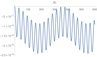
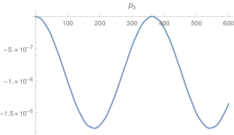
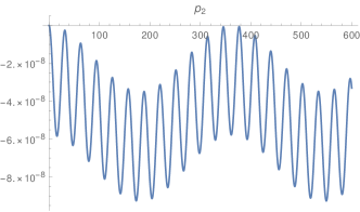
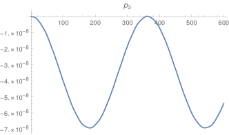
Figure 1: Time evolution over the interval $[0,\mathcal{O}(\varepsilon^{-1})]$ of the variables $p_{2}(t)$ and $p_{3}(t)$. Comparison between $r=2$ (top) and $r=3$ (bottom).

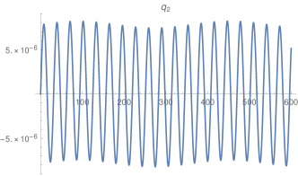
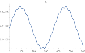
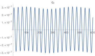
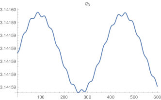
Figure 2: Time evolution over the interval $[0,\mathcal{O}(\varepsilon^{-1})]$ of the variables $q_{2}(t)$ and $q_{3}(t)$. Comparison between $r=2$ (top) and $r=3$ (bottom).

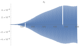
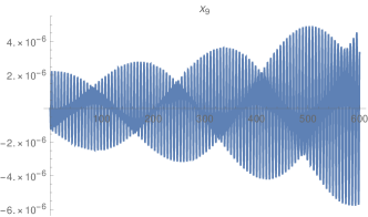
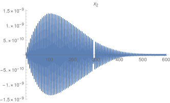
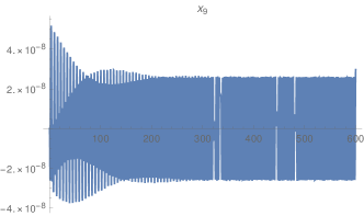
Figure 3: Time evolution over the interval $[0,600]$ of the variables $x_{2}(t)$ and $x_{9}(t)$. Comparison between $r=2$ (top) and $r=3$ (bottom).

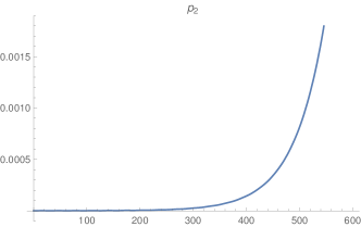
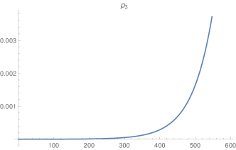
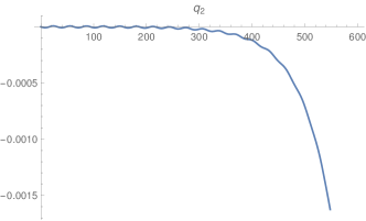
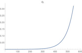
Figure 4: Time evolution over the interval $[0,\mathcal{O}(\varepsilon^{-1})]$ of the variables $p_{2}(t)$, $p_{3}(t)$ (top) and $q_{2}(t)$, $q_{3}(t)$ (bottom) for $q^{*}=(0,0)$.

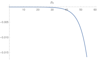
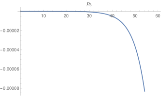
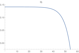
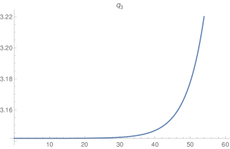
Figure 5: Time evolution over the interval $[0,\mathcal{O}(\varepsilon^{-\frac{1}{2}})]$ of the variables $p_{2}(t)$, $p_{3}(t)$ (top) and $q_{2}(t)$, $q_{3}(t)$ (bottom) for $q^{*}=(\pi,\pi)$.

4.2 Linear stability of the approximate periodic orbit

Looking at Figures 1 and 2, independently of the normalisation order considered, it is evident both the linear stability of the orbit, over the time interval according to the slowest frequency, and the effect of the two frequencies, which have a different scaling in $\varepsilon$, as illustrated in the previous section. In particular, the variables $p_{3}$ and $q_{3}$ clearly show the periodic effect mainly due to the frequency $\sqrt{3}\varepsilon$, while the variables $p_{2}$ and $q_{2}$ clearly have a faster oscillation of the order of the frequency $2\sqrt{\varepsilon}$ (actually $p_{2}$ have a quasi-periodic dynamics which exhibits both the frequencies). In a similar way, Figures 4 and 5 show the effect of instability of the approximate periodic orbit, over two different time scales. Indeed, in Figure 4 the exponentially fast separation from the approximate periodic orbit requires time of order $\mathcal{O}(\varepsilon^{-1})$, coherently with the real eigenvalues $\sqrt{3}\varepsilon$ of the $q^{*}=(0,0)$ solution. On the other hand, in Figure 5 the departure is much faster and occurs already on a time scale of order $\mathcal{O}(\varepsilon^{-\frac{1}{2}})$, coherently with the real eigenvalues $2\sqrt{\varepsilon}$ of the $q^{*}=(\pi,\pi)$ solution.

5 Conclusions

In this paper we applied an abstract result on the break down of a fully resonant torus in nearly integrable Hamiltonian system, to revisit the existence of time periodic and spatially localised solutions in dNLS lattices, such as discrete solitons or multi-pulse solitons. We considered several different dNLS models, starting from the standard one, moving to coupled dNLS chains (Zigzag or railway models) up to model with a purely nonlinear interaction. In all these cases we showed that for $\varepsilon$ small enough, i.e., in the limit of small coupling, this class of solutions are at leading order degenerate; hence a first order average is not conclusive. The normal form scheme developed in [29] and the main Theorems on existence and linear stability there included, allow to investigate, with the help of a computer algebra system, different kind of degenerate configurations, thus confirming the practical applicability of the abstract algorithm. At the same time, it allows to shed some light on a wider class of localised periodic solutions, leading to the (expected) existence of 2-dimensional resonant tori, thanks to the action of the Gauge symmetry of the dNLS models. These are special localised solutions that typically do not exist in Klein-Gordon lattices: indeed, the presence of the full Fourier spectrum of the unperturbed oscillators provides nondegenerate configurations even for a resonant modulus $M_{\omega}$ different from the $1:\text{\textendash}:1$ (see for example [15, 16, 23]). Actually, the possibility to apply the present approach to multibreathers in weakly coupled chain of oscillators is limited by the need to explicitly transform the excited oscillators to action-angle variables; this is a problem which might be overcome with special choices of the nonlinear potential, like the Morse potential, or with a preliminary dNLS normal form approximation of the nonlinear lattice (as in [18, 24]). Another example of Hamiltonian Lattice where we expect that this approach might led to interesting results is the FPU model. A recent work [5] has shown how to deal with the original FPU model in order to split the variables describing a low dimensional elliptic invariant torus from the variables describing the transversal dynamics; the same strategy might be adapted in order to study completely resonant low dimensional tori and the corresponding periodic orbits, possibly at the thermodynamic limit. Finally, a different direction of future development could be to extend the scheme in order to study the existence of degenerate quasi-periodic solutions (degenerate KAM-subtori, as in [34]), both from an abstract point of view and in terms of applications to physical models.

Acknowledgements M.S., T. P. and V. D. have been supported by the GNFM - Progetto Giovani funding “Low-dimensional Invariant Tori in FPU-like Lattices via Normal Forms” and by the MIUR-PRIN 20178CJA2B “New Frontiers of Celestial Mechanics: theory and Applications”. We all thank Vassilis Koukouloyannis for his visit to Milan in November 2019, which brought to interesting discussions on the applications here illustrated.

References

• [1] D. Bambusi, A Reversible Nekhoroshev Theorem for Persistence of Invariant Tori in Systems with Symmetry, Mathematical Physics Analysis and Geometry, 18, 1–10 (2015).
• [2] D. Bambusi, G. Gaeta, On persistence of invariant tori and a theorem by Nekhoroshev, Mathematical Physics Electronic Journal, 8, 1–13 (2002).
• [3] D. Bambusi, D. Vella, Quasi periodic breathers in Hamiltonian lattices with symmetries, Discrete & Continuous Dynamical Systems - B, 2, 389-399, 2002.
• [4] A.D. Bruno, Normalization of a Periodic Hamiltonian System, Programming and Computer Software, 46, 76–83 (2020).
• [5] C. Caracciolo, U.Locatelli, Elliptic tori in FPU non-linear chains with small number of nodes, Communications in Nonlinear Science and Numerical Simulation, 97, 105759 (2021).
• [6] J.C. Eilbeck, M. Johansson, The Discrete Nonlinear Schroedinger Equation - 20 years on, Localization and Energy Transfer in Nonlinear Systems, 44–67 (2003).
• [7] S. Flach, Conditions on the existence of localised excitations in nonlinear discrete systems, Phys. Rev. E, 50, 3134–3142 (1994).
• [8] A. Giorgilli, U. Locatelli, M. Sansottera, On the convergence of an algorithm constructing the normal form for elliptic lower dimensional tori in planetary systems, Celest Mech Dyn Astr, 119, 397–424 (2014).
• [9] A. Giorgilli, On a theorem of Lyapounov, Rend. Ist. Lombardo Acc. Sc. Lett., 146, 133–160 (2012).
• [10] D. Hennig, G.P. Tsironis, Wave transmission in nonlinear lattices, Physics Reports, 307, 333–432 (1999).
• [11] T. Kapitula, Stability of waves in perturbed Hamiltonian systems, Physica D, 156, 186–200 (2001).
• [12] T. Kapitula, P.G. Kevrekidis, Stability of waves in discrete systems, Nonlinearity, 14, 533–566 (2001).
• [13] P.G. Kevrekidis, The discrete nonlinear Schrödinger equation, Springer-Verlag, Berlin Heidelberg (2009).
• [14] P.G. Kevrekidis, Non-nearest-neighbor interactions in nonlinear dynamical lattices, Physics Letters A, 373, 3688–3693 (2009).
• [15] V. Koukouloyannis, S. Ichtiaroglou, Existence of multibreathers in chains of coupled one-dimensional Hamiltonian oscillators, Phys. Rev. E, 66, 066602 (2002).
• [16] V. Koukouloyannis, Semi-numerical method for tracking multibreathers in Klein-Gordon chains, Phys. Rev. E, 69, 046613 (2004).
• [17] B. Malomed, Nonlinearity and Discreteness: Solitons in Lattices, Emerging frontiers in Nonlinear Science, 81-110 (2020).
• [18] S. Paleari, T. Penati, An extensive resonant normal form for an arbitrary large Klein-Gordon model, Annali Matematica Pura ed Applicata, 195, 133–165 (2016).
• [19] P. Panayotaros, Continuation and bifurcations of breathers in a finite discrete NLS equation, Discrete & Continuous Dynamical Systems - S, 4, 1227–1245 (2011).
• [20] R. Parker, P.G. Kevrekidis, B. Sandstede, Existence and spectral stability of multi-pulses in discrete Hamiltonian lattice systems, Physica D, 408, 132414 (2020).
• [21] D.E. Pelinovsky, P.G. Kevrekidis, D.J. Frantzeskakis, Stability of discrete solitons in nonlinear Schrödinger lattices, Physica D, 212, 1–19 (2005).
• [22] D.E. Pelinovsky, P.G. Kevrekidis, D.J. Frantzeskakis, Persistence and stability of discrete vortices in nonlinear Schrödinger lattices. Physica D, 212, 20–53 (2005).
• [23] D. Pelinovsky, A. Sakovich, Multi-site breathers in Klein-Gordon lattices: stability, resonances and bifurcations, Nonlinearity, 25, 3423–3451 (2012).
• [24] D. Pelinovsky, T. Penati, S. Paleari, Approximation of small-amplitude weakly coupled oscillators by discrete nonlinear Schrödinger equations, Reviews in Mathematical Physics, 28, 1650015 (2016).
• [25] T. Penati, M. Sansottera, S. Paleari, V. Koukouloyannis, P.G. Kevrekidis, On the nonexistence of degenerate phase-shift discrete solitons in a dNLS nonlocal lattice, Physica D, 370, 1–13 (2018).
• [26] T. Penati, V. Koukouloyannis, M. Sansottera, P.G. Kevrekidis, S. Paleari, On thenonexistence of degenerate phase-shift multibreathers in Klein-Gordon models with interactions beyond nearest neighbors, Physica D, 398, 92–114 (2019).
• [27] T. Penati, M. Sansottera, V. Danesi, On the continuation of degenerate periodic orbits via normal form: full dimensional resonant tori, Communications in Nonlinear Science and Numerical Simulation, 61, 198–224 (2018).
• [28] P. Rosenau, S. Schochet, Compact and almost compact breathers: a bridge between an anharmonic lattice and its continuum limit, Chaos: An Interdisciplinary Journal of Nonlinear Science 15, 015111 (2005).
• [29] M. Sansottera, V. Danesi, T. Penati, S.Paleari, On the continuation of degenerate periodic orbits via normal form: lower dimensional resonant tori, Communications in Nonlinear Science and Numerical Simulation, 90, 105360 (2020).
• [30] M. Sansottera, A.-S. Libert, Resonant Laplace-Lagrange theory for extrasolar systems in mean-motion resonance, Celest Mech Dyn Astr, 131, 38 (2019).
• [31] M. Sansottera, U. Locatelli, A. Giorgilli, A semi-analytic algorithm for constructing lower dimensional elliptic tori in planetary systems, Celest Mech Dyn Astr, 111, 337–361 (2011).
• [32] S. Paleari, T. Penati Hamiltonian Lattice Dynamics Editorial for the Special Issue “Hamiltonian Lattice Dynamics”, Mathematics in Engineering, 1 (4):881-887, 2019.
• [33] T. Penati, V. Danesi, S.Paleari, Low dimensional completely resonant tori in Hamiltonian Lattices and a Theorem of Poincaré, Mathematics in Engineering 3(4), 1–20 (2021).
• [34] D.V. Treshchëv, The mechanism of destruction of resonant tori of Hamiltonian systems, Math. USSR Sb., 68, 181–203 (1991).
• [35] W.-X. Qin, X. Xiao, Homoclinic orbits and localized solutions in nonlinear Schrödinger lattices, Nonlinearity, 20, 2305–2317 (2007).