Vacuum instability due to the creation of neutral Fermion with anomalous magnetic moment by magnetic-field inhomogeneities

Abstract

We study neutral Fermions pair creation with anomalous magnetic moment from the vacuum by time-independent magnetic-field inhomogeneity as an external background. We show that the problem is technically reduced to the problem of charged-particle creation by an electric step, for which the nonperturbative formulation of strong-field QED is used. We consider a magnetic step given by an analytic function and whose inhomogeneity may vary from a “gradual” to a “sharp” field configuration. We obtain corresponding exact solutions of the Dirac-Pauli equation with this field and calculate pertinent quantities characterizing vacuum instability, such as the differential mean number and flux density of pairs created from the vacuum, vacuum fluxes of energy and magnetic moment. We show that the vacuum flux in one direction is formed from fluxes of particles and antiparticles of equal intensity and with the same magnetic moments parallel to the external field. Backreaction to the vacuum fluxes leads to a smoothing of the magnetic-field inhomogeneity. We also estimate critical magnetic field intensities, near which the phenomenon could be observed.

1 Introduction

The violation of vacuum stability stimulated by external electromagnetic fields is commonly associated with the possibility of such backgrounds producing work on virtual pairs of particles and antiparticles. The most well-known examples are electric-like fields, as they produce work on charged particles and are able to tear apart electron/positron pairs from the vacuum if the field amplitudes approach the so-called Schwinger critical value $E_{\mathrm{c}}=m^{2}c^{3}/e\hslash\approx 1.3\times 10^{16}\,\mathrm{V}/\mathrm{cm}$ [1]. The phenomenon has been a subject of intense investigation since the seminal works of Klein [2], Sauter [3, 4], Heisenberg and Euler [5], and Schwinger [1]. An extensive discussion about the origin of the effect, theoretical foundations, and experimental aspects can be found in some reviews and monographs; see e.g. [6, 7, 8, 9, 10, 11, 12, 13, 14, 15] and references therein.

Following the above interpretation, one may ask oneself about the possibility that inhomogeneous macroscopic magnetic fields which, contrary to homogeneous magnetic fields, produce a work on particles with a magnetic moment, may create pairs from the vacuum. The answer to this question is affirmative, provided the particles are neutral and have an anomalous magnetic moment. Bearing in mind, first of all, very strong magnetic fields observed in astrophysics, we can assume that this type of fields is practically time-independent and steplike, that is, their gradient is always positive. It must be said that the works available in the literature on calculating such an effect, using sometimes inconsistent heuristic approaches, often contradict each other [16, 17, 18, 19]. In this regard, in work [20], it was shown that the problem could be formally reduced to the calculation of charged particle creation from the vacuum by stationary inhomogeneous electric fields of constant direction (the so-called electric step potential gives this field). In particular, it was shown that we are technically dealing with the calculation of an effect similar to the well-known Klein effect, see Refs. [2, 3, 4]. We recall that study of the effect began early in the framework of relativistic quantum mechanics, see Ref. [21] for a review; its consistent nonperturbative description within QED was given by Gavrilov and Gitman, in Refs. [22, 23].

At present, there exist two types of particles enjoying the properties mentioned above: the neutron and the neutrino. According to experimental data, neutrons have a magnetic moment $\mu_{N}\approx-1.04187563(25)\times 10^{-3}\mu_{\mathrm{B}}$ [24], where $\mu_{\mathrm{B}}$ is the Bohr magneton. As for neutrinos, there is not a general consensus because of the different types of neutrinos, mechanism under which neutrinos acquires magnetic moment, specific models, etc. Presently, experimental constraints range from $\mu_{\nu_{\tau}}<3.9\times 10^{-7}\mu_{\mathrm{B}}$ (for the tau neutrino) [25] until $\mu_{\nu_{e}}<2.9\times 10^{-11}\mu_{\mathrm{B}}$ (for the electron neutrino) [26]. Moreover, stringent constraints obtained from astrophysical observations [27, 28, 29, 30, 31, 32] indicate that $\mu_{\nu}<\left(2.6-4.5\right)\times 10^{-12}\mu_{\mathrm{B}}$ while lower upper bounds, predicted by effective theories above the electroweak scale, suggest that $\mu_{\nu}<10^{-14}\mu_{\mathrm{B}}$ [33]. It is important to point out that for some theories beyond the Standard Model (SM) [34], it was reported that the magnetic moment for the neutrinos lie within the range $\left(10^{-12}-10^{-14}\right)\mu_{\mathrm{B}}$. For a more extensive discussion concerning experimental aspects and theoretical predictions for neutrinos’ electromagnetic properties, see e.g. the reviews [35, 36, 37, 38, 39] and references therein.

Vacuum instability effects due to inhomogeneous magnetic fields may be relevant to studies on dark matter. One of the reasons concerns the existence of sterile neutrinos, which may constitute dark matter and also couple to external magnetic fields through their electromagnetic properties. Presently, it is known that light sterile neutrinos appear in the low-energy effective theory in most extensions of the SM and, in principle, can have any mass, particularly in the range of $1\,\mathrm{eV}$. Sterile neutrinos with masses of several $\mathrm{keV}$ can account for cosmological dark matter, see e.g. Refs. [40, 41] for a recent review, and references therein. It is possible that due to some new physics, the neutrino magnetic moment is big. Various observational constraints on the magnetic moment $\mu$ of a dark matter particle for masses $M$ in the range $1\,\mathrm{keV}$ to $100\,\mathrm{MeV}$ have been considered in Refs. [42, 43]. The strongest limits on $\mu$ emerge at the lightest mass scales. For example, if $M=m_{e}/10$, then $\left|\mu\right|<3.4\times 10^{-5}\mu_{B}$ due to precision electroweak measurements.

Apart from neutral particles, it is important to mention that charged particles can be created by inhomogeneous magnetic fields in de Sitter spacetimes [44, 45, 46]. In Refs. [44, 45] for instance, the authors calculated transition amplitudes and probabilities of charged pair production by the magnetic field of a magnetic dipole as an external background in de Sitter spacetime perturbatively and shown that the corresponding probabilities are nontrivial. In Ref. [46], the consideration was further extended to the case where an external Coulomb field creates charged particles. Theoretically, it is also known that pairs of particles and antiparticles having a magnetic charge can be created by a constant and homogeneous magnetic field [47, 48]. This matter has gained considerable attention lately due to the possibility of monopole-antimonopole and axion-like particle pair production in the early Universe [49, 50, 51, 52] and during heavy-ion collisions [53, 54, 55], especially with the design of recent experiments aimed at detecting magnetic monopoles in the Large Hadron Collider (LHC); e.g. [56, 57, 58] (see also Ref. [59] for a review). In particular, the mechanism of monopole-antimonopole pair production provides an explanation for the dissipation of primordial magnetic fields consistent with gamma ray observations of intergalactic magnetic fields [60, 61, 62]. It has been discussed that even heavy monopoles (with masses $\sim 10^{16}\,\mathrm{GeV}$) could be pair produced in the early Universe [49]. Besides the aforementioned types of particles and external backgrounds, it should be noted that neutrino/antineutrino ($\nu\bar{\nu}$) pairs may also be created from the vacuum by dense matters as external backgrounds. For example, it was reported some years ago that $\nu\bar{\nu}$ pairs can be created in Neutron stars [63, 64] due to the interaction with the background matter. In these works, the authors considered time-independent matter densities and calculated $\nu\bar{\nu}$ pair production rate in analogy with Schwinger’s result for electron-positron pair production by a constant electric field [1]. It was also reported that $\nu\bar{\nu}$ pairs can also be created due to a coherent interaction with a dense medium [65]. Some years later, $\nu\bar{\nu}$ pair production rates for time-dependent matter densities were calculated nonperturbatively through semiclassical methods in Ref. [66] and perturbatively in Ref. [67], using the $S$-matrix formalism. More recently, some of us [68] considered a consistent nonperturbative formulation for calculating $\nu\bar{\nu}$ pair creation from the vacuum by a time-dependent background matter. It was also demonstrated in Ref. [69] that $\nu\bar{\nu}$ pairs could be created from the vacuum by an accelerated matter due to the neutrino electroweak interaction with background Fermions.

Understanding the mechanism responsible for neutral Fermion pair production by intense magnetic fields may be particularly important to comprehend the physics of highly magnetized astrophysical objects and events occurring in the Universe. For example, it was reported a few years ago [70, 71, 72], that magnetic fields of the order of $10^{16}-10^{18}\,\mathrm{G}$ could be generated during a supernova explosion or in the vicinity of magnetars. Moreover, ultra-intense magnetic fields (of order up to $10^{20}\ \mathrm{G}$) can be produced at the core of compact magnetars [73]. Based on experimental values for the neutron mass and its magnetic moment [24], it is possible that such objects can produce pairs of neutrons/antineutrons, and it may affect their inner dynamics. Another important aspect of the present study concerns the possibility of inspecting conditions for neutrino pair production based on predictions for the neutrinos magnetic moment supplied by the SM $\mu_{\nu}\approx 3.2\times 10^{-19}\mu_{\mathrm{B}}\times\left(m_{\nu}/1\,\mathrm{eV}\right)$ [35, 38]. Considering an acceptable range of values to neutrinos masses, say $1\,\mathrm{eV}-10^{-2}\,\mathrm{eV}$, we discuss below that neutrinos with such small magnetic moments can be created only by inhomogeneous magnetic fields several orders above the astronomical scale. The situation is very different for neutrinos with larger magnetic moments, which could be already created from the vacuum by magnetic fields of order $10^{16}\,\mathrm{G}$. Thus, neutrino pair production by intense magnetic-field inhomogeneity may indirectly indicate that the SM must be extended in order to account for larger magnetic moments, possibly near the experimental reach.

The mechanism discussed in this work corresponds to the most fundamental process driven by the interaction between neutral Fermions with electromagnetic backgrounds, namely the creation of neutral Fermion pairs with anomalous magnetic moment from the vacuum by an inhomogeneous external magnetic field. The process in consideration is particularly different from neutrino pair production by an electron in a constant magnetic field, in which neutrino/antineutrino pairs are created as a decay process of the initial electron stimulated by the magnetic field; see e.g. Ref. [38] and references therein. It was demonstrated in [20] that a quantization in terms of neutral particles and antiparticles is possible in terms of the states with well-defined spin polarization. In this case, the problem can be technically reduced to the problem of charged-particle creation by electric fields given by step potentials (in short, electric steps) for which a nonperturbative formulation in QED [22, 23] can be used. This formulation is based on the possibility of finding exact solutions to the Dirac-Pauli equation with steplike magnetic fields. As an example, neutral Fermion creation from the vacuum by a linearly growing magnetic field was considered in Ref. [20]. In the present article, we develop the technique proposed in Ref. [20] taking into account recent theoretical constructions [22, 23]. Based on these developments, we study neutral Fermion pair production from the vacuum by the magnetic step given by an analytic function that enables studying the role of the field inhomogeneity on pair production. In Sec. 2 we demonstrate how to reduce the problem under consideration to the problem of charged-particle creation by an electric step. In Sec. 3, we describe the field in consideration and construct corresponding in- and out-solutions of the Dirac-Pauli equation with this field. With the aid of these solutions, we find differential and total quantities characterizing vacuum instability. In Secs. 4 and 5, we present these quantities and scrutinize their behavior when the field varies “gradually” or “sharply” along the inhomogeneity direction. Numerical estimates to the critical field are given. In Sec. 6, we find vacuum fluxes of energy and the magnetic moment produced by the magnetic-field inhomogeneity. Sec. 7 is devoted to the concluding remarks. In this work we consider the four-dimensional Minkowski spacetime, parameterized by coordinates $X=\left(X^{\mu}\,,\ \mu=0,i\right)=\left(t,\mathbf{r}\right)$, $t=X^{0}$, $\mathbf{r}=X^{i}=\left(x,y,z\right)$, $i=1,2,3$, and metric tensor $\eta_{\mu\nu}=\mathrm{diag}\left(+1,-1,-1,-1\right)$. We also employ natural units, in which $\hslash=1=c$.

2 Solutions of the Dirac-Pauli equation with well-defined spin polarization

In this section we present general considerations on the Dirac-Pauli equation with inhomogeneous magnetic fields. In particular, we discuss the spinor structure of solutions and their asymptotic properties at specific remote distances. Such properties are important to correctly classify solutions and to define quantities characterizing vacuum instability, as discussed in Sec. 4.

The motion of a relativistic spin $1/2$ neutral particle with anomalous magnetic moment $\mu$, mass $m$, in external electromagnetic fields is described by the relativistic wave equation

$$\left(i\gamma^{\mu}\partial_{\mu}-m-\frac{1}{2}\mu\sigma^{\mu\nu}F_{\mu\nu}\right)\psi\left(X\right)=0\,,$$ (1)

which is conventionally called the Dirac-Pauli (DP) equation [74]. Here $\psi\left(X\right)$ is a four spinor, $\gamma^{\mu}=\left(\gamma^{0},\boldsymbol{\gamma}\right)$ are Dirac matrices, $\sigma^{\mu\nu}=\left(i/2\right)\left[\gamma^{\mu},\gamma^{\nu}\right]_{-}$, $F_{\mu\nu}=\partial_{\mu}A_{\nu}-\partial_{\nu}A_{\mu}$ is the electromagnetic field strength tensor, and $\mu$ should be understood as the algebraic value of the magnetic moment (e.g., $\mu=-\left|\mu_{N}\right|$ for a neutron). In what follows we consider external fields of a specific type, corresponding to a time-independent magnetic field oriented along the positive direction of the $z$-axis, inhomogeneous along the $y$-direction, $\mathbf{B}\left(\mathbf{r}\right)=\left(0,0,B_{z}\left(y\right)\right)$, and homogeneous at remote distances, $B_{z}\left(\pm\infty\right)=\mathrm{const}$. Moreover, it is assumed that its gradient is always positive $\partial_{y}B\left(y\right)\geq 0$,$\ \forall\,y\in\left(-\infty,+\infty\right)$, meaning that $B_{z}\left(+\infty\right)>B_{z}\left(-\infty\right)$ and that the field is genuinely a step. We conveniently refer to fields of this type as steplike magnetic fields or simply as magnetic steps.

The general method for solving the DP equation (1) with steplike magnetic fields was presented before by two of us in Ref. [20]. We recall some properties of the DP equation with such fields and present new details that simplify the spinor structure of the solutions. In the Schrödinger form, the DP equation (1) reads

$$i\partial_{t}\psi\left(X\right)=\hat{H}\psi\left(X\right)\,,\ \ \hat{H}=\gamma^{0}\left(\gamma^{3}\hat{p}_{z}+\Sigma_{z}\hat{\Pi}_{z}\right)\,.$$ (2)

Here $\Sigma_{z}=i\gamma^{1}\gamma^{2}$ and

$$\hat{\Pi}_{z}=\Sigma_{z}\left(\boldsymbol{\gamma}\mathbf{\hat{p}}_{\perp}+m\right)-\mathbb{I}\mu B_{z}\left(y\right)\,,$$ (3)

is an integral of motion spin-operator, $\left[\hat{\Pi}_{z},\hat{H}\right]_{-}=0$. The subscript “$\perp$” labels quantities perpendicular to the field, e.g. $\mathbf{\hat{p}}_{\perp}=\left(\hat{p}_{x},\hat{p}_{y}\right)$, and $\mathbb{I}$ denotes the $4\times 4$ identity matrix. Since the operators $\hat{p}_{0}$, $\hat{p}_{x}$, and $\hat{p}_{z}$ are compatible with the Hamiltonian (and also with $\hat{\Pi}_{z}$), the DP spinor admits the general form $\psi_{n}\left(X\right)=\exp\left(-ip_{0}t+ip_{x}x+ip_{z}z\right)\psi_{n}\left(y\right)$, where $\psi_{n}\left(y\right)$ depends exclusively on $y$ and obeys the eigenvalue equation:

$$\hat{\Pi}_{z}\psi_{n}\left(X\right)=e^{-ip_{0}t+ip_{x}x+ip_{z}z}\Pi_{z}\psi_{n}\left(y\right)\,,\ \ \Pi_{z}\psi_{n}\left(y\right)=s\omega\psi_{n}\left(y\right)\,,\ \ s=\pm 1\,,$$

$$\Pi_{z}=\hat{\pi}_{z}-\mathbb{I}\mu B_{z}\left(y\right)\,,\ \ \hat{\pi}_{z}=\Sigma_{z}\left(\gamma^{1}p_{x}+\gamma^{2}\hat{p}_{y}+m\right)\,,$$ (4)

By acting the squared Hamiltonian operator (2) onto $\psi_{n}\left(X\right)$, we observe that the total particle’s energy $p_{0}$, longitudinal momentum $p_{z}$, and $\omega$ are interrelated, $p_{0}^{2}=\omega^{2}+p_{z}^{2}\rightarrow p_{0}=\omega\sqrt{1+p_{z}^{2}/\omega^{2}}$, $\mathrm{sgn}\left(p_{0}\right)=\mathrm{sgn}\left(\omega\right)$. This relation indicates that $\omega$ is the transverse part of the total energy. Thanks to this identity, we may introduce an additional operator

$$\hat{R}=\hat{H}\hat{\Pi}_{z}^{-1}\left[\mathbb{I}+\left(\hat{p}_{z}\hat{\Pi}_{z}^{-1}\right)^{2}\right]^{-1/2}\,,$$ (5)

which is also an integral of motion and commutes with all previous operators. In particular, this operator implies that $\psi_{n}\left(y\right)$ also obeys the eigenvalue equation

$$\hat{R}\psi_{n}\left(X\right)=e^{-ip_{0}t+ip_{x}x+ip_{z}z}R\psi_{n}\left(y\right)\,,\ \ R\psi_{n}\left(y\right)=s\psi_{n}\left(y\right)\,,$$

$$R=\Upsilon\gamma^{0}\left(\Sigma_{z}+\frac{sp_{z}}{\omega}\gamma^{3}\right)\,,\ \ \Upsilon=\frac{1}{\sqrt{1+p_{z}^{2}/\omega^{2}}}\,.$$ (6)

As a result, we select $\hat{p}_{x}$, $\hat{p}_{z}$, $\hat{\Pi}_{z}$, $\hat{R}$ as the complete set of commuting operators, whose eigenvalues are $n=\left(p_{x},p_{z},\omega,s\right)$.

The set of equations (4) and (6) are simultaneously satisfied choosing $\psi_{n}\left(y\right)$ in the form

$$\psi_{n}\left(y\right)=\left(\mathbb{I}+sR\right)\left[\hat{\pi}_{z}+\mathbb{I}\left(\mu B_{z}\left(y\right)+s\omega\right)\right]\varphi_{n,\chi}\left(y\right)\upsilon_{\kappa}^{\left(\chi\right)}\,,$$ (7)

where $\varphi_{n,\chi}\left(y\right)$ are functions while $\upsilon_{\kappa}^{\left(\chi\right)}$ belongs to a set of four constant spinors, satisfying the eigenvalue equations

$$i\gamma^{1}\upsilon_{\kappa}^{\left(\chi\right)}=\chi\upsilon_{\kappa}^{\left(\chi\right)}\,,\ \ \gamma^{0}\gamma^{2}\upsilon_{\kappa}^{\left(\chi\right)}=\kappa\upsilon_{\kappa}^{\left(\chi\right)}\,,\ \ \chi=\pm 1\,,\ \ \kappa=\pm 1\,,$$ (8)

and the orthonormality conditions $\upsilon_{\kappa^{\prime}}^{\left(\chi^{\prime}\right)\dagger}\upsilon_{\kappa}^{\left(\chi\right)}=\delta_{\chi^{\prime}\chi}\delta_{\kappa^{\prime}\kappa}$. Substituting the spinor (7) into (4) one finds that the scalar functions $\varphi_{n,\chi}\left(y\right)$ are solutions of the second-order ordinary differential equation

$$\left\{-\frac{d^{2}}{dy^{2}}-\left[s\omega+\mu B_{z}\left(y\right)\right]^{2}+\pi_{x}^{2}+i\mu\chi B_{z}^{\prime}\left(y\right)\right\}\varphi_{n,\chi}\left(y\right)=0\,,\ \ \pi_{x}^{2}=m^{2}+p_{x}^{2}\,.$$ (9)

Although the separation of degrees-of-freedom given by Eq. (7) simplifies the structure of the solutions, it is important to point out that none of the operators listed in (8) are integrals of motion. Thus, it is possible to select any spinor of the basis $\upsilon_{\kappa}^{\left(\chi\right)}$ to study pair creation. To keep expressions as general as possible, we leave this choice arbitrary in all calculations below.

At this point, it is worth discussing some general features of neutral Fermions in the external field and properties of the solutions. Because of the spectrum of the spin operator $\hat{R}$, there are two species of neutral Fermions differing by the value of $s$–one species for which $s=+1$ and another for which $s=-1$. Consequently, the potential energy of a neutral Fermion in this field is given by $U_{s}\left(y\right)=sU\left(y\right)$, where $U\left(y\right)=-\mu B_{z}\left(y\right)$. To facilitate subsequent discussions, it is convenient to select a fixed sign for particle magnetic moment. Thus, from now on, we choose a Fermion with a negative magnetic moment as the main particle, $\mu=-\left|\mu\right|$. Since the external field increases monotonically with $y$ (its gradient is positive, as stated before), the maximum potential energy that may be experienced by the Fermion is determined by the magnitude of the step

$$\mathbb{U}\equiv U_{\mathrm{R}}-U_{\mathrm{L}}>0\,,$$ (10)

which is essentially the difference between the asymptotic values $U_{\mathrm{R}}=U\left(+\infty\right)$, $U_{\mathrm{L}}=U\left(-\infty\right)$ and is positive, by definition. Thus, for Fermions with $s=+1$, the magnitude of the potential step is $\mathbb{U}=U_{+1}\left(\mathrm{R}\right)-U_{+1}\left(\mathrm{L}\right)$ while for Fermions with $s=-1$ it is $\mathbb{U}=U_{-1}\left(\mathrm{L}\right)-U_{-1}\left(\mathrm{R}\right)$, where $U_{s}\left(\mathrm{L/R}\right)=sU_{\mathrm{L/R}}$. At remote distances–where the field can be considered as homogeneous and no longer accelerates particles–the term proportional to $\chi$ in Eq. (9) is absent. Therefore, solutions of Eq. (9) intrinsically have well-defined left $\ {}_{\zeta}\varphi_{n,\chi}\left(y\right)$ and right $\ {}^{\zeta}\varphi_{n,\chi}\left(y\right)$ asymptotic forms

$$\ {}_{\zeta}\varphi_{n,\chi}\left(y\right) = \ {}_{\zeta}\mathcal{N}\exp\left(i\zeta\left|p^{\mathrm{L}}\right|y\right)\,,\ \ \zeta=\mathrm{sgn}\left(p^{\mathrm{L}}\right)\,,\ \ y\rightarrow-\infty\,,$$

$$\ {}^{\zeta}\varphi_{n,\chi}\left(y\right) = \ {}^{\zeta}\mathcal{N}\exp\left(i\zeta\left|p^{\mathrm{R}}\right|y\right)\,,\ \ \zeta=\mathrm{sgn}\left(p^{\mathrm{R}}\right)\,,\ \ y\rightarrow+\infty\,,$$ (11)

in which $\ {}_{\zeta}\mathcal{N}$, $\ {}^{\zeta}\mathcal{N}$ are normalization constants, $\left|p^{\mathrm{L/R}}\right|$ are $y$-components of Fermions momenta at corresponding remote regions,

$$\left|p^{\mathrm{L/R}}\right|=\sqrt{\left[s\pi_{s}\left(\mathrm{L/R}\right)\right]^{2}-\pi_{x}^{2}}\,,\ \ \pi_{s}\left(\mathrm{L/R}\right)=\omega-sU_{\mathrm{L/R}}\,,$$ (12)

and $\pi_{s}\left(\mathrm{L/R}\right)$ are their transverse kinetic energies at remote areas. Correspondingly, we may introduce the asymptotically-left $\ {}_{\zeta}\psi_{n}\left(X\right)=\exp\left(-ip_{0}t+ip_{x}x+ip_{z}z\right)\ _{\zeta}\psi_{n}\left(y\right)$ and the asymptotically-right ${}^{\zeta}\psi_{n}\left(X\right)=\exp\left(-ip_{0}t+ip_{x}x+ip_{z}z\right)\ ^{\zeta}\psi_{n}\left(y\right)$ sets of DP spinors

$$\ {}_{\zeta}\psi_{n}\left(y\right) = \ {}_{\zeta}\mathcal{N}e^{i\zeta\left|p^{\mathrm{L}}\right|y}\left(\mathbb{I}+sR\right)\left[\Sigma_{z}\left(\gamma^{1}p_{x}+m\right)+\mathbb{I}\left(s\pi_{s}\left(\mathrm{L}\right)-\chi\zeta\left|p^{\mathrm{L}}\right|\right)\right]\upsilon_{\kappa}^{\left(\chi\right)}\,,\ \ y\rightarrow-\infty\,,$$

$$\ {}^{\zeta}\psi_{n}\left(y\right) = \ {}^{\zeta}\mathcal{N}e^{i\zeta\left|p^{\mathrm{R}}\right|y}\left(\mathbb{I}+sR\right)\left[\Sigma_{z}\left(\gamma^{1}p_{x}+m\right)+\mathbb{I}\left(s\pi_{s}\left(\mathrm{R}\right)-\chi\zeta\left|p^{\mathrm{R}}\right|\right)\right]\upsilon_{\kappa}^{\left(\chi\right)}\,,\ \ y\rightarrow+\infty\,,$$ (13)

which, in turn, obey the eigenvalue equations

$$\hat{p}_{y}\ {}_{\zeta}\psi_{n}\left(X\right)=\zeta\left|p^{\mathrm{L}}\right|\ _{\zeta}\psi_{n}\left(X\right)\,,\ \ \hat{h}_{\perp}^{\mathrm{kin}}\ {}_{\zeta}\psi_{n}\left(X\right)=s\pi_{s}\left(\mathrm{L}\right)\ _{\zeta}\psi_{n}\left(X\right)\,,\ \ y\rightarrow-\infty\,,$$

$$\hat{p}_{y}\ ^{\zeta}\psi_{n}\left(X\right)=\zeta\left|p^{\mathrm{R}}\right|\ ^{\zeta}\psi_{n}\left(X\right)\,,\ \ \hat{h}_{\perp}^{\mathrm{kin}}\ {}^{\zeta}\psi_{n}\left(X\right)=s\pi_{s}\left(\mathrm{R}\right)\ ^{\zeta}\psi_{n}\left(X\right)\,,\ \ y\rightarrow+\infty\,,$$ (14)

where $\hat{h}_{\perp}^{\mathrm{kin}}=\hat{\Pi}_{z}-\mathbb{I}\left|\mu\right|B_{z}\left(y\right)$ is the one-particle transverse kinetic energy operator. It is important to emphasize both sets of solutions exist provided the quantum numbers $n$ obey the conditions

$$\left[s\pi_{s}\left(\mathrm{L/R}\right)\right]^{2}>\pi_{x}^{2}\,.$$ (15)

These inequalities ensure the nontriviality of DP spinors with real asymptotic momenta $p^{\mathrm{L}}$ and $p^{\mathrm{R}}$ in remote areas and impart consequences to the quantization of the theory, as shall be discussed below.

At last it should be noted that if the field is homogeneous, then the left and right asymptotic potentials coincide $U_{\mathrm{R}}=U_{\mathrm{L}}\equiv U$ and the step is trivial, $\mathbb{U}=0$. As a result, there is no distinction between the asymptotic momenta $\left|p^{\mathrm{L}}\right|=\left|p^{\mathrm{R}}\right|=p_{y}=\sqrt{\left(\omega-sU\right)^{2}-\pi_{x}^{2}}$ and the transverse kinetic energy remains the same throughout the space, $\pi_{s}\left(\mathrm{L}\right)=\pi_{s}\left(\mathrm{R}\right)\equiv\omega_{0}=\omega-sU=\pm\sqrt{m^{2}+\mathbf{p}_{\perp}^{2}}$. In a complete absence of external fields, $B_{z}\left(y\right)=0\rightarrow U=0$, the transverse kinetic energy $\omega_{0}$ fully coincides with the total transverse energy, $\omega_{0}=\omega=\pm\sqrt{m^{2}+\mathbf{p}_{\perp}^{2}}$.

It should be noted that the time independence of the magnetic field under consideration is an idealization. Physically, it is meaningful to believe that the field inhomogeneity was switched on sufficiently fast before instant $t_{\mathrm{in}}$. By this time, it had time to spread to the whole area under consideration and then acted as a constant field during a large time $T$. It is supposed that one can ignore effects of its switching on and off. This is a kind of regularization, which could, under certain conditions, be replaced by periodic boundary conditions in $t$, see Refs. [22, 23] for details. Therefore, it is convenient to use the inner product on the time-like hyperplane $y=\mathrm{const}$, which has the form

$$\left(\psi,\psi^{\prime}\right)_{y}=\int dtdxdz\psi^{\dagger}\left(X\right)\gamma^{0}\gamma^{2}\psi^{\prime}\left(X\right)\,,$$ (16)

after imposing specific normalization conditions. We assume that all processes take place in a macroscopically large space-time box, of volume $TV_{y}$, $V_{y}=L_{x}L_{z}$, and impose periodic boundary conditions upon DP spinors in the variables $t$, $x$, $z$ at the boundaries. Thus, the integrals in (16) are calculated from $\left(-T/2,-L_{x}/2,-L_{z}/2\right)$ to $\left(+T/2,+L_{x}/2,+L_{z}/2\right)$ and the limits $\left(T,L_{x},L_{z}\right)\rightarrow\infty$ are taken at the end of calculations. The time $T$ can be interpreted as a time of observation of the evolution of the system under consideration. Under these conditions, the inner product is $y$-independent and we may impose the normalization conditions

$$\left(\ {}_{\zeta^{\prime}}\psi_{n^{\prime}},\ _{\zeta}\psi_{n}\right)_{y}=\zeta\eta_{\mathrm{L}}\delta_{n^{\prime}n}\delta_{\zeta^{\prime}\zeta}\,,\ \ \left(\ {}^{\zeta^{\prime}}\psi_{n^{\prime}},\ ^{\zeta}\psi_{n}\right)_{y}=\zeta\eta_{\mathrm{R}}\delta_{n^{\prime}n}\delta_{\zeta^{\prime}\zeta}\,,\ \ \eta_{\mathrm{L/R}}=\mathrm{sgn}\left[\pi_{s}\left(\mathrm{L/R}\right)\right]\,.$$ (17)

Considering that the “left” and “right” sets of DP spinors are orthonormal and complete, we may decompose one set into another with the help of specific coefficients

$$\eta_{\mathrm{L}}\ ^{\zeta}\psi_{n}\left(X\right) = g\left({}_{+}|^{\zeta}\right)\ _{+}\psi_{n}\left(X\right)-g\left({}_{-}|^{\zeta}\right)\ _{-}\psi_{n}\left(X\right)\,,$$

$$\eta_{\mathrm{R}}\ {}_{\zeta}\psi_{n}\left(X\right) = g\left({}^{+}|_{\zeta}\right)\ ^{+}\psi_{n}\left(X\right)-g\left({}^{-}|_{\zeta}\right)\ ^{-}\psi_{n}\left(X\right)\,,$$ (18)

which, by definition, are inner products between different sets of DP spinors

$$\left(\ {}_{\zeta}\psi_{n},\ ^{\zeta^{\prime}}\psi_{n^{\prime}}\right)_{y}=\delta_{nn^{\prime}}g\left({}_{\zeta}|^{\zeta^{\prime}}\right)=\delta_{nn^{\prime}}g\left({}^{\zeta^{\prime}}|_{\zeta}\right)^{\ast}\,.$$ (19)

Substituting the identities (18) into the normalization conditions (17) supply us with two important identities

$$\sum_{\zeta^{\prime\prime}=\pm}\zeta^{\prime\prime}g\left({}^{\zeta^{\prime}}|_{\zeta^{\prime\prime}}\right)g\left({}_{\zeta^{\prime\prime}}|^{\zeta}\right)=\zeta\eta_{\mathrm{L}}\eta_{\mathrm{R}}\delta_{\zeta^{\prime}\zeta}=\sum_{\zeta^{\prime\prime}=\pm}\zeta^{\prime\prime}g\left({}_{\zeta^{\prime}}|^{\zeta^{\prime\prime}}\right)g\left({}^{\zeta^{\prime\prime}}|_{\zeta}\right)\,,$$ (20)

from which we may derive a number of supplementary identities, for example $\left|g\left({}_{+}|^{-}\right)\right|^{2}=\left|g\left({}_{-}|^{+}\right)\right|^{2}$, $\left|g\left({}_{+}|^{+}\right)\right|^{2}=\left|g\left({}_{-}|^{-}\right)\right|^{2}$, and $\left|g\left({}_{+}|^{+}\right)\right|^{2}-\left|g\left({}_{+}|^{-}\right)\right|^{2}=\eta_{\mathrm{L}}\eta_{\mathrm{R}}$.

The above-presented plane waves can form wave packets in a given asymptotic region. In this case, the problem can be technically reduced to the problem of charged-particle creation by an electric step [22, 23]. It allows to quantize the DP field operator in the framework of QED with external backgrounds. Based on this quantization, it is possible to calculate all quantities characterizing vacuum instability by steplike magnetic fields, as discussed in Sec. 4.

3 Time-independent Sauter-like magnetic step

To explicitly calculate neutral Fermion pair production, we consider the following external field

$$B_{z}\left(y\right)=\varrho B^{\prime}\tanh\left(y/\varrho\right)\,,\ \ B^{\prime}>0\,,\ \ \varrho>0\,,$$ (21)

which enjoys the properties discussed before and enables us to solve the DP equation exactly. More precisely, the field under consideration is homogeneous at remote distances, $B_{z}\left(\pm\infty\right)=\pm\varrho B^{\prime}=\mathrm{const.}$, and its gradient is always positive $\partial_{y}B_{z}\left(y\right)=B^{\prime}\cosh^{-2}\left(y/\varrho\right)\geq 0$; in particular, $\mathbb{U}=2\varrho\left|\mu\right|B^{\prime}$ for this field. The amplitude $B^{\prime}$ and the “inhomogeneity length” $\varrho$ describe, respectively, the “slope” of the field with respect to the $y$-axis and how “rectilinear” it is in the neighborhood of the origin. Thus, the larger $B^{\prime}$ and $\varrho$, the more “steep” and the more “rectilinear” the pattern of (21) near the origin. For illustrative purposes, we present in Fig. 1 the magnetic step (21) as a function of $y$, $\varrho$, and $B^{\prime}$. It should be noted that the field (21) shares the same functional form as the time-independent scalar electric potential originally considered by F. Sauter in [4], who first solved the Dirac equation with this field.

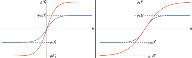
Figure 1: Magnetic steps (21) as a function of $y$, $\varrho$, and $B^{\prime}$. In the left panel, $\varrho$ is the same for both curves but $B_{1}^{\prime}=2\times B_{2}^{\prime}$. On the right panel, $B^{\prime}$ is the same for both curves while $\varrho_{1}=2\times\varrho_{2}$.

Inserting the external field (21) into Eq. (9) and performing a simultaneous change of variables

$$\varphi_{n,\chi}\left(y\right)=\xi^{\rho}\left(1-\xi\right)^{\sigma}f\left(\xi\right)\,,\ \ \xi\left(y\right)=\frac{1}{2}\left[1+\tanh\left(y/\varrho\right)\right]\,,$$ (22)

we may convert Eq. (9) to the same form as the differential equation for the Gauss Hypergeometric Function [76]

$$\xi\left(1-\xi\right)f^{\prime\prime}+\left[c-\left(a+b+1\right)\xi\right]f^{\prime}-abf=0\,,$$ (23)

provided the parameters $\rho$, $\sigma$, $a$, $b$, and $c$ are:

$$a = \frac{1}{2}\left(1-\chi\right)-\frac{i\varrho}{2}\left(\mathbb{U}+\left|p^{\mathrm{L}}\right|-\left|p^{\mathrm{R}}\right|\right)\,,$$

$$b = \frac{1}{2}\left(1+\chi\right)+\frac{i\varrho}{2}\left(\mathbb{U}+\left|p^{\mathrm{R}}\right|-\left|p^{\mathrm{L}}\right|\right)\,,$$

$$c = 1-i\varrho\left|p^{\mathrm{L}}\right|\,,\ \ \rho=-\frac{i\varrho}{2}\left|p^{\mathrm{L}}\right|\,,\ \ \sigma=\frac{i\varrho}{2}\left|p^{\mathrm{R}}\right|\,.$$ (24)

Among the 24 Hypergeometric functions satisfying Eq. (23) [76], we select those that tend to unity as $y\rightarrow\mp\infty$. Solutions meeting this property are proportional to Hypergeometric functions of type $F\left(a^{\prime},b^{\prime};c^{\prime};\xi\right)$ and $F\left(a^{\prime\prime},b^{\prime\prime};c^{\prime\prime};1-\xi\right)$. For example, a possible set of solutions to Eq. (9) behaving asymptotically like Eqs. (11) is

$$\ {}_{\zeta}\varphi_{n,\chi}\left(y\right) = \ {}_{\zeta}\mathcal{N}\exp\left(i\zeta\left|p^{\mathrm{L}}\right|y\right)\left[1+\exp\left(2y/\varrho\right)\right]^{-i\varrho\left(\zeta\left|p^{\mathrm{L}}\right|+\left|p^{\mathrm{R}}\right|\right)/2}\ _{\zeta}u\left(\xi\right)\,,$$

$$\ {}^{\zeta}\varphi_{n,\chi}\left(y\right) = \ {}^{\zeta}\mathcal{N}\exp\left(i\zeta\left|p^{\mathrm{R}}\right|y\right)\left[1+\exp\left(-2y/\varrho\right)\right]^{i\varrho\left(\left|p^{\mathrm{L}}\right|+\zeta\left|p^{\mathrm{R}}\right|\right)/2}\ {}^{\zeta}u\left(\xi\right)\,,$$ (25)

where

$$\ {}_{-}u\left(\xi\right) = F\left(a,b;c;\xi\right)\,,\ \ _{+}u\left(\xi\right)=F\left(a+1-c,b+1-c;2-c;\xi\right)\,,$$

$$\ {}^{-}u\left(\xi\right) = F\left(a,b;a+b+1-c;1-\xi\right)\,,\ ^{+}u\left(\xi\right)=F\left(c-a,c-b;c+1-a-b;1-\xi\right)\,.$$ (26)

With the aid of these solutions, we may finally introduce the sets of DP spinors

$$\ {}_{\zeta}\psi_{n}\left(X\right) = e^{-i\left(p_{0}t-p_{x}x-p_{z}z\right)}\left(\mathbb{I}+sR\right)\left[\hat{\pi}_{z}+\mathbb{I}\left(-\left|\mu\right|B_{z}\left(y\right)+s\omega\right)\right]\ _{\zeta}\varphi_{n,\chi}\left(y\right)\upsilon_{\kappa}^{\left(\chi\right)}\,,$$

$$\ {}^{\zeta}\psi_{n}\left(X\right) = e^{-i\left(p_{0}t-p_{x}x-p_{z}z\right)}\left(\mathbb{I}+sR\right)\left[\hat{\pi}_{z}+\mathbb{I}\left(-\left|\mu\right|B_{z}\left(y\right)+s\omega\right)\right]\ ^{\zeta}\varphi_{n,\chi}\left(y\right)\upsilon_{\kappa}^{\left(\chi\right)}\,,$$ (27)

provided the quantum numbers $n$ obey the restrictions given by Eq. (15). Under these conditions, we may calculate the normalization constants$\ {}_{\zeta}\mathcal{N}$,$\ {}^{\zeta}\mathcal{N}$ and present the final form of DP spinors. Since the inner product (16) is $y$-independent, we may calculate the normalization constants at remote regions $y\rightarrow\mp\infty$, where the DP spinors admit the asymptotic forms (13). Evaluating the inner product (16) and imposing the normalization conditions (17), we finally obtain

$$\left|\ {}_{\zeta}\mathcal{N}\right|=\frac{\left[TV_{y}\Upsilon\left(1-s\kappa\chi\Upsilon\right)\right]^{-1/2}}{2\sqrt{\left|p^{\mathrm{L}}\right|\left|\pi_{s}\left(\mathrm{L}\right)-s\chi\zeta\left|p^{\mathrm{L}}\right|\right|}}\,,\ \ \left|\ {}^{\zeta}\mathcal{N}\right|=\frac{\left[TV_{y}\Upsilon\left(1-s\kappa\chi\Upsilon\right)\right]^{-1/2}}{2\sqrt{\left|p^{\mathrm{R}}\right|\left|\pi_{s}\left(\mathrm{R}\right)-s\chi\zeta\left|p^{\mathrm{R}}\right|\right|}}\,.$$ (28)

4 Vacuum instability processes

As discussed in the preceding section, both the nontriviality of DP-spinors as the assumption on their completeness (18) crucially depends on the restrictions imposed by Eq. (15). This inequality imposes certain limitations upon the quantum numbers. For example, for critical external fields, whose step magnitude obeys the inequality

$$\mathbb{U}>\mathbb{U}_{\mathrm{c}}=2m\,,$$ (29)

the whole manifold of quantum numbers can be divided into five sub-ranges, $\Omega_{k}\,,\ k=1,...,5$. While the division of each sub-range $\Omega_{k}$ can be realized by following the same considerations developed for charged particles in an electric step [22], here we stick to the range where particle creation is possible, the so-called Klein zone $\Omega_{3}$. This sub-range, which exists only for critical fields (29), is defined by a bounded set of quantum numbers

$$\Omega_{3}=\left\{n:U_{\mathrm{L}}+\pi_{x}\leq s\omega\leq U_{\mathrm{R}}-\pi_{x}\,,\ \ \pi_{xz}\leq\mathbb{U}/2\right\}\,,\ \ \pi_{xz}=\sqrt{\pi_{x}^{2}+p_{z}^{2}}\,,$$ (30)

for which the restrictions $s\pi_{s}\left(\mathrm{L}\right)\geq\pi_{x}$ and $s\pi_{s}\left(\mathrm{R}\right)\leq-\pi_{x}$ are satisfied. In particular, $s\eta_{\mathrm{L}}=+1$ while $s\eta_{\mathrm{R}}=-1$. As a result, two linearly-independent “left” $\ {}_{\zeta}\psi_{n_{3}}\left(X\right)$ and “right” $\ {}^{\zeta}\psi_{n_{3}}\left(X\right)$ sets of DP spinors do exist for quantum numbers within the Klein zone, $n_{3}=n\in\Omega_{3}$.

The quantization of DP fields is realized using sets of exact solutions with special properties in remote areas. More specifically, one needs to classify stationary solutions as particle or antiparticle states and as incoming waves (waves traveling toward the “step”) or outgoing waves (waves traveling outward the “step”) in remote areas. Selecting such solutions demands careful consideration of the inner product between DP spinors on $y$- and $t$-constant hyperplanes because important quantities to the scattering problem are expressed as surface integrals on such hyperplanes. Examples include classical/quantum kinetic energies, current field operators, magnetic moment field operators, and fluxes of particle/antiparticle energies across $y$-constant hyperplanes in remote areas. A detailed study of these quantities was presented in Refs. [22, 23] for charged particles and in [20] for neutral Fermions. For Fermions with $s=+1$, it was demonstrated that the set $\ {}_{\zeta}\psi_{n_{3}}\left(X\right)$ corresponds to antiparticle states while the set $\ {}^{\zeta}\psi_{n_{3}}\left(X\right)$ corresponds to particle states in specific remote areas. Moreover, “in”-solutions (incoming waves) and “out”-solutions (outgoing waves) are:

$$\text{{in-solutions:}\ }\ _{-}\psi_{n}\left(X\right)\,,\ ^{-}\psi_{n}\left(X\right)\,,\ \ \text{{out-solutions:}\ }\ _{+}\psi_{n}\left(X\right)\,,\ ^{+}\psi_{n}\left(X\right)\,,\ \ n\in\Omega_{3}\,.$$ (31)

The above sets of solutions are complete and orthogonal with respect to the inner product on $t$-constant hyperplane

$$\left(\psi_{n},\psi_{n^{\prime}}^{\prime}\right)=\int_{V_{y}}dxdz\int_{-K^{\left(\mathrm{L}\right)}}^{K^{\left(\mathrm{R}\right)}}dy\psi_{n}^{\dagger}\left(X\right)\psi_{n^{\prime}}^{\prime}\left(X\right)\,,$$ (32)

where the lower/upper cutoffs $K^{\left(\mathrm{L/R}\right)}$ are macroscopic but finite parameters of the volume regularization that are situated far beyond the region of a large gradient $\partial_{y}B_{z}\left(y\right)$. The cutoffs are chosen so that the principal value of integral (32) is determined by integrals over areas where the gradient $\partial_{y}B_{z}\left(y\right)$ is small, and its influence on pairs creation can be neglected. Macroscopic times of motion of particles and antiparticles, $t^{\left(\mathrm{L}\right)}=K^{\left(\mathrm{L}\right)}\left|\pi_{s}\left(\mathrm{L}\right)/p^{\mathrm{L}}\right|$ and $t^{\left(\mathrm{R}\right)}=K^{\left(\mathrm{R}\right)}\left|\pi_{s}\left(\mathrm{R}\right)/p^{\mathrm{R}}\right|$, in the  regions of a small gradient are assumed to obey the condition

$$t^{\left(\mathrm{L}\right)}-t^{\left(\mathrm{R}\right)}=O\left(1\right),$$ (33)

where $O\left(1\right)$ denotes terms that are negligibly small compared to $t^{\left(\mathrm{L/R}\right)}$. The inner product (32) between both sets of DP spinors reads:

$$\left(\ {}_{\zeta}\psi_{n},\ _{\zeta}\psi_{n^{\prime}}\right)=\left(\ {}^{\zeta}\psi_{n},\ ^{\zeta}\psi_{n^{\prime}}\right)=\mathcal{M}_{n}\delta_{nn^{\prime}}\,,\ \ \left(\ {}_{\zeta}\psi_{n},\ ^{\zeta}\psi_{n^{\prime}}\right)=0\,,\ \ n,n^{\prime}\in\Omega_{3}\,,$$ (34)

where $\mathcal{M}_{n}=2\left|g\left({}_{+}|^{-}\right)\right|^{2}t^{\left(\mathrm{L/R}\right)}/T$; see Ref. [20, 22]. Due to classification (31) and the above properties, we may quantize the DP field operator $\hat{\Psi}\left(X\right)$ by decomposing it in ($y$-independent) sets of creation and annihilation operators of particles and antiparticles. Because there are two linearly independent sets of spinors (31), the quantization is performed using two distinct “in” and “out” sets of annihilation & creation operators

$$\text{{in-set:}}\ _{-}b_{n_{3}}\left(\mathrm{in}\right)\,,\ _{-}b_{n_{3}}^{\dagger}\left(\mathrm{in}\right)\,,\ ^{-}a_{n_{3}}\left(\mathrm{in}\right)\,,\ ^{-}a_{n_{3}}^{\dagger}\left(\mathrm{in}\right)\,,$$

$$\text{{out-set:}}\ _{+}b_{n_{3}}\left(\mathrm{out}\right)\,,\ _{+}b_{n_{3}}^{\dagger}\left(\mathrm{out}\right)\,,\ ^{+}a_{n_{3}}\left(\mathrm{out}\right)\,,\ ^{+}a_{n_{3}}^{\dagger}\left(\mathrm{out}\right)\,,$$ (35)

which, in turn, obey the following anticommutation relations

$$\left[\ {}^{-}a_{n_{3}^{\prime}}\left(\mathrm{in}\right),\ ^{-}a_{n_{3}}^{\dagger}\left(\mathrm{in}\right)\right]_{+}=\left[\ {}_{-}b_{n_{3}^{\prime}}\left(\mathrm{in}\right),\ _{-}b_{n_{3}}^{\dagger}\left(\mathrm{in}\right)\right]_{+}=\delta_{n_{3}^{\prime}n_{3}}\,,$$

$$\left[\ {}^{+}a_{n_{3}^{\prime}}\left(\mathrm{out}\right),\ ^{+}a_{n_{3}}^{\dagger}\left(\mathrm{out}\right)\right]_{+}=\left[\ {}_{+}b_{n_{3}^{\prime}}\left(\mathrm{out}\right),\ _{+}b_{n_{3}}^{\dagger}\left(\mathrm{out}\right)\right]_{+}=\delta_{n_{3}^{\prime}n_{3}}\,,$$ (36)

and whose annihilation operators (35) annihilate the corresponding vacuum states

$$\ {}_{-}b_{n_{3}}\left(\mathrm{in}\right)\left|0,\mathrm{in}\right\rangle=\ ^{-}a_{n_{3}}\left(\mathrm{in}\right)\left|0,\mathrm{in}\right\rangle=0\,,\ _{+}b_{n_{3}}\left(\mathrm{out}\right)\left|0,\mathrm{out}\right\rangle=\ ^{+}a_{n_{3}}\left(\mathrm{out}\right)\left|0,\mathrm{out}\right\rangle=0\,.$$ (37)

The algebra (36) realizes the equal-time anticommutation relations for DP Fermion fields in the Heisenberg representation [20]. Finally, the quantized DP field operator in the Klein zone reads

$$\hat{\Psi}\left(X\right) = \sum_{n\in\Omega_{3}}\mathcal{M}_{n}^{-1/2}\left[\ {}^{-}a_{n}\left(\mathrm{in}\right)\ ^{-}\psi_{n}\left(X\right)+\ _{-}b_{n}^{\dagger}\left(\mathrm{in}\right)\ _{-}\psi_{n}\left(X\right)\right]\,,$$ (38)

$$= \sum_{n\in\Omega_{3}}\mathcal{M}_{n}^{-1/2}\left[\ {}^{+}a_{n}\left(\mathrm{out}\right)\ ^{+}\psi_{n}\left(X\right)+\ _{+}b_{n}^{\dagger}\left(\mathrm{out}\right)\ _{+}\psi_{n}\left(X\right)\right]\,.$$

Using orthogonality relations between DP spinors (17), (34) and the relations given by Eqs. (18), we may find a linear relation between the “in”-set of creation/annihilation operators in terms of the “out”-set and vice-versa. For example, two (out of four) canonical transformations have the following form

$$\ {}_{-}b_{n}^{\dagger}\left(\mathrm{in}\right)=-g\left({}^{+}|_{-}\right)^{-1}\ {}^{+}a_{n}\left(\mathrm{out}\right)+g\left({}_{+}|^{-}\right)^{-1}g\left({}_{-}|^{-}\right)\ _{+}b_{n}^{\dagger}\left(\mathrm{out}\right)\,,$$

$$\ {}^{+}a_{n}\left(\mathrm{out}\right)=-g\left({}_{-}|^{+}\right)^{-1}\ _{-}b_{n}^{\dagger}\left(\mathrm{in}\right)+g\left({}^{-}|_{+}\right)^{-1}g\left({}^{+}|_{+}\right)\ ^{-}a_{n}\left(\mathrm{in}\right)\,.$$ (39)

With the aid of the canonical transformations (39), we may finally compute important quantities to the study of pair creation, such as the differential mean numbers of “out” particles created from the “in” vacuum,

$$N_{n}^{\mathrm{cr}}=\left\langle 0,\mathrm{in}\left|\ {}^{+}a_{n}^{\dagger}\left(\mathrm{out}\right)\ ^{+}a_{n}\left(\mathrm{out}\right)\right|\mathrm{in},0\right\rangle=\left|g\left({}_{-}|^{+}\right)\right|^{-2}\,,\ \ n\in\Omega_{3}\,,$$ (40)

and the flux density of particles created with a given $s$,

$$n_{s}^{\mathrm{cr}}=\frac{1}{V_{y}T}\sum_{n\in\Omega_{3}}N_{n}^{\mathrm{cr}}=\frac{1}{\left(2\pi\right)^{3}}\int dp_{z}\int dp_{x}\int dp_{0}N_{n}^{\mathrm{cr}}\,.$$ (41)

It should be noted that $n_{+1}^{\mathrm{cr}}=n_{-1}^{\mathrm{cr}}$. The total flux density of particles created with both $s=\pm 1$ is $n^{\mathrm{cr}}\mathcal{=}n_{+1}^{\mathrm{cr}}+n_{-1}^{\mathrm{cr}}$ and the vacuum-vacuum transition probability reads:

$$P_{v}=\left|\left\langle 0,\mathrm{out}|0,\mathrm{in}\right\rangle\right|^{2}=\exp\left[\sum_{s=\pm 1}\sum_{n\in\Omega_{3}}\ln\left(1-N_{n}^{\mathrm{cr}}\right)\right]\,.$$ (42)

As mentioned in the preceding section, the mean numbers of “out” antiparticles created from the “in” vacuum $N_{n}^{\mathrm{cr}}=\left\langle 0,\mathrm{in}\left|\ {}_{+}b_{n}^{\dagger}\left(\mathrm{out}\right)\ _{+}b_{n}\left(\mathrm{out}\right)\right|\mathrm{in},0\right\rangle=\left|g\left({}_{+}|^{-}\right)\right|^{-2}$ are given by Eq. (40) due to the identity $\left|g\left({}_{+}|^{-}\right)\right|^{-2}=\left|g\left({}_{-}|^{+}\right)\right|^{-2}$. To obtain the rightmost expression in Eq. (42), one needs to find an unitary operator $V_{\Omega_{3}}$ that connects the “in” and “out” vacua, $\left|0,\mathrm{out}\right\rangle=V_{\Omega_{3}}^{\dagger}\left|0,\mathrm{in}\right\rangle$; see e.g. Refs. [22, 77] for its explicit form.

If the total number of created particles $N^{\mathrm{cr}}=V_{y}Tn^{\mathrm{cr}}$ is small, one may neglect higher-order terms in Eq. (42) to conclude that the vacuum-vacuum transition probability slightly deviates from the unity, $P_{v}\approx 1-N^{\mathrm{cr}}$. This indicates that the external field weakly violates the vacuum. Assuming that the effective action $S_{\mathrm{eff}}$ for this problem satisfies the Schwinger relation $P_{v}=\exp\left(-2\mathrm{Im}S_{\mathrm{eff}}\right)$, we may straightforwardly establish a connection between the effective action with the flux density (41) by taking into account that its imaginary part is also small in this regime, $P_{v}\approx 1-2\mathrm{Im}S_{\mathrm{eff}}$. Therefore,

$$\mathrm{Im}S_{\mathrm{eff}}\approx V_{y}Tn^{\mathrm{cr}}/2\,.$$ (43)

According to Eqs. (40) - (42), all the information about pair creation by the external field is enclosed in $g\left({}_{-}|^{+}\right)$. To obtain this coefficient, we may use an appropriate Kummer [76] relation that connects three Gauss Hypergeometric functions appearing in one of the relations given by Eq. (18). After straightfoward calculations, we discover that

$$g\left({}_{-}|^{+}\right)=-\eta_{\mathrm{L}}\frac{\ {}^{+}\mathcal{N}\Gamma\left(c-a-b+1\right)\Gamma\left(1-c\right)}{\ {}_{-}\mathcal{N}\Gamma\left(1-a\right)\Gamma\left(1-b\right)}\,.$$ (44)

Calculating the absolute square $\left|g\left({}_{-}|^{+}\right)\right|^{-2}$, we finally obtain the differential mean number of pairs created from the vacuum:

$$N_{n}^{\mathrm{cr}}=\frac{\sinh\left(\pi\varrho\left|p^{\mathrm{R}}\right|\right)\sinh\left(\pi\varrho\left|p^{\mathrm{L}}\right|\right)}{\sinh\left[\pi\varrho\left(\mathbb{U}+\left|p^{\mathrm{L}}\right|-\left|p^{\mathrm{R}}\right|\right)/2\right]\sinh\left[\pi\varrho\left(\mathbb{U}+\left|p^{\mathrm{R}}\right|-\left|p^{\mathrm{L}}\right|\right)/2\right]}\,.$$ (45)

Note that $N_{n}^{\mathrm{cr}}$ is positive-definite because the difference $\left|\left|p^{\mathrm{L}}\right|-\left|p^{\mathrm{R}}\right|\right|$ bounded in this subrange; $0\leq\left|\left|p^{\mathrm{L}}\right|-\left|p^{\mathrm{R}}\right|\right|\leq\sqrt{\mathbb{U}\left(\mathbb{U}-2\pi_{x}\right)}$. The above expression gives the exact distribution of neutral Fermions created from the vacuum by the field (21). When summed over the quantum numbers, it provides exact expressions for the flux density of the created particles (41) and the vacuum-vacuum transition probability (42). Lastly, it is noteworthy to discuss some peculiarities associated with the choice of the quantum number $s$ and its impact on the quantization (38). As pointed out in Sec. 2, there are two species of neutral Fermions, one with $s=+1$ and another with $s=-1$. In the latter case, the classification differs from the one given by Eq (31), namely $\ {}_{+}\psi_{n_{3}}\left(X\right)\,,\ ^{+}\psi_{n_{3}}\left(X\right)$ are “in”-solutions while $\ {}_{-}\psi_{n_{3}}\left(X\right)\,,\ ^{-}\psi_{n_{3}}\left(X\right)$ are “out”-solutions. Although this classification changes the quantization (38), it does not change the mean number (40). This means that the summations over $s$ in Eqs. (41), (42) just produce an extra factor of $2$ in final expressions. That is why it is enough choosing $s$ fixed to perform specific calculations; hereafter, we select $s=+1$ for convenience.

5 Pair creation in special configurations

To unveil important features about pair creation, here we study the differential and total quantities introduced before in situations where the external field lies in two special configurations, namely when the field “gradually” varies along the $y$-axis and “sharply” varies near the origin $y=0$. For convenience, we separately discuss each configuration below.

5.1 “Gradually”-varying field configuration

This field configuration corresponds to the case where the amplitude $B^{\prime}$ is sufficiently large and the field inhomogeneity stretches over a relatively wide region of the space, such that the condition

$$\sqrt{\varrho\mathbb{U}/2}\gg\max\left(1,\frac{m}{\sqrt{\left|\mu\right|B^{\prime}}}\right)\,,$$ (46)

is satisfied. Accordingly, the arguments of the hyperbolic functions in (45) are large, meaning that the mean number of pairs created acquires the following approximate form,

$$N_{n}^{\mathrm{cr}}\approx e^{-\pi\tau}\,,\ \ \tau=\varrho\left(\mathbb{U}-\left|p^{\mathrm{R}}\right|-\left|p^{\mathrm{L}}\right|\right)\,.$$ (47)

Let us study the behavior of the approximation (47) with respect to the quantum numbers. According to Eq. (12), $\tau$ grows monotonically with $\omega$ and $p_{x}$, which means that it has a minimum at $\omega=p_{x}=0$. At this point, $\tau=\tau_{0}=\left.\tau\right|_{\omega=p_{x}=0}\approx m^{2}/\left|\mu\right|B^{\prime}$, and the distribution (47) reaches its maximum, $N_{n}^{\mathrm{cr}}\approx N_{n}^{\max}=\exp\left(-\pi m^{2}/\left|\mu\right|B^{\prime}\right)$. If $\omega=0$ but $\left|p_{x}\right|$ deviates from the origin such that it remains sufficiently away from the borders of the Klein zone (30), $\tau$ is approximately given by

$$\tau=\lambda+O\left(\varrho\pi_{x}^{4}/\mathbb{U}^{3}\right)\,,\ \ \lambda=\frac{\pi_{x}^{2}}{\left|\mu\right|B^{\prime}}\,,$$ (48)

and the mean number (47) approaches to the uniform distribution, $N_{n}^{\mathrm{uni}}=\exp\left(-\pi\lambda\right)$, found earlier in Ref. [20] for the case of a linearly growing magnetic field. This similarity is not unexpected because the field profile approaches a linearly growing magnetic field at regions sufficiently near the origin as soon as $\varrho$ increases. In other words, for sufficiently large $\varrho$, the gradient of the magnetic field (21) becomes almost constant and that is why the differential mean number of pairs created by this field tends to the uniform distribution in the regime (46). However, this similarity is just local as the distribution $N_{n}^{\mathrm{uni}}$ cannot be uniformly extended to the whole Klein zone. For example, let us analyze cases where either $p_{x}$ or $\omega$ are sufficiently large. According to the conditions (30), for values of $p_{x}$ close enough to the borders of the Klein zone, $p_{x}^{2}\lesssim\left(\mathbb{U}/2\right)^{2}-m^{2}$, we observe that $\omega\approx 0$ and both momenta $\left|p^{\mathrm{L}}\right|$, $\left|p^{\mathrm{R}}\right|$ are significantly small. As a result, the mean number (47) is exponentially small in this case $N_{n}^{\mathrm{cr}}\approx\exp\left(-\pi\varrho\mathbb{U}\right)$ (thus, quite distinct of $N_{n}^{\mathrm{uni}}$). In the oposite situation, that is if $\left|\omega\right|\lesssim\mathbb{U}/2-\pi_{x}$, we see that either $\left|p^{\mathrm{L}}\right|$ or $\left|p^{\mathrm{R}}\right|$ approaches its maximum value $\sqrt{\mathbb{U}\left(\mathbb{U}-2\pi_{x}\right)}$ while the remaining one tends to zero. For example, if $\omega$ is large and positive, say $\omega=\mathbb{U}/2-\pi_{x}-0^{+}$, then $\left|p^{\mathrm{L}}\right|=\mathbb{U}\left[1+O\left(\pi_{x}/\mathbb{U}\right)\right]$ while $\left|p^{\mathrm{R}}\right|\approx 0$. In this case, the mean number (47) is also small due to the condition (46) and, again, quite different from the uniform distribution $N_{n}^{\mathrm{uni}}$. Hence, we observe that the most significant contribution to (47) comes from finite values of $\left|p_{x}\right|$ and from a relatively wide range of $\omega$ but, still, sufficiently away from the borders of the Klein zone (30) such that the conditions $\min\left(\pi_{+1}^{2}\left(\mathrm{L}\right),\pi_{+1}^{2}\left(\mathrm{R}\right)\right)\gg\pi_{x}^{2}$ remains valid. In this case, $\tau$ admits the following approximation

$$\tau=\frac{\left(\mathbb{U}/2\right)^{2}}{\left(\mathbb{U}/2\right)^{2}-\omega^{2}}\lambda+O\left(\pi_{x}^{4}/\left|\pi_{+1}\left(\mathrm{R}\right)\right|^{3}\right)+O\left(\pi_{x}^{4}/\left|\pi_{+1}\left(\mathrm{L}\right)\right|^{3}\right)\,.$$ (49)

Now, we can estimate the flux density of pairs created $n^{\mathrm{cr}}$ for a magnetic step evolving gradually along the $y$-direction according to (46). To this end, it is convenient to transform the original integral over $p_{0}$ into an integral over $\omega$ through the relation between $p_{0}$, $\omega$, and $p_{z}$ discussed before, $p_{0}^{2}=\omega^{2}+p_{z}^{2}$. Performing such a change of variables, the flux density of the particles created by the external field in the configuration (46) has the form

$$n^{\mathrm{cr}}\approx\frac{4}{\left(2\pi\right)^{3}}\int_{0}^{p_{z}^{\max}}dp_{z}\int_{-p_{x}^{\max}}^{p_{x}^{\max}}dp_{x}\int_{0}^{\omega_{\max}^{2}}d\omega^{2}\frac{e^{-\pi\tau}}{\sqrt{\omega^{2}+p_{z}^{2}}}\,,$$

$$p_{z}^{\max}=\sqrt{\left(\mathbb{U}/2\right)^{2}-m^{2}}\,,\ \ p_{x}^{\max}=\sqrt{\left(\mathbb{U}/2\right)^{2}-m^{2}-p_{z}^{2}}\,,\ \ \omega_{\max}=\mathbb{U}/2-\pi_{x}\,.$$ (50)

The multiplicative factor $4$ comes from the summation over $s$ and from the fact that the integrand is symmetric in $p_{z}$. To obtain an analytical expression to $N^{\mathrm{cr}}$, we formally extend the integration limits of the last two integrals to infinity. This procedure amounts to incorporating exponentially small contributions to $n^{\mathrm{cr}}$ since the differential mean number is exponentially small at large $p_{x}$ and $\omega$. In this case, we may technically interchange the order of the last two integrals in (50) and use the approximation given by Eq. (49) to discover that the flux density of the created particles is approximately given by

$$n^{\mathrm{cr}}\approx\frac{1}{2\pi^{3}}\varrho^{2}\left(\left|\mu\right|B^{\prime}\right)^{5/2}e^{-\pi m^{2}/\left|\mu\right|B^{\prime}}I_{b^{\prime}}\,,\ \ I_{b^{\prime}}=\int_{0}^{\infty}\frac{du}{\left(u+1\right)^{5/2}}\ln\left(\frac{\sqrt{1+u}+\sqrt{1+2u}}{\sqrt{u}}\right)e^{-\pi b^{\prime}u}\,,$$ (51)

where$\ b^{\prime}=m^{2}/\left|\mu\right|B^{\prime}$. For the sake of comparison with the total number of neutral Fermions created from the vacuum by a linearly-growing magnetic step [20], let us study the behavior of (51) in strong-inhomogeneity and weak-inhomogeneity cases, specified by the conditions $b^{\prime}\ll 1$ and $b^{\prime}\gg 1$, respectively. In the strong-inhomogeneity case, we may expand the exponential in $I_{b^{\prime}}$ and retain the first terms of the series to realize that the flux density of the created particles (51) admits the form

$$n^{\mathrm{cr}}=\varrho^{2}\left(\frac{\pi+\ln 2-1}{6\pi^{3}}\right)\left(\left|\mu\right|B^{\prime}\right)^{5/2}e^{-\pi m^{2}/\left|\mu\right|B^{\prime}}\left[1+O\left(\frac{\pi m^{2}}{\left|\mu\right|B^{\prime}}\right)\right]\,,\ \ \frac{m^{2}}{\left|\mu\right|B^{\prime}}\ll 1\,.$$ (52)

This result can be immediately compared to the flux density of the created particles from the vacuum by a linearly-growing magnetic step in the strong-inhomogeneity case, found previously in Ref. [20]; cf. Eq. (60). To establish an effective way of comparing results obtained by different external fields, we consider that both external fields have the same step magnitude $\mathbb{U}$ and the same degree of inhomogeneity, determined by the ratio $m^{2}/\left|\mu\right|B^{\prime}$. Rephasing Eq. (52) in terms of $\mathbb{U}$ and $m^{2}/\left|\mu\right|B^{\prime}$,

$$n^{\mathrm{cr}}=m\mathbb{U}^{2}\left(\frac{\pi+\ln 2-1}{24\pi^{3}}\right)\sqrt{\frac{\left|\mu\right|B^{\prime}}{m^{2}}}e^{-\pi m^{2}/\left|\mu\right|B^{\prime}}\left[1+O\left(\frac{\pi m^{2}}{\left|\mu\right|B^{\prime}}\right)\right]\,,\ \ \frac{m^{2}}{\left|\mu\right|B^{\prime}}\ll 1\,,$$ (53)

and comparing with the corresponding result found in Ref. [20] for a linearly-growing magnetic step in the same regime

$$n^{\mathrm{cr}}=m\mathbb{U}^{2}\left(\frac{\sqrt{2}-1+\ln\left(1+\sqrt{2}\right)}{8\pi^{3}}\right)\sqrt{\frac{\left|\mu\right|B^{\prime}}{m^{2}}}e^{-\pi m^{2}/\left|\mu\right|B^{\prime}}\,,$$ (54)

it is possible to conclude that a Sauter-like magnetic step (21) produces fewer pairs from the vacuum compared to a linearly-growing magnetic step because the numerical factor found in (53), $\approx 3.8\times 10^{-3}$, is smaller than the one appearing in (54), $\approx 5.2\times 10^{-3}$. As stated before, this comparison is meaningful as long as both external fields have the same step magnitude $\mathbb{U}$, inhomogeneity scale $m^{2}/\left|\mu\right|B^{\prime}$ and “gradually” vary along the inhomogeneity direction. In the case of weak-inhomogeneity, $b^{\prime}=m^{2}/\left|\mu\right|B^{\prime}\gg 1$, we may integrate the Laplace-type integral (51) using asymptotic methods [78] to realize that the flux density of neutral Fermion pairs created is exponentially small

$$n^{\mathrm{cr}}=\frac{\varrho^{2}}{4\pi^{4}}\left(\left|\mu\right|B^{\prime}\right)^{5/2}\left(\frac{\left|\mu\right|B^{\prime}}{m^{2}}\right)e^{-\pi m^{2}/\left|\mu\right|B^{\prime}}\left[\ln\left(\frac{\pi m^{2}}{\left|\mu\right|B^{\prime}}\right)+\ln 4-\psi\left(1\right)+O\left(\left(\frac{\left|\mu\right|B^{\prime}}{\pi m^{2}}\right)^{2}\right)\right]$$

$$\ =\frac{m\mathbb{U}^{2}}{16\pi^{4}}\left(\frac{\left|\mu\right|B^{\prime}}{m^{2}}\right)^{3/2}e^{-\pi m^{2}/\left|\mu\right|B^{\prime}}\left[\ln\left(\frac{\pi m^{2}}{\left|\mu\right|B^{\prime}}\right)+\ln 4-\psi\left(1\right)+O\left(\left(\frac{\left|\mu\right|B^{\prime}}{\pi m^{2}}\right)^{2}\right)\right]\,,\ \ \frac{m^{2}}{\left|\mu\right|B^{\prime}}\gg 1\,,$$ (55)

where $\psi\left(1\right)=-\gamma\approx-0.577$ is Euler’s constant and $\psi\left(s\right)$ is the Psi (or DiGamma) function [79],

$$\psi\left(s\right)=\frac{\Gamma^{\prime}\left(s\right)}{\Gamma\left(s\right)}=\frac{1}{\Gamma\left(s\right)}\int_{0}^{\infty}dxx^{s-1}e^{-x}\ln x\,.$$

At last, one may use the identity $\ln\left(1-N_{n}^{\mathrm{cr}}\right)=-\sum_{l=1}^{\infty}\left(N_{n}^{\mathrm{cr}}\right)^{l}/l$ and perform integrations similar to the ones discussed before to discover that the vacuum-vacuum transition probability admits the final form

$$P_{v}=\exp\left(-\beta V_{y}Tn^{\mathrm{cr}}\right)\,,\ \ \beta=\sum_{l=0}^{\infty}\frac{\epsilon_{l+1}}{\left(l+1\right)^{3/2}}\exp\left(-\frac{l\pi m^{2}}{\left|\mu\right|B^{\prime}}\right)\,,\ \ \epsilon_{l}=\frac{I_{b^{\prime}l}}{I_{b^{\prime}}}\,,$$ (56)

with $n^{\mathrm{cr}}$ given by Eq. (51).

It is noteworthy mentioning that relation (42)–which is well-known for strong-field QED with external electromagnetic fields–holds for the case under consideration as well. However, a direct similarity of total quantities for both cases is absent. We see that the flux density of created neutral Fermion pairs and the quantity $\ln P_{v}^{-1}$ are quadratic in the magnitude of the step while the flux density of created charged-particle by the electric step is linear. This is a consequence of the fact that the number of states with all possible $\omega$ and $p_{z}$ excited by the magnetic-field inhomogeneity is quadratic in the increment of the kinetic momentum. This is also the reason why the flux density of created pairs and $\ln P_{v}^{-1}$ per unit of the length are not uniform. If the total numbers $V_{y}Tn^{\mathrm{cr}}$ , given by Eqs. (51) and (54), are small, one can use approximation (43). This means that the Schwinger effective action approach works for the case under consideration after a suitable parameterization.

5.2 “Sharply”-varying field configuration

We now turn the attention to the second configuration of interest, when the field (21) “sharply” steeps near the origin. Such a configuration is specified by the conditions:

$$1\gg\sqrt{\varrho\mathbb{U}/2}\gtrsim\frac{m}{\sqrt{\left|\mu\right|B^{\prime}}}\,.$$ (57)

The first inequality indicates that the gradient $\partial_{y}B_{z}\left(y\right)$ sharply peaks about the origin, while the second implicates that the Klein zone is relatively small. This configuration is particularly important due to a close analogy to charged pair production by the Klein step, see Ref. [21] for the review. For electric fields whose spatial inhomogeneity meets conditions equivalent to (57), it was demonstrated that the imaginary part of the QED effective action features properties similar to those of continuous phase transitions [80, 81]. Recently [77], we have demonstrated for the inverse-square electric field that this peculiarity also follows from the behavior of total quantities when the Klein zone is relatively small. Because of the condition (57), not only the parameter $\varrho\mathbb{U}/2$ is small but all parameters involving the quantum numbers $p_{x}$, $p_{z}$, and $\omega$ are small as well on account of the inequalities (30). As a result, the arguments of the hyperbolic functions in (45) are small, which means that we may expand the hyperbolic functions in ascending powers and truncate the corresponding series to first-order to demonstrate that the mean numbers admit the approximate form:

$$N_{n}^{\mathrm{cr}}\approx\frac{4\left|p^{\mathrm{R}}\right|\left|p^{\mathrm{L}}\right|}{\mathbb{U}^{2}-\left(\left|p^{\mathrm{L}}\right|-\left|p^{\mathrm{R}}\right|\right)^{2}}\,.$$ (58)

It is exactly the form of the Klein effect [21]. Note that unlike the case of “gradually”-varying field configuration, exponentially suppressing factors are absent in (58). Thus, nontrivial fluxes of neutral fermions created by the “sharply”-varying magnetic step can also be observed. This justifies the study of total quantities when the field sharply varies along the inhomogeneity direction.

To implement the conditions (57), we conveniently introduce the Keldysh parameter $\gamma=2m/\mathbb{U}$ and observe that it obeys the condition $1-\gamma^{2}\ll 1$ on account of (57). Next, we perform the change of variables

$$\frac{\omega}{m}=\frac{1}{2}\left(1-\gamma^{2}\right)\left(1-v\right)\,,\ \ \frac{p_{x}^{2}}{m^{2}}=\left(1-\gamma^{2}\right)r\,,$$ (59)

and expand the asymptotic momenta $\left|p^{\mathrm{L/R}}\right|$ in ascending powers of $1-\gamma^{2}$ to learn that $\left|p^{\mathrm{R}}\right|/m=\left(1-\gamma^{2}\right)^{1/2}\sqrt{v-r}+O\left(\left(1-\gamma^{2}\right)^{3/2}\right)$, $\left|p^{\mathrm{L}}\right|/m=\left(1-\gamma^{2}\right)^{1/2}\sqrt{2-v-r}+O\left(\left(1-\gamma^{2}\right)^{3/2}\right)$. Substituting these approximations into (58) we obtain

$$N_{n}^{\mathrm{cr}}=\left(1-\gamma^{2}\right)\sqrt{\left(1-r\right)^{2}-\left(1-v\right)^{2}}+O\left(\left(1-\gamma^{2}\right)^{2}\right)\,.$$ (60)

We now wish to estimate the total number of pairs created from the vacuum by a sharply varying external field. In this case, it is convenient to first integrate over $p_{z}$, which is allowed as long as we swap the integration limits indicated in (50), i.e. $p_{z}^{\max}=\sqrt{\left(\mathbb{U}/2\right)^{2}-m^{2}-p_{x}^{2}}$ and$\ p_{x}^{\max}=\sqrt{\left(\mathbb{U}/2\right)^{2}-m^{2}}$. Calculating the integral and performing the change of variables proposed in (59), we expand the result in power series of $1-\gamma^{2}$ to find

$$\int_{0}^{p_{z}^{\max}}\frac{dp_{z}}{\sqrt{\omega^{2}+p_{z}^{2}}}=-\frac{1}{2}\ln\left(1-\gamma^{2}\right)+2\ln 2+\ln\sqrt{1-r}-\ln\sqrt{\left(1-v\right)^{2}}+O\left(1-\gamma^{2}\right)\,.$$ (61)

The most significant contribution to total quantities in this regime comes from the logarithm $\ln\left(1-\gamma^{2}\right)$, as $1-\gamma^{2}\ll 1$. Neglecting higher-order terms in $1-\gamma^{2}$, the flux density of the particles created is approximately given by

$$n^{\mathrm{cr}}\approx\left(1-\gamma^{2}\right)^{7/2}\left|\ln\left(1-\gamma^{2}\right)\right|\frac{m^{3}}{\left(2\pi\right)^{3}}\int_{0}^{r_{\max}}\frac{dr}{\sqrt{r}}\int_{v_{\min}}^{v_{\max}}dv\left(1-v\right)\sqrt{\left(1-r\right)^{2}-\left(1-v\right)^{2}}\,,$$ (62)

where $v_{\min}\approx r$ and $v_{\max}\approx r_{\max}\approx 1$. After straightforward integrations, the flux density of the particles created from the vacuum by a sharply varying Sauter-like magnetic step takes the approximate form

$$n^{\mathrm{cr}}\approx\frac{4}{105\pi^{3}}m^{3}\left(1-\gamma^{2}\right)^{7/2}\left|\ln\left(1-\gamma^{2}\right)\right|\,.$$ (63)

Finally, it is important to point out that the behavior of flux densities, concerning their scaling with parameter $\left(1-\gamma^{2}\right)^{7/2}$, can be extended to other types of magnetic steps due to universal forms for differential quantities in situations where the Klein zone is small. More precisely, it was found a few years ago [80, 81] that the imaginary part of the effective action of QED (both scalar as spinor) scales with $1-\gamma^{2}$ in a universal way, irrespective of the asymptotic behavior of the electric field. Recently [77], we arrived at the same conclusion studying the problem for an specific electric field and discovered that this compatibility results from the universal behavior of mean numbers when the Klein zone is small. Inspired by the close analogy with pure QED and according to peculiarities of differential mean numbers for sharply varying magnetic steps, we have reasons to believe the differential mean number of pairs created from the vacuum behaves universally as Eq. (60). For these reasons, we suggest that the imaginary part of the effective action exhibits the universal form given by Eqs. (43), (63), provided the field “sharply” varies along the inhomogeneity direction.

5.3 Numerical estimates to the critical field

The mechanism here described raises the question about the critical magnetic field intensity, near which the phenomenon could be observed. It is possible to estimate such a value based on Fermion’s mass and its magnetic moment. Since $\max B_{z}\left(y\right)=B_{z}\left(+\infty\right)=\varrho B^{\prime}\equiv B_{\max}$, the nontriviality of the Klein zone (30) yields the following condition

$$\mathbb{U}=2\left|\mu\right|\varrho B^{\prime}>2m\Rightarrow B_{\max}>B_{\mathrm{cr}}\,,\ \ B_{\mathrm{cr}}\equiv\frac{m}{\left|\mu\right|}\approx 1.73\times 10^{8}\times\left(\frac{m}{1\,\mathrm{eV}}\right)\left(\frac{\mu_{\mathrm{B}}}{\left|\mu\right|}\right)\mathrm{G}\,,$$ (64)

where $\mu_{\mathrm{B}}=e/2m_{e}\approx 5.8\times 10^{-9}\,\mathrm{eV/G}$ is the Bohr magneton [24]. For neutrons, whose mass and magnetic moment are $m_{N}\approx 939.6\times 10^{6}\,\mathrm{eV}$, $\mu_{N}\approx-1.042\times 10^{-3}\mu_{\mathrm{B}}$, the critical magnetic field (64) is $B_{\mathrm{cr}}\approx 1.56\times 10^{20}\,\mathrm{G}$. More optimistic values can be estimated for neutrinos because of their light masses and small magnetic moments. For example, considering recent constraints for neutrinos effective magnetic moment $\mu_{\nu}\approx 2.9\times 10^{-11}\mu_{\mathrm{B}}$ [26] and mass $m_{\nu}\approx 10^{-1}\,\mathrm{eV}$ [38], we find $B_{\mathrm{cr}}\approx 5.97\times 10^{17}\,\mathrm{G}$. Evidently, this value changes considering different values to neutrinos’ magnetic moment and mass. Taking, for instance, the experimental estimate to the tau-neutrino magnetic moment $\mu_{\tau}\approx 3.9\times 10^{-7}\mu_{\mathrm{B}}$ [25] and assuming its mass $m_{\nu_{\tau}}\approx 10^{-1}\,\mathrm{eV}$ we obtain a value to $B_{\mathrm{cr}}$ near QED critical field $B_{\mathrm{QED}}=m^{2}/e\approx 4.4\times 10^{13}\,\mathrm{G}$, namely $B_{\mathrm{cr}}\approx 4.44\times 10^{13}\,\mathrm{G}$. On the other hand, assuming the lower bound found in Ref. [33] $\mu_{\nu}\approx 10^{-14}\mu_{\mathrm{B}}$ and the same mass $m_{\nu}\approx 10^{-1}\,\mathrm{eV}$ we obtain a value to $B_{\mathrm{cr}}$ orders of magnitude larger than $B_{\mathrm{QED}}$, $B_{\mathrm{cr}}\approx 1.73\times 10^{21}\,\mathrm{G}$. The critical magnetic field surprisingly increases if one considers the magnetic moment predicted by the SM, $\mu_{\nu}\approx 3.2\times 10^{-19}\mu_{\mathrm{B}}\times\left(m_{\nu}/1\,\mathrm{eV}\right)$ [35, 38]. Substituting this value into (64) and considering $m_{\nu}\approx 1\,\mathrm{eV}$ we find $B_{\mathrm{cr}}\approx 5.41\times 10^{26}\,\mathrm{G}$.

Sterile neutrinos with masses $M$ of several keV are dark matter candidates [40, 41]. Taking into account weak observational constraints on their magnetic moment $\mu$ [42, 43], one can see that pairs of sterile neutrinos and antineutrinos could be produced from their coupling to an inhomogeneous magnetic field. For example, if $M=m_{e}/100$, where $m_{e}\approx 0.5\,\mathrm{MeV}$ is the electron mass [24], then $\left|\mu\right|\lesssim 10^{-4}\mu_{B}$ due to precision electroweak measurements; see e.g. [43]. Hence, we find an estimate to $B_{\mathrm{cr}}$ that is relevant for dark matter, $B_{\mathrm{cr}}\sim 10^{16}\,\mathrm{G}$. These constraints can be weakened by the mechanism of compositeness and a variety of astrophysical constraints can be significantly weakened by the candidate particle’s mass. For example, the direct limits on $\left|\mu\right|$, which would follow from the nonobservance of Faraday rotation at a given sensitivity, could be $\left|\mu\right|\lesssim\mu_{B}$ [43]. Such a weak limit implies $B_{\mathrm{cr}}\sim 10^{12}\,\mathrm{G}$.

Besides strong field amplitudes, neutral Fermion pair production requires inhomogeneous magnetic fields over a certain space area. As discussed in Sec. 5, the optimal scenario for pair production corresponds to the case when the field evolves “gradually” over space. For this configuration, we may provide a reference value for the field inhomogeneity intensity $B^{\prime}$ based on the properties discussed above. Such a value can be extracted from condition $\left|\mu\right|B^{\prime}>m^{2}$, as it supplies an increase of neutral Fermion pair production according to the analytical estimate (51), for instance. From this condition, we may set the following reference value $B_{\mathrm{ref}}^{\prime}$

$$\left|\mu\right|B^{\prime}>m^{2}\Rightarrow B^{\prime}>B_{\mathrm{ref}}^{\prime}\,,\ \ B_{\mathrm{ref}}^{\prime}=\frac{m^{2}}{\left|\mu\right|}\approx 8.77\times 10^{14}\times\left(\frac{m}{1\,\mathrm{eV}}\right)^{2}\left(\frac{\mu_{\mathrm{B}}}{\left|\mu\right|}\right)\frac{\mathrm{G}}{\mathrm{m}}\,.$$ (65)

Considering active neutrinos with mass $m_{\nu}\approx 10^{-1}\,\mathrm{eV}$ and magnetic moment $\mu_{\nu}\approx 2.9\times 10^{-11}\mu_{\mathrm{B}}$, we obtain $B_{\mathrm{ref}}^{\prime}\approx 3\times 10^{23}\,\mathrm{G}/\mathrm{m}$. This estimate can be decreased by about five orders of magnitude assuming smaller values to neutrino mass and larger values to its magnetic moment, say $m_{\nu}\approx 10^{-3}\,\mathrm{eV}$ and $\mu_{\nu}\approx 1.1\times 10^{-9}\mu_{\mathrm{B}}$ [82]. In the case of sterile neutrinos with masses $M$ of several keV, we obtain $B_{\mathrm{ref}}^{\prime}\sim 10^{21}\,\mathrm{G}/\mathrm{m}$.

Lastly, it should be noted that it is also possible to derive an upper bound to neutrino mass from the same condition given above by assuming a fixed value to the inhomogeneity size $\varrho$. It was argued in [38] that active neutrino masses should be $m_{\nu}\lesssim 10^{-6}\,\mathrm{eV}$ in order to be created in astrophysical environments filled with magnetic fields of magnitude $10^{18}\,\mathrm{G}$ and whose inhomogeneity stretches about one kilometer. As pointed out in [38], this estimate suggests a profound consideration of theories beyond the SM.

6 Vacuum fluxes produced

Procedures of renormalization and volume regularization recently presented in Ref. [23] for strong-field QED with a step potential allows one to calculate and distinguish physical parts of matrix elements of physical quantities given by field operators. Using the technique to map the problem under consideration onto the problem of charged-particle creation by an electric step, we can apply these procedures to find vacuum fluxes of energy and magnetic moment produced by a magnetic-field inhomogeneity.

One can see from Eq. (33) that $t^{\left(\mathrm{L}\right)}$ and $t^{\left(\mathrm{R}\right)}$ are macroscopic times of motion of particles and antiparticles in the remote areas on the left and on the right of the inhomogeneity, respectively and they are equal,

$$t^{\left(\mathrm{L}\right)}=t^{\left(\mathrm{R}\right)}=t_{\mathrm{mot}}.$$ (66)

It allows one to introduce an unique time of motion $t_{\mathrm{mot}}$ for all the particles in the system under consideration. This time can be interpreted as a time of observation of the evolution of the system under consideration. The renormalization procedure [23] allows one to link quasilocal quantities with observable physical quantities specifying the vacuum instability. In the general case, the matrix elements of energy-momentum and magnetic momentum operators contain local contributions due to the vacuum polarization and contributions due to the vacuum instability caused by the external field for all the time $T$ of his action. We believe that under the condition that that $t^{\left(\mathrm{L}\right)}$ and $t^{\left(\mathrm{R}\right)}$ are macroscopical, all local contributions due to the existence of the magnetic-field inhomogeneity can be neglected. Therefore, it is enough to know the longitudinal fluxes of energy and magnetic moment through the surfaces $y=y_{\mathrm{L}}\rightarrow-\infty$ and $y=y_{\mathrm{R}}\rightarrow\infty$ to construct the initial and final states, link them, and then calculate characteristics of the vacuum instability.

It is clear that such fluxes of created pairs depend on the parameter of the volume regularization $t_{\mathrm{mot}}$ due to the presence of the normalization factor $\mathcal{M}_{n}^{-1/2}$ in the field operator decomposition (38). Thus, we can find their relation to observable physical quantities and obtain a relation between the parameter $t_{\mathrm{mot}}$ and the whole time $T$. Such a relation fixes the proposed renormalization procedure.

We suppose that all the measurements are performed during a macroscopic time $T$ when the magnetic field can be considered as constant. In this case, for example, we believe that the longitudinal flux of the magnetic moment of particles created with a given $s$ is equal to the flux density $n_{s}^{\mathrm{cr}}$ of the particles times the modulus of a magnetic moment $\left|\mu\right|$,

$$\mathcal{M}_{s}^{\mathrm{cr}}=\left|\mu\right|n_{s}^{\mathrm{cr}}$$ (67)

under the condition that the times $t_{\mathrm{mot}}$ and $T$ coincide, i.e., $t_{\mathrm{mot}}=T$. Such a relation fixes the proposed renormalization procedure.

For the the longitudinal energy flux of particles created with a given $s$ we find

$$T_{\mathrm{cr}}^{20}\left(\mathrm{L}\right) = -\sum_{n\in\Omega_{3}}\left|\pi_{s}\left(\mathrm{L}\right)\right|N_{n}^{\mathrm{cr}},\ \ y=y_{\mathrm{L}}\rightarrow-\infty,$$

$$T_{\mathrm{cr}}^{20}\left(\mathrm{R}\right) = \sum_{n\in\Omega_{3}}\left|\pi_{s}\left(\mathrm{R}\right)\right|N_{n}^{\mathrm{cr}}\ ,\ \ y=y_{\mathrm{R}}\rightarrow\infty.$$ (68)

The flux density of the particles created with a given $s$ are equal $n_{+1}^{\mathrm{cr}}=n_{-1}^{\mathrm{cr}}$. However, the composition of these fluxes are different. The magnetic-field inhomogeneity, $\partial_{y}B\left(y\right)\geq 0$, accelerates particles with $s=-1$ and antiparticles with $s=+1$ along the $y$ axis. At the same time, antiparticles with $s=-1$ and particles with $s=+1$ are accelerated by the field in the opposite direction. Thus, we have particles with $s=-1$ and antiparticles with $s=+1$ at $y=y_{\mathrm{R}}\rightarrow\infty$ while antiparticles with $s=-1$ and particles with $s=+1$ appear at $y=y_{\mathrm{L}}\rightarrow-\infty$. The vacuum flux aimed in one of the directions is formed from fluxes of particles and antiparticles of equal intensity and with the same magnetic moments parallel to the magnetic field. In such a flux, particle and antiparticle velocities that are perpendicular to the plane of the magnetic moment and flux direction are essentially depressed. Backreaction to the vacuum flux leads to a smoothing of the magnetic-field inhomogeneity. Such mechanism has to be taken into account in astrophysics and cosmology.

7 Concluding remarks

In this work, we study a mechanism that explains the creation of neutral Fermion pairs with anomalous magnetic moments from the vacuum by inhomogeneous magnetic fields. We show that solutions of the DP equation with magnetic-field inhomogeneity can be given in terms of states with well-defined spin polarization. Such states are localizable and can form wave packets in a given asymptotic region. In this case, the effect is similar to the Schwinger effect for charged particles in an electric field and the problem can be technically reduced to the problem of charged-particle creation by an electric step for which the nonperturbative formulation of strong-field QED [22, 23] can be used.

To study the effects of vacuum instability due to magnetic-field inhomogeneities, we consider a magnetic step that allows solving the DP equation and calculating pertinent quantities when the field lies in particular configurations. We find exact solutions of the DP equation with such a field and study nonperturbative characteristics of neutral Fermion pair production from the vacuum by the step. We also find vacuum fluxes of energy and magnetic moments.

The vacuum flux aimed in one of the directions is formed by fluxes of particles and antiparticles of equal intensity and with the same magnetic moments parallel to the magnetic field. In such fluxes, particle and antiparticle velocities that are perpendicular to the plane of the magnetic moment and the flux direction are essentially depressed. This is a typical property that can be used to observe their behavior in astrophysical situations. The backreaction to the vacuum fluxes leads to a smoothing of the magnetic-field inhomogeneity. Such mechanism has to be taken into account in astrophysics and cosmology. In particular, it may be relevant to studies on dark matter studies.

Our calculations reveal two peculiar features of neutral Fermion pair production by inhomogeneous magnetic fields compared to charged pair production by inhomogeneous electric fields. The first one is that the flux density of created neutral Fermion pairs is quadratic in the magnitude of the step while the flux density of charged-particles created by an electric step is linear. This peculiarity derives from the non-cartesian geometry of the parameter space formed by the quantum numbers and this feature is inherent to the dynamics of neutral Fermions with anomalous magnetic moments in inhomogeneous magnetic fields. This also explains why the flux density of created pairs per unit of the length are not uniform. In particular, it means that the Schwinger method of the effective action works for the case under consideration only after a suitable parameterization.

The second feature worth discussing is the behavior of total quantities when the field “sharply” varies. It is exactly the form of the Klein effect [21]. Unlike the case of “gradually”-varying field configuration, exponentially suppressing factors are absent in this case. Thus, nontrivial fluxes of neutral fermions created by the “sharply”-varying magnetic step can also be observed. For example, if one compares the flux density of created neutral Fermion pairs with the total number of electron-positron pairs created from the vacuum by inhomogeneous electric fields (given, for example, by Eq. (88) with $d=4$ in [77]), we observe two major differences: the first is the presence of a logarithmic coefficient $\left|\ln\left(1-\gamma^{2}\right)\right|$, that can be traced back to the integration over $p_{z}$ (61) and therefore does not depend on the external field. To our knowledge, this term has no precedents in QED (although a logarithmic coefficient of this type may appear in scalar QED). The second, and more important, is the value of the scaling (or critical) exponent seen in (63). In contrast to QED in $3+1$ dimensions, in which $N^{\mathrm{cr}}\sim\left(1-\gamma^{2}\right)^{3}$ [80, 81, 77], the total number of neutral Fermions pairs created from the vacuum features a larger exponent, $7/2$. Aside from minor numerical differences, this means that the total number (63) has an extra term $\sqrt{1-\gamma^{2}}\left|\ln\left(1-\gamma^{2}\right)\right|$, which is always less than unity in the range of values to $\gamma$ within the interval $0\leq\gamma<1$. Formally, this indicates that backreaction effects caused by neutral Fermions produced by sharply-evolving inhomogeneous magnetic fields may be significantly smaller than backreaction effects expected to occur for QED under equivalent conditions.

Last but not least, it is necessary to comment on the role of a constant and homogeneous magnetic field $B_{0}$ when added to the external field (21). This corresponds to a “shift” of the Klein zone (30) and of the distribution (45) (with respect to the $\omega$-axis) to the left or to the right, depending on the sign of $B_{0}$. Because the step magnitude $\mathbb{U}$ is invariant, the integration domains in Eqs. (41), (42), (50) remains unchanged, meaning that the flux density of created pairs $n^{\mathrm{cr}}$ and the vacuum-vacuum transition probability $P_{v}$ do not depend on $B_{0}$. This is consistent with the heuristic interpretation that a constant and homogeneous magnetic field does not produce work on particles with magnetic dipole moment and, therefore, cannot produce pairs from the vacuum. Evidently, the situation is different for particles having a magnetic charge because constant and homogeneous magnetic fields produce work on such particles and may create pairs from the vacuum as discussed in many references, e.g. [47, 48, 49, 50]. We hope that the mechanism discussed in this study might offer important insights to the understanding of neutral Fermion pair production, both in astrophysical environments as well as by dense matters, which, despite being genuinely different, shares similarities with the present case if the matter is time-independent and inhomogeneous.

References

- [1] J. Schwinger, Phys. Rev. 82, 664 (1951).
- [2] O. Klein, Z. Phys. 53, 157 (1929).
- [3] F. Sauter, Z. Phys. 69, 742 (1931).
- [4] F. Sauter, Z. Phys. 73, 547 (1932).
- [5] W. Heisenberg and H. Euler, Z. Phys. 98, 714 (1936).
- [6] W. Greiner, B. Müller, and J. Rafelski, Quantum Electrodynamics of Strong Fields (Springer-Verlag, Berlin, 1985).
- [7] A. A. Grib, S. G. Mamaev and V. M. Mostepanenko, Vacuum Quantum Effects in Strong Fields (Friedmann Laboratory, St. Petersburg, 1994).
- [8] E. S. Fradkin, D. M. Gitman, and S. M. Shvartsman, Quantum Electrodynamics with Unstable Vacuum (Springer-Verlag, Berlin, 1991).
- [9] G. V. Dunne, Heisenberg-Euler Effective Lagrangians: Basics and extensions, in I. Kogan Memorial Volume, From Fields to Strings: Circumnavigating Theoretical Physics, pp. 445-522, edited by M Shifman, A. Vainshtein, and J. Wheater (World Scientific, Singapore, 2005).
- [10] R. Ruffini, G. Vereshchagin, and S. Xue, Phys. Rep. 487, 1 (2010).
- [11] G. Dunne, Eur. Phys. J. D 55, 327 (2009).
- [12] F. Gelis and N. Tanji, Prog. Part. Nucl. Phys. 87, 1 (2016).
- [13] A. Di Piazza, C. Müller, K. Z. Hatsagortsyan, and C. H. Keitel, Rev. Mod. Phys. 84, 1177 (2012).
- [14] B. M. Hegelich, G. Mourou, and J. Rafelski, Eur. Phys. J. Spec. Top. 223, 1093 (2014).
- [15] T. C. Adorno, S. P. Gavrilov, and D. M. Gitman, Int. J. Mod. Phys. 32, 1750105 (2017).
- [16] Q.-g. Lin, J. Phys. G 25, 1793 (1999).
- [17] H. K. Lee and Y. Yoon, J. High Energy Phys. 03 (2006) 078.
- [18] H. K. Lee and Y. Yoon, J. High Energy Phys. 03 (2007) 086.
- [19] H. K. Lee and Y. Yoon, Mod. Phys. Lett. A 22, 2081 (2007).
- [20] S. P. Gavrilov and D. M. Gitman, Phys. Rev. D 87, 125025 (2013).
- [21] N. Dombey and A. Calogeracos, Phys. Rep. 315, 41 (1999).
- [22] S. P. Gavrilov and D. M. Gitman, Phys. Rev. D 93, 045002 (2016).
- [23] S. P. Gavrilov and D. M. Gitman, Eur. Phys. J. C 80, 820 (2020).
-
[24]
The Nist Reference on Constants, Units, and Uncertainty
https://physics.nist.gov/cuu/Constants/index.html - [25] Schwienhorst, R., et al. (DONUT Collaboration), Phys. Lett. B 513, 23 (2001).
- [26] A. Beda et al., Adv. High Energy Phys. 2012, 350150 (2012).
- [27] G. G. Raffelt, Phys. Rev. Lett. 64, 2856 (1990).
- [28] G. G. Raffelt, Astrophys. J. 365, 559 (1990)
- [29] G. G. Raffelt and A. Weiss, Astron. Astrophys. 264, 536 (1992).
- [30] V. Castellani and S. Degl’Innocenti, Astrophys. J. 402, 574 (1993).
- [31] M. Catelan, J. F. Pacheco, and J. Horvath, Astrophys. J. 461, 231 (1996).
- [32] N. Viaux, M. Catelan, P. B. Stetson, G. G. Raffelt, J. Redondo, A. A. R. Valcarce, and A.Weiss, Astron. Astrophys. 558, A12 (2013).
- [33] N. F. Bell, V. Cirigliano, M. J. Ramsey-Musolf, P. Vogel, and M. B. Wise, Phys. Rev. Lett. 95, 151802 (2005).
- [34] A. Aboubrahim, T. Ibrahim, A. Itani, and P. Nath, Phys. Rev. D 89, 055009 (2014).
- [35] C. Giunti and A. Studenikin, Phys. Atom. Nucl. 72, 2089 (2009).
- [36] M. Dvornikov, in Neutrinos: Properties, Sources and Detection, edited by J. P. Greene (Nova Science Publishers, New York, 2011), p. 23.
- [37] C. Broggini, C. Giunti, and A. Studenikin, Adv. High Energy Phys. 2012, 459526 (2012).
- [38] C. Giunti and A. Studenikin, Rev. Mod. Phys. 87, 531 (2015).
- [39] C. Giunti, K. A. Kouzakov, Y-F. Li, A. V. Lokhov, A. I. Studenikin, and S. Zhou, Ann. Phys. 528, 198 (2016).
- [40] A. Kusenko, Phys. Rep. 481, 1 (2009).
- [41] R. Adhikari et al., JCAP 1701 025 (2017).
- [42] K. Sigurdson, M. Doran, A. Kurylov, R. R. Caldwell, and M. Kamionkowski, Phys. Rev. D 70, 083501 (2004) [Phys. Rev. D 73, 089903 (E) (2006)].
- [43] S. Gardner, Phys. Rev. D 79, 055007 (2009); S. Gardner, Phys. Rev. Lett. 100, 041303 (2008).
- [44] C. Crucean, M-A. Băloi, Phys. Rev. D 93, 044070 (2016).
- [45] M-A. Băloi, C. Crucean, and D. Popescu, Eur. Phys. J. C 78, 398 (2018).
- [46] M-A. Băloi, D. Popescu, and C. Crucean, Nucl. Phys. B 956, 115032 (2020).
- [47] I. K. Affleck and N. S. Manton, Nucl. Phys. B 194, 38 (1982).
- [48] I. K. Affleck, O. Alvarez, and N. S. Manton, Nucl. Phys. B 197, 509 (1982).
- [49] T. Kobayashi, Phys. Rev. D 104, 043501 (2021).
- [50] A. J. Long and T. Vachaspati, Phys. Rev. D 91, 103522 (2015).
- [51] J. A. Grifols, E. Massó, S. Mohanty, and K. V. Shajesh, Phys. Rev. D 60, 097701 (1999).
- [52] J. A. Grifols, E. Massó, and S. Mohanty, Phys. Rev. D 65, 055004 (2002).
- [53] O. Gould, D. L.-J. Ho, and A. Rajantie, Phys. Rev. D 100, 015041 (2019).
- [54] A. Rajantie, Phil. Trans. R. Soc. A 377, 20190333 (2019).
- [55] O. Gould, D. L.-J. Ho, and A. Rajantie, Phys. Rev. D 104, 015033 (2021).
- [56] B. Acharya et al. (MoEDAL Collaboration), J. High Energy Phys. 08 (2016) 067.
- [57] B. Acharya et al. (MoEDAL Collaboration), Phys. Lett. B 782, 510 (2018).
- [58] B. Acharya et al. (MoEDAL Collaboration), Phys. Rev. Lett. 123, 021802 (2019).
- [59] N. E. Mavromatos and V. A. Mitsou, Int. J. Mod. Phys. A 35, 2030012 (2020).
- [60] F. Tavecchio, G. Ghisellini, L. Foschini, G. Bonnoli, G. Ghirlanda, and P. Coppi, Mon. Not. R. Astron. Soc. 406, L70 (2010).
- [61] A. Neronov and I. Vovk, Science 328, 73 (2010).
- [62] C. D. Dermer, M. Cavadini, S. Razzaque, J. D. Finke, J. Chiang, and B. Lott, Astrophys. J. Lett. 733, L21 (2011).
- [63] A. Loeb, Phys. Rev. Lett. 64, 115 (1990); 64, 3203(E) (1990).
- [64] M. Kachelrieß, Phys. Lett. B 426, 89 (1998).
- [65] K. Kiers and N. Weiss, Phys. Rev. D 56, 5776 (1997).
- [66] A. Kusenko and M. Postma, Phys. Lett. B 545, 238 (2002)
- [67] H. B. J. Koers, Phys. Lett. B 605, 384 (2005).
- [68] M. Dvornikov, S. P. Gavrilov, and D. M. Gitman, Phys. Rev. D 98, 105028 (2014).
- [69] M. Dvornikov, J. High Energ. Phys. 2015, 151 (2015).
- [70] D. Lai, Rev. Mod. Phys. 73, 629 (2001).
- [71] S. Akiyama, J. C. Wheeler, D. L. Meier, and I. Lichtenstadt, Astrophys. J. 584, 954 (2003).
- [72] S. Mereghetti, Astron. Astrophys. Rev. 15, 225 (2008).
- [73] E. J. Ferrer, V. de la Incera, J. P. Keith, I. Portillo, and P. Springsteen, Phys. Rev. C 82, 065802 (2010); L. Paulucci, E. J. Ferrer, V. de la Incera, and J. E. Horvath, Phys. Rev. D 83, 043009 (2011).
- [74] W. Pauli, Rev. Mod. Phys. 13, 203 (1941).
- [75] V. G. Bagrov and D. M. Gitman, The Dirac equation and its solutions (De Gruyter, Berlin, 2014).
- [76] A. Erdelyi et al. (Ed.), Higher Transcendental Functions (Bateman Manuscript Project), vol. 1 (McGraw-Hill, NewYork, 1953).
- [77] T. C. Adorno, S. P. Gavrilov and D. M. Gitman, Eur. Phys. J. C 80, 88 (2020).
- [78] F. W. J. Olver, Asymptotics and Special Functions (A K Peters, Wellesley, 1997).
- [79] F.W.J. Olver, D.W. Lozier, R.F. Boisvert, C.W. Clark, NIST Handbook of Mathematical Functions (Cambridge University Press, New York, 2010).
- [80] H. Gies, G. Torgrimsson, Phys. Rev. Lett. 116, 090406 (2016).
- [81] H. Gies, G. Torgrimsson, Phys. Rev. D 95, 016001 (2017).
- [82] R. Allen, et al., Phys. Rev. D 47, 11 (1993).